Axis-Aligned Relaxations for Mixed-Integer Nonlinear Programming

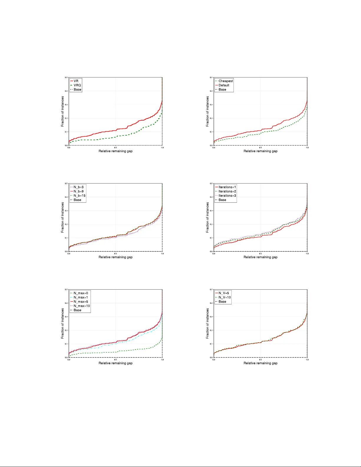
Axis-Aligned Relaxations for Mixed-In teger Nonlinear Programming Haisheng Zh u 1 , T aotao He 2 , and Mohit T a warmalani ∗ 1 1 Mitc h Daniels School of Business, Purdue Universit y , W est Lafa y ette, IN 47906 2 An tai School of Management, Shanghai Jiao-T ong Univ ersit y , Shanghai, China 200030 Marc h 20, 2026 Abstract W e presen t a no vel relaxation framew ork for general mixed-integer nonlinear programming (MINLP) grounded in computational geometry . Our approac h constructs polyhedral relaxations b y conv exifying ﬁnite sets of strategically chosen p oin ts, iterativ ely reﬁning the approximation to con verge to w ard the simultaneous con vex hull of factorable function graphs. The framework is underpinned by three key contributions: (i) a new class of explicit inequalities for pro ducts of functions that strictly improv e up on standard factorable and comp osite relaxation schemes; (ii) a pro of establishing that the simultaneous conv ex h ull of multilinear functions o ver axis- aligned regions is fully determined by their v alues at corner p oin ts, thereby generalizing existing results from hypercub es to arbitrary axis-aligned domains; and (iii) the in tegration of com- putational geometry tools, sp eciﬁcally vo xelization and Quic kHull, to eﬃcien tly approximate feasible regions and function graphs. W e implement this framew ork and ev aluate it on ran- domly generated p olynomial optimization problems and a suite of 619 instances from MINLPLib . Numerical results demonstrate signiﬁcant impro vemen ts ov er state-of-the-art b enc hmarks: on p olynomial instances, our relaxation closes an additional 20–25% of the optimalit y gap rela- tiv e to standard metho ds on half the instances. F urthermore, compared against an enhanced factorable programming baseline and Gurobi’s ro ot-node b ounds, our approach yields sup erior dual bounds on approximately 30% of MINLPLib instances, with roughly 10% of cases exhibiting a gap reduction exceeding 50%. Keywor ds— p olyhedral relaxation, vo xelization, mixed-integer nonlinear programming, computational geometry , conv ex extensions 1 In tro duction Algorithms to solve mixed-integer nonlinear programs (MINLPs) rely predominan tly on factor able pr o gr am- ming (FP), a framew ork that lev erages the recursiv e structure of nonlinear functions to construct conv ex relaxations [35, 49, 37, 34, 6]. FP represents nonlinear functions using their expression tree where lea v es represen t v ariables or constan ts and internal no des denote op erations (e.g., addition, multiplication). F or eac h in ternal no de, an auxiliary v ariable is in tro duced, and the relationship b et w een this v ariable and its op erands is relaxed using prop erties s peciﬁc to the op eration; notably , McCormic k env elop es are emplo yed to relax the m ultiplication no des. By systematically relaxing eac h op eration ov er the known b ounds of its argumen ts, FP transforms a nonconv ex problem into a tractable conv ex relaxation. ∗ corresp onding author: m taw arma@purdue.edu 1 F actorable programming (FP) remains the dominan t framew ork due to its scalability: the n um b er of auxiliary v ariables and constrain ts introduced is comparable to that of the original form ulation. How ever, this eﬃciency comes at the cost of tightness. FP relaxes each op eration indep enden tly ov er a hypercub e deﬁned b y v ariable bounds, thereby ignoring in terdependencies among v ariables induced b y linking constrain ts. This decoupling yields o verly conserv ativ e relaxations that admit feasible regions signiﬁcantly larger than the true feasible set, often including com binations of v ariable v alues that violate the original problem constrain ts. Alternativ e general-purp ose relaxation techniques include composite relaxations [21], reformulation- linearization technique (RL T) [44], and sum-of-squares (SOS) hierarchies [29]. While RL T and SOS re- laxations often require a proliferation of auxiliary v ariables, comp osite relaxations maintain a v ariable count similar to FP . Theoretically , comp osite relaxations are guaranteed to be tigh ter than FP and ha ve b een sho wn to be signiﬁcan tly tighter for p olynomial optimization problems [23]. F urthermore, there is an ex- tensiv e literature on conv exiﬁcation techniques for sp eciﬁc function structures. This includes results on m ultilinear functions [41, 2, 15], functions with indicator v ariables [19, 1], fractional functions [24], sup er- mo dular functions [52], quadratic forms [9, 16]. How ev er, such analyses hav e typically b een conﬁned to structured domains like hypercub es and simplices. While explicit conv ex en velopes for biv ariate functions o ver con vex p olygons exist and hav e shown promise [30, 31, 39], and FP has b een augmented with dis- cretization schemes [37, 40, 34], no systematic mechanism currently exists to construct conv ex relaxations that sim ultaneously a void excessive auxiliary v ariables and yields tight env elop es for factorable functions o ver general non-conv ex domains. This paper prop oses such a sc heme, implemen ts it for lo w-dimensional functions and regions, and demonstrates its eﬃcacy on a large collection of b enc hmark problems. Our framework builds on the expression tree represen tation central to FP , but in tro duces a fundamentally distinct relaxation strategy to address this limitation. The relaxations are constructed as the conv ex hull of ﬁnite sets of strategically chosen points iden tiﬁed via t wo appro ximation steps: (i) outer-appro ximation of the feasible set by an axis-aligned region, and (ii) piecewise-approximation of the inner functions asso ciated with eac h op erator. Although our approach also decomp oses functions in to low-dimensional atomic expressions, it leverages computational geometry to capture interdependencies among v ariables and functions, thereb y constructing pro v ably tighter relaxations than factorable programming. The cornerstone of our approach is a no vel relaxation technique for multilinear functions ov er axis-aligned regions. T o frame relaxation construction as such a problem, w e approximate feasible regions using vo xeliza- tion and graphs of functions using tessellations. V o xelization discretizes contin uous geometric domains in to a grid of v oxels indicating feasibility , while tessellation approximates the function graph with a union of p olygonal shap es. Standard FP can b e viewed as a sp ecial case that constructs relaxations ov er the coarsest v oxel, the b ounding h yp ercube. In contrast, general axis-aligned regions oﬀer opp ortunities for signiﬁcan tly tigh ter relaxations. Moreo ver, unlike FP , which loses the structure of inner functions b y replacing them with v ariables, our tessellation sc hemes preserve this structure while relaxing outer-functions. By adapting established computational geometry metho ds–suc h as discretizing lines [12], surfaces [45, 46], and p olyhe- dra [17]–to construct relaxations, our framework enables higher ﬁdelity conv ex relaxations without adding auxiliary v ariables, alb eit with extra computational eﬀort. Our tec hnique can also b e viewed as a generalization of McCormic k relaxation, whic h constructs the con vex h ull of four points on a bilinear product’s graph. This geometric interpretation has inspired tec hniques that focus on sp eciﬁc p oin ts whose conv ex extension yields v alid relaxations [14, 41, 48, 36]. Our construction represen ts each p oin t in an axis-aligned region as a con vex combination of sp eciﬁc corner points using a discrete Mark ov c hain. Using this represen tation, we pro ve that appropriately lifting these corner points in to a higher-dimensional space yields the ﬁnite collection of points required to con v exify multilinear compositions. Axis-aligned regions oﬀer greater ﬂexibility than hypercub es; reﬁning the vo xelization resolution al- lo ws for an arbitrarily close approximation of the feasible set. This approach extends b ey ond hierarchical con vexiﬁcation to explicitly exploit nonlinear and noncon vex structures. W e tak e adv antage of conv ergent v oxelization schemes with computational geometry to ols, such as the Quick Hull algorithm [3] to enhance relaxation quality . Notably , we prov e that our relaxation conv erges to the tigh test p ossible relaxation, the con vex hull of the function ov er the feasible domain, as the vo xelization resolution increases. W e ev aluate these relaxations on randomly generated p olynomial optimization problems [23] and 619 instances from MINLPLib [10]. F or polynomial optimization, our relaxation closes 20-25% of the gap on half of the instances, clearly dominating factorable programming, Gurobi ro ot-node [20], and comp osite relaxation [23]. F or MINLPLib , w e impro ve up on an enhanced FP baseline and Gurobi on appro ximately 2 30% of instances, closing 50% of the gap on 10% of them. Although constructing axis-aligned regions and con vexifying point sets incurs computational exp ense, the resulting relaxations are not signiﬁcantly harder to solv e than FP coun terparts, lik ely due to the absence of extra auxiliary v ariables and the sparsity of generated inequalities. Within MINLPLib , w e identiﬁed six c hallenging unsolv ed instances where our relaxation ac hieves a b ound sup erior to the ﬁnal b ounds rep orted b y solvers after many branch-and-bound iterations. T o illustrate, consider the following nonlinear program: max e x 1 − x 2 x 1 x 2 s.t. x 1 , x 2 ∈ [0 , 1] (1) Reform ulating with auxiliary v ariables t 1 , t 2 , t 3 : max t 1 t 2 s.t. t 1 = e t 3 t 3 = x 1 − x 2 t 2 = x 1 x 2 x 1 , x 2 ∈ [0 , 1] (2) FP relaxes the bilinear term t 1 t 2 o ver the v ariable b ounds (dashed rectangle in Figure 1(a)), which outer- appro ximates the feasible region. In contrast, our framework appro ximates the feasible domain by vo xeliza- tion (Figure 1(b)), pro ducing a signiﬁcantly tighter relaxation as depicted in Figure 1(c). 1 2 3 0 . 5 1 1 . 5 t 1 t 2 (a) 1 2 3 0 . 5 1 1 . 5 t 1 t 2 (b) (c) Figure 1: Comparison of relaxation ov er rectangular b ounds versus vo xelization T o our kno wledge, this pap er presen ts the ﬁrst general-purp ose application of v oxelization, tessella- tion, and QuickHull to systematically create MINLP relaxations. The framework reduces the relaxation of man y MINLPs to computational geometry tasks in low-dimensional spaces, guaranteeing conv ergence to the tigh test p ossible relaxation in structured settings. This application is enabled by: • T o ols to appro ximate arbitrary collections of functions using piecewise multilinear functions and vo x- elization supp orted with in terv al-arithmetic tec hniques [38], eliminating the need for extra auxiliary v ariables; • A foundational con vex extension prop ert y that p ermits simultaneous conv exiﬁcation of piecewise multi- linear functions ov er axis-aligned regions, iden tifying p oin t sets whose conv ex hull encompasses multiple function graphs sim ultaneously . The framework is supported by rigorous con vergence guarantees, demonstrating that the relaxation con verges to the conv ex hull of a collection of function graphs ov er arbitrary domains as the resolution increases. W e also develop sp ecialized techniques for products of univ ariate functions that pro v ably outp erform existing metho ds. Our to ols are implemented in a Julia -based framework built on JuMP [33], enabling eﬃcien t generation of relaxations that ac hieve sup erior p erformance on b enc hmark instances. Section 2 presents tw o-dimensional results. Section 2.1 provides new inequalities for the pro duct of tw o functions deﬁned ov er a rectangle, improving FP and comp osite relaxations [21]. This motiv ates p olyhedral 3 relaxations using computational geometry . Section 2.2 appro ximates the feasible domain via axis-aligned regions and prov es that the conv ex h ull of a bilinear term ov er such a region is ﬁnitely-generated. Section 2.3 com bines these approaches to construct p olyhedral relaxations for the pro ducts of univ ariate functions o ver arbitrary regions. Section 3 addresses m ultilinear comp ositions in n -dimensional space. Section 3.1 abstracts these problems by replacing function appro ximations with tessellations and constructing axis-aligned regions that incorp orate these tessellations. The core theoretical result then identiﬁes a ﬁnite set of p oin ts to con- v exify multilinear functions simultaneously ov er such regions. Section 3.2 prov es conv ergence to the conv ex h ull as the resolution of the approximation increases. Section 4 discusses our restricted implemen tation, describing t wo vo xelization metho ds (Sections 4.3, 4.4). Section 5 ev aluates performance on polynomial optimization problems (Section 5.1) and MINLPlib (Section 5.2), demonstrating improv ements ov er prev a- len t factorable programming relaxations. Finally , we explore h yp erparameters controlling approximation resolution to analyze the trade-oﬀ b et ween computational time and relaxation tigh tness. Notation: F or a set S , we denote its conv ex h ull as con v( S ) and its extreme points as v ert( S ). The corner points of an axis-aligned region H are denoted by corner( H ). The pro jection of a set S on to the subspace of v ariables x is written as pro j x ( S ). Finally , the cardinalit y of a ﬁnite p oin t set S is denoted as card( S ). The sequence 1 , . . . , m is denoted as [ m ]. 2 T o ols: Piecewise Appro ximation and Axis-Aligned Regions This section details the key to ols employ ed to construct relaxations, with particular emphasis on the relax- ation of function pro ducts, a critical step in relaxing factorable programs. Our approach pro ceeds in t w o stages: ﬁrst, appro ximating each nonlinear function via a piecewise linear function, and second, replacing the feasible domain with its v oxelization. These concepts are introduced in Sections 2.1 and 2.2, resp ectiv ely . T ogether, these steps deﬁne a ﬁnite set of p oin ts whose conv ex hull yields a relaxation of the pro duct ov er an arbitrary domain, as detailed in Section 2.3. W e demonstrate that this approac h can b e tuned to balance appro ximation ﬁdelit y and computational eﬃciency , establishing it as a foundational comp onen t for relaxing complex factorable expressions. 2.1 Multiplication of F unctions o ver a Rectangle In this subsection, we fo cus on relaxing the pro duct of tw o univ ariate functions ov er a rectangular domain. Sp eciﬁcally , we analyze the graph: G :=  ( x, µ ) ∈ [0 , 1] 2 × R   µ = f 1 ( x 1 ) f 2 ( x 2 )  , where eac h f i : [0 , 1] → R is an arbitrary nonlinear function. Although w e restrict the domain of x i to [0 , 1], our result generalizes to arbitrary interv als; since the functions are arbitrary , the general case can b e reduced to the [0 , 1] case via an aﬃne transformation. Our relaxation relies on pie c ewise-line ar appr oximation , demonstrating that approximating eac h f i generates a ﬁnite set of p oin ts whose conv ex hull provides a v alid relaxation for the graph G . This approach tigh tens the recen t comp osite relaxation introduced by He and T aw armalani [21]. Moreov er, b y tuning the approximation accuracy , w e can eﬀectively balance computational eﬃciency with the tigh tness of the resulting relaxation. T o contextualize our contribution, we ﬁrst review the comp osite relaxation framework prop osed by He and T aw armalani [21]. Their metho d improv es factorable programming relaxations by constructing a p olyhedral approximation U i for each individual function f i ( x i ), i = 1 , 2, within a lifted space. The product is then relaxed o ver the Cartesian pro duct U 1 × U 2 . Although the abilit y to choose the dimension of each U i oﬀers ﬂexibility to balance accuracy with com p utational cost as higher-dimensional approximations yield tigh ter relaxations, this approach suﬀers from tw o key limitations: 1. The pro jection of the relaxation fails to conv erge to the con vex hull of the graph of the product function as the dimension of the appro ximations increases. 2. The num b er of inequalities required to conv exify the pro duct ov er U 1 × U 2 gro ws exp onen tially with min  dim( U 1 ) , dim( U 2 )  , regardless of the actual n umber of inequalities required to describ e the con vex h ull of f 1 ( x 1 ) f 2 ( x 2 ). 4 In con trast, our tec hnique yields a tigh ter relaxation that conv erges to the con vex hull of the product’s graph, while eliminating redundant inequalities. W e ﬁrst illustrate this approach with an example, b efore pro viding a formal description of the metho d. Example 1. Consider the monomial x 2 1 x 2 2 over the domain [0 , 2] 2 . F or e ach i = 1 , 2 , we deﬁne two aﬃne under estimators: 2 x i − 1 and 4 x i − 4 . Using these, we c onstruct a c onvex under estimator for the monomial and c omp ar e its str ength against the c omp osite r elaxation pr op ose d by He and T awarmalani [21] and its limiting c ase in He and T awarmalani [22]. We ﬁrst pr esent our r elaxation. F or e ach i = 1 , 2 , we deﬁne the p olyhe dr al outer-appr oximation P i := n ( x i , t i )    max  0 , 2 x i − 1 , 4 x i − 4  ≤ t i ≤ 4 , x i ∈ [0 , 2] o . (3) By c omputing the c onvex envelop e of t 1 t 2 over P 1 × P 2 and substituting x 2 i ≤ t i ≤ 4 x i , we obtain the c onvex under estimator: r ( x ) := max { 0 , 4 x 2 1 + 4 x 2 2 − 16 , 8 x 1 + 8 x 2 − 20 } . The c omp osite r elaxation of [21] c annot utilize the se c ond under estimator 4 x i − 4 , as its upp er b ound c oincides with that of x 2 i over [0 , 2] . R estricting to only the under estimator 2 x i − 1 and its c orr esp onding upp er b ound 3 , The or em 1 of [21] yields the r elaxation: r 1 ( x ) := max ( 0 , 4 x 2 1 + 4 x 2 2 − 16 , 8 x 1 + 3 x 2 2 − 16 , 3 x 2 1 + 8 x 2 − 16 6 x 1 + 6 x 2 − 15 , 2 x 1 + 2 x 2 + 3 x 2 1 + 3 x 2 2 − 17 ) , as derive d in Example 2 of [21]. While the c omp osite r elaxation impr oves as the numb er of under estimators incr e ases, the limiting c ase–using inﬁnitely many under estimators for x 2 i –is given by Example 4 of [22]: r ∞ ( x ) := max  0 , Z x 2 2 1 − x 1 2  4 λ 2 − 4 + 4 x 1 − x 2 1 λ 2  4 λ 2 − 8 λ + 4 x 2 − x 2 2 (1 − λ ) 2  d λ  . A t x = (1 . 5 , 1 . 5) , wher e the true function value is 81 16 = 5 . 0625 , we c ompute: r 1 ( x ) = 6 x 1 + 6 x 2 − 15 = 3 , r ∞ ( x ) ≈ 3 . 274653 , and r ( x ) = 8 x 1 + 8 x 2 − 20 = 4 . Thus, r 1 ( x ) < r ∞ ( x ) < r ( x ) , demonstr ating that our r elaxation c onstructe d using just two under estimators p er variable c an b e tighter than the limiting c omp osite r elaxation b ase d on inﬁnitely many under estimators. In Example 1, the set P i emplo yed to outer-approximate x 2 i is a p en tagon. A step in constructing r ( · ) in volv ed computing the conv ex en velope of t 1 t 2 o ver P 1 × P 2 , follow ed b y pro jecting out the t i v ariables utilizing x 2 i ≤ t i ≤ 4 x i . Now, we deriv e an explicit con vex hull description for t 1 t 2 o ver an arbitrary p en tagon. Assume that the range of f i is [ f L i , f U i ], and supp ose that the graph of f i is outer-approximated b y a p en tagon deﬁned by the following vertices: v i 0 = (0 , f L i ) v i 1 = ( p i 1 , f L i ) v i 2 = ( p i 2 , b i ) v i 3 = (1 , f U i ) and v i 4 = (0 , f U i ) , (4) where 0 ≤ p i 1 < p i 2 ≤ 1, and f L i < b i < f U i . Theorem 1 characterizes the set: con v  ( x, t, t 1 t 2 )   ( x i , t i ) ∈ P i for i = 1 , 2  . Theorem 1. L et P i b e the p entagon deﬁne d by the vertic es in (4) for i = 1 , 2 and let P = P 1 × P 2 . Deﬁne the p ar ameters: r i 1 := p i 2 − p i 1 b i − f L i r i 2 := 1 − p i 2 f U i − b i and w i := 1 r i 1 − r i 2 . The c onvex envelop e of f 1 f 2 over P is given by max j =1 ,..., 6  α j , ( x, t )  + c j  , wher e α j denotes the j th r ow of the matrix:         0 0 f U 2 f U 1 0 0 f L 2 f L 1 ( f U 2 − f L 2 ) w 1 0 f L 2 − r 12 ( f U 2 − f L 2 ) w 1 b 1 0 ( f U 1 − f L 1 ) w 2 b 2 f L 1 − r 22 ( f U 1 − f L 1 ) w 2 ( f U 2 − b 2 ) w 1 ( f U 1 − b 1 ) w 2 b 2 − r 12 ( f U 2 − b 2 ) w 1 b 1 − r 22 ( f U 1 − b 1 ) w 2 ( b 2 − f L 2 ) w 1 ( b 1 − f L 1 ) w 2 b 2 − r 11 ( b 2 − f L 2 ) w 1 b 1 − r 21 ( b 1 − f L 1 ) w 2         5 and the c onstant term is c j = f U 1 f L 2 −  α j 1 + α j 2 p 21 + α j 3 f U 1 + α j 4 f L 2  . Similarly, the c onc ave envelop e of f 1 f 2 over P is given by min k =1 ,..., 6  β k , ( x, t )  + d k  , wher e β k denotes the k th r ow of the matrix:         0 0 f U 2 f L 1 0 0 f L 2 f U 1 ( f L 2 − f U 2 ) w 1 0 f L 2 − r 11 ( f L 2 − f U 2 ) w 1 b 1 0 ( f L 1 − f U 1 ) w 2 b 2 f L 1 − r 21 ( f L 1 − f U 1 ) w 2 ( f L 2 − b 2 ) w 1 ( b 1 − f U 1 ) w 2 b 2 − r 12 ( f L 2 − b 2 ) w 1 b 1 − r 21 ( b 1 − f U 1 ) w 2 ( b 2 − f U 2 ) w 1 ( f L 1 − b 1 ) w 2 b 2 − r 11 ( b 2 − f U 2 ) w 1 b 1 − r 22 ( f L 1 − b 1 ) w 2         , with the c onstant term d k = f U 1 f U 2 −  β k 1 + β k 2 + β k 3 f U 1 + β k 4 f U 2  . The con vex hull description comprises of 12 non-trivial linear inequalities. Notably , the comp osite relaxation also yields 12 inequalities when relaxing the pro duct f 1 ( x 1 ) f 2 ( x 2 ) using a single underestimator for eac h f i ( x i ) (see Theorems 1 and 2 in [21]). How ever, the inequalities deriv ed in Theorem 1 are strictly tighter and result in improv ed b ounds when included in the relaxation. Building on this insight, we subsequently demonstrate that the substan tial gains of comp osite relaxations o ver traditional factorable programming metho ds, as highligh ted in [23], can b e further enhanced using the techniques presented here. Theorem 1 is therefore of indep enden t in terest, pro viding inequalities that strictly dominate those in Theorems 1 and 2 of [21] and underpin the b eneﬁts that our relaxation pro vides relative to comp osite relaxation ov er rectangular domains. F urther b eneﬁts for non-rectangular domains are realized in Section 2.3. Instead of restricting the outer-appro ximation of the graph to a pentagon, we now consider a general p olytope P i . Even in this generalized setting, the resulting relaxation remains p olyhedral. Prop osition 2. F or i = 1 , 2 , let P i b e a p olytop e that outer-appr oximates the gr aph of f i ( · ) . Then, a p olyhe dr al r elaxation of G is given by the c onvex hul l of the set Q , deﬁne d as Q :=  ( x, t, µ )   µ = t 1 t 2 , ( x i , t i ) ∈ v ert( P i ) for i = 1 , 2  . Pr o of. Since P i is an outer-approximation of the graph of f i ( · ), it follo ws readily that a conv ex relaxation for G is giv en as follows: R := con v  ( x, t, µ )   µ = t 1 t 2 , ( x i , t i ) ∈ P i for i = 1 , 2  . By Theorem 8 of [48], w e conclude that R = conv( Q ). Prop osition 2 requires computing the con vex hull of ﬁnitely many p oin ts. Since these p oin ts reside in a ﬁve-dimensional space, we can leverage low-dimensional conv ex hull algorithms, such as QHull [3], to eﬃcien tly obtain the corresp onding hyperplane description. F urthermore, when the functions f i ( · ) do not app ear elsewhere in the formulation, the auxiliary v ariables t i can b e pro jected out. In this case, it suﬃces to compute the con vex hull in the ( x, µ ) space, namely , con v  ( x, µ )   µ = t 1 t 2 , ( x i , t i ) ∈ v ert( P i ) for i = 1 , 2  , whic h corresp onds to a three-dimensional conv ex hull computation and is therefore substantially more tractable than computing the conv ex hull of Q in a lifted space as in Theorem 1. Bey ond computational eﬃ- ciency , an additional adv antage of emplo ying computational geometry to ols is that they yield an irredundan t facet description. Consequently , the resulting relaxation constitutes a minimal form ulation, con taining no redundan t inequalities. F or instance, in the context of Example 1, Theorem 1 yields six inequalities, while QHull pro duces only three, resulting in a more compact relaxation. By leveraging computational geometry to ols, one can construct a sequence of p olyhedral relaxations through the progressive reﬁnement of the outer-approximations for each univ ariate function f i ( · ). Indeed, Theorem 8 formally establishes that this sequence con v erges to the conv ex hull of gr( f 1 f 2 ). W e illustrate this conv ergence by revisiting Example 1. Starting with the outer-approximation deﬁned in (3) and depicted in Figure 2(a), the resulting relaxation is shown in Figure 2(b). As additional gradient inequalities are incorp orated to appro ximate x 2 i , Figures 2(c)–(e) demonstrate that the relaxations b ecome progressiv ely tigh ter, with the ﬁnal relaxation closely approximating the conv ex hull. 6 x i f ( x i ) 0 1 2 0 1 2 3 4 (a) (b) (c) Num b er of gradien ts: 3 (d) Num b er of gradien ts: 5 (e) Num b er of gradien ts: 10 Figure 2: Approximation of x 2 1 x 2 2 via piecewise linear relaxations Finally , w e formally demonstrate that our relaxation yields a tighter relaxation than the comp osite relaxation (CR) in [21]. CR applies to a comp osite function ϕ ◦ f : [0 , 1] d → R deﬁned as ( ϕ ◦ f )( x ) = ϕ  f 1 ( x 1 ) , . . . , f d ( x d )  for x ∈ [0 , 1] d , where each inner-function f i ( · ) is univ ariate. CR assumes that, for each f i ( · ), there exists a vector of underestimating functions u i ( · ). It exploits ordering relations among the estimating functions u i ( · ) and their upp er b ounds a i b y em b edding them into a polytop e U i , and then conv exiﬁes the outer-function ϕ ( · ) o ver the product p olytop e U := Q d i =1 U i . Sp eciﬁcally , for eac h i ∈ [ d ], assume a pair ( u i ( x i ) , a i ) suc h that for all x i ∈ [0 , 1], a i 0 ≤ a i 1 ≤ · · · ≤ a in i , u ij ( x i ) ≤ min  f i ( x i ) , a ij  for j = 0 , . . . , n i . (5) That is, eac h u ij ( · ) underestimates f i ( · ) and is b ounded ab o v e by a ij . The comp osite relaxation introduces auxiliary v ariables u i and f i to represent u i ( x i ) and f i ( x i ) resp ectiv ely , and enco des the ordering constraints in to the p olytope U i deﬁned as follo ws: U i :=  ( u i , f i )   f L i ≤ f i ≤ f U i , u ij ≤ a ij , u ij ≤ f i for j ∈ { 0 , . . . , n i }  , where f L i (resp. f U i ) is a low er (resp. upp er) b ound of f i ( · ). Let U := Q d i =1 U i and deﬁne Φ U :=  ( f , u, µ )   µ = ϕ ( f ) , ( f , u ) ∈ U  . Given a pair  u ( x ) , a  , where u ( x ) =  u 1 ( x 1 ) , . . . , u d ( x d )  and a = ( a 1 , . . . , a d ), satisfying (5), the comp osite relaxation is deﬁned as C R  u ( x ) , a  :=  ( x, f , µ, u )   ( f , u, µ ) ∈ conv(Φ U ) , u ≥ u ( x )  . In contrast, our approac h av oids introducing v ariables for the estimating functions. Instead, it uses the underestimators u ij ( · ) to construct a p olyhedral outer-approximation of the graph of f i ( · ): P i :=  ( x i , f i )   f L i ≤ f i ≤ f U i , x i ∈ [0 , 1] , u ij ( x i ) ≤ f i for j ∈ { 0 , . . . , n i }  . (6) Let P := Q i ∈ [ d ] P i . Con vexiﬁcation of the outer-function ϕ ( · ) is then p erformed directly ov er P in the space of ( x, f ) v ariables, whereas the comp osite relaxation conv exiﬁes ϕ ( · ) ov er U in the higher-dimensional space of ( f , u ) v ariables. Next, w e show that our relaxation is tighter than the comp osite relaxation. 7 Prop osition 3. L et  u ( x ) , a  b e a p air satisfying (5). Deﬁne the set Φ P :=  ( x, f , µ )   µ = ϕ ( f ) , ( x i , f i ) ∈ P i for i ∈ [ d ]  , wher e P i deﬁne d as in (6). Then, con v  Φ P  ⊆ pro j ( x,f ,µ )  C R  u ( x ) , a  . Pr o of. It suﬃces to demonstrate that Φ P ⊆ pro j ( x,f ,µ )  C R  u ( x ) , a  , given that the latter set is con vex. Consider an arbitrary point ( x, f , µ ) ∈ Φ P and let u = u ( x ). By construction, ( f , u ) ∈ U and µ = ϕ ( f ), whic h implies ( f , u, µ ) ∈ Φ U ⊆ conv(Φ U ). Since u = u ( x ) also holds, the tuple ( x, f , µ, u ) b elongs to C R  u ( x ) , a  . Consequently , the pro jection ( x, f , µ ) lies within pro j ( x,f ,µ )  C R  u ( x ) , a  . 2.2 Multiplication of V ariables o ver an Arbitrary Domain In this subsection, we construct relaxations for the pro duct of tw o v ariables ov er an arbitrary b ounded domain D ⊂ R 2 . Sp eciﬁcally , we consider the graph: G :=  ( x, µ ) ∈ R 3   µ = x 1 x 2 , x ∈ D  . (7) A prev alent approach relies on the McCormick env elop e to relax the bilinear term o ver a rectangular b ounding b o x of D . How ev er, such relaxations are often weak when the geometry of D deviates signiﬁcantly from a rectangle. Our ob jective is to demonstrate how voxelization can b e leveraged to generate a sequence of p olyhedral relaxations that are tigh ter than standard McCormick relaxations and con verge to the con vex h ull of G . In computational geometry , v oxelization is the pro cess of con verting a geom etric ob ject into a set of discrete, grid-aligned v olumetric elemen ts known as voxels . Within our framew ork, the standard McCormick relaxation of G can b e interpreted as a trivial vo xelization of the domain D , wherein the en tire domain is appro ximated by a single global vo xel. W e make this observ ation explicit as follo ws: Remark 1. Given a b ounde d r e gion D ⊂ R 2 , we appr oximate it with a r e ctangular b ounding b ox [ x L 1 , x U 1 ] × [ x L 2 , x U 2 ] . We then c onstruct the c onvex hul l of the biline ar term over this voxel. This pr o c e dur e is e quivalent to c omputing the c onvex hul l of the biline ar term evaluate d at the four vertic es of the b ox: con v  ( x, x 1 x 2 )   x i ∈ { x L i , x U i } for i = 1 , 2  . Cle arly, the r esulting c onvex hul l is a valid p olyhe dr al r elaxation of G , if the voxel outer-appr oximates D . By systematically excising rectangles from the initial b ounding b o x, we obtain a reﬁned vo xelization. This approach yields tigh ter relaxations by computing the conv ex hull of the bilinear term o ver the resulting v oxelized domain. W e illustrate this pro cedure with the following example. Example 2. Consider a biline ar term x 1 x 2 deﬁne d over a nonc onvex domain D , given by: D :=  x ∈ R 2   x 2 ≤ 1 + log( x 1 ) , x 2 ≤ 1 − log( x 1 ) , x 1 ∈ [ e − 1 , e ] , x 2 ≥ 0  . In FP r elaxation, the domain D is appr oximate d by its b ounding b ox [ e − 1 , e ] × [0 , 1] , and the biline ar term is r elaxe d over this b ox. This single-voxel appr o ach is depicte d in the left p anel of Figur e 3. As shown, this r elaxation is signiﬁc antly lo oser than the c onvex hul l of the biline ar term over D . Observe that x 1 x 2 is shown as the r e d r e gion in Figur e 3. The r elaxation gap c an b e systematic al ly r e duc e d by r eﬁning the underlying voxelization. F or instanc e, by r emoving four r e ctangular r e gions fr om the initial b ounding b ox, and c omputing the c onvex hul l of the biline ar term over the r esulting r eﬁne d domain, we obtain a tighter r elaxation. This r eﬁnement is depicte d in the midd le p anel of Figur e 3. By c ontinuing this pr o c ess, the voxelize d r e gion incr e asingly c onforms to the ge ometry of D , and the r esulting r elaxation c onver ges towar d the true c onvex hul l, as il lustr ate d in the right p anel of Figur e 3. 8 1 2 3 0 . 5 1 1 . 5 x 1 x 2 1 2 3 0 . 5 1 1 . 5 x 1 x 2 1 2 3 0 . 5 1 1 . 5 x 1 x 2 Figure 3: Reﬁnement of the bilinear relaxation via v o xelization. The top row illustrates the domain D (teal) and its axis-aligned outer appro ximation (red boundary) with increasing lev els of accuracy . The b ottom row depicts the corresp onding three dimensional polyhedral relaxations (green). As the vo xelization is reﬁned from left to righ t, the polyhedral relaxation con v erges to ward the true con vex hull of the bilinear term o ver D . Al though these thr e e r elaxations vary in tightness, they shar e a crucial structur al pr op erty: they ar e al l p olyhe dr al. Sp e ciﬁc al ly, the c onvex hul l in e ach c ase is gener ate d by a ﬁnite set of p oints. As we wil l establish later, these gener ators c orr esp ond pr e cisely to the c orner p oints of the voxelize d r e gions, which ar e highlighte d in blue in Figur e 3. T o formalize the construction presented in Example 2, w e introduce several deﬁnitions. First, to ensure that the resulting relaxations remain p olyhedral, w e require vo xelizations to b e axis-aligned: this prop ert y is shared b y the three vo xelizations illustrated in the preceding example. Deﬁnition 1. A planar r e gion H is axis-aligne d if it c an b e expr esse d as a ﬁnite union of r e ctangles, e ach with sides p ar al lel to the c o or dinate axes. Throughout this pap er, we denote by B ( H ) the set of constituen t rectangles deﬁning H , and by disc( H ) the set of vertices asso ciated with the rectangles in B ( H ). W e remark that for a given axis-aligned region, disc( H ) is not unique. Ho wev er, we do not concern ourselves with this issue since an y such represen tation will suﬃce for our purp ose. W e now formally deﬁne the sp eciﬁc subset of p oin ts that serve as generators for the conv ex hulls illustrated in Example 3. Although disc( H ) encompasses all vertices of the underlying rectangles, the relaxation is ultimately determined by a sp eciﬁc subset of these p oin ts, which w e refer to as c orner p oints . Deﬁnition 2. A p oint ( v 1 , v 2 ) is a c orner p oint of a planar axis-aligne d r e gion H if v i is an extr eme p oint of con v { ( x 1 , x 2 ) | x ∈ H , x i ′ = v i ′ , i ′ ∈ { 1 , 2 } \ { i }} . The set of al l c orner p oints of H is denote d by corner( H ) . It is imp ortan t to note that every corner-p oin t of H must b elong to the set of discretization p oin ts disc( H ). Indeed, if a p oin t is not a v ertex of any constituen t rectangles, it lies in the relativ e in terior of some face F of a rectangle. Since F has dimension at least one, there exists a line segmen t parallel to the one of tw o co ordinate axes that lies within F and contains the p oin t in its relative in terior. F urthermore, our deﬁnition of corner p oin ts diﬀers from that of extreme p oin ts of p olytop es, b y restricting the allo wable directions of such line segmen ts. F or instance, applied to the p olytope  x ∈ R 2 + | x 1 + x 2 ≤ 1  , our deﬁnition w ould identify all p oin ts on the line segment joining (1 , 0) to (0 , 1) as corner p oin ts. W e now present how the bilinear graph G can b e relaxed o ver any b ounded domain D . 9 Prop osition 4. L et H ⊂ R 2 b e an axis-aligne d outer-appr oximation of the domain D , and deﬁne R := con v  ( x, x 1 x 2 )   x ∈ H  . Then, R is a p olyhe dr al r elaxation of G that c oincides with the c onvex hul l of Q , wher e Q :=  ( x, µ )   µ = x 1 x 2 , x ∈ corner( H )  . Before proceeding to the pro of, we discuss its primary tec hnical challenge. Given an arbitrary p oin t v = ( v 1 , v 2 ) in an axis-aligned region H , we m ust demonstrate that ( v , v 1 v 2 ) can be expressed as a conv ex com- bination of points in Q . A natural approach is an iter ative c o or dinate-wise c onvex de c omp osition . Sp eciﬁcally , b y ﬁxing the second co ordinate, one can express ( v 1 , v 2 , v 1 v 2 ) as a conv ex com bination of ( v L 1 , v 2 , v L 1 v 2 ) and ( v U 1 , v 2 , v U 1 v 2 ), where v L 1 and v U 1 denote the endp oin ts of the line segment forming the slice { x | ( x, v 2 ) ∈ H} . By iteratively alternating the ﬁxed co ordinate, one might exp ect to even tually reach the corner p oin ts of H . Ho wev er, as illustrated in Figure 4, this greedy co ordinate-wise approach may enter a cycle. In the example sho wn, resolving the point v = (2 , 1) through successive co ordinate-wise decomp ositions can return to the starting p oin t after a ﬁnite sequence of steps, failing to terminate at the corner p oin ts. Consequently , our pro of must employ a more global argument to establish the representation. − 1 1 2 3 4 5 6 2 4 6 v x 1 x 2 Figure 4: Illustration of a cycle (indicated in blue) in the iterativ e co ordinate-wise decomp osition. Starting from p oin t v , alternating decomp ositions along the x 1 and x 2 axes return to v after four iterations, demonstrating that the greedy pro cedure ma y fail to yield a ﬁnite representation via corner p oin ts. T o circumv ent the cyclic b eha vior illustrated in Figure 4, we abandon the greedy deterministic iterative decomp osition in fav or of one that expresses the initial p oin t v as the exp ectation of the corner p oin ts under a probability distribution. Sp eciﬁcally , our pro of constructs a Marko v chain to trac k the evolution of the decomp osition pro cess. Within this framework, the probability distribution at each time step is interpreted as a con vex decomp osition of v . By analyzing the limiting b eha vior of the Marko v chain, we establish that the limiting distribution yields a v alid representation of v as a con vex combination of corner p oin ts in H . F or completeness, we brieﬂy review key concepts of Marko v chain theory , see [18, Chapter 11] for further details. A Marko v c hain is deﬁned b y a ﬁnite state sp ac e X and a tr ansition matrix T . A sequence of random v ariables ( X 1 , X 2 , X 3 , . . . ) constitutes a Marko v chain with state space X and transition matrix T if the Markov pr op erty holds. Sp eciﬁcally , for all x, y , all t ≥ 2, and an y history even t H t − 1 = ∩ t − 1 s =1 { X s = x s } suc h that Pr( H t − 1 ∩ { X t = x } ) > 0, w e hav e Pr  X t +1 = y   H t − 1 ∩ { X t = x }  = Pr { X t +1 = y | X t = x } = T ( x, y ) . A state x is termed absorbing if the chain cannot leav e it; that is, T ( x, x ) = 1. A Mark ov chain is absorbing if it p ossesses at least one absorbing state and if every state can reach an absorbing state potentially ov er m ultiple steps. In such a chain, a non-absorbing state is called tr ansient . Let T t denote the t -step transition matrix, where the entry T t ( x, y ) represen ts the probability of b eing in state y after t steps, given an initial state x . The transition matrix of an absorbing Marko v ch ain is written in canonical form as: T =  Q R 0 I  , 10 where Q describ es transitions among transient states, R describ es transitions from transient to absorbing states, and I is the identit y matrix corresp onding to the absorbing states. The long-term b eha vior of an absorbing Mark ov chain is characterized by the limiting transition matrix T ∗ : T ∗ := lim t →∞ T t =  0 ( I − Q ) − 1 R 0 I  , (8) where the matrix N = ( I − Q ) − 1 is kno wn as the fundamental matrix . The entries of the pro duct B = N R giv e the probabilities of absorption in to eac h speciﬁc absorbing state, conditioned on starting from a transien t state. T o leverage Marko v c hain theory , we must formally sp ecify a state space and a transition matrix within our geometric context. T o this end, we prop ose the iterative pro cedure detailed in Algorithm 1. Given an axis-aligned region H , we deﬁne the initial state space X as the union of the corner p oin ts of the constituent rectangles of H , denoted by disc( H ). F or each point v in X , we in vok e the pro cedure end ( v, H ) to decomp ose v in to a pair of endp oin ts ( v l , v r ) along one of the co ordinate axes. Sp eciﬁcally , let i b e the smallest index in { 1 , 2 } and let j = { 1 , 2 } \ { i } b e suc h that v i is not an extremum of the slice { x i | x ∈ H , x j = v j } . W e deﬁne the endp oin ts v l and v r as the extrema of this slice: v l = arg min { x i | x ∈ H , x j = v j } and v r = arg max { x i | x ∈ H , x j = v j } . In this case, v l and v r are added to the state space X (if not already present), and the transition probabilities from v are determined by the conv ex multipliers speciﬁed in line 13 of Algorithm 1. If no such index i exists, w e set v l = v r = v and assign a transition probability of one from v to itself. W e note that a p oin t is a corner p oin t if and only if it is co ordinate-wise extremal; that is, for a corner p oin t ( v 1 , v 2 ), v 1 is an extreme p oin t of { x | ( x, v 2 ) ∈ H } and v 2 is an extreme p oin t of { y | ( v 1 , y ) ∈ H} . Consequently , when v l = v r = v , w e identify v as a corner-p oin t of H . Algorithm 1 A Marko v chain represen tation for co ordinate-wise con vex decomp ositions ov er pla- nar axis-aligned regions Input: An axis-aligned region H Output: A Mark ov chain with state space X and transition matrix T 1: Initialize state space X ← disc( H ) 2: Initialize unpro cessed stack U ← X 3: while U is not empty do 4: v ← p op( U ) 5: ( v l , v r ) ← end ( v , H ) 6: if v l  = v r then 7: for u ∈ { v l , v r } do 8: if u / ∈ X ∪ U then 9: X ← X ∪ { u } 10: Push u onto the stack U 11: end if 12: end for 13: Find λ ∈ [0 , 1] such that v = λv l + (1 − λ ) v r 14: Set T ( v , v l ) ← λ and T ( v , v r ) ← 1 − λ 15: else 16: Set T ( v , v ) ← 1 17: end if 18: end while In the follo wing lemma, we pro ve that Algorithm 1 terminates after ﬁnitely many iterations, yielding a ﬁnite Mark ov c hain. Subsequently , we analyze its limiting b eha vior. The core of the pro of, detailed 11 − 1 1 2 3 4 − 1 1 2 3 4 x y (a) Axis-aligned region H X 0 1 2 3 4 Y 0 1 2 3 4 s 1 s 2 s 3 s 4 s 5 s 6 s 7 s 8 s 9 s 10 1 1 1 1 1 1 0 . 33 0 . 66 0 . 33 0 . 66 0 . 5 0 . 5 0 . 5 0 . 5 (b) Corresp onding Marko v chain Figure 5: Illustration of the conv ex extension Marko v chain: (a) The axis-aligned region H and (b) the resulting sto c hastic transitions. in App endix A.2, relies on the observ ation that corner p oin ts of H constitute absorbing states within the Mark ov c hain. Consequently , the existence of a limiting transition matrix T ∗ ensures that every state can ultimately b e expressed as a conv ex combination of these corner-p oin ts. Notably , we establish this result for a general bilinear function ov er H , thereby enabling its application to the more general setting discussed in Section 2.3, where w e consider the pro duct of t wo functions ov er an arbitrary domain. Lemma 1. Given an axis-aligne d r e gion H ⊆ R 2 , Algorithm 1 terminates in ﬁnitely many iter ations, yielding an absorbing Markov chain ( X , T ) for which the c orner p oints of H serve as the absorbing states. Mor e over, for any biline ar function ℓ : H → R , we have that for every x ∈ X  x, ℓ ( x )  = X v ∈ corner( H ) T ∗ ( x, v ) ·  v , ℓ ( v )  , wher e T ∗ denotes the limiting tr ansition matrix deﬁne d as in (8) . With this lemma, w e pro ceed to the pro of of Prop osition 4. Pr o of of Pr op osition 4. First, observe that R is a con vex relaxation of G , since D ⊆ H . W e now demonstrate that R = conv( Q ), thereb y establishing the p olyhedralit y of the relaxation. The inclusion conv( Q ) ⊆ R follo ws directly from the facts that Q ⊆ R and R is a conv ex set. T o prov e the reverse inclusion, it suﬃces to show that any p oin t ( x, x 1 x 2 ) with x ∈ H can b e expressed as a conv ex combination of p oin ts in Q . Let H b e a rectangle in B ( H ) con taining x . By the conv ex extension property of bilinear term o ver axis-aligned rectangles [41, 48], w e hav e ( x, x 1 x 2 ) = X v ∈ v ert( H ) λ v ( v , v 1 v 2 ) , where { λ v } are con vex multipliers. Since vert( H ) ⊆ disc( H ) ⊆ X , w e may inv oke Lemma 1 to write ( x, x 1 x 2 ) = X v ∈ v ert( H ) λ v X w ∈ corner( H ) T ∗ ( v , w )( w, w 1 w 2 ) . Th us, ( x, x 1 x 2 ) is a con vex combination of p oin ts in Q . 12 0 0 . 5 1 1 . 5 2 2 . 5 3 0 0 . 5 1 1 . 5 x 1 x 2 0 0 . 5 1 1 . 5 2 2 . 5 3 0 0 . 5 1 1 . 5 x 1 x 2 0 0 . 5 1 1 . 5 2 2 . 5 3 0 0 . 5 1 1 . 5 x 1 x 2 Figure 6: Multiplication of functions ov er a nonconv ex domain 2.3 Multiplication of F unctions o ver an Arbitrary Domain In this subsection, w e address b oth c hallenges discussed in Sections 2.1 and 2.2 simultenaeously . Sp eciﬁcally , w e consider the graph of the pro duct of t wo univ ariate functions: G :=  ( x, µ ) ∈ R 3   µ = f 1 ( x 1 ) f 2 ( x 2 ) , x ∈ D  , where each f i : [ x L i , x U i ] → R is an arbitrary nonlinear function and D is a subset of [ x L , x U ]. T o obtain a p olyhedral relaxation for G , the prev alent FP approach introduces auxiliary v ariables t i to represen t each univ ariate function f i ( x i ), subsequen tly relaxing the graph of f i ( · ) and the bilinear term t 1 t 2 o ver the domain D indep enden tly . In contrast, our approach simultaneously handles the nonlinearities and the nonconv exity of the domain. By integrating the outer-approximation of the univ ariate functions with the vo xelization of the domain, w e construct a sequence of p olyhedral relaxations that con verges to the conv ex hull of G . Example 3. Combining the two pr e c e ding examples, c onsider x 2 1 x 2 2 over the fol lowing domain: x 2 ≤ 1 + log( x 1 ) x 2 ≤ 1 − log( x 1 ) x 1 ∈ [ e − 1 , e ] , x 2 ≥ 0 . We c onstruct a pie c ewise line ar under estimator u i ( · ) for x 2 i using its gr adients, while employing line ar inter- p olation as the over estimator o i ( · ) . The br e akp oints of pie c ewise line ar functions divide [ e − 1 , e ] × [0 , 1] into r e ctangular b oxes. After r emoving b oxes outside the domain, we obtain an axis-aligne d outer-appr oximation for the domain. Over this axis-aligne d r e gion, we c onvexify t 1 t 2 with u i ( x i ) ≤ t i ≤ o i ( x i ) for i = 1 , 2 . Figur e 6 demonstr ates that the r elaxation is p olyhe dr al and c onver ges to the c onvex hul l of the gr aph. This c onver genc e is achieve d by simultane ously r eﬁning the pie c ewise-line ar estimators of x 2 i and the voxelization of the domain. W e now formalize this construction. Let u i ( · ) and o i ( · ) denote piecewise aﬃne functions that underes- timate and ov erestimate the univ ariate function f i ( · ) ov er the interv al [ x L i , x U i ], resp ectiv ely . 1 Let H b e an 1 While the individual aﬃne segments provide lo cal b ounds, we allow them to b e discontin uous at breakp oin ts. Since w e typically restrict x i to a region where u i ( x i ) and o i ( x i ) are b oth aﬃne in the interior, with a slight abuse of notation, ev en at the end-points of such interv als, we ev aluate u i ( x i ) and o i ( x i ) using the same estimator. When m ultiple rectangles containing x are in the consideration set, we will assume that the smallest underestimator and the largest ov erestimator ov er the rectangles containing x are used to ev aluate u i ( x i ) and o i ( x i ) resp ectiv ely . 13 axis-aligned outer-appro ximation of the domain D . Then, we obtain the following conv ex relaxation: R := con v  ( x, t 1 t 2 )   x ∈ H , u i ( x i ) ≤ t i ≤ o i ( x i ) for i = 1 , 2  . (9) As in our previous constructions, we aim to represent the relaxation R as the conv ex hull of a ﬁnite set of p oin ts. T o ac hieve this, we integrate the breakp oints of piecewise-linear estimators with the corner-p oin ts of the axis-aligned region H . The breakp oin ts of the estimators divide [ x L , x U ] into rectangular cells that form its cov er 2 . Sp eciﬁcally , let D b e a rectangular cov er of [ x L , x U ] such that for ev ery rectangle H ∈ D , the four piecewise linear functions u i ( · ) and o i ( · ) ( i = 1 , 2) are aﬃne ov er H . Using this cov er D , we lift a ﬁnite set of p oin ts in H to deﬁne: Q := [ H ∈D n ( x, t 1 t 2 )    x ∈ corner( H ∩ H ) , t i ∈  u i ( x i ) , o i ( x i )  for i = 1 , 2 o . Giv en a set S ⊆ [ x L , x U ] and the cov er D of [ x L , x U ], we construct a cov er of S by intersecting eac h element of D with S . This yields a v alid co ver b ecause S = S ∩ [ x L , x U ] = S ∩ S H ∈D H = S H ∈D S ∩ H , where the ﬁrst equality holds by the deﬁnition of S , second b ecause D is a cov er of [ x L , x U ], and the third by the distributiv e law. This motiv ates our next deﬁnition. Deﬁnition 3 (grid cov er) . L et G b e a grid in R n and let O ⊆ R n . The grid c over of O induc e d by G is P = { v ∩ O : v is a c el l of G, v ∩ O  = ∅ } . As an example, consider the shaded axis-aligned region depicted in Figure 7 obtained by removing tw o dotted rectangles from [ x L , x U ]. The grid, drawn in dashed lines, induces a grid cov er of the shaded region sho wn as cells separated by thick red lines. Observe that the pro jection of Q on x -space is a grid cov er Figure 7: Removing rectangles from a grid of H . W e pro ve next that conv( Q ) yields R . The pro of exploits that any set S and its cov er S 1 , . . . , S m suc h that S i ⊆ S satisfy con v( S ) = conv  ∪ m j =1 con v ( S j )  . This is used to sho w that an y p oin t in the set  ( x, t 1 t 2 )   x ∈ H ∩ H , u i ( x i ) ≤ t i ≤ o i ( x i ) for i = 1 , 2  b elongs to conv ex hull of the union deﬁning Q . Theorem 5. L et u i ( · ) and o i ( · ) denote pie c ewise line ar under- and over-estimators of f i ( · ) on [ x L , x U ] , r esp e ctively, and let H b e an axis-aligne d outer appr oximation of D . Then, R c onstitutes a c onvex r elaxation of G and c oincides with the c onvex hul l of Q . Pr o of. Since eac h p oin t in G is contained in R and R is conv ex, it follows that conv( G ) ⊆ R . W e now show that R = conv( Q ). Since { H ∩ H} H ∈D forms a grid cov er of H induced by D , it follows that R can b e expressed as the con vex hull of ∪ H ∈D R H , where R H := con v  ( x, t 1 t 2 )   x ∈ H ∩ H , u i ( x i ) ≤ t i ≤ o i ( x i ) for i = 1 , 2  . The pro of is complete if we show that for every H ∈ D , R H = con v ( Q H ), where Q H := n ( x, t 1 t 2 )    x ∈ corner( H ∩ H ) , t i ∈  u i ( x i ) , o i ( x i )  for i = 1 , 2 o . 2 A collection of subsets of a set S that include each p oin t of S in at least one element 14 Clearly , conv( Q H ) ⊆ R H since Q H ⊆ R H and R H is conv ex. T o establish the reverse inclusion, w e consider a p oin t ( ¯ x, ¯ µ ) ∈ R H with ¯ µ = ¯ t 1 ¯ t 2 , where, for i ∈ { 1 , 2 } , ¯ t i ∈ [ u i ( ¯ x i ) , o i ( ¯ x i )]. F or i = 1 , 2, let λ i b e such that ¯ t i = λ i o i ( ¯ x i ) + (1 − λ i ) u i ( ¯ x i ). Deﬁne ℓ ( x ) = Q i =1 , 2 λ i o i ( x i ) + (1 − λ i ) u i ( x i ), and observ e that ℓ ( x ) is a bilinear expression in x and ℓ ( ¯ x ) = ¯ µ . Since H ∩ H is axis-aligned and ℓ ( x ) is bilinear ov er H , it follows b y Lemma 1 that there exists a subset V of corner( H ∩ H ) such that ( ¯ x, ¯ µ ) = P v ∈ V T ∗ ( x, v ) · ( v , ℓ ( v )). Since w e hav e expressed ( ¯ x, ¯ µ ) as a con vex combination of p oin ts in Q H , it follo ws that R H ⊆ con v ( Q H ). As the under- and ov er-estimators u i and o i con verge to f i o ver [ x L i , x U i ] for i = 1 , 2, and the outer appro ximation H conv erges to the domain D , con v ( Q H ) conv erges to con v ( G ). W e will prov e this result in Theorem 8. 3 Multilinear comp ositions with Linking Constrain ts In this section, we generalize our constructions to multilinear comp ositions M ◦ f o ver a domain D deﬁned b y linking constraints. Sp eciﬁcally , we consider a multilinear outer-function M : ( t 1 , . . . , t k ) ∈ R m 1 × · · · × R m k 7→ R , where k ≥ 2 and m k ≥ 1 for each i ∈ [ k ]. The inner-function is deﬁned as f ( x ) =  f 1 ( x 1 ) , . . . , f k ( x k )  , where for i ∈ [ k ], f i : x i ∈ X i ⊆ R n i 7→ R m i is a nonlinear function. In addition, w e assume that the domain is deﬁned b y general linking constraints, that is, D :=  x   x i ∈ X i for i ∈ [ k ] , g ( x ) ≤ 0  , where g ( · ) is a vector of nonlinear functions. W e are interested in constructing p olyhedral relaxations for the graph of multiline ar c omp osition (M ◦ f ) = M  f 1 ( x 1 ) , . . . , f k ( x k )  , that is, gr(M ◦ f ) :=  ( x, µ )   µ = (M ◦ f )( x ) , x ∈ D  . In Section 3.1, we extend the notion of axis-aligned region from simple planar sets to the more general domain D deﬁned ab o ve. Given an axis-aligned outer-approximation H of D , we obtain a p olyhedral relaxation of gr(M ◦ f ) by taking the conv ex hull of a ﬁnite set of p oin ts generated from the corner p oin ts of H . T o ac hieve this, the primary technical c hallenge is to generalize the Marko v c hain based decomp osition algorithm prop osed in Lemma 1. Then, w e further generalize our results to a vector of multilinear comp ositions. Finally , in Section 3.2, w e present tw o conv ergence results for t wo sp ecial cases of this framew ork. 3.1 Axis-aligned approximations and multilinear comp ositions As in the previous section, we ﬁrst identify a region P i that serves as an outer-approximation of the graph of eac h inner function f i ( x i ). Subsequen tly , we replace the functions with auxiliary v ariables t i and relax the multilinear composition of a multiv ariate function deﬁned o ver the Cartesian pro duct of these outer appro ximations: M( t 1 , t 2 , · · · , t k ) ( x i , t i ) ∈ P i , i ∈ [ k ] Giv en that computing an outer appro ximation of the graph of a general multiv ariate function is computa- tionally challenging, our implementation fo cuses on functions that are pro ducts of univ ariate comp onen ts although our constructions apply more generally . T o address the linking constraints, we introduce the concept of p olytopal tessellation, which provides a discretization of the feasible region. Deﬁnition 4 (Polytopal T essellation) . A p olytopal tessellation of a r e gion is a c over of that r e gion with a ﬁnite numb er of p olytop es that do not overlap in the interior. The c onstituent p olytop es ar e r eferr e d to as the c el ls of the tessel lation. 15 T o illustrate how tessellation facilitates the handling of linking constraints, consider the following exam- ple: M(2 x 1 + x 2 , y ) := (2 x 1 + x 2 ) y s.t. x 1 + x 2 ≤ 1 , y ≤ 1 x 1 , x 2 , y ≥ 0 The function M(2 x 1 + x 2 , y ) is a m ultilinear comp osition of linear functions, the domain of ( x 1 , x 2 ) is a simplex S and that of y ∈ [0 , 1]. Let S admit a tessellation S = S 1 ∪ S 2 ∪ S 3 , where S 1 = { ( x 1 , x 2 ) | x 1 + x 2 ≤ 1 , x 1 ≥ 0 , x 2 ≥ 0 . 5 } S 2 = { ( x 1 , x 2 ) | x 2 ≥ x 1 , x 1 ≥ 0 , x 2 ≤ 0 . 5 } S 3 = { ( x 1 , x 2 ) | x 1 + x 2 ≤ 1 , x 1 ≥ x 2 , x 2 ≥ 0 } Similarly , [0 , 1] admits a tessellation [0 , 1] = [0 , 1 3 ] ∪ [ 1 3 , 2 3 ] ∪ [ 2 3 , 1]. The pro duct of the tessellations is depicted in Figure 8. Now, supp ose that the problem contains the following constrain t linking x 2 and y : 2 x 2 − 3 y ≤ 0 Observ e that the cell S 1 × [0 , 1 3 ] of the pro duct tessellation is entirely excluded by this constraint. Conse- quen tly , S × [0 , 1] \ S 1 × [0 , 1 3 ] constitutes a relaxation of the feasible domain (see Figure 8). Sp eciﬁcally , S × [0 , 1] \ S 1 ×  0 , 1 3  can b e viewed as a set that generalizes axis-aligned regions deﬁned in Section 2.2. By applying a con vex extension argument similar to the one used in Section 2.2, it suﬃces to consider only a ﬁnite set of identiﬁable p oin ts to conv exify M ov er this relaxation. T o formally show this result, we expand the deﬁnition of axis-aligned regions and their corner p oin ts to include more general structures. Deﬁnition 5. A subset H in R n 1 × · · · × R n k is axis-aligned if it c an b e expr esse d as a ﬁnite union of pr o ducts of p olytop es as fol lows: n [ i =1 k Y j =1 P ij , wher e for e ach j ∈ [ k ] , the sets P 1 j , . . . , P nj b elong to the same Euclide an sp ac e R n j . W e deﬁne a corner p oin t of such an axis-aligned region as follows: Deﬁnition 6. L et H b e an axis-aligne d r e gion in R n 1 × · · · × R n k . A p oint ( v 1 , v 2 , . . . , v k ) ∈ R n 1 × R n 2 × · · · × R n k is a corner p oin t of H if, for e ach j ′ ∈ [ k ] , the ve ctor v j ′ is an extr eme p oint of the slic e con v  ( x 1 , . . . , x k ) ∈ H   x j = v j for al l j ∈ [ k ] \ { j ′ }  . The set of c orner p oints of H wil l b e denote d as corner( H ) . W e will refer to S n i =1 Q k j =1 v ert( P ij ) as disc( H ). Once again, corner( H ) ⊆ disc( H ) b ecause if a point v ∈ H \ disc( H ), then there exists an i such that v ∈ Q k j =1 P ij and a j such that v j ∈ vert( P ij ). Since the slice of H , with x j ′ = v j ′ for all j ′ ∈ [ k ] \{ j } must include P ij , v cannot b e an extreme p oin t of the con vex h ull of this slice. W e now demonstrate that, to conv exify a multilinear function o ver an axis-aligned region, it suﬃces to ev aluate the function solely at its corner p oin ts. W e ﬁrst mention that, to conv exify a m ultilinear function o ver a pro duct of p olytop es Q k i =1 P i , it suﬃces to consider only the corner p oin ts. This result follows from Theorem 1.2 in [41]. Lemma 2 (Rikun [41]) . L et M b e a multiline ar function over a pr o duct of p olytop es Q k i =1 P i , wher e P i ⊂ R n i . Then the c onvex hul l of the gr aph of M is the c onvex hul l of the set ( ( v , µ )      µ = M( v ) , v ∈ k Y i =1 v ert( P i ) ) wher e vert( P i ) denotes the set of vertic es of P i . 16 2 x 2 − 3 y = 0 Figure 8: Pro duct of tesselations Due to Lemma 2, ev aluating a multilinear function o ver product of p olytopes requires solely the vertices. W e no w demonstrate that, b y emplo ying con vex extension argumen ts, this set can b e further reduced to the corners of the axis-aligned region itself. T o this end, Algorithm 2 constructs a general con vex extension Mark ov chain for H = S n i =1 Q k j =1 P ij . The ﬁniteness of the resulting Marko v c hain is sho wn in Theorem 6 using the ﬁniteness of card(vert( P ij )) for all ( i, j ). This construction generalizes the conv ex extension Mark ov chain in tro duced in Section 2.2. W e now demonstrate that, for each vertex of the pro duct-of-polytop es structure deﬁning the axis-aligned region H , the chain’s limiting distribution expresses the vertex as a con vex com bination of the corners of H . The pro of of Theorem 6 closely parallels the results in Section 2.2, although it addresses sev eral additional technicalities that arise due to the abstraction of function approx imation and the higher-dimensional setting. Theorem 6. Given an axis-aligne d r e gion H , A lgorithm 2 terminates in ﬁnitely many iter ations, yielding an absorbing Markov chain ( X , T ) for which the c orner p oints corner( H ) serve as the absorbing states. Mor e over, for any multiline ar function M : H → R , we have that for every x ∈ X :  x, M( x )  = X v ∈ corner( H ) T ∗ ( x, v ) ·  v , M( v )  . (10) Consider x ∈ P i = Q k j =1 P ij ⊆ H such that x j = P v ′ j ∈ vert( P ij ) λ ( v ′ j ) · v ′ j is a r epr esentation of x j as a c onvex c ombination of vertic es in P j . Then,  x, M( x )  = X v ′ ∈ vert( P i ) X v ∈ corner( H )   k Y j =1 λ ( v ′ j )   T ∗ ( v ′ , v ) ·  v , M( v )  . (11) Pr o of. Since H is a ﬁnite union of pro ducts of p olytopes, w e construct v ectors consisting of extreme p oin ts for eac h co ordinate space R n j ( j ∈ [ k ]). The j th v ector is deﬁned as the lexicographically sorted list of extreme p oin ts in S n i =1 v ert( P ij ), where n is the num b er of pro ducts of p olytopes in H . W e will show that the state space X of the Mark ov chain is a subset of the grid formed b y the Cartesian product of these v ectors. Since the n umber of p olytop es is ﬁnite, this grid–and thus X –is ﬁnite. Consequently Algorithm 2 terminates ﬁnitely , since Step 12 only pushes a p oin t v ′ to the stac k if it is not already in X ∪ U . It remains to show that ev ery p oin t generated at Step 10 lies on this grid. W e pro ve by induction that if the stack U contains only grid points, then any p oin t added at Step 16 is also a grid p oin t. The base case holds b ecause the initial vertices of the constituent p olytopes are grid points b y construction. Assume that the p oin t v p opped from U at Step 4 is a grid p oin t. Then, the vectors v i generated at Step 10 are extreme p oin ts of the following slice obtained by ﬁxing all co ordinates except those in R n j : S j = con v    x j       x ∈ n [ i =1 k Y j =1 P ij , x j ′ = v j ′ ∀ j  = j ′    . 17 Algorithm 2 A Mark ov chain represen tation for co ordinate-wise conv ex decomp ositions ov er gen- eral axis-aligned regions Input: An axis-aligned region H = S n i =1 Q k j =1 P ij Output: A Mark ov chain with state space X and transition matrix T 1: Initialize state space X ← disc( H ) and T ( u, v ) = 0 for all u, v ∈ X 2: Initialize unpro cessed stack U ← X 3: while U is not empty do 4: v ← p op( U ) 5: F or each j ∈ [ k ], deﬁne the slice S j = { x j | x ∈ H , x j ′ = v j ′ for j ′ ∈ [ k ] \ { j }} 6: if v ∈ v ert  con v ( S j )  for all j then 7: Add the self-lo op v → v with transition probability T ( v , v ) = 1 8: else 9: Let j ∗ b e the smallest index in  j   v ∈ vert(con v ( S j ))  10: Express v as a conv ex combination: v = P u ∈ vert( S j ∗ ) λ u u , where λ u ≥ 0 and P u λ u = 1 11: for each u in vert( S j ∗ ) with λ u > 0 do 12: if u ∈ X ∪ U then 13: Push u to X 14: Push u to U 15: end if 16: T ( v , u ) = λ u 17: end for 18: end if 19: end while 20: Return ( X , T ) Observ e that S j is the conv ex hull of a union of p olytopes, where P ij con tributes to this union if and only if v j ′ ∈ P ij ′ for all j ′  = j . The extreme points of S j b elong to vert( P ij ) for some contributing P ij . This is b ecause any extreme point of a union of sets must b e an extreme p oin t of one of the constituen t sets; it cannot be expressed as a conv ex combination of other p oin ts in S j and, thus, also of other p oin ts in an y constituen t set. Since v ert( P ij ) are included in the j th v ector, the vertices generated at Step 10 are included in the constructed grid vectors. Th us, all generated p oin ts remain within the ﬁnite grid, ensuring that Algorithm 2 terminates with a ﬁnite discrete Marko v chain. W e no w sho w that ( X , T ) is an absorbing Marko v chain such that the limiting distribution T ∗ ( s, v ) equals zero for all v ∈ corner( H ). F ollo wing the deﬁnition in [18], a Marko v c hain is absorbing if it contains at least one absorbing state and if every state can reach an absorbing state (not necessarily in a single step). F or such chains, Theorem 11.3 in [18] implies that the limiting distribution T ∗ assigns zero probability to transien t states, that is, T ∗ ( s, v ) = 0 for every s ∈ X and v is not a corner of H . Thus, it suﬃces to show that ( X , T ) is absorbing, with corner p oin ts as absorbing states and all other p oin ts as transient states. T o this end, w e prov e that from every non-corner p oin t s ∈ X , there exists a ﬁnite path to some corner p oin t. W e use lexicographic order. Supp ose s is not a corner p oin t of H . By construction, s = P r λ r v ∗ r for some v ∗ r ∈ X with λ r > 0 and P r λ r = 1. Recall that this represen tation is along a slice of the axis-aligned region with a suitably chosen j suc h that all x j ′ , j ′  = j are ﬁxed. The representation o ver this slice is such that, for eac h r , s and v ∗ r diﬀer in at least one comp onen t of x j ; let j r b e the smallest such index. Without loss of generalit y , let r = 1 minimize { j r } r . If v ∗ 1 j 1 > s j 1 , then v ∗ 1 strictly ma jorizes s lexicographically . If v ∗ 1 j 1 < s j 1 , then since s j 1 = P i λ r v ∗ rj 1 , there m ust exist some k such that v ∗ kj 1 > s j 1 . Otherwise, 0 = X r λ r ( v ∗ rj 1 − s j 1 ) ≤ λ 1 ( v ∗ 1 j 1 − s j 1 ) , 18 where the ﬁrst equality represents s as a conv ex com bination of v ∗ r , the inequalit y follows b ecause λ r > 0 and we cannot lo cate k only if v ∗ rj 1 ≤ s j 1 for all i > 1. Ho wev er, this con tradicts our assumption that λ 1 > 0 and v ∗ 1 j 1 < s j 1 . Th us, v ∗ k strictly ma jorizes s lexicographically . If v ∗ 1 j 1 = s j 1 , the minimality of j 1 as the ﬁrst index where v ∗ 1 diﬀers from s is con tradicted. Hence, v ∗ 1 j 1  = v ′ j 1 , and a strictly lexicographically larger neigh b or v ∗ alw ays exists. W e extend the path b y app ending v ∗ that ma jorizes v ′ lexicographically and rep eat. Since lexicographic order is a strict partial order and eac h step strictly increases, no cycles o ccur. The process terminates in ﬁnitely many steps at a corner p oin t of H , as X is ﬁnite in size. Thus, ( X , T ) is absorbing, with corner p oin ts as absorbing states and all other states transient, thereb y showing that T ∗ ( s, v ) = 0 , whenever v ∈ X \ corner( H ) . (12) No w, we show (10). Consider v ′ ∈ X . W e prov e by induction that for ev ery p ositiv e integer i ,  v ′ , M( v ′ )  = X v ∈X T i ( v ′ , v ) ·  v , M( v )  . (13) F or i = 1, the stateme n t holds by construction of the Marko v chain. Let V = { v | T ( v , v ′ ) > 0 } b e the set of v ertices with non-zero transition probabilit y from v ′ . Then there exists a j suc h that for all v ∈ V , v ′ j ′ = v j ′ for j ′ ∈ [ k ] \{ j } . Thus, on the aﬃne hull of V , M( · ) is aﬃne and (13) follo ws since v ′ = P v ∈ V T ( v ′ , v ) v . Supp ose that the statement holds for i = k − 1. Then ( v ′ , M( v ′ )) = X v ∈X T k − 1 ( v ′ , v ) ·  v , M( v )  = X v ∈X T k − 1 ( v ′ , v ) X v ∗ ∈X T ( v , v ∗ ) ·  v ∗ , M( v ∗ )  = X v ∗ ∈X X v ∈X T k − 1 ( v ′ , v ) T ( v , v ∗ ) ·  v ∗ , M( v ∗ )  ! = X v ∗ ∈X T k ( v ′ , v ∗ )( v ∗ , M( v ∗ )) , where the ﬁrst equality is by the induction hypothesis, second equality is by (13) with i = 1, and the third equalit y is by interc hanging the summations. By induction, the identit y (13) holds for all p ositiv e integers i . T aking the limit as i → ∞ , we obtain  v ′ , T ( v ′ )  = X v ∈X lim i → + ∞ T i ( v ′ , v ) ·  v , M( v )  = X v ∈ corner( H ) T ∗ ( v ′ , v )( v, M( v )) , where the last equality follows from the deﬁnition of T ∗ ( v ′ , v ) and (12). Th us,  v ′ , M( v ′ )  = P v ∈ corner( H ) T ∗ ( v ′ , v ) ·  v , M( v )  as required. Finally , w e sho w (11). Lemma 2 shows that  x, M( x )  can b e written as a conv ex com bination of p oin ts  v ′ , M( v ′ )  for v ′ ∈ v ert( P i ). W e ﬁrst provide this representation explicitly (see (15) b elo w). F or any ¯ x ∈ P i and v ′ j ∈ v ert( P ij ), deﬁne R j,v ′ j ( ¯ x ) ∈ R n 1 + ··· + n k as the v ector obtained by replacing ¯ x j with v ′ j . F ormally , R j,v ′ j ( ¯ x ) j ′ = ( ¯ x j ′ j ′  = j v ′ j otherwise. Since M is aﬃne o ver P ij when x ij ′ for j ′  = j are ﬁxed, it follo ws that:  ¯ x, M( ¯ x )  = X v ′ j ∈ vert( P ij ) λ ( v ′ j ) ·  R j,v ′ j ( ¯ x ) , M( R j,v ′ j ( ¯ x )  . (14) Then, using (14) iterativ ely with j from k through 1 and observing that v ′ = R 1 ,v ′ 1 ◦ · · · ◦ R k,v ′ k ( x ), we ha ve:  x, M( x )  = X v ′ ∈ vert( P i )   k Y j =1 λ ( v ′ j )   ·  v ′ , M( v ′ )  (15) 19 Using this represen tation of  x, M ( x )  , w e now derive (11) as follows:  x, M( x )  = X v ′ ∈ vert( P i )   k Y j =1 λ ( v ′ j )   ·  v ′ , M( v ′ )  = X v ′ ∈ vert( P i )   k Y j =1 λ ( v ′ j )   · X v ∈ corner( H ) T ∗ ( v ′ , v ) ·  v , M( v )  = X v ′ ∈ vert( P i ) X v ∈ corner( H )   k Y j =1 λ ( v ′ j )   T ∗ ( v ′ , v ) ·  v , M( v )  , (16) where the ﬁrst equality is b ecause of (15), the second equality is b ecause of (10), and the last mov es Q k j =1 λ ( v ′ j ) inside the summation. Corollary 1. L et H b e a b ounde d axis-aligne d r e gion deﬁne d as in Deﬁnition 6, and let M : H → R b e a multiline ar function. The c onvex hul l of gr(M) is the c onvex hul l of the fol lowing ﬁnite numb er of p oints:  v , M( v )    v ∈ corner( H )  . Consider multiple multilinear comp ositions sharing the same v ariables and domain. W e are interested in their simultane ous hul l . Deﬁnition 7. L et M i : D → R for i = 1 , 2 , · · · , m . The simultane ous hul l of the set { M i } i ∈ [ m ] is deﬁne d as: con v ( { ( x, M 1 ( x ) , M 2 ( x ) , · · · , M m ( x )) | x ∈ D } ) . Extending our analysis from single multilinear comp ositions, w e relax the simultaneous hull to a collection of multilinear functions deﬁned ov er an axis-aligned region H . W e formalize this observ ation in the following theorem. Theorem 7. L et H b e a b ounde d axis-aligne d r e gion, and for e ach i ∈ [ m ] , let M i : H → R b e a multiline ar function. The simultane ous hul l of { M i } i ∈ [ m ] is the c onvex hul l of the set  v , M 1 ( v ) , . . . , M m ( v )    v ∈ corner( H )  . (17) Pr o of. The functions  M 1 ( x ) , . . . , M m ( x )  share the same conv ex extension Marko v chain ( X , T ) and, there- fore, also share T ∗ . Moreov er, from (11), it follo ws that:  x, M i ( x )  = X v ′ ∈ vert( P i ) X v ∈ corner( H )   k Y j =1 λ ( v ′ j )   T ∗ ( v ′ , v ) ·  v , M i ( v )  . Since  Q k j =1 λ ( v ′ j )  T ∗ ( v ′ , v ) is indep enden t of M i , it follo ws that:  x, M 1 ( x ) , . . . , M m ( x )  = X v ′ ∈ vert( P i ) X v ∈ corner( H )   k Y j =1 λ ( v ′ j )   T ∗ ( v ′ , v ) ·  v , M 1 ( v ) , . . . , M m ( v )  . (18) The iden tity implies that any p oin t in the graph of the functions ov er H lies within the conv ex h ull of their ev aluations at the corners of H . Consequen tly , it suﬃces to consider the p oin ts given in (17) to characterize the sim ultaneous hull. 20 A sp ecial case arises when each x i is a scalar, i.e. , n j = 1 for all j : M( x 1 , x 2 , · · · , x k ) x i ∈ H i ∈ [ k ] Here, each P ij is an in terv al, making H a union of axis-aligned hypercub es. This scenario generalizes the treatmen t in Section 2.2. If linking constraints exist, cells exterior to the region are remov ed as describ ed previously . W e sp ecialize Theorem 7 to this setting as follows. Corollary 2. L et H b e an axis-aligne d r e gion in R n , that is, H is a union of axis-aligne d hyp er cub es, and for i ∈ [ m ] , let M i : H → R b e a multiline ar function. Then, the simultane ous hul l of { M i } i ∈ [ m ] over H is the c onvex hul l of:  ( v , M 1 ( v ) , M 2 ( v ) , · · · , M m ( v ))   v ∈ corner( H )  (19) Theorem 7 uniﬁes multilinear comp ositions with pro ducts of more general functions, extending b ey ond the specialized treatmen t for binary products in Section 2.3. This is achiev ed by approximating eac h function graph as a union of p olytopes using an auxiliary v ariable to represen t the function. This approach p ermits more ﬂexible ﬁnite p oin t selections for creating conv ex h ulls. F or instance, while Figure 9a depicts the tessellation yielding the p oin t set in Theorem 5, based on the p en tagonal outer-appro ximation of x 2 i from Example 1, Theorem 7 admits more general tessellations such as the one depicted in Figure 9b. x i f ( x i ) 0 1 2 0 1 2 3 4 (a) T essellation used by vo xelization x i f ( x i ) 0 1 2 0 1 2 3 4 (b) An arbitrary tessellation Figure 9: V o xelization and T essellation 3.2 Con v ergence Results In this subsection, we establish the con vergence of our p olyhedral relaxations. Sp eciﬁcally , we fo cus on the graph of a sp ecial class of multilinear comp ositions  ( x, µ )   x ∈ D , µ i = M i  f 1 ( x ) , . . . , f k ( x )  for i ∈ [ m ]  , (20) where we assume that D is a b ounded domain, the outer-function M i : R k → R is a multilinear function, and eac h inner-function f j : R n → R is b ounded. With a sequence of axis-aligned outer-appro ximations {H ν } ν ∈ N of gr( f ), we asso ciate a sequence of se ts {Q ν } ν ∈ N , each consisting of ﬁnitely man y p oin ts deﬁned as follo ws: Q ν =  ( x, µ )   ( x, t ) ∈ corner( H ν ) , µ i = M i ( t ) for i ∈ [ m ]  . (21) Our conv ergence analysis replies on the Hausdorﬀ distance. Recall that for tw o subsets C and D of R n , the Hausdorﬀ distanc e b et ween C and D is the quan tity d ∞ ( C, D ) := inf  η ≥ 0   C ⊆ D + η B n , D ⊆ C + η B n  , where B n is the unit Euclidean ball in R n . A sequence C ν of sets is said to c onver ge with r esp e ct to Hausdorﬀ distanc e to C , denoted as C ν → C , if d ∞ ( C ν , C ) → 0 as ν goes to inﬁnity . W e ﬁrst present a procedure for generating axis-aligned outer-appro ximations of a b ounded set described b y a system of nonlinear inequalities. 21 Algorithm 3 An axis-aligned outer-approximation pro cedure Input: A b ounded region S given by a system of inequalities g j ( x ) ≤ 0 for j ∈ [ m ], ﬁnite b ounds x L and x U on x , and a tolerance ϵ 1: Initialize unpro cessed stack U ← [ x L , x U ] 2: while U  = ∅ do 3: B ← p op( U ) 4: [ g L , g U ] ← range ( g , B ) 5: if g U j ≤ 0 for all j ∈ [ m ] then 6: Push the b o x B to B 7: con tin ue 8: else if ∃ j ∈ [ m ] such that g L j > 0 then 9: con tin ue 10: end if 11: if diam( B ) ≥ ϵ then 12: Push a set of b o xes split ( B ) to U 13: else 14: Push the b o x B to B . 15: end if 16: end while 17: return An axis-aligned region H := ∪ B ⊆B B . F or a box B , the pro cedure range ( g , B ) returns an m -dimensional box [ g L , g U ], where g L , g U ∈ R m , suc h that the image g ( B ) is con tained within it. F or a Lipschitz-con tin uous function g with constant K ov er B , a v alid enclosure is obtained by considering a p oin t c of B and deﬁning: g L j := g j ( c ) − K max x ∈ B ∥ x − c ∥ and g U j := g j ( c ) + K max x ∈ B ∥ x − c ∥ . This range estimation is consistent, that is, as the diameter of B approaches zero, the diameter of [ g L , g U ] approac hes zero as well. Here, the diameter of a set C is deﬁned as diam( C ) := sup x,y ∈ D ∥ x − y ∥ . Although this Lipsc hitz-based b ound is consisten t, it can b e lo ose. T o get a tigh ter estimation of the range, one can use interv al arithmetic [38, Section 6]. Finally , for a given b o x B , the pro cedure split uniformly partitions it in to 2 n sub-b o xes by bisecting each dimension. Lemma 3. L et C :=  x   x L ≤ x ≤ x U , g ( x ) ≤ 0  , wher e x L , x U ∈ R n , and g : [ x L , x U ] → R m is Lipschitz c ontinuous. F or ν ∈ N , let H ν b e the axis-aligne d r e gion gener ate d by Algorithm 3 with toler anc e ϵ := 1 ν . Then, H ν outer-appr oximates the domain C , and H ν → C . Pr o of. F or any ν ∈ N , Algorithm 3 terminates in a ﬁnite num b er of steps. The uniform split pro cedure partitions a b o x B into 2 n sub-b o xes by bisecting eac h dimension, whic h reduces the diameter of the resulting b o xes by a factor of 2 at eac h depth of the searc h tree. Speciﬁcally , at depth k , the diameter is diam( B ( k ) ) = 2 − k diam([ x L , x U ]). Since ϵ = 1 ν , there exists a ﬁnite k such that diam( B ( k ) ) < ϵ , at whic h p oin t the algorithm either accepts or discards the b o x without further splitting. T o sho w C ⊆ H ν , observe that a b o x B is discarded if and only if the condition at Line 8 is satisﬁed. F or a discarded b o x B , there exists j ∈ [ m ] such that g L j > 0 and, therefore, for any x ∈ B , g j ( x ) ≥ g L j > 0, implying x / ∈ C . Th us, the b o xes discarded hav e empty intersection with C . Since all other boxes are collected in B , their union H ν con tains C . W e sho w that d ∞ ( H ν , C ) → 0 as ν → ∞ . Since C ⊆ H ν , the Hausdorﬀ distance is giv en b y d ∞ ( R ν , C ) = sup x ∈H ν dist( x, C ). Let x ∈ H ν . Then, x b elongs to some b o x B ∈ B . Let [ g L , g U ] b e range ( g , B ). If g U j ≤ 0 for j ∈ [ m ] then B ⊆ C and thus dist( x, C ) = 0. Otherwise, there exists k ∈ [ m ] such that g U k > 0. Since suc h a b o x B has b een pushed to B , diam( B ) ≤ ϵ := 1 ν and g L j ≤ 0 for every j ∈ [ m ]. Consequently , for each 22 j ∈ [ m ], we hav e g j ( x ) ≤ g U j = ( g U j − g L j ) + g L j ≤ g U j − g L j ≤ diam  range ( g , B )  . As ν → ∞ , the consistency of the range pro cedure ensures that diam  range ( g , B )  → 0, which implies that for every j ∈ [ m ], g j ( x ) ≤ δ ( ν ) where δ ( ν ) → 0 + . Since g is con tinuous and the domain is compact, the sublev el sets C ( δ ) := { x ∈ [ x L , x U ] | g ( x ) ≤ δ } con verge to C in the Hausdorﬀ sense as δ → 0 + . Th us, dist( x, C ) → 0 as ν → ∞ , completing the pro of. Next, we present tw o technical results; Lemma 4 follo ws from Theorems 4.10 and 4.26 in [42], and Lemma 5 follows from Theorem 4.10 and Prop osition 4.30 in [42]. How ever, we provide direct simple pro ofs needed for our setting. Lemma 4. L et g : R n → R m b e a c ontinuous function, and let { C ν } ν ∈ N b e a se quenc e of b ounde d sets in R n such that C ν → C . Then, g ( C ν ) → g ( C ) . Pr o of. W e aim to show that d ∞ ( g ( C ν ) , g ( C )) → 0 as ν → ∞ . Since C is a b ounded subset of R n , its closure ¯ C is compact. The function g is con tinuous on R n , and, therefore, b y Heine-Cantor Theorem, uniformly con tinuous on the compact set ¯ C . By the deﬁnition of uniform contin uity , for every ϵ > 0, there exists a δ > 0 such that for all x, y ∈ ¯ C : ∥ x − y ∥ < δ = ⇒ ∥ g ( x ) − g ( y ) ∥ < ϵ. Since C ν → C , there exists an integer N such that for all ν > N , d ∞ ( C ν , C ) < δ . This implies that for every x ∈ C ν , there exists y ∈ C s u ch that ∥ x − y ∥ < δ . By uniform contin uity , ∥ g ( x ) − g ( y ) ∥ < ϵ . Th us, g ( C ν ) ⊆ g ( C ) + ϵB m , where B m is a Euclidean unit ball in R m . A symmetric argument shows that g ( C ) ⊆ g ( C ν ) + ϵB m . Com bining these inclusions, we hav e d ∞ ( g ( C ν ) , g ( C )) ≤ ϵ for all ν > N . Since ϵ w as arbitrary , d ∞ ( g ( C ν ) , g ( C )) → 0, proving that g ( C ν ) → g ( C ). Lemma 5. If a se quenc e { C ν } ν ∈ N of b ounde d sets in R n c onver ges to C then conv( C ν ) → con v ( C ) . In p articular d ∞  con v ( C ν ) , con v ( C )  ≤ d ∞ ( C ν , C ) . Pr o of. W e show that d ∞  con v ( C ν ) , con v ( C )  ≤ d ∞ ( C ν , C ). Assume d ∞ ( C ν , C ) = ϵ . Then, C ν ⊆ C + ϵB n = ⇒ con v ( C ν ) ⊆ con v ( C + ϵB n ) = con v ( C ) + ϵB n where the implication follows by conv exifying b oth sides and the equality b ecause, for sets X , Y conv( X + Y ) = con v ( X ) + conv( Y ) and ϵB n is conv ex. A symmetric argument sho ws that C ⊆ C ν + ϵB n im- plies conv( C ) ⊆ con v ( C ν ) + ϵB n . Therefore, d ∞  con v ( C ν ) , con v ( C )  ≤ ϵ , or d ∞  con v ( C ν ) , con v ( C )  ≤ d ∞ ( C ν , C ). Then, C ν → C implies conv( C ν ) → con v ( C ). Theorem 8. L et G b e the gr aph deﬁne d as in (20) . Assume that the domain D is b ounde d and is describ e d by a system of nonline ar ine qualities g ( x ) ≤ 0 and x L ≤ x ≤ x U . Mor e over, assume that e ach g ( · ) and f ( · ) is Lipschitz c ontinuous. F or ν ∈ N , let H ν b e the r e gion r eturne d by Algorithm 3 when it is invoke d with S as gr( f ) and a toler anc e ϵ of 1 ν . Then, for al l ν , H ν is an axis-aligne d outer-appr oximation of gr( f ) . F or e ach element in the se quenc e H ν , c onstruct the p oint set Q ν as in Equation (21) . Then, for every ν ∈ N , con v ( Q v ) is a p olyhe dr al r elaxation of G . Mor e over, con v ( Q ν ) → con v ( G ) . Pr o of. By Lemma 3, it follows directly that H ν is an axis-aligned outer-appro ximation of gr( f ). This justiﬁes constructing Q ν using Equation (21), as describ ed in the statement of the result. Now, we sho w that con v ( Q ν ) is a p olyhedral relaxation of G . By Theorem 7, con v ( Q ν ) is the con vex hull of: R ν :=  ( x, µ )    x, t ) ∈ H ν , µ i = M i ( t ) for i ∈ [ m ]  . Since H ν outer-appro ximates gr( f ), R ν is a relaxation of G and, therefore, conv( Q ν ) = conv( R ν ) ⊇ G . By Lemma 3, Algorithm 3 terminates ﬁnitely . Therefore, H ν has ﬁnitely many b o xes and corner( H ν ) is ﬁnitely sized. This shows that conv( Q ν ) is a p olyhedral outer-approximation of G . W e now show that conv( Q ν ) conv erges to conv( G ). By Lemma 3, we hav e H ν → gr( f ). Since a point in gr( f ) = { ( x, t ) | x ∈ D , t i = f i ( x ) } is mapp ed to G by computing µ i = M i ( t ) for i ∈ [ m ] and pro jecting out t , it is a contin uous map. The same map also transforms H ν to R ν . Therefore, by Lemma 4, it follo ws that R ν → G . Then, by Lemma 5, it follows that conv( R ν ) → conv( G ). Since we hav e sho wn that con v ( Q ν ) = con v ( R ν ), the result follo ws. 23 Next, we consider a sp ecial case of the graph deﬁned in (20) where the num b er of inner-functions is n and for i ∈ [ n ] f i ( x ) = x i . Given an axis-aligned appro ximation H of the domain D , Corollary 2 implies that a p olyhedral relaxation is given as the conv ex h ull of Q ( H ) :=  ( x, µ )   x ∈ corner( H ) , µ i = M i ( x ) for i ∈ [ m ]  . (22) F or this sp eciﬁc structure, w e establish a reﬁned conv ergence result that provides an upp er b ound on the cardinalit y of Q ( H ) required to achiev e an ϵ -approximation of the graph. A consequence of this result is that the conv ergence rate is linear for biv ariate functions. F or a set of ﬁnite num b er of p oin ts S , let card( S ) denote its cardinalit y . Prop osition 9. L et D b e a ful l dimensional b ounde d set in R n , and c onsider a ve ctor of functions M : D → R m deﬁne d as M( x ) = (M 1 ( x ) , M 2 ( x ) , · · · , M m ( x )) , wher e M i ( x ) is a multiline ar function and has a Lipschitz c onstant of L . L et w b e the diameter of D . Then, for any given ϵ > 0 , ther e exists an axis-aligne d outer-appr oximation H of D such that d ∞  con v ( Q ( H )) , conv(gr(M))  ≤ ϵ , wher e Q ( H ) is the set deﬁne d in (22) with card( Q ( H )) ≤  w ( Lm +1) √ n − 1 ϵ + 1  n − 1 . Pr o of. The pro of constructs the desired axis-aligned approximation H . T ow ards this end, we deﬁne G to be a regular grid o ver R n with mesh size d = ϵ ( Lm +1) √ n − 1 . Let D ′ = pro j ( x 1 ,...,x n − 1 ) ( D ) and G ′ = pro j ( x 1 ,...,x n − 1 ) ( G ) b e the pro jections on the ﬁrst n − 1 co ordinates. Observe that G ′ is also a regular grid in R n − 1 . Let H ′ b e a minimal axis-aligned approximation of D ′ using the grid cells induced by G ′ , i.e. , if an y grid cell is remov ed from H ′ then the resulting region do es not co ver D ′ . F or eac h H ′ ∈ H ′ , w e derive t wo endp oin ts for the n th co ordinate: ℓ L ( H ′ ) := min { x n | ( x 1 , . . . , x n − 1 ) ∈ H ′ , x ∈ D } and ℓ U ( H ′ ) := max { x n | ( x 1 , . . . , x n − 1 ) ∈ H ′ , x ∈ D } , and lift H ′ in to R n as follows L ( H ′ ) :=  x   ( x 1 , . . . , x n − 1 ) ∈ H ′ , ℓ L ( H ′ ) ≤ x n ≤ ℓ U ( H ′ )  . Now, w e obtain an axis-aligned region b y taking a union of lifted hypercub es, that is, H := [ H ′ ∈H ′ L ( H ′ ) . T o see that H is an outer-approximation of D , we consider a p oin t x ∈ D . Since H ′ is an axis-aligned outer- appro ximation of D ′ , there exists H ′ ∈ H ′ suc h that ( x 1 , . . . , x n − 1 ) ∈ H ′ . Therefore, ℓ L ( H ′ ) ≤ x n ≤ ℓ U ( H ′ ). This sho ws that x is contained in L ( H ′ ) and hence in H . In other w ords, H is indeed an axis-aligned outer-appro ximation of D . Next, w e construct a sup erset of corner( H ). Let E ′ := ∪ H ′ ∈H ′ v ert( H ′ ). Then, E ′ con tains the pro jection of corner( H ) onto the ﬁrst n − 1 co ordinates since pro j ( x 1 ,...,x n − 1 ) corner( H ) ⊆ pro j ( x 1 ,...,x n − 1 ) ∪ H ′ ∈H ′ v ert( L ( H ′ )) = ∪ H ′ ∈H ′ v ert( H ′ ) = E ′ . No w, we lift E ′ in to R n to obtain a superset E of corner( H ). F or eac h p oin t v ′ ∈ E ′ , w e consider a set of candidate v alues for the n th co ordinate: C ( v ′ ) := S H ′ ∈H| v ′ ∈ H ′  ℓ L ( H ′ ) , ℓ U ( H ′ )  . Clearly ,  ( v ′ , x n )   v ′ ∈ E ′ , x n ∈ C ( v ′ )  = ∪ H ∈H v ert( H ), whic h contains corner points of H . Now, some of the non-extreme elemen ts in C ( v ′ ) can b e remov ed to obtain a reﬁned sup erset as follows: E := n ( v ′ , x n )    v ′ ∈ E ′ , x n ∈ v ert  con v ( C ( v ′ ))  o . W e will no w sho w that card( E ) ≤  w ( Lm +1) √ n − 1 ϵ + 1  n − 1 whic h implies the same bound for card( Q ( H )) since corner( H ) ⊆ E . Since the diameter of D is w , the diameter of D ′ is upp er b ounded by w . W e start the grid G at the co ordinate-wise minimum on all co ordinates in D . Then, card( Q ( H )) = card  corner( H )  ≤ card( E ) = 2 card( E ′ ) ≤ 2  w d + 1  n − 1 =  w ( Lm + 1) √ n − 1 ϵ + 1  n − 1 , where the ﬁrst inequalit y is b ecause E ⊇ corner( H ), the second inequality is b ecause each p oin t in E ′ w as lifted to tw o p oin ts in E , the ﬁrst inequality is b ecause ⌈ w d ⌉ suﬃces to cov er the width w at mesh-size d , and the last equalit y is by substituting d based on our choice. 24 Finally , w e show that the approximation error is bounded by ϵ , that is, d ∞  con v ( Q ( H )) , conv(gr(M))  ≤ ϵ . Since H ⊇ D , Corollary 2 implies that gr(M) ⊆ conv( Q ( H )), and th us con v (gr(M)) ⊆ conv( Q ( H )). Therefore, it suﬃces to show that conv( Q ( H )) ⊆ conv(gr(M)) + ϵB n + m , where B n + m is a unit ball in R n + m . Moreo ver, since con v (gr( M )) + ϵB n + m is con vex, it only remains to sho w that Q ( H ) ⊆ conv(gr( M )) + ϵB n + m . Pic k an arbitrary p oin t ( v ′ , x n , µ ) ∈ Q ( H ), which, by deﬁnition, is such that v ′ ∈ E ′ , x n ∈ v ert(conv( C ( v ′ ))) and µ = M ( v ′ , x n ). Observe that, b y the deﬁnition of C ( v ′ ), there exists a H ′ ∈ H and ( x 1 , . . . , x n − 1 ) ∈ H ′ suc h that ( x 1 , . . . , x n ) ∈ D . Then, ( x, M ( x )) ∈ gr(M). The following shows that ( x, M ( x )) is within an ϵ distance of ( v ′ , x n , µ ): ∥ ( x, M ( x )) − ( v ′ , x n , M ( v ′ , x n ) ∥ ≤ ∥ x − ( v ′ , x n ) ∥ + m X i =1 L ∥ x − ( v ′ , x n ) ∥ = ( Lm + 1) ∥ x − ( v ′ , x n ) ∥ ≤ ( Lm + 1) q max n − 1 i =1 ( v ′ i − x i ) 2 ≤ ( Lm + 1) d √ n − 1 = ϵ, where the ﬁrst inequality is b y triangle inequality and the Lipschitz constant of M i for i ∈ [ m ], the second inequalit y simply ov erestimates each term, and the third inequality is b ecause the mesh size of H ′ is d implying that | v i − x i | ≤ d , and the last equality is by substituting d = ϵ ( Lm +1) √ n − 1 . 4 Implemen tation This section details the implementation of our prop osed relaxation schemes for constructing a p olyhedral relaxation for mixed-in teger nonlinear programs (MINLP) of the form: min x ∈ R n f ( x ) g ( x ) ≤ 0 x ∈ X and x i ∈ Z for i ∈ I , (23) where f : R n → R and g : R n → R m are given functions, X ⊆ R n is a b ounded polyhedral set, and I ⊆ [ n ] denotes the index-set of the integer v ariables. W e restrict our attention to factorable functions f and g , i.e. , functions that can b e recursively expressed as ﬁnite comp ositions of a list of binary op erators { + , ∗ , / } and univ ariate functions [35]. 4.1 Base Relaxation T o b enc hmark our relaxation scheme against standard techniques, w e ﬁrst construct a baseline (Base) that is derived from factorable programming (FP), augmented with sp eciﬁc enhancements. In FP , each nonlinear function is represented as an expression tree. Then, an auxiliary v ariable is in tro duced for each internal no de (represen ting an op erator), and its domain is constrained by relaxing the op erator ov er b ounds derived indep enden tly for its operands. F or more details, w e refer to Algorithm 4.1 in App endix B.1 and the standard literature [35, 49]. Ho wev er, our baseline (Base) incorp orates several enhancements to strengthen FP relaxations, aligning it with state-of-the-art techniques. Sp eciﬁcally , the implementation employs expression simpliﬁcation, expan- sion, and matc hing. First, the constructor parses each expression by ﬂattening nested additions/subtractions and m ultiplications/divisions, then recursiv ely distributes multiplication ov er addition. Complex nonlinear expressions are decomp osed in to simpler biv ariate forms via auxiliary v ariables. Second, redundant auxiliary v ariables for identical sub-expressions are eliminated in fav or of a single representativ e v ariable. Third, re- p eated pro ducts (e.g., x × x × x ) are consolidated in to p o wer terms ( x 3 ), with auxiliary v ariables introduced for univ ariate functions and pro ducts. Finally , additional auxiliary v ariables simplify expressions into aﬃne com binations of univ ariate functions, follow ed by a ﬁnal round of expression matc hing. The baseline also deduces tighter bounds on all v ariables in the transformed model via forward and rev erse b ound propagation. The process infers bounds for each v ariable using the curren t b ounds of the others, employing interv al arithmetic [38] as detailed in App endix B.2. W e further apply range reduction using a lo cal solution (OBTT) [6] and, after solving, p erform dualit y-based range reduction [51]. Finally , we 25 t 0 : × t 2 : exp t 5 t 1 : × t 3 t 4 Figure 10: Partial expression tree construct conv ex hulls for the graphs of univ ariate functions (monomials, exp onen tials, and logarithms) ov er their in terv al b ounds by exploiting their sp eciﬁc prop erties [51]. T o av oid excessive complexity in the baseline, we hav e chosen to omit several prev alent techniques. Sp eciﬁcally , our relaxations remain purely p olyhedral excluding inequalities in volving Loren tz cones [5], p ositiv e-semideﬁnite matrices [29, 5], or completely positive matrices [9]. Integer v ariables are relaxed to con tinuous domains without incorp orating integer-programming cuts [13]. Additionally , w e do not implement con vexit y detection [8, 27, 11], p ersp ectiv e reformulations [19], and symmetry reduction [25], or embed the relaxations within a branch-and-bound framew ork [28, 43, 50, 4]. Consequently , while our baseline is robust for general factorable structures, it may b e less comp etitiv e on problems where these sp ecialized techniques are critical. This limitation of our baseline motiv ates our comparison against the commercial solver Gurobi, whic h integrates many of these adv anced features. Since our V o xelization Relaxation (VR) diﬀers from the baseline primarily in its treatment of m ultipli- cation no des, this section details VR’s sp eciﬁc approach. W e ﬁrst describ e ho w VR handles m ultiplication no des within expression trees, and then present tw o distinct metho ds for generating v oxelizations. T o a void excessiv e implementation complexity while allo wing assessment of the p otential b eneﬁts and promise of our prop osed framework, we selectively implement a subset of the prop osed features. 4.2 T reatment of Multiplication No des A key distinction b et ween VR and Base lies in their treatment of m ultiplication op erators. While Base relaxes the multiplication op erator by ﬁnding bounds for eac h of the op erands, VR p erforms a deep er structural analysis, to identify if operands corresp ond to univ ariate functions, treating such c hildren as functions rather than scalars. Figure 10 illustrates this diﬀerence. Base relaxes the pro duct t 0 = t 1 × t 2 using b ounds for t 1 and t 2 , whereas VR recognizes the structure t 0 = t 1 × exp( t 5 ) and relaxes it the graph in ( t 0 , t 1 , t 5 ) space exploiting the function structure of exp( t 5 ). F urthermore, unlik e Base, which ignores the linking constraints and relaxes pro ducts ov er rectangular domains, VR constructs an axis-aligned outer approximation of the feasible region. It then employs compu- tational geometry to ols (Section 2.3) to relax pro ducts o ver this domain. Although our metho dology extends to high dimensions (see Section 3), our implementation restricts itself to low-dimensional spaces, utilizing v oxelization to construct the outer approximation [45] (see Figure 11). (a) Approximation via V oxeliza- tion (b) Outerapproximation via V oxelization (c) Bounding Bo x Figure 11: A comparison among approximation and outer appro ximation pro duced b y vo xelization and b ounding b o x 26 This pro cedure is formally describ ed in Algorithm 4: Algorithm 4 Handling Multiplication No des Input: Expression tree T , m ultiplication no de t 0 ∈ T , inequality system I , num b er of breakp oin ts N b 1: for each child no de t i of t 0 do 2: if t i represen ts a nonlinear univ ariate function then 3: Let t c i b e the input v ariable such that t i = f i ( t c i ). 4: Construct piecewise linear under- and ov er-estimators, u i and w i , for f i on its domain using N b uniformly spaced breakp oin ts X i . 5: Set v i ← t c i . 6: else 7: Set u i ( t i ) = w i ( t i ) = t i . Let X i b e the set of b ounds for t i . 8: Set v i ← t i . 9: end if 10: end for 11: Construct an axis-aligned outer approximation A of the domain of ( v 1 , v 2 ) using vo xelization and constrain ts I . 12: Deﬁne a grid cov er P of A induced b y the Cartesian pro duct X 1 × X 2 . 13: Compute the con vex hull of the set R using QHull , where: R = n ( v 1 , v 2 , t 0 )    t 0 ∈ { u 1 ( v 1 ) u 2 ( v 2 ) , u 1 ( v 1 ) w 2 ( v 2 ) , w 1 ( v 1 ) u 2 ( v 2 ) , w 1 ( v 1 ) w 2 ( v 2 ) } , ( v 1 , v 2 ) ∈ [ p ∈ P p o . 14: Add the linear constraints deﬁning conv( R ) to I . In addition, fractions suc h as t 0 = t 1 t 2 are rewritten as t 1 = t 0 · t 2 and pro cessed by Algorithm 4. 4.3 V oxelization via Approximated Pro jection W e describ e our ﬁrst vo xelization algorithm, which computes an appro ximate pro jection of the feasible set onto the subspace of the target v ariables b efore performing vo xelization. This approac h a voids the computational exp ense of exact high-dimensional pro jections. The approximation follows the metho d describ ed in [26, 32]. Alternative wa ys for constructing pro jections w ere described in [39]. These were used to identify inequalities for x 1 x 2 o ver a p olytope as giv en in [31]. Giv en a high-dimensional p olytope P , we ﬁrst establish a b ounding box for the target v ariables ( x, y ) by optimizing P along the x and y directions identifying the optimal solutions. The conv ex hull of these pro jected supp orting p oin ts forms an inner approximation of pro j ( x,y ) P . W e then iterativ ely reﬁne this appro ximation: computing facet normals of the curren t inner hull and identifying the facet with maximal distance to the outer boundary of the pro jection to ﬁnd an additional supp orting point. This pro cess repeats un til the maxim um distance falls below a tolerance ϵ or an iteration limit N max is reached. The resulting p olytope, denoted AP ( P , N max , ϵ, ( x, y )), serves as the outer-approximation of the pro jection. This tw o-dimensional polyhedral set is eﬃciently vo xelized by discretizing the b oundary . Let V i , i = 1 , . . . , n b e the vertices of AP ( P, N max , ϵ, ( x, y )) sorted clo ckwise with V n +1 = V 1 . The vo xelization is the union of rectangles generated along each segmen t ( V i , V i +1 ). The precision of the approximation is controlled b y the num b er of vo xels p er segment, N V . W e summ arize this metho d in Algorithm 5. Remark 2. The choic e of a 2D pr oje ction is motivate d by c omputational eﬃciency. F or an n -dimensional tar get subsp ac e, achieving an outer appr oximation within Hausdorﬀ distanc e ϵ typic al ly r e quir es O (1 /ϵ n − 1 ) 27 Algorithm 5 V oxelization via Appro ximated Pro jection Input: tolerance ε > 0; maximum num b er of iterations N max ; num b er of vo xels each segment N V ; system of inequalities I ; target v ariables ( x, y ) 1: Let I b e the linear inequalities deﬁning p olytop e P 2: Voxels ← ∅ 3: P out ← AP ( P , N max , ϵ, ( x, y )) 4: V ← vertices of P out 5: Sort V clo c kwise; app end V 1 to V to close the lo op 6: for i = 1 to | V | − 1 do 7: for j = 0 to N V − 1 do 8: Deﬁne rectangle with diagonal corners:  V i + j N V ( V i +1 − V i ) , V i + j + 1 N V ( V i +1 − V i )  9: Add this rectangle to Voxels 10: end for 11: end for 12: Return Voxels line ar pr o gr ams (LPs). In the two-dimensional c ase, this b ound impr oves to O (1 / √ ϵ ) [26, 32]. We exploit this eﬃciency to maintain high pr e cision while avoiding the exp onential c ost asso ciate d with higher dimensions. 4.4 V oxelization via Quadtree The second algorithm v oxelizes a region by eliminating vo xels exterior to the feasible set. Given a b ounding b o x [ x L , x U ] × [ y L , y U ] for the target v ariables ( x, y ), we generate an initial grid of p × q vo xels and iteratively prune those entirely outside the domain. The pro cess lev erages interv al arithmetic and branch-and-bound tec hniques adapted from [46, 47]. W e employ a quadtree approac h starting with the full b ounding b o x. F or every subgrid S and constraint function h i ( z ), we compute the pair of interv al b ounds [ h i ] S o ver S using interv al arithmetic techniques detailed in App endix B.2, incorp orating global v ariable b ounds for z and lo cal restrictions that ( x, y ) ∈ S . If all constraints are certiﬁed feasible, max([ h i ] S ) ≤ 0, the subgrid is included in the list of vo xels. If any constrain t is certiﬁed infeasible, max i min([ h i ] S ) < 0, the subgrid is pruned. Otherwise, if the grid resolution p ermits splitting, the subgrid is sub divided into four quadrants by choosing a cen trally lo cated grid p oin t; if not, it is retained as an unresolv ed leaf. The pro cedure is summarized in Algorithm 6. Practically , p and q are set to 3 with ( x 2 , y 2 ) b eing the middle p oin t of the b ounding b o x of ( x, y ). Though this metho d can handle nonlinearity and nonconv exity , the complexity increases substantially with p and q . 5 Numerical Results In this section, we presen t numerical results for the prop osed v oxelization-based relaxation (VR) on tw o problem classes. First, we ev aluate VR against comp osite relaxations on p olynomial optimization instances from [23]. Second, we compare VR with our baseline (Base) and Gurobi’s ro ot-node results, rep orting the gap closed b y eac h relaxation. W e also inv estigate sev eral algorithmic choices in VR’s construction: the relativ e performance of the pro jection-based versus quadtree vo xelization metho ds (Sections 4.3 and 4.4), and the trade-oﬀ b et ween relaxation quality and computational cost as vo xelization is done at ﬁner resolution. Exp erimen ts w ere conducted on a MacBo ok Pro (Apple M4 Pro, 12-core CPU, 24 GB RAM). Co de was written in Julia v1.11 [7], with relaxations mo deled via JuMP v1.27.0 [33]. W e used Ipopt v1.10.6 [53] for upp er b ounds and Gurobi v11.7.5 [20] as the primary solver. 28 Algorithm 6 Quadtree V o xelization Input: target comp onen ts ( x, y ) of v ariable v ector z ; b ounding b o x of z ; grid ov er ( x, y ): { x 1 , . . . , x p } × { y 1 , . . . , y q } ; Inequalities system I 1: { h i ( z ) ≤ 0 } i ∈ [ m ] ← inequalities in I 2: Q ← { (1 , p, 1 , q ) } ▷ Queue of subgrids indexed by ( i L , i U , j L , j U ) 3: V o xels ← ∅ 4: while Q  = ∅ do 5: P op ( i L , i U , j L , j U ) from Q 6: Deﬁne subgrid S ← [ x i L , x i U ] × [ y j L , y j U ] 7: for i = 1 , . . . , m do 8: Compute in terv al b ounds [ h i ] S of the constrain t function h i ( z ) o ver S using interv al arithmetic (App endix B.2) with global v ariable b ounds on z and ( x, y ) ∈ S 9: end for 10: if max 1 ≤ i ≤ m max([ h i ] S ) ≤ 0 then ▷ Certiﬁed inside 11: V oxels ← V oxels ∪ { v oxels in S } 12: else if ∃ i with min([ h i ] S ) > 0 then ▷ Certiﬁed outside 13: skip S 14: else if ( i U − i L ≤ 1) ∨ ( j U − j L ≤ 1) then ▷ Grid cannot b e further split 15: V oxels ← V oxels ∪ { S } ▷ Unresolv ed leaf 16: else ▷ grid-aligned split into four 17: i M ←  i L + i U 2  , j M ←  j L + j U 2  18: Push ( i L , i M , j L , j M ), ( i M , i U , j L , j M ), ( i L , i M , j M , j U ), and ( i M , i U , j M , j U ) to Q 19: end if 20: end while 21: return V oxels 5.1 P olynomial Optimization Problem Consider p olynomial optimization problems: min  ⟨ c, x ⟩ + ⟨ d, y ⟩ | Ax + B y ≤ b, x L ≤ x ≤ x U , y = ( x α 1 , x α 2 , · · · , x α m )  , (24) where x ∈ R n , x L , x U ∈ R n , x α j = Q n i =1 x α j i i , α j = ( α j 1 , · · · , α j n ), and parameters c ∈ R n , d ∈ R m + , A ∈ R r × n , B ∈ R r × m + , b ∈ R q . Problem sizes are denoted by ( n, m, r ). F or each tuple in { (15 , 30 , 20) , (25 , 50 , 20) , (50 , 100 , 20) , (100 , 200 , 20) } , w e generate 100 instances of Equation (24) using the pro cedure detailed in App endix B.3. W e ev aluate four relaxation settings: • Gurobi : Ro ot-node relaxation ( Nodelimit = 0) using default settings (cuts and range reduction enabled). Bounds are rep orted b efore the solv er branches. • FP : Pro ducts are relaxed via standard McCormick env elop es [35]. • CR : Comp osite relaxation from [23] (3 underestimators and a maximum of 5 separation calls. • VR : Base relaxation scheme describ ed in Section 7 with multiplication no des handled by Algorithm 4 with N b = 5, relaxing o ver cub es without v oxelization. W e compare the strength using the relative remaining gap. F or instance p , let v p,i b e the low er b ound from relaxation i and u p the upp er b ound from Ipopt . Using min i { v p,i } as a reference, the relative gap for relaxation i is: r p,i = u p − v p,i u p − min i ′ { v p,i ′ } . (25) 29 Figure 12: Comparison with Relativ e Remaining Gap 30 ( n, m, r ) FP CR Gurobi VR (15 , 30 , 20) 0.003 0.168 0.021 0.118 (25 , 50 , 20) 0.007 0.181 0.030 0.207 (50 , 100 , 20) 0.013 0.354 0.072 0.492 (100 , 200 , 20) 0.033 0.679 0.160 1.113 T able 1: Av erage construction and solution times of relaxations on 100 instances (seconds). ( n, m, r ) FP CR VR (15 , 30 , 20) 0.0019 0.0086 0.0086 (25 , 50 , 20) 0.0036 0.0188 0.0194 (50 , 100 , 20) 0.0097 0.0615 0.0645 (100 , 200 , 20) 0.0262 0.1746 0.1198 T able 2: Av erage solving times of relaxations on 100 instances (seconds). W e deﬁne µ i ( α ), as the fraction of instances where r p,i ≤ α : µ i ( α ) = 1 | P | |{ p ∈ P | r p,i ≤ α }| . (26) In Figure 12, curv es further left and higher indicate stronger relaxations; VR signiﬁcantly outp erforms the others. T able 1 sho ws av erage solution times. F or small instances, VR and CR costs are comparable. F or large instances, VR improv es relaxation qualit y at roughly double the computational cost. Note that these include the time to construct the relaxation. Ho wev er, once constructed, solving time for VR is comparable (see T able 2), whic h shows that VR relaxation tak es 5-7 times the time to solve FP relaxation. Given that VR reduces the gap signiﬁcan tly and the time to solve the relaxation is reasonable encourages its use in branc h-and-b ound solvers, espe cially for hard instances. 5.2 MINLPLib Instances W e ev aluate VR on publicly a v ailable MINLPLib instances [10]. Our default VR conﬁguration is constructed as follo ws: 1. It builds up on the baseline relaxation (Algorithm 7), where m ultiplication nodes pro cessed via Al- gorithm 4 with enhancements describ ed in Section 4.1. Duality-based reduction is p erformed on relaxation solution [49]. 2. Ipopt is used to ﬁnd a lo cal solution to inv oke OBTT for range reduction [6]. 3. Univ ariate functions are approximated by piecewise linear functions with N b = 9 breakp oin ts. 4. V oxelization uses approximate pro jection metho d describ ed in Algorithm 5, with N max = 5 LPs p er pro jection. 5. Eac h segment is vo xelized into N V = 5 v oxels. 6. The algorithm executes a single iteration. Under this setting, VR demonstrates exceptional p erformance on several c hallenging MINLPLib in- stances, outp erforming the b est b ounds from mainstream solvers rep orted in the library ev en after branch- and-b ound. W e ﬁrst show case these results, then report aggregate statistics comparing VR against the 31 Instance VR BAR ON Gurobi SCIP Primal VR Time(s) cesam2log -254.60 missing -600.32 -389.02 0.50 7.72 b euster 95237.22 103117.3 105174.35 55563.78 116329.67 0.93 camshap e200 -4.89 -4.97 -4.79 -4.83 -4.27 32.44 camshap e400 -5.07 -5.17 -4.99 -5.04 -4.27 124.79 camshap e800 -5.22 -5.27 -5.12 -5.19 -4.27 528.97 transswitc h0039r 25383.99 565.14 77.98 27081.57 41866.12 77.53 T able 3: Sho wcase instances (based on MINLPLib.org) baseline relaxation and Gurobi’s ro ot-node b ound. Finally , we conduct a sensitivity analysis on VR’s hyper- parameters to assess their impact on tigh tness and computational eﬃciency . T able 3 compares the optimal v alue of the VR relaxation against the b est dual b ounds rep orted in minlplib after branch-and-bound by BAR ON, Gurobi, and SCIP . These instances are nonconv ex, arise from practical applications, and remain unsolv ed in MINLPLib. W e exp erimen t with VR across 619 MINLPLib instances, translated into JuMP mo dels by MINLPLib.jl . Instances are selected if they satisfy the following restrictions: 1. Ha ve fewer than 5000 v ariables and 500 nonlinear constraints, 2. Are not archiv ed on MINLPLib.org , 3. Operators are limited to { + , − , × , ÷ , p o wer , log ( · ) , exp( · ) } , 4. Julia translation is correct 3 , 5. Nonlinear multiplications and/or divisions are presen t. F or comparison, we con vert all problems to minimization by negative the ob jective if necessary . T o compare tw o relaxations R 1 and R 2 w e use the relative gap closed (RCG). Let p 1 and p 2 b e the optimal v alues obtained by R 1 and R 2 , resp ectiv ely , and p primal b e the b est known primal v alue. If p 1 ≥ p 2 ( i.e. , R 1 pro vides a b etter dual bound), we deﬁne: r( R 1 , R 2 ) = p 1 − p 2 p primal − p 2 . T able 4 rep orts the p ercen tage of instances where Base and VR—achiev e: 1. ≥ 1% impro vemen t ov er Gurobi’s ro ot-no de (r( · , Gurobi )), 2. ≥ 1% inferior relativ e to Gurobi ro ot-node (r( Gurobi , · )), 3. Negligible p erformance diﬀerence. Relaxation ≥ 1% impro vemen t ≥ 1% inferior negligible diﬀerence Base 10.96 26.77 62.27 VR 29.19 19.35 51.46 T able 4: Relativ e Closed Gap w.r.t Gurobi Ro ot-Node As detailed in Section 4.1, the Base relaxation incorp orates several enhancements into factorable pro- gramming like range reduction, expression simpliﬁcation, and expression match. W e use it a a b enc hmark to isolate VR’s algorithmic contributions. While the Base relaxation outperforms Gurobi on ov er 10% of 3 F or some instances, b ounds imp osed on v ariables diﬀered betw een translated and original mo dels. 32 the instances, it underp erforms on 26.77% of instances, making them incomparable benchmarks. Notably , VR improv es up on Gurobi by at least 1% on 29.19% of instances. Man y cases where Gurobi excels in volv e laten t structures where con v exity identiﬁcation, co eﬃcien t reduction, and in teger-programming cuts oﬀer opp ortunities, which our current implementation do es not detect. W e compare VR and Gurobi using the prop ortion of instances µ ( α ) (Equation (26)) where the relative remaining gap (Equation (25)) is at least α (Figure 13). In cumulativ e distribution plots, curves higher and to the left indicate stronger relaxations. VR dominates Gurobi when α ≥ 31%, indicating sup erior p erformance on problems where signiﬁcan t gaps remain. Gurobi’s sup eriorit y is largely conﬁned to cases with extremely small gaps (near-solved instances) or problems where VR fails to derive reasonable b ounds due to missing v ariable b ounds in prepro cessing. Both categories often include sp ecial structures that we conjecture are detected b y Gurobi. T o demonstrate that VR’s improv emen ts stem from unique techniques, w e consider the b est b ound obtained by either solver (green dashed line). Since this line exceeds Gurobi’s p erformance by a signiﬁcant margin, we conclude that VR’s techniques signiﬁcan tly enhance the standalone ro ot-node relaxation in the solv er. Figure 13: Relativ e Closed Gap Distribution: VR v.s Gurobi Ro ot-no de Across MINLPLib In- stances W e further analyze the p erformance of VR considering the problems in which its p erformance impro ves on the b enc hmark (although the p ercen tage is expressed ov er the full set of 619 instances). As we mentioned b efore, VR improv es ov er Gurobi on 29.9% of the instances which corresp onds to the y -in tercept in Figure 14b. Key observ ations include: • Compared to Base, VR reduces the remaining gap by > 20% for 18 . 5% of instances and by > 50% for 10 . 8%; • Compared with Gurobi, VR reduces the gap b y > 20% for 19 . 8% instances and by > 50% for 10 . 1%. The similarity in these distributions suggests VR’s gains are broad. Sp eciﬁcally , VR’s abilit y to improv e Gurobi correlates strongly with its abilit y to improv e Base, indicating that it captures structures missed by standard factorable programming. Imp ortan tly , these improv emen ts do not introduce exceesive constraints or v ariables; most inequalities are sparse, and auxiliary v ariables match those of the Base relaxation, highligh ting VR’s p oten tial as a v aluable ro ot-node relaxation. T able 5 rep orts av erage solving and construction times. While VR takes longer to construct, solving times remain comparable. VR is designed for strong ro ot-no de relaxations; it need not b e recomputed at every branc h-and-b ound no de. Opp ortunities exist to memoize ﬁnite p oin t sets or selectively reﬁne formulations based on relaxation solutions, whic h we leav e for future work. W e default to approximate pro jection algorithm for vo xelization (Section 4.3). W e compare this against the quadtree-based scheme (Section 4.4, abbreviated as VR Q. Figure 15a shows the relative remaining gap 33 (a) VR relativ e to Base (b) VR relativ e to Gurobi Figure 14: Relative Closed Gap Distribution Base VR VR Q Av erage Solving Time(s) 0.004 0.008 0.008 Av erage Construction Time(s) 0.21 5.01 11.12 T able 5: Av erage Solving and Construction Time of Base Relaxation, VR, and VR Q and T able 5 rep orts total times. These results justify our default choice: VR Q is inferior in b oth relaxation qualit y and computational eﬃciency . Finally , we conduct sensitivity analysis on VR’s hyperparameters: • Num b er of breakp oin ts N b for univ ariate functions. • Num b er of LPs N max p er approximate pro jection • Num b er of VR iterations. • Num b er of vo xels N V p er segment. W e use µ ( α ) (Equation 26) with Base as the reference. First, we compare the default setting with a computationally cheaper setting ( N b = 2, N max = 1, Iterations = 1, N V = 5) in Figure 15b and T able 6 sho wing that the construction time is signiﬁcantly larger than the solving time for the relaxations and that b oth drop by a factor of tw o for the c heap er setting. Cheap est Default Av erage Solving Time(s) 0.004 0.008 Av erage Construction Time(s) 2.61 5.01 T able 6: Av erage Solving and Construction Time: Default v.s Cheap est V arying N b (Figure 15c, T able 7) shows mo derate improv ement from 3 to 9, but negligible gains from 9 to 15. W e select N b = 9 as default, though N b = 3 oﬀers a computationally eﬃcien t alternative. V arying N max (Figure 15e and T able 8) reveals a signiﬁcant jump from 0 to 1 LP . Increasing from 1 to 10 yields sligh t improv ements at triple the cost. W e default to N max = 5, noting that N max = 1 oﬀers low computational o verhead. This suggests diminishing returns for ﬁner appro ximations. V arying num b er of iterations of VR (Figure 15d and T able 9 shows non-negligible b eneﬁts but at high computational cost. Our curren t implemen tation do es not reuse information across rounds, leading to signiﬁ- can t ov erhead. F uture w ork could address this and explore whether multiple rounds may oﬀer computational b eneﬁts. 34 N b = 3 N b = 9 (Default) N b = 15 Av erage Solving Time(s) 0.007 0.008 0.008 Av erage Construction Time(s) 4.82 5.01 5.15 T able 7: Av erage Solving and Construction Time: VR with diﬀeren t N b N max = 0 N max = 1 N max = 5 (Default) N max = 10 Av erage Solving Time(s) 0.005 0.005 0.008 0.008 Av erage Construction Time(s) 0.87 2.63 5.01 7.40 T able 8: Av erage Solving and Construction Time: VR with diﬀeren t N max Finally , v arying N V (Figure 15f and T able 10) sho ws negligible impro vemen t from 5 to 10, while doubling the cost. Thus, N V = 5 seems to b e a reasonable default choice. App endix A Missing Pro ofs A.1 Pro of of Theorem 1 In this pro of, we need to characterize the conv ex hull of S P :=  ( x 1 , f 1 , x 2 , f 2 , f 1 f 2 )   ( x i , f i ) ∈ P i for i = 1 , 2  . W e start by showing that it is equal to the conv ex hull of S Q :=  ( x 1 , f 1 , x 2 , f 2 , f 1 f 2 )   ( x i , f i ) ∈ Q i for i = 1 , 2  , where Q i is the triangle deﬁned as the conv ex hull of v i 1 , v i 2 and v i 3 . Let R :=  ( x, f , µ )   0 ≤ x ≤ x ′ , ( x ′ , f , µ ) ∈ con v ( S Q )  . Then, con v ( S P ) ⊆ R holds since R is con vex, and, by the deﬁnition of P , P ⊆  ( x, f )   0 ≤ x ≤ x ′ , ( x ′ i , f i ) ∈ Q i for i = 1 , 2  whic h shows S P ⊆ R . Now, to sho w R ⊆ conv( S P ), w e consider a point ( ¯ x, ¯ f , ¯ µ ) ∈ R . Then, there exists an ¯ x ′ suc h that ¯ x ′ ≥ ¯ x and ( ¯ x ′ , ¯ f , ¯ µ ) ∈ conv( S Q ). Clearly , ( ¯ x, ¯ f , ¯ µ ) ∈ H := { ( x, f , µ ) | ( x ′ , f , µ ) = ( ¯ x ′ , ¯ f , ¯ µ ) , 0 ≤ x ≤ ¯ x ′ } . So, it suﬃces to sho w that the v ertex set of H b elongs to con v ( S P ). The vertex of the form (0 , ¯ f , ¯ µ ) lies in con v( S P ). F or I ⊆ { 1 , 2 } , let S I := { ( x, f , µ ) | ( x ′ , f , µ ) ∈ S Q , x i = x ′ i for i ∈ I , x i = 0 for i / ∈ I } , and observe that it can b e expressed as the image of S Q under the aﬃne transformation A I : ( x ′ , f , µ ) 7→ ( x ′ I , 0 , f , µ ). Therefore, con v ( S I ) = con v  A I ( S Q )  = A I  con v ( S Q )  . Hence, ( ¯ x ′ I , 0 , ¯ f , ¯ µ ) ∈ A I  con v ( S Q )  = con v ( S I ) ⊆ con v ( S P ), where the con tainment holds since ( ¯ x ′ , ¯ f , ¯ µ ) ∈ conv( S Q ) and the inclusion follo ws from S I ⊆ S P . Next, we c haracterize the conv ex hull of S Q . It suﬃces to deriv e the conca ve and con vex en velope of f 1 f 2 o ver Q . First, we show that min  ⟨ β k , ( x, f ) ⟩ + d k   k = 1 , . . . , 6  describ es the concav e env elop e of f 1 f 2 o ver Q . Since v i 1 ≤ v i 2 ≤ v i 3 , we can treat these vertices as a c hain, and { v 11 , v 12 , v 13 } × { v 21 , v 22 , v 23 } as a lattice consisting of a pro duct of chains. Moreo ver, the bilinear term f 1 f 2 is sup ermodular o ver this lattice and conca ve-extendable from the vertex set of Q [48, Theorem 8]. It follows from Lemma 2 in [22] that the concav e en velope can b e obtained by aﬃnely interpolating f 1 f 2 o ver the vertices of 6 simplices, Υ k , k ∈ { 1 , . . . , 6 } deﬁned as follows. Let ( π 1 , . . . , π 6 ) =  (2 , 2 , 1 , 1) , (1 , 1 , 2 , 2) , (1 , 2 , 2 , 1) , (2 , 1 , 1 , 2) , (1 , 2 , 1 , 2) , (2 , 1 , 2 , 1)  , and for k ∈ { 1 , . . . , 6 } , let Υ k := con v n ( v 1 j 1 , v 2 j 2 )    ( j 1 , j 2 ) = (1 , 1) + t X p =1 e π i p , t = 0 , . . . , 4 o for k = 1 , . . . , 6 , where e j is the j th principal v ector in R 2 . The aﬃne functions ⟨ β k , ( x, f ) ⟩ + d k in the statemen t of the theorem are obtained b y interpolating f 1 f 2 o ver the vertices of Υ k . 35 Iterations = 1(Default) Iterations = 2 Iterations = 3 Av erage Solving Time(s) 0.008 0.013 0.015 Av erage Construction Time(s) 5.01 20.62 56.61 T able 9: Av erage Solving and Construction Time: VR with diﬀeren t N max N V = 5 (Default) N V = 10 Av erage Solving Time(s) 0.008 0.010 Av erage Construction Time(s) 5.01 7.66 T able 10: Av erage Solving and Construction Time: VR with diﬀeren t N V A similar argument, leveraging the submo dularit y of f 1 f 2 o ver the lattice { v 11 , v 12 , v 13 } × { v 23 , v 22 , v 21 } , sho ws that max {⟨ α i , ( x, f ) ⟩ + b i | i = 1 , . . . , 6 } describes the conv ex en velope of f 1 f 2 o ver P . The aﬃne functions ⟨ α i , ( x, f ) ⟩ + b i are obtained b y aﬃnely interpolating f 1 f 2 o ver 6 simplices deﬁned as Υ ′ π i := con v n ( v 1 j 1 , v 2(4 − j 2 ) )    ( j 1 , j 2 ) = (1 , 1) + k X p =1 e π i p , k = 0 , . . . , 4 o for i = 1 , . . . , 6 . This completes the pro of. A.2 Pro of of Lemma 1 Pr o of. Since the set H is a ﬁnite union of rectangles, we construct tw o vectors consisting of extremal v alues along each co ordinate axis. F or any rectangle H in the union, let x H i min = min { x i | x ∈ H } and x H i max = max { x i | x ∈ H } . W e form a sorted vector for axis x i , i = 1 , 2 con taining all such bounds from ev ery rectangle. W e will show that the state space X of the Mark ov c hain derived b y Algorithm 1 is a subset of the grid obtained as the Cartesian pro duct of the tw o sorted v ectors. Since the num b er of rectangles is ﬁnite, this grid–and thus X –is ﬁnite. Consequen tly Algorithm 1 terminates ﬁnitely , as Step 8 only adds a p oin t u to the stac k if it is newly explored. It remains to show that every p oin t generated at Step 5 lies on the grid. W e prov e by induction that if the stack U con tains only grid p oin ts, then any p oin t u added at Step 10 is also a grid p oin t. The base case holds b ecause the vertices of the constituent rectangles are grid p oin ts b y construction. Assume the p oin t v p opped from U on Line 4 is a grid p oin t. The endp oin ts v l and v r generated at Step 5 lie on the b oundaries of some rectangles H l , H r ⊆ H . Sp eciﬁcally , v l is obtained by ﬁxing one coordinate to a grid v alue (matching v ) and minimizing the other. This minimized co ordinate corresponds to the low er b ound of H l and w as explicitly included in the constructed vector. Th us, v l is a grid p oin t. A symmetric argument conﬁrms that v r is also a grid p oin t. It follows that Algorithm 1 terminates ﬁnitely , returning a ﬁnite discrete Marko v c hain. Then, we pro ve that ( X , T ) is absorbing with corner( H ) as absorbing states. By construction, only corner( H ) are absorbing states. Therefore, w e only need to pro ve that for an y non-corner state v ∈ X , there exists a path in ( X , T ) from it to a corner p oin t. Note that ev ery point v ∈ X that is not in corner( H ) is a conv ex combination of grid-p oin ts along either the x 1 - or x 2 -direction, and the transition probabilities direct the chain tow ards these neighbors. Now, choose the neighbor that ma jorizes the current p oin t, that is, its x 1 - or x 2 -co ordinate is strictly larger than the current p oin t. Since ( X , T ) is ﬁnite, and each iteration yields a strictly ma jorizing point, this pro cess do es not enter a lo op, and terminates in ﬁnite steps. Since termination can o ccur only at a corner p oin t, there exists a path from it to a corner p oin t. Finally , we prov e by induction that for every state x ∈ X , and every integer i ≥ 1, w e hav e: ( x, x 1 x 2 ) = X v ∈X T i ( x, v ) · ( v , v 1 v 2 ) . (27) F or i = 1, the statement holds by construction of the the Marko v chain. Supp ose the statement holds for 36 i = k − 1. Then ( x, x 1 x 2 ) = X v ∈X T k − 1 ( x, v ) · ( v , v 1 v 2 ) = X v ∈X T k − 1 ( x, v ) X v ∗ ∈X T ( v , v ∗ ) · ( v ∗ , v ∗ 1 v ∗ 2 ) = X v ∗ ∈X ( X v ∈X T k − 1 ( x, v ) T ( v , v ∗ ) · ( v ∗ , v ∗ 1 v ∗ 2 )) = X v ∗ ∈X T k ( x, v ∗ ) · ( v ∗ , v ∗ 1 v ∗ 2 ) , where the ﬁrst tw o equalities are b y the induction h yp othesis, and the third equality is b y interc hanging the summations. By induction, the iden tity holds for all p ositiv e integers i . T aking the limit as i → ∞ , w e obtain ( x, x 1 x 2 ) = X v ∈X lim i → + ∞ T i ( x, v )( v, v 1 v 2 ) = X v ∈ corner( H ) T ∗ ( x, v )( v, v 1 v 2 ) , where the last equality follows from the deﬁnition of T ∗ ( x, v ) and the previous statemen t, which implies that T ∗ ( x, v ) = 0 for all non-corner states v . Th us, ( x, x 1 x 2 ) = P v ∈ corner( H ) T ∗ ( x, v ) · ( v , v 1 v 2 ) as required. Since ( x, ℓ ( x )) is an aﬃne transform of ( x, x 1 x 2 ) and conv exiﬁcation commutes with aﬃne transformation, the result follo ws. App endix B Missing Pro cedures B.1 F actorable relaxation W e use Algorithm 7 to create a factorable relaxation which is enhanced as describ ed in Section 4.1. Algorithm 7 F actorable Relaxation Input: MINLP Problem P as deﬁned in Eq. 23 Output: A p olyhedral relaxation of P 1: Initialize linear system I with the linear constraints from P 2: Construct expression trees { T i } m i =1 for all constrain t functions g i ( x ), and expression tree T 0 for ob jective function f ( x ) 3: In tro duce auxiliary v ariables for all op erator no des in { T i } m i =0 to the system I . 4: Iden tify the b ounds of ev ery v ariable in the system I 5: for each tree T i do 6: for each op erator no de v ∈ T i do 7: Iden tify its children ( u 1 , u 2 , · · · , u ℓ ) 8: if v is a linear/aﬃne op eration then 9: Add exact linear equality v = aﬃne( u 1 , u 2 , · · · , u ℓ ) to I 10: else if v = u 1 u 2 or v = u 1 /u 2 (as v u 2 = u 1 ) then 11: Add McCormic k inequalities for the bilinear term to I . 12: else if v = f ( u 1 ) is a univ ariate nonlinear function then 13: Add constrain ts deﬁned b y linear under- and o ver-estimators of f to I 14: end if 15: end for 16: F or v representing the ro ot no de of T i , add constraint v ≤ 0 to I . 17: end for 37 B.2 Computation of V ariable Bounds B.2.1 Bound Propagation Bound propagation [38, 35] is a computationally eﬃcient technique for estimating low er and upp er b ounds of a factorable function using interv al arithmetic. Given interv al b ounds for the input v ariables, b ounds for comp osite expressions are obtained by recursively applying interv al operations according to the function’s structure. Sp eciﬁcally , for tw o interv als [ a L , a U ] and [ b L , b U ], the basic arithmetic op erations are b ounded as follo ws: [ a L , a U ] + [ b L , b U ] = [ a L + b L , a U + b U ] , [ a L , a U ] − [ b L , b U ] = [ a L − b U , a U − b L ] , [ a L , a U ] × [ b L , b U ] =  min { a L b L , a L b U , a U b L , a U b U } , max { a L b L , a L b U , a U b L , a U b U }  , [ a L , a U ] ÷ [ b L , b U ] = [ a L , a U ] × h 1 b U , 1 b L i , pro vided 0 / ∈ [ b L , b U ] . Bounds for elemen tary univ ariate functions are obtained by ev aluating their minim um and maximum v alues o ver the giv en interv al. By propagating these bounds through the computational graph of the factorable function, v alid low er and upp er b ounds on the function v alue are obtained. Although b ound propagation ma y pro duce weak bounds, it is very eﬃcient. W e implemen t it on the following function ov er [0 , 1] 3 to illustrate ho w to obtain b ounds of a factorable function with b ound propagation (Figure 16): f ( x ) = x 2 1 exp( x 1 ) x 2 − x 2 2 x 3 3 x 3 1 − : [-1,e] × : [0 , e ] × : [0 , e ] p o wer : [0 , 1] x 1 : [0 , 1] 2 exp : [1 , e ] x 1 : [0 , 1] x 2 : [0 , 1] × : [0 , 1] × : [0 , 1] p o wer : [0 , 1] x 2 : [0 , 1] 2 p o wer : [0 , 1] x 3 : [0 , 1] 3 p o wer : [0 , 1] x 1 : [0 , 1] 3 Figure 16: Expression tree and corresp onding interv al tree for f ( x ) = x 2 1 exp( x 1 ) x 2 − x 2 2 x 3 3 x 3 1 o ver [0 , 1] 3 . Bound propagation provides the b ounds [ − 1 , e ] whereas the b est p ossible b ounds are [0 , e ]. Bound prop- agation is certiﬁed to provide v alid b ounds in this case [38]. F urthermore, when the factorable function only in volv es contin uous operators and basic functions, b ound propagation conv erges to a degenerate in- terv al con taining the function v alue as the domain shrinks, making it compatible with branc h-and-b ound tec hniques [38]. B.2.2 Inv erse Bound Propagation In verse b ound propagation op erates in the reverse direction of standard bound propagation. This idea is also used in SCIP and is incorp orated in a range reduction tec hnique called OBTT [6]. Whereas b ound propagation ev aluates an expression tree bottom–up, propagating b ounds from the leav es to the ro ot, in v erse b ound propagation propagates b ounds top–down, from the ro ot to the leav es, to tighten v ariable domains using kno wn constraints. F or example, the constraint x 2 ≤ 1 implies the v ariable b ound x ∈ [ − 1 , 1]. The constraint x + y ≤ 1 together with initial b ounds ( x, y ) ∈ [0 , 2] 2 , imply the tighter b ounds ( x, y ) ∈ [0 , 1] 2 . As a formalization, for basic arithmetic op erations, the tightening rules are as follows. 38 Addition. If z = x + y , z ∈ [ z L , z U ] , then x ∈ [ x L , x U ] ∩ [ z L − y U , z U − y L ] , y ∈ [ y L , y U ] ∩ [ z L − x U , z U − x L ] . Subtraction. If z = x − y , z ∈ [ z L , z U ] , then x ∈ [ x L , x U ] ∩ [ z L + y L , z U + y U ] , y ∈ [ y L , y U ] ∩ [ x L − z U , x U − z L ] . Multiplication. If z = x y , z ∈ [ z L , z U ] , and the current bounds are x ∈ [ x L , x U ] and y ∈ [ y L , y U ], then inv erse b ound propagation tightens the v ariable b ounds as x ∈ [ x L , x U ] ∩  [ z L , z U ] ÷ [ y L , y U ]  , y ∈ [ y L , y U ] ∩  [ z L , z U ] ÷ [ x L , x U ]  , Division. If z = x y , z ∈ [ z L , z U ] , with y ∈ [ y L , y U ] and 0 / ∈ [ y L , y U ], then in verse b ound propagation yields x ∈ [ x L , x U ] ∩  [ z L , z U ] × [ y L , y U ]  , y ∈ [ y L , y U ] ∩  [ x L , x U ] ÷ [ z L , z U ]  , Monotone univ ariate functions. If z = ϕ ( x ) , where ϕ is monotone on [ x L , x U ], then x ∈ [ x L , x U ] ∩ ϕ − 1 ([ z L , z U ]) . In particular, piecewise monotone univ ariate functions, suc h as x 2 can b e handled by applying the abov e rule separately on eac h monotone segment. These rules are applied recursively along the expression tree until no further domain reductions are p ossible or the pro cedure is terminated by a prescrib ed iteration limit. B.3 Pro cedure to generate random p olynomial optimization instances The instances are generated as follo ws: • eac h monomial x α j is generated b y ﬁrst randomly selecting nonzero en tries of α j suc h that the num b er of nonzero en tries is 2 or 3 with equal probability , then assign each nonzero entry 2 or 3 uniformly . • eac h en try of d and B is zero with probabilit y 0 . 3 and uniformly generated from [0 , 1] with probabilit y 0 . 7. • eac h entry of A is uniformly distributed o ver [ − 10 , 10], and x L i and x U i is uniformly selected from { 0 , 1 , 2 } and { 3 , 4 } , resp ectiv ely . • c = P m j =1 ∇ m j ( ˜ x ) d j , and b = A ˜ x + B ˜ y , where ˜ x is randomly generated from [ x L , x U ], ∇ m j ( ˜ x ) is the gradien t of x α j at ˜ x , and ˜ y = ( ˜ x α 1 , . . . , ˜ x α m ). This pro cedure for generating random instances was ﬁrst suggested in [23]. 39 App endix C Missing ﬁgures C.1 Con v ex extension Marko v c hain of the axis-aligned region in Figure 17 In Figure 17, w e illustrate the Mark ov chain corresp onding to the region in Figure 4, where H = [0 , 1] × [0 , 2] ∪ [0 , 2] × [1 , 2] ∪ [2 , 4] × [1 , 4] ∪ [2 , 3] × [4 , 5] ∪ [4 , 5] × [3 , 4] ∪ [3 , 4] × [0 , 1]. Though there is a lo op s 7 − s 9 − s 10 − s 11 − s 7 , the stationary joint distribution can give a conv ex combination of s 7 = (2 , 1) by only the corner p oin ts of H . Let T ∗ b e the limiting distribution of the Marko v chain represen ted by a 21 × 21 matrix, where T ∗ ij represen ts the probability of ending up with s j when starting from s i . Then, for s 7 , the relev ant transition probabilities are as follows: T ∗ 7 , 1 = 24 95 , T ∗ 7 , 4 = 24 95 , T ∗ 7 , 12 = 8 95 , T ∗ 7 , 15 = 3 95 , T ∗ 7 , 17 = 36 95 , while T ∗ 7 ,i = 0 for other states i . It is easy to chec k that s 7 = P 21 i =1 T ∗ 7 ,i s i , and s 7 [1] s 7 [2] = P 21 i =1 T ∗ 7 ,i s i [1] s i [2]. 40 References [1] Alper Atam t ¨ urk and Andr´ es G´ omez. Sup ermo dularit y and v alid inequalities for quadratic optimization with indicators. Mathematic al Pr o gr amming , 201(1):295–338, 2023. [2] Xiao wei Bao, Aida Kha javirad, Nik olaos V Sahinidis, and Mohit T aw armalani. Global optimization of nonconv ex problems with multilinear in termediates. Mathematic al Pr o gr amming Computation , 7(1): 1–37, 2015. [3] C Bradford Barb er, Da vid P Dobkin, and Hannu Huhdanpaa. The quic khull algorithm for conv ex h ulls. A CM T r ansactions on Mathematic al Softwar e (TOMS) , 22(4):469–483, 1996. [4] Pietro Belotti, Jon Lee, Leo Lib erti, F ran¸ cois Margot, and Andreas W¨ ac h ter. Branching and b ounds tigh teningtechniques for non-conv ex minlp. Optimization Metho ds & Softwar e , 24(4-5):597–634, 2009. [5] Aharon Ben-T al and Ark adi Nemiro vski. Lectures on mo dern conv ex optimization 2020. SIAM, Philadel- phia , 2021. [6] Ksenia Bestuzhev a, Antonia Chmiela, Benjamin M ¨ uller, F elip e Serrano, Stefan Vigerske, and F abian W egscheider. Global optimization of mixed-integer nonlinear programs with SCIP 8. Journal of Glob al Optimization , pages 1–24, 2023. [7] Jeﬀ Bezanson, Alan Edelman, Stefan Karpinski, and Viral B Shah. Julia: A fresh approac h to numerical computing. SIAM Review , 59(1):65–98, 2017. doi: 10.1137/141000671. URL https://epubs.siam. org/doi/10.1137/141000671 . [8] Pierre Bonami, Lorenz T Biegler, Andrew R Conn, G´ erard Cornu ´ ejols, Ignacio E Grossmann, Carl D Laird, Jon Lee, Andrea Lo di, F ran¸ cois Margot, Nicolas Saw ay a, et al. An algorithmic framework for con vex mixed integer nonlinear programs. Discr ete optimization , 5(2):186–204, 2008. [9] Sam uel Burer. On the cop ositiv e representation of binary and contin uous noncon vex quadratic programs. Mathematic al Pr o gr amming , 120 (2):479–495, 2009. [10] Mic hael R Bussieck, Arne Stolb jerg Drud, and Alexander Meeraus. MINLPLib—a collection of test mo dels for mixed-integer nonlinear programming. INFORMS Journal on Computing , 15(1):114–119, 2003. [11] Chris Co ey , Miles Lubin, and Juan P ablo Vielma. Outer appro ximation with conic certiﬁcates for mixed-in teger conv ex problems. Mathematic al Pr o gr amming Computation , 12(2):249–293, 2020. [12] Daniel Cohen-Or and Arie Kaufman. 3d line vo xelization and connectivity control. IEEE Computer Gr aphics and Applic ations , 17(6):80–87, 2002. [13] Mic hele Conforti, G´ erard Cornu ´ ejols, and Giacomo Zambelli. Inte ger Pr o gr amming , volume 271 of Gr aduate T exts in Mathematics . Springer International Publishing, Cham, Switzerland, 2014. [14] Yv es Crama. Conca ve extensions for nonlinear 0–1 maximization problems. Mathematic al Pr o gr amming , 61(1):53–60, 1993. [15] Alberto Del Pia and Aida Kha javirad. The running intersection relaxation of the multilinear p olytope. Mathematics of Op er ations R ese ar ch , 46(3):1008–1037, 2021. [16] San tanu S Dey and Aida Kha javirad. A second-order cone representable class of noncon vex quadratic programs. arXiv pr eprint arXiv:2508.18435 , 2025. [17] BGH Gorte and Sisi Zlatanov a. Rasterization and vo xelization of t wo-and three-dimensional space partitionings. 2016. 41 [18] Charles Miller Grinstead and James Laurie Snell. Intr o duction to pr ob ability . American Mathematical So c., Providence, RI, 2012. [19] Okta y G ¨ unl ¨ uk and Jeﬀ Linderoth. Perspective reform ulations of mixed integer nonlinear programs with indicator v ariables. Mathematic al pr o gr amming , 124(1):183–205, 2010. [20] Gurobi Optimization, LLC. Gurobi Optimizer Reference Manual, 2026. URL https://www.gurobi. com . [21] T aotao He and Mohit T aw armalani. A new framework to relax comp osite functions in nonlinear pro- grams. Mathematic al Pr o gr amming , 190(1):427–466, 2021. [22] T aotao He and Mohit T a warmalani. T ractable relaxations of comp osite functions. Mathematics of Op er ations R ese ar ch , 47(2):1110–1140, 2022. [23] T aotao He and Mohit T aw armalani. MIP relaxations in factorable programming. SIAM Journal on Optimization , 34(3):2856–2882, 2024. [24] T aotao He, Siyue Liu, and Mohit T aw armalani. Conv exiﬁcation techniques for fractional programs. Mathematic al Pr o gr amming , 21 3(1):107–149, 2025. [25] Christopher Ho jn y . Detecting and handling reﬂection symmetries in mixed-in teger (nonlinear) program- ming. arXiv pr eprint arXiv:2405.08379 , 2024. [26] George K Kamenev. An algorithm for approximating p olyhedra. Computational mathematics and mathematic al physics , 36(4):533–544, 1996. [27] Jan Kronqvist, David E Bernal, Andreas Lundell, and Ignacio E Grossmann. A review and comparison of solv ers for conv ex minlp. Optimization and Engine ering , 20(2):397–455, 2019. [28] AH Land and AG Doig. An automatic metho d of solving discrete programming problems. Ec onometric a , 28(3):497–520, 1960. [29] Jean B Lasserre. An explicit exact sdp relaxation for nonlinear 0-1 programs. In International Confer enc e on Inte ger Pr o gr amming and Combinatorial Optimization , pages 293–303. Springer, 2001. [30] Marco Lo catelli. P olyhedral subdivisions and functional forms for the con vex env elop es of bilinear, fractional and other biv ariate functions o ver general p olytopes. Journal of glob al optimization , 66(4): 629–668, 2016. [31] Marco Lo catelli. Con vex env elop es of biv ariate functions through the solution of kkt systems. Journal of glob al optimization , 72(2):277–303, 2018. [32] Alexander Vladimirovic h Lotov and Alexis I P osp elo v. The mo diﬁed metho d of reﬁned b ounds for p olyhedral appro ximation of conv ex p olytopes. Computational Mathematics and Mathematic al Physics , 48(6):933–941, 2008. [33] Miles Lubin, Oscar Do wson, Joaquim Dias Garcia, Jo ey Huchette, Beno ˆ ıt Legat, and Juan P ablo Vielma. JuMP 1.0: Recent improv emen ts to a mo deling language for mathematical optimization. Mathematic al Pr o gr amming Computation , 15(3):581–589, 2023. [34] Ash utosh Maha jan, Sv en Leyﬀer, Jeﬀ Linderoth, James Luedtke, and T o dd Munson. Minotaur: A mixed-in teger nonlinear optimization to olkit. Mathematic al Pr o gr amming Computation , 13(2):301–338, 2021. [35] Garth P McCormick. Computability of global solutions to factorable noncon vex programs: Part i—con vex underestimating problems. Mathematic al pr o gr amming , 10(1):147–175, 1976. 42 [36] Cliﬀord A Mey er and Christo doulos A Floudas. Conv ex env elop es for edge-conca ve functions. Mathe- matic al pr o gr amming , 103(2):207–224, 2005. [37] Ruth Misener and Christodoulos A Floudas. ANTIGONE: algorithms for contin uous/integer global optimization of nonlinear equations. Journal of Glob al Optimization , 59(2):503–526, 2014. [38] Ramon E Mo ore, R Baker Kearfott, and Mic hael J Cloud. Intr o duction to interval analysis . SIAM, Philadelphia, P A, 2009. [39] BENJAMIN Muller, F elip e Serrano, and Ambros Gleixner. Using t wo-dimensional pro jections for stronger separation and propagation of bilinear terms. SIAM Journal on Optimization , 30(2):1339– 1365, 2020. [40] Harsha Nagara jan, Mo wen Lu, Site W ang, Russell Bent, and Kaarthik Sundar. An adaptive, multiv ari- ate partitioning algorithm for global optimization of nonconv ex programs. Journal of Glob al Optimiza- tion , 74(4):639–675, 2019. [41] Anatoliy D Rikun. A con vex env elop e form ula for multilinear functions. Journal of Glob al Optimization , 10(4):425–437, 1997. [42] R Tyrrell Rock afellar and Roger JB W ets. V ariational analysis . Springer, Berlin, 1998. [43] Hong S Ryoo and Nikolaos V Sahinidis. A branch-and-reduce approach to global optimization. Journal of glob al optimization , 8(2):107–138, 1996. [44] Hanif D Sherali and W arren P Adams. A hierarch y of relaxations b et ween the con tinuous and conv ex h ull representations for zero-one programming problems. SIAM Journal on Discr ete Mathematics , 3(3): 411–430, 1990. [45] Milos Sramek and Arie E Kaufman. Alias-free vo xelization of geometric ob jects. IEEE tr ansactions on visualization and c omputer gr aphics , 5(3):251–267, 2002. [46] Nilo Stolte. Robust v oxelization of surfaces. T e chnial R ep ort of Center for Visual Computing and Computer Scienc e Dep artment, State University of New Y ork at Stony Br o ok , 1997. [47] Nilo Stolte and Arie Kaufman. Nov el tec hniques for robust vo xelization and visualization of implicit surfaces. Gr aphic al Mo dels , 63(6):387–412, 2001. [48] Mohit T aw armalani and Nikolaos V Sahinidis. Con vex extensions and env elop es of low er semi-contin uous functions. Mathematic al pr o gr amming , 93(2):247–263, 2002. [49] Mohit T aw armalani and Nikolaos V Sahinidis. Global optimization of mixed-in teger nonlinear programs: A theoretical and computational study . Mathematic al pr o gr amming , 99(3):563–591, 2004. [50] Mohit T a warmalani and Nik olaos V Sahinidis. A p olyhedral branch-and-cut approac h to global opti- mization. Mathematic al pr o gr amming , 103(2):225–249, 2005. [51] Mohit T aw armalani and Nikolaos V Sahinidis. Convexiﬁc ation and glob al optimization in c ontinuous and mixe d-inte ger nonline ar pr o gr amming: the ory, algorithms, softwar e, and applic ations , v olume 65. Springer Science & Business Media, Berlin, 2013. [52] Mohit T aw armalani, Jean-Philippe P Richard, and Chuanh ui Xiong. Explicit con vex and concav e en velopes through p olyhedral subdivisions. Mathematic al Pr o gr amming , 138(1):531–577, 2013. [53] Andreas W¨ ac hter and Lorenz T Biegler. On the implementation of an interior-point ﬁlter line-search algorithm for large-scale nonlinear programming. Mathematic al pr o gr amming , 106(1):25–57, 2006. 43 (a) VR v.s VR Q (b) Default v.s Cheap est (c) P arameter: N b (d) P arameter: Iterations (e) P arameter: N max (f ) P arameter: N V Figure 15: Parameter Study of VR with Relative Closed Gap Distribution 44 X 0 1 2 3 4 5 Y 0 1 2 3 4 5 s 1 s 2 s 3 s 4 s 5 s 6 s 7 s 8 s 9 s 10 s 11 s 12 s 13 s 14 s 15 s 16 s 17 s 18 s 19 s 20 s 21 1 1 1 1 1 1 1 1 1 0 . 5 0 . 5 0 . 75 0 . 25 0 . 75 0 . 25 0 . 5 0 . 5 0 . 33 0 . 67 0 . 33 0 . 67 0 . 67 0 . 33 0 . 5 0 . 5 0 . 75 0 . 25 0 . 5 0 . 5 0 . 5 0 . 5 0 . 25 0 . 75 Figure 17: Marko v Chain 45

Axis-Aligned Relaxations for Mixed-Integer Nonlinear Programming

Original Paper

Comments & Academic Discussion

Leave a Comment

Original Paper

Related Papers

Comments & Academic Discussion

Leave a Comment