MLOW: Interpretable Low-Rank Frequency Magnitude Decomposition of Multiple Effects for Time Series Forecasting

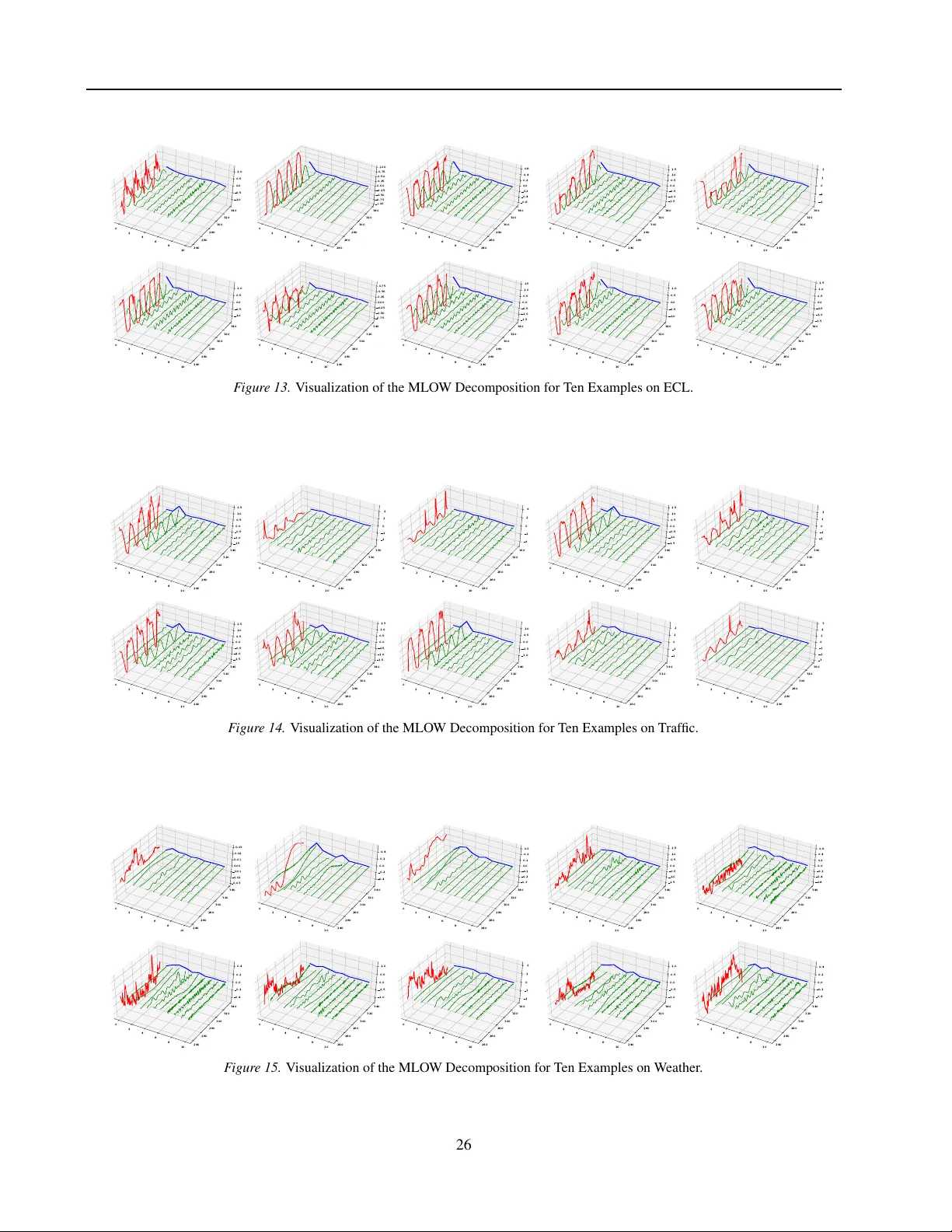
MLO W : Interpr etable Low-Rank Fr equency Magnitude Decomposition of Multiple Effects for T ime Series For ecasting Runze Y ang 1 2 Longbing Cao 1 Xiaoming W u 3 Xin Y ou 2 Kun F ang 4 Jianxun Li 2 Jie Y ang 2 https://github.com/runze1223/MLOW Abstract Separating multiple effects in time series is fun- damental yet challenging for time-series forecast- ing (TSF). Howe ver , existing TSF models can- not effecti vely learn interpretable multi-effect de- composition by their smoothing-based temporal techniques. Here, a ne w interpretable frequency- based decomposition pipeline MLOW captures the insight: a time series can be represented as a magnitude spectrum multiplied by the correspond- ing phase-aware basis functions, and the magni- tude spectrum distribution of a time series always exhibits observ able patterns for dif ferent effects. MLO W learns a lo w-rank representation of the magnitude spectrum to capture dominant trending and seasonal ef fects. W e e xplore low-rank meth- ods, including PCA, NMF , and Semi-NMF , and ﬁnd that none can simultaneously achieve inter- pretable, efﬁcient and generalizable decomposi- tion. Thus, we propose hyperplane-nonnegati ve matrix factorization (Hyperplane-NMF). Further , to address the frequency (spectral) leakage re- stricting high-quality low-rank decomposition, MLO W enables a ﬂexible selection of input hori- zons and frequency lev els via a mathematical mechanism. V isual analysis demonstrates that MLO W enables interpretable and hierarchical multiple-effect decomposition, robust to noises. It can also enable plug-and-play in e xisting TSF backbones with remarkable performance impro ve- ment but minimal architectural modiﬁcations. 1. Introduction T ime series forecasting (TSF) is fundamental for a wide range of real-w orld applications, such as demand prediction, 1 Macquarie Univ ersity 2 Shanghai Jiao T ong Univ ersity 3 Nanyang T echnological Univ ersity 4 Hong K ong Polytechnic Uni- versity . Correspondence to: Runze Y ang < runze.y@sjtu.edu.cn > . Pr eprint. Mar ch 20, 2026. Less Sensitive to Noise Hierarchical Effects (T rends) Frequency-based Low -Rank Multi-Effect Decomposition Hierarchical Effects (Seasonality) Traffic Observable Patterns PEMS03 Frequency M agnitude Spectrum ECL ETTh1 F igur e 1. The Motiv ation and V isualization for MLOW ﬁnancial risk assessment, climate and en vironmental moni- toring, industrial process control, and healthcare analytics ( Cao , 2020 ; 2023 ; Hong & Fan , 2016 ; Hyndman & Athana- sopoulos , 2018 ; Huang et al. , 2024 ). TSF requires ef fectiv e time series decomposition of multiple effects in time series, such as seasonality , trends, and residuals, crucial for inter- pretable TSF and do wnstream tasks. Ho we ver , ef fectiv ely decomposing a time series into meaningful trending, sea- sonal, and residual effects remains a fundamental challenge in comple x time series applications. It requires disentan- gling intertwined multi-effects, including trend dynamics, multi-scale seasonal patterns, and complex nonstationary ﬂuctuations in real-world time series. The decomposition module performs initial temporal disen- 1 MLO W : Interpr etable Low-Rank Fr equency Magnitude Decomposition of Multiple Effects for Time Series Forecasting tanglement before feeding the input into a TSF backbone. In e xisting deep TSF backbones, smoothing-based ﬁlters such as moving a verages serv e as the most widely used de- composition techniques, ﬁrstly introduced for Autoformer ( W u et al. , 2021 ). Although smoothing methods ha ve been commonly adopted by subsequent methods ( Zhou et al. , 2022b ; Zeng et al. , 2022 ; Cao et al. , 2023 ; W ang et al. , 2024 ; Shen et al. , 2024 ; Lin et al. , 2024b ; a ; Huang et al. , 2024 ), they are inherently sample-based. As a result, they are sensiti ve to noises, fail to disentangle different ef fects, and often produce inaccurate estimates at the boundaries due to padding. Consequently , these methods struggle to consistently enhance deep time series backbones b ut exhibit poor adaptability when applied to real-w orld TSF . How to achiev e interpretable and effecti ve multi-effect decomposi- tions remains an underexplored problem in TSF . While frequency-based methods attract increasing recent attention in TSF ( Zhou et al. , 2022a ; b ; Huang et al. , 2023 ; Y i et al. , 2023a ; W u et al. , 2022 ; Cao et al. , 2020 ; Y ang et al. , 2023a ; W ang et al. , 2025 ; Fei et al. , 2025 ; Y i et al. , 2024 ; Qiu et al. , 2025 ), they typically transform signals into fre- quency comple x values and rely on end-to-end supervised hidden state, which lack interpretability . In this work, we pursue interpretable frequency-based multi-ef fect decompo- sition beyond transforming with the follo wing insights. W e observe that the frequency magnitude spectrum distrib ution of a time series consistently exhibits observable patterns for different ef fects within the dataset, as illustrated in Figure 1 . T rending effects often exhibit an e xponentially decreasing pattern from low to high, while distinct seasonal effects typ- ically appear at multiple frequency le vels depending on the data granularity . The most prominent patterns usually cor- respond to the principal ef fects in a time series. Therefore, relying purely on high-, mid-, and low-frequenc y lev els is insufﬁcient for capturing multi-ef fects. In contrast, we propose MLO W which learns a lo w-rank representation of the frequency magnitude spectrum to cap- ture underlying patterns of principal trending and seasonal effects in time series. MLO W addresses the above gap and extends interpretability beyond frequenc y le vels to lo w-rank components. First, a sliding windo w ov er the training data obtains the samples. Then, we le verage the Fourier basis expansion ( Y ang et al. , 2024 ) to decompose all sample time series X into amplitudes R and phase-a ware basis functions B , aiming for learning a low-rank representation on their amplitudes. The amplitude, referring to frequency magni- tude spectrum, provides a valuable tool for analyzing time signals ( Zhang et al. , 2025 ; Y ang et al. , 2023b ), as it cap- tures the underlying effects in the signal. W e observe that all lo w-rank methods can be e xpressed as R = WH , where we refer H to the lo w-rank components and W as the ne w coefﬁcients for the low-rank components. Howe ver , this triggers two challenges. First, the existing lo w-rank meth- ods may not be well suited to magnitude spectrum. Second, the limited input horizon restricts the number of frequenc y lev els R that can be captured in a lo w-rank representation, leading to frequency (spectrum) leakage issues. T o address the ﬁrst challenge, we in vestigate e xisting de- composition methods for the magnitude spectrum. PCA ( Pearson , 1901 ) is one of the most widely used decomposi- tion methods, which suffers from a lo w interpretability , as it allows both lo w-rank components H and the corresponding coefﬁcient W takes negativ e values. This results in the decomposed components including negati ve combinations of phase-aware basis functions, which compromises the original phase effects. On the other hand, the non-negati ve matrix factorization (NMF) ( Lee & Seung , 1999 ) addresses the non-neg ativity issue, but it is computationally inef ﬁcient and not well generalizable to unseen data. The interpretabil- ity of W is also quite poor as it is based on ﬁtting. The Semi-NMF approach ( Ding et al. , 2008 ) faces same issues as PCA and NMF . T o ov ercome these challenges, we pro- pose a new lo w-rank method, namely Hyperplane-NMF for MLO W , where we force the W = RH T similar as the hyperplane projection by PCA while still follo wing the same principles as NMF with a cosine similarity penaliza- tion. Then, Hyperplane-NMF combines the advantages of the aforementioned methods to ensure the interpretability , efﬁcienc y and generalization of multi-effect decomposition. T o address the second challenge, a common issue in spectral analysis is the frequency (spectral) leakage. Speciﬁcally , when the number of av ailable frequency le vels is limited, the energy may spread across multiple frequency bins, which increases the dif ﬁculty of identifying prominent patterns. This is because the frequency le vel is constrained to half of the input horizon. T o ensure the decomposition independent of the input horizons with ﬂexible selection of frequency lev els, we introduce a mathematical mechanism. As shown in Figure 1 , we decompose time series into 10 low-ra nk pieces. The visualization indicates that the MLO W decomposition hierarchically separates distinct effects, with speciﬁc pieces more clearly representing trending and sea- sonal ef fects while exhibiting greater rob ustness to noises. The MLO W pipeline also of fers a clear interpretability for each piece and can characterize its source of energy . The empirical experiments also demonstrate that MLO W de- composition can remarkably improve e xisting TSF back- bones with minimal changes of their model architectures. T o summarize, both empirical results and visual evidence demonstrate the superiority of MLO W decomposition. The main contributions of this w ork include: • An interpretable decomposition pipeline to learn lo w- rank representations of the frequency magnitude distri- bution capturing multiple ef fects. 2 MLO W : Interpr etable Low-Rank Fr equency Magnitude Decomposition of Multiple Effects for Time Series Forecasting • A systematic in vestigation of strengths and weaknesses of three existing lo w-rank methods for magnitude spec- trum with ne w Hyperplane-NMF to combine their strengths for an interpretable, efﬁcient, and general- izable decomposition. • A mathematical mechanism that allo ws ﬂexible selec- tion of frequency le vels to compute the lo w-rank com- ponents independently of the input time horizons. 2. Related W orks 2.1. Low-Rank Repr esentation Learning PCA ( Pearson , 1901 ) can transform high-dimensional data to a smaller set of principal components while retaining most of the variances. It can identify the directions of maximum variances, which can sometimes uncover meaningful pat- terns. Howe ver , it produces negati ve values in the magnitude spectrum analysis, which are not interpretable as ne gativ e energy . In contrast, NMF ( Lee & Seung , 1999 ) can obtain a low-rank representation by constraining all components and coefﬁcients to be non-ne gativ e. Ho wev er , it is primarily designed for the matrix factorization rather than for efﬁ- cient and generalizable inference on ne w data. Semi-NMF ( Ding et al. , 2008 ) allo ws the corresponding coefﬁcients to take neg ativ e values while keeping the components positi ve but faces the same weakness as NMF . Nev ertheless, none of these methods can simultaneously satisfy the following three conditions: (i) both the components and correspond- ing coefﬁcients are non-ne gati ve for interpretability; (ii) no optimization is required when new data arrive, ensuring computational ef ﬁciency; and (iii) good generalizability and interpretability for W between the training and unseen data. Therefore, we de velop a ne w lo w-rank method tailored for magnitude-spectrum study . 2.2. TSF Model Backbone TSF backbones comprise popular DNN architectures in- cluding recurrent neural networks (RNNs) ( Hochreiter & Schmidhuber , 1997 ; Rangapuram et al. , 2018 ; Jia et al. , 2023 ; Salinas et al. , 2020 ; Kraus et al. , 2024 ), con volu- tion neural networks (CNNs) ( Luo & W ang , 2024 ; Liu et al. , 2022 ; W ang et al. , 2022 ; Franceschi et al. , 2019 ; Sen et al. , 2019 ), multi-layer perceptron (MLP) based net- works ( W ang et al. , 2024 ; Oreshkin et al. , 2019 ; Challu et al. , 2023 ; Y i et al. , 2023b ; Shi et al. , 2024 ; Xia et al. , 2025 ), and T ransformer-based networks ( Zhou et al. , 2022b ; 2021 ; W u et al. , 2021 ; Liu et al. , 2021 ; Zhang & Y an , 2022 ; Cao et al. , 2023 ; Fu et al. , 2024 ; Zhang et al. , 2023 ; Chen et al. , 2024 ; Liu et al. , 2024 ; Ma et al. , 2025 ; Qiu et al. , 2025 ). T o vali- date our decomposition method, we aim to select sophisti- cated models that require minimal architectural interv ention, limited to their initial projection layer . Accordingly , we select two most f amous and popular models, iT ransformer ( Liu et al. , 2024 ) and PatchTST ( Nie et al. , 2023 ), which satisfy this requirement. iTransformer introduces an initial projection from the time domain to the hidden state and uses the attention mechanism to capture channel interaction effects. PatchTST introduces an initial projection from the patched time series to the hidden state and uses the attention mechanism to model interactions between patches. Another reason we choose these two models is that they represent the most sophisticated independent and interaction-based architectures. 3. Methodology 3.1. Preliminaries MLO W aims for an interpretable multi-effect lo w-rank fre- quency magnitude decomposition to improve TSF . All de- compositions are initially computed inside the training, val- idation, and test data loaders, while the low-rank compo- nents H are obtained from the training data loader only . Since the initial projection in the TSF backbone is channel- independent, MLO W is also channel-independent. Thus, we discuss the decomposition in the univ ariate case for clarity . W e deﬁne an input time series X i ∈ R T paired with target Y i ∈ R L , where T as input horizon and L as forecast horizon. After applying MLOW on X i , we obtain the decomposed input ˙ X i = [ X i m , X i r , Z i ] | ˙ X i ∈ R ( T × ( V +2)) , where Z i is our V low-rank pieces (MLO W output), X i m and X i r refer to the mean intercept and the residual, respecti vely , both ha ving the same shape as X i . X i m is used for the normalization. Then, the de- composed V pieces and residuals are fed into the down- stream mapping network. T o minimize intervention in the downstream mapping and demonstrate its ef fectiv eness, we introduce only minimal modiﬁcations to the network ar- chitecture. Speciﬁcally , only the initial projection layer is modiﬁed for iTransformer and PatchTST . For iTrans- former , its initial projection layer nn.Linear ( T , g ) is re- placed by nn.Linear (( V + 1) × T , g ) . For P atchTST , its initial projection layer nn.Linear ( f , g ) is replaced by nn.Linear (( V + 1) × f , g ) . Here, T denotes the input length, f denotes the patch length, and g denotes the hidden dimension. Thus, the decompose time series is ﬂattened or ﬂattened after patching then fed into the initial projection layer for iT ransformer and P atchTST , respectiv ely . W e do the same inference to timestamps with same learned H for iT ransformer as they share the same initial projection layer . 3.2. MLO W’s Decomposition Pipeline and Challenges T o compute meaningful decompositions, W e distinguish dif- ferent ef fects (seasonal, and trending, etc.) by rearranging the same effects into a distinct low-rank component. In the frequency domain, the magnitude spectrum provides a 3 MLO W : Interpr etable Low-Rank Fr equency Magnitude Decomposition of Multiple Effects for Time Series Forecasting global overvie w of different ef fects, with distinct effects typically concentrated at separate frequency levels. Some energy at certain frequency le vels always tends to co-occur . Thus, we aim to learn a low-rank representation of the mag- nitude spectrum to capture most dominant ef fects by iden- tifying the underlying patterns of magnitude spectrum for each dataset. Thus, the decomposition pipeline is as follows: X i = R i B i + X i m , R i ∈ R K , B i ∈ R K × T (1) R i ≈ W i H , W ∈ R V , H ∈ R V × K , (2) P i = HB i , P ∈ R V × T , (3) Z i = W i ⊙ P i , Z i ∈ R V × T , (4) X i ≈ W i P i + X i m , X i r = X i − W i P i − X i m . (5) Let X i denote an input time series, with R i representing its amplitudes and B i the phase-aware bases from frequency lev el 1 to K , X i m is the mean intercept at frequency lev el 0 . H denotes low-rank components, with corresponding new coef ﬁcients W i , and the reconstructed bases are giv en by P i . First, we decompose the original time series into amplitude- and phase-aware basis functions. The ampli- tude, corresponding to the magnitude spectrum, serves as the coefﬁcient for the phase-aware basis functions. If a low-rank representation can accurately reconstruct the mag- nitude spectrum, it can also reconstruct the original time series well. Thus, the key is ho w to ﬁnd an interpretable, ef- ﬁcient and generalizable decomposition in Eq. ( 2 ) workable for any seen and unseen samples in a dataset. On the other, if the lev el of R is bounded for input horizon for X , but initially too low , it leads to frequency (spectral) leakage and makes ﬁnding quality lo w-rank components more difﬁcult. 3.3. Existing Low-Rank Methods vs Our Hyperplane-NMF Here, we aim to identify a low-rank method that is suit- able for the magnitude spectrum. Thus, we need to use the distrib ution of R i in the training set, as R ∈ R N × K , to obtain low rank components H . N is equal to the total number of sets i multiplied by the multiv ariate dimension D in the training set, since we mention that we use channel independence for MLOW . W e ﬁrst analyze the strengths and weaknesses of existing low-rank methods. Then, we introduce our Hyperplane-NMF method, follo wing the logic established in the in vestigation for e xisting methods. Finally , we explain why Hyperplane-NMF achie ves an interpretable, efﬁcient, and generalizable decomposition, and ho w it bene- ﬁts the downstream mapping netw ork. First, one of the most common dimensionality reduction methods is PCA. PCA usually requires subtracting the mean and dividing by the standard deviation before performing the transformation. Ho wev er , neither operation is appropri- ate here. The reason is intuitive: di viding by the standard deviation forces all frequenc y components to have the same scale, which is clearly not appropriate for making them equally important. Subtracting the mean remo ves the most important main features and leads to ne gativ e energy val- ues that are not interpretable. Thus, the PCA without the standardization is as follows: R = U Σ H , R ≈ U V Σ V H V , H V ∈ R V × K , W = U V Σ V = R H ⊤ V , R ≈ WH V . (6) The optimization of PCA is based on the SVD decomposi- tion. The strength of PCA is that it generalizes well to ne w data, as computing the coefﬁcient W for new samples is straightforward since it is simply a hyperplane projection R H ⊤ V . Ho wev er , its weaknesses are also apparent. The de- composition typically introduces negati ve v alues in both W and H . Negativ e values in H imply that the reconstructed bases P is formed through negati ve combinations of the orig- inal phase-a ware bases, while negati ve values in W indicate negati ve ener gy for the new reconstructed bases. Both com- promise the original phase-aw are information, making the decomposition less interpretable for magnitude spectrum. Second, NMF is also an effecti ve way to reduce dimen- sionality , especially for all positi ve matrix like magnitude spectrum. The optimization for NMF is as follo ws: min W , H ≥ 0 J ( W , H ) = 1 2 ∥R − WH ∥ 2 F , ∇ W J = WHH ⊤ − R H ⊤ , ∇ H J = W ⊤ WH − W ⊤ R , W ij ← W ij ( R H ⊤ ) ij ( WHH ⊤ ) ij , H ij ← H ij ( W ⊤ R ) ij ( W ⊤ WH ) ij . (7) The optimization is based on the EM algorithm, where W and H are optimized alternately . Since gradient descent may lead to negati ve values, multiplicati ve updates are used instead. Howe ver , this approach also faces sev eral issues. The ﬁrst issue is that it is not efﬁcient for unseen data: when new data arri ve, a ne w optimization problem must be solved. This is because, while we learn the low-rank components H from the training data, the corresponding coef ﬁcient W for the new data is unknown. Moreov er , since W is also non-negati ve, the least squares estimator cannot be applied. The optimization problem for new data is as follo ws: min W new ≥ 0 J ( W new ) = 1 2 ∥ R new − W new H ∥ 2 F . (8) The second limitation lies in its inferior generalization abil- ity relati ve to PCA, because adapting to new data requires 4 MLO W : Interpr etable Low-Rank Fr equency Magnitude Decomposition of Multiple Effects for Time Series Forecasting re-optimizing W , while W and H are jointly learned from the training set, thus the components H are optimized based on the particular W learned for the training data. The inter- preatability of W is also quite poor as it is based on ﬁtting. On the other hand, other methods like Semi-NMF f ace the same negativ e value issue as PCA and the generalization issue as NMF . More details can be found in Appendix. T able 1. Comparison for Lo w-Rank Methods: Hyperplane-NMF vs NMF , Semi-NMF , and PCA Hyperplane-NMF NMF Semi-NMF PCA Interpretable ✓ ✗ ✗ ✗ Efﬁcient for Ne w Data ✓ ✗ ✓ ✓ Generalizable for New Data ✓ ✗ ✗ ✓ Therefore, we propose the Hyperplane-NMF method to combine the strengths of existing approaches. Our method uses the same constraints as standard NMF decomposition, but enforces the coef ﬁcient matrix W = R H ⊤ , which represents a hyperplane projection, similar to PCA. The optimization process for Hyperplane-NMF is as follows: min W ≥ 0 , H ≥ 0 L ( W , H ) = ∥R − WH ∥ 2 F + λ X i  = j h ⊤ i h j ∥ h i ∥∥ h j ∥ , ∂ ∂ h i ∥R − R H ⊤ H ∥ 2 F = ( H R ⊤ )( R H ⊤ ) H − ( H R ⊤ ) R = W ⊤ WH − W ⊤ R , ∂ ∂ h i X j  = i h ⊤ i h j ∥ h i ∥ ∥ h j ∥ = X j  = i h j ∥ h i ∥ ∥ h j ∥ − X j  = i h ⊤ i h j ∥ h i ∥ 3 ∥ h j ∥ h i = ∇ + h i − ∇ − h i , W = R H ⊤ , H ← H ⊙ W ⊤ R + λ ∇ + H W ⊤ WH + λ ∇ − H . (9) There are three main adv antages of enforcing W = R H ⊤ . The ﬁrst advantage is that this formulation can be easily applied to new datasets without new optimization, as re- quired in the standard NMF . The second advantage is that, although the gradient itself does not change from the stan- dard NMF , it now points in the correct direction for the objectiv e, rather than tow ards a precomputed W at each iteration. Thus, the optimization constrains W to be com- puted via a h yperplane projection as a formalized rule in the objecti ve, which leads to impro ved generalization on unseen data. As mentioned before, the H of NMF are optimized based on particular ﬁtting W for the training data. Thirdly , the interpretability of W is superior to that of NMF , as it can be visualized through hyperplane projection rather than non-interpretable ﬁtting v alue. This pro vides a good inter - pretation of where the source of W comes from. In addition, to enforce greater di versity among the components of H , we further incorporate a Cosine similarity re gularization term with a regularized factor λ in our Hyperplane-NMF . This aims to identify the principal effects that are dif ferent from each other , with greater div ersity being preferable. As a result, Hyperplane-NMF is efﬁcient and generalizable to unseen data, making it highly ef fectiv e and interpretable for do wnstream mapping when applied to the validation or test dataset. In summary , Hyperplane-NMF offers a more interpretable, efﬁcient and generalizable decomposition. In T able 1 , we summarize the strengths of our Hyperplane- NMF compared with NMF , Semi-NMF , and PCA. 3.4. Flexible Frequency levels and Input Time Horizons In TSF , the lev els of the frequency magnitude are limited to T 2 + 1 of input horizon. When only a fe w frequency le vels are a vailable, the frequency spectrum is often too coarse to ﬁnd a good low-rank representation due to frequency (spectral) leakage. T o mitigate frequency (spectral) leakage, we want to achiev e ﬂexible frequency le vel selection. Thus, we use a longer historical windo w with length 2 K to e xtract the frequency spectrum, but only retain the most recent T segment of the resulting phase-aware basis functions for modeling. The mathematical formulation is as follo ws: X i = 1 2 K K X k =0 R i k cos  k π n K − φ k  = R i B i + X i m , R k = a k p r [ k ] 2 + i [ k ] 2 , φ k = atan2  i [ k ] , r [ k ]  , a k = ( 1 , k = 0 , K 2 , k = others n = 2 K − T + 1 , . . . , 2 K . (10) Here, r [ k ] and i [ k ] denote the frequency lev els at k of the real and imaginary parts, e xtracted by a windo w of length 2 K from X i w . This requires additional past information X i e , such that X i w = [ X i e , X i ] . Notably , X i e is not used in down- stream modeling, but only to boost the initial magnitude lev els. Since our ultimate goal is to compute a lo w-rank representation with rank V of the magnitude spectrum, in- creasing the initial lev els for magnitude spectrum at this stage does not affect the ﬁnal downstream mapping com- plexity . Thus, this mathematical dev elopment helps us b uild a ﬂexible pipeline to select both time horizon T and fre- quency le vel K freely . 3.5. Interpr etable Inference f or MLO W Decomposition More details for training and inference can be found in Ap- pendix Algorithm 1 . In Figure 2 , we visualize the inference pipeline of our method for its good interpretability . Here, after decomposition, both W and P are computed via a hy- perplane projection through lea ned H . Our method provides a clear and interpretable meaning for W and P , especially for W , helping understand its sources of energy . Commonly co-occurring patterns are more lik ely to be clustered into the 5 MLO W : Interpr etable Low-Rank Fr equency Magnitude Decomposition of Multiple Effects for Time Series Forecasting Flexible Frequency Level and Time Selection Learned Low Rank Components by Hyperplane-NMF K Levels Coefficients Reconstruct Basis Reconstruct Frequency-based Low-Rank Decomposition V components MLOW Output Difference for Residual Input Time Series Longer Window Magnitude Spectrum Phase-aware Basis Reconstructed Basis New Coefficients Interpretable Flexible Frequency Level Short-cut for T emporal (Eq.4) (Eq.1/10) F igur e 2. Infer ence pipeline for MLO W . The original time series is decomposed into V components and residual. A lar ger window for X enables more ﬂexible extraction of frequency magnitude levels while preserving the same temporal information.The learned Hyperplane-NMF components provide interpretable representations and serv e as interpretable sources for the decomposed pieces. same components, distinguishing them from others. In Fig- ure 3 , we visualize the learned components for the ECL data and observe se veral interesting patterns, where component weights are grouped by distinct frequency le vels. Compo- nents with grouped lo w-lev el weights, exhibiting an e xpo- nential decay pattern, more lik ely correspond to trending effects. Components with mid-level weights, which often activ ate multiples of speciﬁc frequency le vels, more lik ely correspond to seasonal effects. Components with high-le vel weights that exhibit jumps at certain frequency levels are more likely associated with nonstationary ﬂuctuations. For example, the y are visible in components 6, 7, and 8 in Fig- ure 3 . In particular, component 7 is extremely interesting, as it clusters the high le vels into one group while skipping certain lev els and assigning them to another component. This demonstrates that our decomposition can distinguish trending, seasonal and nonstationary effects in a more ef- fectiv e and interpretable manner . Thus, this explains why our decomposition looks more promising. In Figure 4 , the visualization sho ws that our MLOW decomposition is less sensitiv e to noises and can successfully separate trending and seasonal components hierarchically . W e provide more visualizations for decomposition and learned components for each data in Appendix. 4. Experiment Results 4.1. Datasets and Settings W e conduct our experiments on eight real-world datasets: ETTh1, Electricity (ECL), Traf ﬁc, W eather, and PEMS (PEMS04, PEMS08, PEMS03, PEMS07) ( Liu et al. , 2024 ). W e split the ETT datasets into 12/4/4 months for training, val idation, and test, respectiv ely , while all other datasets are split using a 0.7/0.1/0.2 ratio. W e extend the v alidation and test sets by the past window 2 K to ensure that their lengths are in variant. The dropout of last batch is disabled for the test set ( Qiu et al. , 2024 ). The forecasting horizons are ( 12 , 24 , 48 , 96 ) for short-term TSF on the PEMS datasets and ( 96 , 192 , 336 , 720 ) for long-term TSF on the other datasets, same as iT ransformer ( Liu et al. , 2024 ). W e ev aluate the plug-and-play performance on PatchTST and iT ransformer , and compare it with mo ving average (MA) decomposition with kernel size 24. The MA decomposition also modiﬁes only the ﬁrst initial projection layer for a fair comparison. All do wnstream mapping networks remain unchanged and use the same hyperparameters. The backbone hyperparame- ters are provided in T ables 11 and 12 in Appendix. F or the experiments in T ables 2 and 3 , we use the univ ersal same hyperparameters for MLO W: input sequence length T = 96 , frequency le vel K = 168 , number of low-rank components V = 10 , and regularization factor λ = 20 . 4.2. Main Results As shown in T able 2 , our method signiﬁcantly improves both P atchTST and iT ransformer to a ne w le vel, demonstrat- ing the ef fectiv eness of MLO W decomposition in separat- ing different effects for TSF . In contrast, moving-av erage kernels yield only marginal and often unstable improv e- ments. Our improv ement is robust for both long- and 6 MLO W : Interpr etable Low-Rank Fr equency Magnitude Decomposition of Multiple Effects for Time Series Forecasting 0 25 50 75 100 125 150 175 F r equency 0.0 0.2 0.4 0.6 0.8 1.0 1.2 1.4 Amplitude 95% CI Mean weight 0 25 50 75 100 125 150 175 F r equency 0.0 0.2 0.4 0.6 0.8 1.0 1.2 1.4 Amplitude 95% CI Mean weight 0 25 50 75 100 125 150 175 F r equency 0.0 0.2 0.4 0.6 0.8 1.0 1.2 1.4 Amplitude 95% CI Mean weight 0 25 50 75 100 125 150 175 F r equency 0.0 0.2 0.4 0.6 0.8 1.0 1.2 1.4 Amplitude 95% CI Mean weight 0 25 50 75 100 125 150 175 F r equency 0.0 0.2 0.4 0.6 0.8 1.0 1.2 1.4 Amplitude 95% CI Mean weight 0 25 50 75 100 125 150 175 F r equency 0.0 0.2 0.4 0.6 0.8 1.0 1.2 1.4 Amplitude 95% CI Mean weight 0 25 50 75 100 125 150 175 F r equency 0.0 0.2 0.4 0.6 0.8 1.0 1.2 1.4 Amplitude 95% CI Mean weight 0 25 50 75 100 125 150 175 F r equency 0.0 0.2 0.4 0.6 0.8 1.0 1.2 1.4 Amplitude 95% CI Mean weight 0 25 50 75 100 125 150 175 F r equency 0.0 0.2 0.4 0.6 0.8 1.0 1.2 1.4 Amplitude 95% CI Mean weight 0 25 50 75 100 125 150 175 F r equency 0.0 0.2 0.4 0.6 0.8 1.0 1.2 1.4 Amplitude 95% CI Mean weight F igur e 3. Learned 10 Components for the ECL Data Compared to Its Magnitude Spectrum Distributions. The blue regions correspond to the 95% conﬁdence interval of magnitude spectrum, the green columns show the mean magnitude spectrum, and the red columns indicate the weights of the learned components. The larger v ersion is shown in Figure 5 in the Appendix. 0 2 4 6 8 10 240 260 280 300 320 340 2 1 0 1 2 ECL 0 2 4 6 8 10 240 260 280 300 320 340 1.5 1.0 0.5 0.0 0.5 1.0 1.5 T rafﬁc 0 2 4 6 8 10 240 260 280 300 320 340 1.0 0.5 0.0 0.5 1.0 W eather 0 2 4 6 8 10 240 260 280 300 320 340 0.4 0.2 0.0 0.2 0.4 ETTh1 0 2 4 6 8 10 240 260 280 300 320 340 1.0 0.5 0.0 0.5 1.0 PEMS03 0 2 4 6 8 10 240 260 280 300 320 340 0.6 0.4 0.2 0.0 0.2 0.4 0.6 PEMS08 0 2 4 6 8 10 240 260 280 300 320 340 1.5 1.0 0.5 0.0 0.5 1.0 1.5 PEMS04 0 2 4 6 8 10 240 260 280 300 320 340 1.0 0.5 0.0 0.5 1.0 PEMS07 F igur e 4. V isualization of Our Decomposition on Eight Datasets. The results show that our decomposition can capture hierarchical ef fects. short-term TSF across all forecasting horizons. Over - all, iT ransformer+MLO W outperforms PatchTST+MLO W across most datasets, except ETTh1, as the separation of different effects allo ws interaction modeling to better cap- ture their relationships, especially in short-term TSF . In addition, we compare our ne w merged methods with other frequency-based and smoothing-based deep TSF methods on four datasets in T able 3 . The results sho w that iTrans- former+MLO W consistently achiev es the best performance and surpasses the second-best method by a large mar gin. 4.3. Ablation and Sensitivity Studies T able 4 also sho ws that our Hyperplane-NMF outperforms the other lo w-rank decomposed methods. Firstly , our method outperforms PCA because the proposed decom- position is strictly non-negati ve, thereby preserving the orig- inal phase-aw are information without introducing distortion. Secondly , it surpasses NMF as it exhibits stronger general- ization to unseen data. Our learned matrix W is also more interpretable than W obtained through optimization-based ﬁtting in NMF . In addition, incorporating Cosine similar - ity regularization also help impro ve NMF , encouraging the model to learn more div erse components. Finally , Semi- NMF performs worse than our method for the mentioned similar negati ve and generalizable reasons. T able 4 also shows that our lo w-rank method is much more ef ﬁcient than NMF decomposition, since the optimized for W is omitted. The inference time is measured on an ECL input sample with T = 96 , av eraged over 10 runs. T able 5 presents the sensiti vity studies using dif ferent lo w- 7 MLO W : Interpr etable Low-Rank Fr equency Magnitude Decomposition of Multiple Effects for Time Series Forecasting T able 2. MLO W vs. MA as Plug-and-Play Decomposition Modules on iT ransformer and PatchTST under T = 96 and the Same Hyperparameter . The full results are shown in T able 6 in Appendix. Methods iT ransformer+MLOW iT ransformer+MA iT ransformer PatchTST+MLO W PatchTST+MA PatchTST Error MSE MAE MSE MAE MSE MAE MSE MAE MSE MAE MSE MAE PEMS03 avg 0.086 0.186 0.130 0.232 0.129 0.233 0.108 0.222 0.203 0.297 0.214 0.307 PEMS04 avg 0.080 0.177 0.157 0.250 0.157 0.251 0.120 0.243 0.265 0.343 0.259 0.333 PEMS08 avg 0.081 0.173 0.142 0.233 0.142 0.232 0.120 0.232 0.221 0.313 0.221 0.308 PEMS07 avg 0.060 0.146 0.124 0.218 0.124 0.218 0.090 0.211 0.223 0.310 0.215 0.302 ECL avg 0.155 0.248 0.180 0.271 0.180 0.271 0.173 0.281 0.199 0.296 0.205 0.295 T rafﬁc a vg 0.393 0.250 0.417 0.280 0.428 0.282 0.405 0.294 0.470 0.309 0.467 0.309 W eather avg 0.231 0.264 0.259 0.280 0.261 0.282 0.232 0.263 0.255 0.278 0.253 0.277 ETTh1 avg 0.424 0.438 0.462 0.453 0.456 0.450 0.410 0.429 0.436 0.440 0.447 0.446 T able 3. MLOW + iT ransformer / PatchTST vs. Other Deep TSF Methods under T = 96. The full results are in T able 7 in Appendix. Methods iTransformer+MLO W PatchTST+MLO W DUET CycleNet SparseTSF T imeKAN T imesNet TimeMix er ( Liu et al. , 2024 ) ( Nie et al. , 2023 ) ( Qiu et al. , 2025 ) ( Lin et al. , 2024a ) ( Lin et al. , 2024b ) ( Huang et al. , 2024 ) ( Wu et al. , 2022 ) ( W ang et al. , 2024 ) Error MSE MAE MSE MAE MSE MAE MSE MAE MSE MAE MSE MAE MSE MAE MSE MAE PEMS03 avg 0.086 0.186 0.108 0.222 0.114 0.223 0.122 0.223 0.297 0.352 0.276 0.3465 0.149 0.257 0.107 0.212 PEMS08 avg 0.081 0.173 0.120 0.232 0.104 0.211 0.150 0.237 0.298 0.351 0.275 0.346 0.189 0.280 0.120 0.225 ECL avg 0.155 0.248 0.173 0.281 0.172 0.258 0.167 0.259 0.214 0.288 0.203 0.292 0.192 0.295 0.182 0.272 Traf ﬁc avg 0.393 0.250 0.405 0.294 0.451 0.269 0.471 0.301 0.589 0.339 0.577 0.372 0.619 0.335 0.484 0.297 T able 4. Performance of MLOW with Different Lo w-Rank Meth- ods on iTransformer and A verage Inference T ime for an Input T ime Series on ECL. The full results are in T able 8 in Appendix. Methods Hyperplane-NMF NMF PCA Semi-NMF Error MSE MAE MSE MAE MSE MAE MSE MAE PEMS08 avg 0.081 0.173 0.083 0.175 0.086 0.177 0.089 0.184 ECL avg 0.155 0.248 0.163 0.258 0.160 0.255 0.166 0.260 Inference Time (s) 0.000259 0.121408 0.000265 0.000288 rank values of V for the initial frequency lev els K = 168 and K = 48 , respecti vely . Small values of V make little difference while V = 5 or V = 10 usually enables optimal, and continuously increasing V does not necessarily improv e performance; in fact, it often degrades it. This is because our ultimate goal is to separate different ef fects, and the large V components may confuse the model for different effects. Howe ver , using K = 168 consistently yields better results than K = 48 under the same V , ev en though model architectures are identical. This shows that our mathematical mechanism in Section 3.4 is v ery important; otherwise, K can only equal T 2 . This is because extra levels for K mitigate the frequency (spectral) leakage ef fects to help ﬁnd a better low-rank decomposition. 5. Conclusions The interpretability of our MLO W decomposition draws the following perspectiv es: (i) the low-rank pieces visual- ization shows that our decomposition separates dif ferent T able 5. Sensitivity Analysis for K and V on iT ransformer . The full results are provided in T able 9 in Appendix. Error MSE MAE MSE MAE MSE MAE MSE MAE (K=168) V=5 V=10 V=15 V=20 PEMS08 avg 0.082 0.173 0.081 0.173 0.081 0.173 0.082 0.174 ECL avg 0.154 0.246 0.155 0.248 0.155 0.248 0.156 0.251 (K=48) V=5 V=10 V=15 V=20 PEMS08 avg 0.086 0.182 0.087 0.183 0.087 0.182 0.088 0.184 ECL avg 0.161 0.252 0.160 0.251 0.161 0.253 0.162 0.253 effects hierarchically and is robust to noise; (ii) the low- rank components provide a meaningful source of W and P by grouping certain frequency le vels; (iii) the learned low-rank components are strictly positiv e and div erse. The empirical results also sho w that our decomposition improves iT ransformer and PatchTST by only adjusting the initial pro- jection layer , which has minimal inﬂuence on the model architecture but yields a remarkable improv ement on fore- casting performance. With MLO W serving as an initial interpretable decomposition, it pushes existing TSF models to a new le vel. Thus, our method provides a new path for interpretable TSF . Our decomposition is also highly efﬁ- cient for inference and can be readily applied in real-world scenarios. One limitation is that the optimal rank of V is not univ ersally ﬁxed for each dataset. Thus, our future work will explore de velopments that enable low-rank methods to as- sign importance scores to the learned components. W e also plan to in vestigate the application of MLO W in other time series tasks, such as anomaly detection and classiﬁcation. 8 MLO W : Interpr etable Low-Rank Fr equency Magnitude Decomposition of Multiple Effects for Time Series Forecasting Acknowledgements This research is partially supported by NSFC (No. 62376153), and ARC Grants DP240102050, DP260104429, LP230201022 and LE240100131. Impact Statement MLO W represents a new interpretable low-rank frequenc y magnitude decomposition approach for time series forecast- ing. By separating principal trending and seasonal ef fects, MLO W can substantially enhance both interpretability and predictiv e performance of any TSF backbones with only minimal changes required to their underlying model archi- tectures. It can transform TSF in applications such as energy demand prediction, trafﬁ c forecasting, and en vironmental monitoring, where characterizing distinct time series effects is essential yet challenging. The MLO W interpretability en- ables a better analysis of temporal patterns for trustw orthy modeling of complex beha viors. References Cao, D., W ang, Y ., Duan, J., Zhang, C., Zhu, X., Huang, C., T ong, Y ., Xu, B., Bai, J., T ong, J., et al. Spectral tem- poral graph neural network for multivariate time-series forecasting. Advances in neural information pr ocessing systems , 33:17766–17778, 2020. Cao, H., Huang, Z., Y ao, T ., W ang, J., He, H., and W ang, Y . InParformer: ev olutionary decomposition transformers with interactive parallel attention for long-term time series forecasting. In AAAI Confer ence on Artiﬁcial Intelligence , 2023. Cao, L. AI in ﬁnance: A revie w . SSRN , pp. 1– 36, 2020. URL http://dx.doi.org/10.2139/ ssrn.3647625 . Cao, L. AI in ﬁnance: Challenges, techniques, and opportu- nities. ACM Comput. Surv . , 55(3):64:1–64:38, 2023. Challu, C., Oliv ares, K. G., Oreshkin, B. N., Ramirez, F . G., Canseco, M. M., and Dubrawski, A. N-HiTS: Neural hierarchical interpolation for time series forecasting. In AAAI Confer ence on Artiﬁcial Intelligence , volume 37, pp. 6989–6997, 2023. Chen, P ., Zhang, Y ., Cheng, Y ., Shu, Y ., W ang, Y ., W en, Q., Y ang, B., and Guo, C. Pathformer: Multi-scale transform- ers with adapti ve pathways for time series forecasting. arXiv pr eprint arXiv:2402.05956 , 2024. Ding, C. H., Li, T ., and Jordan, M. I. Con vex and semi- nonnegati ve matrix f actorizations. IEEE transactions on pattern analysis and mac hine intelligence , 32(1):45–55, 2008. Fei, J., Y i, K., Fan, W ., Zhang, Q., and Niu, Z. Ampliﬁer: Bringing attention to neglected lo w-energy components in time series forecasting. In AAAI Confer ence on Artiﬁcial Intelligence , 2025. Franceschi, J.-Y ., Dieulev eut, A., and Jaggi, M. Unsuper- vised scalable representation learning for multi variate time series. Advances in Neural Information Pr ocessing Systems , 32, 2019. Fu, K., Li, H., and Shi, X. An encoder–decoder architecture with fourier attention for chaotic time series multi-step prediction. Applied Soft Computing , pp. 111409, 2024. Hochreiter , S. and Schmidhuber , J. Long short-term memory . Neural computation , 9(8):1735–1780, 1997. Hong, T . and Fan, S. Probabilistic electric load forecasting: A tutorial revie w . International Journal of F or ecasting , 32(3):914–938, 2016. Huang, Q., Shen, L., Zhang, R., Ding, S., W ang, B., Zhou, Z., and W ang, Y . Crossgnn: Confronting noisy multi- variate time series via cross interaction reﬁnement. Ad- vances in Neural Information Pr ocessing Systems , 36: 46885–46902, 2023. Huang, S., Zhao, Z., Li, C., and BAI, L. T imekan: Kan- based frequency decomposition learning architecture for long-term time series forecasting. In International Con- fer ence on Learning Repr esentations , 2024. Hyndman, R. J. and Athanasopoulos, G. F or ecasting: prin- ciples and practice . OT exts, 2018. Jia, Y ., Lin, Y ., Hao, X., Lin, Y ., Guo, S., and W an, H. W itran: W ater-wa ve information transmission and re- current acceleration network for long-range time series forecasting. Advances in Neural Information Pr ocessing Systems , 36:12389–12456, 2023. Kraus, M., Di vo, F ., Dhami, D. S., and Kersting, K. xlstm- mixer: Multiv ariate time series forecasting by mixing via scalar memories. arXiv preprint , 2024. Lee, D. D. and Seung, H. S. Learning the parts of objects by non-negati ve matrix f actorization. nature , 401(6755): 788–791, 1999. Lin, S., Lin, W ., Hu, X., W u, W ., Mo, R., and Zhong, H. Cyclenet: Enhancing time series forecasting through mod- eling periodic patterns. Advances in Neural Information Pr ocessing Systems , 37:106315–106345, 2024a. Lin, S., Lin, W ., W u, W ., Chen, H., and Y ang, J. Sparsetsf: modeling long-term time series forecasting with 1k pa- rameters. In International Confer ence on Machine Learn- ing , pp. 30211–30226, 2024b. 9 MLO W : Interpr etable Low-Rank Fr equency Magnitude Decomposition of Multiple Effects for Time Series Forecasting Liu, M., Zeng, A., Chen, M., Xu, Z., Lai, Q., Ma, L., and Xu, Q. Scinet: T ime series modeling and forecasting with sample con volution and interaction. Advances in Neural Information Pr ocessing Systems , 35:5816–5828, 2022. Liu, S., Y u, H., Liao, C., Li, J., Lin, W ., Liu, A. X., and Dustdar , S. Pyraformer: Low-comple xity pyramidal atten- tion for long-range time series modeling and forecasting. In International confer ence on learning r epr esentations , 2021. Liu, Y ., Hu, T ., Zhang, H., W u, H., W ang, S., Ma, L., and Long, M. iTransformer: Inv erted transformers are effecti ve for time series forecasting. In International Confer ence on Learning Repr esentations , 2024. Luo, D. and W ang, X. ModernTCN: A modern pure con- volution structure for general time series analysis. In International Confer ence on Learning Representations , pp. 1–43, 2024. Ma, J., W ang, B., Huang, Q., W ang, G., W ang, P ., Zhou, Z., and W ang, Y . Mofo: Empo wering long-term time series forecasting with periodic pattern modeling. In Advances in Neural Information Pr ocessing Systems , 2025. Nie, Y ., Nguyen, N. H., Sinthong, P ., and Kalagnanam, J. A time series is worth 64 words: Long-term forecasting with transformers. In International Confer ence on Learning Repr esentations , 2023. Oreshkin, B. N., Carpov , D., Chapados, N., and Bengio, Y . N-beats: Neural basis expansion analysis for interpretable time series forecasting. arXiv pr eprint arXiv:1905.10437 , 2019. Pearson, K. Liii. on lines and planes of closest ﬁt to systems of points in space. The London, Edinbur gh, and Dublin philosophical magazine and journal of science , 2(11): 559–572, 1901. Qiu, X., Hu, J., Zhou, L., W u, X., Du, J., Zhang, B., Guo, C., Zhou, A., Jensen, C. S., Sheng, Z., et al. Tfb: T owards comprehensi ve and fair benchmarking of time series fore- casting methods. arXiv preprint , 2024. Qiu, X., W u, X., Lin, Y ., Guo, C., Hu, J., and Y ang, B. Duet: Dual clustering enhanced multiv ariate time series forecasting. In ACM SIGKDD Confer ence on Knowledge Discovery and Data Mining , 2025. Rangapuram, S. S., Seeger , M. W ., Gasthaus, J., Stella, L., W ang, Y ., and Januschowski, T . Deep state space models for time series forecasting. Advances in Neural Information Pr ocessing Systems , 31, 2018. Salinas, D., Flunk ert, V ., Gasthaus, J., and Januschowski, T . Deepar: Probabilistic forecasting with autore gressiv e recurrent networks. International Journal of F or ecasting , 36(3):1181–1191, 2020. Sen, R., Y u, H.-F ., and Dhillon, I. S. Think globally , act locally: A deep neural network approach to high- dimensional time series forecasting. Advances in Neural Information Pr ocessing Systems , 32, 2019. Shen, L., Chen, W ., and Kwok, J. Multi-resolution diffu- sion models for time series forecasting. In International Confer ence on Learning Repr esentations , 2024. Shi, X., W ang, S., Nie, Y ., Li, D., Y e, Z., W en, Q., and Jin, M. Time-moe: Billion-scale time series founda- tion models with mixture of experts. arXiv preprint arXiv:2409.16040 , 2024. W ang, H., Peng, J., Huang, F ., W ang, J., Chen, J., and Xiao, Y . MICN: Multi-scale local and global context model- ing for long-term series forecasting. In International Confer ence on Learning Repr esentations , 2022. W ang, H., Pan, L., Chen, Z., Y ang, D., Zhang, S., Y ang, Y ., Liu, X., Li, H., and T ao, D. Fredf: Learning to forecast in the frequency domain. In International Conference on Learning Repr esentations , 2025. W ang, S., W u, H., Shi, X., Hu, T ., Luo, H., Ma, L., Zhang, J. Y ., and Zhou, J. T imeMixer: Decomposable multi- scale mixing for time series forecasting. International Confer ence on Learning Repr esentations , 2024. W u, H., Xu, J., W ang, J., and Long, M. Autoformer: Decom- position transformers with auto-correlation for long-term series forecasting. Advances in Neural Information Pr o- cessing Systems , 34:22419–22430, 2021. W u, H., Hu, T ., Liu, Y ., Zhou, H., W ang, J., and Long, M. T imesNet: T emporal 2d-v ariation modeling for gen- eral time series analysis. In International Conference on Learning Repr esentations , 2022. Xia, M., Zhang, C., Zhang, Z., Miao, H., Liu, Q., Zhu, Y ., and Y ang, B. T imeemb: A lightweight static-dynamic disentanglement framew ork for time series forecasting. arXiv pr eprint arXiv:2510.00461 , 2025. Y ang, F ., Li, X., W ang, M., Zang, H., P ang, W ., and W ang, M. W a veform: Graph enhanced wa velet learning for long sequence forecasting of multiv ariate time series. In AAAI confer ence on artiﬁcial intelligence , 2023a. Y ang, R., Lv , K., Huang, Y ., Sun, M., Li, J., and Y ang, J. Respiratory sound classiﬁcation by applying deep neu- ral network with a blocking v ariable. Applied Sciences , 2023b. 10 MLO W : Interpr etable Low-Rank Fr equency Magnitude Decomposition of Multiple Effects for Time Series Forecasting Y ang, R., Cao, L., Y ANG, J., et al. Rethinking fourier trans- form from a basis functions perspectiv e for long-term time series forecasting. Advances in Neural Information Pr ocessing Systems , 37:8515–8540, 2024. Y i, K., Zhang, Q., F an, W ., He, H., Hu, L., W ang, P ., An, N., Cao, L., and Niu, Z. FourierGNN: Rethinking multi vari- ate time series forecasting from a pure graph perspective. arXiv pr eprint arXiv:2311.06190 , 2023a. Y i, K., Zhang, Q., Fan, W ., W ang, S., W ang, P ., He, H., An, N., Lian, D., Cao, L., and Niu, Z. Frequency-domain mlps are more ef fectiv e learners in time series forecasting. Advances in Neural Information Pr ocessing Systems , 36: 76656–76679, 2023b. Y i, K., Fei, J., Zhang, Q., He, H., Hao, S., Lian, D., and F an, W . Filternet: Harnessing frequency ﬁlters for time series forecasting. Advances in Neural Information Pr ocessing Systems , 37:55115–55140, 2024. Zeng, A., Chen, M., Zhang, L., and Xu, Q. Are transformers effecti ve for time series forecasting? arXiv preprint arXiv:2205.13504 , 2022. Zhang, Q., Sun, Y ., W en, H., Y ang, P ., Li, X., Li, M., Lam, K.-Y ., Y iu, S.-M., and Y in, H. Time series analysis in frequency domain: A surve y of open chal- lenges, opportunities and benchmarks. arXiv pr eprint arXiv:2504.07099 , 2025. URL https://arxiv. org/abs/2504.07099 . Zhang, Y . and Y an, J. Crossformer: T ransformer utilizing cross-dimension dependency for multi variate time series forecasting. In International Conference on Learning Repr esentations , 2022. Zhang, Z., Han, Y ., Ma, B., Liu, M., and Geng, Z. T em- poral chain network with intuitiv e attention mechanism for long-term series forecasting. IEEE T ransactions on Instrumentation and Measur ement , 2023. Zhou, H., Zhang, S., Peng, J., Zhang, S., Li, J., Xiong, H., and Zhang, W . Informer: Beyond efﬁcient transformer for long sequence time-series forecasting. In AAAI Con- fer ence on Artiﬁcial Intelligence , volume 35, pp. 11106– 11115, 2021. Zhou, T ., Ma, Z., W en, Q., Sun, L., Y ao, T ., Y in, W ., Jin, R., et al. FiLM: Frequency impro ved le gendre memory model for long-term time series forecasting. Advances in Neural Information Pr ocessing Systems , 35:12677– 12690, 2022a. Zhou, T ., Ma, Z., W en, Q., W ang, X., Sun, L., and Jin, R. Fedformer: Frequency enhanced decomposed trans- former for long-term series forecasting. In International Confer ence on Machine Learning , pp. 27268–27286. PMLR, 2022b. 11 MLO W : Interpr etable Low-Rank Fr equency Magnitude Decomposition of Multiple Effects for Time Series Forecasting A. MLO W T raining and Inference Process W e provide a more detail training and inference process in Algorithm 1 . W e use a univ ersal ﬁx ed random seed in the released source codes so that you can reproduce exactly the same components showing in the manuscript. The uni versal parameters for MLO W are the total number of iterations F = 1000 , input sequence length T = 96 , frequency le vel K = 168 , number of lo w-rank components V = 10 , and regularization weight λ = 20 . The downstream mapping network uses the same learned H as presented in the manuscript, av eraged over tw o runs for the results in the table. B. Low-Rank Decomposition by Semi-NMF W e introduce another lo w-rank method called Semi-NMF , which only requires H to be non-ne gativ e. Its optimization formula is as follows: min H ≥ 0 J ( W , H ) = 1 2 ∥R − WH ∥ 2 F , W = R H ⊤ ( HH ⊤ ) − 1 , H ij ← H ij ([ W ⊤ R ] ij ) + + H ij ([ W ⊤ WH ] ij ) − ([ W ⊤ R ] ij ) − + H ij ([ W ⊤ WH ] ij ) + , A + = max( A , 0) , A − = max( − A , 0) . (11) The only strength of this method is that it is relativ ely efﬁcient for new data, as W can be directly computed through the least square estimator . Howe ver , its weakness is similar to PCA, that negati ve coef ﬁcients compromise the phase-aware temporal information. In addition, although W can be directly computed using least squares. The optimization would, in principle, be simpler , it fails to conv erge properly since the gradient does not correctly direct to the objective. This is because ( HH ⊤ ) − 1 is unstable and can change quite dramatically , which leads to the optimization for H being unstable. The gradient is computed with respect to W at the current iteration, rather than the true gradient of the objectiv e. C. T ables The full results for T ables 2 , 3 , 4 and 5 are provided in T ables 6 , 7 , 8 and 9 , respectiv ely . T able 10 provides more details for data description. The training details for iTransformer and PatchTST are provided in T ables 11 and 12 , and the hyperparameters for MLO W hav e already been mentioned in the manuscript. D. V isualization Figures 5 and 6 provide the visualization for the learned weights of 10 components for the ECL and Traf ﬁc data. These datasets include more seasonal effects than trending effects. Thus, this corresponds to more patternable weights across multiple components because speciﬁc seasonal effects are more likely to be seen at multiple lev els. W e also ﬁnd exponentially deceasing weights from low to high here. On the other hand, Figure 7 and 8 provide visualization of the learned weights of 10 components for the W eather and ETTh1 datasets. W e observ e a number of interesting patterns. In particular , the weather dataset exhibits many trending effects, resulting in the learned components to show the most pronounced exponentially decaying behaviors. W e further observe that multiple components e xhibit similar , patternable weight structures around the peaks of the magnitude distribution in the ETTh1 dataset. Figures 9 , 10 , 11 , and 12 provide the visualization for the learned weights of 10 components for datasets PEMS03, PEMS04, PEMS07, PEMS08. These data sets include more trending effects than seasonal ef fects, but we also observe small peak at multiple frequency le vels. Our learned weights exhibit both exponential decay patterns, such as components 9, 6, 7, and 7 for PEMS03, PEMS04, PEMS07, and PEMS08, respectiv ely , and peak-concentrated patterns, such as components 7, 8, and 8 for PEMS04, PEMS07, and PEMS08, respecti vely . In conclusion, magnitude lev els that tend to co-occur with high energy in observable patterns are more likely to be in the same components. Figures 13 14 15 , 16 , 17 , 18 , 19 , and 20 provide ten examples of MLO W decomposition for ECL, T rafﬁc, W eather , ETTh1, PEMS03, PEMS08, PEMS04, and PEMS07, respectiv ely , with the ﬁrst ﬁv e from the training sets and the last ﬁ ve from v alidation and test sets. These results demonstrate that our MLO W method can produce more interpretable decompositions by disentangling different ef fects and remaining robust to noises. 12 MLO W : Interpr etable Low-Rank Fr equency Magnitude Decomposition of Multiple Effects for Time Series Forecasting Algorithm 1 MLO W : Low-Rank Frequenc y Magnitude Decomposition Require: V alid time series sample R ∈ R N × K extracted by X ∈ R N × 2 K , frequency le vels K , low-rank representation V , the number of iterations F , the length of training set I , the number of multi variate D , regularized f actor λ , input sequence length T . Ensure: The total valid number of frequency spectrum samples N = ( I − 2 K ) × D , co vering all v alid amplitude extraction instances in the training dataset. This is achie ved by a windo w 2 K sliding ov er the training data. T raining Phase: Compute frequency spectrum R by Eq. (1) in the manuscript for all valid samples. Initialize low-rank factors H ∈ R V × K with top v eigen vectors of the PCA, b ut the negati ve values are replaced by random positi ve v alues. This is because our hyperplane projection is the same as PCA, b ut we don’t allo w neg ativ e values. Force the corresponding coef ﬁcient W = R H T . for i = 1 to F do Update H by Eq. (9) in the manuscript. end for Obtained leaned low-rank components H . Inference Phase: This is required when 2 K is larger than T . F or an input time series X i with time horizon T , we extend the input horizon to 2 K to extract the magnitude spectrum by X i w = [ X i e , X i ] ∈ R 2 K , then we express it as X i w = R i B i w , while only the last T timestamps in B i w are used as the ef fectiv e temporal information. Thus, we only take B i of B i w = [ B i e , B i ] as the phase-aw are bases we need. All the windo ws here contain strictly past information and do not include an y forecast horizon. Obtain the X i = R i B i + X i m by Eq. (10) in the manuscript. Compute the new coef ﬁcient W i = R i H T . Compute the new reconstructed basis P i = HB i . Obtain the low-rank decomposition Z i = W i ⊙ P i . Obtain the residual X i r = X i − W i P i − X i m . Do the same for timestamps decomposition if timestamps are required. This is because, in the initial iTransformer setting, the timestamps share the same initial projection weights. 13 MLO W : Interpr etable Low-Rank Fr equency Magnitude Decomposition of Multiple Effects for Time Series Forecasting T able 6. MLO W vs. MA as Plug-and-Play Decomposition Modules on iT ransformer and PatchTST under T = 96 and the Same Hyperparameter . Methods iT ransformer+Ours iT ransformer+MA iTransformer PatchTST+Ours PatchTST+MA PatchTST Error MSE MAE MSE MAE MSE MAE MSE MAE MSE MAE MSE MAE PEMS03 12 0.064 0.164 0.064 0.167 0.067 0.169 0.079 0.194 0.094 0.208 0.105 0.227 24 0.078 0.179 0.091 0.199 0.090 0.199 0.096 0.209 0.146 0.258 0.157 0.271 48 0.093 0.196 0.145 0.250 0.142 0.250 0.117 0.230 0.220 0.316 0.234 0.325 96 0.109 0.208 0.220 0.315 0.218 0.315 0.142 0.255 0.353 0.406 0.362 0.405 avg 0.086 0.186 0.130 0.232 0.129 0.233 0.108 0.222 0.203 0.297 0.214 0.307 PEMS04 12 0.067 0.163 0.083 0.183 0.085 0.187 0.089 0.213 0.112 0.234 0.112 0.227 24 0.075 0.172 0.113 0.214 0.113 0.214 0.104 0.230 0.174 0.288 0.165 0.278 48 0.084 0.182 0.171 0.268 0.170 0.267 0.132 0.254 0.303 0.376 0.283 0.359 96 0.096 0.192 0.262 0.336 0.262 0.338 0.156 0.278 0.474 0.476 0.477 0.469 avg 0.080 0.177 0.157 0.250 0.157 0.251 0.120 0.243 0.265 0.343 0.259 0.333 PEMS08 12 0.065 0.158 0.071 0.168 0.072 0.170 0.088 0.207 0.106 0.227 0.099 0.220 24 0.074 0.167 0.102 0.204 0.099 0.200 0.106 0.221 0.169 0.285 0.174 0.287 48 0.087 0.180 0.157 0.250 0.155 0.248 0.129 0.241 0.238 0.328 0.229 0.322 96 0.099 0.187 0.241 0.312 0.243 0.311 0.160 0.260 0.374 0.413 0.382 0.406 avg 0.081 0.173 0.142 0.233 0.142 0.232 0.120 0.232 0.221 0.313 0.221 0.308 PEMS07 12 0.050 0.135 0.064 0.159 0.065 0.160 0.070 0.190 0.093 0.217 0.089 0.206 24 0.056 0.143 0.092 0.189 0.092 0.191 0.080 0.202 0.141 0.259 0.136 0.254 48 0.064 0.151 0.140 0.237 0.139 0.236 0.096 0.217 0.253 0.338 0.242 0.329 96 0.071 0.158 0.203 0.289 0.202 0.288 0.117 0.235 0.407 0.429 0.393 0.420 avg 0.060 0.146 0.124 0.218 0.124 0.218 0.090 0.211 0.223 0.310 0.215 0.302 ECL 96 0.130 0.223 0.151 0.245 0.151 0.245 0.144 0.255 0.171 0.273 0.176 0.271 192 0.149 0.240 0.167 0.259 0.167 0.259 0.161 0.271 0.182 0.281 0.188 0.282 336 0.162 0.256 0.182 0.276 0.185 0.276 0.176 0.284 0.200 0.298 0.203 0.297 720 0.181 0.276 0.220 0.307 0.217 0.304 0.212 0.316 0.244 0.333 0.254 0.333 avg 0.155 0.248 0.180 0.271 0.180 0.271 0.173 0.281 0.199 0.296 0.205 0.295 T rafﬁc 96 0.353 0.229 0.395 0.266 0.395 0.268 0.372 0.278 0.445 0.297 0.440 0.295 192 0.380 0.241 0.412 0.276 0.417 0.276 0.393 0.287 0.457 0.303 0.454 0.303 336 0.402 0.251 0.417 0.284 0.433 0.283 0.409 0.296 0.473 0.310 0.469 0.310 720 0.438 0.266 0.444 0.295 0.467 0.302 0.446 0.315 0.508 0.327 0.508 0.328 avg 0.393 0.250 0.417 0.280 0.428 0.282 0.405 0.294 0.470 0.309 0.467 0.309 W eather 96 0.155 0.201 0.173 0.215 0.178 0.218 0.154 0.199 0.174 0.217 0.173 0.216 192 0.196 0.242 0.226 0.259 0.223 0.256 0.198 0.240 0.220 0.257 0.218 0.255 336 0.246 0.280 0.281 0.298 0.281 0.298 0.249 0.280 0.277 0.296 0.275 0.295 720 0.330 0.334 0.359 0.350 0.363 0.359 0.330 0.334 0.350 0.343 0.348 0.342 avg 0.231 0.264 0.259 0.280 0.261 0.282 0.232 0.263 0.255 0.278 0.253 0.277 ETTh1 96 0.375 0.404 0.392 0.409 0.390 0.407 0.369 0.398 0.384 0.402 0.389 0.409 192 0.416 0.431 0.443 0.439 0.443 0.439 0.413 0.425 0.427 0.432 0.430 0.436 336 0.439 0.443 0.491 0.464 0.488 0.462 0.423 0.432 0.460 0.451 0.471 0.454 720 0.466 0.475 0.524 0.500 0.504 0.492 0.438 0.462 0.474 0.475 0.500 0.486 avg 0.424 0.438 0.462 0.453 0.456 0.450 0.410 0.429 0.436 0.440 0.447 0.446 14 MLO W : Interpr etable Low-Rank Fr equency Magnitude Decomposition of Multiple Effects for Time Series Forecasting T able 7. MLOW + iT ransformer / PatchTST vs. Other Deep TSF Methods under T = 96. Methods iTransformer+MLO W P atchTST+MLOW DUET CycleNet SparseTSF TimeKAN T imesNet TimeMix er ( Liu et al. , 2024 ) ( Nie et al. , 2023 ) ( Qiu et al. , 2025 ) ( Lin et al. , 2024a ) ( Lin et al. , 2024b ) ( Huang et al. , 2024 ) ( W u et al. , 2022 ) ( W ang et al. , 2024 ) Error MSE MAE MSE MAE MSE MAE MSE MAE MSE MAE MSE MAE MSE MAE MSE MAE PEMS03 12 0.064 0.164 0.079 0.194 0.065 0.169 0.066 0.170 0.116 0.230 0.099 0.211 0.083 0.191 0.063 0.164 24 0.078 0.179 0.096 0.209 0.089 0.197 0.092 0.201 0.173 0.282 0.163 0.268 0.125 0.234 0.080 0.187 48 0.093 0.196 0.117 0.230 0.130 0.242 0.141 0.245 0.328 0.388 0.319 0.388 0.160 0.270 0.114 0.226 96 0.109 0.208 0.142 0.255 0.172 0.285 0.189 0.279 0.571 0.508 0.523 0.519 0.231 0.333 0.174 0.273 avg 0.086 0.186 0.108 0.222 0.114 0.223 0.122 0.223 0.297 0.352 0.276 0.3465 0.149 0.257 0.107 0.212 PEMS08 12 0.065 0.158 0.088 0.207 0.068 0.167 0.080 0.181 0.121 0.231 0.099 0.211 0.108 0.209 0.066 0.166 24 0.074 0.167 0.106 0.221 0.085 0.190 0.112 0.213 0.180 0.285 0.161 0.271 0.133 0.219 0.081 0.185 48 0.087 0.180 0.129 0.241 0.109 0.221 0.171 0.260 0.322 0.383 0.302 0.381 0.171 0.291 0.127 0.236 96 0.099 0.187 0.160 0.260 0.156 0.268 0.240 0.297 0.572 0.505 0.538 0.523 0.344 0.401 0.209 0.314 avg 0.081 0.173 0.120 0.232 0.104 0.211 0.150 0.237 0.298 0.351 0.275 0.346 0.189 0.280 0.120 0.225 ECL 96 0.130 0.223 0.145 0.233 0.146 0.241 0.136 0.230 0.197 0.270 0.179 0.269 0.168 0.272 0.153 0.247 192 0.149 0.240 0.163 0.248 0.163 0.255 0.153 0.245 0.198 0.273 0.187 0.280 0.184 0.289 0.166 0.256 336 0.162 0.256 0.176 0.284 0.175 0.262 0.171 0.265 0.211 0.291 0.202 0.293 0.198 0.300 0.185 0.277 720 0.181 0.276 0.212 0.316 0.204 0.291 0.211 0.299 0.251 0.321 0.247 0.328 0.220 0.320 0.225 0.310 avg 0.155 0.248 0.173 0.281 0.172 0.258 0.167 0.259 0.214 0.288 0.203 0.292 0.192 0.295 0.182 0.272 Traf ﬁc 96 0.353 0.229 0.372 0.278 0.407 0.252 0.457 0.295 0.575 0.331 0.560 0.365 0.593 0.321 0.462 0.285 192 0.380 0.241 0.393 0.287 0.431 0.262 0.459 0.297 0.577 0.332 0.564 0.367 0.617 0.336 0.473 0.296 336 0.402 0.251 0.409 0.296 0.456 0.269 0.470 0.299 0.576 0.337 0.580 0.372 0.629 0.336 0.498 0.296 720 0.438 0.266 0.446 0.315 0.509 0.292 0.501 0.314 0.630 0.356 0.605 0.384 0.640 0.350 0.506 0.313 avg 0.393 0.250 0.405 0.294 0.451 0.269 0.471 0.301 0.589 0.339 0.577 0.372 0.619 0.335 0.484 0.297 T able 8. Performance of MLOW with Different Low-Rank Methods on iTransformer and A verage Inference Time for an Input Time Series on ECL. Methods Hyperplane-NMF NMF PCA Semi-NMF Error MSE MAE MSE MAE MSE MAE MSE MAE PEMS08 12 0.065 0.158 0.067 0.159 0.069 0.161 0.069 0.161 24 0.074 0.167 0.075 0.168 0.078 0.171 0.080 0.175 48 0.087 0.180 0.089 0.182 0.092 0.185 0.103 0.199 96 0.099 0.187 0.101 0.191 0.106 0.194 0.106 0.203 a vg 0.081 0.173 0.083 0.175 0.086 0.177 0.089 0.184 ECL 96 0.130 0.223 0.132 0.228 0.132 0.227 0.137 0.232 192 0.149 0.240 0.154 0.247 0.152 0.244 0.156 0.248 336 0.162 0.256 0.169 0.266 0.167 0.262 0.173 0.267 720 0.181 0.276 0.197 0.294 0.191 0.289 0.199 0.295 a vg 0.155 0.248 0.163 0.258 0.160 0.255 0.166 0.260 Inference T ime (s) 0.000259 0.121408 0.000265 0.000288 15 MLO W : Interpr etable Low-Rank Fr equency Magnitude Decomposition of Multiple Effects for Time Series Forecasting T able 9. Sensitivity Analysis for K and V on iT ransformer . Error MSE MAE MSE MAE MSE MAE MSE MAE (K=168) V=5 V=10 V=15 V=20 PEMS08 12 0.065 0.157 0.065 0.158 0.065 0.158 0.065 0.157 24 0.075 0.167 0.074 0.167 0.075 0.169 0.076 0.170 48 0.088 0.182 0.087 0.180 0.088 0.180 0.087 0.179 96 0.100 0.189 0.099 0.187 0.098 0.187 0.100 0.190 a vg 0.082 0.173 0.081 0.173 0.081 0.173 0.082 0.174 ECL 96 0.128 0.221 0.130 0.223 0.129 0.221 0.130 0.223 192 0.146 0.237 0.149 0.240 0.151 0.242 0.153 0.244 336 0.161 0.253 0.162 0.256 0.159 0.252 0.162 0.255 720 0.181 0.275 0.181 0.276 0.183 0.277 0.182 0.275 a vg 0.154 0.246 0.155 0.248 0.155 0.248 0.156 0.251 (K=48) V=5 V=10 V=15 V=20 PEMS08 12 0.065 0.161 0.066 0.161 0.066 0.161 0.065 0.161 24 0.076 0.174 0.077 0.175 0.077 0.173 0.076 0.172 48 0.089 0.187 0.089 0.188 0.089 0.187 0.092 0.191 96 0.114 0.209 0.116 0.210 0.117 0.210 0.121 0.213 a vg 0.086 0.182 0.087 0.183 0.087 0.182 0.088 0.184 ECL 96 0.135 0.226 0.135 0.227 0.135 0.226 0.135 0.227 192 0.154 0.244 0.153 0.242 0.154 0.244 0.155 0.245 336 0.167 0.259 0.166 0.258 0.168 0.261 0.166 0.258 720 0.189 0.282 0.187 0.279 0.190 0.282 0.193 0.284 a vg 0.161 0.252 0.160 0.251 0.161 0.253 0.162 0.253 T able 10. Data Granularity T asks Dataset Dim Series Length Dataset Size Frequency Information ETTh1 7 { 96, 192, 336, 720 } (8545, 2881, 2881) Hourly T emperature Long-term Electricity 321 { 96, 192, 336, 720 } (18317, 2633, 5261) Hourly Electricity Forecasting T raf ﬁc 862 { 96, 192, 336, 720 } (12185, 1757, 3509) Hourly T ransportation W eather 21 { 96, 192, 336, 720 } (36792, 5271, 10540) 10 mins W eather PEMS03 358 { 12, 24, 48, 96 } (18185,2568,5135) 5 mins T ransportation Short-term PEMS04 307 { 12, 24, 48, 96 } (11859,1688,3375) 5 mins T ransportation Forecasting PEMS07 883 { 12, 24, 48, 96 } (19722,2811,5622) 5 mins T ransportation PEMS08 170 { 12, 24, 48, 96 } (12434,1774,3548) 5 mins T ransportation 16 MLO W : Interpr etable Low-Rank Fr equency Magnitude Decomposition of Multiple Effects for Time Series Forecasting T able 11. iTransformer+MLO W T raining Details iT ransformer Hyperparameter T raining Process Hyperparameters Dropout e Lay er s d model d f f LR Loss lradj Batch Size Epochs Patience ETTh1 0.15 3 256 256 10 − 4 MAE TST 128 100 10 W eather 0.15 3 256 256 10 − 4 MAE TST 128 100 10 Electricity 0.15 3 512 512 10 − 4 MAE TST 16 100 10 T rafﬁc 0.15 5 512 512 10 − 4 MAE TST 16 100 10 PEMS03 0.15 3 512 512 4 ∗ 10 − 4 MAE TST 64 150 20 PEMS04 0.15 3 512 512 4 ∗ 10 − 4 MAE TST 64 150 20 PEMS07 0.15 3 512 512 4 ∗ 10 − 4 MAE TST 64 150 20 PEMS08 0.15 3 512 512 4 ∗ 10 − 4 MAE TST 64 150 20 T able 12. PatchTST+MLO W Training Details PatchTST Hyperparameter T raining Process Hyperparameters Dropout e Layer s d model d f f Patch Length Stride LR lradj Loss Batch Size Epochs Patience ETTh1 0.15 3 64 128 8 8 10 − 4 MAE TST 128 100 10 W eather 0.15 3 128 256 8 8 10 − 4 MAE TST 128 100 10 Electricity 0.15 3 128 256 8 8 10 − 4 MSE TST 16 100 10 T rafﬁc 0.15 5 128 256 8 8 10 − 4 MSE TST 16 100 10 PEMS03 0.15 3 128 256 8 8 10 − 4 MAE TST 64 150 20 PEMS04 0.15 3 128 256 8 8 10 − 4 MAE TST 64 150 20 PEMS07 0.15 3 128 256 8 8 10 − 4 MAE TST 64 150 20 PEMS08 0.15 3 128 256 8 8 10 − 4 MAE TST 64 150 20 17 MLO W : Interpr etable Low-Rank Fr equency Magnitude Decomposition of Multiple Effects for Time Series Forecasting 0 25 50 75 100 125 150 175 F r equency 0.0 0.2 0.4 0.6 0.8 1.0 1.2 1.4 Amplitude 95% CI Mean weight 0 25 50 75 100 125 150 175 F r equency 0.0 0.2 0.4 0.6 0.8 1.0 1.2 1.4 Amplitude 95% CI Mean weight 0 25 50 75 100 125 150 175 F r equency 0.0 0.2 0.4 0.6 0.8 1.0 1.2 1.4 Amplitude 95% CI Mean weight 0 25 50 75 100 125 150 175 F r equency 0.0 0.2 0.4 0.6 0.8 1.0 1.2 1.4 Amplitude 95% CI Mean weight 0 25 50 75 100 125 150 175 F r equency 0.0 0.2 0.4 0.6 0.8 1.0 1.2 1.4 Amplitude 95% CI Mean weight 0 25 50 75 100 125 150 175 F r equency 0.0 0.2 0.4 0.6 0.8 1.0 1.2 1.4 Amplitude 95% CI Mean weight 0 25 50 75 100 125 150 175 F r equency 0.0 0.2 0.4 0.6 0.8 1.0 1.2 1.4 Amplitude 95% CI Mean weight 0 25 50 75 100 125 150 175 F r equency 0.0 0.2 0.4 0.6 0.8 1.0 1.2 1.4 Amplitude 95% CI Mean weight 0 25 50 75 100 125 150 175 F r equency 0.0 0.2 0.4 0.6 0.8 1.0 1.2 1.4 Amplitude 95% CI Mean weight 0 25 50 75 100 125 150 175 F r equency 0.0 0.2 0.4 0.6 0.8 1.0 1.2 1.4 Amplitude 95% CI Mean weight F igur e 5. Learned 10 Components for the ECL data Compared to Its Magnitude Spectrum Distrib ution. The blue regions correspond to the 95% conﬁdence interval of magnitude spectrum, the green columns show the mean magnitude spectrum, and the red columns indicate the weights of the learned components. 18 MLO W : Interpr etable Low-Rank Fr equency Magnitude Decomposition of Multiple Effects for Time Series Forecasting 0 25 50 75 100 125 150 175 F r equency 0.0 0.2 0.4 0.6 0.8 1.0 1.2 Amplitude 95% CI Mean weight 0 25 50 75 100 125 150 175 F r equency 0.0 0.2 0.4 0.6 0.8 1.0 1.2 Amplitude 95% CI Mean weight 0 25 50 75 100 125 150 175 F r equency 0.0 0.2 0.4 0.6 0.8 1.0 1.2 Amplitude 95% CI Mean weight 0 25 50 75 100 125 150 175 F r equency 0.0 0.2 0.4 0.6 0.8 1.0 1.2 Amplitude 95% CI Mean weight 0 25 50 75 100 125 150 175 F r equency 0.0 0.2 0.4 0.6 0.8 1.0 1.2 Amplitude 95% CI Mean weight 0 25 50 75 100 125 150 175 F r equency 0.0 0.2 0.4 0.6 0.8 1.0 1.2 Amplitude 95% CI Mean weight 0 25 50 75 100 125 150 175 F r equency 0.0 0.2 0.4 0.6 0.8 1.0 1.2 Amplitude 95% CI Mean weight 0 25 50 75 100 125 150 175 F r equency 0.0 0.2 0.4 0.6 0.8 1.0 1.2 Amplitude 95% CI Mean weight 0 25 50 75 100 125 150 175 F r equency 0.0 0.2 0.4 0.6 0.8 1.0 1.2 Amplitude 95% CI Mean weight 0 25 50 75 100 125 150 175 F r equency 0.0 0.2 0.4 0.6 0.8 1.0 1.2 Amplitude 95% CI Mean weight F igur e 6. Learned 10 Components for the T rafﬁc data Compared to Its Magnitude Spectrum Distribution. The blue regions correspond to the 95% conﬁdence interval of magnitude spectrum, the green columns show the mean magnitude spectrum, and the red columns indicate the weights of the learned components. 19 MLO W : Interpr etable Low-Rank Fr equency Magnitude Decomposition of Multiple Effects for Time Series Forecasting 0 25 50 75 100 125 150 175 F r equency 0.0 0.2 0.4 0.6 0.8 1.0 1.2 Amplitude 95% CI Mean weight 0 25 50 75 100 125 150 175 F r equency 0.0 0.2 0.4 0.6 0.8 1.0 1.2 Amplitude 95% CI Mean weight 0 25 50 75 100 125 150 175 F r equency 0.0 0.2 0.4 0.6 0.8 1.0 1.2 Amplitude 95% CI Mean weight 0 25 50 75 100 125 150 175 F r equency 0.0 0.2 0.4 0.6 0.8 1.0 1.2 Amplitude 95% CI Mean weight 0 25 50 75 100 125 150 175 F r equency 0.0 0.2 0.4 0.6 0.8 1.0 1.2 Amplitude 95% CI Mean weight 0 25 50 75 100 125 150 175 F r equency 0.0 0.2 0.4 0.6 0.8 1.0 1.2 Amplitude 95% CI Mean weight 0 25 50 75 100 125 150 175 F r equency 0.0 0.2 0.4 0.6 0.8 1.0 1.2 Amplitude 95% CI Mean weight 0 25 50 75 100 125 150 175 F r equency 0.0 0.2 0.4 0.6 0.8 1.0 1.2 Amplitude 95% CI Mean weight 0 25 50 75 100 125 150 175 F r equency 0.0 0.2 0.4 0.6 0.8 1.0 1.2 Amplitude 95% CI Mean weight 0 25 50 75 100 125 150 175 F r equency 0.0 0.2 0.4 0.6 0.8 1.0 1.2 Amplitude 95% CI Mean weight F igur e 7. Learned 10 Components for the W eather data Compared to Its Magnitude Spectrum Distribution. The blue regions correspond to the 95% conﬁdence interval of magnitude spectrum, the green columns show the mean magnitude spectrum, and the red columns indicate the weights of the learned components. 20 MLO W : Interpr etable Low-Rank Fr equency Magnitude Decomposition of Multiple Effects for Time Series Forecasting 0 25 50 75 100 125 150 175 F r equency 0.0 0.2 0.4 0.6 0.8 1.0 1.2 Amplitude 95% CI Mean weight 0 25 50 75 100 125 150 175 F r equency 0.0 0.2 0.4 0.6 0.8 1.0 1.2 Amplitude 95% CI Mean weight 0 25 50 75 100 125 150 175 F r equency 0.0 0.2 0.4 0.6 0.8 1.0 1.2 Amplitude 95% CI Mean weight 0 25 50 75 100 125 150 175 F r equency 0.0 0.2 0.4 0.6 0.8 1.0 1.2 Amplitude 95% CI Mean weight 0 25 50 75 100 125 150 175 F r equency 0.0 0.2 0.4 0.6 0.8 1.0 1.2 Amplitude 95% CI Mean weight 0 25 50 75 100 125 150 175 F r equency 0.0 0.2 0.4 0.6 0.8 1.0 1.2 Amplitude 95% CI Mean weight 0 25 50 75 100 125 150 175 F r equency 0.0 0.2 0.4 0.6 0.8 1.0 1.2 Amplitude 95% CI Mean weight 0 25 50 75 100 125 150 175 F r equency 0.0 0.2 0.4 0.6 0.8 1.0 1.2 Amplitude 95% CI Mean weight 0 25 50 75 100 125 150 175 F r equency 0.0 0.2 0.4 0.6 0.8 1.0 1.2 Amplitude 95% CI Mean weight 0 25 50 75 100 125 150 175 F r equency 0.0 0.2 0.4 0.6 0.8 1.0 1.2 Amplitude 95% CI Mean weight F igur e 8. Learned 10 Components for the ETTh1 data Compared to Its Magnitude Spectrum Distribution. The blue regions correspond to the 95% conﬁdence interval of magnitude spectrum, the green columns show the mean magnitude spectrum, and the red columns indicate the weights of the learned components. 21 MLO W : Interpr etable Low-Rank Fr equency Magnitude Decomposition of Multiple Effects for Time Series Forecasting 0 25 50 75 100 125 150 175 F r equency 0.0 0.2 0.4 0.6 0.8 1.0 1.2 1.4 Amplitude 95% CI Mean weight 0 25 50 75 100 125 150 175 F r equency 0.0 0.2 0.4 0.6 0.8 1.0 1.2 1.4 Amplitude 95% CI Mean weight 0 25 50 75 100 125 150 175 F r equency 0.0 0.2 0.4 0.6 0.8 1.0 1.2 1.4 Amplitude 95% CI Mean weight 0 25 50 75 100 125 150 175 F r equency 0.0 0.2 0.4 0.6 0.8 1.0 1.2 1.4 Amplitude 95% CI Mean weight 0 25 50 75 100 125 150 175 F r equency 0.0 0.2 0.4 0.6 0.8 1.0 1.2 1.4 Amplitude 95% CI Mean weight 0 25 50 75 100 125 150 175 F r equency 0.0 0.2 0.4 0.6 0.8 1.0 1.2 1.4 Amplitude 95% CI Mean weight 0 25 50 75 100 125 150 175 F r equency 0.0 0.2 0.4 0.6 0.8 1.0 1.2 1.4 Amplitude 95% CI Mean weight 0 25 50 75 100 125 150 175 F r equency 0.0 0.2 0.4 0.6 0.8 1.0 1.2 1.4 Amplitude 95% CI Mean weight 0 25 50 75 100 125 150 175 F r equency 0.0 0.2 0.4 0.6 0.8 1.0 1.2 1.4 Amplitude 95% CI Mean weight 0 25 50 75 100 125 150 175 F r equency 0.0 0.2 0.4 0.6 0.8 1.0 1.2 1.4 Amplitude 95% CI Mean weight F igur e 9. Learned 10 Components for the PEMS03 data Compared to Its Magnitude Spectrum Distribution. The blue regions correspond to the 95% conﬁdence interval of magnitude spectrum, the green columns show the mean magnitude spectrum, and the red columns indicate the weights of the learned components. 22 MLO W : Interpr etable Low-Rank Fr equency Magnitude Decomposition of Multiple Effects for Time Series Forecasting 0 25 50 75 100 125 150 175 F r equency 0.0 0.2 0.4 0.6 0.8 1.0 1.2 1.4 Amplitude 95% CI Mean weight 0 25 50 75 100 125 150 175 F r equency 0.0 0.2 0.4 0.6 0.8 1.0 1.2 1.4 Amplitude 95% CI Mean weight 0 25 50 75 100 125 150 175 F r equency 0.0 0.2 0.4 0.6 0.8 1.0 1.2 1.4 Amplitude 95% CI Mean weight 0 25 50 75 100 125 150 175 F r equency 0.0 0.2 0.4 0.6 0.8 1.0 1.2 1.4 Amplitude 95% CI Mean weight 0 25 50 75 100 125 150 175 F r equency 0.0 0.2 0.4 0.6 0.8 1.0 1.2 1.4 Amplitude 95% CI Mean weight 0 25 50 75 100 125 150 175 F r equency 0.0 0.2 0.4 0.6 0.8 1.0 1.2 1.4 Amplitude 95% CI Mean weight 0 25 50 75 100 125 150 175 F r equency 0.0 0.2 0.4 0.6 0.8 1.0 1.2 1.4 Amplitude 95% CI Mean weight 0 25 50 75 100 125 150 175 F r equency 0.0 0.2 0.4 0.6 0.8 1.0 1.2 1.4 Amplitude 95% CI Mean weight 0 25 50 75 100 125 150 175 F r equency 0.0 0.2 0.4 0.6 0.8 1.0 1.2 1.4 Amplitude 95% CI Mean weight 0 25 50 75 100 125 150 175 F r equency 0.0 0.2 0.4 0.6 0.8 1.0 1.2 1.4 Amplitude 95% CI Mean weight F igur e 10. Learned 10 Components for the PEMS04 data Compared to Its Magnitude Spectrum Distribution. The blue regions correspond to the 95% conﬁdence interval of magnitude spectrum, the green columns show the mean magnitude spectrum, and the red columns indicate the weights of the learned components. 23 MLO W : Interpr etable Low-Rank Fr equency Magnitude Decomposition of Multiple Effects for Time Series Forecasting 0 25 50 75 100 125 150 175 F r equency 0.0 0.2 0.4 0.6 0.8 1.0 1.2 1.4 Amplitude 95% CI Mean weight 0 25 50 75 100 125 150 175 F r equency 0.0 0.2 0.4 0.6 0.8 1.0 1.2 1.4 Amplitude 95% CI Mean weight 0 25 50 75 100 125 150 175 F r equency 0.0 0.2 0.4 0.6 0.8 1.0 1.2 1.4 Amplitude 95% CI Mean weight 0 25 50 75 100 125 150 175 F r equency 0.0 0.2 0.4 0.6 0.8 1.0 1.2 1.4 Amplitude 95% CI Mean weight 0 25 50 75 100 125 150 175 F r equency 0.0 0.2 0.4 0.6 0.8 1.0 1.2 1.4 Amplitude 95% CI Mean weight 0 25 50 75 100 125 150 175 F r equency 0.0 0.2 0.4 0.6 0.8 1.0 1.2 1.4 Amplitude 95% CI Mean weight 0 25 50 75 100 125 150 175 F r equency 0.0 0.2 0.4 0.6 0.8 1.0 1.2 1.4 Amplitude 95% CI Mean weight 0 25 50 75 100 125 150 175 F r equency 0.0 0.2 0.4 0.6 0.8 1.0 1.2 1.4 Amplitude 95% CI Mean weight 0 25 50 75 100 125 150 175 F r equency 0.0 0.2 0.4 0.6 0.8 1.0 1.2 1.4 Amplitude 95% CI Mean weight 0 25 50 75 100 125 150 175 F r equency 0.0 0.2 0.4 0.6 0.8 1.0 1.2 1.4 Amplitude 95% CI Mean weight F igur e 11. Learned 10 Components for the PEMS07 data Compared to Its Magnitude Spectrum Distribution. The blue regions correspond to the 95% conﬁdence interval of magnitude spectrum, the green columns show the mean magnitude spectrum, and the red columns indicate the weights of the learned components. 24 MLO W : Interpr etable Low-Rank Fr equency Magnitude Decomposition of Multiple Effects for Time Series Forecasting 0 25 50 75 100 125 150 175 F r equency 0.0 0.2 0.4 0.6 0.8 1.0 1.2 1.4 Amplitude 95% CI Mean weight 0 25 50 75 100 125 150 175 F r equency 0.0 0.2 0.4 0.6 0.8 1.0 1.2 1.4 Amplitude 95% CI Mean weight 0 25 50 75 100 125 150 175 F r equency 0.0 0.2 0.4 0.6 0.8 1.0 1.2 1.4 Amplitude 95% CI Mean weight 0 25 50 75 100 125 150 175 F r equency 0.0 0.2 0.4 0.6 0.8 1.0 1.2 1.4 Amplitude 95% CI Mean weight 0 25 50 75 100 125 150 175 F r equency 0.0 0.2 0.4 0.6 0.8 1.0 1.2 1.4 Amplitude 95% CI Mean weight 0 25 50 75 100 125 150 175 F r equency 0.0 0.2 0.4 0.6 0.8 1.0 1.2 1.4 Amplitude 95% CI Mean weight 0 25 50 75 100 125 150 175 F r equency 0.0 0.2 0.4 0.6 0.8 1.0 1.2 1.4 Amplitude 95% CI Mean weight 0 25 50 75 100 125 150 175 F r equency 0.0 0.2 0.4 0.6 0.8 1.0 1.2 1.4 Amplitude 95% CI Mean weight 0 25 50 75 100 125 150 175 F r equency 0.0 0.2 0.4 0.6 0.8 1.0 1.2 1.4 Amplitude 95% CI Mean weight 0 25 50 75 100 125 150 175 F r equency 0.0 0.2 0.4 0.6 0.8 1.0 1.2 1.4 Amplitude 95% CI Mean weight F igur e 12. Learned 10 Components for the PEMS08 data Compared to Its Magnitude Spectrum Distribution. The blue regions correspond to the 95% conﬁdence interval of magnitude spectrum, the green columns show the mean magnitude spectrum, and the red columns indicate the weights of the learned components. 25 MLO W : Interpr etable Low-Rank Fr equency Magnitude Decomposition of Multiple Effects for Time Series Forecasting 0 2 4 6 8 10 240 260 280 300 320 340 1.0 0.5 0.0 0.5 1.0 0 2 4 6 8 10 240 260 280 300 320 340 1.00 0.75 0.50 0.25 0.00 0.25 0.50 0.75 1.00 0 2 4 6 8 10 240 260 280 300 320 340 0.6 0.4 0.2 0.0 0.2 0.4 0.6 0 2 4 6 8 10 240 260 280 300 320 340 1.5 1.0 0.5 0.0 0.5 1.0 1.5 0 2 4 6 8 10 240 260 280 300 320 340 2 1 0 1 2 0 2 4 6 8 10 240 260 280 300 320 340 1.0 0.5 0.0 0.5 1.0 0 2 4 6 8 10 240 260 280 300 320 340 0.75 0.50 0.25 0.00 0.25 0.50 0.75 0 2 4 6 8 10 240 260 280 300 320 340 1.5 1.0 0.5 0.0 0.5 1.0 1.5 0 2 4 6 8 10 240 260 280 300 320 340 1.0 0.5 0.0 0.5 1.0 0 2 4 6 8 10 240 260 280 300 320 340 1.5 1.0 0.5 0.0 0.5 1.0 1.5 F igur e 13. V isualization of the MLOW Decomposition for T en Examples on ECL. 0 2 4 6 8 10 240 260 280 300 320 340 1.5 1.0 0.5 0.0 0.5 1.0 1.5 0 2 4 6 8 10 240 260 280 300 320 340 2 1 0 1 2 0 2 4 6 8 10 240 260 280 300 320 340 4 2 0 2 4 0 2 4 6 8 10 240 260 280 300 320 340 1.5 1.0 0.5 0.0 0.5 1.0 1.5 0 2 4 6 8 10 240 260 280 300 320 340 2 1 0 1 2 0 2 4 6 8 10 240 260 280 300 320 340 1.5 1.0 0.5 0.0 0.5 1.0 1.5 0 2 4 6 8 10 240 260 280 300 320 340 1.5 1.0 0.5 0.0 0.5 1.0 1.5 0 2 4 6 8 10 240 260 280 300 320 340 1.0 0.5 0.0 0.5 1.0 0 2 4 6 8 10 240 260 280 300 320 340 2 1 0 1 2 0 2 4 6 8 10 240 260 280 300 320 340 3 2 1 0 1 2 3 F igur e 14. V isualization of the MLOW Decomposition for T en Examples on T rafﬁc. 0 2 4 6 8 10 240 260 280 300 320 340 0.03 0.02 0.01 0.00 0.01 0.02 0.03 0 2 4 6 8 10 240 260 280 300 320 340 0.4 0.2 0.0 0.2 0.4 0 2 4 6 8 10 240 260 280 300 320 340 0.3 0.2 0.1 0.0 0.1 0.2 0.3 0 2 4 6 8 10 240 260 280 300 320 340 1.5 1.0 0.5 0.0 0.5 1.0 1.5 0 2 4 6 8 10 240 260 280 300 320 340 0.6 0.4 0.2 0.0 0.2 0.4 0.6 0 2 4 6 8 10 240 260 280 300 320 340 0.4 0.2 0.0 0.2 0.4 0 2 4 6 8 10 240 260 280 300 320 340 1.0 0.5 0.0 0.5 1.0 0 2 4 6 8 10 240 260 280 300 320 340 2 1 0 1 2 0 2 4 6 8 10 240 260 280 300 320 340 1.0 0.5 0.0 0.5 1.0 0 2 4 6 8 10 240 260 280 300 320 340 0.4 0.2 0.0 0.2 0.4 F igur e 15. V isualization of the MLOW Decomposition for T en Examples on W eather . 26 MLO W : Interpr etable Low-Rank Fr equency Magnitude Decomposition of Multiple Effects for Time Series Forecasting 0 2 4 6 8 10 240 260 280 300 320 340 0.4 0.2 0.0 0.2 0.4 0 2 4 6 8 10 240 260 280 300 320 340 0.4 0.2 0.0 0.2 0.4 0 2 4 6 8 10 240 260 280 300 320 340 0.4 0.2 0.0 0.2 0.4 0 2 4 6 8 10 240 260 280 300 320 340 0.75 0.50 0.25 0.00 0.25 0.50 0.75 0 2 4 6 8 10 240 260 280 300 320 340 0.75 0.50 0.25 0.00 0.25 0.50 0.75 0 2 4 6 8 10 240 260 280 300 320 340 0.4 0.2 0.0 0.2 0.4 0 2 4 6 8 10 240 260 280 300 320 340 1.5 1.0 0.5 0.0 0.5 1.0 1.5 0 2 4 6 8 10 240 260 280 300 320 340 1.0 0.5 0.0 0.5 1.0 0 2 4 6 8 10 240 260 280 300 320 340 1.00 0.75 0.50 0.25 0.00 0.25 0.50 0.75 1.00 0 2 4 6 8 10 240 260 280 300 320 340 1.0 0.5 0.0 0.5 1.0 F igur e 16. V isualization of the MLOW Decomposition for T en Examples on ETTh1. 0 2 4 6 8 10 240 260 280 300 320 340 1.0 0.5 0.0 0.5 1.0 0 2 4 6 8 10 240 260 280 300 320 340 1.0 0.5 0.0 0.5 1.0 0 2 4 6 8 10 240 260 280 300 320 340 1.5 1.0 0.5 0.0 0.5 1.0 1.5 0 2 4 6 8 10 240 260 280 300 320 340 1.5 1.0 0.5 0.0 0.5 1.0 1.5 0 2 4 6 8 10 240 260 280 300 320 340 2.0 1.5 1.0 0.5 0.0 0.5 1.0 1.5 2.0 0 2 4 6 8 10 240 260 280 300 320 340 0.75 0.50 0.25 0.00 0.25 0.50 0.75 0 2 4 6 8 10 240 260 280 300 320 340 1.0 0.5 0.0 0.5 1.0 0 2 4 6 8 10 240 260 280 300 320 340 1.5 1.0 0.5 0.0 0.5 1.0 1.5 0 2 4 6 8 10 240 260 280 300 320 340 1.0 0.5 0.0 0.5 1.0 0 2 4 6 8 10 240 260 280 300 320 340 1.5 1.0 0.5 0.0 0.5 1.0 1.5 F igur e 17. V isualization of the MLOW Decomposition for T en Examples on PEMS03. 0 2 4 6 8 10 240 260 280 300 320 340 1.00 0.75 0.50 0.25 0.00 0.25 0.50 0.75 1.00 0 2 4 6 8 10 240 260 280 300 320 340 1.0 0.5 0.0 0.5 1.0 0 2 4 6 8 10 240 260 280 300 320 340 2 1 0 1 2 0 2 4 6 8 10 240 260 280 300 320 340 1.5 1.0 0.5 0.0 0.5 1.0 1.5 0 2 4 6 8 10 240 260 280 300 320 340 0.6 0.4 0.2 0.0 0.2 0.4 0.6 0 2 4 6 8 10 240 260 280 300 320 340 1.5 1.0 0.5 0.0 0.5 1.0 1.5 0 2 4 6 8 10 240 260 280 300 320 340 1.5 1.0 0.5 0.0 0.5 1.0 1.5 0 2 4 6 8 10 240 260 280 300 320 340 1.0 0.5 0.0 0.5 1.0 0 2 4 6 8 10 240 260 280 300 320 340 1.5 1.0 0.5 0.0 0.5 1.0 1.5 0 2 4 6 8 10 240 260 280 300 320 340 1.5 1.0 0.5 0.0 0.5 1.0 1.5 F igur e 18. V isualization of the MLOW Decomposition for T en Examples on PEMS08. 27 MLO W : Interpr etable Low-Rank Fr equency Magnitude Decomposition of Multiple Effects for Time Series Forecasting 0 2 4 6 8 10 240 260 280 300 320 340 1.5 1.0 0.5 0.0 0.5 1.0 1.5 0 2 4 6 8 10 240 260 280 300 320 340 1.5 1.0 0.5 0.0 0.5 1.0 1.5 0 2 4 6 8 10 240 260 280 300 320 340 0.6 0.4 0.2 0.0 0.2 0.4 0.6 0 2 4 6 8 10 240 260 280 300 320 340 1.5 1.0 0.5 0.0 0.5 1.0 1.5 0 2 4 6 8 10 240 260 280 300 320 340 1.5 1.0 0.5 0.0 0.5 1.0 1.5 0 2 4 6 8 10 240 260 280 300 320 340 1.5 1.0 0.5 0.0 0.5 1.0 1.5 0 2 4 6 8 10 240 260 280 300 320 340 1.5 1.0 0.5 0.0 0.5 1.0 1.5 0 2 4 6 8 10 240 260 280 300 320 340 1.0 0.5 0.0 0.5 1.0 0 2 4 6 8 10 240 260 280 300 320 340 1.5 1.0 0.5 0.0 0.5 1.0 1.5 0 2 4 6 8 10 240 260 280 300 320 340 1.0 0.5 0.0 0.5 1.0 F igur e 19. V isualization of the MLOW Decomposition for T en Examples on PEMS04. 0 2 4 6 8 10 240 260 280 300 320 340 1.5 1.0 0.5 0.0 0.5 1.0 1.5 0 2 4 6 8 10 240 260 280 300 320 340 1.0 0.5 0.0 0.5 1.0 0 2 4 6 8 10 240 260 280 300 320 340 2 1 0 1 2 0 2 4 6 8 10 240 260 280 300 320 340 1.0 0.5 0.0 0.5 1.0 0 2 4 6 8 10 240 260 280 300 320 340 1.0 0.5 0.0 0.5 1.0 0 2 4 6 8 10 240 260 280 300 320 340 1.5 1.0 0.5 0.0 0.5 1.0 1.5 0 2 4 6 8 10 240 260 280 300 320 340 1.0 0.5 0.0 0.5 1.0 0 2 4 6 8 10 240 260 280 300 320 340 0.6 0.4 0.2 0.0 0.2 0.4 0.6 0 2 4 6 8 10 240 260 280 300 320 340 0.75 0.50 0.25 0.00 0.25 0.50 0.75 0 2 4 6 8 10 240 260 280 300 320 340 1.0 0.5 0.0 0.5 1.0 F igur e 20. V isualization of the MLOW Decomposition for T en Examples on PEMS07. 28

MLOW: Interpretable Low-Rank Frequency Magnitude Decomposition of Multiple Effects for Time Series Forecasting

Original Paper

Comments & Academic Discussion

Leave a Comment

Original Paper

Related Papers

Comments & Academic Discussion

Leave a Comment