The Pivotal Information Criterion

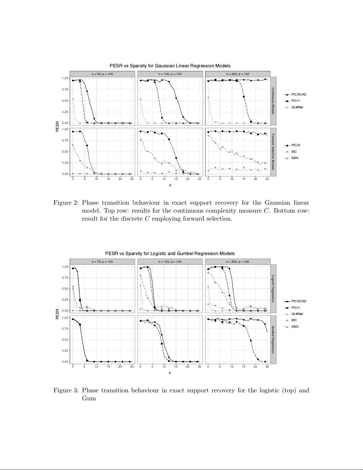
The Piv otal Information Criterion Sylv ain Sardy syl v ain.sardy@unige.ch Maxime v an Cutsem maxime.v ancutsem@unige.ch Dep artment of Mathematics University of Geneva Sara v an de Geer vsara@ethz.ch ETHZ Abstract The Ba yesian and Ak aike information criteria aim at finding a goo d balance b et ween under- and o ver-fitting. They are extensiv ely used every day b y practitioners. Y et we contend they suffer from at least t wo afflictions: their p enalty parameter λ = log n and λ = 2 are to o small, leading to many false disco veries, and their inheren t (b est subset) discrete optimization is infeasible in high dimension. W e alleviate these issues with the pivotal information criterion: PIC is defined as a contin uous optimization problem, and the PIC p enalt y parameter λ is selected at the detection b oundary (under pure noise). PIC’s choice of λ is the quan tile of a statistic that we prov e to b e (asymptotically) pivotal, provided the loss function is appropriately transformed. As a result, simulations sho w a phase transition in the probability of exact support recov ery with PIC, a phenomenon studied with no noise in compressed sensing. Applied on real data, for similar predictive p erformances, PIC selects the least complex mo del among state-of-the-art learners. Keyw ords: Compressed sensing, mo del selection, phase transition, pivotal statistic, sparsit y . 1 In tro duction As computing p ow er and data storage capacity con tinue to increase, along with adv ances in optimization algorithms, researc hers and practitioners allow themselv es to consider highly flexible mo dels with gro wing num b ers of parameters. Suc h flexibility may come at the exp ense of interpretabi lity , parsimony , and sometimes scient ific insight, as predictive per- formance alone b ecomes the primary ob jectiv e. W e are fo cusing on mo del frugality and in terpretability through the use of an information criterion to searc h for a parsimonious mo del and to con trol the ov erfitting without relying on a v alidation set. T o illustrate our ob jectiv e, w e consider the linear regression mo del y = β 0 1 + X β + ϵ , (1) where X is an n × p matrix, β ∈ R p is the parameter v ector of interest, ϵ are errors with v ariance σ 2 , and the in tercept β 0 and σ 2 are n uisance parameters. A well-studied setting is the high-dimensional canonical linear mo del when y i = β i + ϵ i for i = 1 , . . . , n , with n = p (i.e., X = I n ) and Gaussian errors. This simplified mo del has provided imp ortant insigh ts in to parameter estimation. In particular, the James-Stein estimator, a regularized maxi- 1 Sardy, v an Cutsem and v an de Geer m um likelihoo d estimator (James and Stein, 1961), sho wed that the maximum lik eliho o d estimator ˆ β MLE = y is inadmissible when p > 2. As the n umber of predictors grows, assuming β to b e sparse b ecame natural and amounts to assuming only a small p ortion of inputs are b elieved to con tain predictiv e information. The parameter vector β is called sparse if S = { j ∈ { 1 , . . . , p } : β j  = 0 } (2) has a small cardinalit y s := |S | . F or a linear mo del (1), S iden tifies the inputs with predictiv e information, often referred to as ”needles in a ha ystack”. The resulting paradigm centers on detecting these needles, a task closely related to testing. 1.1 Detection b oundary and phase transition Within this sparse paradigm, Donoho and Johnstone (1994) in regression, and Ingster (1997) and Donoho and Jin (2004) in h yp othesis testing, sho wed the existence of a dete ction b ound- ary b elow whic h signal recov ery is hop eless. Sp ecifically , if the nonzero en tries of β are below σ √ 2 r log n , where r ∈ (0 , 1) is a sparsity index, then the nonzero en tries are undetectable, otherwise detection becomes p ossible. This observ ation suggests thresholding observ ations whose magnitude falls b elow φ = σ √ 2 r log n , since attempting to estimate such comp o- nen ts otherwise leads to excessive false disco veries. In particular, in w av elet smo othing, setting the threshold to φ = σ √ 2 log n led to minimax prop erties (Donoho and Johnstone, 1994; Donoho et al., 1995). Ingster et al. (2010) extended the results to high-dimensional regression when the matrix X is no longer the identit y . Observ ed in the testing framework, a phase transition at the detection b oundary has also b een observed in compressed sensing (Donoho, 2006; Cand` es and Romberg, 2007), corresp onding to the noiseless linear mo del y = X β , where X is n × p with p > n and β is assumed s -sparse. F or small sparsity levels and mo derate dimensions, by using the ℓ 1 -minimization estimator min β ∈ R p ∥ β ∥ 1 sub ject to y = X β , exact reco very o ccurs with probabilit y one, but this probabilit y sharply drops to zero as s/p or p/n increases beyond critical thresholds. LASSO (Tibshirani, 1996) extends this approach to noisy settings by solving min β ∈ R p ∥ y − X β ∥ 2 2 + λ ∥ β ∥ 1 , for some regularization parameter λ > 0 chosen to optimize the prediction risk (e.g., via cross-v alidation), although this choice often fails to reco ver the true support S (Su et al., 2015). 1.2 Information criteria The learner w e consider here aims at go o d estimation of β , in particular detection of its nonzero en tries, and is defined as a minimizer of an information criterion (IC). F or a mo del parametrized by β ∈ R p , and an intercept β 0 ∈ R and (p ossibly) a nuisance parameter σ , an IC takes the form IC = L ( β , β 0 , σ ; D ) + λC ( β ) , (3) where D = ( X , y ) ∈ R n × ( p +1) denotes the data, L measures goo dness of fit, and C quantifies mo del complexity . The tuning parameter λ > 0 is fixed a priori (i.e., without v alidation data or cross-v alidation) and lo oks for an ideal compromise b et ween the b eliefs in L and C to select a mo del of appropriate dimension, thereby con trolling under- and ov erfitting. 2 PIC Among information criteria, BIC (Sch warz, 1978) is arguably the most widely used. It emplo ys t wice the negativ e log-lik eliho o d for L and the discrete complexity measure C ( β ) = ∥ β ∥ 0 = # { β j  = 0 , j = 1 , . . . , p } =: s ∈ { 0 , 1 , . . . , p } (4) whic h counts the num b er s of active parameters. F or BIC, the preset v alue is λ = log n , whereas AIC adopts λ = 2 (Ak aike, 1998). Minimizing either criterion yields sparse esti- mators ˆ β , in which some entries are exactly zero, facilitating interpretabilit y by identifying influen tial inputs. The c hoice of λ is crucial: smaller v alues tend to pro duce ov erly complex mo dels that ma y ov erfit and include many false positives, while larger v alues fa vor excessiv e sparsit y . A natural desideratum while minimizing the IC (3) is recov ery of the truly relev ant inputs of the linear mo del (1), that is, matc hing ˆ S = { j ∈ { 1 , . . . , p } : ˆ β j  = 0 } with S in (2). This motiv ates studying the probabilit y of exact supp ort reco very , PESR = P ( ˆ S = S ) , (5) and its phase transition b ehavior as a function of s = |S | , analogous to compressed sensing. This stringen t property is not achiev ed b y classical criteria suc h as BIC or AIC, ev en in ideal conditions such as indep endence of the inputs and high signal-to-noise ratio. Although de- p endence among columns of X further complicates reco very , the indep endent-design setting pro vides an ideal b enchmark for comparing sparse learners. W e use the Gaussian linear regression setting to illustrate limitations of BIC, to which w e discuss our prop osed remedy in Section 2. Assuming Gaussian errors with v ariance σ 2 , BIC = 1 σ 2 RSS s + λs + n log σ 2 with λ = log n, where the b est size- s residual sum of squares are RSS s := min β 0 ∈ R , β ∈ Ω s ∥ y − β 0 1 n − X β ∥ 2 2 with Ω s = { β ∈ R p : ∥ β ∥ 0 = s } . (6) Minimizing ov er s ∈ { 0 , 1 , . . . , min( n, p ) } yields a selected sparsit y lev el ˆ s . AIC replaces λ = log n with λ = 2, leading to a less sparse model when n > exp(2). Regardless of whether one uses BIC, AIC, or some high-dimensional extensions such as Chen and Chen (2008, EBIC) and F an and T ang (2013, GIC), these criteria dep end on the nuisance parameter σ 2 , whose estimation b ecomes c hallenging in high-dimensional settings ( p > n ); see, e.g., F an et al. (2012). Using the maximum likelihoo d estimate ˆ σ 2 , MLE = RSS s /n yields the profile criterion (up to constan ts) BIC = log RSS s n + s log n n . Optimizing ov er s is NP-hard since it requires searc hing o ver all predictor subsets. In practice, one relies on appro ximations suc h as greedy forward selection or the primal–dual activ e set (PD AS) method of Ito and Kunisch (2014). The discrete optimization b ehind BIC is certainly cum b ersome, but the main reason wh y BIC fails to retrieve S stems from the c hoice λ = log n . Sc hw arz (1978) derived this term via a large-sample approximation to the Ba yes factor, whose primary goal is mo del 3 Sardy, v an Cutsem and v an de Geer comparison rather than exact support reco very . Consequen tly , despite its widespread use, BIC is p o orly suited for recov ering S , which in practice leads to sub optimal generalization and in terpretability . Section 3 illustrates this point empirically b y comparing BIC to our prop osed information criterion. 1.3 Our prop osal and pap er organization W e aim at constructing a learner that exhibits a phase transition analogous to compressed sensing, but in the presence of noise. Sp ecifically , when s/p or p/n are small, the learner should recov er S with high probability , while this probability ev entually drops to zero as these ratios increase and the non-zero components of β b ecome undetectable. W e calibrate the learner suc h that, when s = 0, the probability of retrieving S = ∅ is set to 1 − α , for some prescrib ed small α . Starting from a high probabilit y when s = 0 mimics the unit probability prop erty of compressed sensing for small complexity index s ; this pro vides a fa vorable initialization. Our pivotal information criterion (PIC) ac hieves the desirable prop ert y with a pre-sp ecified v alue of λ set at the detection b oundary . The k ey no velt y is the introduction of tw o transformation functions ϕ and g , whic h render the choice of the regularization parameter λ piv otal (i.e., indep endent of unknown parameters). PIC provides a general framework that applies broadly across multiple distributions and accommo dates con tinuous complexity p enalties C ( β ). This paper is organized as follo ws. Section 2 in tro duces the piv otal information crite- rion: Section 2.1 gives its formal definition, Section 2.2 in tro duces the concept of a zero- thresholding function, Section 2.3 explains ho w to mak e the information criterion (asymp- totic) piv otal, Section 2.4 discusses practical implementations and Section 2.5 deriv es the appropriate parameter λ for BIC. Section 3 quantifies the v alidity of the theory and the empirical performance of PIC: Section 3.1 illustrates graphically the piv otality of PIC, Sec- tion 3.2 p erforms Monte-Carlo sim ulations to observe the phase transitions in different settings, and Section 3.3 applies v arious metho ds to six datasets to in vestigate the trade-off b et ween generalization and complexit y . Section 4 finishes with some general commen ts. 2 The piv otal information criterion Man y sparse learners such as Basis Pursuit (Chen et al., 1999), LASSO, or Elastic Net (Zou and Hastie, 2005) rely on con tinuous p enalties, whereas AIC and BIC use a discrete complexit y measure. Ho wev er, what primarily distinguishes an information criterion (3) from a sparse learner is that the regularization parameter λ is pr e-set . Indeed, while learners select λ from the data (e.g., via cross-v alidation), ICs rely on a closed-form mo del-based calibration (e.g., λ = log n for BIC). Two notable learners also use pre-set regularization parameters: wa veshrink c ho oses λ = σ √ 2 log n (Donoho and Johnstone, 1994; Donoho et al., 1995) and square-ro ot LASSO (Belloni et al., 2011) c ho oses λ as a quan tile of a piv otal statistic. The former dep ends on the nuisance parameter σ and is therefore not piv otal, whereas the latter is. 4 PIC 2.1 Definition The pivotal information criterion (PIC) w e prop ose can be seen as a generalization of square- ro ot LASSO b eyond Gaussianity and uses a pre-set v alue for the regularization parameter. Our k ey principle is to c ho ose λ at the detection b oundary , formalized b elow. Definition 1 L et ˆ β λ b e a sp arse le arner indexe d by λ , and let α b e a pr escrib e d smal l pr ob ability. Under H 0 : β = 0 , the value λ α such that P H 0 ( ˆ β λ α = 0 ) = 1 − α is the α -level dete ction b oundary. If λ α do es not dep end on nuisanc e p ar ameters, then we c al l λ PDB α the pivotal dete ction b oundary. Cho osing λ < λ α leads to high false disco v ery rate, whereas λ > λ α unnecessarily compro- mises the c hance of finding the needles. W a veshrink satisfies this prop ert y asymptotically as α → 0 (Donoho and Johnstone, 1994, equation (31)). Since discrete p enalties lead to NP-hard problems, PIC instead relies on a class of con tinuous complexity measures C ℓ 1 to facilitate optimization. Definition 2 L et ρ : R → [0 , ∞ ) b e even and nonde cr e asing on R + . F or β ∈ R p , define C ( β ) = P p i =1 ρ ( β i ) . We say that C ∈ C ℓ 1 is a first-order ℓ 1 -equiv alent complexit y p enalty if lim ϵ → 0 + C ( ϵ β ) ϵ = ∥ β ∥ 1 . This class of measures mo dels complexit y through the magnitude of the co efficients. It includes conv ex pe nalties (e.g., ℓ 1 ) and noncon vex ones such as SCAD (F an and Li, 2001) and MCP (Zhang, 2010) penalties. Although they may differ a wa y from zero, all behav e lik e the ℓ 1 norm to first order near the origin, thereby promoting sparsit y . If one still desires to use BIC’s discrete complexity measure (4), Section 2.5 shows how our metho d still applies to find a go o d λ for BIC. The piv otal information criterion can no w b e defined. Definition 3 Given data D , a b ase loss l n ( θ , σ ; D ) = P n i =1 l ( θ i , σ ; D i ) /n , a c o mplexity me asur e C ∈ C ℓ 1 , p ar ameters β ∈ R p , nuisanc e p ar ameters β 0 ∈ R and σ , and α ∈ (0 , 1) , the Piv otal Information Criterion is PIC = ϕ ( l n ( θ , σ ; D )) + λ PDB α C ( β ) with θ = g ( β 0 1 + X β ) , (7) wher e the pr e-set value of the c omplexity p enalty λ PDB α of Definition 1 is made pivotal thanks to the univariate functions ϕ and g (applie d c omp onentwise), if they exist. By construction, PIC takes the IC form defined in (3) with comp osite loss L = ( ϕ ◦ l n ◦ g ). Finding the functions ( ϕ, g ) is linked to the existence of a zero-thresholding function, whic h w e discuss in Section 2.2. Section 2.3 deriv es ( ϕ, g ) for the location-scale and the one- parameter exp onential families, and Section 2.4 shows ho w to implemen t λ PDB α in practice. Section 2.5 derives λ PDB α for BIC’s nostalgics. 2.2 Zero-thresholding function Consider a sparse learner ˆ β λ defined as the minimizer of the IC defined in (3) with C ∈ C ℓ 1 . Under regularit y conditions, there exists a finite v alue λ 0 > 0 such that ˆ β λ = 0 is a local minimizer of (3) if and only if λ ≥ λ 0 . When the cost function (3) is con vex, this lo cal minim um is also global. The smallest such λ admits a simple characterization, called zero- thresholding function. 5 Sardy, v an Cutsem and v an de Geer Theorem 4 (Zero-thresholding function) L et ˆ β λ minimize (3) and denote τ = ( β 0 , σ ) the nuisanc e p ar ameters. Assume L is twic e differ entiable at ( 0 , ˆ τ ) , wher e ˆ τ satisfies ∇ τ L ( 0 , ˆ τ ; D ) = 0 and the Hessian H L τ ( 0 , ˆ τ ) ≻ 0 . Then the zer o-thr esholding function λ 0 ( L, D ) = ∥∇ β L ( 0 , ˆ τ ; D ) ∥ ∞ (8) satisfies that ( 0 , ˆ τ ) is a lo c al minimizer of (3) if and only if λ ≥ λ 0 ( L, D ) . F or example, the zero-thresholding function of LASSO is λ 0 ( L, D ) = ∥ X T ( y − ¯ y 1 ) ∥ ∞ and that of square-ro ot LASSO is λ 0 ( L, D ) = ∥ X T ( y − ¯ y 1 ) ∥ ∞ / ∥ y − ¯ y 1 ∥ 2 . Giacobino et al. (2017) deriv e the zero-thresholding functions of well-kno wn sparse learners. The α -lev el detection b oundary of Definition 1 can no w b e defined for sparse learners defined as solution to an IC of the form (3). Prop osition 5 Consider the le arner ˆ β λ of The or em 4. L et Y 0 ∼ p τ denote observations gener ate d under the pur e-noise mo del ( β = 0 and τ = ( β 0 , σ ) ). Define the r andom variable Λ = λ 0 ( L, ( X , Y 0 )) and let F Λ denote its cumulative distribution function. Setting λ α = F − 1 Λ (1 − α ) yields P  { ˆ β λ α = 0 is a lo c al minimizer of (3) }  = 1 − α . This is a direct consequence of Theorem 4. The v alue λ α cannot b e computed directly in practice b ecause the statistic Λ may dep end on the unkno wn n uisance parameters τ = ( β 0 , σ ) that generated the data at hand. Moreo ver, real datasets rarely arise from the pure-noise mo del, so reliable estimation of β 0 or σ , esp ecially in high-dimensional settings, is therefore challenging, resulting in p o or calibration of λ α . By rather emplo ying PIC (7), whose transformed loss is L ( β , β 0 , σ ; D ) = ( ϕ ◦ l n ) ( g ( β 0 1 + X β ) , σ ; D ), the law of Λ can b e made asymptotically pivotal through a zero-thresholding function inv olving ϕ ′ and g ′ . Prop osition 6 Consider PIC (7) , wher e ϕ and g ar e strictly incr e asing differ entiable func- tions. Define the sc alar-r estricte d loss ˜ l n ( θ , σ ; D ) := l n ( θ 1 n , σ ; D ) . Assume that under the nul l mo del β = 0 ther e exists ˆ τ = ( ˆ β 0 , ˆ σ ) such that g ( ˆ β 0 ) = ˆ θ MLE and ˆ σ = ˆ σ MLE , and that the sc alar-r estricte d Hessian satisfies ∇ 2 ( θ,σ ) ˜ l n ( ˆ θ MLE , ˆ σ ; D ) ≻ 0 . Then the zer o-thr esholding function of PIC is λ 0 ( ϕ ◦ l n ◦ g , D ) = ϕ ′  ˜ l n  ˆ θ MLE , ˆ σ ; D  · g ′ ( g − 1 ( ˆ θ MLE )) ·    X T ∇ θ l n  ˆ θ MLE 1 , ˆ σ ; D     ∞ . Theorem 4 requires H L τ ( 0 , ˆ τ ) ≻ 0 for the comp osite loss L = ϕ ◦ l n ◦ g . A direct second-order differen tiation with resp ect to ( β 0 , σ ), together with the score equations eliminating first- order terms and the separable c haracter of l n , shows that this condition reduces to p ositive definiteness of the Hessian of ˜ l n at ( ˆ θ MLE , ˆ σ ). The expression for λ 0 then follows from the c hain rule. Notably , λ 0 do es not dep end on the sp ecific p enalt y C , pro vided C ∈ C ℓ 1 . 6 PIC 2.3 Finding ( ϕ, g ) The transformations ( ϕ, g ) pla y a central role in rendering Λ pivotal (Prop osition 5), en- abling calibration of λ at the detection b oundary without accurate estimation of nuisance parameters. The function g transforms the input of the loss l n and is reminiscent of the link function of generalized linear mo dels (Nelder and W edderburn, 1972) and of v ariance stabilizing transformations (Bartlett, 1947). The function ϕ rather transforms the output of the loss. It is imp ortant to observe that ϕ ◦ l n ◦ g employ ed b y PIC is just a comp osite loss function, but b y no means it mo dels the mechanism that generated the data through functions g and ϕ . T ake the Poisson la w for instance, the data can b e generated from a linear mo del with the exp onential canonical link, yet PIC’s composite loss may emplo y a function g  = exp to mak e the c hoice of λ pivotal. Similarly , it is common practice to fit a linear model with the ℓ 2 loss ev en when the data are Poisson. T o find a piv otal pair ( ϕ, g ), we consider loss functions l n of t wo classes of distributions: the location-scale and one-parameter exp onential families. W e let D = ( X , y ) b e the data, where y are realizations from Y 1 , . . . , Y n . Emplo ying the exp onential transformation for ϕ , the following theorem states the finite sample piv otalit y of PIC’s p enalty for the location scale family . Theorem 7 (Lo cation–scale family) Assume f is a fixe d b aseline density such that, c onditional ly on x i , f Y i ( y i | x i ; θ i , σ ) = 1 σ f  y i − θ i σ  , f ( · ) > 0 on R , σ > 0 , wher e θ i = g ( β 0 + x T i β ) . L et l n ( θ , σ ; D ) b e the aver age ne gative lo g-likeliho o d satisfying Pr op osition 6. Then PIC is finite-sample pivotal for ( ϕ, g ) = (exp , id) . W e refer to the resulting estimator as exp onential LASSO . The exp onential transforma- tion implies that exp onen tial LASSO solv es min β ,β 0 ,σ  1 /f Y ( y ; β , β 0 , σ )  1 /n + λ ∥ β ∥ 1 . Profiling ov er σ yields l n ( θ , σ ; D ) ∝ 1 n  P i | y i − θ i | r  1 /r , reco v ering square-root LASSO when r = 2. This means that the r th ro ot is the transformation that makes the r -th loss piv otal, as stated in the follo wing property . Prop ert y 1 F or the Subb otin family (including the Gaussian c ase r = 2 ) with density f Y ( y ; µ, σ ) ∝ σ − 1 exp( −| ( y − µ ) /σ | r ) , the pivotal tr ansformation for the loss l n ( θ , σ ; D ) = 1 n P i | y i − θ i | r is ( ϕ, g ) = ( u 1 /r , id) . Other location–scale distributions than Subb otin include Gumbel and logistic la ws. Asymp- totic conv ergence prop erties of PIC for this family are studied in v an de Geer et al. (2025), and Section 3 illustrates the resulting phase-transition behavior empirically . W e no w consider the one-parameter exp onential family for which, conditionally on x i , log f Y i ( y i | x i ; θ i ) = θ i T ( y i ) − d ( θ i ) + b ( y i ), where the canonical parameter satisfies θ i = g ( β 0 + x T i β ) with g = id. W e develop tw o approac hes. The first one, describ ed in Theorem 7 Sardy, v an Cutsem and v an de Geer 8, uses the classical negative log-lik eliho o d as loss function l n and searches for a pivotal link function g . The second one, described in Theorem 9, in tro duces a new class of losses yielding a weigh ted gradient allowing piv otality , y et k eeping g = id. Condition 1 The ve ctors of variables x 1 , . . . , x n ∈ R p in X ar e fixe d, uniformly b ounde d | x ij | ≤ B n , and standar dize d so that P n i =1 x i = 0 and P n i =1 x 2 ij = n for j = 1 , . . . , p . Condition 2 The numb er of variables p is al lowe d to tend to infinity such that B 4 n (log( pn )) 7 = O ( n 1 − c ) for some c > 0 . Theorem 8 (One-parameter exp onen tial family) L et l n denote the aver age ne gative lo g-likeliho o d optimize d by ˆ β 0 = g − 1 ( ˆ θ MLE ) when β = 0 . Assume ˆ β 0 is c onsistent and β 0 do es not dep end on n , d ∈ C 3 , T ( Y ) has finite fourth moment. Under Conditions 1 and 2, PIC is asymptotic al ly pivotal for ( ϕ, g ) = (id , ˜ d − 1 ) with ˜ d ( θ ) = Z θ p d ′′ ( s ) d s. A close lo ok at the pro of of Theorem 8 sho ws that the first tw o momen ts of Λ are alw ays asymptotically piv otal, but, in particular, Condition 2 on B n is needed for the higher momen ts to b e piv otal as well. This condition implies that X needs to be sufficien tly dense. Example 1 (Bernoulli) In c anonic al form, log f ( y | θ ) = y θ − log (1 + e θ ) with θ = log µ 1 − µ and d ′′ ( θ ) = e θ (1+ e θ ) 2 . So ˜ d ( θ ) = 2 arctan( e θ/ 2 ) (up to a c onstant) and θ i = g ( η i ) = 2 log  tan η i + C 2  , η i = β 0 + x T i β with C is an arbitr ary c entering c onstant. Corr esp ondingly, the Bernoul li p ar ameters ar e µ i = 1 1 + exp  − 2 log(tan η i + C 2 )  = sin 2  η i + C 2  . Cho osing C = π / 2 gives µ (0) = 1 / 2 , le ading to µ i = (sin( η i ) + 1) / 2 for η i ∈ [ − π / 2 , π / 2] , i = 1 , . . . , n . The pivotal reparametrization simplifies the v ariance structure, but it may yield link functions that are monotone only on a restricted in terv al. F or Bernoulli, for example, the parameters need to satisfy linear inequality constrain ts of the form ∥ β 0 + X β ∥ ∞ ≤ π / 2. This induces constrained optimization in ( β 0 , β ), whic h is undesirable for computation. This motiv ates the second approac h. Theorem 9 (W eigh ted score loss) Under the same assumptions as The or em 8, PIC is asymptotic al ly pivotal for ( ϕ, g ) = (id , id) when c onsidering the loss function l n ( θ , D ) = 1 n n X i =1 Z θ i d ′ ( s ) − T ( y i ) p d ′′ ( s ) d s. 8 PIC If one is interested in using another link function g  = id, the pro of of Theorem 9 deriv es the corresponding weigh ted loss. Example 2 (Bernoulli) Basic inte gr ation le ads to the loss l n ( θ , D ) = 1 n P n i =1 2 y i e − θ i / 2 + 2(1 − y i ) e θ i / 2 with θ i = β 0 + x T i β , or, with µ i = 1 / (1 + e − θ i ) , 1 n n X i =1 2 y i r 1 − µ i µ i + 2(1 − y i ) r µ i 1 − µ i . Example 3 (P oisson) In c anonic al form, log f ( y | θ ) = y θ − exp( θ ) with θ = log( µ ) and d ′ ( θ ) = d ′′ ( θ ) = exp( θ ) . The c orr esp onding weighte d loss is l n ( θ , D ) = 1 n P n i =1 2 y i e − θ i / 2 + 2 e θ i / 2 with θ i = β 0 + x T i β , or, with µ i = exp( θ i ) , 1 n n X i =1 2 y i √ µ i + 2 √ µ i . T able 1 summarizes common instances and rep orts the corresp onding gradient expres- sions ∇ entering the zero-thresholding statistic Λ = ∥∇∥ ∞ . F or the one-parameter exp o- nen tial family , the link g and loss are expressed for the natural distribution parameter µ . W e also list tw o transformations for the Laplace case and Co x’s surviv al analysis. 2.4 The piv otal detection b oundary λ PDB α in practice The piv otal detection b oundary λ PDB α is defined as the (1 − α )-quantile of the random v ari- able Λ in Proposition 5. By construction for the prescrib ed pairs ( ϕ, g ), the random v ariable Λ is pivotal for the location–scale family and asymptotically pivotal for the one-parameter exp onen tial family , so its (asymptotic) distribution does not depend on the n uisance param- eters τ = ( β 0 , σ ). Hence, a natural approach to ev aluate λ PDB α is Monte Carlo sim ulation. Sp ecifically , one generates M resp onse vectors y ( m ) 0 , m = 1 , . . . , M , under the n ull mo del Y 0 ∼ p τ for any c hosen nuisance parameters τ , compute λ ( m ) = ∥∇ ( m ) ∥ ∞ , and tak e the empirical (1 − α )-quantile of λ (1) , . . . , λ ( M ) . Increasing M yields an arbitrarily accurate finite-sample appro ximation of λ PDB α . Despite its conceptual app eal and highly parallelizable nature, the Mon te Carlo calibra- tion ma y b ecome computationally demanding in practice. This is esp ecially true in large sample settings or settings where the ev aluation of the gradien t requires rep eated maximum lik eliho o d computations without closed form (e.g., Gumbel). This motiv ates the follo wing result that bypasses explicit sim ulations of Y 0 . Prop osition 10 (Asymptotic Gaussian calibration) Under Conditions 1 and 2, let ˆ Σ X = 1 n P n i =1 x i x T i denote the (normalize d) Gr am matrix. F or the mo dels given in T able 1 with their c orr esp onding tr ansformations ( ϕ, g ) and c onstant c , an asymptotic appr oximation is F − 1 Λ (1 − α ) ≈ q 1 − α  1 √ n    N (0 , c ˆ Σ X )    ∞  , wher e q 1 − α denotes the (1 − α ) -quantile. 9 Sardy, v an Cutsem and v an de Geer La w Loss l n g ( u ) Dom( g ) ϕ ( v ) ∇ c L o c ation-sc ale family Gaussian NLL u R exp v q 2 π e n X T ( y − ¯ y1 ) ∥ y − ¯ y1 ∥ 2 2 π e Gaussian MSE u R √ v X T ( y − ¯ y1 ) / √ n ∥ y − ¯ y1 ∥ 2 1 Gum b el NLL u R exp v e 1+ ¯ z n X T ( e z − 1 ) ( ∗ ) e 2( γ +1) Subb otin ( r > 1) M r th E u R v 1 /r r 2 − 2 /r Γ(2 − 1 /r ) Γ(1 /r ) Laplace ( r = 1) MAE u R v X T sign( y − y m 1 ) /n † 1 One-p ar ameter exp onential family Bernoulli NLL 1+sin u 2 [ − π 2 , π 2 ] v X T ( y − ¯ y1 ) /n √ ¯ y (1 − ¯ y ) 1 Bernoulli WSL 1 1+ e − u R v X T ( y − ¯ y1 ) /n √ ¯ y (1 − ¯ y ) 1 P oisson NLL u 2 4 R + v X T ( y − ¯ y1 ) /n √ ¯ y 1 P oisson WSL exp u R v X T ( y − ¯ y1 ) /n √ ¯ y 1 Exp onen tial NLL exp u R v X T ( y − ¯ y1 ) /n ¯ y 1 Survival analysis Co x mo del NLPL u R √ v ( § ) 1 4 log n T able 1: Examples of transformation pairs ( g , ϕ ) for constructing PIC. The notation ’NLL’ is for the negative log-lik eliho o d, ’WSL’ is for the weigh ted score loss, MSE for the mean squared error and MAE for the mean absolute error. F or the one-parameter exp onen tial family , g maps the natural distribution parameter. ( ∗ ) z = ( y − ˆ µ 1 n ) / ˆ σ and ¯ z = ( ¯ y − ˆ µ ) / ˆ σ , where ˆ µ and ˆ σ are the MLEs; ( † ) y m is the median (Sardy et al., 2025); ( § ) ’NLPL’ is Co x’s negative log-partial lik eliho o d (v an Cutsem and Sardy, 2025). 10 PIC This result is prov en for the one-parameter exp onential family in Theorem 8 and follows from v an de Geer et al. (2025) for the lo cation-scale family . This asymptotic c alibr ation reduces the problem to simulating Gaussian vectors with co v ariance ˆ Σ X , thereby a v oiding rep eated MLE computations. A further simplification neglects correlations among regressors b y replacing ˆ Σ X b y the iden tit y matrix: q 1 − α  1 √ n ∥N (0 , I p ) ∥ ∞  ≈ 1 √ n Φ − 1  1 − α 2 p  ≈ s 2 n log  2 p α  . This yields a simple closed-form rule for PIC’s pre-set λ , alb eit slightly conserv ativ e. 2.5 Giving BIC a second c hance Section 1.2 sho wed that the Bay esian Information Criterion (BIC) has a lo w probabilit y of exact support reco very in moderate to high dimension. T o fix BIC, we simply need to d erive the zero-thresholding function of the discrete complexity measure (4) for an appropriate ( ϕ, g )-transformation suc h that the corresp onding statistic Λ is piv otal. As it turns out, the follo wing theorem states that, with no transformation, BIC is already piv otal so that λ can b e selected at the piv otal detection b oundary . Theorem 11 (Piv otal BIC) Consider the discr ete me asur e of c omplexity C define d in (4) and let l n ( θ , σ ; D ) b e twic e the ne gative lo g-likeliho o d of the Gaussian law employe d by BIC. Then, with the identity tr ansformations ( g , ϕ ) = (id , id) , the zer o-thr esholding function is λ 0 ( L, D ) = max s =1 ,..., min( p,n − 2) 1 s log  RSS 0 RSS s  (9) with RSS s define d in (6) , and the r esulting IC is finite sample pivotal. Theorem 11 shows that BIC can b e em b edded within the PIC framework by calibrat- ing its penalty at the detection edge. In practice, how ever, computing the BIC’s zero- thresholding function (9) is infeasible in high dimension, as it requires solving an NP-hard optimization problem. This dra wback highligh ts another adv antage of using PIC’s con- tin uous p enalty . A natural compromise for BIC is to replace b est subset selection by a discrete notion of local minimalit y . F or (one step) forw ard selection, the corresp onding zero-thresholding function reduces to λ 0 ( L, D ) = log( RSS 0 RSS 1 ). 3 Sim ulation studies 3.1 Illustration of (non-)piv otal transformations Figure 1 illustrates the pivotal detection boundary mechanism induced by a suitable pair ( ϕ, g ) in the canonical P oisson mo del ( X = I n ) with unknown background in tensity θ 0 . Since X = I n , the m ultiv ariate loss decomp oses into n independent univ ariate losses, and the comp onents of the gradient ∇ β ( ϕ ◦ l n ◦ g )( 0 , ˆ β 0 ; D ) provide the information needed to distinguish signals from noise. The top row shows three sim ulated datasets ( n = 500) with background mean µ 0 ∈ { 36 , 4 , 144 } and sparsity lev els s ∈ { 0 , 3 , 3 } , where the nonzero coefficients scale prop ortion- ally with µ 0 . The second ro w displays the comp onent wise magnitude   ∇ β ( ϕ ◦ l n ◦ g )( 0 , ˆ β 0 ; D )   , 11 Sardy, v an Cutsem and v an de Geer 0 100 200 300 0.00 0.01 0.02 0.03 0 100 200 300 400 500 0.0 0.1 0.2 0.3 0 100 200 300 400 500 0 100 200 300 400 500 x value std: 6.0 std: 2.0 std: 12.0 Response (y) Pivotal gradient Non-pivotal gradient Figure 1: Illustration of the detection boundary induced by PIC’s composite loss in the canonical P oisson mo del ( X = I n ). T op ro w: sim ulated datasets with v arying bac kground intensities and sparsity levels s ∈ { 0 , 3 , 3 } . Middle row: comp onent- wise magnitude of the pivotal gradien t. Bottom row: corresp onding analysis for the non pivotal gradient of the canonical GLM c hoice. obtained using PIC’s pivotal pair ( ϕ, g ) = (id , u 2 4 ) for the av erage negative log-lik eliho o d l n . The red line indicates λ PDB α , the α -upp er quantile of Λ with α = 0 . 05. By construc- tion, the resulting detection b oundary is inv ariant across the null h yp othesis H 0 (left panel) and the alternative scenarios H 1 (middle and right panels) and cleanly separates the signal comp onen ts from the bac kground noise. Under the null ( s = 0), the piv otal calibration cor- rectly thresholds all coefficients to zero, while under the alternativ es ( s = 3) it successfully iden tifies the true signals and suppresses spurious fluctuations. In con trast, the third row shows the analysis p erformed with the canonical GLM choice ( ϕ, g ) = (id , exp). Here the detection b oundary dep ends on the data through n uisance parameter estimation and therefore v aries across panels. But when these n uisance parame- ters are po orly estimated (ov erestimated on bottom middle plot and underestimated on the b ottom righ t plot), the resulting threshold fails to reliably distinguish signals from noise. 3.2 Empirical Phase T ransition Analysis W e ev aluate the p erformance of the prop osed metho ds through an empirical phase tran- sition analysis in the probabilit y of exact supp ort recov ery (PESR) as a function of the sparsit y level s . The study cov ers three regression settings: Gaussian, logistic, and Gum b el regression. W e compare our approac hes against three established baselines: BIC, EBIC, 12 PIC and GLMNet. The first tw o p erform v ariable selection by minimizing BIC( s ) = − 2 log L n ( ˆ β 0 , ˆ β s ) + s log n, EBIC γ ( s ) = − 2 log L n ( ˆ β 0 , ˆ β s ) + s log n + 2 γ log  p s  , where L n denotes the likelihoo d function and γ = 0 . 5. Both BIC and EBIC are imple- men ted via forw ard selection. The third baseline uses the glmnet pack age in R to compute the LASSO estimator with the regularization parameter c hosen b y 10-fold cross-v alidation minimizing the empirical loss. F or eac h sparsity lev el s , w e generate m = 200 indep enden t datasets. The linear predic- tor is defined as η ( s ) i = β 0 + x ⊤ i β s for i = 1 , . . . , n , where β 0 = 0, x i ∈ R p has indep enden t standard Gaussian entries, and β s ∈ R p con tains exactly s non-zero co efficients, each set to 3. The supp ort of β s is selected uniformly at random for eac h dataset. The resp onse v ariables y ( s ) i are generated conditionally on η ( s ) i . F or the Gaussian case, y ( s ) i = η ( s ) i + ϵ i with ϵ i dra wn from standard Gaussians. W e fix p = 100 and consider n ∈ { 50 , 100 , 200 } in order to explore regimes ranging from high-dimensional ( n < p ) to o v erdetermined ( n > p ). Both PIC:SCAD and PIC: ℓ 1 are constructed according to (3), with l n the mean squared error loss with the appropriate transformations ϕ = √ · and g = id, as sp ecified in T able 1. The regularization parameter is selected as λ PDB α with α = 0 . 05. The PIC:SCAD v ariant uses the SCAD p enalty with parameter a = 3 . 7 (default v alue). PIC: ℓ 0 follo ws the prop osed pro cedure describ ed in Section 2.5. Figure 2 presents the results. Among the compared pro cedures, our meth- o ds are the only ones that exhibit a sharp phase transition. In particular, the transition b et ween near-perfect recov ery and systematic failure is clearly visible, and shifts with in- creasing n . Among the baselines, EBIC consistently outp erforms BIC, esp ecially in the high-dimensional regime. BIC p erforms reasonably only when n ≫ p , where the classi- cal asymptotic justification b ecomes more appropriate. GLMNet p erforms worst ov erall in terms of exact supp ort recov ery , typically failing to displa y a clear phase transition and sho wing substan tially lo wer PESR v alues across sparsit y lev els. In the logistic regression setting, the resp onses are generated as y ( s ) i ∼ Bernoulli( σ ( η ( s ) i )) where σ ( t ) = 1 / (1 + e − t ) denotes the logistic function. In this case, b oth PIC:SCAD and PIC: ℓ 1 are implemented using the weigh ted score loss introduced in Theorem 9, together with the corresponding transformations sp ecified in T able 1. The results for p = 100 and n ∈ { 75 , 150 , 300 } are display ed in Figure 3. The b ehavior mirrors that of the Gaussian setting: our metho ds display a clear phase transition, whereas the baselines show a more gradual degradation in p erformance. Compared to the Gaussian setting, the logistic case highligh ts the increased difficulty of binary classification for exact support recov ery . F or the Gum b el regression setting, y ( s ) i = η ( s ) i + ϵ i with ϵ i dra wn from Gumbel(0 , 2). Figure 3 presents the corresp onding phase transition results. Here, baseline comparisons are not included, as neither glmnet nor statsmodels (used for the forward-selection-based comp etitors) pro vides direct support for this mo del. Consequen tly , the analysis fo cuses on the proposed PIC-based methods, which again exhibit a clear phase transition. 13 Sardy, v an Cutsem and v an de Geer 0.00 0.25 0.50 0.75 1.00 0 5 10 15 20 25 0.00 0.25 0.50 0.75 1.00 0 5 10 15 20 25 0 5 10 15 20 25 PESR vs Sparsity for Gaussian Linear Regression Models s PESR n = 50, p = 100 n = 100, p = 100 n = 200, p = 100 Continuous Models Forward Selection Models PIC:SCAD PIC:l1 GLMNet PIC:l0 BIC EBIC Figure 2: Phase transition b ehaviour in exact supp ort recov ery for the Gaussian linear mo del. T op row: results for the contin uous complexit y measure C . Bottom ro w: result for the discrete C employing forward selection. 0.00 0.25 0.50 0.75 1.00 0 5 10 15 20 25 0.00 0.25 0.50 0.75 1.00 0 5 10 15 20 25 0 5 10 15 20 25 PESR vs Sparsity for Logistic and Gumbel Regression Models s PESR n = 75, p = 100 n = 150, p = 100 n = 300, p = 100 Logistic Regression Gumbel Regression PIC:SCAD PIC:l1 GLMNet BIC EBIC Figure 3: Phase transition b ehaviour in exact supp ort recov ery for the logistic (top) and Gum b el (b ottom) regression mo del. 14 PIC 3.3 Real data exp eriments W e no w complemen t the syn thetic phase transition analysis with an empirical study on real- w orld datasets, fo cusing on b oth v ariable selection b eha vior and predictiv e p erformance. In particular, we consider six datasets: three corresponding to Gaussian regression tasks and three corresp onding to binary classification problems. F or eac h dataset, categorical v ariables are enco ded using dumm y v ariables when applicable, and missing v alues are handled via simple imputation using either the mean (for n umerical v ariables) or the most frequent category (for categorical v ariables). All cov ariates are standardized before training. T able 2 summarizes the main c haracteristics of eac h dataset after prepro cessing. Dataset Source n p Regression datasets Prostate Cancer Kaggle 97 8 Comm unities & Crime UCI 1994 100 Rib ofla vin R: hdi 71 4088 Binary classification datasets Breast Cancer scikit-learn 569 30 Ionosphere UCI 351 33 Sonar UCI 208 60 T able 2: Considered datasets with some key c haracteristics. F or eac h dataset, we perform 100 indep enden t random train-test splits, where the test set represents 30% of the total observ ations and the remaining 70% is used for training. All mo del fitting and v ariable selection procedures are carried out exclusively on the training data, after which predictive p erformance is ev aluated on the test set. Performance metrics are c hosen according to the task: mean squared error is used for regression tasks, whereas classification accuracy is used for binary classification. F ollowing v ariable selection, all metho ds are refitted without regularization on the selected features prior to ev aluation. T able 3 summarizes the results. Ov erall, the conclusions are consistent with those observ ed in the previous section. The cross-v alidated GLMNet approac h achiev es strong predictiv e p erformance but tends to retain a relativ ely large n umber of features, resulting in less parsimonious mo dels. In con trast, the information criterion-based approaches, particu- larly EBIC, consisten tly select substantially smaller subsets of v ariables while main taining comp etitiv e predictive accuracy . How ever, for similar levels of predictive accuracy , the PIC pro cedures ac hieve greater parsimon y by selecting few er v ariables. According to Occam’s razor this makes the PIC approac hes particularly app ealing in practice. 4 Conclusions and future w ork BIC has b een known to underp enalize complexity , causing false detections in many data analyses. A ttempts to alleviate this problem ha ve b een to increase BIC’s p enalt y (e.g., EBIC and GIC) or to mo dify cross-v alidation with the one standard error rule (Breiman 15 Sardy, v an Cutsem and v an de Geer Dataset PIC:SCAD PIC: ℓ 1 PIC: ℓ 0 GLMNet BIC EBIC Regression Prostate Cancer 0 . 60 2 . 7 ± 0 . 1 0 . 58 3 . 2 ± 0 . 1 0 . 64 2 . 2 ± 0 . 1 0 . 59 5 . 8 ± 0 . 2 0 . 59 3 . 0 ± 0 . 1 0 . 60 2 . 9 ± 0 . 1 Comm unities & Crime 0 . 02 12 . 5 ± 0 . 2 0 . 02 12 . 5 ± 0 . 2 0 . 02 9 . 0 ± 0 . 2 0 . 02 58 . 3 ± 2 . 2 0 . 02 11 . 6 ± 0 . 3 0 . 02 10 . 7 ± 0 . 2 Rib ofla vin 0 . 35 6 . 1 ± 0 . 2 0 . 36 6 . 1 ± 0 . 2 0 . 53 2 . 4 ± 0 . 1 0 . 48 35 . 5 ± 1 . 4 0 . 67 48 . 8 ± 0 . 1 0 . 46 8 . 7 ± 1 . 2 Classification Breast Cancer 0 . 96 3 . 5 ± 0 . 1 0 . 96 4 . 2 ± 0 . 1 – 0 . 96 13 . 0 ± 0 . 3 0 . 96 5 . 6 ± 0 . 3 0 . 96 5 . 0 ± 0 . 2 Ionosphere 0 . 87 4 . 3 ± 0 . 1 0 . 87 4 . 6 ± 0 . 1 – 0 . 88 16 . 6 ± 0 . 4 0 . 87 11 . 3 ± 0 . 5 0 . 87 8 . 9 ± 0 . 3 Sonar 0 . 71 3 . 0 ± 0 . 2 0 . 71 3 . 8 ± 0 . 2 – 0 . 73 20 . 1 ± 0 . 6 0 . 73 13 . 8 ± 0 . 6 0 . 72 7 . 1 ± 0 . 5 T able 3: Comparison of PIC-based metho ds with GLMNet, BIC, and EBIC on standard regression and classification b enchmarks. The first line in each en try reports the mean predictive performance. F or regression tasks, p erformance is measured b y predictiv e error (low er is b etter), whereas for classification tasks p erformance is measured b y accuracy (higher is b etter). The second line in eac h entry rep orts the a verage mo del size (mean ± standard deviation) ov er repeated data splits. et al., 1984). These metho ds seem ad ho c and ha ve not b een designed to induce a phase transition. In empirical studies, these metho ds tend to select too many cov ariates. The prop osed metho d defines a new general framework to balance generalization and complexit y in a wa y that mimics the phase transition achiev ed by compressed sensing. The probabilistic selection of λ is calibrated to con trol the false disco very rate under the n ull mo del. PIC generalizes square-ro ot LASSO to the lo cation-scale and one-parameter expo- nen tial families, and can b e naturally extended further b eyond linear models and b eyond regression or classification tasks; v an Cutsem and Sardy (2025) apply PIC to surviv al analy- sis. The piv otality prop erty of the gradient could also b e emplo yed further in gradien t-based regularization. 16 PIC App endix A. Pro of of Theorem 4 Let f ( β , τ ) = L ( β , τ ) + λC ( β ) with C ∈ C ℓ 1 . Denote ζ = ( β , τ ), ζ 0 = ( 0 , ˆ τ ), where ˆ τ minimizes L at β = 0 . Let ζ ϵ = ζ 0 + ϵ h with h = ( d β , d τ ). A second-order T a ylor expansion of L around ζ 0 , com bined with the first-order optimalit y conditions in τ , yields L ( ζ ϵ ) = L ( ζ 0 ) + ϵd T β ∇ β L ( ζ 0 ) + ϵ 2 2 h T H ζ ( ζ 0 ) h + o ( ϵ 2 ) . Since C ∈ C l , f ( ζ ϵ ) − f ( ζ 0 ) = ϵd T β ∇ β L ( ζ 0 ) + ϵ 2 2 h T H ζ ( ζ 0 ) h + λ | ϵ |∥ d β ∥ 1 + o ( ϵ 2 ) . By H¨ older’s inequality , | d T β ∇ β L ( ζ 0 ) | ≤ ∥∇ β L ( ζ 0 ) ∥ ∞ · ∥ d β ∥ 1 , whic h implies f ( ζ ϵ ) − f ( ζ 0 ) ≥ | ϵ |  λ − ∥∇ β L ( ζ 0 ) ∥ ∞  ∥ d β ∥ 1 + ϵ 2 2 h T H ζ ( ζ 0 ) h + o ( ϵ 2 ) . W riting h T H ζ ( ζ 0 ) h = d T β H β β d β + 2 d T β H β τ d τ + d T τ H τ τ d τ , w e distinguish directions with d β = 0 , for which p ositivit y follows from H τ τ ( ζ 0 ) ≻ 0, and directions with d β  = 0 , where the linear p enalty term dominates all quadratic con tributions for sufficien tly small ϵ . Hence ζ 0 is a lo cal minimizer of f if and only if λ > ∥∇ β L ( ζ 0 ) ∥ ∞ , yielding the stated zero-thresholding function. App endix B. Pro of of Theorem 7 F or the lo cation-scale family , the negative log-likelihoo d is l n ( θ , σ ; D ) = log σ − 1 /n P n i =1 log f (( y i − θ ) /σ ). So with ϕ = exp, the zero-thresholding function is λ 0 (exp( l n ) , D ) = exp log ˆ σ MLE − 1 n n X i =1 log f ( y i − ˆ θ MLE ˆ σ MLE ) ! ·      X T 1 n ˆ σ MLE n X i =1 f ′ (( y i − ˆ θ MLE ) / ˆ σ MLE ) f (( y i − ˆ θ MLE ) / ˆ σ MLE )      ∞ = 1 n exp − 1 n n X i =1 log f ( y i − ˆ θ MLE ˆ σ MLE ) ! ·      X T n X i =1 f ′ (( y i − ˆ θ MLE ) / ˆ σ MLE ) f (( y i − ˆ θ MLE ) / ˆ σ MLE )      ∞ . Supp ose D ′ = ( X , y ′ ) with y ′ = a y + b with a > 0, then, b y definition of the lo cation scale family , y ′ is a sample from the same law as y but with parameters ( θ ′ , σ ′ ). Moreov er, since an affine transform is monotone, we ha ve that ˆ θ ′ MLE = a ˆ θ MLE + b and ˆ σ ′ MLE = a ˆ σ MLE . So λ 0 (exp ◦ l n , D ′ ) = λ 0 (exp ◦ l n , D ), pro ving that PIC is piv otal for the lo cation-scale family . 17 Sardy, v an Cutsem and v an de Geer App endix C. Pro of of Theorem 8 and 9 Assuming a one-parameter exp onen tial family in canonical form log f ( y i | θ i ) = θ i T ( y i ) − d ( θ i ) + b ( y i ), and a link θ i = g ( η i ) for η i = β 0 + x T i β leads to the negativ e log-lik eliho o d l n ( θ , D ) = 1 n n X i =1 d ′ ( θ i ) − T ( y i ) . T o create piv otality , we rather consider a general class of loss functions of the form l n ( θ , D ) = 1 n n X i =1 A ( θ i ) − w ( θ i ) T ( y i ) , where w is a differen tiable function. Imp osing A ′ ( θ ) = d ′ ( θ ) w ′ ( θ ) ensures Fisher consistency . Note that choosing w ( θ ) = θ reco vers the negativ e log-lik eliho o d. The considered loss allo ws for a weigh ted gradient H := { h β 0 ( y i , x i ) =  T ( y i ) − d ′ ( g ( β 0 ))  w ′ ( g ( β 0 )) g ′ ( β 0 ) x i , β 0 ∈ C } , where h β 0 ( y i , x i ) denotes the one-sample gradient with res pect to β ev aluated at β = 0 , and C is a compact set. The zero-thresholding function (8) of l n is ∥ 1 n P n i =1 h ˆ β 0 ( y i , x i ) ∥ ∞ =: ∥ P n h ˆ β 0 ∥ ∞ . Thanks to the centering assumption P i x i = 0 , P n h ˆ β 0 = 1 n n X i =1 h ˆ β 0 ( y i , x i ) = 1 n n X i =1  T ( y i ) − d ′ ( g ( t ))  w ′ ( g ( ˆ β 0 )) g ′ ( ˆ β 0 ) x i , for all t , in particular for the true parameter v alue t = β 0 . Therefore √ n  P n h ˆ β 0 − P n h β 0  = √ n  w ′ ( g ( ˆ β 0 )) g ′ ( ˆ β 0 ) − w ′ ( g ( β 0 )) g ′ ( β 0 )  · 1 n n X i =1  T ( y i ) − d ′ ( g ( β 0 ))  x i . Assuming the map t 7→ w ( g ( t )) is t wice differen tiable at β 0 , b y consistency and the Delta metho d, the first term is of order O P (1). Moreov er, the second term is of the form 1 n X T ϵ , where ϵ i = T ( y i ) − d ′ ( g ( β 0 )) has mean zero and is sub-exp onential. Using Ho effding and union bounds, the second term is of order o P (1). Hence,    √ n  P n h ˆ β 0 − P n h β 0     ∞ = O P (1) · o P (1) = o P (1) . So ∥ √ nP n h ˆ β 0 ∥ ∞ = ∥ √ nP n h β 0 ∥ ∞ + o P (1) . Define v i = h β 0 ( y i , x i ) = ( T ( y i ) − d ′ ( g ( β 0 ))) w ′ ( g ( β 0 )) g ′ ( β 0 ) x i = ξ i x i , so that ∥ √ nP n h β 0 ∥ ∞ = ∥ 1 √ n P i v i ∥ ∞ . Note that v i are indep endent v ectors and v ij = x ij ξ i with E [ ξ i ] = 0 and E [ ξ 2 i ] = ( w ′ ( g ( β 0 )) g ′ ( β 0 )) 2 d ′′ ( g ( β 0 )). Hence, imp osing w ′ ( g ( t )) g ′ ( t ) = 1 p d ′′ ( g ( t )) , 18 PIC implies a cov ariance free of the nuisance parameter. Cho osing w ( θ ) = θ determines the piv otal link g of Theorem 8, whereas fixing the canonical link θ = g ( η ) = η leads to the loss of Theorem 9. F urther assuming E [ ξ 4 i ] < ∞ , Chernozh uko v et al. (2013) show ed that, under the as- sumptions of the theorem, sup t ∈ R      P  ∥ √ nP n h β 0 ∥ ∞ ≤ t  − P ( ∥ 1 √ n n X i =1 z i ∥ ∞ ≤ t )      → 0 , where z 1 , . . . , z n are independent centered Gaussian random vectors in R p suc h that eac h z i and t i share the same co v ariance matrix. Consequently , for an y fixed α ∈ (0 , 1), the (1 − α )-quantile of ∥ √ nP n h β 0 ∥ ∞ can b e consisten tly appro ximated b y the (1 − α )-quantile of ∥ N (0 , Σ X ) ∥ ∞ with Σ X = 1 n P n i =1 x i x T i . App endix D. Pro of of Theorem 11 Twice the negative log-likelihoo d com bined with the prop osed transformations yields L ( β , β 0 , σ ; D ) = 1 σ 2 ∥ y − β 0 1 n − X β ∥ 2 2 n + log(2 π σ 2 ) . Let RSS s b e the b est size s residuals some of squares defined in (6). F or fixed s , w e ha ve that ( ˆ σ MLE ) 2 = RSS s /n , so the profile information criterion is IC = 1 + log(2 π RSS s /n ) + λs . T o ensure s = 0 is a minimizer of the IC, λ m ust b e large enough so that 1 + log(2 π RSS 0 /n ) ≤ 1 + log(2 π RSS s /n ) + λs, for all s ≥ 1 . Therefore the zero-thresholding function is that giv en in (9). So the statistic Λ = λ 0 ( L, ( X , Y 0 )) is piv otal with resp ect to ( β 0 , σ ) since RSS s /σ 2 is piv otal for all s . References H. Ak aik e. Information theory and an extension of the maxim um lik eliho o d principle. In Sele cte d Pap ers of Hir otugu Akaike , pages 199–213. Springer, 1998. M. S. Bartlett. The Use of Transformations. Biometrics , 3(1):39–52, 1947. A. Belloni, V. Chernozh uk ov, and L. W ang. Square-ro ot lasso: piv otal reco very of sparse signals via conic programming. Biometrika , 98(4):791–806, 2011. L. Breiman, J. F riedman, R. Olshen, and C. Stone. Classific ation and R e gr ession T r e es . Routledge, Boca Raton, 1984. E. Cand` es and J. Romberg. Sparsity and incoherence in compressive sampling. Inverse Pr oblems , 23(3):969–985, 2007. J. Chen and Z. Chen. Extended Ba y esian information criteria for mo del selection with large mo del spaces. Biometrika , 95(3):759–771, 2008. 19 Sardy, v an Cutsem and v an de Geer S. S. Chen, D. L. Donoho, and M. A. Saunders. A tomic decomp osition by basis pursuit. SIAM Journal on Scientific Computing , 20(1):33–61, 1999. V. Chernozh uko v, D. Chetv eriko v, and K. Kato. Gaussian approximations and m ultiplier b o otstrap for maxima of sums of high-dimensional random vectors. The Annals of Statis- tics , 41(6), December 2013. D. Donoho and J. Jin. Higher criticism for detection sparse heterogeneous mixtures. Annals of Statistics , 32:962–994, 2004. D. L. Donoho. Compressed sensing. IEEE T r ansactions on Information The ory , 52:1289– 1306, 2006. D. L. Donoho and I. M. Johnstone. Ideal spatial adaptation b y wa velet shrink age. Biometrika , 81(3):425–455, 1994. D. L. Donoho, I. M. Johnstone, G. Kerkyac harian, and D. Picard. W a v elet shrink age: asymptopia? Journal of the R oyal Statistic al So ciety: Series B , 57(2):301–369, 1995. J. F an and R. Li. V ariable selection via nonconca ve p enalized lik eliho o d and its oracle prop erties. Journal of the Americ an Statistic al Asso ciation , 96(456):1348–1360, 2001. J. F an, S. Guo, and N. Hao. V ariance estimation using refitted cross-v alidation in ultrahigh dimensional regression. Journal of the R oyal Statistic al So ciety: Series B , 74(1):37–65, 2012. Y. F an and C. Y. T ang. T uning parameter selection in high dimensional penalized lik eliho o d. Journal of the R oyal Statistic al So ciety: Series B , 75(3):531–552, 2013. C. Giacobino, S. Sardy , J. Diaz-Rodriguez, and N. Hengartner. Quan tile universal threshold. Ele ctr on. J. Statist. , 11(2):4701–4722, 2017. Y. I. Ingster. Some problems of h yp othesis testing leading to infinitely divisible distribution. Mathematic al Metho ds of Statistics , 6:47–69, 1997. Y. I. Ingster, A. B. Tsybak ov, and N. V erzelen. Detection b oundary in sparse regression. Ele ctr onic Journal of Statistics , 4:1476–1526, 2010. K. Ito and K. Kunisch. A v ariational approach to sparsit y optimization based on Lagrange m ultiplier theory. Inverse Pr oblems , 30(1), 2014. W. James and C. Stein. Estimation with quadratic loss. In Pr o c e e dings of the F ourth Berkeley Symp osium on Mathematic al Statistics and Pr ob ability, V olume 1: Contribu- tions to the The ory of Statistics , pages 361–379, Berkeley , California, 1961. Univ ersity of California Press. J. A. Nelder and R. W. M. W edderburn. Generalized linear mo dels. Journal of the R oyal Statistic al So ciety: Series A , 135(3):370–384, 1972. S. Sardy , I. Mizera, Xiaoyu Ma, and H. Gaible. The ∞ -s test via regression quan tile affine LASSO. ArXiv , arXiv:2409.04256, 2025. 20 PIC G. Sc h warz. Estimating the dimension of a mo del. The A nnals of Statistics , 6(2):461–464, 1978. W. Su, M. Bogdan, and E. Candes. F alse discov eries o ccur early on the lasso path. The A nnals of Statistics , 45:2133–2150, 11 2015. R. Tibshirani. Regression shrink age and selection via the lasso. Journal of the R oyal Statistic al So ciety, Series B , 58(1):267–288, 1996. M. v an Cutsem and S. Sardy . Square ro ot co x’s surviv al analysis b y the fittest linear and neural net w orks mo del. ArXiv , arXiv:2510.19374, 2025. S. v an de Geer, S. Sardy , and M. v an Cutsem. A piv otal transform for the high-dimensional lo cation-scale model. A rXiv , abs/2109.06098, 2025. C.-H. Zhang. Nearly unbiased v ariable selection under minimax concav e p enalty . The A nnals of Statistics , 38(2), 2010. H. Zou and T. Hastie. Regularization and v ariable selection via the elastic net. Journal of the R oyal Statistic al So ciety: Series B , 67(2):301–320, 2005. 21