Clipped Gradient Methods for Nonsmooth Convex Optimization under Heavy-Tailed Noise: A Refined Analysis

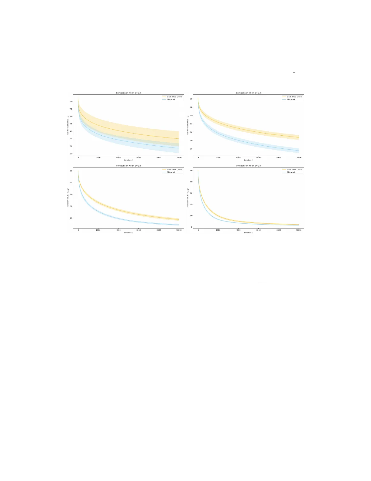
Clipp ed Gradien t Metho ds for Nonsmo oth Con v ex Optimization under Hea vy-T ailed Noise: A Reﬁned Analysis ∗ Zijian Liu † Abstract Optimization under hea vy-tailed noise has b ecome popular recently , since it b etter ﬁts man y mo dern mac hine learning tasks, as captured by empirical observ ations. Concretely , instead of a ﬁnite second momen t on gradient noise, a b ounded p -th momen t where p ∈ (1 , 2] has b een recognized to be more realistic (sa y b eing upp er bounded by σ p l for some σ l ≥ 0 ). A simple yet eﬀectiv e op eration, gradient clipping, is kno wn to handle this new challenge successfully . Sp eciﬁcally , Clipp ed Stochastic Gradient De- scen t (Clipp ed SGD) guaran tees a high-probability rate O ( σ l ln(1 /δ ) T 1 p − 1 ) (resp. O ( σ 2 l ln 2 (1 /δ ) T 2 p − 2 ) ) for nonsmo oth con vex (resp. strongly con vex) problems, where δ ∈ (0 , 1] is the failure probability and T ∈ N is the time horizon. In this w ork, we provide a reﬁned analysis for Clipp ed SGD and oﬀer t wo faster rates, O ( σ l d − 1 2 p eﬀ ln 1 − 1 p (1 /δ ) T 1 p − 1 ) and O ( σ 2 l d − 1 p eﬀ ln 2 − 2 p (1 /δ ) T 2 p − 2 ) , than the aforemen tioned b est results, where d eﬀ ≥ 1 is a quantit y we call the gener alize d eﬀe ctive dimension . Our analysis improv es up on the existing approach in tw o resp ects: b etter utilization of F reedman’s inequality and ﬁner b ounds for clipping error under hea vy-tailed noise. In addition, we extend the reﬁned analysis to con vergence in exp ectation and obtain new rates that break the known lo wer bounds. Lastly , to complement the study , w e establish new low er b ounds for b oth high-probability and in-exp ectation conv ergence. Notably , the in- exp ectation low er b ounds match our new upp er bounds, indicating the optimality of our reﬁned analysis for con v ergence in expectation. 1 In tro duction In ﬁrst-order metho ds for sto c hastic optimization, one can only query an unbiased though noisy gradient and then implement a gradien t descent step, which is known as Sto c hastic Gradient Descen t (SGD) (Robbins and Monro, 1951). Under the widely assumed ﬁnite v ariance condition, i.e., the gradien t noise 1 has a ﬁnite second momen t, the in-expectation conv ergence of SGD has b een substan tially studied (Bottou et al., 2018; Lan, 2020). Ho wev er, many recen t empirical observ ations suggest that the ﬁnite v ariance assumption might b e to o strong and could b e violated in diﬀerent tasks (Simsekli et al., 2019; Zhang et al., 2020; Zhou et al., 2020; Garg et al., 2021; Gurbuzbalaban et al., 2021; Ho dgkinson and Mahoney, 2021; Battash et al., 2024). Instead, a b ounded p -th moment condition where p ∈ (1 , 2] (say with an upp er b ound σ p l for some σ l ≥ 0 ) b etter ﬁts mo dern mac hine learning, which is named heavy-tailed noise. F acing this new c hallenge, SGD has been pro ved to exhibit undesirable behaviors (Zhang et al., 2020; Sadiev et al., 2023). Therefore, an algorithmic c hange is necessary . A simple y et eﬀectiv e op eration, gradient clipping, is kno wn to handle this harder situation successfully with b oth fav orable practical p erformance and pro v able theoretical guarantees (see, e.g., P ascanu et al. (2013); Zhang et al. (2020)). The clipping mechanism replaces the sto c hastic gradien t g t in ev ery iterate of SGD with its truncated counterpart clip τ t ( g t ) , resulting a metho d kno wn as Clipp ed SGD, where τ t is called the clipping threshold and clip τ ( g ) ≜ min { 1 , τ / ∥ g ∥ } g is the clipping function. Sp eciﬁcally , for nonsmo oth conv ex (resp. strongly conv ex) optimization, Clipp ed SGD ac hieves a high- probabilit y rate O ( σ l ln(1 /δ ) T 1 p − 1 ) 2 (resp. O ( σ 2 l ln 2 (1 /δ ) T 2 p − 2 ) ) (Liu and Zhou, 2023), where δ ∈ (0 , 1] is ∗ A preliminary conference version is accepted at ICLR 2026. Compared to the conference v ersion, we include the formal statements of low er b ounds and their pro ofs. Moreov er, the upp er b ounds are slightly improv ed. † Stern School of Business, New Y ork Universit y , zl3067@stern.nyu.edu. 1 This refers to the diﬀerence b et ween the sto c hastic estimate and the true gradient. 2 When stating rates in this section, we only keep the dominant term when T → ∞ and δ → 0 for simplicity . 1 the failure probability and T ∈ N is the time horizon. These t wo results seem to be optimal as they matc h the existing in-exp ectation low er b ounds (Nemiro vski and Y udin, 1983; V ural et al., 2022; Zhang et al., 2020), if viewing the p oly(ln(1 /δ )) term as a constant. How ev er, a recent adv ance (Das et al., 2024) established a b etter rate O ( σ l d − 1 4 eﬀ p ln(ln( T ) /δ ) /T ) for general con vex problems when p = 2 , where 1 ≤ d eﬀ ≤ d is kno wn as the eﬀe ctive dimension (also named intrinsic dimension (T ropp, 2015)) and d is the true dimension. This rev eals that the in-expectation lo w er bound does not necessarily apply to the term containing p oly(ln(1 /δ )) . More imp ortan tly , such a result hin ts that a general impro vemen t may exist for all p ∈ (1 , 2] . This work conﬁrms that a general improv emen t do es exist b y pro viding a reﬁned analysis for Clipp ed SGD. Concretely , we oﬀer t wo faster rates, O ( σ l d − 1 2 p eﬀ ln 1 − 1 p (1 /δ ) T 1 p − 1 ) for general con vex problems with a kno wn T and O ( σ 2 l d − 1 p eﬀ ln 2 − 2 p (1 /δ ) T 2 p − 2 ) for strongly conv ex problems with an unknown T , impro v ed up on the aforementioned b est results, where 1 ≤ d eﬀ ≤ O ( d ) is a quantit y that w e call the gener alize d eﬀe ctive dimension 3 . Moreo v er, we devise an algorithmic v ariant of Clipp ed SGD named Stabilized Clipp ed SGD that achiev es the same rate 4 for conv ex ob jectives listed ab o ve in an anytime fashion, i.e., no extra poly (ln T ) factor even without T . W e highlight that our analysis impro ves up on the existing approach in tw o resp ects: 1. W e observ e a b etter w ay to apply F reedman’s inequalit y when analyzing Clipp ed SGD, which leads to a prov ably tighter concen tration. Remark ably , our approac h is fairly simple in con trast to the previous complex iterativ e reﬁnemen t strategy (Das et al., 2024). 2. W e establish ﬁner b ounds for clipping error under heavy-tailed noise, whic h is another essential ingredient in the analysis for Clipp ed SGD when the noise has a heavy tail. W e believe b oth of these new insights could be of independent interest and potentially useful for future researc h. F urthermore, equipp ed with the new ﬁner b ounds for clipping error, w e extend the analysis to in- exp ectation conv ergence and obtain t wo new rates, O ( σ l d − 2 − p 2 p eﬀ T 1 p − 1 ) for general conv ex ob jectiv es and O ( σ 2 l d − 2 − p p eﬀ T 2 p − 2 ) for strongly conv ex problems. Notably , once p < 2 , these tw o rates are b oth faster by a p oly(1 /d eﬀ ) factor than the kno wn optimal low er b ounds Ω( σ l T 1 p − 1 ) and Ω( σ 2 l T 2 p − 2 ) in the corresp onding setting (Nemirovski and Y udin, 1983; V ural et al., 2022; Zhang et al., 2020). Lastly , to complemen t the study , w e establish new lo wer b ounds for b oth high-probability and in- exp ectation conv ergence. Notably , the in-exp ectation lo wer b ounds match our new upp er b ounds, indicating the optimality of our reﬁned analysis for conv ergence in exp ectation. 1.1 Related W ork W e review the literature that studies nonsmo oth (strongly) conv ex optimization under hea vy-tailed noise. F or other diﬀerent settings, e.g., smo oth (strongly) con vex or smo oth/nonsmooth nonconv ex problems under hea vy-tailed noise, the in terested reader could refer to, for example, Nazin et al. (2019); Davis and Drusvy- atskiy (2020); Gorbuno v et al. (2020); Mai and Johansson (2021); Cutkosky and Meh ta (2021); W ang et al. (2021); T sai et al. (2022); Holland (2022); Jako vetić et al. (2023); Sadiev et al. (2023); Liu et al. (2023); Nguy en et al. (2023); Puchkin et al. (2024); Gorbunov et al. (2024b); Liu et al. (2024); Armacki et al. (2025); Hübler et al. (2025); Liu and Zhou (2025); Sun et al. (2025), for recent progress. High-probabilit y rates. If p = 2 , Gorbunov et al. (2024a) prov es the ﬁrst O ( σ l p ln( T /δ ) /T ) (resp. O ( σ 2 l ln( T /δ ) /T ) ) high-probabilit y rate for nonsmooth con vex (resp. strongly con vex) problems under stan- dard assumptions. If additionally assuming a b ounded domain, an improv ed rate O ( σ l p ln(1 /δ ) /T ) for con vex ob jectiv es is obtained b y P arletta et al. (2024). Still for con vex problems, Das et al. (2024) re- cen tly gives the ﬁrst reﬁned b ound O ( σ l d − 1 4 eﬀ p ln(ln( T ) /δ ) /T ) but additionally requiring T ≥ Ω(ln(ln d )) , where d eﬀ (resp. d ) is the eﬀectiv e (resp. true) dimension, satisfying 1 ≤ d eﬀ ≤ d . F or general p ∈ (1 , 2] , Zhang and Cutkosky (2022) studies the harder online conv ex optimization, whose result implies a rate O ( σ l p oly(ln( T /δ )) T 1 p − 1 ) for heavy-tailed conv ex optimization. Later on, Liu and Zhou (2023) establishes t wo bounds, O ( σ l ln(1 /δ ) T 1 p − 1 ) and O ( σ 2 l ln 2 (1 /δ ) T 2 p − 2 ) , for conv ex and strongly conv ex problems, resp ec- 3 W e use the same notation to denote the eﬀectiv e dimension and the generalized version prop osed b y us, since our new quantit y can recov er the previous one when p = 2 . See discussion after (1) for details. 4 T o clarify , “the same rate” refers to the same low er-order term. The full b ound is slightly diﬀerent. 2 tiv ely . These tw o rates are the b est-kno wn results for general p ∈ (1 , 2] and ha v e b een recognized as optimal since they match the in-exp ectation lo wer b ounds (see below), if viewing the p oly(ln(1 /δ )) term as a constant. In-exp ectation rates. Note that the in-exp ectation rates for p = 2 are not w orth muc h attention as they are standard results (Bottou et al., 2018; Lan, 2020). As for general p ∈ (1 , 2] , many existing works pro ve the rates O ( σ l T 1 p − 1 ) and O ( σ 2 l T 2 p − 2 ) (Zhang et al., 2020; V ural et al., 2022; Liu and Zhou, 2023, 2024; P arletta et al., 2025; F atkh ullin et al., 2025; Liu, 2025). Lo wer b ounds. The high-probabilit y lo wer b ounds are not fully explored in the literature. T o the b est of our knowledge, there are only few results for the general con vex case and no lo wer b ounds for the strongly con vex case. Therefore, the follo wing discussion is only for conv ex problems. F or p = 2 , Carmon and Hinder (2024) shows a low er b ound Ω( σ l p ln(1 /δ ) /T ) . How ev er, it is only pro ved for d = 1 (or at most d = 4 ). As suc h, it cannot reveal useful information for the case that d should also b e viewed as a parameter (if more accurately , d eﬀ ). In other words, it do es not con tradict our new reﬁned upp er bound. F or general p ∈ (1 , 2] , Raginsky and Rakhlin (2009) is the only work that we are a ware of. Ho wev er, as far as we can c heck, only the time horizon T is in the right order of Ω( T 1 p − 1 ) . F or other parameters, they are either hidden or not tigh t. Next, we summarize the in-exp ectation low er b ounds. F or conv ex problems, it is known that any ﬁrst- order method cannot do b etter than Ω( σ l T 1 p − 1 ) (Nemiro vski and Y udin, 1983; V ural et al., 2022). If strong con vexit y additionally holds, Zhang et al. (2020) establishes the low er b ound Ω( σ 2 l T 2 p − 2 ) . 2 Preliminary Notation. N is the set of natural num b ers (excluding 0 ). W e denote by [ T ] ≜ { 1 , · · · , T } , ∀ T ∈ N . ⟨· , ·⟩ represen ts the standard Euclidean inner product. ∥ x ∥ is the Euclidean norm of the v ector x and ∥ X ∥ is the op erator norm of the matrix X . T r( X ) is the trace of a square matrix X . S d − 1 stands for the unit sphere in R d . Giv en a conv ex function h : R d → R , ∇ h ( x ) denotes an arbitrary element in ∂ h ( x ) where ∂ h ( x ) is the subgradien t set of h at x . sgn( x ) is the sign function with sgn(0) = 0 . W e study the comp osite optimization problem in the form of inf x ∈ X F ( x ) ≜ f ( x ) + r ( x ) , where X ⊆ R d is a nonempty closed con vex set. Our analysis relies on the following assumptions. Assumption 1. Ther e exists x ⋆ ∈ X such that F ⋆ ≜ F ( x ⋆ ) = inf x ∈ X F ( x ) . Assumption 2. Both f : R d → R and r : R d → R ar e c onvex. In addition, r is µ -str ongly c onvex on X for some µ ≥ 0 , i.e., r ( x ) ≥ r ( y ) + ⟨∇ r ( y ) , x − y ⟩ + µ 2 ∥ x − y ∥ 2 , ∀ x , y ∈ X . Assumption 3. f is G -Lipschitz on X , i.e., ∥∇ f ( x ) ∥ ≤ G, ∀ x ∈ X . The ab o ve assumptions are standard in the literature (Bottou et al., 2018; Nesterov et al., 2018; Lan, 2020). Next, w e consider a ﬁne-grained heavy-tailed noise assumption, the key to obtaining reﬁned conv er- gence for Clipp ed SGD. Assumption 4. Ther e exists a function g : X × Ξ → R d and a pr ob ability distribution D on Ξ such that E ξ ∼ D [ g ( x , ξ )] = ∇ f ( x ) , ∀ x ∈ X . In addition, for some p ∈ (1 , 2] , we have E ξ ∼ D  |⟨ e , g ( x , ξ ) − ∇ f ( x ) ⟩| p  ≤ σ p s , E ξ ∼ D  ∥ g ( x , ξ ) − ∇ f ( x ) ∥ p  ≤ σ p l , ∀ x ∈ X , e ∈ S d − 1 , wher e σ s and σ l ar e two c onstants satisfying 0 ≤ σ s ≤ σ l ≤ p π d/ 2 σ s . R emark 1 . In the remaining paper, if the context is clear, we drop the subscript ξ ∼ D in E ξ ∼ D to ease the notation. Moreo v er, d ( x , ξ ) ≜ g ( x , ξ ) − ∇ f ( x ) denotes the error in estimating the gradient. R emark 2 . It is notew orthy that Assumption 4 actually implicitly exists in prior w orks for heavy-tailed sto c hastic optimization, since Cauch y-Sch w arz inequality giv es us E  |⟨ e , d ( x , ξ ) ⟩| p  ≤ E  ∥ e ∥ p ∥ d ( x , ξ ) ∥ p  = E  ∥ d ( x , ξ ) ∥ p  , ∀ x ∈ X , e ∈ S d − 1 . 3 In other w ords, once the condition E  ∥ d ( x , ξ ) ∥ p  ≤ σ p l , ∀ x ∈ X is assumed lik e in prior w orks, there m ust exist a real num b er 0 ≤ σ s ≤ σ l suc h that E  |⟨ e , d ( x , ξ ) ⟩| p  ≤ σ p s , ∀ x ∈ X , e ∈ S d − 1 . R emark 3 . The reason we can assume σ l ≤ p π d/ 2 σ s is that E  ∥ d ( x , ξ ) ∥ p  ≤ ( π d/ 2) p 2 σ p s holds provided E  |⟨ e , d ( x , ξ ) ⟩| p  ≤ σ p s , ∀ e ∈ S d − 1 , due to Lemma 4.1 in Cherapanamjeri et al. (2022). No w w e deﬁne the following quantit y named gener alize d eﬀe ctive dimension (where we use the conv ention 0 = 0 / 0 ), d eﬀ ≜ σ 2 l /σ 2 s ∈ { 0 } ∪ [1 , π d/ 2] = O ( d ) , (1) in which d eﬀ = 0 if and only if σ l = σ s = 0 , i.e., the noiseless case. As discussed later, this deﬁnition recov ers the eﬀective dimension used in Das et al. (2024) when p = 2 . T o b etter understand Assumption 4, we ﬁrst take p = 2 . Note that a ﬁnite second momen t of d ( x , ξ ) implies the cov ariance matrix Σ( x ) ≜ E  d ( x , ξ ) d ⊤ ( x , ξ )  ∈ R d × d is well deﬁned. As such, we can in terpret σ l and σ s as σ 2 l = sup x ∈ X T r(Σ( x )) and σ 2 s = sup x ∈ X ∥ Σ( x ) ∥ . In particular, if Σ( x ) ⪯ Σ , ∀ x ∈ X holds for some p ositiv e semideﬁnite Σ as assumed in Das et al. (2024), then one can directly take σ 2 l = T r(Σ) and σ 2 s = ∥ Σ ∥ , which also reco vers the eﬀectiv e dimension deﬁned as T r(Σ) / ∥ Σ ∥ in Das et al. (2024). F or general p ∈ (1 , 2] , as discussed in Remark 2, one can view Assumption 4 as a ﬁner version of the classical heavy-tailed noise condition, the latter omits the existence of σ s . Therefore, Assumption 4 describ es the b eha vior of noise more precisely . Such reﬁnemen t w as only introduced to the classical mean estimation problem (Cherapanamjeri et al., 2022) as far as we know, and hence is new to the optimization literature. In App endix A, w e provide more discussions on how large d eﬀ can b e across diﬀeren t settings. 3 Clipp ed Sto c hastic Gradien t Descen t Algorithm 1 Clipped Sto chastic Gradien t Descent (Clipped SGD) Input: initial point x 1 ∈ X , stepsize η t > 0 , clipping threshold τ t > 0 for t = 1 to T do g c t = clip τ t ( g t ) where g t = g ( x t , ξ t ) and ξ t ∼ D is sampled indep enden tly from the history x t +1 = argmin x ∈ X r ( x ) + ⟨ g c t , x ⟩ + ∥ x − x t ∥ 2 2 η t end for W e present the main metho d studied in this work, Clipp ed Sto chastic Gradient Descen t (Clipp ed SG D), in Algorithm 1. Strictly sp eaking, the algorithm should b e called Proximal Clipp ed SGD as it contains a pro ximal up date step. How ev er, we drop the word “Pro ximal” for simplicity . W e remark that Clipped SGD with a pro ximal step has not b een fully studied yet and is diﬀerent from the Pro x-Clipp ed-SGD-Shift metho d in tro duced in Gorbunov et al. (2024b), the only work considering comp osite optimization under heavy-tailed noise that we are a ware of. In comparison to the classical Pro ximal SGD, Algorithm 1 only contains an extra clipping operation on the sto c hastic gradien t. As p oin ted out in prior works (e.g., Sadiev et al. (2023)), the additional clipping step is the key to pro ving the high-probabilit y conv ergence. 4 Reﬁned High-Probabilit y Rates In this section, we will establish reﬁned high-probabilit y conv ergence results for Clipp ed SGD. T o simplify the notation in the up coming theorems, we denote b y D ≜ ∥ x ⋆ − x 1 ∥ the distance b et w een the optimal solution and the initial p oint. Moreov er, giv en δ ∈ (0 , 1] , we in tro duce the quantit y τ ⋆ ≜ min ( σ s σ p − 1 l ln 3 δ , σ 2 s σ 2 − p l 1 [ p < 2] )! 1 p , (2) 4 whic h is an imp ortan t v alue used in the clipping threshold. Recall that d eﬀ = σ 2 l /σ 2 s , then τ ⋆ can be equiv alently written into τ ⋆ = σ l /φ 1 / p ⋆ where φ ⋆ ≜ max  p d eﬀ ln 3 δ , d eﬀ 1 [ p < 2]  . (3) 4.1 General Con v ex Case W e start from the general conv ex case (i.e., µ = 0 in Assumption 2). ¯ x cvx T +1 ≜ 1 T P T t =1 x t +1 in the following denotes the av erage iterate after T steps. T o clarify , T is assumed to b e known in adv ance in this subsection. Though Clipped SGD can prov ably handle an unknown time horizon T , it is w ell-known to incur extra p oly(ln T ) factors (Liu and Zhou, 2023). T o deal with this issue, w e propose a v ariant of Clipped SGD named Stabilized Clipp ed SGD in App endix C, whic h incorporates the stabilization tric k in tro duced b y F ang et al. (2022). As an example, Theorem 11 in App endix E shows that Stabilized Clipp ed SGD conv erges at an almost identical rate to Theorem 1 below, but in an an ytime fashion without incurring any p oly(ln T ) factor. Theorem 1. Under Assumptions 1, 2 (with µ = 0 ), 3 and 4, for any T ∈ N and δ ∈ (0 , 1] , setting η t = η ⋆ , τ t = max n 2 G, τ ⋆ T 1 p o , ∀ t ∈ [ T ] wher e η ⋆ is a pr op erly picke d stepsize (explic ate d in The or em 10), then Clipp e d SGD (A lgorithm 1) guar ante es that with pr ob ability at le ast 1 − δ , F ( ¯ x cvx T +1 ) − F ⋆ c onver ges at the r ate of O   ( φ + ln 3 δ ) GD T + GD √ T + ( σ 2 p − 1 s σ 2 − 2 p l + σ 1 p s σ 1 − 1 p l ln 1 − 1 p 3 δ ) D T 1 − 1 p   , wher e φ ≤ φ ⋆ is a c onstant (explic ate d in The or em 10) and e quals φ ⋆ when T = Ω  G p σ p l φ ⋆  . T o better understand Theorem 1, we ﬁrst consider a special case of p = 2 (i.e., the classical ﬁnite v ariance condition) and obtain a rate b eing at most O  ( √ d eff +1) ln( 1 δ ) GD T + ( G + σ l + √ σ s σ l ln( 1 δ )) D √ T  . In com- parison, the previous best high-probabilit y b ound in the ﬁnite v ariance setting pro ved b y Das et al. (2024) is O  C T + ( √ d eff + G σ s ) ln( ln T δ ) GD T + ( G + σ l + √ σ s ( σ l + G ) ln( ln T δ )) D √ T  , but under an extra requiremen t T ≥ Ω(ln(ln d )) , where C T is a term in the order of O ( T − 3 2 ) but will blo w up to + ∞ when the v ariance approaches 0 . As one can see, even in this special case, our result immediately improv es upon Das et al. (2024) from the follo wing three folds: 1. Our theory w orks for any time horizon T ∈ N . 2. Our b ound is strictly b etter than theirs b y shaving oﬀ many redundant terms. Esp ecially , the dep endence on δ is only ln(1 /δ ) in contrast to their ln((ln T ) /δ ) . 3. Our rate will not blow up when σ l → 0 (equiv alently , σ s → 0 ) and instead recov er the standard O ( GD/ √ T ) result for deterministic nonsmo oth con vex optimization (Nestero v et al., 2018). Next, the prior best result for p ∈ (1 , 2] is O  GD ln 1 δ √ T + σ l D ln 1 δ T 1 − 1 p  (Liu and Zhou, 2023), whose dominan t term is O ( σ l D ln(1 /δ ) T 1 p − 1 ) as T b ecomes larger. In comparison, using d eﬀ = σ 2 l /σ 2 s , the low er-order term in Theorem 1 can b e written as O ( σ l D ( d 1 2 − 1 p eﬀ + d − 1 2 p eﬀ ln 1 − 1 p (1 /δ )) T 1 p − 1 ) . Therefore, Theorem 1 improv es up on Liu and Zhou (2023) for large T by a factor of ρ ≜ Θ   d 1 2 − 1 p eﬀ + d − 1 2 p eﬀ ln 1 − 1 p 1 δ ln 1 δ   = Θ   1 d 2 − p 2 p eﬀ ln 1 δ + 1 d 1 2 p eﬀ ln 1 p 1 δ   . (4) R emark 4 . Esp ecially , when d eﬀ = Ω( d ) , ρ could be in the order of Θ(poly (1 /d, 1 / ln(1 /δ ))) . W e pro vide an example in App endix A showing that d eﬀ = Ω( d ) is attainable. F or general T ∈ N , note that O ( GD ln(1 /δ ) /T + last tw o terms ) in Theorem 1 are alwa ys smaller than the rate of Liu and Zhou (2023) due to σ s ≤ σ l . Therefore, w e only need to pay atten tion to the redundan t 5 term O ( φGD/T ) . Observe that a critical time could b e T ⋆ = Θ( φ 2 ⋆ ) = Θ( d eﬀ ln 2 (1 /δ ) + d 2 eﬀ 1 [ p < 2]) 5 . Once T ≥ T ⋆ , we can ignore O ( φGD/T ) as it is at most O ( GD / √ T ) now. It is currently unknown whether the term O ( φGD/T ) is inevitable or can b e remov ed to obtain a b etter b ound than Liu and Zhou (2023) for an y T ∈ N . W e remark that similar additional terms also appear in the reﬁned rate for p = 2 b y Das et al. (2024) as discussed b efore. 4.2 Strongly Con v ex Case W e no w mov e to the strongly conv ex case (i.e., µ > 0 in Assumption 2). ¯ x str T +1 ≜ P T t =1 ( t +4)( t +5) x t +1 P T t =1 ( t +4)( t +5) in the follo wing denotes the w eighted av erage iterate after T steps. Unlik e the general con vex case, w e do not need to know T in adv ance to remo ve the extra p oly(ln T ) factor. Theorem 2. Under Assumptions 1, 2 (with µ > 0 ), 3 and 4, for any T ∈ N and δ ∈ (0 , 1] , setting η t = 6 µt , τ t = max n 2 G, τ ⋆ t 1 p o , ∀ t ∈ [ T ] , then Clipp e d SGD (Algorithm 1) guar ante es that with pr ob ability at le ast 1 − δ , b oth F ( ¯ x str T +1 ) − F ⋆ and µ ∥ x T +1 − x ⋆ ∥ 2 c onver ge at the r ate of O   µD 2 T 3 +  φ 2 + ln 2 3 δ  G 2 µT 2 + G 2 µT + σ 4 p − 2 s σ 4 − 4 p l + σ 2 p s σ 2 − 2 p l ln 2 − 2 p 3 δ µT 2 − 2 p   , wher e φ ≤ φ ⋆ is the same c onstant as in The or em 1 and e quals φ ⋆ when T = Ω  G p σ p l φ ⋆  . R emark 5 . The problem studied in prior works (e.g., Liu and Zhou (2023); Gorbuno v et al. (2024a)) considers strongly conv ex and Lipschitz f with r = 0 , whic h seems diﬀerent from our assumption of strongly con vex r . Ho wev er, a simple reduction can con vert their instance to ﬁt our setting. Moreov er, the ﬁrst term O ( µD 2 /T 3 ) in Theorem 2 can also b e omitted in that case (as we will do so in the follo wing discussion). W e refer the in terested reader to App endix B for the reduction and why the term O ( µD 2 /T 3 ) can b e ignored. T o sa ve space, w e only compare with the rate O  G 2 ln 2 1 δ µT + ( σ 2 l + σ p l G 2 − p ) ln 2 1 δ µT 2 − 2 p  (Liu and Zhou, 2023) for general p ∈ (1 , 2] . F or the sp ecial case p = 2 , the rate of Liu and Zhou (2023) is almost identical to the b ound of Gorbunov et al. (2024a); moreov er, as far as we know, no improv ed result like Das et al. (2024) has b een obtained to give a b etter b ound for the term containing p oly(ln(1 /δ )) . Similar to the discussion after Theorem 1, one can ﬁnd that for large T , the improv ement ov er Liu and Zhou (2023) is at least by a factor of ρ 2 (4) = Θ   1 d 2 − p p eﬀ ln 2 1 δ + 1 d 1 p eﬀ ln 2 p 1 δ   = Θ  p oly  1 d eﬀ , 1 ln 1 δ  . F or general T ∈ N , every term in Theorem 2 is still b etter except for O ( φ 2 G 2 / ( µT 2 )) . Ho wev er, this extra term has no eﬀect once T ≥ T ⋆ = Θ( φ 2 ⋆ ) = Θ( d eﬀ ln 2 (1 /δ ) + d 2 eﬀ 1 [ p < 2]) , the same critical time for Theorem 1 (a similar discussion to F o otnote 5 also applies here), since it is at most O ( G 2 / ( µT )) now, b eing dominated b y other terms. Same as b efore, it is unclear whether this redundan t term O ( φ 2 G 2 / ( µT 2 )) can b e shav ed oﬀ to conclude a faster rate for any T ∈ N or not. W e lea ve it as fu ture work and look forward to it being addressed. 5 Pro of Sk etch and New Insigh ts In this section, w e sk etch the proof of Theorem 1 as an example and in tro duce our new insigh ts in the analysis. T o start wi th, giv en T ∈ N and supp ose η t = η , τ t = τ , ∀ t ∈ [ T ] for simplicit y , we hav e the following 5 Actually , any T ⋆ that makes O ( φGD/T ) in Theorem 1 smaller than the sum of the terms left is enough. Hence, it is possible to ﬁnd a smaller critical time. W e keep this one here due to its clear expression. 6 inequalit y for Clipp ed SGD (see Lemma 4 in App endix F), which holds almost surely without any restriction on τ , F ( ¯ x cvx T +1 ) − F ⋆ ≤ D 2 η + 2 I cvx T , where I cvx T is a residual term in the order of I cvx T = O       η       max t ∈ [ T ] t X s =1 ⟨ d u s , y s ⟩ ! 2 | {z } I + T X t =1 ∥ d u t ∥ 2 | {z } II + T X t =1   d b t   ! 2 | {z } II I + G 2 T             , (5) in whic h d u t ≜ g c t − E t − 1 [ g c t ] and d b t ≜ E t − 1 [ g c t ] − ∇ f ( x t ) resp ectiv ely denote the un biased and biased part in the clipping error, where E t [ · ] ≜ E [ · | F t ] for F t ≜ σ ( ξ 1 , · · · , ξ t ) b eing the natural ﬁltration, and y t is some predictable vector (i.e., y t ∈ F t − 1 ) satisfying ∥ y t ∥ ≤ 1 almost surely . The term η G 2 T in I cvx T is standard. Hence, the left task is to b ound terms I , I I and II I in high probability . In particular, for I and II I , we will mo ve b ey ond the existing approach via a reﬁned analysis. T o formalize the diﬀerence, we borrow the following bounds for clipping error commonly used in the literature (see, e.g., Sadiev et al. (2023); Liu and Zhou (2023); Nguyen et al. (2023)): ∥ d u t ∥ ≤ O ( τ ) , E t − 1 h ∥ d u t ∥ 2 i if τ ≥ 2 G ≤ O ( σ p l τ 2 − p ) ,   d b t   if τ ≥ 2 G ≤ O ( σ p l τ 1 − p ) . (6) T erm I . Note that X t ≜ ⟨ d u t , y t ⟩ is a martingale diﬀerence sequence (MDS), then F reedman’s inequal- it y (Lemma 10 in App endix F) implies with probabilit y at least 1 − δ , √ I ≤ O (max t ∈ [ T ] | X t | ln(1 /δ ) + q P T t =1 E t − 1 [ X 2 t ] ln(1 /δ )) (this inequalit y is for illustration, not entirely rigorous in math). T o the b est of our kno wledge, prior works studying Clipp ed SGD under heavy-tailed noise alwa ys b ound similar terms in the following manner | X t | ∥ y t ∥≤ 1 ≤ ∥ d u t ∥ (6) ≤ O ( τ ) and E t − 1  X 2 t  ∥ y t ∥≤ 1 ≤ E t − 1 h ∥ d u t ∥ 2 i (6) ≤ O ( σ p l τ 2 − p ) . Ho wev er, a critical observ ation is that the ab ov e-described widely adopted w ay is v ery likely to be loose, as the conditional v ariance can b e b etter con trolled by E t − 1  X 2 t  = y ⊤ t E t − 1  d u t ( d u t ) ⊤  y t ∥ y t ∥≤ 1 ≤   E t − 1  d u t ( d u t ) ⊤    . Note that   E t − 1  d u t ( d u t ) ⊤    is at most E t − 1 h ∥ d u t ∥ 2 i but could be m uch smaller. Inspired b y this, we dev elop a new b ound for   E t − 1  d u t ( d u t ) ⊤    in Lemma 1. Consequently , this better utilization of F reedman’s inequalit y concludes a tigh ter high-probability b ound for term I . A ctually , this simple but eﬀective idea has b een implicitly used in Das et al. (2024) when p = 2 . How ev er, their pro of ﬁnally falls complex due to an argument they call the iterative reﬁnement strategy , which not only imp oses extra undesired factors like ln((ln T ) /δ ) in their ﬁnal b ound but also leads to an additional requiremen t T ≥ Ω(ln(ln d )) in their theory . Our analysis indicates that suc h a complication is unnecessary , instead, one can keep it simple. T erm I I . F or this term, w e follo w the same wa y emplo yed in man y previous w orks (e.g., Cutkosky and Mehta (2021); Zhang and Cutkosky (2022)), i.e., let X t ≜ ∥ d u t ∥ 2 − E t − 1 h ∥ d u t ∥ 2 i and decomp ose P T t =1 ∥ d u t ∥ 2 (6) ≤ O ( P T t =1 X t + σ p l τ 2 − p T ) then use F reedman’s inequalit y to b ound P T t =1 X t . R emark 6 . Although the abov e analysis follo ws the literature, we still obtain a reﬁned inequalit y for E t − 1 h ∥ d u t ∥ 2 i in Lemma 1, in the sense of dropping the condition τ ≥ 2 G required in (6). T erm I II . Estimating the clipping error   d b t   is another k ey ingredient when analyzing Clipped SGD. As far as we kno w, all existing w orks apply the inequality   d b t   ≤ O ( σ p l τ 1 − p ) in (6). How ev er, w e sho w that 7 this imp ortan t inequality still has ro om for impro vemen t. In other words, it is in fact not tight, as revealed b y our ﬁner b ounds in Lemma 1. Th us, our result is more reﬁned. F rom the ab ov e discussion, in addition to b etter utilization of F reedman’s inequalit y , the improv ement hea vily relies on ﬁner b ounds for clipping error under hea vy-tailed noise, whic h we give in the follo wing Lemma 1. Lemma 1. Under Assumptions 3 and 4, and assuming τ t = τ > 0 , ther e ar e: ∥ d u t ∥ ≤ O ( τ ) ,   E t − 1  d u t ( d u t ) ⊤    if τ ≥ 2 G ≤ O ( σ p s τ 2 − p + σ p l G 2 τ − p ) , E t − 1 h ∥ d u t ∥ 2 i ≤ O ( σ p l τ 2 − p ) ,   d b t   if τ ≥ 2 G ≤ O ( σ s σ p − 1 l τ 1 − p + σ p l Gτ − p ) . R emark 7 . W e highligh t that Theorem 9 in App endix D pro vides a further generalization of clipping error b ounds under heavy-tailed noise not limited to clipped gradient metho ds (even without the requirement in the form of τ ≥ 2 G ), which could b e potentially useful for future research. Except for the standard bound ∥ d u t ∥ ≤ O ( τ ) , the other three inequalities in Lemma 1 are either new or impro ve o ver the existing results. 1. The b ound on   E t − 1  d u t ( d u t ) ⊤    is new in the heavy-tailed setting. Imp ortan tly , observ e that O ( σ p s τ 2 − p + σ p l G 2 τ − p ) ≤ O ( σ p l τ 2 − p ) due to σ s ≤ σ l and τ ≥ 2 G , whic h thereby leads to a tigh ter high-probabilit y b ound for term I in combination with our b etter application of F reedman’s inequalit y (see the paragraph b efore starting with T erm I . ). 2. F or term E t − 1 h ∥ d u t ∥ 2 i , in contrast to (6), Lemma 1 remo ves the condition τ ≥ 2 G . Moreov er, the hidden constant in our lemma is actually slightly b etter. 3. As mentioned abov e (see the paragraph b efore starting with T erm I II . ), the b ound of   d b t   is another k ey to obtainin g a reﬁned result. Precisely , we note that the new b ound O ( σ s σ p − 1 l τ 1 − p + σ p l Gτ − p ) impro ves up on O ( σ p l τ 1 − p ) in (6) b ecause of σ s ≤ σ l and τ ≥ 2 G . Therefore, Lemma 1 guarantees a b etter con trol for term I II . Com bining all the new insights mentioned, we can ﬁnally pro ve Theorem 1. As one can imagine, the analysis sketc hed ab o v e is essen tially more reﬁned than previous w orks, since we apply tighter b ounds for the t wo central parts in analyzing Clipp ed SGD, i.e., concentration inequalities and estimation of clipping error. T o conﬁrm this claim, we discuss ho w to reco ver the existing rate through our ﬁner analysis, the details of whic h are deferred to App endix E. Lastly , w e men tion that Theorem 2 for strongly conv ex problems is also inspired b y the abov e t wo new insigh ts. The full pro ofs of b oth Theorems 1 and 2 can b e found in App endix E. 6 Extension to F aster In-Exp ectation Con v ergence In this section, we show that Lemma 1 presen ted b efore can also lead to faster in-exp ectation conv ergence for Clipp ed SGD, further highligh ting the v alue of reﬁned clipping error b ounds. Pro ofs of b oth theorems giv en b elow can be found in App endix E. This time, we consider a new quantit y e τ ⋆ ≜ σ 2 p s / ( σ 2 p − 1 l 1 [ p < 2]) for the clipping threshold. Recall that d eﬀ = σ 2 l /σ 2 s , then e τ ⋆ can b e equiv alently written in to e τ ⋆ = σ l / e φ 1 / p ⋆ where e φ ⋆ ≜ d eﬀ 1 [ p < 2] . (7) R emark 8 . When p = 2 , e φ ⋆ = 0 ⇒ e τ ⋆ = + ∞ , i.e., no clipping op eration is required. This matches the w ell-known fact that SGD prov ably conv erges in exp ectation under the ﬁnite v ariance condition. 6.1 General Con v ex Case Theorem 3. Under Assumptions 1, 2 (with µ = 0 ), 3 and 4, for any T ∈ N , setting η t = η ⋆ , τ t = max n 2 G, e τ ⋆ T 1 p o , ∀ t ∈ [ T ] wher e η ⋆ is a pr op erly picke d stepsize (explic ate d in The or em 12), then Clipp e d SGD (A lgorithm 1) guar ante es that E  F ( ¯ x cvx T +1 ) − F ⋆  c onver ges at the r ate of O   e φGD T + GD √ T + σ 2 p − 1 s σ 2 − 2 p l D T 1 − 1 p   , 8 wher e e φ ≤ e φ ⋆ is a c onstant (explic ate d in The or em 12) and e quals e φ ⋆ when T = Ω  G p σ p l e φ ⋆  . Theorem 3 gives a b etter lo wer-order term O ( σ l d 1 2 − 1 p eﬀ D T 1 p − 1 ) (recall d eﬀ = σ 2 l /σ 2 s ) than the existing lo wer b ound Ω( σ l D T 1 p − 1 ) (Nemirovski and Y udin, 1983; V ural et al., 2022) by a factor of Θ(1 /d 2 − p 2 p eﬀ ) , a strict improv ement b eing p olynomial in 1 /d eﬀ , if p ∈ (1 , 2) . F or the case of an unknown T , the interested reader could refer to Theorem 13 in App endix E. 6.2 Strongly Con v ex Case Theorem 4. Under Assumptions 1, 2 (with µ > 0 ), 3 and 4, for any T ∈ N , setting η t = 6 µt , τ t = max n 2 G, e τ ⋆ t 1 p o , ∀ t ∈ [ T ] , then Clipp e d SGD (Algorithm 1) guar ante es that b oth E  F ( ¯ x str T +1 ) − F ⋆  and µ E h ∥ x T +1 − x ⋆ ∥ 2 i c onver ge at the r ate of O   µD 2 T 3 + e φ 2 G 2 µT 2 + G 2 µT + σ 4 p − 2 s σ 4 − 4 p l µT 2 − 2 p   , wher e e φ ≤ e φ ⋆ is the same c onstant as in The or em 3 and e quals e φ ⋆ when T = Ω  G p σ p l e φ ⋆  , Theorem 4 pro vides a faster rate O ( σ 2 l d 1 − 2 p eﬀ T 2 p − 2 ) than the known low er b ound Ω( σ 2 l T 2 p − 2 ) (Zhang et al., 2020) by a factor of Θ(1 /d 2 − p p eﬀ ) , this is again a strict improv ement once p < 2 , and could b e in the order of p oly(1 /d ) if d eﬀ = Ω( d ) . 7 Lo w er Bounds T o complemen t the study , we pro vide new high-probabilit y and in-exp ectation lo wer bounds for b oth µ = 0 and µ > 0 . W e employ information-theoretic metho ds to establish these new low er b ounds, following the existing literature (Raginsky and Rakhlin, 2009; Agarw al et al., 2012; Duc hi et al., 2013; V ural et al., 2022; Carmon and Hinder, 2024; Ma et al., 2024). F or complete pro ofs, the in terested reader could refer to App endix G. R emark 9 . One may wonder wh y our upper b ounds can b eat the existing lo w er b ounds, and also where the diﬀerence betw een our new low er bounds and the prior ones lies. The key is our ﬁne-grained Assumption 4. Roughly sp eaking, the existing lo wer b ounds are prov ed for the follo wing oracle class (we sligh tly abuse the notation by still using g to denote the sto c hastic gradient oracle), G p σ l = n g : R d × f → R d : E [ g ( x ,f ) | x ,f ]= ∇ f ( x ) ∈ ∂ f ( x ) E [ ∥ g ( x ,f ) −∇ f ( x ) ∥ p | x ,f ] ≤ σ p l , ∀ x ∈ R d , f ∈ f o , where p ∈ (1 , 2] and σ l ≥ 0 are tw o parameters and f is the function class that w e are interested in (e.g., the family of G -Lipsc hitz con vex functions). In con trast, the oracle class we study is parameterized b y one more parameter σ s ∈ h σ l / p π d/ 2 , σ l i as follows, G p σ s ,σ l ≜ ( g : R d × f → R d : E [ g ( x ,f ) | x ,f ]= ∇ f ( x ) ∈ ∂ f ( x ) E [ |⟨ e , g ( x ,f ) −∇ f ( x ) ⟩| p | x ,f ] ≤ σ p s , ∀ e ∈ S d − 1 E [ ∥ g ( x ,f ) −∇ f ( x ) ∥ p | x ,f ] ≤ σ p l , ∀ x ∈ R d , f ∈ f ) . Note that there is G p σ s ,σ l ⊆ G p σ l , implying the lo wer b ound pro ved for G p σ l could b e lo ose for G p σ s ,σ l . Therefore, our upp er b ounds can surpass the existing lo wer bounds, and our new low er b ounds are established for the ﬁne-grained oracle class G p σ s ,σ l . 9 7.1 High-Probabilit y Lo w er Bounds Theorem 5 (Informal version of Theorem 16) . Under Assumptions 1, 2 (with µ = 0 ), 3 and 4, assuming d ≥ d eﬀ ≥ 1 and δ ∈  0 , 1 10  , any algorithm c onver ges at le ast at the r ate of Ω ( σ 2 p − 1 s σ 2 − 2 p l + σ s ln 1 − 1 p 1 δ ) D T 1 − 1 p ! with pr ob ability at le ast δ when T is lar ge enough. Theorem 6 (Informal version of Theorem 17) . Under Assumptions 1, 2 (with µ > 0 ), 3 and 4, assuming d ≥ d eﬀ ≥ 1 and δ ∈  0 , 1 10  , any algorithm c onver ges at le ast at the r ate of Ω σ 4 p − 2 s σ 4 − 4 p l + σ 2 s ln 2 − 2 p 1 δ µT 2 − 2 p ! with pr ob ability at le ast δ when T is lar ge enough. Compared to our upp er b ounds in high probability , i.e., Theorems 1 ( µ = 0 ) and 2 ( µ > 0 ), there are still diﬀerences b et ween the terms that contain the p oly(ln(1 /δ )) factor. Closing this imp ortan t gap is an in teresting task, whic h we lea ve for future w ork. 7.2 In-Exp ectation Low er Bounds Theorem 7 (Informal version of Theorem 18) . Under Assumptions 1, 2 (with µ = 0 ), 3 and 4, assuming d ≥ d eﬀ ≥ 1 , any algorithm c onver ges at le ast at the r ate of Ω σ 2 p − 1 s σ 2 − 2 p l D T 1 − 1 p ! in exp e ctation when T is lar ge enough. Theorem 8 (Informal version of Theorem 19) . Under Assumptions 1, 2 (with µ > 0 ), 3 and 4, assuming d ≥ d eﬀ ≥ 1 , any algorithm c onver ges at le ast at the r ate of Ω σ 4 p − 2 s σ 4 − 4 p l µT 2 − 2 p ! in exp e ctation when T is lar ge enough. F or in-exp ectation conv ergence, the ab o ve lo wer b ounds match our new upp er b ounds, i.e., Theorems 3 ( µ = 0 ) and 4 ( µ > 0 ), indicating the optimality of our reﬁned analysis for con vergence in expectation. 8 Conclusion and F uture W ork In this work, we provide a reﬁned analysis of Clipp ed SGD and obtain faster high-probability rates than the previously best-known b ounds. The impro vemen t is achiev ed b y b etter utilization of F reedman’s in- equalit y and ﬁner b ounds for clipping error under heavy-tailed noise. Moreo ver, w e extend the analysis to in-exp ectation con vergence and show new rates that break the existing low er b ounds. T o complement the study , we establish new low er b ounds for b oth high-probability and in-exp ectation conv ergence. Notably , the in-exp ectation upp er and low er b ounds match each other, indicating the optimalit y of our reﬁned analysis for conv ergence in exp ectation. There are still some directions w orth exploring in the future, which w e list b elo w: The extra term. Eac h of our reﬁned rates has a highe r-order term related to d eﬀ (e.g., O ( φGD/T ) in Theorem 1 and O ( φ 2 G 2 / ( µT 2 )) in Theorem 2). Although it is negligible when T is large, proving/dispro ving it can b e remo ved for an y T ∈ N could be an in teresting task. Gaps in high-probabilit y b ounds. As discussed in Section 7, there are still gaps betw een high- probabilit y upp er and low er b ounds for b oth conv ex and strongly conv ex cases. Closing them is an imp ortan t direction for the future. Other optimization problems. W e remark that our tw o new insigh ts are not limited to nonsmo oth con vex problems. Instead, they are general concepts/results. Therefore, we believe that it is p ossible to apply them to other optimization problems under heavy-tailed noise (e.g., smo oth (strongly) conv ex/noncon vex problems) and obtain improv ed upp er b ounds faster than existing ones. 10 References Alekh Agarwal, Peter L. Bartlett, Pradeep Ravikumar, and Martin J. W ainwrigh t. Information-theoretic lo wer b ounds on the oracle complexity of sto c hastic con v ex optimization. IEEE T r ansactions on Informa- tion The ory , 58(5):3235–3249, 2012. doi: 10.1109/TIT.2011.2182178. Aleksandar Armac ki, Sh uhua Y u, Pranay Sharma, Gauri Joshi, Dragana Ba jo vic, Dusan Jak ov etic, and Soumm ya Kar. High-probability conv ergence bounds for online nonlinear stochastic gradient descent under heavy-tailed noise. In Yingzhen Li, Stephan Mandt, Shipra Agraw al, and Emtiy az Khan, editors, Pr o c e e dings of The 28th International Confer enc e on Artiﬁcial Intel ligenc e and Statistics , v olume 258 of Pr o c e e dings of Machine L e arning R ese ar ch , pages 1774–1782. PMLR, 03–05 May 2025. URL https: //proceedings.mlr.press/v258/armacki25a.html . Barak Battash, Lior W olf, and Oﬁr Lindenbaum. Revisiting the noise mo del of sto c hastic gradient descent. In Sanjo y Dasgupta, Stephan Mandt, and Yingzhen Li, editors, Pr o c e e dings of The 27th International Con- fer enc e on Artiﬁcial Intel ligenc e and Statistics , volume 238 of Pr o c e e dings of Machine L e arning R ese ar ch , pages 4780–4788. PMLR, 02–04 Ma y 2024. URL https://proceedings.mlr.press/v238/battash24a. html . Amir Beck and Marc T eb oulle. Mirror descen t and nonlinear pro jected subgradient metho ds for con- v ex optimization. Op er ations R ese ar ch L etters , 31(3):167–175, 2003. ISSN 0167-6377. doi: https: //doi.org/10.1016/S0167- 6377(02)00231- 6. URL https://www.sciencedirect.com/science/article/ pii/S0167637702002316 . Léon Bottou, F rank E. Curtis, and Jorge Nocedal. Optimization metho ds for large-scale machine learn- ing. SIAM R eview , 60(2):223–311, 2018. doi: 10.1137/16M1080173. URL https://doi.org/10.1137/ 16M1080173 . J. Bretagnolle and C. Hub er. Estimation des densités: risque minimax. Zeitschrift für W ahrscheinlichkeit- sthe orie und V erwandte Gebiete , 47(2):119–137, 1979. ISSN 1432-2064. doi: 10.1007/BF00535278. URL https://doi.org/10.1007/BF00535278 . D. L. Burkholder. Distribution F unction Inequalities for Martingales. The Annals of Pr ob ability , 1(1):19 – 42, 1973. doi: 10.1214/aop/1176997023. URL https://doi.org/10.1214/aop/1176997023 . Y air Carmon and Oliv er Hinder. The price of adaptivit y in sto c hastic con v ex optimization. In Shipra Agra wal and Aaron Roth, editors, Pr o c e e dings of Thirty Seventh Confer enc e on L e arning The ory , volume 247 of Pr o c e e dings of Machine L e arning R ese ar ch , pages 772–774. PMLR, 30 Jun–03 Jul 2024. URL https://proceedings.mlr.press/v247/carmon24a.html . Y eshw anth Cherapanamjeri, Nilesh T ripuraneni, Peter Bartlett, and Michael Jordan. Optimal mean esti- mation without a v ariance. In Po-Ling Loh and Maxim Raginsky , editors, Pr o c e e dings of Thirty Fifth Confer enc e on L e arning The ory , volume 178 of Pr o c e e dings of Machine L e arning R ese ar ch , pages 356–357. PMLR, 02–05 Jul 2022. URL https://proceedings.mlr.press/v178/cherapanamjeri22a.html . Ashok Cutkosky and Harsh Mehta. High-probabilit y b ounds for non-conv ex sto c hastic optimization with hea vy tails. In M. Ranzato, A. Beygelzimer, Y. Dauphin, P .S. Liang, and J. W ortman V aughan, editors, A dvanc es in Neur al Information Pr o c essing Systems , v olume 34, pages 4883–4895. Cur- ran Asso ciates, Inc., 2021. URL https://proceedings.neurips.cc/paper_files/paper/2021/file/ 26901debb30ea03f0aa833c9de6b81e9- Paper.pdf . Anik et Das, Dheera j Nagara j, Soum yabrata Pal, Arun Sai Suggala, and Prateek V arshney . Near-optimal streaming heavy-tailed statistical estimation with clipp ed sgd. In A. Glob erson, L. Mac key , D. Belgrav e, A. F an, U. Paquet, J. T omczak, and C. Zhang, editors, A dvanc es in Neur al Information Pr o c essing Systems , v olume 37, pages 8834–8900. Curran Asso ciates, Inc., 2024. URL https://proceedings.neurips.cc/ paper_files/paper/2024/file/10bf96894abaf4c293b205709a98fc74- Paper- Conference.pdf . 11 Damek Davis and Dmitriy Drusvyatskiy . High probability guarantees for sto c hastic conv ex optimization. In Jacob Ab erneth y and Shiv ani Agarwal, editors, Pr o c e e dings of Thirty Thir d Confer enc e on L e arning The ory , volume 125 of Pr o c e e dings of Machine L e arning R ese ar ch , pages 1411–1427. PMLR, 09–12 Jul 2020. URL https://proceedings.mlr.press/v125/davis20a.html . John Duchi, Michael I Jordan, and Brendan McMahan. Estimation, optimization, and paral- lelism when data is sparse. In C.J. Burges, L. Bottou, M. W elling, Z. Ghahramani, and K.Q. W einberger, editors, A dvanc es in Neur al Information Pr o c essing Systems , v olume 26. Cur- ran Asso ciates, Inc., 2013. URL https://proceedings.neurips.cc/paper_files/paper/2013/file/ 2812e5cf6d8f21d69c91dddeefb792a7- Paper.pdf . Ric k Durrett. Pr ob ability: The ory and Examples . Cam bridge Series in Statistical and Probabilistic Mathe- matics. Cambridge Univ ersit y Press, 5 edition, 2019. Huang F ang, Nic holas J. A. Harvey , Victor S. Portella, and Michael P . F riedlander. Online mirror descent and dual av eraging: Keeping pace in the dynamic case. Journal of Machine L e arning R ese ar ch , 23(121): 1–38, 2022. URL http://jmlr.org/papers/v23/21- 1027.html . Ily as F atkhullin, Florian Hübler, and Guanghui Lan. Can sgd handle heavy-tailed noise? arXiv pr eprint arXiv:2508.04860 , 2025. Da vid A. F reedman. On T ail Probabilities for Martingales. The Annals of Pr ob ability , 3(1):100 – 118, 1975. doi: 10.1214/aop/1176996452. URL https://doi.org/10.1214/aop/1176996452 . Saurabh Garg, Joshua Zhanson, Emilio Parisotto, A darsh Prasad, Zico K olter, Zachary Lipton, Siv ara- man Balakrishnan, Ruslan Salakh utdinov, and Pradeep Ravikumar. On proximal p olicy optimization’s hea vy-tailed gradients. In Marina Meila and T ong Zhang, editors, Pr o c e e dings of the 38th International Confer enc e on Machine L e arning , volume 139 of Pr o c e e dings of Machine L e arning R ese ar ch , pages 3610– 3619. PMLR, 18–24 Jul 2021. URL https://proceedings.mlr.press/v139/garg21b.html . E. N. Gilb ert. A comparison of signalling alphab ets. The Bel l System T e chnic al Journal , 31(3):504–522, 1952. doi: 10.1002/j.1538- 7305.1952.tb01393.x. Eduard Gorbunov, Marina Danilov a, and Alexander Gasniko v. Sto chastic optimization with heavy-tailed noise via accelerated gradien t clipping. In H. Laro c helle, M. Ranzato, R. Hadsell, M.F. Balcan, and H. Lin, editors, A dvanc es in Neur al Information Pr o c essing Systems , v olume 33, pages 15042–15053. Cur- ran Asso ciates, Inc., 2020. URL https://proceedings.neurips.cc/paper_files/paper/2020/file/ abd1c782880cc59759f4112fda0b8f98- Paper.pdf . Eduard Gorbuno v, Marina Danilo v a, Innok en tiy Shibaev, Pa v el Dvurec hensky , and Alexander Gasnik ov. High-probabilit y complexity b ounds for non-smo oth stochastic con vex optimization with heavy-tailed noise. Journal of Optimization The ory and Applic ations , pages 1–60, 2024a. Eduard Gorbuno v, Ab durakhmon Sadiev, Marina Danilo v a, Samuel Horv áth, Gauthier Gidel, P av el Dvurec hensky , Alexander Gasnik ov, and Peter Ric htárik. High-probability conv ergence for composite and distributed sto c hastic minimization and v ariational inequalities with heavy-tailed noise. In Ruslan Salakh utdinov, Zico K olter, Katherine Heller, Adrian W eller, Nuria Oliver, Jonathan Scarlett, and F e- lix Berkenk amp, editors, Pr o c e e dings of the 41st International Confer enc e on Machine L e arning , volume 235 of Pr o c e e dings of Machine L e arning R ese ar ch , pages 15951–16070. PMLR, 21–27 Jul 2024b. URL https://proceedings.mlr.press/v235/gorbunov24a.html . Mert Gurbuzbalaban, Umut Simsekli, and Ling jiong Zhu. The heavy-tail phenomenon in sgd. In Marina Meila and T ong Zhang, editors, Pr o c e e dings of the 38th International Confer enc e on Machine L e arning , v olume 139 of Pr o c e e dings of Machine L e arning R ese ar ch , pages 3964–3975. PMLR, 18–24 Jul 2021. URL https://proceedings.mlr.press/v139/gurbuzbalaban21a.html . Liam Ho dgkinson and Michael Mahoney . Multiplicative noise and heavy tails in sto c hastic optimization. In Marina Meila and T ong Zhang, editors, Pr o c e e dings of the 38th International Confer enc e on Machine 12 L e arning , v olume 139 of Pr o c e e dings of Machine L e arning R ese ar ch , pages 4262–4274. PMLR, 18–24 Jul 2021. URL https://proceedings.mlr.press/v139/hodgkinson21a.html . Matthew J. Holland. Anytime guarantees under hea vy-tailed data. Pr o c e e dings of the AAAI Confer enc e on A rtiﬁcial Intel ligenc e , 36(6):6918–6925, Jun. 2022. doi: 10.1609/aaai.v36i6.20649. URL https://ojs. aaai.org/index.php/AAAI/article/view/20649 . Florian Hübler, Ily as F atkhullin, and Niao He. F rom gradien t clipping to normalization for hea vy tailed sgd. In Yingzhen Li, Stephan Mandt, Shipra Agraw al, and Em tiyaz Khan, editors, Pr o c e e dings of The 28th International Confer enc e on Artiﬁcial Intel ligenc e and Statistics , volume 258 of Pr o c e e dings of Machine L e arning R ese ar ch , pages 2413–2421. PMLR, 03–05 May 2025. URL https://proceedings.mlr.press/ v258/hubler25a.html . Maor Ivgi, Oliv er Hinder, and Y air Carmon. DoG is SGD’s b est friend: A parameter-free dynamic step size schedule. In Andreas Krause, Emma Brunskill, Kyungh yun Cho, Barbara Engelhardt, Siv an Sabato, and Jonathan Scarlett, editors, Pr o c e e dings of the 40th International Confer enc e on Machine L e arning , v olume 202 of Pr o c e e dings of Machine L e arning R ese ar ch , pages 14465–14499. PMLR, 23–29 Jul 2023. URL https://proceedings.mlr.press/v202/ivgi23a.html . Dušan Jako vetić, Dragana Ba jović, Anit Kumar Sahu, Soummy a Kar, Nemanja Milošević, and Dušan Sta- menk ović. Nonlinear gradient mappings and sto c hastic optimization: A general framework with applica- tions to heavy-tail noise. SIAM Journal on Optimization , 33(2):394–423, 2023. doi: 10.1137/21M145896X. URL https://doi.org/10.1137/21M145896X . Guangh ui Lan. First-or der and sto chastic optimization metho ds for machine le arning . Springer, 2020. Langqi Liu, Yib o W ang, and Lijun Zhang. High-probability b ound for non-smo oth non-conv ex sto c hastic optimization with heavy tails. In Ruslan Salakhutdino v, Zico Kolter, Katherine Heller, Adrian W eller, Nuria Oliv er, Jonathan Scarlett, and F elix Berk enk amp, editors, Pr o c e e dings of the 41st International Confer enc e on Machine L e arning , v olume 235 of Pr o c e e dings of Machine L e arning R ese ar ch , pages 32122– 32138. PMLR, 21–27 Jul 2024. URL https://proceedings.mlr.press/v235/liu24bo.html . Zijian Liu. Online conv ex optimization with heavy tails: Old algorithms, new regrets, and applications. arXiv pr eprint arXiv:2508.07473 , 2025. Zijian Liu and Zhengyuan Zhou. Sto c hastic nons mooth con v ex optimization with hea vy-tailed noises: High- probabilit y b ound, in-exp ectation rate and initial distance adaptation. arXiv pr eprint arXiv:2303.12277 , 2023. Zijian Liu and Zhengyuan Zhou. Revisiting the last-iterate con vergence of stochastic gradient metho ds. In The Twelfth International Confer enc e on L e arning R epr esentations , 2024. URL https://openreview. net/forum?id=xxaEhwC1I4 . Zijian Liu and Zhengyuan Zhou. Nonconv ex sto c hastic optimization under heavy-tailed noises: Optimal con vergence without gradient clipping. In The Thirte enth International Confer enc e on L e arning R epr e- sentations , 2025. URL https://openreview.net/forum?id=NKotdPUc3L . Zijian Liu, Jiaw ei Zhang, and Zhengyuan Zhou. Breaking the low er b ound with (little) structure: Acceleration in non-con vex stochastic optimization with hea vy-tailed noise. In Gergely Neu and Lorenzo Rosasco, editors, Pr o c e e dings of Thirty Sixth Confer enc e on L e arning The ory , volume 195 of Pr o c e e dings of Machine L e arning R ese ar ch , pages 2266–2290. PMLR, 12–15 Jul 2023. URL https://proceedings.mlr.press/ v195/liu23c.html . Tian yi Ma, Kabir A V erc hand, and Richard J Samw orth. High-probability minimax low er b ounds. arXiv pr eprint arXiv:2406.13447 , 2024. Vien V. Mai and Mik ael Johansson. Stabilit y and conv ergence of stochastic gradien t clipping: Beyond lipsc hitz contin uit y and smo othness. In Marina Meila and T ong Zhang, editors, Pr o c e e dings of the 38th International Confer enc e on Machine L e arning , v olume 139 of Pr o c e e dings of Machine L e arning R ese ar ch , pages 7325–7335. PMLR, 18–24 Jul 2021. URL https://proceedings.mlr.press/v139/mai21a.html . 13 Alexander V Nazin, Ark adi S Nemirovsky , Alexandre B T sybako v, and Anatoli B Juditsky . Algorithms of robust sto c hastic optimization based on mirror descen t method. A utomation and R emote Contr ol , 80(9): 1607–1627, 2019. Ark adi Nemiro vski and David Y udin. Problem complexity and metho d eﬃciency in optimization. Wiley- Interscienc e , 1983. Y urii Nestero v et al. L e ctur es on c onvex optimization , volume 137. Springer, 2018. T a Duy Nguy en, Thien H Nguyen, Alina Ene, and Huy Nguyen. Improv ed conv ergence in high probabilit y of clipp ed gradien t metho ds with heavy tailed noise. In A. Oh, T. Naumann, A. Glob erson, K. Saenk o, M. Hardt, and S. Levine, editors, A dvanc es in Neur al Information Pr o c essing Systems , v olume 36, pages 24191–24222. Curran Associates, Inc., 2023. URL https://proceedings.neurips.cc/paper_files/ paper/2023/file/4c454d34f3a4c8d6b4ca85a918e5d7ba- Paper- Conference.pdf . John P Nolan. Univariate stable distributions . Springer, 2020. Daniela Angela P arletta, Andrea P audice, Massimiliano Pon til, and Sa verio Salzo. High probabilit y b ounds for stochastic subgradient schemes with heavy tailed noise. SIAM Journal on Mathematics of Data Scienc e , 6(4):953–977, 2024. doi: 10.1137/22M1536558. URL https://doi.org/10.1137/22M1536558 . Daniela Angela Parletta, Andrea P audice, and Sa verio Salzo. An improv ed analysis of the clipp ed sto c hastic subgradien t metho d under heavy-tailed noise, 2025. URL . Razv an P ascanu, T omas Mik olov, and Y oshua Bengio. On the diﬃculty of training recurren t neural netw orks. In Sanjoy Dasgupta and David McAllester, editors, Pr o c e e dings of the 30th International Confer enc e on Machine L e arning , volume 28 of Pr o c e e dings of Machine L e arning R ese ar ch , pages 1310–1318, A tlanta, Georgia, USA, 17–19 Jun 2013. PMLR. URL https://proceedings.mlr.press/v28/pascanu13.html . Nikita Puchkin, Eduard Gorbunov, Nick ola y Kutuzov, and Alexander Gasniko v. Breaking the hea vy-tailed noise barrier in sto c hastic optimization problems. In Sanjoy Dasgupta, Stephan Mandt, and Yingzhen Li, editors, Pr o c e e dings of The 27th International Confer enc e on Artiﬁcial Intel ligenc e and Statistics , v olume 238 of Pr o c e e dings of Machine L e arning R ese ar ch , pages 856–864. PMLR, 02–04 Ma y 2024. URL https://proceedings.mlr.press/v238/puchkin24a.html . Maxim Raginsky and Alexander Rakhlin. Information complexity of blac k-b o x con v ex optimization: A new lo ok via feedback information theory . In 2009 47th Annual Al lerton Confer enc e on Communic ation, Contr ol, and Computing (Al lerton) , pages 803–510, 2009. doi: 10.1109/ALLER TON.2009.5394945. Herb ert Robbins and Sutton Monro. A Sto c hastic Appro ximation Metho d. The Annals of Mathematic al Statistics , 22(3):400 – 407, 1951. doi: 10.1214/aoms/1177729586. URL https://doi.org/10.1214/aoms/ 1177729586 . Ab durakhmon Sadiev, Marina Danilov a, Eduard Gorbunov, Sam uel Horv áth, Gauthier Gidel, Pa vel Dvurec hensky , Alexander Gasniko v, and P eter Ric htárik. High-probabilit y bounds for stochastic opti- mization and v ariational inequalities: the case of unbounded v ariance. In Andreas Krause, Emma Brun- skill, Kyunghyun Cho, Barbara Engelhardt, Siv an Sabato, and Jonathan Scarlett, editors, Pr o c e e dings of the 40th International Confer enc e on Machine L e arning , volume 202 of Pr o c e e dings of Machine L e arning R ese ar ch , pages 29563–29648. PMLR, 23–29 Jul 2023. URL https://proceedings.mlr.press/v202/ sadiev23a.html . Gennady Samoro dnitsky and Murad S T aqqu. Stable non-Gaussian r andom pr o c esses: sto chastic mo dels with inﬁnite varianc e , volume 1. CR C press, 1994. Um ut Simsekli, Leven t Sagun, and Mert Gurbuzbalaban. A tail-index analysis of sto c hastic gradien t noise in deep neural net works. In Kamalik a Chaudhuri and Ruslan Salakh utdinov, editors, Pr o c e e dings of the 36th International Confer enc e on Machine L e arning , volume 97 of Pr o c e e dings of Machine L e arning R ese ar ch , pages 5827–5837. PMLR, 09–15 Jun 2019. URL https://proceedings.mlr.press/v97/simsekli19a. html . 14 T ao Sun, Xinw ang Liu, and Kun Y uan. Revisiting gradient normalization and clipping for nonconv ex sgd under heavy-tailed noise: Necessity , s uﬃciency , and acceleration. Journal of Machine L e arning R ese ar ch , 26(237):1–42, 2025. URL http://jmlr.org/papers/v26/24- 1991.html . Jo el A. T ropp. An introduction to matrix concentration inequalities. F oundations and T r ends ® in Machine L e arning , 8(1-2):1–230, 2015. ISSN 1935-8237. doi: 10.1561/2200000048. URL http://dx.doi.org/10. 1561/2200000048 . Che-Ping T sai, Adarsh Prasad, Siv araman Balakrishnan, and Pradeep Ravikumar. Hea vy-tailed streaming statistical estimation. In Gustau Camps-V alls, F rancisco J. R. Ruiz, and Isab el V alera, editors, Pr o c e e dings of The 25th International Confer enc e on Artiﬁcial Intel ligenc e and Statistics , volume 151 of Pr o c e e dings of Machine L e arning R ese ar ch , pages 1251–1282. PMLR, 28–30 Mar 2022. URL https://proceedings. mlr.press/v151/tsai22a.html . Rom Rub eno vich V arshamov. The ev aluation of signals in co des with correction of errors. In Doklady A kademii Nauk , volume 117, pages 739–741. Russian Academ y of Sciences, 1957. Nuri Mert V ural, Lu Y u, Krishna Balasubramanian, Stanislav V olgushev, and Murat A Erdogdu. Mirror descen t strikes again: Optimal sto c hastic conv ex optimization under inﬁnite noise v ariance. In Po-Ling Loh and Maxim Raginsky , editors, Pr o c e e dings of Thirty Fifth Confer enc e on L e arning The ory , volume 178 of Pr o c e e dings of Machine L e arning R ese ar ch , pages 65–102. PMLR, 02–05 Jul 2022. URL https: //proceedings.mlr.press/v178/vural22a.html . Hong jian W ang, Mert Gurbuzbalaban, Ling jiong Zh u, Umut Simsekli, and Murat A Erdogdu. Con ver- gence rates of sto chastic gradient descent under inﬁnite noise v ariance. In M. Ranzato, A. Beygelzimer, Y. Dauphin, P .S. Liang, and J. W ortman V aughan, editors, A dvanc es in Neur al Information Pr o c essing Systems , v olume 34, pages 18866–18877. Curran Asso ciates, Inc., 2021. URL https://proceedings. neurips.cc/paper_files/paper/2021/file/9cdf26568d166bc6793ef8da5afa0846- Paper.pdf . Manfred K W armuth, Arun K Jagota, et al. Con tinuous and discrete-time nonlinear gradien t descen t: Relativ e loss b ounds and conv ergence. In Ele ctr onic pr o c e e dings of the 5th International Symp osium on A rtiﬁcial Intel ligenc e and Mathematics , volume 326. Citeseer, 1997. Jingzhao Zhang, Sai Praneeth Karimireddy , Andreas V eit, Seungyeon Kim, Sashank Reddi, Sanjiv Kumar, and Suvrit Sra. Why are adaptive metho ds go od for attention mo dels? In H. Laro c helle, M. Ranzato, R. Hadsell, M.F. Balcan, and H. Lin, editors, A dvanc es in Neur al Information Pr o c essing Systems , v ol- ume 33, pages 15383–15393. Curran Associates, Inc., 2020. URL https://proceedings.neurips.cc/ paper_files/paper/2020/file/b05b57f6add810d3b7490866d74c0053- Paper.pdf . Jiujia Zhang and Ashok Cutkosky . P arameter-free regret in high probabilit y with heavy tails. In S. Ko yejo, S. Mohamed, A. Agarwal, D. Belgrav e, K. Cho, and A. Oh, editors, A d- vanc es in Neur al Information Pr o c essing Systems , v olume 35, pages 8000–8012. Curran As- so ciates, Inc., 2022. URL https://proceedings.neurips.cc/paper_files/paper/2022/file/ 349956dee974cfdcbbb2d06afad5dd4a- Paper- Conference.pdf . P an Zhou, Jiashi F eng, Chao Ma, Caiming Xiong, Stev en Chu Hong Hoi, and W einan E. T ow ards theoreti- cally understanding why sgd generalizes b etter than adam in deep learning. In H. Laro c helle, M. Ranzato, R. Hadsell, M.F. Balcan, and H. Lin, editors, A dvanc es in Neur al Information Pr o c essing Systems , v ol- ume 33, pages 21285–21296. Curran Associates, Inc., 2020. URL https://proceedings.neurips.cc/ paper_files/paper/2020/file/f3f27a324736617f20abbf2ffd806f6d- Paper.pdf . Vladimir M Zolotarev. One-dimensional stable distributions , volume 65. American Mathematical Soc., 1986. 15 A Lo w er Bounds on d eﬀ This section provides low er b ounds on d eﬀ for the additive noise mo del, i.e., g ( x , ξ ) = ∇ f ( x ) + ξ . Given i ∈ [ d ] , ξ i denotes the i -th co ordinate of ξ , and σ i ≜  E  | ξ i | p  1 p is the p -th moment of ξ i . Additionally , ι : [ d ] → [ d ] is the p erm utation that makes σ i in a nonincreasing order, i.e., σ ι 1 ≥ σ ι 2 ≥ · · · ≥ σ ι d − 1 ≥ σ ι d . A.1 Indep enden t Co ordinates In this subsection, we assume that all of ξ i are mutually independent. • F or any j ∈ [ d ] , w e can lo wer bound ∥ ξ ∥ p = d X i =1 ξ 2 i ! p 2 ≥ j X i =1 ξ 2 ι i ! p 2 ≥ j p 2 − 1 j X i =1 | ξ ι i | p , where the last step is by the concavit y of x p 2 , which implies σ p l = E  ∥ ξ ∥ p  ≥ j p 2 − 1 P j i =1 σ p ι i . Therefore, w e can ﬁnd σ p l ≥ max j ∈ [ d ] j p 2 − 1 j X i =1 σ p ι i . (8) • F or any e ∈ S d − 1 , we write e = P d i =1 λ i e i where P d i =1 λ 2 i = 1 and e i denotes the all-zero vector except for the i -th co ordinate, which is one. Therefore, we ha ve E  |⟨ e , ξ ⟩| p  = E        d X i =1 λ i ξ i      p   ( a ) ≤ 2 2 − p d X i =1 E  | λ i ξ i | p  = 2 2 − p d X i =1 | λ i | p σ p i ( b ) ≤ 2 2 − p d X i =1 σ 2 p 2 − p i ! 1 − p 2 , where ( a ) holds by | a + b | p ≤ | a | p + p | a | p − 1 sgn( a ) b + 2 2 − p | b | p (see Prop osition 18 of V ural et al. (2022)) and the mutual independence of ξ i , and ( b ) is due to d X i =1 | λ i | p σ p i ≤ d X i =1 λ 2 i ! p 2 d X i =1 σ 2 p 2 − p i ! 1 − p 2 = d X i =1 σ 2 p 2 − p i ! 1 − p 2 . Hence, we kno w σ p s = sup e ∈ S d − 1 E  |⟨ e , ξ ⟩| p  ≤ 2 2 − p d X i =1 σ 2 p 2 − p i ! 1 − p 2 . (9) As such, w e can low er b ound d eﬀ = σ 2 l σ 2 s (8) , (9) ≥ max j ∈ [ d ] j 1 − 2 p  P j i =1 σ p ι i  2 p 2 4 p − 2  P d i =1 σ 2 p 2 − p i  2 p − 1 . (10) Though (10) do es not direc tly giv e a lo wer b ound for d eﬀ expressed in terms of d , it has already provided some useful information. F or example, when σ i are all in the same order, (10) implies that d eﬀ = Ω  d 2 − 2 p  . A.2 I.I.D. Co ordinates In this subsection, w e further assume that all ξ i are i.i.d. and then low er b ound d eﬀ b y d . Since all coordinates are identically distributed no w, we write σ i = σ, ∀ i ∈ [ d ] for some σ ≥ 0 in the follo wing. 16 A.2.1 A General Ω( d 2 − 2 p ) Bound W e in vok e (10) and plug in σ i = σ to obtain d eﬀ (10) ≥ max j ∈ [ d ] j σ 2 2 4 p − 2 d 2 p − 1 σ 2 = d 2 − 2 p 2 4 p − 2 . (11) When p = 2 , the ab o ve bound recov ers the fact that d eﬀ = d for ξ with i.i.d. coordinates. A.2.2 A Sp ecial Ω( d ) Bound No w we consider a sp ecial kind of noise. Suppose p ∈ (1 , 2) and all ξ i ha ve the c haracteristic function E [exp (i tξ i )] = exp  − γ α | t | α  1 − i β tan  π α 2  sgn( t )  , ∀ t ∈ R , where α = p + ϵ for ϵ ∈ (0 , 2 − p ] , β ∈ [ − 1 , 1] , and γ ≥ 0 . Suc h a distribution is known as α -stable distribution satisfying that E [ ξ i ] = 0 , σ < ∞ , and P d i =1 ξ i equals to d 1 α ξ 1 in distribution (Zolotarev, 1986; Samoro dnitsky and T aqqu, 1994; Nolan, 2020). This suggests that w e can lo wer bound σ p l in another wa y , σ p l = E  ∥ ξ ∥ p  = E   d X i =1 ξ 2 i ! p 2   ≥ E     P d i =1 ξ i    p  18 p p p  p p − 1  p 2 = E     d 1 α ξ 1    p  18 p p p  p p − 1  p 2 = d p p + ϵ σ p 18 p p p  p p − 1  p 2 , (12) where the inequality is due to Burkholder (1973). Therefore, in this sp ecial case, we ha ve d eﬀ = σ 2 l σ 2 s (9) , (12) ≥ d 2 p + ϵ σ 2  18 2 p 3 p − 1 2 4 p − 2 d 2 p − 1 σ 2 = ( p − 1) d 1 − 2 ϵ p ( p + ϵ ) p 3 3 4 2 4 p . (13) In particular, for any 0 < ϵ ≤ min n p 2 ln d − 1 , 2 − p o (assume d ≥ 2 here, since the case d = 1 is trivial), 2 ϵ p ( p + ϵ ) ≤ 1 p ln d ⇒ d 2 ϵ p ( p + ϵ ) ≤ e 1 p ⇒ d eﬀ (13) ≥ ( p − 1) d p 3 3 4 2 4 p e 1 p = Ω( d ) . (14) B Reduction for Strongly Con v ex Problems W e provide the reduction mentioned in Remark 5. Recall that existing works assume f b eing µ -strongly con vex and G -Lipschitz with a minimizer x ⋆ on X . Now w e consider the following problem instance to ﬁt our problem structure F ( x ) = f ( x ) − µ 2 ∥ x − y ∥ 2 | {z } ≜ ¯ f ( x ) + µ 2 ∥ x − y ∥ 2 | {z } ≜ r ( x ) = f ( x ) , where y can b e an y known p oin t in X . F or example, one can set y = x 1 to b e the initial p oin t. Next, we sho w that F fulﬁlls all assumptions in Section 2. • F on X has the same optimal solution x ⋆ as f and hence satisﬁes Assumption 1. • Note that ¯ f is conv ex (since f is µ -strongly conv ex) and r is µ -strongly conv ex, whic h ﬁts Assumption 2. • Moreov er, because f is µ -strongly con vex and G -Lipsc hitz with a minimizer x ⋆ ∈ X , a w ell-know fact is that X has to be bounded, since for an y x ∈ X , µ 2 ∥ x − x ⋆ ∥ 2 ≤ f ( x ) − f ( x ⋆ ) − ⟨∇ f ( x ⋆ ) , x − x ⋆ ⟩ ≤ f ( x ) − f ( x ⋆ ) ≤ ⟨∇ f ( x ) , x − x ⋆ ⟩ ≤ ∥∇ f ( x ) ∥ ∥ x − x ⋆ ∥ ≤ G ∥ x − x ⋆ ∥ ⇒ ∥ x − x ⋆ ∥ ≤ 2 G µ . (15) 17 Then we can calculate ∇ ¯ f ( x ) = ∇ f ( x ) − µ ( x − y ) , ∀ x ∈ X and ﬁnd   ∇ ¯ f ( x )   ≤ ∥∇ f ( x ) ∥ + µ ∥ x − x ⋆ ∥ + µ ∥ y − x ⋆ ∥ (15) ≤ 5 G, ∀ x ∈ X , meaning that Assumption 3 holds under the parameter 5 G . • In addition, supp ose w e hav e a ﬁrst-order oracle g ( x , ξ ) for ∇ f satisfying Assumption 4. Then ¯ g ( x , ξ ) ≜ g ( x , ξ ) − µ ( x − y ) is a ﬁrst-order oracle for ¯ f satisfying Assumption 4 with same parameters p , σ s and σ l . Therefore, an y instance in existing works can be transferred to ﬁt our problem struc ture. Moreo ver, for suc h an instance, we ha ve D = ∥ x 1 − x ⋆ ∥ (15) ≤ 2 G µ , implying that the ﬁrst term O  µD 2 T 3  in Theorem 2 is at most O  G 2 µT 3  , whic h can b e further bounded b y the third term O  G 2 µT  . So O  µD 2 T 3  in Theorem 2 can b e omitted if compared with prior w orks. R emark 10 . The ab o ve reduction does not hold in the reverse direction. This is because, as one can see, the domain X in prior works has to b e b ounded (due to (15)), whic h is how ev er not necessary under our problem structure. F or example, X i n our problem can take R d , whic h cannot be true for previous w orks in con trast. In other words, the problem studied in our pap er is strictly more general. C Stabilized Clipp ed Sto chastic Gradient Descent Algorithm 2 Stabilized Clipped Stochastic Gradien t Descent (Stabilized Clipp ed SGD) Input: initial point x 1 ∈ X , stepsize η t > 0 , clipping threshold τ t > 0 for t = 1 to T do g c t = clip τ t ( g t ) where g t = g ( x t , ξ t ) and ξ t ∼ D is sampled indep enden tly from the history x t +1 = argmin x ∈ X r ( x ) + ⟨ g c t , x ⟩ + ∥ x − x t ∥ 2 2 η t + ( η t /η t +1 − 1) ∥ x − x 1 ∥ 2 2 η t end for In this section, w e propose Stabilized Clipped Sto c hastic Gradien t Descen t (Stabilized Clipp ed SGD) in Algorithm 2, an algorithmic v arian t of Clipp ed SGD to deal with the undesired p oly(ln T ) factor app earing in the anytime con vergence rate of Clipped SGD for general conv ex functions. Compared to Clipp ed SGD, the only diﬀerence is an extra ( η t /η t +1 − 1) ∥ x − x 1 ∥ 2 2 η t term injected into the up date rule, which is b orro wed from the dual stabilization tec hnique introduced b y F ang et al. (2022). The stabilization tric k w as originally induced to make Online Mirror Descent (Nemirovski and Y udin, 1983; W armuth et al., 1997; Bec k and T eb oulle, 2003) achiev e an anytime optimal O ( √ T ) regret on un b ounded domains without kno wing T . F or ho w it works and the intuition b ehind this mec hanism, w e kindly refer the reader to F ang et al. (2022) for details. Inspired by its anytime optimality , we incorp orate it with Clipped SGD here and will sho w that this stabilized mo diﬁcation also w orks well under heavy-tailed noise. Precisely , assuming all problem-dep enden t parameters are kno wn but not T , we pro ve in Theorem 11 that Stabilize d Clipp ed SGD con verges at an an ytime rate almost identical (though slightly diﬀerent) to the bound for Clipp ed SGD giv en in Theorem 1 that requires a known T in contrast. Lastly , we remark that when the stepsize η t is constant, Stabilized Clipped SGD and Clipped SGD degenerate to the same algorithm. Therefore, Theorems 1 and 3 can directly apply to Stabilized Clipp ed SGD as well. F or the same reason and also to sa ve space, we will only analyze Stabilized Clipped SGD when studying general conv ex functions. D Finer Bounds for Clipping Error under Hea vy-T ailed Noise In this section, w e study the clipping error under hea vy-tailed noise, whose ﬁner b ounds are critical in the analysis. Moreo ver, instead of limiting to clipp ed gradient metho ds, we will study a more general setting as in the following Theorem 9, which may b eneﬁt broader researc h. In App endix F, w e apply this general result to pro ve clipping error b ounds sp ecialized for clipped gradient metho ds in Lemma 2, whic h is the full statemen t of Lemma 1. 18 Theorem 9. Given a σ -algebr a F and two r andom ve ctors g , f ∈ R d , supp ose they satisfy E [ g | F ] = f and, for some p ∈ (1 , 2] and two c onstants σ s , σ l ≥ 0 , E  ∥ g − f ∥ p | F  ≤ σ p l , E  |⟨ e , g − f ⟩| p | F  ≤ σ p s , ∀ e ∈ S d − 1 . (16) Mor e over, we assume ther e exists another r andom ve ctor ¯ g ∈ R d that is indep endent fr om g c onditioning on F and satisﬁes that ¯ g | F e quals g | F in distribution. F or any 0 < τ ∈ F , let g c ≜ clip τ ( g ) = min n 1 , τ ∥ g ∥ o g , d u ≜ g c − E [ g c | F ] , d b ≜ E [ g c | F ] − f , and χ ( α ) ≜ 1 [(1 − α ) τ ≥ ∥ f ∥ ] , ∀ α ∈ (0 , 1) , then ther e ar e: 1. ∥ d u ∥ ≤ 2 τ . 2. E h ∥ d u ∥ 2 | F i ≤ 4 σ p l τ 2 − p . 3.    E h d u ( d u ) ⊤ | F i    ≤ 4 σ p s τ 2 − p + 4 ∥ f ∥ 2 . 4.    E h d u ( d u ) ⊤ | F i    χ ( α ) ≤ 4 σ p s τ 2 − p + 4 α 1 − p σ p l ∥ f ∥ 2 τ − p . 5.   d b   ≤ √ 2  σ p − 1 l + ∥ f ∥ p − 1  σ s τ 1 − p + 2  σ p l + ∥ f ∥ p  ∥ f ∥ τ − p . 6.   d b   χ ( α ) ≤ σ s σ p − 1 l τ 1 − p + α 1 − p σ p l ∥ f ∥ τ − p . Before pro ving Theorem 9, we discuss one p oin t here. As one can see, we require the existence of a random v ector ¯ g ∈ R d satisfying a certain condition. This tec hnical assumption is mild as it can hold automatically in many cases. F or example, if F is the trivial sigma algebra, then we can set ¯ g as an indep enden t copy of g . F or clipp ed gradient metho ds under Assumption 4, supp ose F = F t − 1 , g = g ( x t , ξ t ) and f = ∇ f ( x t ) , then we can set ¯ g = g ( x t , ξ t +1 ) , where we recall F t − 1 = σ ( ξ 1 , · · · , ξ t − 1 ) and ξ 1 to ξ t +1 are sampled from D indep enden tly . Pr o of. Inspired by Das et al. (2024), we denote b y h ≜ min n 1 , τ ∥ g ∥ o ∈ [0 , 1] . Under this notation, we ha v e g c = clip τ ( g ) = h g . (17) W e ﬁrst giv e tw o useful prop erties of h . • F or any q ≥ 0 , w e hav e 1 − h ≤ ∥ g ∥ q ∥ g ∥ q 1 [ ∥ g ∥ ≥ τ ] ≤ ∥ g ∥ q τ q 1 [ ∥ g ∥ ≥ τ ] ≤ ∥ g ∥ q τ q , whic h implies 1 − h ≤ inf q ≥ 0 ∥ g ∥ q τ q . (18) • W e can also observ e 1 − h = ∥ g ∥ − τ ∥ g ∥ 1 [ ∥ g ∥ ≥ τ ] ≤ ∥ g ∥ − τ τ 1 [ ∥ g ∥ ≥ τ ] ≤ ∥ g − f ∥ + ∥ f ∥ − τ τ 1 [ ∥ g ∥ ≥ τ ] , whic h implies (1 − h ) χ ( α ) ≤ ∥ g − f ∥ + ∥ f ∥ − τ τ 1  ∥ g ∥ ≥ τ ≥ ∥ f ∥ 1 − α  ≤ ∥ g − f ∥ τ 1  ∥ g ∥ ≥ τ ≥ ∥ f ∥ 1 − α  ≤ inf q ≥ 1 ∥ g − f ∥ q α q − 1 τ q χ ( α ) , (19) 19 where the last step is by noticing that the ev ent n ∥ g ∥ ≥ τ ≥ ∥ f ∥ 1 − α o implies the even t n τ ≥ ∥ f ∥ 1 − α , ∥ g − f ∥ ≥ ατ o , thereb y leading to, for any q ≥ 1 , ∥ g − f ∥ τ 1  ∥ g ∥ ≥ τ ≥ ∥ f ∥ 1 − α  ≤ ∥ g − f ∥ τ 1  τ ≥ ∥ f ∥ 1 − α , ∥ g − f ∥ ≥ ατ  ≤ ∥ g − f ∥ q α q − 1 τ q 1  τ ≥ ∥ f ∥ 1 − α , ∥ g − f ∥ ≥ ατ  ≤ ∥ g − f ∥ q α q − 1 τ q χ ( α ) . F or ¯ g , w e use ¯ g c to denote the clipped v ersion of ¯ g under the same clipping threshold τ , i.e., ¯ g c ≜ clip τ ( ¯ g ) = min n 1 , τ ∥ ¯ g ∥ o ¯ g . By our assumption on ¯ g , the follo wing results hold E [ g c | F ] = E [ ¯ g c | F ] = E [ ¯ g c | F , g ] , (20) E  ∥ g − f ∥ p | F  = E  ∥ ¯ g − f ∥ p | F  ≤ σ p l . (21) W e ﬁrst pro ve inequalities for d u . • Inequality 1. Note that ∥ g c ∥ ≤ τ , implying ∥ d u ∥ = ∥ g c − E [ g c | F ] ∥ ≤ 2 τ . • Inequality 2. W e observe that E h ∥ d u ∥ 2 | F i = E h ∥ g c − E [ g c | F ] ∥ 2 | F i (20) = E h ∥ E [ g c − ¯ g c | F , g ] ∥ 2 | F i ( a ) ≤ E h ∥ g c − ¯ g c ∥ 2 | F i ≤ (2 τ ) 2 − p E  ∥ g c − ¯ g c ∥ p | F  (22) ( b ) ≤ (2 τ ) 2 − p E  ∥ g − ¯ g ∥ p | F  ( c ) ≤ 4 σ p l τ 2 − p , where ( a ) is by the con vexit y of ∥·∥ 2 and the tow er property , ( b ) holds b ecause clip τ is a nonexpansive mapping, and ( c ) follows b y when p > 1 ∥ g − ¯ g ∥ p ≤ 2 p − 1  ∥ g − f ∥ p + ∥ ¯ g − f ∥ p  ⇒ E  ∥ g − ¯ g ∥ p | F  (16) , (21) ≤ 2 p σ p l . The third and fourth inequalities are more technical. Let e ∈ S d − 1 b e a unit v ector, we kno w e ⊤ E h d u ( d u ) ⊤ | F i e = E h |⟨ e , d u ⟩| 2 | F i = E h |⟨ e , g c − E [ g c | F ] ⟩| 2 | F i . (23) W e will b ound this term in tw o approac hes. On the one hand, we ha ve E h |⟨ e , g c − E [ g c | F ] ⟩| 2 | F i = E h |⟨ e , g c − f ⟩| 2 | F i − E h |⟨ e , f − E [ g c | F ] ⟩| 2 | F i ≤ E h |⟨ e , g c − f ⟩| 2 | F i (17) = E h |⟨ e , h g − f ⟩| 2 | F i = E h | h ⟨ e , g − f ⟩ − (1 − h ) ⟨ e , f ⟩| 2 | F i ≤ E h h |⟨ e , g − f ⟩| 2 + (1 − h ) |⟨ e , f ⟩| 2 | F i ≤ E h h |⟨ e , g − f ⟩| 2 + (1 − h ) ∥ f ∥ 2 | F i , (24) where the last step is b y |⟨ e , f ⟩| ≤ ∥ e ∥ ∥ f ∥ = ∥ f ∥ and 1 − h ≥ 0 . By Cauc hy-Sc h warz inequalit y again, |⟨ e , g − f ⟩| 2 − p ≤ ∥ g − f ∥ 2 − p ≤ ( ∥ g ∥ + ∥ f ∥ ) 2 − p p > 1 ≤ ∥ g ∥ 2 − p + ∥ f ∥ 2 − p ⇒ h |⟨ e , g − f ⟩| 2 − p ≤ h p − 1 ∥ h g ∥ 2 − p + h ∥ f ∥ 2 − p h ≤ 1 < p ≤ ∥ h g ∥ 2 − p + ∥ f ∥ 2 − p (17) = ∥ g c ∥ 2 − p + ∥ f ∥ 2 − p ≤ τ 2 − p + ∥ f ∥ 2 − p , 20 whic h implies E h h |⟨ e , g − f ⟩| 2 | F i ≤  τ 2 − p + ∥ f ∥ 2 − p  E  |⟨ e , g − f ⟩| p | F  (16) ≤ σ p s τ 2 − p + σ p s ∥ f ∥ 2 − p . (25) Com bine (23), (24) and (25) to obtain for an y unit vector e ∈ S d − 1 , e ⊤ E h d u ( d u ) ⊤ | F i e ≤ σ p s τ 2 − p + σ p s ∥ f ∥ 2 − p + ∥ f ∥ 2 E [1 − h | F ] ⇒    E h d u ( d u ) ⊤ | F i    ≤ σ p s τ 2 − p + σ p s ∥ f ∥ 2 − p + ∥ f ∥ 2 E [1 − h | F ] . (26) On the other hand, we can follow a similar w ay of pro ving (22) to sho w E h |⟨ e , g c − E [ g c | F ] ⟩| 2 | F i = (2 τ ) 2 − p E  |⟨ e , g c − ¯ g c ⟩| p | F  ≤ 4 τ 2 − p E  |⟨ e , g c − f ⟩| p | F  . (27) Similar to (24), there is E  |⟨ e , g c − f ⟩| p | F  ≤ E  h |⟨ e , g − f ⟩| p + (1 − h ) ∥ f ∥ p | F  h ≤ 1 ≤ E  |⟨ e , g − f ⟩| p + (1 − h ) ∥ f ∥ p | F  (16) ≤ σ p s + ∥ f ∥ p E [1 − h | F ] . (28) Com bine (23), (27) and (28) to obtain for an y unit vector e ∈ S d − 1 , e ⊤ E h d u ( d u ) ⊤ | F i e ≤ 4 σ p s τ 2 − p + 4 τ 2 − p ∥ f ∥ p E [1 − h | F ] ⇒    E h d u ( d u ) ⊤ | F i    ≤ 4 σ p s τ 2 − p + 4 τ 2 − p ∥ f ∥ p E [1 − h | F ] . (29) Recall b y our deﬁnition χ (0) = 1 [ τ ≥ ∥ f ∥ ] , we then denote b y ¯ χ (0) ≜ 1 − χ (0) = 1 [ τ < ∥ f ∥ ] . Therefore,    E h d u ( d u ) ⊤ | F i    χ (0) (26) ≤  σ p s τ 2 − p + σ p s ∥ f ∥ 2 − p + ∥ f ∥ 2 E [1 − h | F ]  χ (0) p ≤ 2 ≤  2 σ p s τ 2 − p + ∥ f ∥ 2 E [1 − h | F ]  χ (0) , and    E h d u ( d u ) ⊤ | F i    ¯ χ (0) (29) ≤  4 σ p s τ 2 − p + 4 τ 2 − p ∥ f ∥ p E [1 − h | F ]  ¯ χ (0) p ≤ 2 ≤  4 σ p s τ 2 − p + 4 ∥ f ∥ 2 E [1 − h | F ]  ¯ χ (0) , whic h together imply    E h d u ( d u ) ⊤ | F i    ≤ 4 σ p s τ 2 − p + 4 ∥ f ∥ 2 E [1 − h | F ] . (30) No w we are ready to prov e inequalities 3 and 4. • Inequality 3. W e use (30) to kno w    E h d u ( d u ) ⊤ | F i    ≤ 4 σ p s τ 2 − p + 4 ∥ f ∥ 2 E [1 − h | F ] ≤ 4 σ p s τ 2 − p + 4 ∥ f ∥ 2 . • Inequality 4. By (19), w e hav e (1 − h ) χ ( α ) ≤ ∥ g − f ∥ p α p − 1 τ p χ ( α ) ⇒ E [1 − h | F ] χ ( α ) χ ( α ) ∈F = E [(1 − h ) χ ( α ) | F ] ≤ E  ∥ g − f ∥ p α p − 1 τ p χ ( α ) | F  (16) ≤ σ p l χ ( α ) α p − 1 τ p ≤ σ p l α p − 1 τ p . 21 No w we use (30) to know    E h d u ( d u ) ⊤ | F i    χ ( α ) ≤ 4 σ p s τ 2 − p χ ( α ) + 4 ∥ f ∥ 2 E [1 − h | F ] χ ( α ) ≤ 4 σ p s τ 2 − p + 4 α 1 − p σ p l ∥ f ∥ 2 τ − p . Finally , we prov e the last t wo inequalities related to d b . Still let e represent a unit vector in R d , then by the deﬁnition of d b ,  e , d b  (17) = ⟨ e , E [ h g | F ] − f ⟩ = E [( h − 1) ⟨ e , g ⟩ | F ] = E [( h − 1) ⟨ e , g − f ⟩ | F ] − ⟨ e , f ⟩ E [1 − h | F ] ( d ) ≤ E [(1 − h ) |⟨ e , g − f ⟩| | F ] + ∥ f ∥ E [1 − h | F ] ( e ) ≤  E h (1 − h ) p p − 1 | F i 1 − 1 p σ s + ∥ f ∥ E [1 − h | F ] ⇒   d b   ≤  E h (1 − h ) p p − 1 | F i 1 − 1 p σ s + ∥ f ∥ E [1 − h | F ] , (31) where ( d ) is by h ≤ 1 and − ⟨ e , f ⟩ ≤ ∥ e ∥ ∥ f ∥ = ∥ f ∥ , and ( e ) is by Hölder’s inequality and (16). • Inequality 5. Noticing that p p − 1 ≥ 1 and 1 − h ≤ 1 , we then hav e (1 − h ) p p − 1 ≤ 1 − h (18) ≤ ∥ g ∥ p τ p ≤ 2 p − 1  ∥ g − f ∥ p + ∥ f ∥ p  τ p , whic h implies E h (1 − h ) p p − 1 | F i ≤ E [1 − h | F ] (16) ≤ 2 p − 1  σ p l + ∥ f ∥ p  τ p . Com bine (31) and the ab o ve inequalit y to hav e   d b   ≤ 2 p − 1  σ p l + ∥ f ∥ p  τ p ! 1 − 1 p σ s + ∥ f ∥ 2 p − 1  σ p l + ∥ f ∥ p  τ p p ≤ 2 ≤ √ 2  σ p − 1 l + ∥ f ∥ p − 1  σ s τ 1 − p + 2  σ p l + ∥ f ∥ p  ∥ f ∥ τ − p . • Inequality 6. Recall that χ ( α ) ∈ { 0 , 1 } ∈ F , whic h implies   d b   χ ( α ) (31) ≤  E h ((1 − h ) χ ( α )) p p − 1 | F i 1 − 1 p σ s + ∥ f ∥ E [(1 − h ) χ ( α ) | F ] 1 p − 1 ≥ 1 ≤  E  ((1 − h ) χ ( α )) p | F  1 − 1 p σ s + ∥ f ∥ E [(1 − h ) χ ( α ) | F ] (19) ≤  E  ∥ g − f ∥ p τ p χ ( α ) | F  1 − 1 p σ s + ∥ f ∥ E  ∥ g − f ∥ p α p − 1 τ p χ ( α ) | F  (16) ≤  σ s σ p − 1 l τ 1 − p + α 1 − p σ p l ∥ f ∥ τ − p  χ ( α ) ≤ σ s σ p − 1 l τ 1 − p + α 1 − p σ p l ∥ f ∥ τ − p . 22 E F ull Theorems for Upp er Bounds and Pro ofs In this section, w e pro vide the full description of each theorem giv en in the main pap er with the pro of. Besides, we also presen t new anytime con vergence of Stabilized Clipped SGD. All in termediate results used in the analysis are deferred to b e pro ved in Appendix F. Before starting, w e recall that D = ∥ x ⋆ − x 1 ∥ denotes the distance betw een the optimal s olution and the initial p oin t. F or high-probability conv ergence, as prop osed in (2), one rep eatedly used quantit y in the clipping thresh- old is τ ⋆ = min ( σ s σ p − 1 l ln 3 δ , σ 2 s σ 2 − p l 1 [ p < 2] )! 1 p , (32) where δ ∈ (0 , 1] is the failure probabilit y , p ∈ (1 , 2] and 0 ≤ σ s ≤ σ l are introduced in Assumption 4. Another useful v alue men tioned b efore in (3) is φ ⋆ = max  p d eﬀ ln 3 δ , d eﬀ 1 [ p < 2]  , (33) where d eﬀ = σ 2 l /σ 2 s is called generalized eﬀective dimension deﬁned in (1) satisfying d eﬀ ∈ { 0 } ∪ [1 , π d/ 2] , (34) in which d eﬀ = 0 if and only if σ l = σ s = 0 , i.e., the noiseless case. Lastly , it is noteworth y that the follo wing equation alwa ys holds φ ⋆ = σ p l τ p ⋆ . (35) F or in-exp ectation con vergence, we will consider a larger quantit y in the clipping threshold as men tioned in Section 6: e τ ⋆ = σ 2 p s σ 2 p − 1 l 1 [ p < 2] . (36) W e also recall e φ ⋆ = d eﬀ 1 [ p < 2] . (37) Note that there is e φ ⋆ = σ p l e τ p ⋆ . (38) E.1 General Con v ex Case W e provide diﬀerent con vergence rates for general conv ex ob jectiv es. Recall that ¯ x cvx T +1 stands for the a verage iterate after T steps, i.e., ¯ x cvx T +1 = 1 T T X t =1 x t +1 . (39) Moreo ver, note that Clipp ed SGD and Stabilized Clipp ed SGD are the same when the stepsize is constant, as men tioned in App endix C. Hence, everything in this subsection is prov ed based on the analysis for Stabilized Clipp ed SGD. E.1.1 High-Probability Con vergence Kno wn T . W e b egin with the situation where the time horizon T is kno wn in adv ance. Theorem 10 below sho ws the reﬁned high-probabilit y rate for Clipp ed SGD. 23 Theorem 10 (F ull statemen t of Theorem 1) . Under Assumptions 1, 2 (with µ = 0 ), 3 and 4, for any T ∈ N and δ ∈ (0 , 1] , setting η t = η ⋆ , τ t = max n G 1 − α , τ ⋆ T 1 p o , ∀ t ∈ [ T ] wher e α = 1 / 2 , η ⋆ = min        D /G φ + ln 3 δ , D /G √ T , D  σ 2 p − 1 s σ 2 − 2 p l + σ 1 p s σ 1 − 1 p l ln 1 − 1 p 3 δ  T 1 p        , (40) and φ ≤ φ ⋆ is a c onstant deﬁne d in (46) and e quals φ ⋆ when T = Ω  G p σ p l φ ⋆  , then Clipp e d SGD (Algorithm 1) guar ante es that with pr ob ability at le ast 1 − δ , F ( ¯ x cvx T +1 ) − F ⋆ c onver ges at the r ate of O      φ + ln 3 δ  GD T + GD √ T +  σ 2 p − 1 s σ 2 − 2 p l + σ 1 p s σ 1 − 1 p l ln 1 − 1 p 3 δ  D T 1 − 1 p     . R emark 11 . There are t wo points w e wan t to emphasize: First, the choice α = 1 / 2 is not essential and can b e changed to any α ∈ (0 , 1) , only resulting in a diﬀerent hidden constant in the O notation. In the pro of, we try to keep α un til the very last step. Moreov er, we w ould like to men tion that a small α ma y lead to b etter practical p erformance as suggested in Remark 2 of P arletta et al. (2025). Second, these rates are presented while assuming the knowledge of all problem-dep enden t parameters, as ubiquitously done in the optimization literature. Ho wev er, not all problem-dependent parameters are necessary if one only w ants to ensure the conv ergence. F or example, in the abov e Theorem 10, taking η t = min n λ G √ T , λ τ t o , τ t = max n 2 G, τ T 1 p o , ∀ t ∈ [ T ] where λ, τ > 0 (like Theorem 3 in Liu and Zhou (2023)) is suﬃcien t to prov e that Clipp ed SGD con verges. Therefore, when proving these theorems, we also try to k eep a general v ersion of the stepsize scheduling and the clipping threshold until the v ery last step. Pr o of. First, a constant stepsize fulﬁlls the requirement of Lemma 4. In addition, our choices of η t and τ t also satisfy Conditions 1 and 2 (with α = 1 / 2 ) in Lemma 6. Therefore, giv en T ∈ N and δ ∈ (0 , 1] , Lemmas 4 and 6 together yield with probabilit y at least 1 − δ , ∥ x ⋆ − x T +1 ∥ 2 2 η T +1 + T X t =1 F ( x t +1 ) − F ⋆ ≤ D 2 η T +1 + 2 A cvx T ⇒ F ( ¯ x cvx T +1 ) − F ⋆ ≤ D 2 η T +1 T + 2 A cvx T T , (41) where A cvx T is a constant in the order of O   max t ∈ [ T ] η t τ 2 t ln 2 3 δ + T X t =1 σ p l η t τ 2 − p t + T X t =1 σ s σ p − 1 l √ η t τ p − 1 t + σ p l G √ η t α p − 1 τ p t ! 2 + T X t =1 G 2 η t   . (42) Our left task is to bound A cvx T . When η t = η , τ t = τ , ∀ t ∈ [ T ] where η > 0 and τ ≥ G 1 − α (as required by Condition 2 in Lemma 6), w e can simplify (42) in to A cvx T = O η τ 2 ln 2 3 δ + σ p l τ 2 − p T + σ 2 s σ 2 p − 2 l τ 2 p − 2 T 2 + σ 2 p l G 2 α 2 p − 2 τ 2 p T 2 + G 2 T !! . (43) One more step, under changing τ to max n G 1 − α , τ o (the second τ is only required to b e nonnegativ e), we 24 can further write (43) into A cvx T = O    η    σ 2 p l G 2 T 2 min { α 2 p − 2 , (1 − α ) 2 }  max n G 1 − α , τ o 2 p + G 2 ln 2 3 δ (1 − α ) 2 + G 2 T    + η τ 2 ln 2 3 δ + σ p l τ 2 − p T + σ 2 s σ 2 p − 2 l τ 2 p − 2 T 2 !! , where we use σ p l  max  G 1 − α , τ  2 − p T ≤ σ p l G 2 T (1 − α ) 2  max n G 1 − α , τ o p + σ p l τ 2 − p T ≤ σ 2 p l G 2 T 2 (1 − α ) 2  max n G 1 − α , τ o 2 p + G 2 4(1 − α ) 2 + σ p l τ 2 − p T ≤ σ 2 p l G 2 T 2 min { α 2 p − 2 , (1 − α ) 2 }  max n G 1 − α , τ o 2 p + G 2 ln 2 3 δ 4(1 − α ) 2 + σ p l τ 2 − p T . F urthermore, w e replace the curren t τ with τ T 1 p to obtain A cvx T = O η inf β ∈ [0 , 1 / 2] (1 − α ) 2 β p σ 2 p l G 2 − 2 β p T 2 β min { α 2 p − 2 , (1 − α ) 2 } τ 2(1 − β ) p + G 2 ln 2 3 δ (1 − α ) 2 + G 2 T ! + η τ 2 ln 2 3 δ + σ p l τ 2 − p + σ 2 s σ 2 p − 2 l τ 2 p − 2 ! T 2 p ! , (44) where the ﬁrst term app ears due to, for an y β ∈ [0 , 1 / 2] , σ 2 p l G 2 T 2  max n G 1 − α , τ T 1 p o 2 p ≤ σ 2 p l G 2 T 2  G 1 − α  2 β p  τ T 1 p  2(1 − β ) p = (1 − α ) 2 β p σ 2 p l G 2 − 2 β p T 2 β τ 2(1 − β ) p . No w, we plug τ = τ ⋆ (see (32)) into (44) to ha ve, under τ t = max n G 1 − α , τ ⋆ T 1 p o , ∀ t ∈ [ T ] , A cvx T = O η G 2 φ 2 min { α 2 p − 2 , (1 − α ) 2 } + G 2 ln 2 3 δ (1 − α ) 2 ! + η G 2 T + η  σ 4 p − 2 s σ 4 − 4 p l + σ 2 p s σ 2 − 2 p l ln 2 − 2 p 3 δ  T 2 p  , (45) where the ﬁrst term is obtained b y noticing (1 − α ) 2 β p σ 2 p l G 2 − 2 β p T 2 β τ 2(1 − β ) p ⋆ = G 2 · (1 − α ) β p σ (1 − β ) p l τ (1 − β ) p ⋆  σ l G  β p T β ! 2 (35) = G 2 ·  (1 − α ) β p φ 1 − β ⋆  σ l G  β p T β  2 ⇒ inf β ∈ [0 , 1 / 2] (1 − α ) 2 β p σ 2 p l G 2 − 2 β p T 2 β τ 2(1 − β ) p ⋆ ≤ G 2 φ 2 , in which φ ≜ inf β ∈ [0 , 1 / 2] (1 − α ) β p φ 1 − β ⋆  σ l G  β p T β = min ( φ ⋆ , r (1 − α ) p φ ⋆  σ l G  p T ) ≤ φ ⋆ . (46) 25 Note that we ha ve φ = φ ⋆ when T ≥ G p φ ⋆ (1 − α ) p σ p l = Ω  G p σ p l φ ⋆  . By (41), (45) and α = 1 / 2 , w e can ﬁnd F ( ¯ x cvx T +1 ) − F ⋆ ≤O D 2 η T + η  φ 2 + ln 2 3 δ  G 2 T + η G 2 + η  σ 4 p − 2 s σ 4 − 4 p l + σ 2 p s σ 2 − 2 p l ln 2 − 2 p 3 δ  T 2 p − 1  . Plug in η = η ⋆ (see (40)) to conclude that F ( ¯ x cvx T +1 ) − F ⋆ con verges at the rate of O      φ + ln 3 δ  GD T + GD √ T +  σ 2 p − 1 s σ 2 − 2 p l + σ 1 p s σ 1 − 1 p l ln 1 − 1 p 3 δ  D T 1 − 1 p     . Reco ver the existing rate in Liu and Zhou (2023) . Remark ably , our ab ov e analysis is essen tially tigh ter than Liu and Zhou (2023). T o see this claim, we b ound A cvx T in the following wa y (take the same α = 1 / 2 as in Liu and Zhou (2023) for a fair comparison): A cvx T (43) = O η τ 2 ln 2 3 δ + σ p l τ 2 − p T + σ 2 s σ 2 p − 2 l τ 2 p − 2 T 2 + σ 2 p l G 2 τ 2 p T 2 + G 2 T !! ( a ) ≤ O η τ 2 ln 2 3 δ + σ p l τ 2 − p T + σ 2 s σ 2 p − 2 l τ 2 p − 2 T 2 + σ 2 p l τ 2 p − 2 T 2 + G 2 T !! ( b ) = O η τ 2 ln 2 3 δ + σ p l τ 2 − p T + σ 2 p l τ 2 p − 2 T 2 + G 2 T !! , where ( a ) is by τ ≥ G 1 − α = 2 G and ( b ) holds due to σ s ≤ σ l . Under the c hoice of η = min n λ G √ T , λ τ o used in Theorem 3 of Liu and Zhou (2023), we ha v e A cvx T ≤ O λ 2 η ln 2 3 δ + σ p l τ p T + σ 2 p l τ 2 p T 2 + 1 !! ≤ O λ 2 η ln 2 3 δ + σ 2 p l τ 2 p T 2 !! , where the second step is due to 2 σ p l τ p T ≤ σ 2 p l τ 2 p T 2 + 1 (b y AM-GM inequalit y) and 1 ≤ ln 2 3 δ . Lastly , w e replace τ with max n 2 G, τ T 1 p o giv en in Theorem 3 of Liu and Zhou (2023) to obtain A cvx T = O λ 2 η ln 2 3 δ + σ 2 p l τ 2 p !! . Com bine with (41) to ﬁnally hav e F ( ¯ x cvx T +1 ) − F ⋆ ≤ O    D 2 + λ 2  ln 2 3 δ + σ 2 p l τ 2 p  η T    , whic h is the same rate as giv en in Liu and Zhou (2023) (see their equation (7)), implying that our analysis is indeed more reﬁned than Liu and Zhou (2023). Unkno wn T . W e mo ve to the case of unknown T . Theorem 11 in the follo wing giv es the anytime high-probabilit y rate for Stabilized Clipp ed SGD. 26 Theorem 11. Under Assumptions 1, 2 (with µ = 0 ), 3 and 4, for any T ∈ N and δ ∈ (0 , 1] , setting η t = min  γ ⋆ , η ⋆ √ t , λ ⋆ τ ⋆ t 1 p  , τ t = max n G 1 − α , τ ⋆ t 1 p o , ∀ t ∈ [ T ] wher e α = 1 / 2 , γ ⋆ = D /G φ ⋆ ψ ⋆ + ln 3 δ , η ⋆ = D /G, λ ⋆ = D r ln 2 3 δ + σ p l τ p ⋆ + σ 2 s σ 2 p − 2 l τ 2 p ⋆ , (47) and ψ ⋆ ≜ 1 + ln φ ⋆ , then Stabilize d Clipp e d SGD (A lgorithm 2) guar ante es that with pr ob ability at le ast 1 − δ , F ( ¯ x cvx T +1 ) − F ⋆ c onver ges at the r ate of O      φ ⋆ ψ ⋆ + ln 3 δ  GD T + GD √ T +  σ 2 p − 1 s σ 2 − 2 p l + σ 1 p s σ 1 − 1 p l ln 1 − 1 p 3 δ  D T 1 − 1 p     . Pr o of. By the same argumen t for (41) in the pro of of Theorem 10, we ha ve with probabilit y at least 1 − δ , F ( ¯ x cvx T +1 ) − F ⋆ ≤ D 2 η T +1 T + 2 A cvx T T , (48) where A cvx T is a constant in the order of O       max t ∈ [ T ] η t τ 2 t ln 2 3 δ | {z } I + T X t =1 σ p l η t τ 2 − p t | {z } II +       T X t =1 σ s σ p − 1 l √ η t τ p − 1 t | {z } II I + T X t =1 σ p l G √ η t α p − 1 τ p t | {z } IV       2 + T X t =1 G 2 η t | {z } V       . (49) When η t = min  γ , η √ t , λ τ t 1 p  , τ t = max n G 1 − α , τ t 1 p o , ∀ t ∈ [ T ] for nonnegative γ , η , λ and τ , w e can b ound the ab o ve ﬁv e terms as follows. • T erm I . W e ha ve max t ∈ [ T ] η t τ 2 t ln 2 3 δ ≤ max t ∈ [ T ]  η t G 2 (1 − α ) 2 + η t  τ t 1 p  2  ln 2 3 δ ≤ max t ∈ [ T ]  γ G 2 (1 − α ) 2 + λτ t 1 p  ln 2 3 δ = O γ G 2 ln 2 3 δ (1 − α ) 2 + λτ ln 2  3 δ  T 1 p ! . (50) • T erm I I . F or any t ∈ [ T ] , we ha ve σ p l η t τ 2 − p t ≤ σ p l G 2 η t (1 − α ) 2 τ p t + σ p l  τ t 1 p  2 − p η t ≤ σ p l G 2 √ γ η t (1 − α ) 2 τ p t + σ p l λ  τ t 1 p  p − 1 , whic h implies that T X t =1 σ p l η t τ 2 − p t ≤ √ γ G 1 − α T X t =1 σ p l G √ η t (1 − α ) τ p t ! + T X t =1 σ p l λ  τ t 1 p  p − 1 ≤ γ G 2 4(1 − α ) 2 + T X t =1 σ p l G √ η t (1 − α ) τ p t ! 2 + T X t =1 σ p l λ  τ t 1 p  p − 1 ≤ O γ G 2 ln 2 3 δ (1 − α ) 2 +  α p − 1 1 − α · T erm IV  2 + λσ p l τ p − 1 T 1 p ! . (51) 27 • T erm I I I . F or any t ∈ [ T ] , w e hav e √ η t τ p − 1 t p ≥ 1 ≤ q λ/ ( τ t 1 p ) ( τ t 1 p ) p − 1 = √ λ ( τ t 1 p ) p − 1 2 , whic h implies T X t =1 σ s σ p − 1 l √ η t τ p − 1 t ≤ O √ λσ s σ p − 1 l τ p − 1 2 T 1 2 p ! . (52) • T erm IV . F or any β ∈ [0 , 1] , we ha v e T X t =1 σ p l G √ η t α p − 1 τ p t ≤ T X t =1 σ p l Gγ 1 − β 2 η β 2 α p − 1 ( τ t 1 p ) p t β 4 = O √ γ σ p l G α p − 1 τ p  η γ  β 2 ψ ( β , T ) ! , (53) where ψ ( β , T ) ≜ ( 1 + ln T β = 0 1 + 4 β β ∈ (0 , 1] . (54) • T erm V . W e hav e T X t =1 G 2 η t ≤ T X t =1 η G 2 √ t = O  η G 2 √ T  . (55) W e plug (50), (51), (52), (53) and (55) bac k into (49) to know A cvx T ≤O γ σ 2 p l G 2 ( η /γ ) β ψ 2 ( β , T ) min { α 2 p − 2 , (1 − α ) 2 } τ 2 p + G 2 ln 2 3 δ (1 − α ) 2 ! + η G 2 √ T + λ τ ln 2 3 δ + σ p l τ p − 1 + σ 2 s σ 2 p − 2 l τ 2 p − 1 ! T 1 p ! , ∀ β ∈ [0 , 1] . Com bine the abov e result with η t = min  γ , η √ t , λ τ t 1 p  and (48) to obtain F ( ¯ x cvx T +1 ) − F ⋆ ≤O    D 2 γ + γ  σ 2 p l G 2 ( η /γ ) β ψ 2 ( β ,T ) min { α 2 p − 2 , (1 − α ) 2 } τ 2 p + G 2 ln 2 3 δ (1 − α ) 2  T + D 2 η + η G 2 √ T + D 2 τ λ + λ  τ ln 2  3 δ  + σ p l τ p − 1 + σ 2 s σ 2 p − 2 l τ 2 p − 1  T 1 − 1 p    , ∀ β ∈ [0 , 1] . (56) Finally , we conclude after plugging in τ = τ ⋆ , γ = γ ⋆ , η = η ⋆ , λ = λ ⋆ (see (32) and (47)), α = 1 / 2 , and the follo wing fact: inf β ∈ [0 , 1] γ ⋆  η ⋆ γ ⋆  β ψ 2 ( β , T ) (47) ,β ≤ 1 ≤ D /G φ ⋆ ψ ⋆ inf β ∈ [0 , 1] ( φ ⋆ ψ ⋆ ) β ψ 2 ( β , T ) ≤ D /G φ ⋆ ψ ⋆ ( φ ⋆ ψ ⋆ ) β ⋆ ψ 2 ( β ⋆ , T ) where β ⋆ = 2 max { ln ( φ ⋆ ψ ⋆ ) , 2 } (54) ≤ D /G φ ⋆ ψ ⋆ · e 2 · (1 + 2 max { ln ( φ ⋆ ψ ⋆ ) , 2 } ) 2 = O  D /G φ ⋆ ψ ⋆ ·  1 + ln 2 φ ⋆ + ln 2 ψ ⋆   = O  D /G φ ⋆ · ψ ⋆  , where the last step is b y ln ψ ⋆ ≤ 2 √ ψ ⋆ , 1 + ln 2 φ ⋆ ≤ ψ 2 ⋆ (since ψ ⋆ = 1 + ln φ ⋆ and φ ⋆ ≥ 1 ), and ψ ⋆ ≥ 1 . 28 W e ﬁrst compare Theorem 11 with our Theorem 10. As one can see, the only diﬀerence is the term φ v ersus the term φ ⋆ ψ ⋆ , the former of whic h satisﬁes φ ≤ φ ⋆ . This change should b e exp ected as the precise v alue of φ dep ends on T (see (46)). Moreov er, recall that φ = φ ⋆ once T exceeds Ω  G p σ p l φ ⋆  . Hence, roughly sp eaking, the only loss in Theorem 11 is an extra multiplicativ e term ψ ⋆ , whic h nev er grows with T and is in the order of 1 + ln φ ⋆ (33) = 1 + ln  max  p d eﬀ ln 3 δ , d eﬀ 1 [ p < 2]  . This positive result, i.e., no extra poly (ln T ) term, is due to the stabilization technique, as discussed in App endix C. Without considering the extra stabilized step, following a similar analysis given in Appendix F later, one can show that for any general stepsize η t and any clipping threshold τ t ≥ G 1 − α , Clipp ed SGD guarantees with probability at least 1 − δ (assuming that η t is nonincreasing for simplicity), F ( ¯ x cvx T +1 ) − F ⋆ ≤ D 2 + ˜ A cvx T η T T ! , (57) where ˜ A cvx T is in the order of O   max t ∈ [ T ] η 2 t τ 2 t ln 2 3 δ + T X t =1 σ p l η 2 t τ 2 − p t + T X t =1 σ s σ p − 1 l η t τ p − 1 t + T X t =1 σ p l Gη t α p − 1 τ p t ! 2 + T X t =1 G 2 η 2 t   . (58) As a sanity chec k, when η t = η , τ t = τ , ∀ t ∈ [ T ] , ˜ A cvx T /η coincides with A cvx T giv en in (43). If T is unknown, ev en ignoring all other terms and only fo cusing on P T t =1 G 2 η 2 t in (58), the ﬁnal rate of Clipped SGD by (57) will contain a term P T t =1 G 2 η 2 t / ( η T T ) , which is how ev er well-kno wn to give an extra p oly(ln T ) factor for a time-v arying stepsize η t . No w let us compare Theorem 11 to Theorem 1 in Liu and Zhou (2023). The latter giv es the curren t best an ytime rate for Clipp ed SGD as follo ws (actually , this can b e obtained b y (57) and (58) ab o v e): F ( ¯ x cvx T +1 ) − F ⋆ ≤ O  ln 1 δ + ln 2 T   GD √ T + σ l D T 1 − 1 p  . Similar to our comparison when T is known in Section 4, one can see that our Theorem 11 is b etter (at least in the case of large T ). E.1.2 In-Exp ectation Conv ergence Kno wn T . Now we consider the in-expectation con vergence. Theorem 12 gives the ﬁrst rate O ( σ l d 1 2 − 1 p eﬀ D T 1 p − 1 ) faster than the existing low er b ound Ω( σ l D T 1 p − 1 ) (Nemirovski and Y udin, 1983; V ural et al., 2022). Theorem 12 (F ull statement of Theorem 3) . Under Assumptions 1, 2 (with µ = 0 ), 3 and 4, for any T ∈ N , setting η t = η ⋆ , τ t = max n G 1 − α , e τ ⋆ T 1 p o , ∀ t ∈ [ T ] wher e α = 1 / 2 , η ⋆ = min    D /G e φ , D /G √ T , D σ 2 p − 1 s σ 2 − 2 p l T 1 p    , (59) and e φ ≤ e φ ⋆ is a c onstant deﬁne d in (60) and e quals e φ ⋆ when T = Ω  G p σ p l e φ ⋆  , then Clipp e d SGD (Algorithm 1) guar ante es that E  F ( ¯ x cvx T +1 ) − F ⋆  c onver ges at the r ate of O   e φGD T + GD √ T + σ 2 p − 1 s σ 2 − 2 p l D T 1 − 1 p   . 29 Pr o of. By Lemmas 5 and 6, w e can follo w a similar argumen t un til (44) in the proof of Theorem 10 to ha ve E  F ( ¯ x cvx T +1 ) − F ⋆  ≤ D 2 η T +1 T + 2 B cvx T T , where, under η t = η , τ t = max n G 1 − α , τ T 1 p o , ∀ t ∈ [ T ] for η , τ > 0 , B cvx T ≤O η inf β ∈ [0 , 1 / 2] (1 − α ) 2 β p σ 2 p l G 2 − 2 β p T 2 β min { α 2 p − 2 , (1 − α ) 2 } τ 2(1 − β ) p + G 2 (1 − α ) 2 + G 2 T ! + η σ p l τ 2 − p + σ 2 s σ 2 p − 2 l τ 2 p − 2 ! T 2 p ! . No w, we plug τ = e τ ⋆ (see (36)) into the ab o ve inequality to hav e under the c hoice of τ t = max n G 1 − α , e τ ⋆ T 1 p o , ∀ t ∈ [ T ] , B cvx T ≤ O  η  G 2 e φ 2 min { α 2 p − 2 , (1 − α ) 2 } + G 2 (1 − α ) 2 + G 2 T + σ 4 p − 2 s σ 4 − 4 p l T 2 p  , where the ﬁrst term is obtained b y noticing (1 − α ) 2 β p σ 2 p l G 2 − 2 β p T 2 β e τ 2(1 − β ) p ⋆ = G 2 · (1 − α ) β p σ (1 − β ) p l e τ (1 − β ) p ⋆  σ l G  β p T β ! 2 (38) = G 2 ·  (1 − α ) β p e φ 1 − β ⋆  σ l G  β p T β  2 ⇒ inf β ∈ [0 , 1 / 2] (1 − α ) 2 β p σ 2 p l G 2 − 2 β p T 2 β e τ 2(1 − β ) p ⋆ ≤ G 2 e φ 2 , in which e φ ≜ inf β ∈ [0 , 1 / 2] (1 − α ) β p e φ 1 − β ⋆  σ l G  β p T β = min ( e φ ⋆ , r (1 − α ) p e φ ⋆  σ l G  p T ) ≤ e φ ⋆ . (60) Note that we ha ve e φ = e φ ⋆ when T ≥ G p e φ ⋆ (1 − α ) p σ p l = Ω  G p σ p l e φ ⋆  . By ab o ve results and α = 1 / 2 , w e ﬁnd E  F ( ¯ x cvx T +1 ) − F ⋆  ≤ O  D 2 η T + η e φ 2 G 2 T + η G 2 + η σ 4 p − 2 s σ 4 − 4 p l T 2 p − 1  . Plug in η = η ⋆ (see (59)) to conclude that E  F ( ¯ x cvx T +1 ) − F ⋆  con verges at the rate of O   e φGD T + GD √ T + σ 2 p − 1 s σ 2 − 2 p l D T 1 − 1 p   . Unkno wn T . Next, we consider the in-expectation conv ergence for Stabilized Clipped SGD. This an ytime rate is also faster than the low er b ound O ( σ l D T 1 p − 1 ) . Theorem 13. Under Assumptions 1, 2 (with µ = 0 ), 3 and 4, for any T ∈ N , setting η t = min  γ ⋆ , η ⋆ √ t , λ ⋆ e τ ⋆ t 1 p  , τ t = max n G 1 − α , e τ ⋆ t 1 p o , ∀ t ∈ [ T ] wher e α = 1 / 2 , γ ⋆ = D /G e φ ⋆ e ψ ⋆ + 1 , η ⋆ = D /G, λ ⋆ = D r σ p l e τ p ⋆ + σ 2 s σ 2 p − 2 l e τ 2 p ⋆ , (61) 30 and e ψ ⋆ ≜ 1 + ln e φ ⋆ , then Stabilize d Clipp e d SGD (Algorithm 2) guar ante es that E  F ( ¯ x cvx T +1 ) − F ⋆  c onver ges at the r ate of O   e φ ⋆ e ψ ⋆ GD T + GD √ T + σ 2 p − 1 s σ 2 − 2 p l D T 1 − 1 p   . Pr o of. By Lemmas 5 and 6, w e can follo w a similar argumen t un til (56) in the proof of Theorem 11 to ha ve when η t = min  γ , η √ t , λ τ t 1 p  , τ t = max n G 1 − α , τ t 1 p o , ∀ t ∈ [ T ] , F ( ¯ x cvx T +1 ) − F ⋆ ≤O    D 2 γ + γ  σ 2 p l G 2 ( η /γ ) β ψ 2 ( β ,T ) min { α 2 p − 2 , (1 − α ) 2 } τ 2 p + G 2 (1 − α ) 2  T + D 2 η + η G 2 √ T + D 2 τ λ + λ  σ p l τ p − 1 + σ 2 s σ 2 p − 2 l τ 2 p − 1  T 1 − 1 p    , ∀ β ∈ [0 , 1] , where ψ ( β , T ) = ( 1 + ln T β = 0 1 + 4 β β ∈ (0 , 1] is deﬁned in (54). Finally , we conclude after plugging in τ = e τ ⋆ , γ = γ ⋆ , η = η ⋆ , λ = λ ⋆ (see (36) and (61)), α = 1 / 2 , and the following fact: inf β ∈ [0 , 1] γ ⋆  η ⋆ γ ⋆  β ψ 2 ( β , T ) (61) ≤ D /G e φ ⋆ e ψ ⋆ inf β ∈ [0 , 1]  e φ ⋆ e ψ ⋆  β ψ 2 ( β , T ) ≤ D /G e φ ⋆ e ψ ⋆  e φ ⋆ e ψ ⋆  β ⋆ ψ 2 ( β ⋆ , T ) where β ⋆ = 2 max n ln  e φ ⋆ e ψ ⋆  , 2 o ≤ D /G e φ ⋆ e ψ ⋆ · e 2 ·  1 + 2 max n ln  e φ ⋆ e ψ ⋆  , 2 o 2 = O  D /G e φ ⋆ e ψ ⋆ ·  1 + ln 2 e φ ⋆ + ln 2 e ψ ⋆   = O  D /G e φ ⋆ · e ψ ⋆  , where the last step is by ln e ψ ⋆ ≤ 2 q e ψ ⋆ , 1 + ln 2 e φ ⋆ ≤ e ψ 2 ⋆ (since e ψ ⋆ = 1 + ln e φ ⋆ and e φ ⋆ ≥ 1 ), and e ψ ⋆ ≥ 1 . Compared to Theorem 12, we only incur an extra multiplicativ e term e ψ ⋆ = 1 + ln e φ ⋆ = 1 + ln ( d eﬀ 1 [ p < 2]) in the higher-order O ( T − 1 ) part. E.2 Strongly Con v ex Case W e turn our atten tion to strongly conv ex ob jectives. In this setting, we recall that ¯ x str T +1 denotes the following w eighted a verage iterate after T steps: ¯ x str T +1 = P T t =1 ( t + 4)( t + 5) x t +1 P T t =1 ( t + 4)( t + 5) . (62) E.2.1 High-Probability Con vergence Still, we ﬁrst consider the high-probability con vergence rate. Theorem 14 gives the an ytime high-probabilit y rate of Clipp ed SGD improving upon Liu and Zhou (2023). Theorem 14 (F ull statemen t of Theorem 2) . Under Assumptions 1, 2 (with µ > 0 ), 3 and 4, for any T ∈ N and δ ∈ (0 , 1] , setting η t = 6 µt , τ t = max n G 1 − α , τ ⋆ t 1 p o , ∀ t ∈ [ T ] wher e α = 1 / 2 , then Clipp e d SGD (A lgorithm 31 1) guar ante es that with pr ob ability at le ast 1 − δ , b oth F ( ¯ x str T +1 ) − F ⋆ and µ ∥ x T +1 − x ⋆ ∥ 2 c onver ge at the r ate of O   µD 2 T 3 +  φ 2 + ln 2 3 δ  G 2 µT 2 + G 2 µT + σ 4 p − 2 s σ 4 − 4 p l + σ 2 p s σ 2 − 2 p l ln 2 − 2 p 3 δ µT 2 − 2 p   , wher e φ ≤ φ ⋆ is a c onstant deﬁne d in (46) and e quals φ ⋆ when T = Ω  G p σ p l φ ⋆  . Pr o of. First, the c hoice of η t = 6 µt , ∀ t ∈ [ T ] satisﬁes η t ≤ η µ , ∀ t ∈ [ T ] for η = 6 , fulﬁlling the requiremen t of Lemma 7. In addition, our choices of η t and τ t also meet Conditions 1 and 2 (with α = 1 / 2 ) in Lemma 9. Therefore, given T ∈ N and δ ∈ (0 , 1] , Lemmas 7 and 9 together yield that with probability at least 1 − δ , Γ T +1 ∥ x ⋆ − x T +1 ∥ 2 2 + T X t =1 Γ t η t ( F ( x t +1 ) − F ⋆ ) ≤ 4 D 2 + 2 A str T ⇒ Γ T +1 ∥ x ⋆ − x T +1 ∥ 2 2 P T t =1 Γ t η t + P T t =1 Γ t η t ( F ( x t +1 ) − F ⋆ ) P T t =1 Γ t η t ≤ 4 D 2 + 2 A str T P T t =1 Γ t η t , (63) where Γ t = Q t s =2 1+ µη s − 1 1+ µη s / 2 is introduced in (95) and A str T is a constant in the order of O max t ∈ [ T ] Γ t η 2 t τ 2 t ln 2 3 δ + T X t =1 σ p l Γ t η 2 t τ 2 − p t + T X t =1  σ p s Γ t η 2 t τ 2 − p t + σ p l G 2 Γ t η 2 t α p − 1 τ p t  ln 3 δ + T X t =1 σ 2 s σ 2 p − 2 l Γ t η t τ 2 p − 2 t + σ 2 p l G 2 Γ t η t α 2 p − 2 τ 2 p t ! 1 µ + T X t =1 G 2 Γ t η 2 t ! . (64) W e use η t = 6 µt , ∀ t ∈ [ T ] to compute Γ t = t Y s =2 1 + µη s − 1 1 + µη s / 2 = t Y s =2 s s − 1 · s + 5 s + 3 = t ( t + 4)( t + 5) 30 , ∀ t ∈ [ T + 1] . (65) So for any t ∈ [ T ] , Γ t η t = ( t + 4)( t + 5) 5 µ ≤ 6 t 2 µ and Γ t η 2 t = 6( t + 4)( t + 5) 5 µ 2 t ≤ 36 t µ 2 , (66) implying T X t =1 Γ t η t = T X t =1 ( t + 4)( t + 5) 5 µ = T ( T 2 + 15 T + 74) 15 µ . (67) Lastly , let us b ound (63). F or the L.H.S. of (63), we ha ve Γ T +1 2 P T t =1 Γ t η t (65) , (67) = µ ( T + 1)( T + 5)( T + 6) 4 T ( T 2 + 15 T + 74) ≥ min T ∈ N µ ( T + 1)( T + 5)( T + 6) 4 T ( T 2 + 15 T + 74) = 3 µ 16 . In addition, we observ e that P T t =1 Γ t η t x t +1 P T t =1 Γ t η t (66) = P T t =1 ( t + 4)( t + 5) x t +1 P T t =1 ( t + 4)( t + 5) (62) = ¯ x str T +1 . The ab o ve t w o results and the conv exit y of F together lead us to 3 µ ∥ x ⋆ − x T +1 ∥ 2 16 + F ( ¯ x str T +1 ) − F ⋆ ≤ L.H.S. of (63) . (68) 32 F or the R.H.S. of (63), we plug (67) back in to (63) to hav e R.H.S. of (63) ≤ O  µD 2 + µA str T T 3  . (69) One more step, we use (66) to upp er b ound (64) and obtain µA str T ≤ 1 µ · O max t ∈ [ T ] τ 2 t t ln 2 3 δ + T X t =1 σ p l τ 2 − p t t + T X t =1  σ p s τ 2 − p t t + σ p l G 2 t α p − 1 τ p t  ln 3 δ + T X t =1 σ 2 s σ 2 p − 2 l t 2 τ 2 p − 2 t + σ 2 p l G 2 t 2 α 2 p − 2 τ 2 p t ! + G 2 T 2 ! , When τ t = max n G 1 − α , τ t 1 p o , ∀ t ∈ [ T ] , we notice that for any t ∈ [ T ] , σ p l τ 2 − p t t ≤ σ p l G 2 t (1 − α ) 2 τ p t + σ p l τ 2 − p t 2 p ≤ σ 2 p l G 2 t 2 min { α 2 p − 2 , (1 − α ) 2 } τ 2 p t + G 2 4(1 − α ) 2 + σ p l τ 2 − p t 2 p , σ p s τ 2 − p t t ≤ σ p s G 2 t (1 − α ) 2 τ p t + σ p s τ 2 − p t 2 p ≤ σ 2 p s G 2 t 2 min { α 2 p − 2 , (1 − α ) 2 } τ 2 p t log 3 δ + G 2 log 3 δ 4(1 − α ) 2 + σ p s τ 2 − p t 2 p , whic h implies that µA str T ≤ 1 µ · O       G 2 log 2 3 δ (1 − α ) 2 T + max t ∈ [ T ] τ 2 t t ln 2 3 δ | {z } I + T X t =1 σ p l τ 2 − p t 2 p | {z } II + T X t =1  σ p s τ 2 − p t 2 p + σ p l G 2 t α p − 1 τ p t  ln 3 δ | {z } II I + T X t =1 σ 2 s σ 2 p − 2 l t 2 τ 2 p − 2 t + σ 2 p l G 2 t 2 min { α 2 p − 2 , (1 − α ) 2 } τ 2 p t ! | {z } IV + G 2 T 2       . (70) W e con trol the ab ov e four terms as follows. • T erm I . W e ha ve max t ∈ [ T ] τ 2 t t ln 2 3 δ = τ 2 T T ln 2 3 δ ≤ G 2 ln 2 3 δ (1 − α ) 2 T + τ 2 ln 2  3 δ  T 1+ 2 p . (71) • T erm I I . W e hav e T X t =1 σ p l τ 2 − p t 2 p ≤ σ p l τ 2 − p T 1+ 2 p . (72) • T erm I I I . W e hav e T X t =1 σ p s τ 2 − p t 2 p ≤ σ p s τ 2 − p T 1+ 2 p , and for any β ∈ [0 , 1 / 2] T X t =1 σ p l G 2 t τ p t ≤ T X t =1 σ p l G 2 t  G 1 − α  β p  τ t 1 p  (1 − β ) p ≤ O  (1 − α ) β p σ p l G 2 − β p τ (1 − β ) p T 1+ β  . 33 Th us, for an y β ∈ [0 , 1 / 2] , T X t =1  σ p s τ 2 − p t t + σ p l G 2 t α p − 1 τ p t  ln 3 δ ≤O  σ p s τ 2 − p T 1+ 2 p + (1 − α ) β p σ p l G 2 − β p α p − 1 τ (1 − β ) p T 1+ β  ln 3 δ  . (73) • T erm IV . W e hav e T X t =1 σ 2 s σ 2 p − 2 l t 2 τ 2 p − 2 t p ≥ 1 ≤ σ 2 s σ 2 p − 2 l τ 2 p − 2 T 1+ 2 p , and for any β ∈ [0 , 1 / 2] , T X t =1 σ 2 p l G 2 t 2 τ 2 p t ≤ T X t =1 σ 2 p l G 2 t 2  G 1 − α  2 β p  τ t 1 p  2(1 − β ) p ≤ O (1 − α ) 2 β p σ 2 p l G 2 − 2 β p τ 2(1 − β ) p T 1+2 β ! . Hence, for any β ∈ [0 , 1 / 2] , T X t =1 σ 2 s σ 2 p − 2 l t 2 τ 2 p − 2 t + σ 2 p l G 2 t 2 min { α 2 p − 2 , (1 − α ) 2 } τ 2 p t ! ≤O σ 2 s σ 2 p − 2 l τ 2 p − 2 T 1+ 2 p + (1 − α ) 2 β p σ 2 p l G 2 − 2 β p min { α 2 p − 2 , (1 − α ) 2 } τ 2(1 − β ) p T 1+2 β ! . (74) Next, for any ﬁxed β ∈ [0 , 1 / 2] , R.H.S. of (71) + R.H.S. of (74) = G 2 ln 2 3 δ (1 − α ) 2 T + (1 − α ) 2 β p σ 2 p l G 2 − 2 β p min { α 2 p − 2 , (1 − α ) 2 } τ 2(1 − β ) p T 1+2 β + τ 2 ln 2  3 δ  T 1+ 2 p + σ 2 s σ 2 p − 2 l τ 2 p − 2 T 1+ 2 p ( a ) ≥ 2(1 − α ) β p σ p l G 2 − β p ln 3 δ (1 − α ) min { α p − 1 , (1 − α ) } τ (1 − β ) p T 1+ β + 2 σ s σ p − 1 l τ 2 − p ln  3 δ  T 1+ 2 p ( b ) ≥ (1 − α ) β p σ p l G 2 − β p ln 3 δ α p − 1 τ (1 − β ) p T 1+ β + σ p s τ 2 − p ln  3 δ  T 1+ 2 p = R.H.S. of (73) , where ( a ) is by AM-GM inequality and ( b ) is due to α < 1 , σ l ≥ σ s and p ≥ 1 . Therefore, after plugging (71), (72), (73), and (74) bac k into (70), w e hav e for any β ∈ [0 , 1 / 2] , µA str T ≤ 1 µ · O (1 − α ) 2 β p σ 2 p l G 2 − 2 β p T 2 β min { α 2 p − 2 , (1 − α ) 2 } τ 2(1 − β ) p + G 2 ln 2 3 δ (1 − α ) 2 ! T + G 2 T 2 + τ 2 ln 2 3 δ + σ p l τ 2 − p + σ 2 s σ 2 p − 2 l τ 2 p − 2 ! T 1+ 2 p ! . Com bine the abov e b ound on µA str T and (69) to hav e for any β ∈ [0 , 1 / 2] , R.H.S. of (63) ≤O   µD 2 T 3 + (1 − α ) 2 β p σ 2 p l G 2 − 2 β p T 2 β min { α 2 p − 2 , (1 − α ) 2 } τ 2(1 − β ) p + G 2 ln 2 3 δ (1 − α ) 2 µT 2 + G 2 µT + τ 2 ln 2 3 δ + σ p l τ 2 − p + σ 2 s σ 2 p − 2 l τ 2 p − 2 µT 2 − 2 p   . (75) 34 W e put (68) and (75) together, then use α = 1 / 2 and τ = τ ⋆ (see (32)), and follo w the same argument of (46) to ﬁnally obtain 3 µ ∥ x ⋆ − x T +1 ∥ 2 16 + F ( ¯ x str T +1 ) − F ⋆ ≤O   µD 2 T 3 +  φ 2 + ln 2 3 δ  G 2 µT 2 + G 2 µT + σ 4 p − 2 s σ 4 − 4 p l + σ 2 p s σ 2 − 2 p l ln 2 − 2 p 3 δ µT 2 − 2 p   . E.2.2 In-Exp ectation Conv ergence Next, we consider the in-expectation con vergence. Note that Theorem 15 is also the ﬁrst result that breaks the existing low er b ound Ω( σ 2 l T 2 p − 2 ) (Zhang et al., 2020). Theorem 15 (F ull statement of Theorem 4) . Under Assumptions 1, 2 (with µ > 0 ), 3 and 4, for any T ∈ N , setting η t = 6 µt , τ t = max n G 1 − α , e τ ⋆ t 1 p o , ∀ t ∈ [ T ] wher e α = 1 / 2 , then Clipp e d SGD (Algorithm 1) guar ante es that b oth E  F ( ¯ x str T +1 ) − F ⋆  and µ E h ∥ x T +1 − x ⋆ ∥ 2 i c onver ge at the r ate of O   µD 2 T 3 + e φ 2 G 2 µT 2 + G 2 µT + σ 4 p − 2 s σ 4 − 4 p l µT 2 − 2 p   , wher e e φ ≤ e φ ⋆ is a c onstant deﬁne d in (60) and e quals e φ ⋆ when T = Ω  G p σ p l e φ ⋆  . Pr o of. By Lemmas 8 and 9, w e can follo w a similar argumen t un til (70) in the proof of Theorem 14 to ha ve 3 µ E h ∥ x ⋆ − x T +1 ∥ 2 i 16 + E  F ( ¯ x str T +1 ) − F ⋆  ≤ O  µD 2 + µB str T T 3  , (76) where µB str T ≤ 1 µ · O T X t =1 σ p l τ 2 − p t t + T X t =1 σ 2 s σ 2 p − 2 l t 2 τ 2 p − 2 t + σ 2 p l G 2 t 2 α 2 p − 2 τ 2 p t ! + G 2 T 2 ! . When τ t = max n G 1 − α , τ t 1 p o , ∀ t ∈ [ T ] , we notice that for any t ∈ [ T ] , σ p l τ 2 − p t t ≤ σ p l G 2 t (1 − α ) 2 τ p t + σ p l τ 2 − p t 2 p ≤ σ 2 p l G 2 t 2 min { α 2 p − 2 , (1 − α ) 2 } τ 2 p t + G 2 4(1 − α ) 2 + σ p l τ 2 − p t 2 p , whic h implies that µB str T ≤ 1 µ · O G 2 T (1 − α ) 2 + T X t =1 σ p l τ 2 − p t 2 p + T X t =1 σ 2 s σ 2 p − 2 l t 2 τ 2 p − 2 t + σ 2 p l G 2 t 2 min { α 2 p − 2 , (1 − α ) 2 } τ 2 p t ! + G 2 T 2 ! . W e kno w T X t =1 σ p l τ 2 − p t 2 p (72) ≤ σ p l τ 2 − p T 1+ 2 p , and for any β ∈ [0 , 1 / 2] , T X t =1 σ 2 s σ 2 p − 2 l t 2 τ 2 p − 2 t + σ 2 p l G 2 t 2 min { α 2 p − 2 , (1 − α ) 2 } τ 2 p t ! (74) ≤ O σ 2 s σ 2 p − 2 l τ 2 p − 2 T 1+ 2 p + (1 − α ) 2 β p σ 2 p l G 2 − 2 β p min { α 2 p − 2 , (1 − α ) 2 } τ 2(1 − β ) p T 1+2 β ! . 35 Therefore, we can bound µB str T ≤ 1 µ · O (1 − α ) 2 β p σ 2 p l G 2 − 2 β p T 2 β min { α 2 p − 2 , (1 − α ) 2 } τ 2(1 − β ) p + G 2 (1 − α ) 2 ! T + G 2 T 2 + σ p l τ 2 − p + σ 2 s σ 2 p − 2 l τ 2 p − 2 ! T 1+ 2 p ! , ∀ β ∈ [0 , 1 / 2] . (77) W e put (76) and (77) together, then use α = 1 / 2 and τ = e τ ⋆ (see (36)), and follo w the same argument of (60) to ﬁnally obtain 3 µ E h ∥ x ⋆ − x T +1 ∥ 2 i 16 + E  F ( ¯ x str T +1 ) − F ⋆  ≤O   µD 2 T 3 + e φ 2 G 2 µT 2 + G 2 µT + σ 4 p − 2 s σ 4 − 4 p l µT 2 − 2 p   . F Theoretical Analysis This section pro vides the missing analysis for every lemma used in the proof in Section E. As discussed in Section 5, our reﬁned analysis has tw o core parts: b etter application of F reedman’s inequality and ﬁner b ounds for clipping error. Before starting, we summarize the frequen tly used notation in the pro of: • x ⋆ ∈ X , the optimal solution in the domain of the problem X . • D = ∥ x ⋆ − x 1 ∥ , distance b et ween the optimal solution and the initial p oint. • F t = σ ( ξ 1 , · · · , ξ t ) , the natural ﬁltration induced b y i.i.d. samples ξ 1 to ξ t from D . • g t = g ( x t , ξ t ) , the sto c hastic gradient accessed at the t -th iteration for point x t . • τ t , the clipping threshold used at the t -th iteration. • g c t = clip τ t ( g t ) = min n 1 , τ t ∥ g t ∥ o g t , the clipp ed sto c hastic gradient. • d c t = g c t − ∇ f ( x t ) , diﬀerence b et ween the clipped stochastic gradien t and the true gradient. • d u t = g c t − E [ g c t | F t − 1 ] , the unbiased part in d c t . • d b t = E [ g c t | F t − 1 ] − ∇ f ( x t ) , the biased part in d c t . F.1 General Lemmas W e giv e tw o general lemmas in this subsection. First, we apply Theorem 9 to obtain the following error b ounds sp ecialized for clipp ed gradient meth- o ds. As mentioned, the tec hnical condition required in Theorem 9 automatically holds for clipp ed gradient metho ds. Lemma 2 (F ull statement of Lemma 1) . Under Assumption 4 and assuming 0 < τ t ∈ F t − 1 , then for d u t = g c t − E [ g c t | F t − 1 ] , d b t = E [ g c t | F t − 1 ] − ∇ f ( x t ) , and χ t ( α ) = 1 [(1 − α ) τ t ≥ ∥∇ f ( x t ) ∥ ] , ∀ α ∈ (0 , 1) , ther e ar e: 1. ∥ d u t ∥ ≤ 2 τ t . 36 2. E h ∥ d u t ∥ 2 | F t − 1 i ≤ 4 σ p l τ 2 − p t . 3.    E h d u t ( d u t ) ⊤ | F t − 1 i    ≤ 4 σ p s τ 2 − p t + 4 ∥∇ f ( x t ) ∥ 2 . 4.    E h d u t ( d u t ) ⊤ | F t − 1 i    χ t ( α ) ≤ 4 σ p s τ 2 − p t + 4 α 1 − p σ p l ∥∇ f ( x t ) ∥ 2 τ − p t . 5.   d b t   ≤ √ 2  σ p − 1 l + ∥∇ f ( x t ) ∥ p − 1  σ s τ 1 − p t + 2  σ p l + ∥∇ f ( x t ) ∥ p  ∥∇ f ( x t ) ∥ τ − p t . 6.   d b t   χ t ( α ) ≤ σ s σ p − 1 l τ 1 − p t + α 1 − p σ p l ∥∇ f ( x t ) ∥ τ − p t . Pr o of. W e inv oke Theorem 9 with F = F t − 1 , g = g t , f = ∇ f ( x t ) , ¯ g = g ( x t , ξ t +1 ) , τ = τ t , d u = d u t , d b = d b t , and χ ( α ) = χ t ( α ) to conclude. Compared to Lemma 1, the clipping threshold τ t could b e time-v arying and random. Inequalities 4 and 6 provide a further (though minor) generalization by a new parameter α , whic h might b e useful in practice as mentioned in Remark 11. Esp ecially , setting α = 1 / 2 will recov er Lemma 1. Moreov er, as discussed in Section 5, Inequalities 2, 4 and 6 are all ﬁner than existing bounds for clipping error under heavy-tailed noise. W e then discuss Inequalities 3 and 5 not provided in Lemma 1. As far as we kno w, both of them are new in the literature. As one can see, w e do not require ∥∇ f ( x t ) ∥ (which turns out to b e G under Assumption 3) to set up τ t no w, which w e b elieve could be useful for future work. Next, we giv e t w o one-step descen t inequalities for our algorithms. The analysis is standard in the literature, which w e repro duce here for completeness. Lemma 3. Under Assumptions 2 and 3, for any y ∈ X and t ∈ N : • Clipp e d SGD (A lgorithm 1) guar ante es F ( x t +1 ) − F ( y ) ≤ ∥ y − x t ∥ 2 2 η t − (1 + µη t ) ∥ y − x t +1 ∥ 2 2 η t + ⟨ d c t , y − x t ⟩ + η t ∥ d c t ∥ 2 + 4 η t G 2 . • Stabilize d Clipp e d SGD (Algorithm 2) guar ante es, if η t is nonincr e asing, F ( x t +1 ) − F ( y ) ≤ ∥ y − x t ∥ 2 2 η t − (1 + µη t +1 ) ∥ y − x t +1 ∥ 2 2 η t +1 +  1 η t +1 − 1 η t  ∥ y − x 1 ∥ 2 2 + ⟨ d c t , y − x t ⟩ + η t ∥ d c t ∥ 2 + 4 η t G 2 . Pr o of. By the conv exity of f , f ( x t +1 ) − f ( x t ) ≤ ⟨∇ f ( x t +1 ) , x t +1 − x t ⟩ = ⟨∇ f ( x t +1 ) − ∇ f ( x t ) , x t +1 − x t ⟩ + ⟨∇ f ( x t ) , x t +1 − x t ⟩ . Recall that d c t = g c t − ∇ f ( x t ) , we hence ha ve for an y y ∈ X , ⟨∇ f ( x t ) , x t +1 − x t ⟩ = ⟨ d c t , x t − x t +1 ⟩ + ⟨ g c t , x t +1 − y ⟩ + ⟨ d c t , y − x t ⟩ + ⟨∇ f ( x t ) , y − x t ⟩ ≤ ⟨ d c t , x t − x t +1 ⟩ + ⟨ g c t , x t +1 − y ⟩ + ⟨ d c t , y − x t ⟩ + f ( y ) − f ( x t ) , where the inequality is, again, due to the conv exity of f . Combine the ab o ve t wo results to obtain f ( x t +1 ) − f ( y ) ≤ ⟨∇ f ( x t +1 ) − ∇ f ( x t ) , x t +1 − x t ⟩ | {z } I + ⟨ d c t , x t − x t +1 ⟩ | {z } II + ⟨ g c t , x t +1 − y ⟩ | {z } II I + ⟨ d c t , y − x t ⟩ . (78) Next, we bound these three terms separately . 37 • T erm I . By Cauch y-Sc hw arz inequality , G -Lipschitz property of f , and AM-GM inequality , there is ⟨∇ f ( x t +1 ) − ∇ f ( x t ) , x t +1 − x t ⟩ ≤ ∥∇ f ( x t +1 ) − ∇ f ( x t ) ∥ ∥ x t +1 − x t ∥ ≤ 2 G ∥ x t +1 − x t ∥ ≤ 4 η t G 2 + ∥ x t +1 − x t ∥ 2 4 η t . (79) • T erm I I . By Cauc hy-Sc h warz inequalit y and AM-GM inequalit y , we kno w ⟨ d c t , x t − x t +1 ⟩ ≤ ∥ d c t ∥ ∥ x t +1 − x t ∥ ≤ η t ∥ d c t ∥ 2 + ∥ x t +1 − x t ∥ 2 4 η t . (80) • T erm I II . F or Clipp ed SGD, b y the optimality condition of the up date rule, there exists ∇ r ( x t +1 ) ∈ ∂ r ( x t +1 ) such that  ∇ r ( x t +1 ) + g c t + x t +1 − x t η t , x t +1 − y  ≤ 0 , whic h implies ⟨ g c t , x t +1 − y ⟩ ≤ 1 η t ⟨ x t − x t +1 , x t +1 − y ⟩ + ⟨∇ r ( x t +1 ) , y − x t +1 ⟩ = ∥ y − x t ∥ 2 − ∥ y − x t +1 ∥ 2 − ∥ x t +1 − x t ∥ 2 2 η t + ⟨∇ r ( x t +1 ) , y − x t +1 ⟩ ≤ ∥ y − x t ∥ 2 − ∥ y − x t +1 ∥ 2 − ∥ x t +1 − x t ∥ 2 2 η t + r ( y ) − r ( x t +1 ) − µ 2 ∥ y − x t +1 ∥ 2 , (81) where the last step is due to the µ -strong con vexit y of r (Assumption 2). F or Stabilized Clipp ed SGD, a similar argument yields that when η t ≥ η t +1 , ⟨ g c t , x t +1 − y ⟩ ≤ ∥ y − x t ∥ 2 2 η t − ∥ y − x t +1 ∥ 2 2 η t +1 − ∥ x t +1 − x t ∥ 2 2 η t +  1 η t +1 − 1 η t  ∥ y − x 1 ∥ 2 2 + r ( y ) − r ( x t +1 ) − µ 2 ∥ y − x t +1 ∥ 2 . (82) W e plug (79), (80), and (81) (resp. (82)) bac k in to (78) and rearrange terms to obtain the desired result for Clipp ed SGD (resp. Stabilized Clipped SGD). F.2 Lemmas for General Con vex F unctions In this section, we fo cus on the general con vex case, i.e., µ = 0 in Assumption 2. As mentioned before in App endix C, it is enough to only analyze the Stabilized Clipp ed SGD metho d since it is the same as the original Clipp ed SGD when the stepsize is constant. F.2.1 T w o Core Inequalities Before moving to the formal pro of, w e ﬁrst introduce tw o quantities that will b e used in the analysis: R t ≜ max s ∈ [ t ] ∥ x ⋆ − x s ∥ √ η s , ∀ t ∈ [ T ] , and N t ≜  √ η t d u t , x ⋆ − x t R t √ η t  , ∀ t ∈ [ T ] . (83) Note that R t ∈ F t − 1 and N t ∈ F t b y their deﬁnitions. Imp ortantly , N t is a real-v alued MDS due to E [ N t | F t − 1 ] =  √ η t E [ d u t | F t − 1 ] , x ⋆ − x t R t √ η t  = 0 , ∀ t ∈ [ T ] . (84) No w we are ready to div e into the analysis. W e ﬁrst introduce the follo wing Lemma 4, which characterizes the progress made by Stabilized Clipp ed SGD after T iterations. 38 Lemma 4. Under Assumptions 1, 2 (with µ = 0 ) and 3, if η t is nonincr e asing, then for any T ∈ N , Stabilize d Clipp e d SGD (Algorithm 2) guar ante es ∥ x ⋆ − x T +1 ∥ 2 2 η T +1 + T X t =1 F ( x t +1 ) − F ⋆ ≤ D 2 η T +1 + 2 I cvx T , wher e I cvx T ≜ 8 max t ∈ [ T ] t X s =1 N s ! 2 + 2 T X t =1 η t ∥ d u t ∥ 2 + 4 T X t =1   √ η t d b t   ! 2 + 4 G 2 T X t =1 η t . Pr o of. W e in vok e Lemma 3 for Stabilized Clipp ed SGD with µ = 0 and y = x ⋆ , then replace the subscript t with s , and use ∥ x ⋆ − x 1 ∥ = D to ha ve F ( x s +1 ) − F ⋆ ≤ ∥ x ⋆ − x s ∥ 2 2 η s − ∥ x ⋆ − x s +1 ∥ 2 2 η s +1 +  1 η s +1 − 1 η s  D 2 2 + ⟨ d c s , x ⋆ − x s ⟩ + η s ∥ d c s ∥ 2 + 4 η s G 2 , sum up which o ver s from 1 to t ≤ T to obtain ∥ x ⋆ − x t +1 ∥ 2 2 η t +1 + t X s =1 F ( x s +1 ) − F ⋆ ≤ D 2 2 η t +1 + t X s =1 ⟨ d c s , x ⋆ − x s ⟩ + t X s =1 η s ∥ d c s ∥ 2 + 4 G 2 t X s =1 η s . (85) W e recall the decomp osition d c s = d u s + d b s to hav e t X s =1 ⟨ d c s , x ⋆ − x s ⟩ = t X s =1 ⟨ d u s , x ⋆ − x s ⟩ + t X s =1  d b s , x ⋆ − x s  (83) = t X s =1 R s N s + t X s =1 √ η s  d b s , x ⋆ − x s √ η s  . W e can b ound t X s =1 R s N s ≤      t X s =1 R s N s      Lemma 13 ≤ 2 R t max S ∈ [ t ]      S X s =1 N s      . In addition, Cauch y-Sc hw arz inequality giv es us t X s =1  √ η s d b s , x ⋆ − x s √ η s  ≤ t X s =1   √ η s d b s   ∥ x ⋆ − x s ∥ √ η s (83) ≤ R t t X s =1   √ η s d b s   . As such, w e know t X s =1 ⟨ d c s , x ⋆ − x s ⟩ ≤ 2 R t max S ∈ [ t ]      S X s =1 N s      + R t t X s =1   √ η s d b s   ≤ R 2 t 4 + 8 max S ∈ [ t ] S X s =1 N s ! 2 + 2 t X s =1   √ η s d b s   ! 2 , (86) where the second inequalit y is by R t X ≤ R 2 t 8 + 2 X 2 (due to AM-GM inequalit y) for X = 2 max S ∈ [ t ]    P S s =1 N s    and P t s =1   √ η s d b s   , resp ectiv ely . Plug (86) back in to (85) to get ∥ x ⋆ − x t +1 ∥ 2 2 η t +1 + t X s =1 F ( x s +1 ) − F ⋆ ≤ R 2 t 4 + D 2 2 η t +1 + 8 max S ∈ [ t ] S X s =1 N s ! 2 + 2 t X s =1   √ η s d b s   ! 2 + t X s =1 η s ∥ d c s ∥ 2 + 4 G 2 t X s =1 η s ≤ R 2 t 4 + D 2 2 η t +1 + 8 max S ∈ [ t ] S X s =1 N s ! 2 + 2 t X s =1 η s ∥ d u s ∥ 2 + 4 t X s =1   √ η s d b s   ! 2 + 4 G 2 t X s =1 η s | {z } ≜ I cvx t , (87) 39 where the last step is b y t X s =1 η s ∥ d c s ∥ 2 = t X s =1 η s   d u s + d b s   2 ≤ 2 t X s =1 η s ∥ d u s ∥ 2 + 2 t X s =1 η s   d b s   2 ≤ 2 t X s =1 η s ∥ d u s ∥ 2 + 2 t X s =1   √ η s d b s   ! 2 . No w we let a t ≜ ∥ x ⋆ − x t ∥ 2 2 η t , ∀ t ∈ [ T + 1] , b t ≜ P t s =1 F ( x s +1 ) − F ⋆ , ∀ t ∈ [ T ] and c t ≜ D 2 2 η t + I cvx t − 1 , ∀ t ∈ [ T + 1] where I cvx 0 = 0 . Note that b t is nonnegative, c t is nondecreasing as η t is nonincreasing, and a 1 = ∥ x ⋆ − x 1 ∥ 2 2 η 1 = D 2 2 η 1 ≤ D 2 η 1 = 2 c 1 . Moreo ver, (87) is saying that a t +1 + b t ≤ max s ∈ [ t ] a s 2 + c t +1 , ∀ t ∈ [ T ] . Th us, we can inv ok e Lemma 14 to obtain a T +1 + b T ≤ 2 c T +1 , whic h means ∥ x ⋆ − x T +1 ∥ 2 2 η T +1 + T X t =1 F ( x t +1 ) − F ⋆ ≤ D 2 η T +1 + 2 I cvx T . Equipp ed with Lemma 4, w e prov e the following in-exp ectation con vergence result for Stabilized Clipped SGD. Lemma 5. Under the same setting in L emma 4, Stabilize d Clipp e d SGD (Algorithm 2) guar ante es E h ∥ x ⋆ − x T +1 ∥ 2 i 2 η T +1 + T X t =1 E [ F ( x t +1 ) − F ⋆ ] ≤ D 2 η T +1 + 2 J cvx T , wher e J cvx T ≜ 34 T X t =1 η t E h ∥ d u t ∥ 2 i + 4 E   T X t =1   √ η t d b t   ! 2   + 4 G 2 T X t =1 η t . Pr o of. W e inv ok e Lemma 4 and take expectations to obtain E h ∥ x ⋆ − x T +1 ∥ 2 i 2 η T +1 + T X t =1 E [ F ( x t +1 ) − F ⋆ ] ≤ D 2 η T +1 + 2 E [ I cvx T ] , where, by the deﬁnition of I cvx T , E [ I cvx T ] = 8 E   max t ∈ [ T ] t X s =1 N s ! 2   + 2 T X t =1 η t E h ∥ d u t ∥ 2 i + 4 E   T X t =1   √ η t d b t   ! 2   + 4 G 2 T X t =1 η t . Recall that N t , ∀ t ∈ [ T ] is a MDS (see (84)). Therefore, b y Lemma 12, there is E   max t ∈ [ T ] t X s =1 N s ! 2   ≤ 4 T X t =1 E  N 2 s  (83) ≤ 4 T X t =1 η t E h ∥ d u t ∥ 2 i . 40 Finally , w e hav e E [ I cvx T ] ≤ 34 T X t =1 η t E h ∥ d u t ∥ 2 i + 4 E   T X t =1   √ η t d b t   ! 2   + 4 G 2 T X t =1 η t = J cvx T . F.2.2 Bounding Residual T erms With Lemmas 4 and 5, our next goal is naturally to b ound the residual terms I cvx T and J cvx T . Note that the G 2 P T t =1 η t part is standard in nonsmo oth optimization. Hence, all imp ortan t things are to control the other terms left. W e now provide the b ound in the follo wing Lemma 6, a tighter estimation for the residual term compared to prior works (e.g., Liu and Zhou (2023)), whic h is achiev ed due to our ﬁner b ounds for clipping error under hea vy-tailed noise. Lemma 6. Under Assumptions 3, 4 and the fol lowing two c onditions: 1. η t and τ t ar e deterministic for al l t ∈ [ T ] . 2. τ t ≥ G 1 − α holds for some c onstant α ∈ (0 , 1) and al l t ∈ [ T ] . W e have: 1. for any δ ∈ (0 , 1] , with pr ob ability at le ast 1 − δ , I cvx T ≤ A cvx T wher e I cvx T is deﬁne d in L emma 4 and A cvx T is a c onstant in the or der of O   max t ∈ [ T ] η t τ 2 t ln 2 3 δ + T X t =1 σ p l η t τ p − 2 t + T X t =1 σ s σ p − 1 l √ η t τ p − 1 t + σ p l G √ η t α p − 1 τ p t ! 2 + T X t =1 G 2 η t   . 2. J cvx T ≤ B cvx T wher e J cvx T is deﬁne d in L emma 5 and B cvx T is a c onstant in the or der of O   T X t =1 σ p l η t τ p − 2 t + T X t =1 σ s σ p − 1 l √ η t τ p − 1 t + σ p l G √ η t α p − 1 τ p t ! 2 + T X t =1 G 2 η t   . Pr o of. W e observ e that for any t ∈ [ T ] , τ t ≥ G 1 − α ≥ ∥∇ f ( x t ) ∥ 1 − α holds almost surely due to Condition 2 and Assumption 3, implying that χ t ( α ) in Lemma 2 equals 1 for all t ∈ [ T ] . Then Lemma 2 and Assumption 3 together yield the following inequalities holding for any t ∈ [ T ] : ∥ √ η t d u t ∥ Inequality 1 ≤ 2 √ η t τ t ≤ 2 max t ∈ [ T ] √ η t τ t , (88) E h ∥ √ η t d u t ∥ 2 | F t − 1 i Inequality 2 ≤ 4 σ p l η t τ p − 2 t , (89)    E h η t d u t ( d u t ) ⊤ | F t − 1 i    Inequality 4 ≤ 4 σ p s η t τ p − 2 t + 4 σ p l G 2 η t α p − 1 τ p t , (90)   √ η t d b t   Inequality 6 ≤ σ s σ p − 1 l √ η t τ p − 1 t + σ p l G √ η t α p − 1 τ p t . (91) W e ﬁrst b ound I str T in high probability . 41 • Recall that N t = D √ η t d u t , x ⋆ − x t R t √ η t E , ∀ t ∈ [ T ] is a real-v alued MDS (see (84)), whose absolute v alue can b e bounded by Cauc hy-Sc hw arz inequalit y | N t | ≤ ∥ √ η t d u t ∥     x ⋆ − x t R t √ η t     (83) ≤ ∥ √ η t d u t ∥ (88) ≤ 2 max t ∈ [ T ] √ η t τ t . Moreo ver, its conditional v ariance can b e con trolled by E  N 2 t | F t − 1  =  x ⋆ − x t R t √ η t  ⊤ E h η t d u t ( d u t ) ⊤ | F t − 1 i x ⋆ − x t R t √ η t (83) ≤    E h η t d u t ( d u t ) ⊤ | F t − 1 i    (90) ≤ 4 σ p s η t τ p − 2 t + 4 σ p l G 2 η t α p − 1 τ p t . Therefore, F reedman’s inequality (Lemma 10) giv es that with probabilit y at least 1 − 2 δ / 3 ,      t X s =1 N s      ≤ 4 3 max t ∈ [ T ] √ η t τ t ln 3 δ + v u u t 8 T X s =1  σ p s η s τ p − 2 s + σ p l G 2 η s α p − 1 τ p s  ln 3 δ , ∀ t ∈ [ T ] , whic h implies max t ∈ [ T ] t X s =1 N s ! 2 ≤ 2 5 9 max t ∈ [ T ] η t τ 2 t ln 2 3 δ + 16 T X t =1  σ p s η t τ p − 2 t + σ p l G 2 η t α p − 1 τ p t  ln 3 δ . (92) • Note that   √ η t d u t   , ∀ t ∈ [ T ] is a sequence of random v ariables satisfying ∥ √ η t d u t ∥ (88) ≤ 2 max t ∈ [ T ] √ η t τ t and E h ∥ √ η t d u t ∥ 2 | F t − 1 i (89) ≤ 4 σ p l η t τ p − 2 t . Then by Lemma 11, w e hav e with probability at least 1 − δ / 3 , T X t =1 η t ∥ d u t ∥ 2 ≤ 14 3 max t ∈ [ T ] η t τ 2 t ln 3 δ + 8 T X t =1 σ p l η t τ p − 2 t ln 3 δ ≥ 1 ≤ 14 3 max t ∈ [ T ] η t τ 2 t ln 2 3 δ + 8 T X t =1 σ p l η t τ p − 2 t . (93) • Lastly , there is T X t =1   √ η t d b t   (91) ≤ T X t =1 σ s σ p − 1 l √ η t τ p − 1 t + σ p l G √ η t α p − 1 τ p t . (94) Com bine (92), (93) and (94) to hav e with probability at least 1 − δ , I cvx T = 8 max t ∈ [ T ] t X s =1 N s ! 2 + 2 T X t =1 η t ∥ d u t ∥ 2 + 4 T X t =1   √ η t d b t   ! 2 + 4 G 2 T X t =1 η t ≤ A cvx T , where A cvx T ≜  2 8 9 + 28 3  max t ∈ [ T ] η t τ 2 t ln 2 3 δ + 16 T X t =1 σ p l η t τ p − 2 t + 128 T X t =1  σ p s η t τ p − 2 t + σ p l G 2 η t α p − 1 τ p t  ln 3 δ + 4 T X t =1 σ s σ p − 1 l √ η t τ p − 1 t + σ p l G √ η t α p − 1 τ p t ! 2 + 4 G 2 T X t =1 η t = O max t ∈ [ T ] η t τ 2 t ln 2 3 δ + T X t =1 σ p l η t τ p − 2 t + T X t =1  σ p s η t τ p − 2 t + σ p l G 2 η t α p − 1 τ p t  ln 3 δ + T X t =1 σ s σ p − 1 l √ η t τ p − 1 t + σ p l G √ η t α p − 1 τ p t ! 2 + T X t =1 G 2 η t   . 42 Note that by AM-GM inequalit y max t ∈ [ T ] η t τ 2 t ln 2 3 δ + T X t =1 σ s σ p − 1 l √ η t τ p − 1 t + σ p l G √ η t α p − 1 τ p t ! 2 ≥ 2  max t ∈ [ T ] √ η t τ t  T X t =1 σ s σ p − 1 l √ η t τ p − 1 t + σ p l G √ η t α p − 1 τ p t ! ln 3 δ ( a ) ≥ 2 T X t =1 σ s σ p − 1 l η t τ p − 2 t + σ p l G 2 η t (1 − α ) α p − 1 τ p t ! ln 3 δ ( b ) ≥ 2 T X t =1  σ p s η t τ p − 2 t + σ p l G 2 η t α p − 1 τ p t  ln 3 δ , where ( a ) is by τ t ≥ G 1 − α in Condition 2 and ( b ) is due to σ l ≥ σ s , p > 1 and α ∈ (0 , 1) . Hence, the order of A cvx T can b e simpliﬁed in to O   max t ∈ [ T ] η t τ 2 t ln 2 3 δ + T X t =1 σ p l η t τ p − 2 t + T X t =1 σ s σ p − 1 l √ η t τ p − 1 t + σ p l G √ η t α p − 1 τ p t ! 2 + T X t =1 G 2 η t   . No w let us b ound J cvx T . It can b e done directly via (89) and (91). Hence, w e omit the detail and claim J cvx T ≤ B cvx T , where B cvx T is a constant in the order of O   T X t =1 σ p l η t τ p − 2 t + T X t =1 σ s σ p − 1 l √ η t τ p − 1 t + σ p l G √ η t α p − 1 τ p t ! 2 + T X t =1 G 2 η t   . F.3 Lemmas for Strongly Con vex F unctions In this section, we mo ve to the strongly con vex case, i.e., µ > 0 in Assumption 2. The algorithm that w e study is Clipp ed SGD. F.3.1 T w o Core Inequalities W e begin b y introducing some notations that will b e used later: Γ t ≜ t Y s =2 1 + µη s − 1 1 + µη s / 2 , ∀ t ∈ [ T + 1] , (95) whic h satisﬁes the equation Γ t (1 + µη t ) = Γ t +1 (1 + µη t +1 / 2) , ∀ t ∈ [ T ] . (96) Equipp ed with Γ t , we redeﬁne R t ≜ max s ∈ [ t ] p Γ s (1 + µη s / 2) ∥ x ⋆ − x s ∥ , ∀ t ∈ [ T ] , (97) N t ≜ * s Γ t 1 + µη t / 2 η t d u t , p Γ t (1 + µη t / 2)( x ⋆ − x t ) R t + , ∀ t ∈ [ T ] . (98) By their deﬁnitions, R t ∈ F t − 1 and N t ∈ F t . Moreo v er, N t is still a MDS due to E [ N t | F t − 1 ] = * s Γ t 1 + µη t / 2 η t E [ d u t | F t − 1 ] , p Γ t (1 + µη t / 2)( x ⋆ − x t ) R t + = 0 , ∀ t ∈ [ T ] . (99) Again, we ﬁrst sho w the progress made b y Clipp ed SGD after T steps in the following Lemma 7. 43 Lemma 7. Under Assumptions 1, 2 (with µ > 0 ) and 3, if η t ≤ η µ for some c onstant η > 0 , then for any T ∈ N , Clipp e d SGD (Algorithm 1) guar ante es Γ T +1 ∥ x ⋆ − x T +1 ∥ 2 2 + T X t =1 Γ t η t ( F ( x t +1 ) − F ⋆ ) ≤ (1 + η / 2) D 2 + 2 I str T , wher e I str T ≜ 4 max t ∈ [ T ] t X s =1 N s ! 2 + 2 T X t =1 Γ t η 2 t ∥ d u t ∥ 2 + 2 η + 1 µ T X t =1 Γ t η t   d b t   2 + 4 G 2 T X t =1 Γ t η 2 t . Pr o of. W e inv ok e Lemma 3 for Clipp ed SGD with µ > 0 and y = x ⋆ , then replace the subscript t with s , and multiply both sides by Γ s η s to hav e Γ s η s ( F ( x s +1 ) − F ⋆ ) ≤ Γ s ∥ x ⋆ − x s ∥ 2 2 − Γ s (1 + µη s ) ∥ x ⋆ − x s +1 ∥ 2 2 + ⟨ Γ s η s d c s , x ⋆ − x s ⟩ + Γ s η 2 s ∥ d c s ∥ 2 + 4Γ s η 2 s G 2 (96) = Γ s ∥ x ⋆ − x s ∥ 2 2 − Γ s +1 (1 + µη s +1 / 2) ∥ x ⋆ − x s +1 ∥ 2 2 + ⟨ Γ s η s d c s , x ⋆ − x s ⟩ + Γ s η 2 s ∥ d c s ∥ 2 + 4Γ s η 2 s G 2 , sum up which o ver s form 1 to t ≤ T to obtain Γ t +1 (1 + µη t +1 / 2) ∥ x ⋆ − x t +1 ∥ 2 2 + t X s =1 Γ s η s ( F ( x s +1 ) − F ⋆ ) ≤ Γ 1 ∥ x ⋆ − x 1 ∥ 2 2 − µ 4 t X s =2 Γ s η s ∥ x ⋆ − x s ∥ 2 + t X s =1 ⟨ Γ s η s d c s , x ⋆ − x s ⟩ + t X s =1 Γ s η 2 s ∥ d c s ∥ 2 + 4 G 2 t X s =1 Γ s η 2 s = D 2 2 − µ 4 t X s =2 Γ s η s ∥ x ⋆ − x s ∥ 2 + t X s =1 ⟨ Γ s η s d c s , x ⋆ − x s ⟩ + t X s =1 Γ s η 2 s ∥ d c s ∥ 2 + 4 G 2 t X s =1 Γ s η 2 s , (100) where the last step holds b y Γ 1 = 1 and ∥ x ⋆ − x 1 ∥ = D . W e recall the decomp osition d c s = d u s + d b s to hav e t X s =1 ⟨ Γ s η s d c s , x ⋆ − x s ⟩ = t X s =1 ⟨ Γ s η s d u s , x ⋆ − x s ⟩ + t X s =1  Γ s η s d b s , x ⋆ − x s  (97) , (98) = t X s =1 R s N s + t X s =1  Γ s η s d b s , x ⋆ − x s  . By Lemma 13 and AM-GM inequalit y , there is t X s =1 R s N s ≤ 2 R t max S ∈ [ t ]      S X s =1 N s      ≤ R 2 t 4 + 4 max S ∈ [ t ] S X s =1 N s ! 2 . In addition, we use Cauc hy-Sc h warz inequalit y and AM-GM inequalit y to bound t X s =1  Γ s η s d b s , x ⋆ − x s  ≤ t X s =1 Γ s η s   d b s   ∥ x ⋆ − x s ∥ ≤ t X s =1 Γ s η s   d b s   2 µ + µ Γ s η s ∥ x ⋆ − x s ∥ 2 4 . As such, w e obtain t X s =1 ⟨ Γ s η s d c s , x ⋆ − x s ⟩ ≤ R 2 t 4 + 4 max S ∈ [ t ] S X s =1 N s ! 2 + t X s =1 Γ s η s   d b s   2 µ + µ Γ s η s ∥ x ⋆ − x s ∥ 2 4 . (101) 44 Plug (101) back in to (100) to get Γ t +1 (1 + µη t +1 / 2) ∥ x ⋆ − x t +1 ∥ 2 2 + t X s =1 Γ s η s ( F ( x s +1 ) − F ⋆ ) ≤ R 2 t 4 + (1 + µη 1 / 2) D 2 2 + 4 max S ∈ [ t ] S X s =1 N s ! 2 + t X s =1 Γ s η s   d b s   2 µ + t X s =1 Γ s η 2 s ∥ d c s ∥ 2 + 4 G 2 t X s =1 Γ s η 2 s ≤ R 2 t 4 + (1 + η / 2) D 2 2 + 4 max S ∈ [ t ] S X s =1 N s ! 2 + 2 t X s =1 Γ s η 2 s ∥ d u s ∥ 2 + 2 η + 1 µ t X s =1 Γ s η s   d b s   2 + 4 G 2 t X s =1 Γ s η 2 s | {z } ≜ I str t , (102) where the last step is b y η 1 ≤ η /µ and t X s =1 Γ s η 2 s ∥ d c s ∥ 2 = t X s =1 Γ s η 2 s   d u s + d b s   2 ≤ 2 t X s =1 Γ s η 2 s ∥ d u s ∥ 2 + 2 t X s =1 Γ s η 2 s   d b s   2 η s ≤ η /µ, ∀ s ∈ [ T ] ≤ 2 t X s =1 Γ s η 2 s ∥ d u s ∥ 2 + 2 η µ t X s =1 Γ s η s   d b s   2 . No w we let a t ≜ Γ t (1+ µη t / 2) ∥ x ⋆ − x t ∥ 2 2 , ∀ t ∈ [ T + 1] , b t ≜ P t s =1 Γ s η s ( F ( x s +1 ) − F ⋆ ) , ∀ t ∈ [ T ] and c t ≜ (1+ η / 2) D 2 2 + I str t − 1 , ∀ t ∈ [ T + 1] , where I str 0 = 0 . Note that b t is nonnegative, c t is nondecreasing, and a 1 = Γ 1 (1 + µη 1 / 2) ∥ x ⋆ − x 1 ∥ 2 2 ≤ (1 + η / 2) D 2 2 ≤ (1 + η / 2) D 2 = 2 c 1 . Moreo ver, (102) is saying that a t +1 + b t ≤ max s ∈ [ t ] a s 2 + c t +1 , ∀ t ∈ [ T ] . Th us, we can inv ok e Lemma 14 to obtain a T +1 + b T ≤ 2 c T +1 , whic h means Γ T +1 (1 + µη T +1 / 2) ∥ x ⋆ − x T +1 ∥ 2 2 + T X t =1 Γ t η t ( F ( x t +1 ) − F ⋆ ) ≤ (1 + η / 2) D 2 + 2 I str T . Finally , w e conclude from µη T +1 ≥ 0 . Equipp ed with Lemma 7, we prov e the following in-exp ectation con vergence result for Clipp ed SGD under strong conv exit y . Lemma 8. Under the same setting in L emma 7, Clipp e d SGD (Algorithm 1) guar ante es Γ T +1 E h ∥ x ⋆ − x T +1 ∥ 2 i 2 + T X t =1 Γ t η t E [ F ( x t +1 ) − F ⋆ ] ≤ (1 + η / 2) D 2 + 2 J str T , wher e J str T ≜ 18 T X t =1 Γ t η 2 t E h ∥ d u t ∥ 2 i + 2 η + 1 µ T X t =1 Γ t η t E h   d b t   2 i + 4 G 2 T X t =1 Γ t η 2 t . Pr o of. Similar to the pro of of Lemma 5, we take exp ectations on b oth sides of Lemma 7 and then in vok e Lemma 12. The calculations are omitted here to sav e space. 45 F.3.2 Bounding Residual T erms Lik e previously , we need to upp er b ound I str T and J str T , which is done in the following lemma. Lemma 9. Under Assumptions 3, 4 and the fol lowing two c onditions: 1. η t and τ t ar e deterministic for al l t ∈ [ T ] . 2. τ t ≥ G 1 − α holds for some c onstant α ∈ (0 , 1) and al l t ∈ [ T ] . W e have: 1. for any δ ∈ (0 , 1] , with pr ob ability at le ast 1 − δ , I str T ≤ A str T wher e I str T is deﬁne d in L emma 7 and A str T is a c onstant in the or der of O max t ∈ [ T ] Γ t η 2 t τ 2 t ln 2 3 δ + T X t =1 σ p l Γ t η 2 t τ p − 2 t + T X t =1  σ p s Γ t η 2 t τ p − 2 t + σ p l G 2 Γ t η 2 t α p − 1 τ p t  ln 3 δ + T X t =1 σ 2 s σ 2 p − 2 l Γ t η t τ 2 p − 2 t + σ 2 p l G 2 Γ t η t α 2 p − 2 τ 2 p t ! 2 η + 1 µ + T X t =1 G 2 Γ t η 2 t ! . 2. J str T ≤ B str T wher e J str T is deﬁne d in L emma 8 and B str T is a c onstant in the or der of O T X t =1 σ p l Γ t η 2 t τ p − 2 t + T X t =1 σ 2 s σ 2 p − 2 l Γ t η t τ 2 p − 2 t + σ 2 p l G 2 Γ t η t α 2 p − 2 τ 2 p t ! 2 η + 1 µ + T X t =1 G 2 Γ t η 2 t ! . Pr o of. W e observ e that for any t ∈ [ T ] , τ t ≥ G 1 − α ≥ ∥∇ f ( x t ) ∥ 1 − α holds almost surely due to Condition 2 and Assumption 3, implying that χ t ( α ) in Lemma 2 equals 1 for all t ∈ [ T ] . Then Lemma 2 and Assumption 3 together yield the following inequalities holding for any t ∈ [ T ] : p Γ t η t ∥ d u t ∥ Inequality 1 ≤ 2 p Γ t η t τ t ≤ 2 max t ∈ [ T ] p Γ t η t τ t , (103) E h Γ t η 2 t ∥ d u t ∥ 2 | F t − 1 i Inequality 2 ≤ 4 σ p l Γ t η 2 t τ p − 2 t , (104)    E h Γ t η 2 t d u t ( d u t ) ⊤ | F t − 1 i    Inequality 4 ≤ 4 σ p s Γ t η 2 t τ p − 2 t + 4 σ p l G 2 Γ t η 2 t α p − 1 τ p t , (105) p Γ t η t   d b t   Inequality 6 ≤ σ s σ p − 1 l √ Γ t η t τ p − 1 t + σ p l G √ Γ t η t α p − 1 τ p t . (106) • Similar to (92), w e can pro ve no w with probability at least 1 − 2 δ / 3 , max t ∈ [ T ] t X s =1 N s ! 2 ≤ 2 5 9 max t ∈ [ T ] Γ t η 2 t τ 2 t ln 2 3 δ + 16 T X t =1  σ p s Γ t η 2 t τ p − 2 t + σ p l G 2 Γ t η 2 t α p − 1 τ p t  ln 3 δ . (107) • Similar to (93), w e can pro ve no w with probability at least 1 − δ / 3 , T X t =1 Γ t η 2 t ∥ d u t ∥ 2 ≤ 14 3 max t ∈ [ T ] Γ t η 2 t τ 2 t ln 2 3 δ + 8 T X t =1 σ p l Γ t η 2 t τ p − 2 t . (108) • Lastly , there is T X t =1 Γ t η t   d b t   2 (106) ≤ T X t =1 σ s σ p − 1 l √ Γ t η t τ p − 1 t + σ p l G √ Γ t η t α p − 1 τ p t ! 2 ≤ T X t =1 2 σ 2 s σ 2 p − 2 l Γ t η t τ 2 p − 2 t + 2 σ 2 p l G 2 Γ t η t α 2 p − 2 τ 2 p t ! . (109) 46 W e com bine (107), (108) and (109) to hav e with probability at least 1 − δ , I str T = 4 max t ∈ [ T ] t X s =1 N s ! 2 + 2 T X t =1 Γ t η 2 t ∥ d u t ∥ 2 + 2 η + 1 µ T X t =1 Γ t η t   d b t   2 + 4 G 2 T X t =1 Γ t η 2 t ≤ A str T , where A str T ≜  2 7 9 + 28 3  max t ∈ [ T ] Γ t η 2 t τ 2 t ln 2 3 δ + 16 T X t =1 σ p l Γ t η 2 t τ p − 2 t + 64 T X t =1  σ p s Γ t η 2 t τ p − 2 t + σ p l G 2 Γ t η 2 t α p − 1 τ p t  ln 3 δ + T X t =1 2 σ 2 s σ 2 p − 2 l Γ t η t τ 2 p − 2 t + 2 σ 2 p l G 2 Γ t η t α 2 p − 2 τ 2 p t ! 2 η + 1 µ + 4 T X t =1 G 2 Γ t η 2 t = O max t ∈ [ T ] Γ t η 2 t τ 2 t ln 2 3 δ + T X t =1 σ p l Γ t η 2 t τ p − 2 t + T X t =1  σ p s Γ t η 2 t τ p − 2 t + σ p l G 2 Γ t η 2 t α p − 1 τ p t  ln 3 δ + T X t =1 σ 2 s σ 2 p − 2 l Γ t η t τ 2 p − 2 t + σ 2 p l G 2 Γ t η t α 2 p − 2 τ 2 p t ! 2 η + 1 µ + T X t =1 G 2 Γ t η 2 t ! . No w let us bound J str T . It can b e done directly via (104) and (106). Hence, w e omit the detail and claim J str T ≤ B str T , where B str T is a constant in the order of O T X t =1 σ p l Γ t η 2 t τ p − 2 t + T X t =1 σ 2 s σ 2 p − 2 l Γ t η t τ 2 p − 2 t + σ 2 p l G 2 Γ t η t α 2 p − 2 τ 2 p t ! 2 η + 1 µ + T X t =1 G 2 Γ t η 2 t ! . F.4 Existing T ec hnical Results This section contains some tec hnical results existing (or implicitly used) in prior works. First, Lemma 10 is the famous F reedman’s inequalit y , a useful to ol to b ound a real-v alued MDS. Lemma 10 (F reedman’s inequalit y (F reedman, 1975)) . Supp ose X t ∈ R , ∀ t ∈ [ T ] is a r e al-value d MDS adapte d to the ﬁltr ation F t , ∀ t ∈ { 0 } ∪ [ T ] satisfying for any t ∈ [ T ] , X t ≤ b and E  X 2 t | F t − 1  ≤ σ 2 t almost sur ely, wher e b ≥ 0 and σ 2 t ar e b oth c onstant, then for any δ ∈ (0 , 1] , ther e is Pr   t X s =1 X s ≤ 2 b 3 ln 1 δ + v u u t 2 T X s =1 σ 2 s ln 1 δ , ∀ t ∈ [ T ]   ≥ 1 − δ. Next, Lemma 11 is another concentration inequalit y . This is not a new result, and similar ideas were used b efore in, e.g., Cutkosky and Mehta (2021); Zhang and Cutkosky (2022); Liu and Zhou (2023). W e pro vide a proof here to make the w ork self-contained. Lemma 11. Supp ose X t ∈ R , ∀ t ∈ [ T ] is a se quenc e of r andom variables adapte d to the ﬁltr ation F t , ∀ t ∈ { 0 } ∪ [ T ] satisfying for any t ∈ [ T ] , | X t | ≤ b and E  X 2 t | F t − 1  ≤ σ 2 t almost sur ely, wher e b ≥ 0 and σ 2 t ar e b oth c onstant, then for any δ ∈ (0 , 1] , ther e is Pr " T X t =1 X 2 t ≤ 7 b 2 6 ln 1 δ + 2 T X t =1 σ 2 t # ≥ 1 − δ. Pr o of. Note that we can b ound T X t =1 X 2 t = T X t =1 X 2 t − E  X 2 t | F t − 1  | {z } ≜ Y t + T X t =1 E  X 2 t | F t − 1  ≤ T X t =1 Y t + T X t =1 σ 2 t . 47 Observ e that Y t , ∀ t ∈ [ T ] is a real-v alued MDS adapted to the ﬁltration F t , ∀ t ∈ { 0 } ∪ [ T ] satisfying Y t ≤ X 2 t ≤ b 2 and E  Y 2 t | F t − 1  ≤ E  X 4 t | F t − 1  ≤ b 2 σ 2 t . Then Lemma 10 yields that, for an y δ ∈ (0 , 1] , we ha ve with probabilit y at least 1 − δ , t X s =1 Y s ≤ 2 b 2 3 ln 1 δ + v u u t 2 T X s =1 b 2 σ 2 s ln 1 δ , ∀ t ∈ [ T ] , whic h implies T X t =1 Y t ≤ 2 b 2 3 ln 1 δ + v u u t 2 T X t =1 b 2 σ 2 t ln 1 δ ≤ 7 b 2 6 ln 1 δ + T X t =1 σ 2 t where the last step is by q 2 P T t =1 b 2 σ 2 t ln 1 δ ≤ b 2 2 ln 1 δ + P T t =1 σ 2 t due to AM-GM inequalit y . Hence, it follo ws that Pr " T X t =1 X 2 t ≤ 7 b 2 6 ln 1 δ + 2 T X t =1 σ 2 t # ≥ 1 − δ. The follo wing Lemma 12 is the famous Doob’s L 2 maxim um inequality . F or its proof, see, e.g., Theorem 4.4.4 in Durrett (2019). Lemma 12 (Do ob’s L 2 maxim um inequalit y) . Supp ose X t ∈ R , ∀ t ∈ [ T ] is a r e al-value d MDS, then ther e is E   max t ∈ [ T ] t X s =1 X s ! 2   ≤ 4 T X t =1 E  X 2 t  . In addition, we need the follo wing algebraic fact in our analysis. Lemma 13 (Lemma C.2 in Ivgi et al. (2023)) . L et a 1 , · · · , a T and b 1 , · · · , b T b e two se quenc es in R such that a t is nonne gative and nonde cr e asing, then ther e is      t X s =1 a s b s      ≤ 2 a t max S ∈ [ t ]      S X s =1 b s      , ∀ t ∈ [ T ] . Lastly , w e introduce another algebraic inequality , the idea b ehind which can also b e found in previous w orks like Ivgi et al. (2023); Liu and Zhou (2023). F or completeness, we pro duce a proof here. Lemma 14. L et a 1 , · · · , a T +1 , b 1 , · · · , b T and c 1 , · · · , c T +1 b e thr e e se quenc es in R such that b t is nonne gative and c t is nonde cr e asing, if a 1 ≤ 2 c 1 and a t +1 + b t ≤ max s ∈ [ t ] a s 2 + c t +1 , ∀ t ∈ [ T ] , then ther e is a T +1 + b T ≤ 2 c T +1 . Pr o of. W e ﬁrst use induction to sho w a t ≤ 2 c t , ∀ t ∈ [ T ] . (110) F or the base case t = 1 , we kno w a 1 ≤ 2 c 1 b y the assumption. Suppose (110) holds for all time not greater than t for some t ∈ [ T − 1] . Then for time t + 1 , we kno w a t +1 b t ≥ 0 ≤ a t +1 + b t ≤ max s ∈ [ t ] a s 2 + c t +1 (110) ≤ max s ∈ [ t ] 2 c s 2 + c t +1 ≤ 2 c t +1 , where the last inequality holds b ecause c t is nondecreasing. Therefore, (110) is true by induction. Hence, w e know a T +1 + b T ≤ max s ∈ [ T ] a s 2 + c T +1 (110) ≤ max s ∈ [ T ] 2 c s 2 + c T +1 ≤ 2 c T +1 , where the last step is also b ecause c t is nondecreasing. 48 G F ull Theorems for Lo w er Bounds and Pro ofs This section aims to prov e the low er b ounds stated in Section 7. G.1 Basic Bac kground and Problem F orm ulation In this subsection, we pro vide the basic bac kground and problem form ulation for proving lo wer bounds. T o begin with, given tw o parameters 0 < σ s ≤ σ l , it is only reasonable to consider the case d ≥ d eﬀ as discussed in Section 2. Moreo ver, for an y d ≥ d eﬀ , we stic k to X = R d . F unction class. F or an y giv en d ≥ d eﬀ , we in tro duce the follo wing function class, f cvx G ≜  f : R d → R : f is covnex and G -Lipsc hitz on R d  . (111) • F or the general con vex case, i.e., µ = 0 , w e consider F cvx D,G ≜ ( F ∈ f cvx G : inf x ⋆ ∈ argmin x ∈ R d F ( x ) ∥ x ⋆ ∥ ≤ D ) . (112) In other words, for con vex problems, w e simply let r ( x ) = 0 . • F or the strongly con vex case, giv en µ > 0 , we consider F str D,G ≜ ( F ∈ f cvx G + µ 2 ∥ x ∥ 2 : inf x ⋆ ∈ argmin x ∈ R d F ( x ) ∥ x ⋆ ∥ ≤ D ) . (113) In other words, for strongly con vex problems, w e set r ( x ) = µ 2 ∥ x ∥ 2 . The ab ov e sp eciﬁcation of r ( x ) does not hurt the generalit y of our results, since we are proving low er b ounds. Sto c hastic ﬁrst-order oracle. F ollo wing the literature, w e deﬁne the class of stochastic ﬁrst-order oracle as following, G p σ s ,σ l ≜ ( g : R d × f cvx G → R d : E [ g ( x ,f ) | x ,f ]= ∇ f ( x ) ∈ ∂ f ( x ) E [ |⟨ e , g ( x ,f ) −∇ f ( x ) ⟩| p | x ,f ] ≤ σ p s , ∀ e ∈ S d − 1 E [ ∥ g ( x ,f ) −∇ f ( x ) ∥ p | x ,f ] ≤ σ p l , ∀ x ∈ R d , f ∈ f cvx G ) , where g is a random map. Optimization algorithm. W e deﬁne the algorithm set A T , the class of all possible optimization metho ds that hav e T iterations, as follows, A T ≜ n { A 0 , · · · , A T } : A t : { r } ×  R d  t → R d , ∀ t ∈ { 0 } ∪ [ T ] o , where A t is any measurable map and r is assumed to b e fully revealed to the algorithm. R emark 12 . F or simplicity , w e only consider the class of deterministic algorithms; extending the pro of to randomized algorithms is straightforw ard. Optimization proto col. With the ab o ve deﬁnitions, the whole pro cedure for optimizing an F = f + r ∈ F type D,G (where type ∈ { cvx , str } ) by an algorithm A 0: T ∈ A T (where A 0: T is the shorthand for the series of functions) interacting with a stochastic ﬁrst-order g ∈ G p σ s ,σ l can b e described as b elo w: 1. A t the beginning, the algorithm chooses x 1 = A 0 ( r ( · )) . 2. A t the t -th iteration for t ∈ [ T ] , the algorithm queries and observ es the sto c hastic gradient g t = g ( x t , f ) and sets x t +1 = A t ( r ( · ) , g 1 , · · · , g t ) . 49 Minimax low er b ound. Under the ab o ve protocol, our goal is to low er b ound the following t wo quan tities for type ∈ { cvx , str } and δ ∈ (0 , 1] (where we recall F ⋆ = inf x ∈ R d F ( x ) ), R type ⋆ ≜ sup g ∈ G p σ s ,σ l inf A 0: T ∈ A T sup F ∈ F type D,G E [ F ( x T +1 ) − F ⋆ ] , (114) R type ⋆ ( δ ) ≜ sup g ∈ G p σ s ,σ l inf A 0: T ∈ A T sup F ∈ F type D,G inf { ϵ ≥ 0 : Pr [ F ( x T +1 ) − F ⋆ > ϵ ] ≤ δ } . (115) Other notation. Given t wo probability distributions P and Q , TV( P , Q ) ≜ 1 2 R | d P − d Q | denotes the TV distance, and KL( P ∥ Q ) ≜ ( R ln  d P d Q  d P P ≪ Q + ∞ otherwise is the KL div ergence. Given t wo random v ariables X and Y , I( X ; Y ) ≜ KL( P X,Y ∥ P X P Y ) is the mutual information. F or tw o vectors u and v with the same length of d , u ⊙ v is the vector obtained b y co ordinate-wise pro duction, i.e., ( u ⊙ v ) i ≜ u i v i , ∀ i ∈ [ d ] and ∆ H ( u, v ) ≜ P d i =1 1 [ u i  = v i ] denotes the Hamming distance. G.2 Hard F unction and Oracle W e in tro duce the hard function and stochastic ﬁrst-order oracle that will b e used in the later proof. In the follo wing, let d ≥ d eﬀ b e ﬁxed. Moreov er, we write V ≜ {± 1 } d and Ξ ≜ {− 1 , 0 , 1 } d . A useful distribution. Inspired by Duc hi et al. (2013), giv en v ∈ V , let D v b e a probabilit y distribution on Ξ , such that all co ordinates of ξ ∼ D v are mutually indep enden t, i.e., D v = Q d i =1 D v ,i . F or any i ∈ [ d ] , the marginal probability distribution D v ,i satisﬁes D v ,i [ ξ i = 0] = 1 − q i , D v ,i [ ξ i = 1] = 1+ v i θ i 2 q i , D v ,i [ ξ i = − 1] = 1 − v i θ i 2 q i , (116) where q i ∈ [0 , 1] and θ i ∈ [0 , 1] will b e pick ed in the pro of. G.2.1 General Conv ex Case W e deﬁne the conv ex function f : R d × Ξ → R as f ( x , ξ ) ≜ d X i =1 M i | ξ i | | x i − ξ i y i | , (117) where x i denotes the i -th coordinate of x 6 , M i ≥ 0 , ∀ i ∈ [ d ] and y ∈ R d will b e determined later in the pro of. Equipp ed with f ( x , ξ ) , we in tro duce the following function f v : R d → R lab elled b y v ∈ V , f v ( x ) ≜ E D v [ f ( x , ξ )] = d X i =1 M i q i  1 + v i θ i 2 | x i − y i | + 1 − v i θ i 2 | x i + y i |  . (118) With the ab o ve deﬁnitions, w e hav e ∇ f ( x , ξ ) = d X i =1 M i | ξ i | sgn ( x i − ξ i y i ) e i , (119) ∇ f v ( x ) = d X i =1 M i q i  1 + v i θ i 2 sgn ( x i − y i ) + 1 − v i θ i 2 sgn ( x i + y i )  e i , (120) 6 Here, we slightly abuse the notation to use x i to denote the i -th coordinate of x and x t to denote the optimization tra jectory at the t -th iteration. Similarly , w e also hav e ξ i and ξ t . In the pro of, the subscripts i and t will not b e used simultaneously . 50 where ∇ is taken w.r.t. x , and e i denotes the all-zero vector except for the i -th co ordinate, which is one. In the following Lemma 15, w e list some useful prop erties of the constructed hard function. Lemma 15. F or D v in (116), f ( x , ξ ) in (117), and f v ( x ) in (118), the fol lowing pr op erties hold 1. argmin x ∈ R d f v ( x ) = v ⊙ y . 2. f u ( x ) − f u,⋆ + f v ( x ) − f v ,⋆ ≥ P d i =1 2 θ i q i M i | y i | 1 [ u i  = v i ] , ∀ x ∈ R d , ∀ u, v ∈ V . 3. ∥∇ f v ( x ) ∥ ≤ q P d i =1 M 2 i q 2 i , ∀ x ∈ R d . 4. E D v  |⟨ e , ∇ f ( x , ξ ) − ∇ f v ( x ) ⟩| p  ≤      4  P d i =1 M 2 p 2 − p i q 2 2 − p i  2 − p 2 p ∈ (1 , 2) 4 max i ∈ [ d ] M p i q i p = 2 , ∀ x ∈ R d , e ∈ S d − 1 . 5. E D v  ∥∇ f ( x , ξ ) − ∇ f v ( x ) ∥ p  ≤ 4 P d i =1 M p i q i , ∀ x ∈ R d . Pr o of. F or the 1st prop erty , observe that min x i ∈ R  1 + v i θ i 2 | x i − y i | + 1 − v i θ i 2 | x i + y i |  when x i = v i y i = (1 − θ i ) | y i | . Therefore, we kno w argmin x ∈ R d f v ( x ) = v ⊙ y and f v ,⋆ = f v ( v ⊙ y ) = d X i =1 (1 − θ i ) q i M i | y i | . (121) F or the 2nd prop ert y , note that for any x ∈ R d , u, v ∈ V , f u ( x ) + f v ( x ) = d X i =1 M i q i  2 + ( u i + v i ) θ i 2 | x i − y i | + 2 − ( u i + v i ) θ i 2 | x i + y i |  ≥ d X i =1 M i q i (2 − 2 θ i 1 [ u i = v i ]) | y i | (121) = f u,⋆ + f v ,⋆ + d X i =1 2 θ i q i M i | y i | 1 [ u i  = v i ] ⇒ f u ( x ) − f u,⋆ + f v ( x ) − f v ,⋆ ≥ d X i =1 2 θ i q i M i | y i | 1 [ u i  = v i ] . F or the 3rd prop ert y , we ha v e for an y x ∈ R d , ∥∇ f v ( x ) ∥ (120) =      d X i =1 M i q i  1 + v i θ i 2 sgn ( x i − y i ) + 1 − v i θ i 2 sgn ( x i + y i )  e i      = v u u t d X i =1 M 2 i q 2 i  1 + v i θ i 2 sgn ( x i − y i ) + 1 − v i θ i 2 sgn ( x i + y i )  2 ≤ v u u t d X i =1 M 2 i q 2 i . F or the last tw o prop erties, w e write Z i ( x ) ≜ | ξ i | sgn ( x i − ξ i y i ) . Under this notation, w e hav e ∇ f ( x , ξ ) − ∇ f v ( x ) (119) , (120) = d X i =1 M i ( Z i ( x ) − E D v [ Z i ( x )]) e i . 51 Moreo ver, w e can ﬁnd | Z i ( x ) − E D v [ Z i ( x )] | p ≤ 2 p − 1  | Z i ( x ) | p + | E D v [ Z i ( x )] | p  ≤ 2 p − 1  | Z i ( x ) | p + E D v  | Z i ( x ) | p  ⇒ E  | Z i ( x ) − E D v [ Z i ( x )] | p  ≤ 2 p E D v  | Z i ( x ) | p  (116) ≤ 2 p q i . (122) So, for any e = P d i =1 λ i e i where P d i =1 λ 2 i = 1 , there is E D v  |⟨ e , ∇ f ( x , ξ ) − ∇ f v ( x ) ⟩| p  = E D v        d X i =1 λ i M i ( Z i ( x ) − E D v [ Z i ( x )])      p   ≤ 2 2 − p d X i =1 | λ i | p M p i E D v  | Z i ( x ) − E D v [ Z i ( x )] | p  (122) ≤ 4 d X i =1 | λ i | p M p i q i , (123) where the ﬁrst inequality holds due to | a + b | p ≤ | a | p + p | a | p − 1 sgn( a ) b + 2 2 − p | b | p (see Prop osition 18 of V ural et al. (2022)) and the mutual indep endence of ξ i . Therefore, b y Hölder’s inequality and (123), w e obtain sup e ∈ S d − 1 E D v  |⟨ e , ∇ f ( x , ξ ) − ∇ f v ( x ) ⟩| p  ≤      4  P d i =1 M 2 p 2 − p i q 2 2 − p i  2 − p 2 p ∈ (1 , 2) 4 max i ∈ [ d ] M p i q i p = 2 . Lastly , w e observe that E D v  ∥∇ f ( x , ξ ) − ∇ f v ( x ) ∥ p  = E D v        d X i =1 M i ( Z i ( x ) − E D v [ Z i ( x )]) e i      p   = E D v   d X i =1 M 2 i ( Z i ( x ) − E D v [ Z i ( x )]) 2 ! p 2   ≤ d X i =1 M p i E D v  | Z i ( x ) − E D v [ Z i ( x )] | p  (122) , p ≤ 2 ≤ 4 d X i =1 M p i q i , where the ﬁrst inequality is due to ( a + b ) p / 2 ≤ a p / 2 + b p / 2 for a, b ≥ 0 when 0 < p ≤ 2 . G.2.2 Strongly Conv ex Case Giv en µ > 0 , we deﬁne the conv ex function f : R d × Ξ → R as f ( x , ξ ) ≜ − µ ⟨ x , M ⊙ ξ ⟩ , (124) where M i ≥ 0 , ∀ i ∈ [ d ] will be determined later in the pro of. Equipp ed with f ( x , ξ ) , w e in tro duce the follo wing function f v : R d → R lab elled b y v ∈ V , f v ( x ) ≜ E D v [ f ( x , ξ )] = − µ ⟨ x , E D v [ M ⊙ ξ ] ⟩ . (125) With the ab o ve deﬁnitions, w e hav e ∇ f ( x , ξ ) = − µM ⊙ ξ and ∇ f v ( x ) = − µ E D v [ M ⊙ ξ ] , (126) where ∇ is taken w.r.t. x . In the following Lemma 16, w e list some useful prop erties of the constructed hard function. Lemma 16. F or D v in (116), f ( x , ξ ) in (124), and f v ( x ) in (125), let F v ≜ f v + µ 2 ∥·∥ 2 , the fol lowing pr op erties hold 1. argmin x ∈ R d F v ( x ) = E D v [ M ⊙ ξ ] . 2. F u ( x ) − F u,⋆ + F v ( x ) − F v ,⋆ ≥ P d i =1 µθ 2 i q 2 i M 2 i 1 [ u i  = v i ] , ∀ x ∈ R d , ∀ u, v ∈ V . 52 3. ∥∇ f v ( x ) ∥ = µ ∥ E D v [ M ⊙ ξ ] ∥ = µ q P d i =1 M 2 i q 2 i θ 2 i , ∀ x ∈ R d . 4. E D v  |⟨ e , ∇ f ( x , ξ ) − ∇ f v ( x ) ⟩| p  ≤      4 µ p  P d i =1 M 2 p 2 − p i q 2 2 − p i  2 − p 2 p ∈ (1 , 2) 4 µ p max i ∈ [ d ] M p i q i p = 2 , ∀ x ∈ R d , e ∈ S d − 1 . 5. E D v  ∥∇ f ( x , ξ ) − ∇ f v ( x ) ∥ p  ≤ 4 µ p P d i =1 M p i q i , ∀ x ∈ R d . Pr o of. First of all, w e can ﬁnd that F v ( x ) = f v ( x ) + µ 2 ∥ x ∥ 2 (125) = µ 2 ∥ x − E D v [ M ⊙ ξ ] ∥ 2 − µ 2 ∥ E D v [ M ⊙ ξ ] ∥ 2 . (127) F or the 1st prop ert y , it holds trivially due to (127). F or the 2nd prop ert y , note that for any x ∈ R d , u, v ∈ V , F u ( x ) − F u,⋆ + F v ( x ) − F v ,⋆ (127) = µ 2  ∥ x − E D u [ M ⊙ ξ ] ∥ 2 + ∥ x − E D v [ M ⊙ ξ ] ∥ 2  ≥ µ 4 ∥ E D u [ M ⊙ ξ ] − E D v [ M ⊙ ξ ] ∥ 2 = µ 4 d X i =1 M 2 i ( E D u [ ξ i ] − E D v [ ξ i ]) 2 (116) = µ 4 d X i =1 θ 2 i q 2 i M 2 i ( u i − v i ) 2 = d X i =1 µθ 2 i q 2 i M 2 i 1 [ u i  = v i ] . F or the 3rd prop ert y , we ha v e for an y x ∈ R d , ∥∇ f v ( x ) ∥ (126) = µ ∥ E D v [ M ⊙ ξ ] ∥ (116) = µ v u u t d X i =1 M 2 i q 2 i θ 2 i . F or the last tw o prop erties, w e hav e ∇ f ( x , ξ ) − ∇ f v ( x ) (126) = − µ d X i =1 M i ( ξ i − E D v [ ξ i ]) e i . Moreo ver, w e can ﬁnd | ξ i − E D v [ ξ i ] | p ≤ 2 p − 1  | ξ i | p + | E D v [ ξ i ] | p  ≤ 2 p − 1  | ξ i | p + E D v  | ξ i | p  ⇒ E D v  | ξ i − E D v [ ξ i ] | p  ≤ 2 p E D v  | ξ i | p  ≤ 2 p q i . (128) So, for any e = P d i =1 λ i e i where P d i =1 λ 2 i = 1 , there is E D v  |⟨ e , ∇ f ( x , ξ ) − ∇ f v ( x ) ⟩| p  = µ p E D v        d X i =1 λ i M i ( ξ i − E D v [ ξ i ])      p   ≤ 2 2 − p µ p d X i =1 | λ i | p M p i E D v  | ξ i − E D v [ ξ i ] | p  (128) ≤ 4 µ p d X i =1 | λ i | p M p i q i , (129) where the ﬁrst inequality holds due to | a + b | p ≤ | a | p + p | a | p − 1 sgn( a ) b + 2 2 − p | b | p (see Prop osition 18 of V ural et al. (2022)) and the mutual indep endence of ξ i . Therefore, b y Hölder’s inequality and (129), sup e ∈ S d − 1 E D v  |⟨ e , ∇ f ( x , ξ ) − ∇ f v ( x ) ⟩| p  ≤      4 µ p  P d i =1 M 2 p 2 − p i q 2 2 − p i  2 − p 2 p ∈ (1 , 2) 4 µ p max i ∈ [ d ] M p i q i p = 2 . 53 Lastly , w e observe that E D v  ∥∇ f ( x , ξ ) − ∇ f v ( x ) ∥ p  = µ p E D v        d X i =1 M i ( ξ i − E D v [ ξ i ]) e i      p   = µ p E D v   d X i =1 M 2 i ( ξ i − E D v [ ξ i ]) 2 ! p 2   ≤ µ p d X i =1 M p i E D v  | ξ i − E D v [ ξ i ] | p  (128) , p ≤ 2 ≤ 4 µ p d X i =1 M p i q i , where the ﬁrst inequality is due to ( a + b ) p / 2 ≤ a p / 2 + b p / 2 for a, b ≥ 0 when 0 < p ≤ 2 . G.2.3 The Oracle Giv en a subset W ⊆ V , assume for any v ∈ W , there are • F v = f v + µ 2 ∥·∥ 2 ∈ F type D,G , where t yp e = cvx and f v follo ws (118) if µ = 0 ; type = str and f v follo ws (125) if µ > 0 . • E D v  |⟨ e , ∇ f ( x , ξ ) − ∇ f v ( x ) ⟩| p  ≤ σ p s and E D v  ∥∇ f ( x , ξ ) − ∇ f v ( x ) ∥ p  ≤ σ p l for all x ∈ R d and e ∈ S d − 1 . W e construct g ∈ G p σ s ,σ l in the following form, for an y x ∈ R d and f ∈ f cvx G , g ( x , f ) = ( ∇ f ( x , ξ ) for ξ ∼ D v f ∈ { f v : v ∈ W } ∇ f ( x ) f / ∈ { f v : v ∈ W } . (130) In other w ords, if f = f v for some v ∈ W , then for the t -th query , g ( x t , f ) = ∇ f ( x t , ξ t ) where ξ t ∼ D v is indep enden t from the history; if f  = f v for any v ∈ W , g ( x t , f ) = ∇ f ( x t ) is the true (sub)gradient. G.3 High-Probabilit y Lo w er Bounds In this subsection, we give the high-probability low er b ounds. Before presenting the pro ofs, we state the follo wing simple but useful lemma, which is inspired b y Theorem 4 of Ma et al. (2024). Lemma 17. F or any t yp e ∈ { cvx , str } and δ ∈ (0 , 1] , we have R type ⋆ ( δ ) ≥ ¯ R type ⋆ ( δ ) , wher e ¯ R type ⋆ ( δ ) ≜ sup g ∈ G p σ s ,σ l inf    ϵ ≥ 0 : inf A 0: T ∈ A T sup F ∈ F type D,G Pr [ F ( x T +1 ) − F ⋆ > ϵ ] ≤ δ    . (131) Pr o of. Given g ∈ G p σ s ,σ l , for any A 0: T ∈ A T and F ∈ F type D,G , we note that Pr [ F ( x T +1 ) − F ⋆ > ϵ ] is nonin- creasing in ϵ ≥ 0 . Therefore, Lemma 19 gives us, for an y δ ∈ (0 , 1] , inf A 0: T ∈ A T sup F ∈ F type D,G inf { ϵ ≥ 0 : Pr [ F ( x T +1 ) − F ⋆ > ϵ ] ≤ δ } ≥ inf    ϵ ≥ 0 : inf A 0: T ∈ A T sup F ∈ F type D,G Pr [ F ( x T +1 ) − F ⋆ > ϵ ] ≤ δ    , whic h further implies that R type ⋆ ( δ ) ≥ ¯ R type ⋆ ( δ ) . With Lemma 17, we only need to low er b ound ¯ R type ⋆ ( δ ) . 54 G.3.1 General Conv ex Case Theorem 16 (F ormal version of Theorem 5) . Given D > 0 , G > 0 , p ∈ (1 , 2] , and 0 < σ s ≤ σ l , for any d ≥ d eﬀ , we have R cvx ⋆ ( δ ) ≥ Ω     min        GD , σ 2 p − 1 s σ 2 − 2 p l D ,  σ 2 p − 1 s σ 2 − 2 p l + σ s ln 1 − 1 p 1 8 δ  D T 1 − 1 p            , ∀ δ ∈  0 , 1 10  , wher e R cvx ⋆ ( δ ) is deﬁne d in (115). Pr o of. In the following, let d ≥ d eﬀ ⇔ d ≥ ⌈ d eﬀ ⌉ b e ﬁxed and d ⋆ ≜ ⌈ d eﬀ ⌉ for conv enience. First b ound. W e ﬁrst prov e R cvx ⋆ ( δ ) Lemma 17 ≥ ¯ R cvx ⋆ ( δ ) ≥ Ω   min    GD , σ 2 p − 1 s σ 2 − 2 p l D T 1 − 1 p      , ∀ δ ∈  0 , 1 10  . (132) W e will split the pro of in to tw o cases: d ⋆ > 32 ln 2 and d ⋆ ∈ [1 , 32 ln 2] . The case d ⋆ > 32 ln 2 . By the Gilbert-V arshamov b ound (Gilbert, 1952; V arshamo v, 1957), there exists a subset ¯ W ⊆ {− 1 , 1 } d ⋆ suc h that ∆ H ( u, v ) ≥ d ⋆ 4 , ∀ u, v ∈ ¯ W and   ¯ W   ≥ exp  d ⋆ 8  . As such, w e can construct W ≜  ( v ⊤ , 1 , · · · , 1) ⊤ : v ∈ ¯ W  ⊆ {− 1 , 1 } d = V , (133) satisfying ∆ H ( u, v ) ≥ d ⋆ 4 , ∀ u, v ∈ W and | W | ≥ exp  d ⋆ 8  . (134) F or an y i ∈ [ d ] , we pic k q i = q ≜ 1 T and θ i = θ ≜ 1 10 , M i = M 1 [ i ≤ d ⋆ ] and y i = y 1 [ i ≤ d ⋆ ] , M ≜ min  G q √ d ⋆ , σ l (4 q d ⋆ ) 1 p  and y ≜ D √ d ⋆ . (135) Then by Lemma 15, for an y v ∈ W , ∥ argmin x ∈ R d f v ( x ) ∥ = ∥ v ⊙ y ∥ = ∥ y ∥ = D and ∥∇ f v ( x ) ∥ ≤ M q p d ⋆ ≤ G, whic h implies F v = f v ∈ F cvx D,G . Still b y Lemma 15, for an y x ∈ R d , E D v  |⟨ e , ∇ f ( x , ξ ) − ∇ f v ( x ) ⟩| p  ≤ 4 M p q d 2 − p 2 ⋆ ≤ σ p l /d p 2 ⋆ ≤ σ p s , ∀ e ∈ S d − 1 , E D v  ∥∇ f ( x , ξ ) − ∇ f v ( x ) ∥ p  ≤ 4 M p q d ⋆ ≤ σ p l . Therefore, the oracle g constructed in (130) satisﬁes g ∈ G p σ s ,σ l . No w let us consider the optimization pro cedure for any algorithm A 0: T ∈ A T in teracting with the oracle g in (130). W e deﬁne ϵ ⋆ ≜ θ qM y d ⋆ 8 . (136) 55 Moreo ver, let V b e uniformly distributed on W and W ≜ argmin v ∈ W F v ( x T +1 ) − F v ,⋆ , where F v ,⋆ ≜ inf x ∈ R d F v ( x ) . Note that sup F ∈ F cvx D,G Pr [ F ( x T +1 ) − F ⋆ > ϵ ⋆ ] ≥ 1 | W | X v ∈ W Pr [ F v ( x T +1 ) − F v ,⋆ > ϵ ⋆ ] ≥ 1 | W | X v ∈ W Pr  F W ( x T +1 ) − F W,⋆ + F v ( x T +1 ) − F v ,⋆ 2 > ϵ ⋆  ( a ) ≥ 1 | W | X v ∈ W Pr  ∆ H ( W , v ) > d ⋆ 8  (134) = 1 | W | X v ∈ W Pr [ W  = v ] ( b ) ≥ 1 − I( W ; V ) + ln 2 ln | W | (134) ,d ⋆ > 32 ln 2 > 3 4 − 8I( W ; V ) d ⋆ , (137) where ( a ) is by F W ( x T +1 ) − F W,⋆ + F v ( x T +1 ) − F v ,⋆ 2 Lemma 15 ≥ d X i =1 θ i q i M i | y i | 1 [ W i  = v i ] (135) = θ qM y d X i =1 1 [ W i  = v i ] (136) = 8 ϵ ⋆ d ⋆ ∆ H ( W , v ) , and ( b ) is due to F ano’s inequality . Note that V → g 1: T → W forms a Marko v chain (where g s : t is the sh orthand for ( g ( x s , f V ) , · · · , g ( x t , f V )) giv en 1 ≤ s ≤ t ≤ T ), by the Data Pro cessing Inequalit y (DPI) for m utual information, I( W ; V ) ≤ I( g 1: T ; V ) = 1 | W | X v ∈ W KL( g 1: T | V = v ∥ g 1: T ) ≤ 1 | W | 2 X u,v ∈ W KL( D g 1: T v ∥ D g 1: T u ) , (138) where the last step is b y g 1: T | V = v ∼ D g 1: T v , g 1: T ∼ 1 | W | P v ∈ W D g 1: T v , and the con vexit y of the KL div ergence, in which D g s : t v is the joint probability distribution of g s : t giv en V = v . Next, observe that for an y u, v ∈ W , KL( D g 1: T v ∥ D g 1: T u ) ( c ) = T X t =1 E g 1: t − 1 ∼ D g 1: t − 1 v [KL( g t ∼ D g t v | g 1: t − 1 ∥ g t ∼ D g t u | g 1: t − 1 )] ( d ) ≤ T KL ( D v ∥ D u ) ( e ) = T d X i =1 KL ( D v ,i ∥ D u,i ) (133) = T d ⋆ X i =1 KL ( D v ,i ∥ D u,i ) ( f ) < d ⋆ 32 , (139) where ( c ) and ( e ) are by the chain rule of the KL divergence (we also use the fact that D v = Q d i =1 D v ,i in ( e ) ), ( d ) is true by noticing that x t is ﬁxed giv en g 1: t − 1 , meaning that g t = ∇ f ( x t , ξ t ) is a function of ξ t , whic h further implies that KL( g t ∼ D g t v | g 1: t − 1 ∥ g t ∼ D g t u | g 1: t − 1 ) ≤ KL ( ξ t ∼ D v | g 1: t − 1 ∥ ξ t ∼ D u | g 1: t − 1 ) = KL ( D v ∥ D u ) holds almost surely b y DPI and the independence of ξ t from the history , and ( f ) holds due to for any i ∈ [ d ⋆ ] , KL ( D v ,i ∥ D u,i ) (116) , (135) = 1 + v i θ 2 q ln 1+ v i θ 2 q 1+ u i θ 2 q + 1 − v i θ 2 q ln 1 − v i θ 2 q 1 − u i θ 2 q = 1 [ u i  = v i ] θ q ln 1 + θ 1 − θ ≤ θq ln 1 + θ 1 − θ (135) = ln 1 . 1 0 . 9 10 T < 1 32 T . Com bine (138) and (139) to obtain I( W ; V ) ≤ d ⋆ 32 , which further implies that, b y (137), sup F ∈ F cvx D,G Pr [ F ( x T +1 ) − F ⋆ > ϵ ⋆ ] > 1 2 . 56 Since A 0: T ∈ A T is arbitrarily chosen, w e ﬁnally hav e for g given in (130) inf A 0: T ∈ A T sup F ∈ F cvx D,G Pr [ F ( x T +1 ) − F ⋆ > ϵ ⋆ ] ≥ 1 2 δ < 1 / 10 > δ ⇒ inf ( ϵ ≥ 0 : inf A 0: T ∈ A T sup F ∈ F cvx D,G Pr [ F ( x T +1 ) − F ⋆ > ϵ ] ≤ δ ) ≥ ϵ ⋆ , whic h implies that ¯ R cvx ⋆ ( δ ) ≥ ϵ ⋆ (136) = θ qM y d ⋆ 8 (135) = Ω   min    GD , σ 2 p − 1 s σ 2 − 2 p l D T 1 − 1 p      . The case d ⋆ ∈ [1 , 32 ln 2] . F or this case, it is enough to sho w ¯ R cvx ⋆ ( δ ) ≥ Ω  min  GD , σ s D T 1 − 1 p  , since σ s = σ 2 p − 1 s σ 2 − 2 p l d 1 − 1 p eff = Θ( σ 2 p − 1 s σ 2 − 2 p l ) when d ⋆ = ⌈ d eﬀ ⌉ ∈ [1 , 32 ln 2] . By (140), we ha ve for an y δ ∈  0 , 1 10  , ¯ R cvx ⋆ ( δ ) ≥ Ω min ( GD , σ 2 p − 1 s σ 2 − 2 p l D , σ s ln 1 − 1 p ( 5 4 ) D T 1 − 1 p )! ≥ Ω  min  GD , σ s D , σ s D T 1 − 1 p  = Ω  min  GD , σ s D T 1 − 1 p  . Second b ound. F or the second b ound, we will sho w R cvx ⋆ ( δ ) Lemma 17 ≥ ¯ R cvx ⋆ ( δ ) ≥ Ω min ( GD , σ 2 p − 1 s σ 2 − 2 p l D , σ s ln 1 − 1 p ( 1 8 δ ) D T 1 − 1 p )! , ∀ δ ∈  0 , 1 8  . (140) In this setting, we set W ≜      v + ≜ (1 , · · · , 1) ⊤ , v − ≜ ( − 1 , · · · , − 1 | {z } d ⋆ , 1 , · · · , 1) ⊤      ⊆ {− 1 , 1 } d = V . (141) F or an y i ∈ [ d ] , we pic k q i = q ≜ min  ln 1 8 δ T d ⋆ θ ln 1+ θ 1 − θ , 1  and θ i = θ ≜ 1 2 , M i = M 1 [ i ≤ d ⋆ ] and y i = y 1 [ i ≤ d ⋆ ] , M ≜ min  G q √ d ⋆ , σ l (4 q d ⋆ ) 1 p  and y ≜ D √ d ⋆ . (142) Similar to before, one can use Lemma 15 to v erify F v = f v ∈ F cvx D,G , and c heck that the oracle g constructed in (130) satisﬁes g ∈ G p σ s ,σ l . No w let us consider the optimization pro cedure for any algorithm A 0: T ∈ A T in teracting with the oracle g in (130) and deﬁne ϵ ⋆ ≜ θ qM y d ⋆ 2 . (143) Note that sup F ∈ F cvx D,G Pr [ F ( x T +1 ) − F ⋆ > ϵ ⋆ ] ≥ 1 2 X v ∈ W Pr [ F v ( x T +1 ) − F v ,⋆ > ϵ ⋆ ] ( g ) ≥ 1 2  1 − TV  D g 1: T v + , D g 1: T v −  ( h ) ≥ 1 4 exp  − KL  D g 1: T v + ∥ D g 1: T v −  ( i ) ≥ 1 4 exp  − T d ⋆ q θ ln 1 + θ 1 − θ  (142) ≥ 2 δ, 57 where ( g ) holds by Neyman-Pearson Lemma and the fact 1  F v + ( x T +1 ) − F v + ,⋆ > ϵ ⋆  + 1  F v − ( x T +1 ) − F v − ,⋆ > ϵ ⋆  ≥ 1 , since F v + ( x T +1 ) − F v + ,⋆ + F v − ( x T +1 ) − F v − ,⋆ Lemma 15 ≥ d X i =1 2 θ i q i M i | y i | 1  v + i  = v − i  (141) , (142) = 2 θ qM y d ⋆ = 4 ϵ ⋆ , ( h ) is due to Bretagnolle–Hub er inequalit y (Bretagnolle and Hub er, 1979), and ( i ) follows a similar analysis of proving (139). Since A 0: T ∈ A T is arbitrarily chosen, w e ﬁnally hav e, under g given in (130), inf A 0: T ∈ A T sup F ∈ F cvx D,G Pr [ F ( x T +1 ) − F ⋆ > ϵ ⋆ ] ≥ 2 δ ⇒ inf ( ϵ ≥ 0 : inf A 0: T ∈ A T sup F ∈ F cvx D,G Pr [ F ( x T +1 ) − F ⋆ > ϵ ] ≤ δ ) ≥ ϵ ⋆ , whic h implies that ¯ R cvx ⋆ ( δ ) ≥ ϵ ⋆ (143) = θ qM y d ⋆ 2 (142) = Ω min ( GD , σ 2 p − 1 s σ 2 − 2 p l D , σ s ln 1 − 1 p ( 1 8 δ ) D T 1 − 1 p )! . Final b ound. Finally , w e combine (132) and (140) to conclude R cvx ⋆ ( δ ) ≥ Ω   min    GD , σ 2 p − 1 s σ 2 − 2 p l D T 1 − 1 p    + min ( GD , σ 2 p − 1 s σ 2 − 2 p l D , σ s ln 1 − 1 p ( 1 8 δ ) D T 1 − 1 p )   = Ω     min        GD , σ 2 p − 1 s σ 2 − 2 p l D ,  σ 2 p − 1 s σ 2 − 2 p l + σ s ln 1 − 1 p 1 8 δ  D T 1 − 1 p            , ∀ δ ∈  0 , 1 10  . G.3.2 Strongly Conv ex Case Theorem 17 (F ormal version of Theorem 6) . Given D > 0 , G > 0 , p ∈ (1 , 2] , and 0 < σ s ≤ σ l , for any d ≥ d eﬀ , we have R str ⋆ ( δ ) ≥ Ω   min    µD 2 , G 2 µ , σ 4 p − 2 s σ 4 − 4 p l µ , σ 4 p − 2 s σ 4 − 4 p l + σ 2 s ln 2 − 2 p 1 8 δ µT 2 − 2 p      , ∀ δ ∈  0 , 1 10  , wher e R str ⋆ ( δ ) is deﬁne d in (115). Pr o of. In the following, let d ≥ d eﬀ ⇔ d ≥ ⌈ d eﬀ ⌉ b e ﬁxed and d ⋆ ≜ ⌈ d eﬀ ⌉ for conv enience. First b ound. W e ﬁrst prov e R str ⋆ ( δ ) Lemma 17 ≥ ¯ R str ⋆ ( δ ) ≥ Ω   min    µD 2 , G 2 µ , σ 4 p − 2 s σ 4 − 4 p l µT 2 − 2 p      , ∀ δ ∈  0 , 1 10  . (144) W e will split the pro of in to tw o cases: d ⋆ > 32 ln 2 and d ⋆ ∈ [1 , 32 ln 2] . 58 The case d ⋆ > 32 ln 2 . Again, by the Gilbert-V arshamov b ound (Gilb ert, 1952; V arshamov, 1957), there exists a subset ¯ W ⊆ {− 1 , 1 } d ⋆ suc h that ∆ H ( u, v ) ≥ d ⋆ 4 , ∀ u, v ∈ ¯ W and   ¯ W   ≥ exp  d ⋆ 8  . As such, w e can construct W ≜  ( v ⊤ , 1 , · · · , 1) ⊤ : v ∈ ¯ W  ⊆ {− 1 , 1 } d = V , (145) satisfying ∆ H ( u, v ) ≥ d ⋆ 4 , ∀ u, v ∈ W and | W | ≥ exp  d ⋆ 8  . (146) F or an y i ∈ [ d ] , we pic k q i = q ≜ 1 T and θ i = θ ≜ 1 10 , M i = M 1 [ i ≤ d ⋆ ] and M ≜ min  D θq √ d ⋆ , G µθq √ d ⋆ , σ l µ (4 q d ⋆ ) 1 p  . (147) Then by Lemma 16, for an y v ∈ W , ∥ argmin x ∈ R d F v ( x ) ∥ = ∥ E D v [ M ⊙ ξ ] ∥ (116) = M q θ p d ⋆ ≤ D and ∥∇ f v ( x ) ∥ = µM q θ p d ⋆ ≤ G, whic h implies that f v ∈ f cvx G and F v = f v + µ 2 ∥·∥ 2 ∈ F str D,G . Still b y Lemma 16, for an y x ∈ R d , E D v  |⟨ e , ∇ f ( x , ξ ) − ∇ f v ( x ) ⟩| p  ≤ 4 µ p M p q d 2 − p 2 ⋆ ≤ σ p l /d p 2 ⋆ ≤ σ p s , ∀ e ∈ S d − 1 , E D v  ∥∇ f ( x , ξ ) − ∇ f v ( x ) ∥ p  ≤ 4 µ p M p q d ⋆ ≤ σ p l . Therefore, the oracle g constructed in (130) satisﬁes g ∈ G p σ s ,σ l . No w let us consider the optimization pro cedure for any algorithm A 0: T ∈ A T in teracting with the oracle g in (130). W e deﬁne ϵ ⋆ ≜ µθ 2 q 2 M 2 d ⋆ 16 . (148) Moreo ver, let V b e uniformly distributed on W and W ≜ argmin v ∈ W F v ( x T +1 ) − F v ,⋆ , where F v ,⋆ ≜ inf x ∈ R d F v ( x ) . Note that sup F ∈ F str D,G Pr [ F ( x T +1 ) − F ⋆ > ϵ ⋆ ] ≥ 1 | W | X v ∈ W Pr [ F v ( x T +1 ) − F v ,⋆ > ϵ ⋆ ] ≥ 1 | W | X v ∈ W Pr  F W ( x T +1 ) − F W,⋆ + F v ( x T +1 ) − F v ,⋆ 2 > ϵ ⋆  ( a ) ≥ 1 | W | X v ∈ W Pr  ∆ H ( W , v ) > d ⋆ 8  (146) = 1 | W | X v ∈ W Pr [ W  = v ] ( b ) ≥ 1 − I( W ; V ) + ln 2 ln | W | (146) ,d ⋆ > 32 ln 2 > 3 4 − 8I( W ; V ) d ⋆ , (149) where ( a ) is by F W ( x T +1 ) − F W,⋆ + F v ( x T +1 ) − F v ,⋆ 2 Lemma 16 ≥ P d i =1 µθ 2 i q 2 i M 2 i 1 [ W i  = v i ] 2 (147) = µθ 2 q 2 M 2 P d i =1 1 [ W i  = v i ] 2 (148) = 8 ϵ ⋆ d ⋆ ∆ H ( W , v ) , and ( b ) is due to F ano’s inequality . Under the same argument used in the pro of of Theorem 16, one can still obtain I( W ; V ) ≤ d ⋆ 32 , which further implies that, by (149), sup F ∈ F str D,G Pr [ F ( x T +1 ) − F ⋆ > ϵ ⋆ ] > 1 2 . 59 Since A 0: T ∈ A T is arbitrarily chosen, w e ﬁnally hav e for g given in (130) inf A 0: T ∈ A T sup F ∈ F str D,G Pr [ F ( x T +1 ) − F ⋆ > ϵ ⋆ ] ≥ 1 2 δ < 1 / 10 > δ ⇒ inf ( ϵ ≥ 0 : inf A 0: T ∈ A T sup F ∈ F str D,G Pr [ F ( x T +1 ) − F ⋆ > ϵ ] ≤ δ ) ≥ ϵ ⋆ , whic h implies that ¯ R str ⋆ ( δ ) ≥ ϵ ⋆ (148) = µθ 2 q 2 M 2 d ⋆ 16 (147) = Ω   min    µD 2 , G 2 µ , σ 4 p − 2 s σ 4 − 4 p l µT 2 − 2 p      . The case d ⋆ ∈ [1 , 32 ln 2] . F or this case, it is enough to show ¯ R str ⋆ ( δ ) ≥ Ω  min  µD 2 , G 2 µ , σ 2 s µT 2 − 2 p  , since σ 2 s = σ 4 p − 2 s σ 4 − 4 p l d 2 − 2 p eff = Θ( σ 4 p − 2 s σ 4 − 4 p l ) when d ⋆ = ⌈ d eﬀ ⌉ ∈ [1 , 32 ln 2] . By (150), we ha ve for an y δ ∈  0 , 1 10  , ¯ R str ⋆ ( δ ) ≥ Ω   min    µD 2 , G 2 µ , σ 4 p − 2 s σ 4 − 4 p l µ , σ 2 s ln 2 − 2 p 5 4 µT 2 − 2 p      ≥ Ω min ( µD 2 , G 2 µ , σ 2 s µ , σ 2 s µT 2 − 2 p )! = Ω min ( µD 2 , G 2 µ , σ 2 s µT 2 − 2 p )! . Second b ound. F or the second b ound, we will sho w R str ⋆ ( δ ) Lemma 17 ≥ ¯ R str ⋆ ( δ ) ≥ Ω   min    µD 2 , G 2 µ , σ 4 p − 2 s σ 4 − 4 p l µ , σ 2 s ln 2 − 2 p 1 8 δ µT 2 − 2 p      , ∀ δ ∈  0 , 1 8  . (150) In this setting, we set W ≜      v + ≜ (1 , · · · , 1) ⊤ , v − ≜ ( − 1 , · · · , − 1 | {z } d ⋆ , 1 , · · · , 1) ⊤      ⊆ {− 1 , 1 } d = V . (151) F or an y i ∈ [ d ] , we pic k q i = q ≜ min  ln 1 8 δ T d ⋆ θ ln 1+ θ 1 − θ , 1  and θ i = θ ≜ 1 2 , M i = M 1 [ i ≤ d ⋆ ] and M ≜ min  D θq √ d ⋆ , G µθq √ d ⋆ , σ l µ (4 q d ⋆ ) 1 p  . (152) Similar to b efore, one can use Lemma 16 to verify f v ∈ f cvx G and F v = f v + µ 2 ∥·∥ 2 ∈ F str D,G , and chec k that the oracle g constructed in (130) satisﬁes g ∈ G p σ s ,σ l . No w let us consider the optimization pro cedure for any algorithm A 0: T ∈ A T in teracting with the oracle g in (130) and deﬁne ϵ ⋆ ≜ µθ 2 q 2 M 2 d ⋆ 4 . (153) Under almost the same argument used in the pro of of Theorem 16, one can still obtain sup F ∈ F str D,G Pr [ F ( x T +1 ) − F ⋆ > ϵ ⋆ ] ≥ 2 δ. 60 Since A 0: T ∈ A T is arbitrarily chosen, w e ﬁnally hav e, under g given in (130), inf A 0: T ∈ A T sup F ∈ F str D,G Pr [ F ( x T +1 ) − F ⋆ > ϵ ⋆ ] ≥ 2 δ ⇒ inf ( ϵ ≥ 0 : inf A 0: T ∈ A T sup F ∈ F str D,G Pr [ F ( x T +1 ) − F ⋆ > ϵ ] ≤ δ ) ≥ ϵ ⋆ , whic h implies that ¯ R str ⋆ ( δ ) ≥ ϵ ⋆ (153) = µθ 2 q 2 M 2 d ⋆ 4 (152) = Ω   min    µD 2 , G 2 µ , σ 4 p − 2 s σ 4 − 4 p l µ , σ 2 s ln 2 − 2 p 1 8 δ µT 2 − 2 p      . Final b ound. Finally , w e combine (144) and (150) to conclude R str ⋆ ( δ ) ≥ Ω   min    µD 2 , G 2 µ , σ 4 p − 2 s σ 4 − 4 p l µT 2 − 2 p    + min    µD 2 , G 2 µ , σ 4 p − 2 s σ 4 − 4 p l µ , σ 2 s ln 2 − 2 p 1 8 δ µT 2 − 2 p      = Ω   min    µD 2 , G 2 µ , σ 4 p − 2 s σ 4 − 4 p l µ , σ 4 p − 2 s σ 4 − 4 p l + σ 2 s ln 2 − 2 p 1 8 δ µT 2 − 2 p      , ∀ δ ∈  0 , 1 10  . G.4 In-Exp ectation Low er Bounds In this part, we provide the in-exp ectation lo wer b ounds. The pro of is based on the follo wing lemma, which reduces any v alid high-probability lo wer bound to an in-exp ectation low er b ound. Essentially , Lemma 18 is Prop osition 2 of Ma et al. (2024). Lemma 18. F or any t yp e ∈ { cvx , str } and δ ∈ (0 , 1] , we have R type ⋆ ≥ δ R type ⋆ ( δ ) . Pr o of. Given δ ∈ (0 , 1] , g ∈ G p σ s ,σ l , A 0: T ∈ A T and F ∈ F type D,G , there exists ϵ ( δ ) ≥ 0 such that { ϵ ≥ 0 : Pr [ F ( x T +1 ) − F ⋆ > ϵ ] ≤ δ } = [ ϵ ( δ ) , + ∞ ) , since Pr [ F ( x T +1 ) − F ⋆ > ϵ ] is upper semicontin uous and nonincreasing in ϵ > 0 . Th us, for any ϵ ∈ [0 , ϵ ( δ )) , E [ F ( x T +1 ) − F ⋆ ] ≥ ϵ Pr [ F ( x T +1 ) − F ⋆ > ϵ ] > ϵδ, implying that E [ F ( x T +1 ) − F ⋆ ] ≥ δ ϵ ( δ ) = δ inf { ϵ ≥ 0 : Pr [ F ( x T +1 ) − F ⋆ > ϵ ] ≤ δ } . Finally , w e obtain R type ⋆ (114) = sup g ∈ G p σ s ,σ l inf A 0: T ∈ A T sup F ∈ F type D,G E [ F ( x T +1 ) − F ⋆ ] ≥ sup g ∈ G p σ s ,σ l inf A 0: T ∈ A T sup F ∈ F type D,G δ inf { ϵ ≥ 0 : Pr [ F ( x T +1 ) − F ⋆ > ϵ ] ≤ δ } (115) = δ R type ⋆ ( δ ) . 61 G.4.1 General Conv ex Case Theorem 18 (F ormal version of Theorem 7) . Given D > 0 , G > 0 , p ∈ (1 , 2] , and 0 < σ s ≤ σ l , for any d ≥ d eﬀ , we have R cvx ⋆ ≥ Ω   min    GD , σ 2 p − 1 s σ 2 − 2 p l D T 1 − 1 p      , wher e R cvx ⋆ is deﬁne d in (114). Pr o of. W e apply Lemma 18 with t yp e = cvx and δ = 1 20 to conclude R cvx ⋆ ≥ R cvx ⋆ (1 / 20) 20 (132) ≥ Ω   min    GD , σ 2 p − 1 s σ 2 − 2 p l D T 1 − 1 p      . G.4.2 Strongly Conv ex Case Theorem 19 (F ormal v ersion of Theorem 8) . Given D > 0 , µ > 0 , G > 0 , p ∈ (1 , 2] , and 0 < σ s ≤ σ l , for any d ≥ d eﬀ , we have R str ⋆ ≥ Ω   min    µD 2 , G 2 µ , σ 4 p − 2 s σ 4 − 4 p l µT 2 − 2 p      , wher e R str ⋆ is deﬁne d in (114). Pr o of. W e apply Lemma 18 with t yp e = str and δ = 1 20 to conclude R str ⋆ ≥ R str ⋆ (1 / 20) 20 (144) ≥ Ω   min    µD 2 , G 2 µ , σ 4 p − 2 s σ 4 − 4 p l µT 2 − 2 p      . G.5 A Helpful Lemma Lemma 19. Given two arbitr ary sets I and J , supp ose the function h : I × J × [0 , + ∞ ) → [0 , 1] , ( i, j, ϵ ) 7→ h ( i, j, ϵ ) is nonincr e asing in ϵ for any ( i, j ) ∈ I × J , then we have inf i ∈ I sup j ∈ J inf { ϵ ≥ 0 : h ( i, j, ϵ ) ≤ δ } ≥ inf  ϵ ≥ 0 : inf i ∈ I sup j ∈ J h ( i, j, ϵ ) ≤ δ  , ∀ δ ∈ [0 , 1] . Pr o of. W e ﬁx δ ∈ [0 , 1] in the follo wing pro of. First, we sho w that, for any giv en i ∈ I , sup j ∈ J inf { ϵ ≥ 0 : h ( i, j, ϵ ) ≤ δ } = inf  ϵ ≥ 0 : sup j ∈ J h ( i, j, ϵ ) ≤ δ  . (154) On the one hand, we ha ve { ϵ ≥ 0 : h ( i, j, ϵ ) ≤ δ } ⊇  ϵ ≥ 0 : sup j ∈ J h ( i, j, ϵ ) ≤ δ  , ∀ j ∈ J ⇒ inf { ϵ ≥ 0 : h ( i, j, ϵ ) ≤ δ } ≤ inf  ϵ ≥ 0 : sup j ∈ J h ( i, j, ϵ ) ≤ δ  , ∀ j ∈ J ⇒ sup j ∈ J inf { ϵ ≥ 0 : h ( i, j, ϵ ) ≤ δ } ≤ inf  ϵ ≥ 0 : sup j ∈ J h ( i, j, ϵ ) ≤ δ  . (155) 62 On the other hand, for any j ∈ J and ζ > 0 , there exists 0 ≤ ϵ ( j, ζ ) ≤ inf { ϵ ≥ 0 : h ( i, j, ϵ ) ≤ δ } + ζ such that h ( i, j, ϵ ( j, ζ )) ≤ δ . Since h ( i, j, ϵ ) is nonincreasing in ϵ , w e know h ( i, j, sup j ∈ J ϵ ( j, ζ )) ≤ δ, ∀ j ∈ J ⇒ sup j ∈ J h ( i, j, sup j ∈ J ϵ ( j, ζ )) ≤ δ, implying that, for any ζ > 0 , sup j ∈ J inf { ϵ ≥ 0 : h ( i, j, ϵ ) ≤ δ } + ζ ≥ sup j ∈ J ϵ ( j, ζ ) ≥ inf  ϵ ≥ 0 : sup j ∈ J h ( i, j, ϵ ) ≤ δ  ⇒ sup j ∈ J inf { ϵ ≥ 0 : h ( i, j, ϵ ) ≤ δ } ≥ inf  ϵ ≥ 0 : sup j ∈ J h ( i, j, ϵ ) ≤ δ  . (156) Com bining (155) and (156) yields (154). Next, due to (154), it suﬃces to show inf i ∈ I inf  ϵ ≥ 0 : sup j ∈ J h ( i, j, ϵ ) ≤ δ  ≥ inf  ϵ ≥ 0 : inf i ∈ I sup j ∈ J h ( i, j, ϵ ) ≤ δ  , whic h is true, since  ϵ ≥ 0 : sup j ∈ J h ( i, j, ϵ ) ≤ δ  ⊆  ϵ ≥ 0 : inf i ∈ I sup j ∈ J h ( i, j, ϵ ) ≤ δ  , ∀ i ∈ I . H Numerical Sim ulations In this section, w e pro vide some numerical simulations to support our theory . W e limit our atten tion to the additiv e noise mo del, i.e., g ( x , ξ ) = ∇ f ( x ) + ξ , where all coordinates ξ i are assumed to b e i.i.d. Moreov er, w e denote b y σ ≜  E  | ξ 1 | p  1 p . Ob jective. W e pick X = R d , f ( x ) = ∥ x − y ∥ 1 for some y ∈ R d , and r ( x ) = 0 . Therefore, we know F = f , argmin x ∈ R d F ( x ) = y and F ⋆ = 0 . Moreo v er, we ha ve µ = 0 and G = √ d . Noise. W e c ho ose ξ i ∼ ϵZ i.i.d. for all i ∈ [ d ] , where ϵ and Z are indep enden t and satisfy that Pr [ ϵ = 2] = 1 3 and Pr [ ϵ = − 1] = 2 3 , and Z follows the Pareto distribution with the scale parameter α − 1 α and the shap e parameter α = p + 0 . 001 , i.e., Pr [ Z > z ] =  α − 1 αz  α 1  z ≥ α − 1 α  + 1  z < α − 1 α  . Note that w e ha ve E [ ϵZ ] = 0 , E  | ϵ | p  = 2 p +2 3 and E [ Z p ] = α α − p  α − 1 α  p , implying that E [ ξ i ] = 0 and σ =  E  | ξ 1 | p  1 p =  2 p +2 3  1 p  α α − p  1 p α − 1 α . Algorithms. W e consider Liu and Zhou (2023) as the baseline, since it is closest to our setting, and c ho ose the stepsize η t and the clipping threshold τ t as follows: • Adopted from Theorem 4 in Liu and Zhou (2023): η t = η σ l t 1 / p and τ t = max n 2 √ d, σ l t 1 / p o , where η = ∥ x 1 − y ∥ and x 1 is the initial p oin t. • Adopted from our Theorem 3: η t = η σ 2 / p − 1 s σ 2 − 2 / p l t 1 / p and τ t = max  2 √ d, σ l d 1 / p eff t 1 / p  , where η = ∥ x 1 − y ∥ and x 1 is the initial p oin t. R emark 13 . F or b oth η t , we only k eep the dominan t term in the order of O (1 /t 1 / p ) for simplicity . W e pic k η = ∥ x 1 − y ∥ to match the optimal choice in theory . Moreov er, η t is set in an an ytime fashion, i.e., dep ending on t instead of T . σ l = √ dσ and σ s = 2 2 p − 1 d 1 p − 1 2 σ are set based on their b ounds given in (8) and (9), resp ectiv ely . d eﬀ is set as its low er b ound d 2 − 2 p 2 4 p − 2 established in (11). 63 P arameter v alues. In exp erimen ts, w e ﬁx d = 50 , set y i = ( 2 i/d i ≤ d/ 2 − 2 i/d i > d/ 2 , initialize x 1 = 0 , and let T = 10000 . F or tw o kinds of ( η t , τ t ) , we run 10 trials for each and plot the mean ( ± standard error) of the tra jectory F ( ¯ x cvx t +1 ) − F ⋆ = F ( ¯ x cvx t +1 ) , as used in the con v ergence theory , where we recall ¯ x cvx t +1 = 1 t P t s =1 x s +1 . W e test p ∈ { 1 . 2 , 1 . 4 , 1 . 6 , 1 . 8 } and report the results in Figure 1. Figure 1: Comparison b et ween Liu and Zhou (2023) and this w ork when p = 1 . 2 (top left), p = 1 . 4 (top righ t), p = 1 . 6 (b ottom left), p = 1 . 8 (b ottom right). Observ ation and Conclusion. In all cases, the ( η t , τ t ) pair c hosen based on our work is faster, matc hing the new theoretical ﬁnding when σ s  = σ l . As p approaches 2 , the diﬀerence b ecomes minor, which should b e exp ected, since the improv ement predicted by our theory is in the order of Θ(1 /d 2 − p 2 p eﬀ ) (see discussion under Theorem 3), which will v anish if p is close to 2 . 64

Clipped Gradient Methods for Nonsmooth Convex Optimization under Heavy-Tailed Noise: A Refined Analysis

Original Paper

Comments & Academic Discussion

Leave a Comment

Original Paper

Related Papers

Comments & Academic Discussion

Leave a Comment