Unsupervised Feature Selection via Robust Autoencoder and Adaptive Graph Learning

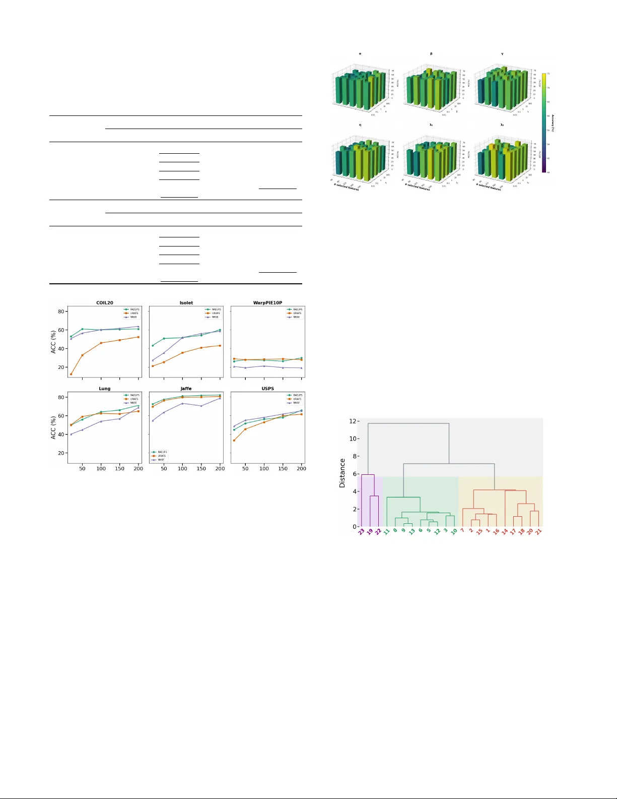
Unsupervised Feature Selection via Rob ust Autoencoder and Adapti v e Graph Learning 1 st Feng Y u, 2 nd MD Saifur R. Mazumder , 3 rd Y ing Su Department of Mathematical Sciences The University of T exas at El P aso , T exas, USA { fyu, mmazumder , ysu2 } @utep.edu 4 th Oscar Contreras V elasco Department of Sociology University of California, Davis , California, USA ocontrerasvel@ucda vis.edu Abstract —Effective feature selection is essential for high- dimensional data analysis and machine learning. Unsupervised feature selection (UFS) aims to simultaneously cluster data and identify the most discriminative featur es. Most existing UFS methods linearly project features into a pseudo-label space f or clustering, but they suffer from two critical limitations: (1) an oversimplified linear mapping that fails to captur e complex feature relationships, and (2) an assumption of uniform cluster distributions, ignoring outliers pr evalent in real-world data. T o address these issues, we propose the Robust A utoencoder - based Unsupervised Feature Selection (RAEUFS) model, which leverages a deep autoencoder to learn nonlinear feature rep- resentations while inherently impro ving rob ustness to outliers. W e further dev elop an efficient optimization algorithm for RAEUFS. Extensive experiments demonstrate that our method outperforms state-of-the-art UFS approaches in both clean and outlier -contaminated data settings. Keyw ords —unsupervised feature selection, autoencoder , Graph learning . I . I N T RO D U C T I O N In the era of big data, high-dimensional datasets have become increasingly common across various domains, includ- ing computer vision, bioinformatics, and multimedia analysis. While such data pro vides rich information, its high dimension- ality introduces big challenges in storage, computation, and model interpretability . T o mitigate these issues, dimensionality reduction techniques play a crucial role in preprocessing by transforming or selecting the most informativ e features while preserving essential data characteristics. T raditional methods like Principal Component Analysis (PCA) [1], Linear Discrim- inant Analysis (LD A) [2], Suf ficient Dimension Reduction [3, 4] project data into a lower -dimensional space through linear or nonlinear transformations. Howe ver , these approaches often obscure the original feature meanings, making interpretation difficult in real-world applications. Unlike transformation-based methods, unsupervised feature selection (UFS) directly selects a discriminativ e subset of features from the original data without altering its structure, thereby maintaining interpretability [5]. Ho wev er , in unsuper - vised learning settings, the search for discriminative features is done blindly , without having the class labels. Hence, UFS is considered as a much harder problem [6]. Existing UFS methods can be broadly categorized into three groups: Filter methods, which e valuate features based on statistical properties (e.g., variance, Laplacian score) without in volving learning algorithms [7, 8]; Wrapper methods, which employ search strategies (e.g., greedy algorithms, evolutionary computation) guided by a learning model’ s performance [6, 9]; Embedding-based methods, which integrate feature selection into an optimization frame work by leveraging sparsity re gu- larization, graph learning, or matrix factorization [10 – 13]. Embedding-based approaches hav e gained prominence in unsupervised feature selection (UFS) due to their ability to capture feature correlations and manifold structures while maintaining computational efficienc y [14]. Recent advances integrate adapti ve graph learning, non-negati ve matrix factor - ization, and discriminative constraints to enhance robustness. Howe ver , tw o key challenges remain unresolved in current embedding-based methods. First, most approaches rely on pseudo-labels in a supervised manner to approximate the true labels of the raw data, typically assuming a linear relationship between features and pseudo-labels. This simplification may fail to capture complex feature interactions. Second, existing UFS methods often o verlook the presence of outliers, which are common in real-world data. Although outliers may be grouped during the training, the features derived from them can introduce misleading information—contaminating the re- sults with irrelev ant patterns while obscuring the underlying data structure. T o address these two challenges, we propose a novel unsu- pervised feature selection framew ork that overcomes e xisting limitations by inte grating a Rob ust Subspace Recov ery (RSR) Autoencoder (AE) into an embedding framework. Our pro- posed algorithm, Robust Autoencoder-Unsupervised Feature Selection (RAEUFS), le verages the AE architecture to enhance performance in traditional UFS tasks. Additionally , the RSR layer in RSRAE effecti vely separates outliers from benign data, ensuring that the selected features accurately represent the entire dataset. Experimental results on benchmark datasets demonstrate that RAEUFS outperforms state-of-the-art UFS methods for the clean datasets. Notably , in the presence of out- lier contamination, our approach maintains high performance, whereas competing methods exhibit significant de gradation. The main contributions of this paper include: (1) introducing an autoencoder-based framework for feature embedding of unsupervised feature selection (UFS), which achiev es state- of-the-art performance; (2) inv estigating, for the first time, the impact of outliers in UFS, enhancing rob ustness in real- world scenarios; and (3) conducting extensiv e e xperiments on both benchmark datasets with ground truth and a real-world sociology dataset without ground truth, demonstrating that our proposed method, RAEUFS, effecti vely selects features and provides practical guidance for real-life applications. W e or ganize our paper as follo ws: Section II contains the literature re view . In Section III, we present RAE-RM, our robust feature selection model that combines a robust autoencoder frame work with latent space clustering of local geometric structures. The details of our algorithm, RAEUFS, for solving RAE-RM are pro vided in Section IV. Section V presents experimental results comparing RAEUFS with other methods. Finally , conclusions are drawn in Section VI. I I . R E L A T E D W O R K S Recent years have witnessed significant progress in un- supervised feature selection (UFS) through embedding-based methods. A foundational contribution is the Spectral Feature Selection (SPEC) framework [15], which unifies supervised and unsupervised feature selection by measuring feature rel- ev ance using pairwise instance similarities. Building on this, Multi-Cluster Feature Selection (MCFS) [16] employs spectral embedding to preserve data structure by optimizing feature weights in a low-dimensional space. Despite their ef fectiveness, spectral clustering-based ap- proaches face two key limitations. First, the discrete opti- mization of the cluster indicator matrix is NP-hard, often yielding solutions with mixed signs and poor sparsity . Sec- ond, an overemphasis on local data structures may lead to ov erfitting. T o address these issues, relaxation techniques are commonly adopted, where the discrete label matrix is replaced by a continuous pseudo-label matrix. This relax ed formulation preserves orthogonality by constraining the solution to the Stiefel manifold [10 – 12], enabling simultaneous learning of local and global discriminati ve structures. Moreo ver , clustering performance heavily depends on the quality of the similarity matrix and suboptimal similarity learning can degrade re- sults. Recent methods mitigate this by adapti vely learning the similarity matrix, optimizing local connectivity for improv ed clustering [17, 18]. While most UFS methods rely on linear relationships, a few explore non-linear mappings. For instance, [12] replaces linear spectral analysis with neural networks. Howe ver , autoencoders (AEs) remain widely adopted due to their strong representation learning capabilities. By compressing input features into a lo w- dimensional space and reconstructing the original data, AEs hav e demonstrated effecti veness in UFS [19, 20]. T o enhance robustness, anomaly detection can be inte grated to filter outliers before feature selection. Traditional methods like Principal Component Analysis (PCA) are sensitiv e to outliers and often fail in corrupted data scenarios. In contrast, Robust Subspace Recov ery (RSR) provides a more resilient framew ork [21 – 23]. The Rob ust Autoencoder [24] further improv es anomaly detection by utilizing the AEs. Recent advances combine AEs with RSR layers [25], where normal data points are mapped close to their original positions while anomalies are pushed away . Despite their strengths, existing methods often employ au- toencoders in a simplistic manner , neglecting robustness con- siderations that may compromise feature selection accuracy . T o bridge this gap, we propose integrating a rob ust AE framework into embedded UFS, enhancing both feature selection and outlier resilience. I I I . M E T H O D O L O G Y In this section, we first propose our rob ust autoencoder re- gression model (RAE-RM) in Section III-A and introduce the adaptiv e graph clustering technique in Section III-B, then the RAE-RM based UFS approached is provided in Section III-C. A. Robust AE Re gr ession Model. Let X = [ x 1 , . . . , x N ] ⊤ ∈ R N × D be the data matrix and suppose these N samples are sampled from d classes. Let Y = [ y 1 , · · · , y N ] ⊤ ∈ { 0 , 1 } N × d be the cluster indicator matrix, where y i ∈ { 0 , 1 } d is the cluster indicator vector for x i . The scaled cluster indicator matrix F [10] is defined as F = Y ( Y T Y ) − 1 2 . Here F = [ f 1 , f 2 , · · · , f N ] ⊤ ∈ R N × d and f i is the scaled cluster indicator of x i . Thus, the linear regression model for UFS based on the scaled indicator matrix F was proposed as follo ws [10]: min F , W ∥ X ⊤ W − F ∥ 2 F , s.t. F = Y ( Y T Y ) − 1 2 . (1) The elements of scaled cluster indicator matrix F are con- strained to discrete values, making any method relying on F computationally NP-hard. An intuiti ve approach to address this challenge is to relax F from discrete values to continuous ones under the constraint F ⊤ F = I . This relaxation preserves the orthogonality property of F , in which case the matrix F is then referred to as the pseudo-label matrix . T o model the nonlinear relation between F and the data, we incorporate a frame work of rob ust subspace recov ery autoencoder (RSR-AE) into (1) and propose RSR-AE based regression model (RAE-RM) as: min F , W , E , A ∥ ˜ Z − F ∥ 2 F , s.t. F ⊤ F = I , (2) where ˜ Z = ZA = E ( X ⊤ W ) A ∈ R N × d represents the output of the RSR layer , which follows the encoder . The encoder , E : R p → R q , maps a d -dimensional data point to a p -dimensional latent code. The RSR layer is a linear transformation A ∈ R q × d that further reduces the dimension to d . The idea behind this frame work is to embed the indicator matrix within the latent layer, rather than in the input data space, as done in the basic UFS linear regression model (1). As demonstrated in [25], the RSR layer effecti vely separates outliers from inliers, accomplishing the UFS task while si- multaneously enhancing robustness against outliers. It is worth noting that the proposed model (2) dif fers from existing AE- based UFS methods [19, 20, 26] in two ke y aspects: (1) these methods do not incorporate the pseudo-label matrix, which is typically beneficial for UFS tasks; and (2) they do not account for robustness in their design. B. Local geometric data structur e. The basic RAE-RM (2) is performed in the Euclidean space and fails to capture the local geometrical structure of the data, which is crucial for discriminativ e analysis [27]. Therefore, we cluster ˜ Z based on its local geometric structure, where ˜ Z contains the information from the original data X . The reasons for choosing to cluster ˜ Z instead of directly clustering X are twofold: first, ˜ Z is filtered by an RSR layer that can separate out the outliers, while X may contain outliers that could ne gativ ely af fect the clustering performance; second, ˜ Z represents the data in a lo wer-dimensional space, which reduces computational complexity while preserving the essential structure of the data. T o this end, we assume the pseudo label matrix F preserves the cluster structure of ˜ Z , i.e. the labels f i and f j are similar if their corresponding codes, ˜ z i and ˜ z j , are close to each other . W e denote the similarity of ˜ z i and ˜ z j by s ij and define the affinity graph S = [ s ij ] . The matrix S contains the local geometric structure for all codes and can be used to control the total scaled distances for the pseudo labels, J ( F ) = P i,j s ij ∥ f i − f j ∥ 2 . A useful property of J ( F ) is that it can be rewritten as [11]: min F 1 2 X i,j s ij ∥ f i − f j ∥ 2 = T r( F ⊤ L S F ) , where L S = D − S is the Laplacian matrix and D = diag( d 1 , . . . , d N ) is the degree matrix with d i = P N k =1 s ik . The function J ( F ) depends on the affinity graph S , while a common choice is Gaussian kernel [15, 28, 29]. That is, s ij = exp  −∥ ˜ z i − ˜ z j ∥ 2 /σ 2  , ∀ ˜ z i ∈ N k ( ˜ z j ) or ˜ z j ∈ N k ( ˜ z i ) , where N k ( ˜ z ) denotes the set of k -nearest neighbors of ˜ z . Howe ver , constructing S in this manner introduces two challenges. First, selecting an appropriate value for the bandwidth σ is critical. Second, determining the number of nearest neighbors k is also non-tri vial. T o address these two challenges, we use the adapti ve graph construction proposed by [30], in which the in verse of the information entropy of S is utilized. Thus, we consider the follo wing adaptiv e graph component in our framew ork: min F , S T r( F ⊤ L S F ) + β N X i,j =1 ( s ij log s ij ) , s.t. F ⊤ F = I . (3) C. RAE-RM based unsupervised featur e selection. The proposed RAE-RM (2) in section III-A utilizes the framew ork of the RSR-AE. W e first specify the details of its settings. Consider the input data { x i } N i =1 ⊂ R D , and denote its data matrix by X = [ x 1 , . . . , x N ] ⊤ ∈ R N × D . Let W ∈ R D × p be the coef ficient matrix and x s i := W ⊤ x i ∈ R p represent the transformed data point with p selected features. The encoder E is a neural network (NN) that maps each transformed data point to its latent code z i = E ( W ⊤ x ( t ) ) ∈ R q . The RSR layer is a linear transformation A ∈ R p × d that reduces the dimension to d and the output of RSR is ˜ z i = A ⊤ z i ∈ R d . The decoder D is a NN that maps ˜ z i to ˜ x i in the original ambient space R D . The forward maps in a compact form using the corresponding data matrices is giv en as follows: X s = X ⊤ W ∈ R N × p , Z = E ( X s ) ∈ R N × q , ˜ Z = ZA ∈ R N × d , ˜ X = D ( ˜ Z ) ∈ R N × D . In RSR-AE, the following two loss functions are considered: ℓ p 1 AE ( E , A , D ; W ) = N X i =1 ∥ x i − ˜ x i ∥ p 1 2 , (4) ℓ p 2 RS R ( A ) = λ 1 N X i =1    z i − AA ⊤ z i    p 2 2 + λ 2 ∥ A ⊤ A − I d ∥ 2 F . (5) T o enhance the robustness of the AE, we set p 1 = p 2 = 1 in (4) and (5), adopting the least absolute deviations formulation for both reconstruction and RSR. Combining the RAE-RM of (2) and the adaptiv e graph component (3), we propose the RAE-RM based unsupervised feature selection model as follows: min θ , φ , A , W , F , S ℓ 1 AE + ℓ 1 RS R + α ∥ W ∥ 2 , 1 + η ∥ ˜ Z − F ∥ 2 F + γ  T r( F ⊤ L S F ) + β N X i,j =1 s ij log s ij  s.t. F ⊤ F = I . (6) where θ , φ denote the parameters of encoder and decoder , ℓ 1 AE , ℓ 1 RS R are giv en by (4) and (5) respecti vely with p 1 = p 2 = 1 , L S is the Laplacian matrix. Here, ℓ 2 , 1 -norm regular- ization term on W is imposed to ensure W sparse in ro ws. Remark 1: The dimensionality of RAE-RM is determined by the network architectures of the encoder and decoder and certain constraints exist in specific components: • The output dimension d of ˜ Z is constrained to d ≥ c + 1 , where c is the number of clusters. This constraint ensures: (a) Cluster separation : the latent space becomes insuf fi- cient to distinguish all clusters when d < c (b) Outlier handling : The additional dimension ( +1 ) provides a dedicated subspace for outlier identification and isolation. • The encoder output dimension q must satisfy q ≥ d , ensuring the RSR layer can effecti vely serve as a bot- tleneck layer that can preserve the necessary information for cluster separation. I V . O P T I M I Z A T I O N P RO C E D U R E The proposed minimization problem (6) inv olves multi- ple variables, for which the alternating minimization (AM) method [31 – 33] (a.k.a block coordinate minimization) is particularly well-suited. Each iteration of the AM approach consists of sequential updates, where one v ariable is op- timized while keeping the others fixed. Our proposed al- gorithm solving (6), called Robust AE Unsupervised Fea- ture Selection (RAEUFS), updates the variables in the se- quence E , D , A , W , F , S and consists of two main compo- nents: (a) Iterative backpropagation of the two loss terms ℓ 1 AE + α ∥ W ∥ 2 , 1 and ℓ 1 RS R to update the RSR autoencoder parameters ( E , D , A , W ); (b) Updates for S and F , where S has an analytical solution while F can be obtained through a simple computational routine. The detailed optimization procedures for parameters E , D , A , W and F , S are presented in Sections IV -A and IV -B respectiv ely , with the complete RAEUFS algorithm summa- rized in Algorithm 2. Fig. 1. Overview of the RAEUFS algorithm A. Updating Autoencoder . When all other parameters ( A , W , F , S ) are fixed, updating the parameters of the AE at the k -th iteration reduces to the following optimization problem: min θ , φ ℓ 1 AE ( E , A ( k − 1) , D ; W ( k − 1) ) + η ∥ ˜ Z − F ( k − 1) ∥ F , (7) which is the standard autoencoder loss function. W e compute the gradients of the object in (7) with respect to θ , φ via backpropagation. The choice of optimization method depends on the dataset size: for small datasets, we apply gradient descent (GD), while for larger datasets, we use stochastic gradient descent (SGD) or Adam [34]. Similarly , the update for A , W are obtained by solving the following subproblems: arg min A λ 1 N X i =1    z ( k ) i − AA ⊤ z ( k ) i    2 + λ 2 ∥ A ⊤ A − I d ∥ 2 F , (8) arg min W N X i =1    x i − D ( A ( k ) , ⊤ E ( W ⊤ x i ))    2 + α ∥ W ∥ 2 , 1 , (9) and we backpropagate the loss functions to obtain the gradients and forward with GD or Adam. B. Updating F , S . The subproblem for solving S have closed-form solutions, whereas that for F can be addressed with a straightforw ard routine. Below , we first present the updates for F : min F ⊤ F = I η ∥ ˜ Z − F ∥ 2 F + γ T r( F ⊤ L S ( k − 1) F ) := ℓ F ( F ) . (10) Notice that the loss in (10) can be rewritten as ℓ F ( F ) = T r( F ⊤ ( η I + γ L S ( k − 1) ) F − 2 η F ⊤ ˜ Z ) + η ∥ ˜ Z ∥ 2 F , which implies that (10) is a quadratic optimization problem ov er the Stiefel manifold (QOSM). Such problems have been extensi vely studied in manifold optimization literature such as [35, 36]. T o solve (10), we employ the Generalized Power Iteration (GPI) method [37], an efficient approach for QOSM. GPI provides numerical stability and con verges in fe w iterations. The implementation details are provided in algorithm 1. Algorithm 1 GPI( ˜ Z , S ): routine for solving F 1: Input: The matrix L S ∈ R N × N , the matrix ˜ Z ∈ R N × d and regularization parameter γ , η . 2: Initialize: F (0) satisfying ( F (0) ) ⊤ F (0) = I d and ξ such that ˜ C = ξ I N − ( I N + γ η L S ) is positiv e definite. 3: for t = 1 to T do 4: M ( t ) ← 2 ˜ CF ( t − 1) + 2 ˜ Z 5: [ U , S , V ] ← RandomizedPCA ( M ( t ) ) [38] 6: Update F ( t ) ← U d V ⊤ where U d is the matrix consist- ing of the first d columns of U . 7: end for 8: Output: The pseudo label matrix F ( T ) . When all parameters except S are fixed, minimizing o ver S in (6) reduces to S ( k ) = arg min S ∈ R N × N N X i,j =1 ( ∥ f i − f j ∥ 2 2 s ij + 2 β s ij log s ij ) , s.t. N X j =1 s ij = 1 , s ij ≥ 0 , (11) which is true beacuse of the identity , T r( F ⊤ L S F ) = 1 2 P N i,j =1 ∥ f i − f j ∥ 2 2 s ij . The Lagrangian function of (11) is then giv en by ℓ S ( S ; Φ , Π) = N X i,j =1 ( ∥ f i − f j ∥ 2 2 s ij + 2 β s ij log s ij ) + N X i =1 ϕ i ( N X ij =1 s ij − 1) − N X ij =1 π ij s ij , where Φ = { ϕ i | i ∈ [ N ] } and Π = { π ij | i, j ∈ [ N ] } are the Lagrangian multipliers. The Karush–Kuhn–T ucker (KKT) conditions of ℓ S ( S ; Φ , Π) yield the follo wing equations      ∥ f i − f j ∥ 2 2 + 2 β (1 + log s ij ) + ϕ i − π ij = 0 , ∀ i, j ∈ [ N ] s ij ≥ 0 , π ij ≥ 0 , π ij s ij = 0 , ∀ i, j ∈ [ N ] P N ij =1 s ij = 1 , ∀ i ∈ [ N ] Its solution is giv en by that for ∀ i, j ∈ [ N ] , s ij = exp  − ∥ f i − f j ∥ 2 2 2 β . N X k =1 exp  − ∥ f i − f k ∥ 2 2 2 β  . (12) V . E X P E R I M E N T S In this section, we conduct extensiv e experiments to e valuate the performance of the proposed RAEUFS for feature selection in clustering tasks. The experiments consist of two main Algorithm 2 RAEUFS 1: Input: Data matrix: X ∈ R N × D , architecture of E : R p → R q and D : R d → R D with d = c + 1 , number of selected features: p , number of clusters: c , parameters: λ 1 , λ 2 , α, β . 2: Initialization: Random matrices W (0) ∈ R D × p , A ∈ R q × d , initial parameters of E , D . 3: for k = 1 to K do 4: Backpropagate (7) w .r .t. θ , φ . Update θ ( k ) , φ ( k ) . 5: Backpropagate (8) w .r .t. A . Update A ( k ) . 6: Backpropagate (9) w .r .t. W . Update W ( k ) . 7: Update F ( k ) = GPI ( ˜ Z ( k ) , S ( k − 1) ) where ˜ Z ( k ) = E ( X ⊤ W ( k ) ) A ( k ) and GPI is provided by algorithm 1 8: Update S ( k ) by (12) 9: end for 10: Output: W eight matrix, W ( K ) ∈ R D × p . parts: datasets with ground truth labels and one real world application dataset without ground truth information. A. Datasets with Gr ound T ruth Datasets. W e e valuate our method on six publicly a vailable datasets, their descriptions are pro vided in T able I. Moreov er, to assess the robustness of our algorithm, we synthetically generate outliers for each dataset by sampling from N (0 , I D ) and incorporate them into the training process. T ABLE I D E SC R I P TI O N O F T H E D A TAS E T S . Dataset Observations Features Clusters lung [39] 203 3,312 5 Jaffe [40] 213 676 10 Isolet [41] 1,560 617 26 COIL20 [42] 1,440 1,024 20 W arpPIE10P [43] 210 2,420 10 USPS [44] 9,298 256 10 Compared Methods. W e e valuate RAEUFS against two state- of-the-art UFS methods: Generalized Uncorrelated Re gression with Adapti ve Graph (URAFS) [30] and Neural Networks with Self-Expression (NNSE) [12]. After employing the methods, k -means [45] will be applied to the reduced feature data X s with repeating 100 times. Additionally , we include a baseline where k -means is applied directly to the original data without any feature selection. Parameter Settings. T o determine the optimal parameters ( α , β , γ , η , λ 1 , λ 2 ), we perform a grid search ov er the values { 10 − 2 , 10 − 1 , 1 , 10 } and best results are recorded. Evaluation Metrics. T o comprehensively e valuate perfor- mance, we use two complementary metrics: clustering accu- racy (A CC) and normalized mutual information (NMI) [46]. Both metrics assess clustering quality , with higher values indicating better performance. Since A CC and NMI capture different aspects of clustering effecti veness, their combined use enables a more thorough ev aluation of the clustering performance. For datasets containing corrupted examples, we restrict our ev aluation to only the clean data samples. Results. The comparisons of RAEUFS, URAFS, NNSE as well as the vanilla k -means for the clean and outlier- contaminated datasets are reported in T able II and T able III. The results in T able II indicate that the proposed methods RAEUFS outperforms URAFS and NNSE. The two exceptions are COIL20 in terms of A CC and USPS in terms of NMI, in which the accuracy of RAEUFS is v ery close to NNSE. T able III sho ws that e ven the datasets are contaminated with 30% outliers during the training, RAEUFS is able to identify the outliers and achie ves similar clustering performance com- pared to the clean datasets, while other algorithms degenerate the performance. The only exception is WarpPIE10P dataset that NNSE has the highest accurac y but its accuracy is much lower than RAEUFS in the clean datasets. T ABLE II C O MPA R IS O N O F R A E U FS , U R AF S , A N D N N S E W I TH 2 0 0 S E L EC T E D F E A T UR E S F O R C L E A N D A TA S ET . M E A N A N D S TAN DA R D D E V I A T IO N S ( I N PAR E N T HE S E S ) O F A CC A N D N M I A R E R E P O RTE D OV E R 1 0 0 R E PE T I T IO N S . T H E B E S T P E R FO R M AN C E A CR O SS T H E A L GO R I T HM S F O R E AC H D A TA S ET I S B O L D U N DE R L I NE D . Dataset Accuracy (A CC) (%) Baseline RAEUFS URAFS NNSE lung 66.50 (0.10) 71.08 (0.02) 64.88 (2.68) 68.72 (0.36) Jaffe 82.26 (0.07) 82.25 (0.00) 80.77 (0.90) 78.72 (0.08) Isolet 57.47 (0.03) 60.09 (0.01) 43.12 (1.21) 58.61 (0.01) COIL20 62.04 (0.03) 61.02 (0.00) 52.40 (1.59) 63.82 (0.01) WarpPIE10P 28.25 (0.02) 29.82 (0.03) 28.03 (0.61) 19.08 (0.03) USPS 57.28 (0.02) 65.78 (0.01) 61.55 (1.17) 65.24 (0.36) Dataset Normalized Mutual Information (NMI) (%) Baseline RAEUFS URAFS NNSE lung 56.64 (0.06) 59.26 (0.02) 55.40 (2.48) 57.12 (0.27) Jaffe 88.32 (0.03) 88.01 (0.01) 87.01 (0.61) 79.32 (0.13) Isolet 73.45 (0.02) 75.34 (0.01) 60.75 (1.04) 72.61 (0.00) COIL20 76.35 (0.01) 75.88 (0.01) 70.47 (1.33) 75.52 (0.02) WarpPIE10P 29.80 (0.03) 33.23 (0.01) 29.24 (1.04) 10.58 (0.01) USPS 55.80 (0.02) 61.12 (0.01) 58.08 (0.84) 61.50 (0.50) Moreov er, Fig. 2 graphically illustrates the model’ s stability and performance across the different number of selected features. On e very dataset, RAEUFS is applied along with the other 2 methods with dif ferent number of selected features (20, 50, 100, 150, 200) and record their clustering A CC scores. RAEUFS consistently achiev ed higher or matched with the highest ACC scores, indicating that it identifies more rele vant features that contribute meaningfully to clustering. Parameter sensitivity . W e additionally conduct a sensitiv- ity analysis on lung to assess how sensitive RAEUFS is to its hyperparameters. A grid search of the parameters ( α, β , γ , η , λ 1 , λ 2 ) × # selected features is performed and the results of A CC are presented in Fig. 3. Although the parameters vary logarithmically (base 10), the corresponding accuracy fluctuates irre gularly . This suggests that determining optimal parameters for a new dataset remains challenging without comprehensiv e experimental v alidation. T ABLE III C O MPA R IS O N O F R A E U FS , U R AF S , A N D N N S E W I TH 2 0 0 S E L EC T E D F E A T UR E S F O R D A TA SE T W I TH 3 0 % O U T L IE R S . M E A N A N D S TA ND AR D D E VI ATI O N S ( I N PAR E N T HE S E S ) O F A CC A N D N M I A R E R E PO RT E D OV E R 1 0 0 R E P E TI T I O NS . T H E B E S T P E R FO R M AN C E A CR O SS T H E A L GO R I T HM S F O R E A CH DAT A S E T I S B O LD U N DE R L I NE D . Dataset Accuracy (A CC) (%) Baseline RAEUFS URAFS NNSE lung 69.46 (2.96) 63.71 (2.84) 62.98 (2.64) 58.60 (0.61) jaffe 34.74 (7.18) 89.76 (0.86) 81.80 (1.00) 72.57 (0.53) Isolet 30.44 (5.28) 61.95 (1.09) 50.62 (2.49) 42.34 (0.13) COIL20 42.22 (6.37) 66.85 (0.99) 57.94 (0.85) 60.67 (0.25) WarpPIE10P 14.05 (2.05) 28.64 (0.96) 28.03 (0.67) 30.19 (0.19) USPS 58.27 (0.05) 64.56 (0.00) 60.81 (1.05) 63.59 (0.00) Dataset Normalized Mutual Information (NMI) (%) Baseline RAEUFS URAFS NNSE lung 4.80 (14.39) 57.12 (1.72) 53.84 (2.23) 49.11 (0.61) jaffe 55.69 (8.52) 91.28 (0.61) 87.81 (0.61) 76.21 (0.36) Isolet 63.58 (5.22) 75.99 (0.85) 67.56 (1.48) 60.46 (0.09) COIL20 65.35 (4.19) 78.20 (0.74) 72.96 (0.51) 73.60 (0.17) WarpPIE10P 4.33 (3.37) 30.59 (1.66) 28.21 (1.09) 31.49 (0.33) USPS 57.33 (0.03) 60.45 (0.00) 57.73 (0.94) 60.19 (0.00) Fig. 2. Performance of RAEUFS, URAFS and NNSE vs # selected features. B. Dataset without Gr ound T ruth: Migration Study acr oss U.S.-Me xico bor der . T o demonstrate the practical applicability of RAEUFS to complex real-world data, we ev aluated the method on a dataset in volving Mexican undocumented migration across the U.S.-Mexico border . The dataset stems from a survey on migration along Mexico’ s northern border (EMIF Norte) [47], and consists of surve y-based individual-le vel responses ( n = 3 , 706 ) capturing self-reported risks experienced during border crossings (e.g., abandonment, extreme temperatures, assault, etc). The primary objectiv e was to capture latent structures that dif ferentiate risk profiles across multiple cities, each with varying degrees of risk exposure. Notably , the dataset represents multiple challenges: heterogeneous feature types, measurement error , nonlinearity in feature interactions, and structural outliers. These characteristics make the dataset an ideal stress test for the robustness properties of RAEUFS. Fig. 3. ACC sensitivity of α, β , γ , η , λ 1 , λ 2 on lung . W e hypothesize that Robust Autoencoder-based Unsupervised Feature Selection (RAEUFS) can reduce the dimensionality of the EMIF Norte dataset without compromising the clustering performance. Specifically , we hypothesize that by selecting the most informati ve features, our algorithm will achie ve similar or improv ed clustering results compared to using the full set of features. The unsupervised analysis was performed on nine risk factors, grouped by city of crossing. During preprocessing, we aggregated the dataset by city , computed the av erage risk values for each city , and applied robust-scaler normalization. Hierarchical clustering using all nine features is then applied (Fig. 4), which lead to three distinct clusters. Howe ver , k - means found 2 clusters as optimal based on Silhouette scores. Fig. 4. Dendrogram of the cities based on linkage distance. T able IV demonstrates the results of k -means and Hierar - chical clustering after selecting the features from our proposed method. Using all 9 features for k =2, the hierarchical and k - means clustering achie ved silhouette scores of 0 . 51 and 0 . 57 , respectiv ely . This is our baseline score and we can see that by using only 4 features (selected by the proposed RAEUFS algorithm) we achiev ed the same result as our baseline for the hierarchical clustering. Howe ver , the highest clustering performance was achiev ed with 5 features, indicating that the algorithm successfully identified the most important fea- tures, leading to improved or comparable clustering results (T able IV). These clustering results rev eal how unsupervised learning methods can rev eal meaningful spatial variation on T ABLE IV S I LH O U E TT E S C O R ES F O R H I ER A R C HI C A L C L U ST E R IN G ( H C) A N D k - M E A N S W I TH k = 2 A N D k = 3 B Y V A R IO U S N U M BE R S O F S EL E C T ED F E A T UR E S S E L E CT E D B Y R A E U FS . k =2 k =3 # Featur es HC k -means HC k -means 3 0.46 0.44 0.34 0.29 4 0.51 0.36 0.29 0.27 5 0.51 0.57 0.29 0.29 6 0.46 0.46 0.41 0.26 7 0.50 0.50 0.29 0.29 8 0.44 0.44 0.41 0.38 9 (all) 0.51 0.57 0.29 0.32 complex social phenomena, which supports data-informed in- tervention and sociologically grounded understanding of how risk emerges and ho w it can vary across geographical domains. V I . C O N C L U S I O N W e propose RAEUFS, a novel model for the UFS problem that integrates a Robust Subspace Recov ery Autoencoder (RSR-AE) into the adaptiv e graph learning framew ork of embedding-based UFS methods. Le veraging the rob ustness of RSR-AE, RAEUFS ef fectiv ely handles data contamination and consistently achie ves the highest accuracy and NMI compared to existing methods. At the same time, it successfully identi- fies meaningful features across both synthetic and real-world datasets. Sev eral avenues for future research include: • Explor- ing adaptations of other robust autoencoder methods to the proposed framew ork. • Extending the framework to handle high-dimensional datasets with very small sample sizes could further broaden its applicability in fields such as genomics or finance. • Exploring online or incremental versions of RAEUFS would make the method suitable for streaming data scenarios, opening opportunities in real-time analytics and dynamic en vironments. R E F E R E N C E S [1] K. Pearson, “LIII. on lines and planes of closest fit to systems of points in space, ” The London, Edinbur gh, and Dublin philosophical magazine and journal of science , vol. 2, no. 11, pp. 559–572, 1901. [2] R. A. Fisher , “The use of multiple measurements in taxonomic problems, ” Annals of eugenics , vol. 7, no. 2, pp. 179–188, 1936. [3] H.-H. Huang, F . Y u, and T . Zhang, “Robust suf ficient dimension reduction via α -distance cov ariance, ” J ournal of Nonparametric Statistics , pp. 1–16, 2024. [4] H.-H. Huang, F . Y u, K. Li, and T . Zhang, “Fr ´ echet sufficient dimension reduction for metric space-valued data via distance cov ariance, ” Journal of Computational and Graphical Statistics , no. 0, pp. 1–14, 2026. [Online]. A v ailable: https://doi.org/10.1080/10618600. 2025.2602521 [5] Y . Y ang, Y . Zhuang, and Y . Pan, “Multiple kno wledge representation for big data artificial intelligence: frame- work, applications, and case studies, ” F r ontiers of Infor- mation T echnolo gy & Electr onic Engineering , vol. 22, no. 12, pp. 1551–1558, 2021. [6] J. G. Dy and C. E. Brodley , “Feature selection for unsu- pervised learning, ” J ournal of machine learning r esearc h , vol. 5, no. Aug, pp. 845–889, 2004. [7] X. He, D. Cai, and P . Niyogi, “Laplacian score for feature selection, ” Advances in neural information processing systems , vol. 18, 2005. [8] S. T abakhi, P . Moradi, and F . Akhlaghian, “ An unsuper- vised feature selection algorithm based on ant colony optimization, ” Engineering Applications of Artificial In- telligence , v ol. 32, pp. 112–123, 2014. [9] S. Maldonado and R. W eber, “ A wrapper method for feature selection using support vector machines, ” Infor- mation Sciences , v ol. 179, no. 13, pp. 2208–2217, 2009. [10] Y . Y ang, H. Shen, F . Nie, R. Ji, and X. Zhou, “Nonneg- ativ e spectral clustering with discriminative regulariza- tion, ” in Pr oceedings of the AAAI confer ence on artificial intelligence , 2011, pp. 555–560. [11] Z. Li, Y . Y ang, J. Liu, X. Zhou, and H. Lu, “Unsupervised feature selection using nonnegati ve spectral analysis, ” in Pr oceedings of the AAAI confer ence on artificial intelligence , 2012, pp. 1026–1032. [12] M. Y ou, A. Y uan, D. He, and X. Li, “Unsupervised feature selection via neural networks and self-expression with adaptiv e graph constraint, ” P attern Recognition , vol. 135, p. 109173, 2023. [13] H.-H. Huang, F . Y u, X. Fan, and T . Zhang, “ A framework of regularized lo w-rank matrix models for regression and classification, ” Statistics and Computing , vol. 34, no. 1, p. 10, 2024. [14] X. Li, H. Zhang, R. Zhang, and F . Nie, “Discrimina- tiv e and uncorrelated feature selection with constrained spectral analysis in unsupervised learning, ” IEEE T rans- actions on Image Pr ocessing , vol. 29, pp. 2139–2149, 2019. [15] Z. Zhao and H. Liu, “Spectral feature selection for supervised and unsupervised learning, ” in Pr oceedings of the 24th international conference on Machine learning , 2007, pp. 1151–1157. [16] D. Cai, C. Zhang, and X. He, “Unsupervised feature se- lection for multi-cluster data, ” in Pr oceedings of the 16th A CM SIGKDD international conference on Knowledge discovery and data mining , 2010, pp. 333–342. [17] F . Nie, X. W ang, and H. Huang, “Clustering and pro- jected clustering with adaptiv e neighbors, ” in Proceed- ings of the 20th A CM SIGKDD international confer ence on Knowledge discovery and data mining , 2014, pp. 977– 986. [18] F . Nie, W . Zhu, and X. Li, “Unsupervised feature selec- tion with structured graph optimization, ” in Pr oceedings of the AAAI confer ence on artificial intelligence , 2016. [19] K. Han, Y . W ang, C. Zhang, C. Li, and C. Xu, “ Autoen- coder inspired unsupervised feature selection, ” in 2018 IEEE international confer ence on acoustics, speech and signal pr ocessing (ICASSP) . IEEE, 2018, pp. 2941– 2945. [20] L. Y u, Z. Zhang, X. Xie, H. Chen, and J. W ang, “Un- supervised feature selection using rbf autoencoder, ” in International Symposium on Neur al Networks . Springer , 2019, pp. 48–57. [21] G. Lerman and T . Maunu, “ An overvie w of robust subspace recovery , ” Pr oceedings of the IEEE , vol. 106, no. 8, pp. 1380–1410, 2018. [22] ——, “Fast, robust and non-conv ex subspace recovery , ” Information and Infer ence: A Journal of the IMA , vol. 7, no. 2, pp. 277–336, 2018. [23] F . Y u, T . Zhang, and G. Lerman, “ A subspace-constrained tyler’ s estimator and its applications to structure from motion, ” in Pr oceedings of the IEEE/CVF Confer ence on Computer V ision and P attern Recognition , 2024, pp. 14 575–14 584. [24] C. Zhou and R. C. P affenroth, “ Anomaly detection with robust deep autoencoders, ” in Pr oceedings of the 23rd A CM SIGKDD international conference on knowledge discovery and data mining , 2017, pp. 665–674. [25] C. Lai, D. Zou, and G. Lerman, “Robust subspace re- cov ery layer for unsupervised anomaly detection, ” in 8th International Confer ence on Learning Repr esentations (ICLR) , 2020. [26] X. W u and Q. Cheng, “Fractal autoencoders for feature selection, ” in Proceedings of the AAAI Confer ence on Artificial Intelligence , 2021, pp. 10 370–10 378. [27] J. Gui, Z. Sun, W . Jia, R. Hu, Y . Lei, and S. Ji, “Dis- criminant sparse neighborhood preserving embedding for face recognition, ” P attern Recognition , v ol. 45, no. 8, pp. 2884–2893, 2012. [28] J. Shi and J. Malik, “Normalized cuts and image seg- mentation, ” IEEE T ransactions on pattern analysis and machine intellig ence , vol. 22, no. 8, pp. 888–905, 2000. [29] Shi, “Multiclass spectral clustering, ” in Pr oceedings ninth IEEE international confer ence on computer vision . IEEE, 2003, pp. 313–319. [30] X. Li, H. Zhang, R. Zhang, Y . Liu, and F . Nie, “Gen- eralized uncorrelated regression with adaptive graph for unsupervised feature selection, ” IEEE transactions on neural networks and learning systems , vol. 30, no. 5, pp. 1587–1595, 2018. [31] D. P . Bertsekas and J. N. Tsitsiklis, P arallel and Dis- tributed Computation: Numerical Methods . USA: Prentice-Hall, Inc., 1989. [32] F . Y u, L. Shen, and G. Song, “Hyperparameter estimation for sparse bayesian learning models, ” SIAM/ASA Journal on Uncertainty Quantification , vol. 12, no. 3, pp. 759– 787, 2024. [33] S. J. Wright, “Coordinate descent algorithms, ” Mathe- matical Pr ogramming , vol. 151, no. 1, pp. 3–34, Jun. 2015. [34] D. P . Kingma and J. Ba, “ Adam: A method for stochastic optimization, ” arXiv pr eprint arXiv:1412.6980 , 2014. [35] M. Journ ´ ee, Y . Nestero v , P . Richt ´ arik, and R. Sepulchre, “Generalized po wer method for sparse principal compo- nent analysis. ” J ournal of Mac hine Learning Resear ch , vol. 11, no. 2, 2010. [36] P .-A. Absil, R. Mahony , and R. Sepulchre, “Optimization algorithms on matrix manifolds, ” in Optimization Algo- rithms on Matrix Manifolds . Princeton University Press, 2009. [37] F . Nie, R. Zhang, and X. Li, “ A generalized power iteration method for solving quadratic problem on the stiefel manifold, ” Science China Information Sciences , vol. 60, pp. 1–10, 2017. [38] V . Rokhlin, A. Szlam, and M. T ygert, “ A randomized al- gorithm for principal component analysis, ” SIAM Journal on Matrix Analysis and Applications , vol. 31, no. 3, pp. 1100–1124, 2010. [39] A. Bhattacharjee, W . G. Richards, J. Staunton, C. Li, S. Monti, P . V asa, C. Ladd, J. Beheshti, R. Bueno, M. Gillette et al. , “Classification of human lung car- cinomas by mrna expression profiling rev eals distinct adenocarcinoma subclasses, ” Pr oceedings of the National Academy of Sciences , vol. 98, no. 24, pp. 13 790–13 795, 2001. [40] M. L yons, M. Kamachi, and J. Gyoba, “The japanese female facial expression (jaffe) dataset, ” 1998. [Online]. A vailable: https://data.niaid.nih.go v/resources? id=zenodo 3451523 [41] R. Cole and M. Fanty , “Isolet, ” 1991, https://archi ve.ics. uci.edu/ml/datasets/isolet. [42] S. A. Nene, S. K. Nayar , and H. Murase, “Columbia object image library (coil-20), ” T echnical Report CUCS-005-96, T ech. Rep., 1996. [Online]. A vailable: https://www .cs.columbia.edu/CA VE/software/ softlib/coil- 20.php [43] W . W ei, Q. Y ue, K. Feng, J. Cui, and J. Liang, “Unsuper- vised dimensionality reduction based on fusing multiple clustering results, ” IEEE T ransactions on Knowledge and Data Engineering , vol. 35, no. 3, pp. 3211–3223, 2021. [44] J. J. Hull, “ A database for handwritten te xt recognition research, ” IEEE T ransactions on P attern Analysis and Machine Intelligence , vol. 16, no. 5, pp. 550–554, 1994. [45] S. Lloyd, “Least squares quantization in pcm, ” IEEE transactions on information theory , vol. 28, no. 2, pp. 129–137, 1982. [46] K. Fan, “On a theorem of weyl concerning eigen values of linear transformations I, ” Pr oceedings of the National Academy of Sciences , vol. 35, no. 11, pp. 652–655, 1949. [47] El Colegio de la Frontera Norte, “Me xican survey of migration on the northern border (EMIF norte), ” 2016–2019, accessed: 2026-02-09. [Online]. A vailable: https://www .colef.mx/emif/