Mathematical Modeling of Cancer-Bacterial Therapy: Analysis and Numerical Simulation via Physics-Informed Neural Networks

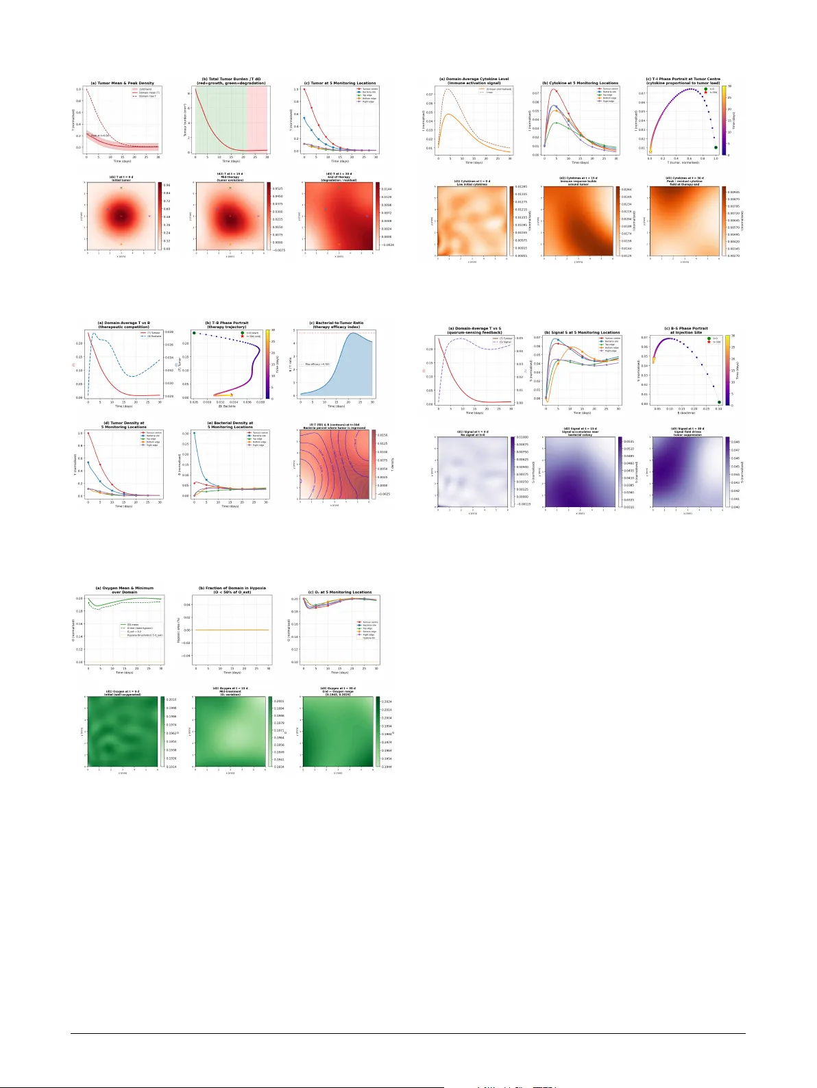
Mathematical Modeling of Cancer–Bacter ial Therapy: Anal ysis and Numerical Simulation via Phy sics-Inf ormed Neural Ne tw orks A youb Farkane a,b ,1 , Da vid Lassounon b,c,d , ∗ ,1 a TICLab, International Univ ersity of Rabat, Rabat, 11100, Mor occo b Univ ersité de Lorr aine, CNRS, CRAN, F-54000 N ancy, F rance, c Univ ersité de Lorr aine, CNRS, IECL, F-54000, N ancy, F rance, d Univ R ennes, INSA, CNRS, IRMAR-UMR 6625, F-35000, 35708, R ennes, F rance A R T I C L E I N F O Keyw ords : Phy sics-informed neural netw orks Reaction-diffusion systems T umor microenvir onment Bacterial cancer therapy Global well-posedness Numerical simulations Conv erg ence analysis A B S T R A C T Bacterial cancer therapy exploits anaerobic bacteria’ s ability to target hypoxia tumor regions, yet the interactions among tumor gro wth, bacterial colonization, oxyg en lev els, immunosuppressive cytokines, and bacterial communication remain poorly quantified. W e present a mat hematical model of fiv e coupled nonlinear reaction–diffusion equations in a two-dimensional tissue domain. W e proved the global well-posedness of t he model and identified its steady states to analyze stability . Fur thermore, a physics-inf ormed neural network (PINN) solves t he system wit hout a mesh and without req uiring extensiv e data. It pro vides con ver gence guarantees by combining residual stability and Sobolev approximation er ror bounds. This results in an o verall er ror rate of  (  −2 ln 4 (  ) +  −1∕2 ) , which depends on the network width  and t he number of collocation points  . W e conducted several numerical experiments, including predicting the tumor ’ s response to therapy . W e also per f or med a sensitivity analysis of cert ain parameters. The results suggest t hat long-ter m therapeutic efficacy ma y require the maintenance of hypo xia regions in the tumor, or using bacter ia t hat tolerate oxygen better, may be necessar y f or long-lasting tumor control. 1. Introduction 1.1. Backgr ound and Motivation of PINNs Phy sics-inf or med neural networks (PINNs) were intro- duced in w ork [ 41 ]. The y reformulate solving partial dif- f erential equations (PDEs) as minimizing a composite loss functional. This functional encodes t he governing equations, initial conditions, and boundar y conditions as soft con- straints on a neural netw ork. The approach offers t hree str uc- tural advantages ov er classical numerical me thods. Firs t, no spatial mesh is required: derivativ es are computed exactl y at an y point in t he domain via automatic differentiation through the networ k g raph [ 38 ]. Second, the method is fully unsupervised: no labeled PDE solution dat a are needed, only collocation points dra wn from the domain. Third, t he same netw ork simultaneously represents the solution at all times and all points, making temporal queries at arbitrar y resolutions tr ivial after training. These proper ties make PINNs well suited for systems of coupled, nonlinear PDEs with complex reaction terms. Classical methods often s tr uggle with suc h systems. They f ace issues like mesh stiffness, operator splitting errors, or sensitivity to time-s tep size. Howe v er, the theoretical con ver gence of PINNs applied to nonlinear systems of PDEs has remained larg ely open, wit h r igorous results confined to linear or semi-nonlinear equations [ 34 , 45 , 9 , 8 ]. The present paper addresses t his gap for a fiv e-species nonlinear reaction-diffusion system ar ising in mathematical biology . ∗ Corresponding aut hor ayoub.farkane@univ-lorraine.fr (A. Farkane); david.lassounon@univ-lorraine.fr (D. Lassounon) OR CI D (s): 1 These authors contributed equally to this wor k. 1.2. Biological Context of Bact erial Cancer Therap y In 2022 , in the w orld, 20 million new cases of cancer were diagnosed, resulting in nearl y 9.7 million deaths world- wide, according to the W or ld Healt h Organization (WHO). By 2050 , t he number of new cases is expected to reach 35 million, an increase of 77% according to [ 46 ]. As a result, cancer remains a major cause of death w orldwide. This disease results from the uncontrolled prolif eration of tumor cells. These cells escape the normal mechanisms regulating the cell cycle and apoptosis [ 19 ], thereby promoting their survival, gro wth, and resis tance to treatment. This behavior is closely linked to complex interactions with the tumor microen vironment (TME). TME is a dynamic coupled ecosystem t hat can in v olv e five main species: the tumor, bacter ia, oxy gen concentration, immunosuppressiv e cytokines, and q uor um-sensing (QS) signaling molecules. Their interactions form a netw ork of positive and negative f eedbac k loops (Figure 1 ). The tumor cells consume oxy gen, creating hypo xia niches t hat promote bacterial growth, par ticularly anaerobic bacteria. The bac- teria produce QS signals that inhibit tumor prolif eration. In addition, tumor stimulate the production of immunosuppres- sive cytokines, which, in tur n, limit bacterial prolif eration. Immunosuppressiv e Cytokines produced by tumor cells can inhibit bacter ial spread in two w ay s. On one hand, they activate local immune cells, such as macrophages and neu- trophils, which destro y bacteria. On t he other hand, t hey modify the tumor microen vironment by increasing blood perfusion or o xyg enation, making conditions less f a vorable f or the anaerobic bacter ia used in bacter ial cancer therapy (BCT). : Preprint submitted to Elsevier Page 1 of 24 T oday , BCT uses a characteristic of tumors (the pres- ence of hypo xia areas where con ventional therapies such as chemotherapy or radiotherapy are ineffectiv e). In these areas, t herapeutic anaerobic bacteria can survive [ 32 ]. For ex ample, bacteria such as Salmonella and Clostridium novyi - NT colonize t hese hypoxia areas and are activated to de- stro y tumors via their diffusible molecular signals (quor um- sensing (QS) effect) [ 21 , 1 ]. QS molecules, acyl-homoserine lactones (AHL), and autoinducer peptides (AIP) [ 18 ], ac- cumulate and are proportional to bacterial density , and are responsible for the destruction of cancer cells. Modeling this dynamic sy stem mathematically requires a nonlinear reaction-diffusion equations (PDE) to descr ibe spatial heterogeneity among different species. This approach helps us understand interactions between tumors, oxy gen, therapeutic bacteria, and tumor-induced cytokines. It also helps predict anti-cancer bacter ial activity , which is t he focus of our w ork. 1.3. Existing Mathematical Modeling Sev eral mathematical models of the tumor or immune system response and the role of h ypoxia in bacter ial ther - apy ha ve been e xtensivel y studied in recent years (see e.g. [ 33 , 32 , 43 , 27 , 36 , 2 , 21 , 14 ], and the refer ences therein). In [ 32 ], a model of anaerobic bacter ial infiltration into hypo xia areas and the effect of o xyg en on t heir growth w as studied, without accounting for the immune response or bacter ial quorum sensing. V ery recentl y , [ 14 ] proposed an ordinary differential equation model of interactions among tumors, bacteria, and chemotherapy treatment, but did not account f or the immune response or QS signaling. Further more, in [ 21 ], an ordinar y differential equation model of Salmonella - based cancer t herapies is presented. Their w ork has shown that bacterial cytoto xicity alone is insufficient to treat tumors and that activating the immune system is important for effective treatment. In their model, the spatial he terogeneity of the different species (tumors, bacteria, immune response) and also interactions wit h tumor-derived immunosuppres- sive cytokines in response to bacter ia are neglected. These often-ov erlooked biological phenomena may provide insight into t he indirect effects of anti-cancer bacteria on tumor cells and into the tumor ’ s response to their presence in its en vironment. 1.4. Deep Learning Approac hes to T umor Modeling The intersection of deep learning and mat hematical oncology has led to a rapidly growing body of research. How ev er , physics-inf ormed methods f or modeling complex, multi-species tumor microen vironment remain largel y un- explored. Early studies used PINNs in simple settings. For instance, in t his work [ 42 ] applied PINNs to find parameters in classical scalar tumor gro wth ODE models, such as the V erhulst logistic and Montroll power -la w equations. This w ork show ed robustness to experiment al noise. How ev er, these models were purely temporal and spatiall y uniform, which limited their relev ance for tumors influenced by spatial gradients of nutr ients and signaling molecules. Ot her studies ha ve focused on diagnostic applications instead of mechanistic modeling. The paper [ 25 ] dev eloped an attention-based multi-scale conv olutional neural network optimized with hybrid multi-objective CA T algorit hms, achie ving a high accuracy in classifying bone mar row cancer cells. While t his approach is highl y effective, it relies entirely on data and does no t include gov erning equations. This makes it complementary to, but fundamentally different from, ph ysics-based tumor modeling. This frame work [ 47 ] a physics-inf ormed U-Ne t f or dose prediction in intensity - modulated radiation therapy . Here, physical know ledge was included through str uctured input engineering rather t han explicit PDE residual constr aints. This show s that “ph ysics- inf or med” methods cov er a wide range of enf orcement strategies. A more rigorous PDE-constrained f ormulation w as later proposed in this paper [ 49 ]. This work combined PINNs with the Fisher–KPP reaction–diffusion eq uation. This study show ed the clinical feasibility of PINNs for single-species tumor modeling. Most recently , the wor k [ 11 ] proposed a digital twin framew ork integrated U-Net segmentation, Chan–V ese active contour refinement, and a PINN-based reaction–diffusion sol ver . Despite significant adv ances, one limitation r emains. Most tumor response models based on PINN networ ks focus on a single cell population. As a result, the y canno t account f or interactions underl ying emerging t herapies. To address this, the present work proposes and analyzes a system of five coupled nonlinear reaction-diffusion on a tissue do- main. This model descr ibes tumor response to bacter ial ther- apy , tumor oxy gen consumption, tumor -secreted immuno- suppressiv e cytokines, and quorum-sensing regulation. U n- like previous methods t hat treat the basic equations as sof t constraints wit hout f ormal guarantees, our wor k establishes the global well-posedness of the sys tem via a mass-control structure. Fur ther more, we identify three biologically rel- ev ant steady-s tates. In addition, we formally provide the suitability analy sis f or PINN appro ximation f or considered system, including approximation er ror estimates. 1.5. Contributions This paper makes the f ollo wing four contr ibutions. 1. A coupled reaction-diffusion sys tem for BCT . W e f or mulate and descr ibed system ( 8 ), coupling tu- mor density response with quorum-sensing inhibi- tion, h ypo xia-activated bacter ial gro wth (b y a inv erse Michaelis–Menten function), vascular oxy gen ex- chang e, tumor-induced immunosuppressive cytokines production in response to bacter ia (see Section 2 ). The system is the first to simult aneousl y integrate these cross-interactions. 2. W ell-posedness and steady -states analysis. Under general assumptions (H) on initial dat a and system parameters in ( 8 ), we pro ve the f ollo wing: The global exis tence, uniqueness, regular ity , and positivity of a bounded solution in an appropriate Sobole v space (see Theorem 3.1 and Proposition 3.1 , Section 3 ). W e also : Preprint submitted to Elsevier P age 2 of 24 pro vide a steady -state stability anal ysis and show that no T uring instability is induced by diffusion. Details are provided in Section 3 . 3. PINN con verg ence analy sis for our sys tem. W e es- tablish conv erg ence guarantees for t he proposed PINN applied to the system ( 8 ). Specifically , our analy sis includes: (i) a Lipschitz bound on the nonlinear op- erator (Lemma 5.1 ); (ii) a stability theorem (The- orem 5.1 ) relating approximation er ror to the net- w ork residual via energy estimates; (iii) an approxima- tion theorem (Theorem 5.2 ); and (iv) a g eneralization bound (Lemma 5.2 ) f or t he discrete loss. Finally , Theorem 5.3 combines t hese results to characterize how the method con ver ges as a function of the net- w ork arc hitecture and t he total number of collocation points. 4. Numerical simulations. W e validate t he proposed framew ork wit h numer ical simulations. W e conducted various e xperiments to anal yses t he different beha v- iors of solutions. They show t hat t he network de- scribes the complex nonlinear dynamics of the un- derl ying biological system with high precision and does not rely on synthetic or assumed parameter val- ues. Simulations confir m the expected interactions betw een t he system components, that are illustrated in Figure 1 . The rest of the ar ticle is org anized as follo w s. Section 2 f or mulates the mathematical model ( 8 ). Section 3 presents the mat hematical analysis, including the well-posedness t he- orem with a complete proof and the steady-state character i- zation. Section 4 dev elops the PINN framew ork f or the con- sidered system. Section 5 pr ov es the conv erg ence theorems f or the applied PINNs and discusses parameter calibration. Section 6 presents validation results from various numer ical experiments. Finally , Section 7 discusses limit ations and perspectives. 2. Mathematical Modeling 2.1. Ev olution of T umor Density under T reatment Mathematical modeling of tumor evolution under ther - apy (chemo therapy , immunotherapy , radiotherapy , e tc.) has been intensiv ely studied in recent y ears (see e.g. [ 10 , 5 , 23 , 22 , 35 , 31 , 28 , 29 ] and the ref erences therein) . Its value lies par ticularly in understanding the dynamic mechanisms of gro wth, resis tance, and response to treatment. The tumor response model adopted here describes the indirect action of anticancer bacter ia in tumor cells density  in the tissue via diffusible molecular signals  released by bacteria. W e consider t he follo wing reaction diffusion equation:     ( ,  ) =   Δ  ( ,  ) +    ( ,  )  1 −  ( ,  )   −    ( ,  ) −    ( ,  )  ( ,  ) in  = (0 ,  ) × Ω . (1) In equation ( 1 ),   is t he diffusion coefficient of tumor cells in tissue. The second ter m in the second member of the eq uation represents the st andard ter m descr ibing tumor cell prolif eration, characterized b y an intr insic prolif eration rate   and limited by the maximum capacity of the mi- croen vironment  [ 21 ]. The ter m −    is natural mort ality due to apoptosis or necrosis. The last term −     reflects the influence of the diffusible bacter ial signal  on the tumor population. It describe t he indirect and regulated cytoto xicity of bacteria. The higher t he concentration of  , the g reater the inhibition of tumor cells. The coefficient   is the degradation rate, and   represents the efficacy of the cytoto xic action of the diffusible bacterial signal  . The set Ω  ℝ  (  = 1 , 2 , 3 ) is open bounded represents a tissue, whose boundary  Ω is sufficientl y regular . The parameter  > 0 is the final time horizon. The quantity  ( ,  ) is the tumor density at time  ∈ (0 ,  ) and position  ∈ Ω . 2.2. Ev olution of Bacterial Density The ev olution of bacterial density  in tumor tissue is modeled b y taking into account t heir spatial diffusion, their prolif eration controlled b y o xyg en a vailability  , their nat- ural mortality , and t heir elimination by immunosuppressiv e cytokines  present in the microen vironment. W e consider the f ollo wing equation:     ( ,  ) =   Δ  ( ,  ) +    ( ,  )     +  ( ,  ) −    ( ,  ) −    ( ,  )  ( ,  ) in  . (2) The model ( 2 ) combines sev eral ke y biological processes. The quantity  ( ,  ) is t he bacter ial density at time  ∈ (0 ,  ) and position  ∈ Ω . The term   Δ  represents t he spatial diffusion of bacteria in tumor tissue. The coefficient   is the bacter ial prolif eration rate. The bacter ial g ro wth is described by the ter m      ∕(   +  ( ,  )) . In this term, the quantity   ∕(   +  ( ,  )) reflects the preference of bacteria for h ypoxia conditions. In areas with high oxy gen concentrations, there is low bacter ial g ro wth. For ex ample, therapeutic bacteria suc h as Salmonella T yphimurium or Clostridium novyi -NT germinate and prolif erate in hypo xia regions [ 50 , 44 ]. The term −    cor responds to t he natural mort ality of bacter ia with the mortality rate   . The ter m −     models bacter ial elimination by immunosuppressive cytokines  ( ,  ) with   the efficiency of t he immunosup- pressiv e response. The constant   is the diffusion coeffi- cient of bacteria, and   is the bacterial proliferation rate. The constant   is t he oxy gen inhibition constant. 2.3. Ev olution of Oxyg en Density The ev olution of oxy gen concentration, denoted as  ( ,  ) , in tissues is descr ibed by a diffusion-consumption model ( 3 ) that includes an external oxyg en [ 32 , 33 ]. This model reflects how oxy gen diffuses t hrough tissue, is consumed by tumor cells, and is replenished from t he sur rounding vascular en vironment. It provides a framew ork for representing the spatiotemporal dynamics of h ypoxia, which is a crucial f actor in tumor growth and bacter ial colonization. For the oxy gen concentration in tissues, we consider the follo wing : Preprint submitted to Elsevier P age 3 of 24 equation:     =   Δ  ( ,  ) −    ( ,  )  ( ,  ) +   (   −  ( ,  )) in  . (3) The equation ( 3 ) describes the classical processes that go v - ern o xyg en distribution within the tumor region. The term   Δ  represents the spatial diffusion of oxy gen through the tissue, where   is the diffusion coefficient that depends on the medium’ s str ucture and its porosity . The terms −     represents the consumption of oxy gen b y tumor cells. The multiplicative f orm of these terms indicates that o xy gen consumption increases with cell density and local oxyg en a vailability . The coefficients   represent the consumption rate. The term   (   −  ( ,  )) accounts f or the e x- ternal oxy gen supply from t he vascular environment. The parameter   controls the rate at whic h the local oxy- gen concentration appr oaches the ref erence value   . The value of   represents the vascular ir r igation. Including an explicit ter m representing inter nal vascular oxy gen supply is essential for accurately modeling oxyg en distr ibution within the tumor . It enables a proper balance between diffusion, cellular consumption, and t he limited contribution of blood perfusion. Without such a ter m, o xyg en gradients would be underestimated, resulting in an inadeq uate representation of hypo xia regions. 2.4. Ev olution of Immunosuppressiv e Cytokines Density The ev olution of t he density of immunosuppressiv e cytokines, denoted  ( ,  ) , in t he TME is descr ibed by a reaction-diffusion equation ( 4 ) inspired b y the w ork of [ 21 ]. The equation describes the biological process b y which tumor cells produce immunosuppressive cytokines to ev ade therapies. Secreted by tumor cells, these cytokines, such as TGF-  and IL - 10 , diffuse into sur rounding tissues to establish an immunosuppressive tumor microenvironment and naturally degrade. Tog ether , the y control inflammation, angiogenesis, and tumor cell sur vival [ 48 , 40 , 19 ]. For ex ample, cytokines IL - 10 and TNF -  activate the NF-  B signaling pathwa y , contr ibuting to inflammation and tumor progression. Their ev olution is descr ibed b y the f ollo wing equation     ( ,  ) =   Δ  ( ,  ) +    ( ,  ) −    ( ,  ) in  . (4) The model describes the distribution of tumor immunosup- pressiv e cytokines in the tissue. The term   Δ  represents the spatial diffusion of cytokines through the tissue, where   is the diffusion coefficient. The ter m    represents cytokines production b y tumor cells. This production is proportional to the local density of tumor cells and reflects tumor -induced immune activation. The term −    repre- sents the spontaneous degradation of cytokines, taking into account their half-life and elimination by consumption by other immune cells. By combining these ter ms, the model allow s for the consideration of spatial g radients and the temporal ev olution of immunosuppressive cytokines. This approach is essential for representing inhibitory effects on bacterial growth. Consequently , ( 4 ) enables t he inv estigation of immune f eedbac k on both bacteria and tumor . 2.5. Ev olution of Diffusible Bacterial Signals As explained in the first par t of the introduction, t he integration of diffusible bacter ial molecular signals repre- sented b y  acting on tumor dynamics allow s us to under- stand microbial communication, such as the quorum - sensing ([ 3 ]) on the viability of cancer cells. These signals can be acyl - homoserine lact ones (AHLs) or autoinducing peptides (AIPs) [ 18 ]. The dynamics of the diffusible bacterial signal  ( ,  ) in time and space are descr ibed by a diffusion- production-degradation model given by t he equation ( 5 ). This model show s ho w the signal diffuses through tissue, is produced by bacteria, and degrades naturall y . It show s the influence of bacterial signals of tumor viability carr ied by the ter m −     in the tumor equation ( 1 ). W e consider the f ollowing equation:     ( ,  ) =   Δ  ( ,  ) +    ( ,  ) −    ( ,  ) in  . (5) The term   Δ  refers to the spatial diffusion of the signal within the tissue, where   is t he diffusion coefficient. The term    models t he production of t he signal by bacteria, with   the production parameter . Meanwhile, the term −    accounts for the natural degradation of the signal in the tissue, where   is the degradation coefficient. The quorum - sensing mechanism play s an essential role in the collective coordination of bacteria within the tumor mi- croen vironment. Bacter ia produce and release a diffusible molecular signal into t he en vironment, the concentration of which increases with bacter ial density . When this concen- tration ex ceeds a cer tain threshold, it tr iggers t he expression of specific genes linked to vir ulence, cytotoxicity , or the production of anti-cancer enzymes. This approach makes ( 5 ) more consistent with experiment al observations of bacter ial therapies using quorum - sensing strains (e.g., Salmonella in [ 21 ] and Pseudomonas in [ 37 ]). In the literature, mathe- matical modeling of molecular signals of bacteria is of ten neglected. Their explicit inclusion highlights t heir diffuse local interactions with t he tumor . The Figure 1 presents a simplified diag ram of the main interactions betw een variables. The ar ro ws indicate the in- fluences (positiv e in green, negativ e in red) deduced from the reaction terms of the equations (without diffusion). The nodes represent onl y the variables  (tumor),  (bacteria),  (o xy gen),  (immunosuppressive cytokines),  (signal). T umor cells consume oxy gen (  →  ), which promotes hypo xia and stimulates bacter ial growth (  →  ). Bacteria produce a cytoto xic diffusible signal (  →  →  ) that inhibits tumor proliferation. The tumor also induces the production of immunosuppressive cytokines (  →  ), which ex ert an inhibitor y effect on bacter ia (  →  ), thus forming a netw ork of negative and positive f eedback loops. This inter - action describes the combined effects of hypoxia, bacter ial cytoto xicity , and the immune response on t he tumor . : Preprint submitted to Elsevier P age 4 of 24 In this paper, we will consider the follo wing initial conditions, e.g., respectivel y the initial tumor density , bac- terial density , oxig en concentration, immunosuppressive cy- tokines concentration, and the diffusible bacterial signals at initial time  = 0 and f or all  ∈ Ω :  (0 ,  ) =  0 (  ) ,  (0 ,  ) =  0 (  ) ,  (0 ,  ) =  0 (  ) ,  (0 ,  ) =  0 (  ) ,  (0 ,  ) =  0 (  ) in Ω , (6) with homogeneous Neumann boundar y conditions as f ol- low s     =     =     =     =     = 0 on Σ ∶= (0 ,  ) ×  Ω . (7) where t he vector  is the outw ard nor mal to  Ω . By combining eq uations ( 1 )-( 2 )-( 3 )-( 4 )-( 5 )-( 6 )-( 7 ), w e ob- tain the f ollowing interactive system of diffusion reaction equations:                            ( ,  ) =   Δ  ( ,  ) +    ( ,  )  1 −  ( , )   −    ( ,  ) −    ( ,  )  ( ,  ) in  ,     ( ,  ) =   Δ  ( ,  ) +    ( ,  )     +  ( , ) −    ( ,  ) −    ( ,  )  ( ,  ) in  ,     ( ,  ) =   Δ  ( ,  ) −    ( ,  )  ( ,  ) +   (   −  ( ,  )) in  ,     ( ,  ) =   Δ  ( ,  ) +    ( ,  ) −    ( ,  ) in  ,     ( ,  ) =   Δ  ( ,  ) +    ( ,  ) −    ( ,  ) in  ,     =     =     =     =     = 0 on Σ ,  (0 ,  ) =  0 (  ) ,  (0 ,  ) =  0 (  ) ,  (0 ,  ) =  0 (  ) ,  (0 ,  ) =  0 (  ) ,  (0 ,  ) =  0 (  ) in Ω . (8) The system ( 8 ) describes the simult aneous ev olution of biological variables  ,  ,  ,  ,  , representing tumor density , bacterial density , oxy gen concentration, immune cytokine concentration, and diffusible signal concentration, respec- tivel y . It formalizes the cross-f eedback loops t hat gov er n t he balance betw een tumor cell proliferation and destruction, particularly under the effect of h ypoxia and bacterial quo- rum - sensing mechanisms. This coupling provides a better representation of t he complex dynamics of the tumor mi- croen vironment under bacter ial t herapy . The mathematical analy sis of system ( 8 ) will be discussed in the follo wing section. 3. Mathematical Analysis 3.1. Existence and U niqueness of Global Classical Solutions In this section, we state and prov e the existence, unique- ness, and regularity of global classical solutions of the system ( 8 ). Before that, we make the follo wing assumptions, which we assume hold throughout t he paper . Figure 1: Simplified diagram of the main interactions variables  ,  ,  ,  ,  . General assumptions 3.1. (H) ∶ W e assume that the initial data (  0 ,  0 ,  0 ,  0 ,  0 ) =∶ 𝐔 0 ∈ (  ∞ (Ω) + ∩  1 (Ω)) 5 . The r eal diffusion coefficients   ,   ,   ,   ,   ar e non- neg ative, and the r eal prolif er ation, degr adation, and con- sumption coefficients   ,   ,   ,   ,   ,   ,   ,   ,   ,   ,   ,   ,   ,   ar e non-neg ativ e. Throughout, we denote by  a generic positive constant whose ex act value is not import ant and may v ar y from line to line. No w , we collect some kno wn definitions of a classical solu- tion of ( 8 ). For more details, w e refer the reader to [ 39 ]. Definition 3.1. The classical solution to ( 8 ) on [0 ,  ) , is a function 𝐔 ∶= (  ,  ,  ,  ,  )  ∶ [0 ,  ) × Ω → ℝ 5 suc h t hat 𝐔 ∈   [0 ,  ); (  1 (Ω)) 5  ∩(  ∞  [0 ,  −  ∗ ]×Ω  ) 5 , ∀  ∗ ∈ (0 ,  ) , and for all ,  = 1 , … ,  and all  ∈ [1 , ∞) ,   𝐔 ,    𝐔 ,      𝐔 ∈ (    (  ∗ ,  −  ∗ ) × Ω  ) 5 , and the equations in ( 37 ) ar e satisfied a.e.. Let the function F = (  1 , … ,  5 ) ∈ ℝ 5 . W e sa y t hat F is quasi-positive if it satisfies the f ollowing property: ∀  ∈ ([0 , +∞)) 5 , ∀  = 1 , … , 5 ,   (  1 , … ,   −1 , 0 ,   +1 , … ,   ) ≥ 0 , (9) where we denote  = (  1 , … ,  5 ) . W e say that F satisfies a mass-control str uctur e if there exis ts a constant  > 0 , a vector 𝐛 ∈ ℝ 5 , and a lower triangular in vertible 5 × 5 matr ix 𝐏 wit h nonnegativ e entr ies such that ∀  ∈ ([0 , +∞)) 5 , 𝐏 F(  ) ≤   1 + 5   =1    𝐛 . (10) : Preprint submitted to Elsevier P age 5 of 24 Lemma 3.1. The nonlinear ity F = (   ,   ,   ,   ,   )  fr om ( 8 ) with  = (  ,  ,  ,  ,  ) ⊺ ≥ 0 componentwise and   (  ) =     1 −    −    −     ;   (  ) =        +  −    −     ;   (  ) = −     +   (   −  );   (  ) =    −    ;   (  ) =    −    , (11) is quasi-positive and satisfies the mass-contr ol structure. Proof 1. Let  = (  ,  ,  ,  ,  ) ⊺ ≥ 0 componentwise, we have   (0 ,  ,  ,  ,  ) = 0 ≥ 0;   (  , 0 ,  ,  ,  ) = 0 ≥ 0;   (  ,  , 0 ,  ,  ) =     ≥ 0;   (  ,  ,  , 0 ,  ) =    ≥ 0;   (  ,  ,  ,  , 0) =    ≥ 0 . (12) Then, accor ding to ( 9 ) , F = (   ,   ,   ,   ,   )  is q uasi- positive. Mor eo ver , for all  = (  ,  ,  ,  ,  ) ⊺ ≥ 0 componentewise, we have   ∕(   +  ) ≤ 1 and that   (  ) +   (  ) +   (  ) +   (  ) +   (  ) ≤    +    +     +    +    ≤  (1 +  +  ) ≤  (1 +  +  +  +  +  ) , (13) implies that F = (   ,   ,   ,   ,   )  satisfies the mass- contr ol structure in the sense of ( 10 ) for 𝐏 = diag(1 , 1 , 1 , 1 , 1) and 𝐛 = (1 , 1 , 1 , 1 , 1)  . The existence of global classical solutions of ( 8 ) is given by the f ollo wing Theorem 3.1. The sy stem ( 8 ) has a unique g lobal classical solution 𝐔 = (  ,  ,  ,  ,  )  ∈ (  ∞ (  ) + ) 5 corr esponding to the initial data 𝐔 0 = (  0 ,  0 ,  0 ,  0 ,  0 )  ∈ (  ∞ (Ω) + ) 5 in the sense of Definition 3.1 . Proof 2. The global w ell-posedness of ( 8 ) is demonstr ated using a more g eneral fr amewor k presented in [ 39 , Lemma 1.1 and Theor em 3.5]. Befor e appl ying this result, we pro ve that our sy stem ( 8 ) fits w ell within this fr amew ork by sho w- ing that for all  = (  ,  ,  ,  ,  )  ≥ 0 component- wise, the nonlinear operator F(  ) satisfies [ 39 , conditions (P) and (M)] giv en by conditions ( 9 ) and ( 10 ) . Indeed, the nonlinearity F has at most polynomial and of class  1 (([0 , ∞)) 5 ; 𝐑 5 ) . By Lemma ( 3.1 ) , F satisfies the quasi- positivity condition and admits a mass-contr ol structure. Then, by [ 39 , Lemma 1.1 and Theorem 3.5], for any ini- tial data 𝐔 0 = (  0 ,  0 ,  0 ,  0 )  ∈ (  ∞ (Ω) + ) 5 , the sys- tem ( 8 ) admits a unique classical g lobal solution 𝐔 = (  ,  ,  ,  ,  )  ∈ (  ∞ (  ) + ) 5 . Since from (H) , w e ha ve more regularity on the initial data 𝐔 0 , we then demonstrate t hat the unique cor responding global classical solution satisfies the regularities given in the f ollowing Proposition 3.1. The global classical solution 𝐔 to ( 8 ) cor - r esponding to the initial data 𝐔 0 ∈ (  ∞ (Ω) + ∩  1 (Ω)) 5 satisfies 𝐔 ∈  ([0 ,  ]; (  2 (Ω)) 5 ) ∩ (  ∞ (0 ,  ;  1 (Ω))) 5 , 𝐔 ∈   2 (0 ,  ;  2 (Ω)) ∩  1 (0 ,  ;  2 (Ω))  5 . (14) suc h that for all  ∈ (0 ,  ) ,  𝐔 (  )  2 (  2 (Ω)) 5 + 2  0 ∫  0  ∇ 𝐔 (  )  2 (  2 (Ω)) 5 d  ≤   𝐔 0  2 (  2 (Ω)) 5 , (15)  ∇ 𝐔 (  )  2 (  2 (Ω)) 5 +  0 ∫  0  𝚫𝐔 (  )  2 (  2 (Ω)) 5 ) d  ≤   ∇ 𝐔 0  2 (  2 (Ω)) 5 , (16) wher e  0 ∶= min(   ,   ,   ,   ,   ) > 0 . Proof 3. Since 𝐔 0 ∈ (  ∞ (Ω) + ∩  1 (Ω)) 5  (  ∞ (Ω) + ) 5 , then according to Theorem 3.1 , t he system ( 8 ) admits a unique g lobal classical solution 𝐔 ∈ (  ∞ (  ) + ) 5 . Then, 𝐔 verifies the f ollowing abstract form of ( 8 ) .       𝐔   + 𝐀𝐔 = F( 𝐔 ) in  ,   𝐔 = 0 ℝ 5 in Σ , 𝐔 (0 ,  ) = 𝐔 0 (  ) in Ω , (17) wher e 𝐀 = − 𝐃𝚫 with 𝐃 = diag(   ,   ,   ,   ,   ) , and the nonlinearity F = (   ,   ,   ,   ,   ) define in ( 11 ) . W e have: (F( 𝐔 ) , 𝐔 ) (  2 (Ω)) 5 = ∫ Ω   ( 𝐔 )  d  + ∫ Ω   ( 𝐔 )  d  + ∫ Ω   ( 𝐔 )  d  + ∫ Ω   ( 𝐔 )  d  + ∫ Ω   ( 𝐔 )  d . (18) W e will estimat e each of the five terms of ( 18 ) . F or the first term, using the fact that  ≥ 0 since 𝐔 ≥ 0 com ponentwise, we have ∫ Ω   ( 𝐔 )  d  = ∫ Ω    2  1 −    −    2 −     2 d  ≤     2  2 (Ω) . (19) F or the second term of ( 18 ) , using 𝐔 ≥ 0 then, we hav e   ∕(   +  ) ≤ 1 and that ∫ Ω   ( 𝐔 )  d  = ∫ Ω     2     +  −    2 −     2  ≤     2  2 (Ω) . (20) : Preprint submitted to Elsevier P age 6 of 24 Similarl y to the first two estimates, using the fact that 𝐔 ≥ 0 , and Hölder’ s and Y oung’ s inequality , w e obtain ∫ Ω   ( 𝐔 )  d  = ∫ Ω  −     2 +   (    −  2 )  ≤   ∫ Ω    d  ≤   1 +    2  2 (Ω)  . (21) F or the penultimate term, applying Hölder’ s and Y oung’ s inequality, we have ∫ Ω   ( 𝐔 )  d  = ∫ Ω      −    2  d  ≤       2 (Ω)     2 (Ω) ≤      2  2 (Ω) +    2  2 (Ω)  , (22) and that ∫ Ω   ( 𝐔 )  d  = ∫ Ω      −    2  d  ≤      2  2 (Ω) +    2  2 (Ω)  . (23) By summing all estimates ( 19 ) , ( 20 ) , ( 21 ) , ( 22 ) , ( 23 ) , we obtain (F( 𝐔 ) , 𝐔 )  2 (Ω) 5 ≤   1 +  𝐔  2 (  2 (Ω)) 5  . (24) Now , taking the inner pr oduct of the fist equation of ( 17 ) by 𝐔 and using Definition 3.1 , we have    𝐔 (  ) , 𝐔 (  )  +  𝐃 ∇ 𝐔 (  ) , ∇ 𝐔 (  )  (  2 (Ω)) 5 =  F( 𝐔 (  )) , 𝐔 (  )  (  2 (Ω)) 5 , (25) wher e  ⋅ , ⋅  denotes the duality brac ke t betw een  (  1 (Ω) 5 )  ′ and (  1 (Ω)) 5 , and ( ⋅ , ⋅ ) (  2 (Ω)) 5 is the inner product in (  2 (Ω)) 5 . Setting  0 ∶= min(   ,   ,   ,   ,   ) > 0 integ rating ( 25 ) over [0 ,  ] f or all  ∈ (0 ,  ) : 1 2  𝐔 (  )  2 (  2 (Ω)) 5 − 1 2  𝐔 0  2 (  2 (Ω)) 5 +  0 ∫  0  ∇ 𝐔 (  )  2 (  2 (Ω)) 5 d  ≤ ∫  0  F( 𝐔 (  )) , 𝐔 (  )  (  2 (Ω)) 5 d  (26) Accor ding to ( 24 ) , we have for all  ∈ (0 ,  ) ∶ 1 2  𝐔 (  )  2 (  2 (Ω)) 5 − 1 2  𝐔 0  2 (  2 (Ω)) 5 +  0 ∫  0  ∇ 𝐔 (  )  2 (  2 (Ω)) 5 d  ≤  ∫  0  1 +  𝐔 (  )  2 (  2 (Ω)) 5  d . (27) F or m t he Gr önw all’ s Lemma, w e have  𝐔 (  )  2 (  2 (Ω)) 5 + 2  0 ∫  0  ∇ 𝐔 (  )  2 (  2 (Ω)) 5 d  ≤   𝐔 0  2 (  2 (Ω)) 5 . (28) Then, 𝐔 ∈  ∞ (0 ,  ; (  2 (Ω)) 5 ) ∩ (  2 (0 ,  ;  1 (Ω))) 5 . Mor eov er , since 𝐃𝚫𝐔 ∈ (  2 (0 ,  ; (  1 (Ω)) ′ )) 5 (because 𝐔 ∈ (  2 (0 ,  ;  1 (Ω))) 5 ) and F( 𝐔 ) ∈ (  2 (0 ,  ; (  1 (Ω)) ′ )) 5 (arguing as in ( 24 ) with test functions in (  1 (Ω)) 5 ), then   𝐔 = 𝐃𝚫𝐔 + F( 𝐔 ) ∈ (  2 (0 ,  ; (  1 (Ω)) ′ )) 5 . Theref ore, ac- cor ding to Aubin–Lions Lemma [ 30 ], 𝐔 ∈  ([0 ,  ]; (  2 (Ω)) 5 ) . Thus, 𝐔 ∈  ([0 ,  ]; (  2 (Ω)) 5 ) ∩ (  2 (0 ,  ;  1 (Ω))) 5 . (29) F or the other r esults regularities of 𝐔 , le t us fir st estimate F( 𝐔 ) in the (  2 (Ω)) 5 norm. W e note that  F( 𝐔 )  2 (  2 (Ω)) 5 =    ( 𝐔 )  2  2 (Ω) +    ( 𝐔 )  2  2 (Ω) +    ( 𝐔 )  2  2 (Ω) +    ( 𝐔 )  2  2 (Ω) +    ( 𝐔 )  2  2 (Ω) . (30) T aking the square term by term in ( 13 ) , and integ rating ov er Ω , we have  F( 𝐔 )  2 (  2 (Ω)) 5 ≤   1 +  𝐔  2 (  2 (Ω)) 5  . (31) T aking the inner product of the fir st equation of ( 17 ) with − 𝚫𝐔 , integ rating over Ω , using ( 31 ) , Hölder’ s, and Y oung’ s inequality, we obtain f or all  > 0 : 1 2 d d   ∇ 𝐔  2 (  2 (Ω)) 5 +  0  𝚫𝐔  2 (  2 (Ω)) 5 ≤  F( 𝐔 )  (  2 (Ω)) 5  𝚫𝐔  (  2 (Ω)) 5 ≤    F( 𝐔 )  2 (  2 (Ω)) 5 +   𝚫𝐔  2 (  2 (Ω)) 5 ≤    1 +  𝐔  2 (  2 (Ω)) 5  +   𝚫𝐔  2 (  2 (Ω)) 5 . (32) By choosing  =  0 2 , and using a nonlinear Gr önwall Lemma, we have for all  ∈ (0 ,  ∗ ) :  ∇ 𝐔 (  )  2 (  2 (Ω)) 5 +  0 ∫  0  𝚫𝐔 (  )  2 (  2 (Ω)) 5 d  ≤   ∇ 𝐔 0  2 (  2 (Ω)) 5 . (33) This implies that 𝐔 ∈ (  ∞ (0 ,  ;  1 (Ω)) ∩  2 (0 ,  ;  2 (Ω))) 5 . (34) Accor ding to ( 31 ) , and since 𝐔 ∈ (  2 (  )) 5 , we hav e F( 𝐔 ) ∈ (  2 (  )) 5 . Mor eo ver , since 𝐔 ∈ (  2 (0 ,  ;  2 (Ω))) 5 , it follow s that 𝐃𝚫𝐔 ∈ (  2 (  )) 5 . Therefor e, we obtain   𝐔 = 𝐃𝚫𝐔 + F( 𝐔 ) ∈ (  2 (  )) 5 . (35) Ther efor e, the estimates and r egularity r esults ( 29 ) , ( 34 ) , ( 35 ) , ( 28 ) , and ( 33 ) complete the pr oof of Pr oposition 3.1 . : Preprint submitted to Elsevier P age 7 of 24 Remar k 3.1. W e used a homogeneous N eumann boundar y condition for all v ariables  ,  ,  ,  ,  in ( 7 ) to maintain a clear mathematical and numerical framew ork for analyzing syst em ( 8 ) . In our future wor k , we may consider other boundar y conditions for some of the five variables, as in [ 28 , 29 ], where a nonlinear term is used at the boundar y to model tumor invasion into other or g ans. 3.2. Nondimensionalization of the sy stem In order to introduce dimensionless variables, we con- sider t he follo wing rescalings:   =    ;  x = x  ;  =      ;   =   ;   =   ∗ ;   =    ;   =   ∗ ;   =   ∗ ;  ∗ =      ;  ∗ =    ∗   . (36) By replacing , ,  ,  ,  ,  ,  obt ained by ( 36 ) in ( 8 ), w e ha ve in  Ω =∶ Ω∕  , t he follo wing dimensionless system (for simplicity , the tildes are omitted):                     = Δ  +  (1 −  ) −  0  −  0   ,    =   Δ  +  0    +  −  0  −  0   ,    =   Δ  −  0   +  0 (1 −  ) ,    =   Δ  +  −  0  ,    =   Δ  +  −  0  ,    =    =    =    =    = 0 on Σ ,  (0 ,  ) =  0 (  );  (0 ,  ) =  0 (  );  (0 ,  ) =  0 (  );  (0 ,  ) =  0 (  );  (0 ,  ) =  0 (  ) , (37) where t he dimensionless parameters are given by   =     ;   =     ;   =     ;   =     ;  0 =     ;  0 =     ;  0 =     ;  0 =     ;  0 =     ;  0 =    ∗   ;  0 =    ∗   ;  0 =      ;  0 =     ;  =     . (38) 3.3. Homogeneous s teady states analy sis In t his subsection, w e consider the system ( 37 ) omitting spatial dependence in order to study spatiall y homogeneous steady states. The Theorem 3.1 guaranteed that the solution of system ( 37 ) is positive and bounded. The f ollowing propo- sition give the spatially homogeneous steady states and t heir positivity conditions Proposition 3.2. The system ( 37 ) admits three spatially ho- mog eneous s tationar y states giv en by: •  0 = (0 , 0 , 1 , 0 , 0) corresponding to the tumor -free equilibrium. • If  0 < 1 , then   =  1 −  0 , 0 ,  0  0 +  0 (1 −  0 ) , 1 −  0  0 , 0  corr esponds t o the bacteria-fr ee tumor equilibrium. • If the f ollowing conditions  0 < 1;  0 <  0  1 +  ;  0 +  0  0 (1 −  0 ) >  0  (  0 +  0 (1 −  0 ))  (  0 +  0 (1 −  0 )) +  0 , (39) ar e me t, then  ∗ =    ,  0  0 (1 −  0 −   ) ,  0  0 +  0   ,    0 , 1  0 (1 −  0 −   )  corr esponds to the coexist ence equilibrium, where   ∈]0 , 1 −  0 [ satisfies the quadratic equation:  0  (  0 +  0   )  (  0 +  0   ) +  0 =  0 +  0  0   . (40) Proof 4. A spatially homog eneous steady state (   ,   ,  ,   ,   ) of ( 37 ) satisfies:    =    =    =    =    = 0 , Δ  = Δ  = Δ  = Δ  = Δ  = 0 . Thus, the st eady st ates are solutions of the system          0 =   (1 −   ) −  0   −  0     , 0 =  0     +   −  0   −  0     , 0 = −  0     +  0 (1 −   ) , 0 =   −  0   , 0 =   −  0   . (41) F r om the last two equations w e obtain   =    0 ,   =    0 . (42) Mor eov er , in the third equation of ( 41 ) the oxy g en density satisfies   =  0  0 +  0   . (43) Substituting ( 42 ) into the first two equations of ( 41 ) giv es 0 =    1 −   −  0 −  0    0  , (44) 0 =     0   +   −  0 −  0    0  . (45) W e now identify the possible st eady s tates. : Preprint submitted to Elsevier P age 8 of 24 ∙ T umor -fr ee equilibrium. If   =   = 0 , then according to ( 42 )   = 0 ,   = 0 and fr om ( 43 ) w e obtain   = 1 . Thus the tumor -free equilibrium is  0 = (0 , 0 , 1 , 0 , 0) . ∙ Bacteria-free tumor equilibrium. If   = 0 , then   = 0 and ( 44 ) - ( 45 ) becomes   (1 −   −  0 ) = 0 . Hence   > 0 , if  0 < 1 i.e.,   <   , we obtain   = 1 −  0 . F r om ( 42 ) and ( 43 ) , the v ariables   ,   ar e   = 1 −  0  0 ,   =  0  0 +  0 (1 −  0 ) . Ther efor e the tumor equilibrium without bacteria is   =  1 −  0 , 0 ,  0  0 +  0 (1 −  0 ) , 1 −  0  0 , 0  . ∙ Coexistence equilibrium. If   > 0 and   > 0 , fr om ( 44 ) , ( 42 ) and ( 43 ) we obtain   = 1 −  0 −  0    0 ;   =    0 ;   =    0 ;   =  0  0 +  0   . (46) Then, according to ( 45 ) the coexistence equilibrium satisfy the condition  0   +   =  0 +  0    0 . (47) W e now det er mine the positive coexistence steady state  ∗ = (   ,   ,  ,   ,   ) . F or that, suppose that conditions ( 39 ) ar e met. Substituting   =  0 ∕(  0 +  0   ) in equation ( 47 ) we have an quadr atic equation for   :  0  (  0 +  0   )  (  0 +  0   ) +  0 =  0 +  0  0   . (48) Let define t he function  in ℝ + suc h that  (  ) =  0  (  0 +  0  )  (  0 +  0  ) +  0 −  0 −  0  0  . Equation ( 48 ) can be r ewritten as  (   ) = 0 . (49) W e have  (0) =  0  1 +  −  0 ,  (1 −  0 ) =  0  (  0 +  0 (1 −  0 ))  (  0 +  0 (1 −  0 )) +  0 −  0 −  0  0 (1 −  0 ) . (50) Accor ding to conditions ( 39 ) , w e obtain  (0) > 0 and  (1 −  0 ) < 0 and since  is continuous on ℝ + , then the equation ( 49 ) has at least one solution   in ]0 , 1 −  0 [ . Once the existence of   ∈]0 , 1 −  0 [ is es tablished, then fr om ( 46 ) and according to ( 39 ) ag ain w e have   =  0  0 (1 −  0 −   ) > 0;   =    0 ;   = 1  0 (1 −  0 −   );   =  0  0 +  0   . (51) Ther efor e, we have the exist ence of the coexist ence equilib- rium  ∗ = (   ,   ,  ,   ,   ) where   ∈]0 , 1 −  0 [ satisfies ( 48 ) and   ,  ,   ,   are given by ( 51 ) , which ter minates the proof of Proposition 3.2 . 3.4. Stability analy sis of the steady st ates W e analyze t he stability of the homogeneous system derived from ( 37 ). This allows us to establish the conditions of the s tability of equilibr ium states, t aking into account t he f or mation of spatial patter ns. Let  = (   ,   ,  ,   ,   ) be a homogeneous equilibrium descr ibed Proposition 3.2 . W e study the local stability of t he homogeneous equilibr ium states  . Let 𝐔 = (  ,  ,  ,  ,  )  solution of ( 37 ). The system ( 37 ) can be rewritten in the abstr act f orm ( 17 ) with   𝐔 = 𝐃𝚫𝐔 + F( 𝐔 ) , where 𝐃 = diag(1 ,   ,   ,   ,   ) and F( 𝐔 ) the reaction operator ter ms in ( 37 ). No w , by linearize the sys tem around  by writing 𝐔 =  + , we hav e t hat t he per turbation term  satisfies    = 𝐃𝚫𝐮 +  (  ) , (52) where  (  ) is the Jacobian matr ix of F evaluated at  defined by  (  ) =  1 − 2   −  0 −  0  0 0 0 −  0   0  0   +   −  0 −  0   −  0    (  +   ) 2 −  0   0 −  0   0 −  0   −  0 0 0 1 0 0 −  0 0 0 1 0 0 −  0  . Due to Neumann ’ s boundary conditions in ( 37 ), the f ollow - ing Laplacian eigen v alue problem −Δ   =     admits a sequence of positiv e eig env alues (   )  =1 , ⋯ , 5 such that  1 = 0 <   f or all  = 2 , ⋯ , 5 which correspond respectiv ely to scalar eigenfunctions (   )  =1 , ⋯ , 5 . W e assume t hat the perturbation  as in the f orm  ( ,  ) =     (  )   (  ) , where the function   ∈  1 ([0 ,  ]; ℝ 5 ) , and substituting into the linearized equation ( 52 ) gives f or all  = 1 , ⋯ , 5 ∶ d   d  =   (  ) −   𝐃    . (53) Theref ore the stability of the equilibrium  is determined by the eig en values of the matr ices   ,  = 1 , ⋯ , 5 such t hat:   =  (  ) −   𝐃 . (54) W e ha ve the f ollo wing r esults : Preprint submitted to Elsevier P age 9 of 24 Proposition 3.3. • The tumor-fr ee equilibrium  0 = (0 , 0 , 1 , 0 , 0) is locally asympt otically stable if  0 > 1 and  0   + 1 <  0 . (55) • The tumor equilibrium   =  1 −  0 , 0 ,  0  0 +  0 (1 −  0 ) , 1 −  0  0 , 0  exists for  0 < 1 and is locally asymptotically stable if  0   +   <  0 +  0 1 −  0  0 , (56) wher e   =  0  0 +  0 (1 −  0 ) . • The coexistence equilibrium  ∗ = (   ,   ,  ,   ,   ) is locally asympt otically stable if ther e exists. Proof 5. • The tumor -free equilibrium  0 = (0 , 0 , 1 , 0 , 0) . Assume that  0 > 1 , and  0   + 1 <  0 . Evaluating   at  0  = 1 , ⋯ , 5 gives   (  0 ) =  1 −  0 −   0 0 0 0 0  0   +1 −  0 −     0 0 0 −  0 0 −  0 −     0 0 1 0 0 −  0 −     0 0 1 0 0 −  0 −      . Since   ≥ 0 and coefficients   ,   ,   ,   ≥ 0 , then all r eal eig envalues of   (  0 ) ar e neg ative. Hence  0 is locally asympt otically stable. • Bacteria-free tumor equilibrium:   = (1 −  0 , 0 ,  0  0 +  0 (1 −  0 ) , 1 −  0  0 , 0) . Assume that  0 < 1 and the condition ( 56 ) is satisfied. F or  = 1 , ⋯ , 5 the eigen values of   (   ) are given by  1 = −(1 −  0 ) −   ≤ 0 ,  2 =  0   +   −  0 −  0   −     ≤ 0 ,  3 = −  0 (1 −  0 ) −  0 −     ≤ 0 ,  4 = −  0 −     ≤ 0 ,  5 = −  0 −     ≤ 0 . Then, all real eig env alues of   (   ) are neg ative. Ther efor e   is locally asymptotically stable under the condition ( 56 ) . • The coexistence equilibrium  ∗ = (   ,   ,  ,   ,   ) satisfying ( 51 ) and ( 48 ) . Af ter calculating all nonzero coefficients of  (  ∗ ) , the matrix   (  ∗ ) is:   (  ∗ ) =     −   −   0 0 0 −  0   0 −     −  0    (  +   ) 2 −  0   0 −  0   0 −  0   −  0 −     0 0 1 0 0 −  0 −     0 0 1 0 0 −  0 −         . The eigenv alues of the matrix   (  ∗ ) are given by  1 = −   −   ≤ 0 ,  2 = −  0 −     ≤ 0 ,  3 = −  0 −     ≤ 0 ,  4 = −  0   −  0 −     ≤ 0 ,  5 = −     ≤ 0 . (57) Then, all spatial per turbations decay exponentially and the coexis tence equilibrium  ∗ is locally asymp- totically stable. F or  = 0 , we have  5 = 0 , and thus  ∗ is non-hyperbolic for the homog eneous system in space, but r emains stable with r espect to spatial perturbations. Remar k 3.2. The diffusion intr oduces the terms −   𝐃 , whic h shift the eig env alues to war d the negativ e half-plane. Then, for  > 0 , no eigen values of   (  ∗ ) become positive, and diffusion canno t destabilize the equilibrium. Theref or e, no T uring instability is induced b y diffusion [ 35 ]. 4. PINNs Approximation Solving system ( 8 ) numer ically poses specific challenges that motivate the use of PINNs. Classical mesh-based meth- ods such as finite elements or finite differences require a spatial mesh whose resolution must be adapted to the three orders-of-magnitude gap betw een the f astest diffusion coefficient, and must handle the stiff vascular ex c hange term t hrough costly implicit time-stepping. Bey ond these technical difficulties, the fiv e nonlinearly coupled equations require either operator-splitting which introduces splitting er rors or the assembl y of large block Jacobians at each Ne wton s tep. PINNs [ 41 ] circum vent all t hree issues simultaneousl y: spatial and temporal coordinates are treated as continu- ous inputs, der ivativ es are computed ex actly by automatic differentiation with no truncatio n er ror , and all five equa- tions are enf orced simult aneously as soft constraints on a single trainable loss, with no mesh and no time-stepping stability condition to satisfy . The mathematical analy sis of Section 3.1 guarantees the exis tence and uniq ueness of a solution 𝐔 = (  ,  ,  ,  ,  )  ∈   ([0 ,  ];  2 (Ω)) ∩  2 (0 ,  ;  1 (Ω))  5 to system ( 8 ). To compute this solution numerically , we employ a PINNs [ 41 , 13 , 12 ], an approach that embeds the governing equations, initial conditions, and boundary conditions directly into the loss functional of a deep neural network, thereby transf orming the PDE problem into an unconstrained optimisation problem ov er the networ k weights. In this context recently many paper hav e focused on the using the deep leanrning methods for solving the he The fundament al idea is to seek an approximation  𝐔  ∶  ⟶ ℝ 5 , (58) realised by a single feedf orward ne twork   ∶ ℝ 3 → ℝ 5 with trainable parame ters  , such that  𝐔  ≈ 𝐔 in t he sense : Preprint submitted to Elsevier P age 10 of 24 of minimising a physics-based loss defined belo w . Because no labelled simulation data are required, the method is fully unsuper vised : t he only super vision comes from t he physical la ws encoded in ( 8 ). 4.1. Netw or k Architectur e The neural network   maps the spatio-temporal co- ordinate ( , ,  ) ∈ Ω × (0 ,  ) to the five-dimensional state vect or:   ( , ,  ) =    ,   ,  ,   ,    ( , ,  ) . (59) W e employ a fully connected Multi-La yer Perceptron (MLP) architecture consisting of  lay ers. The architecture com- prises an input lay er, sever al hidden la yers of unif or m width, and an output la yer cor responding to the state variables. The hidden-lay er activation is the hyperbolic tangent  (  ) = t anh(  ) . This choice is motiv ated b y its infinite differentia- bility , which ensures that the high-order par tial der iv atives required f or t he differential operators in system ( 8 ) can be computed accurately through automatic differentiation with- out inter polation errors. Let 𝐡 (0) = ( , ,  )  ; the forw ard pass reads 𝐡 ( 𝓁 ) =    ( 𝓁 ) 𝐡 ( 𝓁 −1) + 𝐛 ( 𝓁 )  , 𝓁 = 1 , … ,  − 1 , (60)   ( , ,  ) =  (  ) 𝐡 (  −1) + 𝐛 (  ) , (61) where {  ( 𝓁 ) , 𝐛 ( 𝓁 ) }  𝓁 =1 are the weight matr ices and bias vec- tors collected in  . W eights are initialised using the Xavier unif or m scheme, which keeps t he variance of activations stable across la yers and accelerates con v ergence [ 16 ]. 4.2. Derivativ e Computation via A utomatic Differentiation For every scalar network output   ∈ {   ,   ,  ,   ,   } , all partial der iv atives required by the residual operators of ( 8 ) are computed e xactly by rev erse-mode aut omatic differenti- ation (AD) [ 38 ], implemented in PyT orch. Concretely : • First-order derivativ es     ,     ,     : one backw ard pass t hrough the computation g raph. • Laplacian Δ   =     +     : a second backw ard pass applied to     and     , respectivel y . This av oids any finite-difference tr uncation er ror and re- mov es the mesh dependency from der ivativ e computation entirely . 4.3. Collocation P oint Sampling Three disjoint sets of collocation points are drawn to enf orce sy stem ( 8 ): Interior (PDE) points  pde : A set of  pde collocation points (   ,   ,   ) ∈  sampled uniformly , with (   ,   ) ∼ 𝐔 (Ω) and   ∼ 𝐔 (0 ,  ) . Initial condition points  ic : A set of  ic points (   ,   , 0) ∈ Ω × {0} dra wn uniformly ov er Ω . Boundary points  bc : A set of  bc points (   ,   ,   ) ∈  Ω × (0 ,  ) , dra wn unif or ml y on eac h of the four sides of  Ω , with   ∼ 𝐔 (0 ,  ) . In practice t he union  =  pde ∪  ic ∪  bc is par titioned into training (60%), validation (20%), and test (20%) subsets. 4.4. Composite Loss Functional The total loss to be minimised o v er  is  (  ) =  pde  pde (  ) +  ic  ic (  ) +  bc  bc (  ) , (62) where the weights are set to  pde ,  ic ,  bc . These weights pla y an impor tant role in t he conv erg ence of the PINNs loss. In par ticular, choosing  ic >  pde ensures t hat the netw ork remains consistent with the prescribed initial conditions (see ( 6 )). This weighting ensures t hat the lear ned spatio- temporal solution follo ws the given initial profiles. If t he initial-condition term is assigned too little weight, t he model ma y focus on reducing the PDE residual, which can cause it to conv erg e to the trivial solution 𝐔 ≡ 0 instead of the intended physical solution. 1. PDE Residual Loss: The five residual operators   ,   ,   ,   ,   are obtained by substituting the netw ork outputs into the left-hand sides of ( 8 ):   =     −   Δ   −      1 −     +     +       ; (63a)   =     −   Δ   −         +   +     +       ; (63b)   =     −   Δ   +       −   (  vas −   ); (63c)   =     −   Δ   −     +     ; (63d)   =     −   Δ   −  (  )    +     . (63e) Setting  ∶= {  ,  ,  ,  ,  } , the PDE loss is then the mean-squared residual o v er  pde :  pde (  ) = 1  pde  pde   =1   ∈     (   ,   ,   ;  )  2 . (64) 2. Initial Condition Loss: The initial condition loss enf orces ( 6 ) at  = 0 :  ic (  ) = 1  ic  ic   =1   ∈     (   ,   , 0;  ) −  0 (   ,   )  2 , (65) where  0 denotes the initial profile of each species given in ( 6 ). Concretely , we consider the follo wing initial conditions:  0 ( ,  ) = exp  −  ( ,  ) − 𝐱   2 2  2   , (66a) : Preprint submitted to Elsevier P age 11 of 24  0 ( ,  ) = 0 . 3 exp  −  ( ,  ) − 𝐱   2 2  2   , (66b)  0 ( ,  ) =  vas ,  0 ( ,  ) = 0 . 01 ,  0 ( ,  ) = 0 , (66c) where, the tumor centre is 𝐱  = (  ∕2 ,  ∕2) , 𝐱  = (0 . 3 , 0 . 6  ) is t he bacterial injection site,   =  ∕5 and   =  ∕8 are the spatial spreads, and  = 6 mm. The Gaussian profile ( 66a ) initialises a localised tumour seed at 10% of t he car rying capacity  , while ( 66b ) places a v ery small bacterial inoculum (  0   0 ) at an off-centre position, simulating a targe ted injection a wa y from the tumour cor e. 3. Boundary Condition Loss The homogeneous Neumann conditions ( 7 ) are en- f orced by penalising the squared gradient nor m on  bc :  bc (  ) = 1  bc  bc   =1   ∈     ∇ ( , )   (   ,   ,   ;  )    2 . (67) Note that the gradient ∇ ( , )   is again computed e x- actly via AD, so no approximation of the outward normal 𝐧 is needed. Proposition 4.1 (Consis tency of the PINN loss). Let  ∗ be such that  (  ∗ ) = 0 . Then the networ k   ∗ satisfies the residuals   ≡ 0 for all  at every collocation point in  pde , r eproduces the initial data at every point in  ic , and satisfies the zero-flux condition at ever y point in  bc . More details about the numer ical parameters and implemen- tation de tails are descr ibed in the section 6 . In the next section, we pro vide a r igorous conv er gence analy sis of the proposed PINN framew ork and establish er ror estimates for the me thod. 5. Con ver gence Analy sis of the PINN Appro ximation Let 𝐔 = (  ,  ,  ,  ,  )  be the unique classical so- lution of system ( 8 ) cor responding to the initial data 𝐔 0 (guaranteed b y Theorem 3.1 -Proposition 3.1 ), and let  𝐔  = (   ,   ,  ,   ,   )  be the PINN approximation produced by the netw ork   ∶ ℝ 3 → ℝ 5 after minimizing the composite loss ( 62 ). Define the total appr oximation error as 𝐞 ( , 𝐱 ) = 𝐔 ( , 𝐱 ) −  𝐔  ( , 𝐱 ) , ( , 𝐱 ) ∈ . (68) The total error admits the three-w a y decomposition:  𝐞   ∞ (0 , ;(  2 (Ω)) 5 ) ≤  appr ox (  )      (I) approximation +  gen (  )    (II) generalization +  opt (  ∗ )    (III) optimisation , (69) where: Algorithm 1 PINN Training for System ( 8 ) Req uire: Collocation sets  pde ,  ic ,  bc ; w eights  pde ,  ic ,  bc ; A patience  ; the maximum epochs  . Ensure: Best-v alidation-loss weights  ∗ . 1: Initialise  with Xavier unif or m distr ibution. 2:  ∗ ← +∞ ;  ← 0 . 3: for  = 1 , … ,  do 4: Sample mini-batch of size 512 from each collocation set. 5: Compute  (  ) via forw ard pass + AD (Sec. 4.2 ). 6: Update  ←  −  ∇   (  ) via Adam. 7: Evaluate  val on t he held-out v alidation se t. 8: if  val <  ∗ then 9:  ∗ ←  val ;  ∗ ←  ;  ← 0 . 10: else 11:  ←  + 1 . 12: end if 13: if  ≥  then br eak  Early stopping 14: end if 15: Adjust  via ReduceLR OnPlateau scheduler . 16: end for 17: return  ∗ . (I) Appro ximation error : the best-ac hiev able error of a depth-  , width-  network in approximating t he tr ue solution 𝐔 ∈ (  2 (0 ,  ;  1 (Ω))) 5 . (II) Generalization error : t he discrepancy betw een the empirical (Monte Carlo) loss e valuated on  pde ,  ic ,  bc collocation points and t he continuous  2 - residuals ov er  , Ω , and Σ . (III) Optimisation error : the gap between the loss achie ved by the Adam algorithm af ter  epochs and t he global minimum of the loss landscape. Item (III) depends on the specific optimization trajector y and is not addressed here; w e pro vide upper bounds f or (I) and (II), and we der ive a conditional stability estimate show - ing that if (I) and (II) are small, t hen  𝐞   ∞ (0 , ;(  2 (Ω)) 5 ) is small. W e begin by defining t he continuous residual functionals associated wit h t he PINN appro ximation 𝐔  . 5.1. Continuous Residual F unctionals Define the continuous (tr ue) residuals associated with the PINN appro ximation  𝐔  :  pde (  ) = ∫  0 ∫ Ω   ∈       (  𝐔  ; , 𝐱 )    2 d 𝐱 d , (70)  ic (  ) = ∫ Ω   ∈       ( 𝐱 , 0;  ) −  0 ( 𝐱 )    2 d 𝐱 , (71)  bc (  ) = ∫  0 ∫  Ω   ∈     ∇ 𝐱   ( 𝐱 ,  ;  ) ⋅ 𝐧    2 d  d , (72) : Preprint submitted to Elsevier P age 12 of 24 T able 1 The numerical simulation parameters of the system ( 8 ) Equation Description Symb ol Value Unit All T umor cell motility   0 . 01 mm 2 da y −1 Bacterial diffusivit y   0 . 1 mm 2 da y −1 Oxygen diffusivit y   1 . 0 mm 2 da y −1 Cytokine diffusivit y   0 . 5 mm 2 da y −1 AHL signal diffusivity   0 . 3 mm 2 da y −1 (1) T umo r  Proliferation rate   0 . 3 da y −1 Ca rrying capacit y  1 . 0 normalised Ap optosis rate   0 . 05 da y −1 Signal supp ression coeff.   0 . 2 da y −1 (2) Bacteria  Gro wth/clearance rate   0 . 5 da y −1 O 2 half-saturation   0 . 1 no rmalised Natural death rate   0 . 1 da y −1 Immune clea rance efficiency   0 . 3 da y −1 (3) Oxygen  T umor O 2 consumption   0 . 2 da y −1 V ascular exchange rate   0 . 5 da y −1 Baseline O 2 level  ext 0 . 2 no rmalised (4) Cytokines  T umor-derived production   0 . 1 da y −1 Cytokine deca y rate   0 . 2 da y −1 (5) Signal  p ro duction rate   0 . 4 da y −1 degradation rate   0 . 3 da y −1 where   are the five residual operators defined in ( 63 ). Let  (  ) =  pde  pde +  ic  ic +  bc  bc denote t he total continuous loss. 5.2. Lipschitz Continuity of the Nonlinear Operator In this section, w e first establish t hat the nonlinear func- tion F ∶ ℝ 5 → ℝ 5 defined in ( 11 ) is locall y Lipschitz. Lemma 5.1 (Lipschitz bound on F ). Ther e exists a con- stant   > 0 such that  F( 𝐔 ) − F(  𝐔  )  (  2 (Ω)) 5 ≤  F  𝐞  (  2 (Ω)) 5 , a.e.  ∈ (0 ,  ) . (73) Proof 6. Theorem 3.1 guar antees 𝐔 ∈ (  ∞ (  ) + ) 5 when- ever 𝐔 0 ∈ (  1 (Ω) ∩ (  ∞ (Ω) + ) 5 . F or the networ k ap- pr oximation  𝐔  , boundedness is enforced by the bounded weight initialisation and the t anh activation (whose output is alw ays in (−1 , 1) ). Then, there exists constants  such that  𝐔  (  ∞ (  )) 5 ≤  , and   𝐔   (  ∞ (  )) 5 ≤  . Now , recall fr om ( 11 ) the five components of F :   ( 𝐔 ) =     1 −    −    −     ;   ( 𝐔 ) =        +  −    −     ;   ( 𝐔 ) = −     +   (   −  );   ( 𝐔 ) =    −    ;   ( 𝐔 ) =    −    . W e bound   ( 𝐔 ) −   (  𝐔  ) in  2 (Ω) with  =  ,  ,  ,  ,  . Let   =  −   for each component. T erm   :   ( 𝐔 ) −   (  𝐔  ) = (   −   )   −    (  +   )   −   (   −     ) . Since    ≤  ,     ≤  and using the assum ption (H) , the first term is bounded by        2 (Ω) . F or the second term, using the fact that   −     =    +     , and    ≤  ,     ≤  :    −       2 (Ω) ≤        2 (Ω) +        2 (Ω) . Hence    ( 𝐔 ) −   (  𝐔  )   2 (Ω) ≤         2 (Ω) +      2 (Ω)  . (74) : Preprint submitted to Elsevier P age 13 of 24 T erm   : F or the fr actional term, w e hav e      +  −       +   = (  2  +   )    −       (   +  )(   +   ) . Since  ,   ≥ 0 , w e have (   +  )(   +   ) ≥  2  , and using     ≤  ,     ≤  and assumption ( H) , we obtain:           +  −       +         2 (Ω) ≤   (      2 (Ω) +      2 (Ω) ) . F or the res t of terms, w e have −    +     −     +       = −     −   (    +     ) . Using     ≤  ,     ≤  and assumption ( H) , w e obtain:    ( 𝐔 ) −   (  𝐔  )   2 (Ω) ≤         2 (Ω) +      2 (Ω) +      2 (Ω)  . (75) T erms   ,   ,   : Using    ,    ,    ≤  , we have similarl y obtained as the pr evious estimates, the f ollowing:    ( 𝐔 ) −   (  𝐔  )   2 (Ω) ≤         2 (Ω) +      2 (Ω) +      2 (Ω)  ; (76)    ( 𝐔 ) −   (  𝐔  )   2 (Ω) ≤         2 (Ω) +      2 (Ω)  ; (77)    ( 𝐔 ) −   (  𝐔  )   2 (Ω) ≤         2 (Ω) +      2 (Ω)  . (78) Summing estimat es ( 74 ) - ( 78 ) with 𝐞 = (   ,   ,   ,   ,   )  , and setting   =   , completes the pr oof of Lemma 5.1 . 5.2.1. Conditional Stability: Error Controlled by Residuals The central result of t his section sho w s that small PDE, IC, and BC residuals impl y a small approximation er ror . Theorem 5.1 (Conditional Stability). Let the assumptions of Theorem 3.1 hold and let  𝐔  ∈ (  2 (0 ,  ;  1 (Ω)) ∩  1 (0 ,  ; (  1 (Ω)) ′ )) 5 be any networ k appro ximation. Define the total residual  (  ) =  pde (  ) +  ic (  ) +  bc (  ) . Then there exists a constant  =  (  ,  ,   ,  0 ) > 0 , independent of  , suc h that sup  ∈[0 , ]  𝐞 (  )  2 (  2 (Ω)) 5 +  0 ∫  0  ∇ 𝐞 (  )  2 (  2 (Ω)) 5 d  ≤   (  ) . (79) Proof 7. Step 1 — Error equation. Since 𝐔 satisfies (10) exactly and  𝐔  satisfies it with residual 𝐑  = (   ,   ,   ,   ,   )  , subtr acting gives for a.e.  ∈ (0 ,  ) :   𝐞 + 𝐀𝐞 = F( 𝐔 ) − F(  𝐔  ) − 𝐑  in , (80a)  𝐧 𝐞 = −  𝐧  𝐔  on Σ , (80b) 𝐞 (0 , ⋅ ) = 𝐔 0 −  𝐔  ( ⋅ , 0) in Ω . (80c) Step 2 — Energy identity . T ake the (  2 (Ω)) 5 inner pr oduct of ( 80a ) with 𝐞 and integr ate o ver Ω . Integ r ation by par ts, using the boundar y condition ( 80b ) , yields 1 2 d d   𝐞 (  )  2 (  2 (Ω)) 5 +  𝐃 ∇ 𝐞 , ∇ 𝐞  (  2 (Ω)) 5 =   ( 𝐔 ) −  (  𝐔  ) , 𝐞  (  2 ) 5 −  𝐑  , 𝐞  (  2 (Ω)) 5 + ∫  Ω 𝐃  𝐧  𝐔  ⋅ 𝐞 d  . (81) Step 3 — Bounding the r ight-hand side of ( 81 ) . Nonlinear ter m. By Lemma 5.1 :   ( 𝐔 ) −  (  𝐔  ) , 𝐞  (  2 (Ω)) 5 ≤    𝐞  2 (  2 (Ω)) 5 . (82) Residual ter m. By Y oung’ s inequality for all  > 0 :    ( 𝐑  , 𝐞 ) (  2 (Ω)) 5    ≤ 1 2   𝐑   2 (  2 (Ω)) 5 +  2  𝐞  2 (  2 (Ω)) 5 . (83) Boundary term. Using the trace inequality in  2 (  Ω) (see [ 6 , Theorem 1.6.6.]), and Y oung’ s inequality, we have for all  > 0 :     ∫  Ω 𝐃  𝐧  𝐔  ⋅ 𝐞 d      ≤  𝐃  ∞   𝐧  𝐔   (  2 (  Ω)) 5  𝐞  (  2 (  Ω)) 5 ≤   , Ω 2    𝐧  𝐔   2 (  2 (  Ω)) 5 +   , Ω 2    ∇ 𝐞  2 (  2 (Ω)) 5 +  −1  𝐞  2 (  2 (Ω)) 5  . (84) Step 4 — Differential inequality. Since fr om ( 17 ) , 𝐀 = − 𝐃𝚫 with 𝐃 = diag(   ,   ,   ,   ,   ) , we have ( 𝐃 ∇ 𝐞 , ∇ 𝐞 ) (  2 (Ω)) 5 ≥  0  ∇ 𝐞  2 (  2 (Ω)) 5 , wher e  0 = min(   ,   ,   ,   ,   ) . Substituting bounds ( 82 ) – ( 84 ) into ( 81 ) , and choosing  =   0 ∕2   , Ω to absorb the gr adient term: d d   𝐞  2 (  2 (Ω)) 5 +  0  ∇ 𝐞  2 (  2 ) 5 ≤ Λ  𝐞  2 (  2 (Ω)) 5 +  1  𝐑   2 (  2 (Ω)) 5 +  2   𝐧  𝐔   2 (  2 (  Ω)) 5 , (85) wher e Λ = 2   +  +   , Ω ,  1 =  −1 ,  2 =  −1   , Ω ar e constants depending only on  ,  0 , and the tr ace constant   , Ω . Step 5 — Application of Grönw all’s Lemma. Integr at- ing ( 85 ) ov er [0 ,  ] and applying Grönw all’ s Lemma:  𝐞 (  )  2 (  2 (Ω)) 5 +  0 ∫  0  ∇ 𝐞  2 (  2 (Ω)) 5 d  : Preprint submitted to Elsevier P age 14 of 24 ≤  Λ    𝐞 (0)  2 (  2 (Ω)) 5 +  1 ∫  0 ∫ Ω   ∈      2 d 𝐱 d  +  2 ∫  0 ∫  Ω   ∈    𝐧    2 d  d   . (86) Recognising  𝐞 (0)  2 (  2 ) 5 =  ic (  ); ∫       2 =  pde (  ); ∫ Σ    𝐧    2 =  bc (  ) , and taking the supremum ov er  ∈ [0 ,  ] gives ( 79 ) with  =  Λ  max(1 ,  1 ∕  ic ,  2 ∕  bc ,  1 ∕  pde ) . Remar k 5.1 (Role of the IC weight  ic ). Estimate ( 79 ) show s that the error bound is pr oportional to  (  ) , whic h in- cludes  ic  ic . A lar g e  ic for ces the optimiser to r educe  ic aggr essiv ely, thereby tightening the bound. This pro vides justification for the c hoice a higher  ic used in tr aining. 5.2.2. Neur al N etwork Approximation Capacity W e no w address the question of a neural netw ork’ s ability to approximate t he e xact solution of the pair system. The Proposition 3.1 gives the Sobolev regular ities of the solution 𝐔 of the system ( 8 ) cor responding to the initial data 𝐔 0 ∈ (  ∞ (Ω) + ∩  1 (Ω)) 5 . Precisel y , we ha v e 𝐔 ∈   2 (0 ,  ;  2 (Ω)) ∩  1 (0 ,  ;  2 (Ω))  5 =∶   2 , 1 (  )  5 . Based on well-kno wn classical results in the analysis of parabolic equations, t his is natural Sobolev regular ity of solutions to second-order parabolic systems with initial dat a  1 (Ω) . The regular ity  2 , 1 (  ) of the global solution of ( 8 ) is sufficient f or estimating conditional st ability (Theorem 5.1 ). How ev er , the approximation theorem (Theorem 5.2 ) re- quires additional regularity of the global solution (which we do not hav e wit h t he initial data in (  1 (Ω)) 5 to approxi- mate residual operators related to der ivativ es within second- order spaces. At least one additional order of differentia- bility bey ond the larg est derivativ e order  is required to appro ximate (  = 2 for ( 8 )), according to the pr inciple  ≥  + 1 using in [ 15 , Theorem 1.] and [ 9 , Theorem 5.1], where  is the maximum order of derivativ es used in the Sobolev norm. To ensure this additional regularity of the global solution, it is assumed in onl y this section that the initial data 𝐔 0 ∈ (  2 (Ω)) 5 . Using the same classical techniq ues in the proof of Proposition 3.1 , w e ha ve that the associated global solution 𝐔 of ( 8 ) satisfies 𝐔 ∈   2 (0 ,  ;  3 (Ω)) ∩  2 (0 ,  ;  2 (Ω))  5 . Theorem 5.2 (Appr oximation by t anh ne twor ks). Let the solution 𝐔 of system 8 corresponding to the initial data 𝐔 0 ∈ (  2 (Ω)) 5 satisfying 𝐔 ∈   2 (0 ,  ;  3 (Ω)) ∩  2 (0 ,  ;  2 (Ω))  5 =∶  . Then for any  > 0 , there exists a fully connected t anh netw ork 𝐍  ∶ ℝ 3 → ℝ 5 with  layer s of width  satisfying min   (  ) ≤ , (87) pr ovided that  is c hosen lar ge enough. More pr ecisely, f or the continuous loss  pde +  ic +  bc : min    pde (  ) +  ic (  ) +  bc (  )  ≤  appr ox ln 4 (  )  2  𝐔  2  , (88) wher e  𝐔  2  ∶=  𝐔  2 (  2 (0 , ;  3 (Ω))) 5 +  𝐔  2 (  2 (0 , ;  2 (Ω))) 5 , and  appr ox depends on  ,  Ω  , and the system par ameter s (   ,   ,   ,   ,   ,   ) but is independent of  and  . Proof 8. The proof combines the Sobolev appro ximation theor y for t anh netw orks established in [ 15 , Theor em 1 and Cor ollar y 2] with the structure of the residual operator s 63a - 63e . Step 1 - Component-wise appro ximation. As explained at the beginning of the subsection, the residual operat ors   defined in 63a - 63e use at most  = 2 derivatives (the Laplacian Δ repr esented by second-order spatial derivatives and   r epresent ed by a fir st-or der t emporal derivative). Ther efor e, to bound  pde in  2 (  ) , we must control the appr oximation er r or in the Sobolev norm   , 2 (  ) . T o do this, we apply a tighter appro ximation bound f or Sobolev - r egular functions (see [ 15 , Theorem 1] with  =  + 1 = 3 ) component-wise to each variable  ∈ {  ,  ,  ,  ,  } . Then, ther e exists a t anh netw ork    with width paramet er  suc h that for all 0 ≤  ≤ 2 :   −      , 2 (  ) ≤  [appr ox] , 3 , 3 Δ [t anh] , 3 , 3 (  ;   , )     3 , 2 (  ) , (89) wher e t he asympt otic equiv alence ter m Δ [t anh] , 3 , 3 (  ;  ) ∼   +  +  2   ln   1     −  , (90) with  = 3 ,  = 3 ,  = 2 , and  ∼  −1 . In our situation, the dominant asymptotic equivalence t er m is obtained for (  =  = 2) . Then the t er ms  [appr ox] 2 , 3 , 3 , Δ [t anh] 2 , 3 , 3 (  ) ar e given by Δ [t anh] 2 , 3 , 3 (  ) ∼ 16 ln 2  1    = 16 ln 2 (  )  ,  [appr ox] 2 , 3 , 3 ∼ 2 × 3 9∕2 (1 +  )  6  3  3   3 . (91) Step 2 — PDE r esidual bound. Since 𝐔 satisfies ( 8 ) , the r esidual f or each component takes the f orm   ( 𝐍  ) =     −   Δ   −    ( 𝐔 ) −   (  𝐔  )  , : Preprint submitted to Elsevier P age 15 of 24 wher e   =  −    . Then w e hav e:      2 (  ) ≤        2 (  ) +    Δ     2 (  ) +    ( 𝐔 ) −   (  𝐔  )   2 (  ) . The first tw o terms are contr olled by the  1 , 2 (  ) and  2 , 2 (  ) nor m of appro ximation error s from Step 1. The nonlinear term is bounded by the Lipschitz estimate of Lemma 5.1 :    ( 𝐔 ) −   (  𝐔  )   2 (  ) ≤    𝐞  (  2 (  )) 5 . Ther efor e:  pde (  ) = ∫    ∈      2 d 𝐱 d  ≤    ∈  2   =0   −     2  , 2 (  ) . Applying ( 89 ) f or  = 0 , 1 , 2 and using ( 90 ) , w e obt ain  pde (  ) ≤  ln 4 (  )  2   ∈     2  3 , 2 (  ) . (92) Step 3 — IC and BC terms. By t he trace Theorem, the initial condition error satisfies:  ic (  ) ≤    ∈    −     2  1 , 2 (  ) ≤  ln 2 (  )  4  𝐔  2 (  3 , 2 (  )) 5 , whic h is of higher or der than  pde . Similarly ,  bc is con- tr olled by the boundar y tr ace of  ∇      2 (  Ω) , bounded via the  2 , 2 (  ) appr oximation error . Summing the three contributions yields ( 88 ) . 5.2.3. Generalization: From Em pirical to Continuous Loss The PINN is trained by minimising the empir ical (Monte Carlo) loss  (  ) defined in ( 62 ) o v er finite collocation sets. W e now quantify ho w closely  (  ) appro ximates the tr ue continuous functional  (  ) . Let the PDE domain  = (0 ,  ) × Ω hav e measure    =   Ω  , and define the rescaled empir ical estimator   pde (  ) =     pde  pde   =1   ∈       (   ,   ;  )    2 , (93) and similarly   ic ,   bc with their respective domains. Lemma 5.2 (Monte Carlo generalization bound). Assume the residual functions   (  ;  ) ∶=    (  ;  )  2 ar e uniformly bounded: sup  ∈ ,      (  ;  )  ≤  < ∞ . Then for any  ∈ (0 , 1) , with pr obability at least 1 −  ov er the random dr aw of  pde i.i.d. uniform points in  :      pde (  ) −  pde (  )    ≤      2 ln(2∕  )  pde . (94) The same bound holds for    ic −  ic  with  ic and  Ω  , and for    bc −  bc  with  bc and  Σ  =    Ω  . Proof 9. The rescaled estimator ( 93 ) is   pde (  ) =    ⋅   , wher e   =  −1 pde    (   ;  ) is the sample mean of the bounded random variable  (  ;  ) =     (  ;  ) ∈ [0 ,  ] . The tr ue functional is  pde (  ) =    ⋅ 𝔼 [  (  ;  )] . By Hoeffd- ing’ s inequality applied to  pde i.i.d. samples fr om [0 ,  ] : ℙ       − 𝔼 [  ]    ≥   2 ln(2∕  ) 2  pde  ≤  . Multiplying by    gives ( 94 ) . Remar k 5.2 (Con verg ence r ate). The g eneralization err or decr eases as  (  −1∕2 ) with r espect to the number of col- location points, which is the standar d Monte Carlo rate. Higher -or der quasi-Monte Carlo sampling (e.g., Sobol se- quences) can impr ov e this to  ((log  )  ∕  ) (see [ 7 ]). 5.2.4. Conv ergence Result Combining the conditional stability estimate (Theo- rem 5.1 ), the approximation t heorem (Theorem 5.2 ), and the Monte Carlo generalization bound (Lemma 5.2 ), we ar r iv e at t he follo wing conv erg ence result. Theorem 5.3 (PINN Conv erg ence f or System ( 8 ) ). Let  𝐔  ∗ be the PINN appro ximation obtained by minimising   (  ) ov er the class of t anh networ ks with  layers of width  . Then f or any  ∈ (0 , 1) , with pr obability at leas t 1 −  ov er the random draw of collocation points : sup  ∈[0 , ]  𝐔 (  ) −  𝐔  ∗ (  )  2 (  2 (Ω)) 5 ≤     appr ox ln 4 (  )  2  𝐔  2  +  (  pde ,  ic ,  bc ,  )  , (95) wher e   =   (  ,  ,   ,  0 ) > 0 is the stability constant from Theor em 5.1 , independent of  , and the gener alization ter m is  =  pde      2 ln(2∕  )  pde +  ic   Ω   2 ln(2∕  )  ic +  bc   Σ   2 ln(2∕  )  bc . (96) In par ticular : : Preprint submitted to Elsevier P age 16 of 24 • As  → ∞ (wider netw ork), the appro ximation term vanishes as  (  −2 ln 4 (  )) . • As  pde ,  ic ,  bc → ∞ , the g ener alization term  → 0 at r ate  (  −1∕2 ) . • The combined err or decay s as   ln 4 (  )  2 +  −1∕2  as ,  → ∞ , (97) wher e  = min(  pde ,  ic ,  bc ) . Proof 10. F r om Theor em 5.1 w e have: sup  ∈[0 , ]  𝐞 (  )  2 (  2 (Ω)) 5 ≤    (  ∗ ) . Decompose the continuous loss:  (  ∗ ) =   (  ∗ ) −   (  ∗ )       gener alisation error +   (  ∗ )    empirical loss . Empirical loss term. Since  ∗ minimises   , and the ap- pr oximating netw ork  appr ox fr om Theor em 5.2 achiev es  (  appr ox ) ≤  appr ox  −2 ln 4 (  )  𝐔  2  :   (  ∗ ) ≤   (  appr ox ) ≤  (  appr ox ) +      (  appr ox ) −  (  appr ox )    ≤  appr ox ln 4 (  )  2  𝐔  2  +  . Gener alisation error ter m. Applying Lemma 5.1 component- wise to   (  ∗ ) −  (  ∗ ) and summing the bounds for the PDE, IC, and BC contributions gives   (  ∗ ) −   (  ∗ )  ≤  with pr obability at least 1 −  . Combining the tw o bounds yields ( 95 ) . Using the left-hand side of the estimate ( 86 ) in Theorem 5.1 , we also obt ain con ver gence in the energy norm giv en by the f ollowing Corollary 5.1. Under the same assumptions of Theorem 5.3 :  0 ∫  0  ∇ 𝐞 (  )  2 (  2 (Ω)) 5 d  ≤     appr ox ln 4 (  )  2  𝐔  2  +   . (98) Remar k 5.3 (P ositivity pr eservation). Theor em 3.1 guar - antees 𝐔 ≥ 0 component-wise for non-neg ativ e initial data. The networ k output  𝐔  does not automaticall y inherit this pr operty. Howev er , Theor em 5.3 implies that when  → ∞ we have   𝐔  ∗ − 𝐔   ∞ (0 , ;(  2 (Ω)) 5 ) → 0 , so the neg ative part norm   𝐔 −  ∗  (  2 (Ω)) 5 ≤  𝐞  (  2 (Ω)) 5 → 0 as well when  → ∞ . 6. Numerical Results This section tests the proposed PINN framew ork with thorough numerical e xperiments on the fiv e-species tumor- bacteria system ( 8 ) in a domain Ω ∈ ℝ 2 representing t he tissue. W e show that the trained netw ork effectivel y captures the spatiotempor al dynamics introduced by t he mathemati- cal analy sis in previous sections. W e also confirm the f our- phase therapy progression mentioned in the abstract: initial tumor g ro wth, hypo xia bacter ial activation, quor um-sensing mediated tumor suppression, and coexistence. For the code and other details, please ref er to our repository 1 6.1. Implementation Details The neural netw ork arc hitecture is emplo yed a full y connected feedf orward netw ork wit h architecture [3 , 64 , 64 , 64 , 64 , 5] . This architecture is comprising f our hidden la yers of 64 neurons eac h with tanh activation, and a linear output la yer producing the fiv e state v ariables  𝐔 = (   ,   ,  ,   ,   )  . The network has 21,829 trainable param- eters and processes spatio-temporal coordinates ( , ,  ) ∈ [0 , 6] × [0 , 6] × [0 , 30] as input. For the collocation points Training data consists of  pde = 10 , 000 inter ior points sampled uniformly ov er  = (0 , 30) × Ω ,  ic = 600 initial condition points at  = 0 , and  bc = 400 boundar y points on  Ω × (0 , 30) . The full dataset is par titioned 60% ,20%, 20% into training, validation, and test subsets f ollowing standard practice. Remar k 6.1. In the loss functions, we set  ic = 50 . 0 to enfor ce initial condition fidelity, while  pde = 1 . 0 and  bc = 1 . 0 . This w eighting prev ents collapse to the trivial solution 𝐔 ≡ 0 . It also makes sur e the netw ork follo ws the specified Gaussian tumor seed and bacterial inoculum. Neural network parameters are optimised b y the Adam algorit hm [ 26 ], with an initial learning rate of  0 = 10 −3 . ReduceLR OnPlateau decays this rate with a factor of 0 . 5 and patience of 1000 epochs. Overfitting can be av oided by stop- ping earl y and being patient f or  = 2000 epoc hs. The size of the mini-batc h is 512 . All calculations are car r ied out on the T esla T4 15 Go using PyTorc h 2.0. Earl y stopping wit h patience  epochs prevents ov er fitting. The full procedure is summarised in Algor ithm 1 . All parameters enter ing system ( 8 ) are calibrated from peer -revie wed experimental and computational literature. T able 1 pro vides a complete listing. 6.2. T raining The training history in Figure 2 demonstrates successful PINN optimization across all loss components. The network con ver ges to a best validation loss of  best val ≈ 1 . 2 × 10 −3 at epoch 7894, demonstrating stable optimization without ov er - fitting. The T otal composite loss decreases from ∼ 10 3 to  (10 −3 ) with training (blue) and validation (orange) cur ves tracking closely , indicating good g eneralization. Moreo ver , PDE residual loss e xhibits monotonic decay from ∼ 10 2 to 1 https://github.com/FARKANE/- T umor-Bacterial- Therapy-PINNs : Preprint submitted to Elsevier P age 17 of 24 Figure 2: T raining and validation loss evolution over 8000 ep ochs. 1 . 1 × 10 −3 , confir ming that the netw ork lear ns to satisfy the five coupled reaction-diffusion equations. Additionally , initial condition loss drops sharply in the first 2000 epochs from ∼ 10 1 to  (10 −5 ) due to the high weighting  ic = 50 . 0 , confirming strong adherence to t he prescribed Gaussian profiles. The last sub-figure represents show s t hat boundary condition loss decreases from ∼ 10 0 to  (10 −4 ) , validating enf orcement of the zero-flux Neumann conditions. The red dashed line marks t he best epoch (7894) where earl y stop- ping is triggered. 6.3. Results and Discussion Figure 3 show s the comple te spatiotemporal dynam- ics of bacter ial cancer therapy as descr ibed b y the trained PINN. This presents evolution of the five-species tumor- bacteria system o ver 30 da ys on the 6 × 6  2 tissue domain. Each row cor responds to a temporal snapshot at  ∈ {0 , 5 , 10 , 15 , 20 , 25 , 30} day s; columns sho w tumor density  (red), bacterial density  (blue), oxyg en  (green), im- munosuppressiv e cytokines  (orange), and quor um-sensing signal  (pur ple). The PINN solution was sampled at fixed spatial locations ov er time to ensure a thorough anal ysis of the e xperiments. The coordinates f or t hese locations are provided in Table 2 . The solution demonstrates f our therapeutic stages: (I) tumor g ro wth reaching  max ≈ 0 . 96 by  = 5 da ys; (II) tumor decrease to  ≈ 0 . 05 in spite of low bacterial density (  ∼ 0 . 04 – 0 . 09 ); (III) accumulation of signals (  ≈ 0 . 05 – 0 . 07 ) f acilitating ongoing tumor cells suppression; (IV) a nearly tumor -free condition (  ≈ 0 . 01 ,  ≈ 0 . 04 ) by  = 30 da ys. Oxy gen le vels s tay close to baseline (  ≈ 0 . 19 – 0 . 20 ) throughout the process, while cytokines cor respond to tumor density . The solution has four clear phases: Phase I (0-5 da ys): T umor expansion. At the beginning, the tumor variable  is at its maximum value ((  max ≈ 0 . 96)) . The bacter ia (  0 ) , introduced slightly aw a y from t he tumor center, begin to grow and mov e to w ard the tumor . Even though t he tumor consumes oxyg en rapidl y , t he oxy gen level  stays relativ ely stable near the vascular value (  vas ≈ 0 . 20) because t he vascular supply is high. Phase II (5–15 day s) : The tumor gets smaller . Even though the bacter ia load is low and the oxy gen lev els are normal, the tumor density drops shar ply from  ≈ 0 . 96 to  ≈ 0 . 05 . This is because of natural tumor cell death (    ), car r ying capacity saturation, and the start of quorum-sensing suppres- sion ( −     ). Bacter ial density lev els off at  ≈ 0 . 04 , which is the r ight amount for immune clearance (     ) to keep up wit h oxy gen-modulated growth. The QS signal starts to build up (  ≈ 0 . 05 – 0 . 07 ) and spreads from the bacterial site to the tumor center . This activates t he cytoto xic term −     ≈ −0 . 01  . Phase III (15–25 days): QS-mediated suppression. T umor density continues decreasing (  ≈ 0 . 05 → 0 . 01 ) as the stabilized signal (  ≈ 0 . 05 ) maintains suppression. Bacteria reach a plateau at  ≈ 0 . 04 in a state of quasi- equilibrium, where production ( ≈ 0 . 167  ) balances clear- ance ( ≈ 0 . 106  ). Cytokines decay proportionally to tumor (  ≈ 0 . 03 → 0 . 01 ), reducing immune pressure on residual bacteria. Phase IV (>25 days): Near-tumor -free coexistence. The system approaches a lo w-density equilibrium: (  ,  ,  ,  ,  ) ≈ (0 . 01 , 0 . 04 , 0 . 19 , 0 . 01 , 0 . 05) , which cor - responds to a near stable tumor -free equilibrium (Proposi- tion 3.2 ) rather than complete eradication. Persistent bacter ia act as a reservoir for QS signals, stopping tumors from growing back ev en when the immune system isn ’ t as strong. The Figure 4 illustrates the tumor dynamics throughout the 30-da y therapy . In panel (a), the domain-a verag ed tumor density rises to an earl y maximum before enter ing a steady , monotonic decline. At t he same time, the v ariability bands progressivel y nar row , reflecting increasing spatial unifor - mity as the tumor regresses. Panel (b) depicts t he ov erall tu- mor burden. A short-lived initial growth phase (highlighted in red) precedes an e xtended degradation per iod (shown in g reen), clearly illustrating the t herapeutic impact of t he bacterial inter vention. P anel (c) emphasizes spatial hetero- geneity . The tumor center undergoes t he most pronounced regression, whereas monitoring points near t he boundaries remain close to baseline lev els, confirming that the tumor remains confined within t he computational domain. The spatial snapshots in the bottom ro w (d1–d3) provide a visual summary of this progression. The tumor begins as a concentrated Gaussian-like core, transitions into a more diffuse intermediate configuration during therapy , and ul- timately approaches a nearly uniform low -density residual state by t he end of treatment. Figure 5 shows how tumors interact with bacteria and t he outcomes of treatments. Panel (a) illustrates t hat as t he tumor (red) decreases in size, bacteria (blue dashed) initially de- cline but then stabilize at moderate levels. This indicates that a high number of bacter ia isn’ t necessary f or effectiv eness. Panel (b) depicts the sys tem from a state of high tumor/lo w bacteria (green circle) to significant tumor shr inkage while bacteria le vels remain moderate (red st ar) ov er a period of 30 days. Panel (c) illustrates that the bacteria-to-tumor : Preprint submitted to Elsevier P age 18 of 24 Figure 3: Spatio-temporal evolution of the five-sp ecies tumor-bacteria system over 30 days. T able 2 Monito ring Prob e Lo cations in Figure 1 Symb ol Colo r Location ( ,  ) Purpose × Red (3 . 0 , 3 . 0) T umo r center-initial tumor seed location × Blue (1 . 8 , 3 . 6) Bacteria injection site, 30%  , 60%  of domain × Green (3 . 0 , 5 . 5) T op edge, Nea r-boundary monitoring point × Orange (3 . 0 , 0 . 5) Bottom edge, Near-boundary monito ring p oint × Purple (5 . 5 , 3 . 0) Right edge, Nea r-boundary monitoring point ratio peaks when t he tumor is small enough. This indicates the effectiv e treatment. Panels (d) and (e) depict spatial dynamics. The g reatest tumor reduction occurs at the center , while bacteria tend t o stay close to t heir injection site. Panel (f) sho ws that bacteria can be located f ar from the tumor . Diffusible signals prompt the treatment effect. This aligns with clinical cases where Salmonella act on tumor edges through released molecules instead of direct cont act. Figure 6 show s t hat oxy gen lev els remain mostly nor mal during the treatment. This is different from many bacterial therapies that depend on low -oxy gen (hypoxia) tumor re- gions. In panel (a), oxy gen slightly drops dur ing the first : Preprint submitted to Elsevier P age 19 of 24 Figure 4: T umo r cell dynamics: gro wth phase, p eak and bacterial-driven degradation Figure 5: Bacterial therapy effect: Salmonella-tumor inter- action dynamics bacteria colonise hyp oxia régions, produce signals, and drive tumors regression. Figure 6: Oxygen deplation & hupoxia dynamics,  2 consumed b y tumo r. five day s. This happens because the tumor is still larg e and consumes more oxy gen. After treatment begins, oxyg en lev els gradually retur n to t he vascular baseline ((  vas ≈ 0 . 20)) as the tumor becomes smaller . Panel (b) confir ms that the en vironment stay s stable. The hypo xia fraction remains essentiall y zero dur ing the entire 30-da y per iod. Panel (c) and the spatial snapsho ts (d1–d3) show a similar pattern. Oxyg en stays well distributed across the tissue, wit h no strong gradients. Overall, these results Figure 7: Immune cytokine resp onse (I). Cytokines are pro- duced b y tumo r cells and regulate immune activit y . Figure 8: Bacterial quorum-sensing signal (S) dynamics. suggest that the treatment does not rely on lo w -oxy gen con- ditions. Instead, tumor suppression is mainl y driven by t he diffusion of quorum-sensing signals released by t he bacter ia, rather than by hypo xia-dependent bacterial colonization. Figure 7 show s the host inflammator y response to the tumor . Panel (a) shows cytokine lev els r ising shar ply around da ys 4–5. This matches t he time when the bacteria and the larg e tumor interact most strongl y . Af ter t he peak, cytokines f all steadil y as t he tumor is reduced. Panel (b) show s the response is local. The tumor center has much higher cytokine lev els than areas farther a wa y . Panels (d1–d3) make this clear: cytokines build up around the tumor (d2) and then f ade to a low background by the end (d3). Panel (c) represents the phase portrait. Cytokines r ise as the tumor shrinks, then drop bac k to near zero once the tumor is gone. In short, the cytokines response is dr iven b y t he tumor . It peaks dur ing active treatment and then settles do wn as the malignancy is cleared. Figure 8 show s how quorum-sensing signals play a ke y role in tumor suppression. Panel (a) illustrates an inv erse re- lationship ov er time: as the tumor density decreases steadily , the signal concentration increases and lev els off, creating a f eedback loop that helps maintain treatment effectiveness. Panel (b) displays signal buildup at all observed sites, wit h the highest levels f ound at t he bacter ia injection point and the center of t he tumor . This sugges ts that diffusion helps : Preprint submitted to Elsevier P age 20 of 24 Figure 9: All 5 variables at fixed (  = 3 . 0 ,  = 3 . 0) : solid lines represent (T, B, O normalized), dashed lines rep resent (I, S no rmalized). connect the bacterial source to the distant tumor t arg et. The B-S phase portrait in panel (c) trac ks ho w signals are produced at the injection site. There is a quick buildup dur ing the early establishment of bacteria, f ollo wed by a stable plateau as the bacteria settle at a moderate density , indicat- ing that quorum activ ation depends on density . The spatial snapshots in panels (d1-d3) highlight the essential treatment mechanism-signals spread from the bacter ial colony like a purple cloud, reaching the entire area, including the tumor site, where t he y tr igger the suppression term −     . This action fr om a distance supports the main idea of t he model: bacteria do not need to in v ade the tumor mass directly . Instead, diffusible AHL molecules manag e t he t herapeutic effects from afar , leading to lasting tumor reduction through molecular communication rather than direct bacterial dam- age. Figure 9 show s how all five state v ariables c hange ov er time at t he tumor-centered probe ( ,  ) = (3 . 0 , 3 . 0) mm during the 30-day treatment. T umor density  decreases from  0 ≈ 1 . 0 to a residual  ≈ 0 . 01 . This decline results from the combined effects of apoptosis, saturation of car- rying capacity , and quor um-sensing suppression −     . Bacterial density  le vels off at a q uasi-equilibrium plateau  ∗ ≈ 0 . 04 , where o xyg en-modulated growth balances im- mune clearance and natural deat h, allowing continuous AHL production ev en after t he active regression period. Oxygen  stay s at the v ascular baseline  vas = 0 . 20 throughout, con- firming tissue nor moxia and indicating a molecular rather than h ypo xia treatment mechanism. Cytokines  reach t heir peak at  ≈ 5 day s, directly linked to the maximum tumor burden, and then decline, consistent wit h the production term    . The quorum-sensing signal  increases q uickl y , stabilizes at  ≈ 0 . 045 , and continues to suppress t he tumor remotely through diffusion. N otably ,  peaks jus t bef ore the shar pest tumor decline, highlighting the causal role of quorum-sensing in tumor regression. The final state (  ,  ,  ,  ,  ) ≈ (0 . 01 , 0 . 04 , 0 . 19 , 0 . 01 , 0 . 05) ag rees with the predicted coexis tence eq uilibrium. 6.4. Discussion The numer ical e xperiments confirm the proposed PINN framew ork. The trained networ k g enerates solutions that are non-negativ e, bounded, and spatially smooth, aligning with mat hematical analysis. The composite validation loss drops to  best val ≈ 1 . 2 × 10 −3 at epoc h 7894, wit h training and validation curves closel y tracking eac h other, sho wing generalization without overfitting. The final state matches the anal ytically determined coe xistence eq uilibrium, offer - ing direct empir ical suppor t for the steady-state analysis described in Section 3.3 . A ke y finding is that tumor suppression occurs under normal oxyg en conditions. The therapeutic effect is driven by diffusible quor um-sensing signals. It is not dr iven by hypo xia-induced bacterial activation. The model show s a spatial separation. Bacter ia remain at the injection site. The distant tumor is almost completely eliminated. This indicates that long-range molecular communication is the main cy- toto xic mec hanism. These results agree with experimental data on Salmonella-based t herapies in well-v ascular ized tis- sue [ 21 ]. Overall, t he results show that t he PINN framew ork describes the four -phase spatio-temporal dynamics of the tumor microenvir onment. The simulations are performed on a 6 × 6 mm 2 domain. This provides empirical suppor t f or t he con ver gence guarantees s tated in Theorem 5.3 . 7. Conclusion This paper presents a mathematical and computational framew ork for modeling bacter ial cancer therapy . The model is based on a system of fiv e coupled nonlinear reaction- diffusion equations. These equations describe t he cross- interaction between tumor density , bacterial colonization, : Preprint submitted to Elsevier P age 21 of 24 oxy gen concentration, immunosuppressive cytokines, and quorum-sensing signals. Four main contr ibutions w ere es- tablished. First, w e f or mulated a coupled reaction-diffusion system. It describes hypoxia-driven bacterial activation, quorum-sensing-mediated tumor suppression, vascular oxy - gen ex chang e, and tumor-induced immunosuppressiv e cy- tokines production. To our know ledg e, these interactions had not been jointly modeled in a single PDE framew ork. Second, we pro vided a mathematical analy sis. Third, we de- veloped a conv erg ence theor y f or the PINN approximation. This result extends exis ting PINN conv erg ence guarantees to five coupled nonlinear reaction–diffusion equations descr ib- ing tumor tissue systems. Fourt h, various simulations were conducted f or different experiments, as well as a parameter sensitivity analysis. Sev eral directions remain for future work. From a model- ing perspective, more realistic f eatures can be added. Nonlin- ear boundary conditions could describe tumor in vasion into sur rounding tissue. St ochastic per turbations could describe patient-specific variability . The model could also be coupled with pharmacokinetic models f or combination therapies. From a computational perspectiv e, improv ements are possi- ble. Adaptiv e collocation strategies could be used. Domain decomposition could help handle larg e t hree-dimensional geometries. Patient imaging dat a could be included as initial or boundary conditions. From a theoretical side, more ac- curate appro ximation bounds are needed. Methods such as quasi-Monte Carlo sampling or adaptiv e netw ork architec- tures could help. The optimization error in the con v ergence analy sis also remains a c hallenge. Finall y , while the signaling molecule  contributes to sus tained tumor suppression, prolonged signal persis- tence may induce chronic immune activation or off-targe t cytoto xic effects, warranting fur ther inv estigation t hrough extended-horizon simulations and experimental v alidation. A. Biological Parameters Sensitivity In t his section, we analyze t he model’ s sensitivity to some biological parameters, specifically   ,   , and   (Figure 10 ). W e first examined how t he   influences the system (see Figure 10a ). When this parame ter is small (e.g., 0.01), the tumor density  slow ly decreases and stabilizes at a low lev el. How ev er, when   becomes larger (such as 0.50), shown by the cyan dashed line), the tumor is suppressed more strongly at the beginning but eventuall y stabilizes at a higher lev el. This means the response is not pur ely linear: strong inhibition at firs t increases oxy gen le vels  , which impro ves the tumor’ s metabolic conditions and allow s it to recov er instead of being fully eliminated. At the same time, higher v alues of   lead to a lar ger bacterial population  and a stronger inhibitor y signal  . Even though this signal suppresses t he tumor, it is not strong enough to fully ov ercome the tumor’ s ability to adapt, especially in the presence of higher cytokine  and oxy gen  levels. Theref ore, c hoosing an appropriate value of   is import ant to maximize tumor suppression without allowing the sy stem to settle into a persistent tumor st ate. Ne xt, we focused on   (the immune clearance rate), as it serves as a cr itical t hreshold for treatment success (Figure 10b ). The sensitivity analy sis of the parameter   , which descr ibes cytokine-related interactions affecting the bacterial density , sho ws that increasing this parameter gen- erally increases the o verall activity of the sys tem. When   increases from 0 . 05 to 1 . 00 , both the bacter ial density  and the inhibitory signal  become strong er . This means t hat higher values of   allow the therapeutic bacteria to persist and g ro w more in t he system. How ev er , t his stronger bacterial presence does not nec- essarily impro ve the treatment outcome. In f act, the tumor density  settles at a slightly higher le vel when   = 1 . 00 (cyan dashed line) compared wit h lower values. In other w ords, ha ving more bacter ia and a stronger inhibitor y signal does not alw a ys lead to better tumor suppression. One possible explanation is that the therapeutic signal  and t he final tumor suppression become partly disconnected. This is suggested b y the oxyg en profiles  , whic h remain almost the same for all parame ter v alues. A t higher   , t he cytokine lev el  also increases, which ma y create a balanced state where the tumor adapts to the stronger inhibition. As a result, the system reac hes a kind of saturation point: e ven though more bacteria are present, t he y no longer impro ve tumor elimination. This sho ws that choosing the right pa- rameter rang e is more important than simply increasing the bacterial concentration. Finall y , we s tudied ho w t he vascular oxyg en suppl y rate   affects t he treatment outcome. This is shown in Fig- ure 10c . When   increases from 0.01 to 0.50, the oxyg en lev el  in the tissue r ises, changing the environment from hypo xia (low oxy gen) to nor moxia (normal o xyg en). As oxy gen becomes more a vailable, the tumor density  grow s again and reaches much higher steady lev els, especially at high supply rates (e.g., 0.50). The lar ger tumor mass also produces more cytokines  , leading to a highly active state where tumor growth e ventuall y o vercomes the therapeutic effect. The effectiveness of the therapy also depends on how oxy gen affects the anaerobic bacter ia  . Although stronger vascularization causes a lar ger initial peak in bacter ial den- sity , the long-term bacter ial le vels and the inhibitory signal  they produce, become much lower when   is high. This reduces the pressure on the tumor ov er time and allow s it to grow again. In other w ords, higher vascularization is a double-edged sw ord: it can initiall y help t he bacteria gro w , but the higher oxy gen lev els ev entuall y prev ent them from surviving. These results suggest that maintaining hypo xia regions in the tumor , or using bacter ia t hat tolerate o xyg en better , may be necessary f or long-lasting tumor control. In summar y , the simulations show that the success of bacteria-based tumor therapy depends on a delicate balance betw een t he immune response of the host and the metabolic conditions inside the tumor . Increasing the inhibitory effect : Preprint submitted to Elsevier P age 22 of 24 (a) V ariation of   with respect to t he maximum values of (  ,  ,  ,  ,  ) in Ω . (b) V ariation of   with respect to t he maximum values of (  ,  ,  ,  ,  ) in Ω . (c) V ariation of   with respect to t he maximum values of (  ,  ,  ,  ,  ) in Ω . Figure 10: Sensitivit y of the mo del to the sp ecific pa rameters   ,   , and   . or the o xyg en supply can improv e t he treatment at the be- ginning, but it ma y also activ ate f eedbac k mechanisms. For ex ample, cytokines can clear t he bacteria too quic kly , and higher o xyg en lev els can reduce the survival of anaerobic bacteria. Both effects can allow the tumor to grow again or persist in the system. Ref erences [1] Ram Prasad Ag anja, Chandran Sivasankar , and John Hwa Lee. Ai- 2 quor um sensing controlled delivery of cytoly sin-a b y tryptophan auxo trophic low -endotoxic salmonella and its anticancer effects in ct26 mice with colon cancer. Jour nal of Advanced Researc h , 61:83– 100, 2024. [2] T aghreed H Alarabi, Nasser S Elgazery , and Asmaa F Elelamy . Mathematical model of oxytactic bacteria ’ s role on mhd nanofluid flow across a circular cylinder: application of dr ug-carr ier in hypoxic tumour . Journal of T aibah Univ ersity for Science , 16(1):703–724, 2022. [3] Brittany N Balhouse, Logan Patterson, Eva M Schmelz, Daniel J Slade, and Scott S V erbridge. N-(3-ox ododecanoy l)-l-homoserine lactone interactions in the breast tumor microen vironment: Implica- tions for breast cancer viability and prolif eration in vitro. PLoS One , 12(7):e0180372, 2017. [4] Andrew R Bar ron. Appro ximation and estimation bounds for artificial neural netw orks. Machine learning , 14(1):115–133, 1994. [5] Aziz Belmiloudi. Mathematical modeling and optimal control prob- lems in brain tumor tar geted dr ug delivery strategies. International Journal of Biomathematics , 10(04):1750056, 2017. [6] Susanne C Brenner and L Ridgwa y Scott. The mathematical theor y of finite element methods . Spr inger , 2008. [7] Russel E Caflisch. Monte carlo and quasi-monte carlo methods. A cta numerica , 7:1–49, 1998. [8] Tim De Ry ck, Ameya D Jagtap, and Siddhart ha Mishra. Er- ror estimates f or ph ysics-informed neural netw orks appro ximating the navier –stok es equations. IMA Journal of Numerical Analysis , 44(1):83–119, 2024. [9] Tim De Ry ck, Samuel Lanthaler, and Siddhartha Mishra. On t he ap- proximation of functions by tanh neural networks. Neur al Networ ks , 143:732–750, 2021. [10] Raluca Eftimie and Charlotte Barelle. Mathematical inv estigation of innate immune responses to lung cancer: The role of macrophages with mixed phenotypes. Jour nal of Theore tical Biology , 524:110739, 2021. [11] W alid El Afari, Mohammed Ziani, and Fatna Assaoui. Tumor propagation modeling using physics-inf ormed neural networks and variational me thods f or mri image segmentation. Journal of Math- ematical Imaging and Vision , 68(2):8, 2026. [12] A y oub Farkane, Mohamed Boutayeb, Mustapha Oudani, and Mounir Ghogho. An adaptiv e phy sics-informed neural ne twork obser ver f or state estimation in nonlinear dynamical systems. Engineering Applications of Artificial Intelligence , 162:112655, 2025. [13] A y oub Far kane, Mounir Ghogho, Mustapha Oudani, and Mohamed Boutay eb. Enhancing physics informed neural networks f or sol ving na vier–stok es equations. International Jour nal for Numerical Meth- ods in Fluids , 96(4):381–396, 2024. [14] A. Gereto vszky and G. Rös t. A mathematical model f or cancer dynamics wit h treatment and saboteur bacter ia. bioRxiv , pages 1–19, 2025. [15] Benjamin Girault, Rémi Emonet, Amaur y Habrard, Jordan Patracone, and Marc Sebban. Approximation error of sobolev regular functions with tanh neural networks: theoretical impact on pinns. In Joint Eu- ropean Confer ence on Machine Learning and Knowledg e Discovery : Preprint submitted to Elsevier P age 23 of 24 in Databases , pages 266–282. Spr inger , 2024. [16] Xa vier Glorot, Antoine Bordes, and Y oshua Bengio. Deep sparse rectifier neural networ ks. In Pr oceedings of the fourteenth interna- tional conference on artificial intellig ence and statistics , pages 315– 323. JMLR W orkshop and Conference Proceedings, 2011. [17] Ingo Gühring and Mones Raslan. Approximation rates for neural netw orks with encodable w eights in smoothness spaces. Neural Netw orks , 134:107–130, 2021. [18] Y uf ei Guo, Mengxue Gao, Lina W ang, Haibin Y uan, Jianan Y in, Jiahao W u, Xinran Gao, Zhixin Zhu, Y an Zhang, Zichen W ang, et al. An engineered probiotic consor tium based on quorum-sensing for colorectal cancer immunotherapy . Advanced Science , 12(46):e12744, 2025. [19] D. Hanahan. Hallmarks of cancer: new dimensions. Cancer discov- ery , 12(1):31–46, 2022. [20] Kurt Hor nik. Some new results on neural network appro ximation. Neur al networ ks , 6(8):1069–1072, 1993. [21] Lars M Ho well and Neil S Forbes. Mathematical modeling of salmonella cancer therapies demonstrates the necessity of both bacte- rial cytotoxicity and immune activation. Bioengineering , 12(7):751, 2025. [22] Angela M Jar rett, Da vid A Hor muth, Stephanie L Barnes, Xinzeng Feng, W ei Huang, and Thomas E Y ankeelov . Incor porating drug de- livery into an imaging-dr iven, mechanics-coupled reaction diffusion model for predicting the response of breast cancer to neoadjuvant chemotherapy : theor y and preliminary clinical results. Physics in Medicine & Biology , 63(10):105015, 2018. [23] Angela M Jar rett, Er nesto ABF Lima, David A Hormut h, Matt hew T McKenna, Xinzeng Feng, David A Ekrut, Anna Claudia M Resende, Amy Broc k, Thomas E Y ankeelo v , et al. Mathematical models of tumor cell proliferation: A review of the literature. Expert review of anticancer ther apy , 18(12):1271, 2018. [24] X. Jing, F . Y ang, and C. Shao. R ole of hypoxia in cancer therapy by regulating the tumor microenvironment. Molecular cancer , 18:157, 2019. [25] V enkatachalam Kandasamy , Vladimir Simic, Nebojsa Bacanin, and Dragan Pamucar . Optimized deep lear ning networ ks for accurate identification of cancer cells in bone marrow . Neural Networ ks , 181:106822, 2025. [26] Diederik P Kingma and Jimmy Ba. Adam: A me thod f or stochastic optimization. arXiv preprint , 2014. [27] Ioannis Lampr opoulos, Pana yotis G K evrekidis, Christos E Zois, Helen Byr ne, and Michail Kav ousanakis. Spatio-temporal dynamics of m1 and m2 macrophages in a multiphase model of tumor growth: I. lampropoulos et al. Bulletin of Mathematical Biology , 87(7):92, 2025. [28] Da vid Lassounon, Aziz Belmiloudi, and Mounir Haddou. Optimal control problem in treatment strategies for breast tumors. In Inter na- tional Confer ence on Optimization and Applications , pages 293–307. Springer, 2024. [29] Da vid Lassounon, Aziz Belmiloudi, and Mounir Haddou. A penaliza- tion approach in breast cancer chemotherapy: Preliminar y numer ical simulations. In 2024 10th International Confer ence on Optimization and Applications (ICOA) , pages 1–6. IEEE, 2024. [30] J-L Lions. " quelq ues méthodes de résolution des problèmes aux limites non-linéaires, ”. Dunod , 1969. [31] Guillermo Lorenzo, David A. Hormuth, Angela M. Jarrett, Ernesto A.B.F . Lima, Shashank Subramanian, George Biros, J. Tinsle y Oden, Thomas Joseph R obert Hughes, and Thomas E. Y ankeelov . Quantitative in vivo imaging to enable tumor forecasting and treatment optimization. ArXiv , abs/2102.12602, 2021. [32] Pietro Mascheroni, Michael Mey er-Hermann, and Haralampos Hatzikirou. Inves tigating the physical effects in bacterial therapies f or av ascular tumors. Fr ontiers in Microbiology , 11:1083, 2020. [33] Edoardo Milotti, Thierr y Fredrich, R oberto Chignola, and Heik o Rieger . Oxygen in the tumor microen vironment: mathematical and numerical modeling. T umor Microenvir onment: Molecular Players– P art A , pages 53–76, 2020. [34] Siddhartha Mishra and Roberto Molinaro. Estimates on the general- ization er ror of physics-inf or med neural networks for approximating pdes. IMA Journal of Numerical Analysis , 43(1):1–43, 2023. [35] James Dickson Murray and James Dickson Murray . Mathematical biology: II: spatial models and biomedical applications , volume 18. Springer, 2003. [36] Manuel Arturo No va-Martínez and Héctor Andrés Granada-Díaz. T umor expansion and immune regulation in a mathematical model of cancer under variations in tumor cell prolifer ation rate and innate immune stimulation. Mathematical Biosciences and Engineering , 22(11):2826–2851, 2025. [37] Zheng Pang, Meng-Di Gu, and T ong T ang. Pseudomonas aer uginosa in cancer therapy: current know ledge, challeng es and future perspec- tives. F r ontiers in Oncology , 12:891187, 2022. [38] Adam Paszke, Sam Gross, F rancisco Massa, Adam Lerer , James Bradbury , Gregory Chanan, T rev or Killeen, Zeming Lin, Natalia Gimelshein, Luca Antiga, et al. Pytorch: An imperative style, high- performance deep learning library . Advances in neur al inf ormation processing systems , 32, 2019. [39] Michel Pierre. Global existence in reaction-diffusion sys tems with control of mass: a sur ve y . Milan Journal of Mathematics , 78(2):417– 455, 2010. [40] Daniela F Quail and Johanna A Joy ce. Microenvironmental regulation of tumor progression and metastasis. Nature medicine , 19(11):1423– 1437, 2013. [41] Maziar Raissi, Paris Perdikaris, and George E Kar niadakis. Phy sics- inf or med neural networks: A deep lear ning frame work for sol ving f or w ard and inv erse problems inv olving nonlinear par tial differential equations. Journal of Computational physics , 378:686–707, 2019. [42] José Alberto Rodrigues. Using phy sics-informed neural netw orks (pinns) f or tumor cell gro wth modeling. Mathematics , 12(8):1195, 2024. [43] Gopinath Sadhu, KS Y ada v , Siddhart ha Sankar Ghosh, and DC Dalal. On impact of oxy gen distribution on tumor necrotic region: a multi- phase model. arXiv preprint , 2023. [44] Behrouz Ebadi Sharafabad, Asghar Abdoli, Par isa Jamour, and Azit a Dilmaghani. The ability of clostridium novyi-nt spores to induce apoptosis via the mitoc hondrial pathw ay in mice with hpv-positive cervical cancer tumors der ived from the tc-1 cell line. BMC Comple- mentary Medicine and Therapies , 24(1):427, 2024. [45] Y eonjong Shin, Jerome Darbon, and George Em Kar niadakis. On the conv ergence of physics informed neural networks for linear second-order elliptic and parabolic type pdes. arXiv preprint arXiv:2004.01806 , 2020. [46] Isabelle Soerjomataram and Freddie Bray . Planning for tomorrow : global cancer incidence and the role of prev ention 2020–2070. Nature review s Clinical oncology , 18(10):663–672, 2021. [47] Zihan Sun, Y ongheng Y an, Y uanhua Chen, Guorong Y ao, Jiazhou W ang, W eigang Hu, Zhongjie Lu, and Senxiang Y an. A phy sics- inf or med deep learning model for predicting beam dose distribution of intensity-modulated radiation therapy treatment plans. Physics and Imaging in Radiation Oncology , 34:100779, 2025. [48] Stéphane T er ry , Agnete ST Engelsen, Stéphanie Buar t, W alid Shaa- ban Elsayed, Goutham Hassan V enkatesh, and Salem Chouaib. Hypoxia-driven intratumor heterog eneity and immune ev asion. Can- cer letter s , 492:1–10, 2020. [49] Ray Zir ui Zhang, Ivan Ezhov , Michal Balcerak, Andy Zhu, Benedikt Wiestler , Bjoer n Menze, and John S Low engr ub. Personalized pre- dictions of glioblastoma infiltration: Mathematical models, ph ysics- inf or med neural ne tworks and multimodal scans. Medical Imag e Analysis , 101:103423, 2025. [50] Y unjie Zhang, Ziqing T ang, Yidan Shao, Xiaoli Y ue, Yif an Chu, and Dengyu Chen. A ttenuated salmonella typhimurium l f orms suppress tumor growth and promote apoptosis in murine o varian tumors. Scientific Reports , 14(1):16045, 2024. : Preprint submitted to Elsevier P age 24 of 24