Approximate Subgraph Matching with Neural Graph Representations and Reinforcement Learning

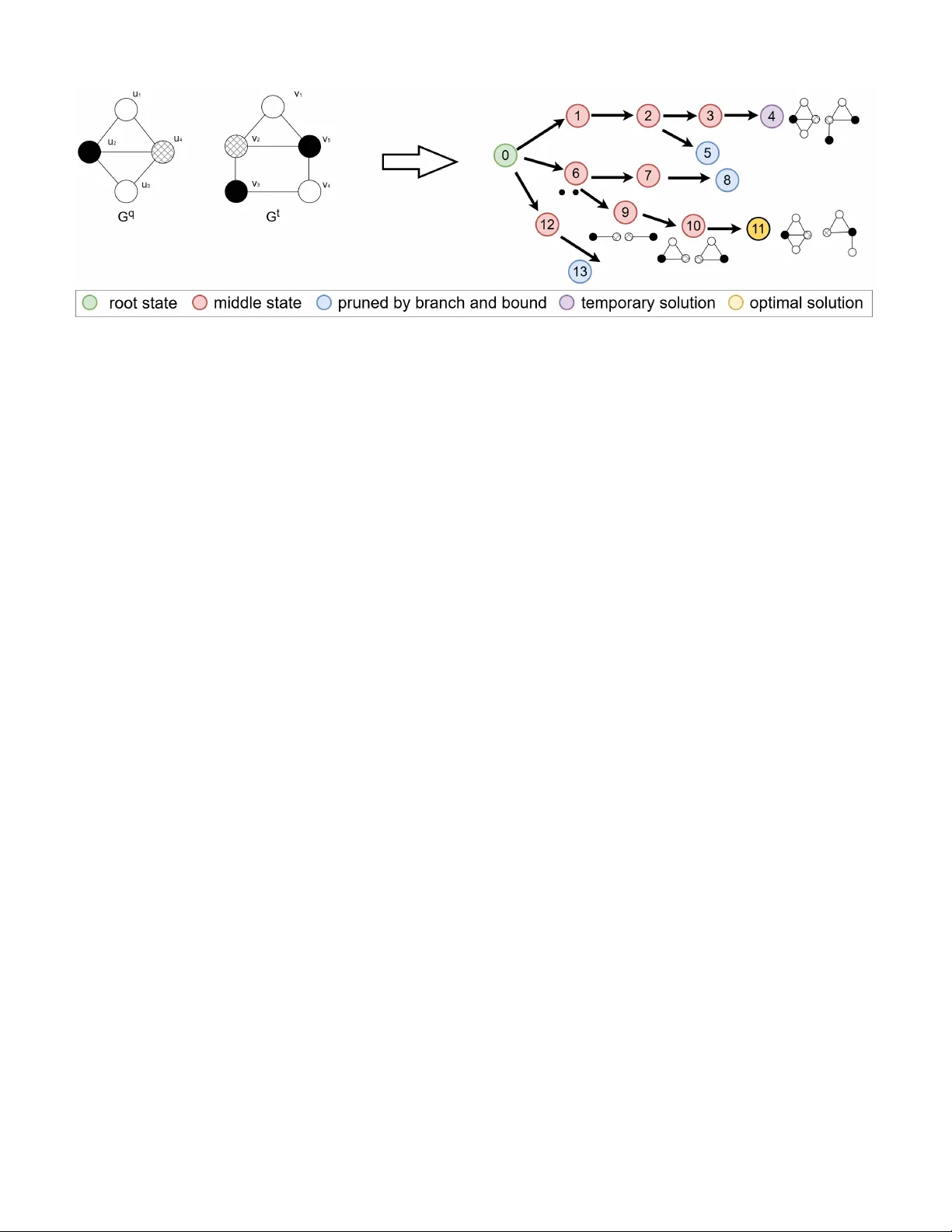
JOURNAL OF L A T E X CLASS FILES, VOL. 14, NO. 8, A UGUST 2021 1 Approximate Subgraph Matching with Neural Graph Representations and Reinforcement Learning Kaiyang Li, Shihao Ji, Senior Member , IEEE , Zhipeng Cai, F ellow , IEEE , and W ei Li Abstract —Appr oximate subgraph matching (ASM) is a task that determines the approximate presence of a giv en query graph in a large target graph. Being an NP-hard pr oblem, ASM is critical in graph analysis with a myriad of applications ranging from database systems and netw ork science to biochemistry and privacy . Existing techniques often employ heuristic search strate- gies, which cannot fully utilize the graph inf ormation, leading to sub-optimal solutions. This paper proposes a Reinfor cement Learning based Approximate Subgraph Matching (RL-ASM) algorithm that exploits graph transformers to effectively extract graph repr esentations and RL-based policies for ASM. Our model is built upon the branch-and-bound algorithm that selects one pair of nodes from the two input graphs at a time f or potential matches. Instead of using heuristics, we exploit a Graph T ransformer architecture to extract feature repr esentations that encode the full graph information. T o enhance the training of the RL policy , we use supervised signals to guide our agent in an imitation lear ning stage. Subsequently , the policy is fine-tuned with the Proximal Policy Optimization (PPO) that optimizes the accumulative long-term r ewards over episodes. Extensive experiments on both synthetic and real-w orld datasets demonstrate that our RL-ASM outperforms existing methods in terms of effectiveness and efficiency . Our source code is available at https://github .com/KaiyangLi1992/RL- ASM. Index T erms —Approximate subgraph matching, Reinf orce- ment learning, Graph T ransf ormer I . I N T R O D U C T I O N Graph analysis, a sub-field of data mining, has gained popularity in recent years as graph structured data becomes increasingly ubiquitous in a broad range of domains [1], [2]. One of the fundamental problems of graph analysis is subgraph matching, which identifies the presence of a query graph in a large target graph. Subgraph matching has a wide v ariety of applications, including database retriev al [3], knowledge graph mining [4], biomedical analysis [5], social group finding [6], and priv acy protection [7]. In most of the subgraph matching studies, the basic assump- tion is that graphs are noise-free and accurate. In order to identify an occurrence of a query graph, all nodes and edges of the query graph must occur in the target graph. In other words, the matching has to be exact. Howe ver , noise commonly exists in many real-world subgraph matching scenarios. Therefore, the Approximate Subgraph Matching (ASM) has emerged as a more practical task in graph analysis. For example, noise is prev alent in protein-protein interaction (PPI) networks [8] due Kaiyang Li and Shihao Ji are with the University of Connecticut, 352 Mansfield Road, Storrs, CT 06269, USA (e-mail: kaiyang.li@uconn.edu; shihao.ji@uconn.edu). Zhipeng Cai and W ei Li are with Georgia State University , 33 Gilmer Street SE, Atlanta, GA 30303, USA (e-mail: zcai@gsu.edu; wli28@gsu.edu). Fig. 1: An example of approximate subgraph matching, where { ( u 1 , v 1 ) , ( u 2 , v 2 ) , ( u 3 , v 4 ) , ( u 4 , v 3 ) } achie ves the best ap- proximate matching from query graph G q to target graph G t with the smallest graph edit distance of 1. to errors in data collection and varying experimental thresh- olds. By discov ering and analyzing approximate matches, biol- ogists can still validate their hypotheses based on noisy protein interaction network data. Another example is social network de-anonymization [9], which inv olves identifying anonymous individuals within a social network by correlating nodes from an auxiliary network with those from a target network, where the auxiliary network is typically a noisy subgraph. Effec- tiv e matching between these two graphs enables adversaries to launch de-anonymization attacks. Therefore, research into ASM is important to e valuate data vulnerability and de velop priv acy-preserving solutions. Formally , given a query graph G q , ASM aims to find a sub- graph in tar get graph G t that has the smallest graph edit dis- tance (GED) to G q . An example is illustrated in Fig. 1, where the mapping { ( u 1 , v 1 ) , ( u 2 , v 2 ) , ( u 3 , v 4 ) , ( u 4 , v 3 ) } achiev es the best approximate match from G q to G t with the smallest GED of 1. The existing ASM algorithms can be mainly categorized into tw o classes: (1) the methods that con v ert ASM to exact subgraph matching [10], [11], and (2) the methods that employ a branch-and-bound algorithm for combinatorial optimization [12]. The first category of methods specifies a threshold k and reduces the ASM problem to identifying all exact matches between any prototype graphs and target graph, where the prototype graphs are all graphs that can be deriv ed from the query graph with the GED smaller than k . Therefore, the exact matches of the prototype graphs are the approximate matches of the query graph. Howe ver , these methods only con- sider prototypes by adding edges to query graphs, excluding those that are derived by altering nodes’ labels. This limitation renders these methods unsuitable for scenarios where nodes’ labels are noisy . One of the reasons wh y these methods exclude prototype graphs generated by altering nodes’ labels is that doing so would significantly increase the number of prototype graphs. For example, consider a graph G q , which is a cycle JOURNAL OF L A T E X CLASS FILES, VOL. 14, NO. 8, A UGUST 2021 2 graph C 8 , where each node has 16 possible label cate gories. W ith a GED threshold k = 3 , considering only edge-induced distances, it results in 1,351 prototype graphs. Howe ver , if both edges and node labels are considered in GED, this number escalates to 347,971. On the other hand, the branch-and-bound based ASM meth- ods match one pair of nodes from query graph and tar get graph one at a time and extend intermediate results iteratively . For example, T u et al. [12] calculate the GED lower bounds of the best possible solutions within each branch of the search tree, then compare these lo wer bounds with the GED of the current best match, and prune the branches that are not possible to yield an optimal solution, i.e., the branches with lower bounds greater than the GED of the current best match. Ho wever , these methods select mapping node pairs with a greedy strate gy based on heuristics, i.e., selecting the node pair that leads to the branch with the minimized GED lo wer bound at each step by utilizing nodes’ local structural and label information. Therefore, let alone its greedy nature, the method lacks the ability of fully utilizing the graph information in the two input graphs, leading to sub-optimal solutions. T o address these limitations of the existing approaches, we introduce a Reinforcement Learning based Approximate Subgraph Matching (RL-ASM) method. RL-ASM employs a Graph Transformer [13] to extract feature representations from graphs, whose performances in graph representation learning have been extensi vely v alidated both theoretically and empirically , allo wing the use of full graph information for ASM. T o mitigate the issues induced by greedy algorithms, we train our neural network based agent with RL algorithms to optimize an accumulati ve long-term re ward over episodes. As a result, our RL-ASM achiev es the solutions that are closer to the optimal ones, outperforming the existing search algorithms by a significant margin. The contrib utions of our work are summarized as follows: • T o the best of our knowledge, RL-ASM is the first work that le verages reinforcement learning for high-quality ap- proximate subgraph matching. • Our RL-based Graph T ransformer model can fully utilize the graph information and select the node pairs by optimizing an long-term reward instead of being greedy . • Extensiv e experiments conducted on synthetic and real- world graph datasets demonstrate that RL-ASM outperforms existing methods in terms of ef fectiv eness and ef ficiency . I I . R E L ATE D W O R K T raditional ASM Methods. Being an NP-hard prob- lem [14], ASM has been tackled in various approaches. T ong et al. [15] in vestigate ASM in social networks and propose a method that samples the matched subgraph via random walk. T ian et al. [5] and Y uan et al. [16] break the query graph into small fragments and assemble the matches of these fragments to generate the entire match of the query graph. Other works [17]–[19] utilize the chi-square statistics to measure the node similarity based on the label distribution of the node’ s neighbors and apply the similarity measure to search for ASM. Sussman et al. [20] propose to calculate the permutation matrix on adjacency matrix and match query graph to target graph via the permutation matrix. Recently , Reza et al. [10] and Zhang et al. [11] identify all prototype graphs whose distances from query graph are below a specified threshold, then reduce the ASM problem to the exact subgraph matching problem by searching for exact matches between the prototype graphs and target graphs. T u et al. [12] approach the ASM problem by formulating it as a tree search problem, employing lower bounds and cutoffs to reduce the search space. Given a sufficient running time, this method can find an optimal solution, i.e., the subgraph of tar get graph that is the most similar to query graph. Unfortunately , most of the existing methods utilize hand- crafted features to search for the mapped node pairs, and can- not fully exploit the graph information for matching. What’ s more, the y all e xploit greedy algorithms that ov erlook the potential better matches in future steps, leading to sub-optimal solutions. Reinfor cement Learning for NP-hard Graph Problems. There are many prior works focusing on RL algorithms to solve NP-hard problems on graphs, including Minimum V ertex Cover [21], Network Dismantling [22], and Maximum Common Subgraph detection [23], [24]. As of exact subgraph matching, W ang et al. [25] utilize RL to determine the node mapping order on query graphs, while Bai et al. [26] utilize RL to determine the node mapping order on tar get graphs. Compared with exact subgraph matching, ASM represents an ev en more challenging task since ASM allows discrepancies between query graph G q and the matched subgragh of G t . Therefore, hard constraints that typically can be used to reduce the search space (e.g., requiring mapped nodes to ha ve the same label) are not applicable. T o address this, our RL-ASM employs a branch-and-bound algorithm to reduce the search space and lev erages a Graph T ransformer to extract graph features and select actions from a large action space. I I I . P R E L I M I N A RY A. Pr oblem Definition Let G = ( V , E ) denote a graph with a set of nodes V connected by a set of edges E . The approximate subgraph matching problem can be defined as follows. Definition 1: Appr oximate Subgraph Matching (ASM): Giv en a query graph G q = ( V q , E q ) and a target graph G t = ( V t , E t ) , ASM aims to identify a one-to-one mapping M : V q → V t such that the graph edit distance C ( M ; G q , G t ) is minimized, where C ( M ; G q , G t ) measures the discrepan- cies between query graph G q and the subgraph of G t induced by M ( V q ) . Follo wing [12], [27], we adopt the graph edit distance C ( M ; G q , G t ) over nodes and edges as C ( M ; G q , G t ) = X u ∈ V q D V ( u, M ( u )) + X e ∈ E q D E ( e, M ( e )) , (1) where the node distance is D V ( u, M ( u )) = ( 0 A ( u ) = A ( M ( u )) 1 A ( u )  = A ( M ( u )) , (2) JOURNAL OF L A T E X CLASS FILES, VOL. 14, NO. 8, A UGUST 2021 3 Fig. 2: An illustration of the search process of ASM on ( G q , G t ) . The branch-and-bound search algorithm (Algorithm 1) produces a tree structure, where each node represents a state ( s t ), the node ID reflects the order in which the state is visited, and each direct edge represents an action ( a t ), which adds a node-pair to the current node-node mapping M t . The search is essentially depth-first with pruning through the lower bound check. The policy (Line 12 of Algorithm 1) refers to a node-pair selection strategy , i.e., which state to visit next? The visiting order affects the performance of searching in the tree. For example, if state 6 can be visited before state 1, a better solution can be found in fewer iterations. This means the GED of the current best match cur rentM iniD ist will be smaller, allowing the algorithm to prune more branches in subsequent search steps. Hence, the search ef ficiency will be higher . When the search completes or a pre-defined search iteration budget is exhausted, the best solution identified by then will be returned. F or the clarity of visualization, some nodes and edges in the search tree are omitted. and the edge distance is D E ( e, M ( e )) = ( 0 e ∈ E q , M ( e ) ∈ E t 1 e ∈ E q , M ( e ) / ∈ E t . (3) Here A ( u ) denotes the label of node u . Let e be the edge between nodes u 1 and u 2 from G q , and M ( e ) refers to the edge between M ( u 1 ) and M ( u 2 ) from G t . B. The Searc h Algorithm for ASM Since the branch-and-bound search algorithm serves as the foundation of our proposed method, we first revie w a typical branch-and-bound search algorithm for ASM [12]. W e then discuss its limitations and constraints, which lead to our proposed RL-ASM. As sho wn in Algorithm 1 and Fig. 2, the branch-and-bound search algorithm, as proposed in [12], starts from an initial state with an empty mapping M 0 , and adds one pair of nodes to the mapping each time, while maintaining the best solution found so far . At each search step, denote the current search state as s t , which consists of G q , G t and the current node- node mapping M t . The algorithm attempts to select a node pair ( u, v ) , where u ∈ G q and v ∈ G t , as action a t , and add the pair to M t . As shown in Fig. 2, each action (represented by a directed edge in the search tree) updates one state to another . For e xample, action ( u 2 , v 5 ) updates state 0 to state 6, starting a branch that includes states 7-11. In [12], the authors propose a method to calculate the lower bound of C ( M ; G q , G t ) for action selection. At Line 7 of Algorithm 1, the algorithm calculates the lower bound for each branch resulting by an action from action space A t . For example, as shown in Fig. 2, when the current state is state 0, the algorithm calculates the lower bounds corresponding to the branches starting from states 1, 6, and 12. Then the algorithm compares these lo wer bounds with cur r entM iniD ist – the GED of the current best match. Any actions leading to the branches with the lo wer bounds greater than cur r entM iniDist will be eliminated from action space A t (Line 8). If all the actions in A t are eliminated, the algorithm will backtrack to the parent search state (Lines 9-11), i.e., the current branch will be cut off. When all of the nodes in G q hav e been mapped, the algo- rithm compares its C ( M t ; G q , G t ) with curr entM iniD ist . If C ( M t ; G q , G t ) is smaller , indicating a better solution than current best mapping is identified, the algorithm sets the C ( M t ; G q , G t ) as the ne w cur r entM iniDist and updates M t to M ∗ (Lines 17-20). Note that if the method can find good matches early , cur r entM iniD ist will be small, which means a lot of branches would be pruned and the search space could be reduced substantially . The above method leverages a heuristic for action selection, denoted as “polic y” at Line 12. T ypically , a greedy polic y is adopted, where the action leading to the branch with the mini- mum lower bound of GED is selected. A significant limitation of this method is that the lower bound based heuristics is not adaptiv e to the complex real-world graph structures because the method cannot fully exploit the information embedded in the graphs. More importantly , the greedy algorithm focuses on a locally optimal objecti ve for action selection at the current step without considering potential better matches in the future steps, leading to sub-optimal solutions. I V . P RO P O S E D M E T H O D In this section, we introduce our Reinforcement Learning- based Approximate Subgraph Matching (RL-ASM). W e pro- vide a high-lev el overvie w of RL-ASM in Section IV -A, including the definitions of state, action, and reward. Sec- tion IV -B describes the details of our frame work, focusing on JOURNAL OF L A T E X CLASS FILES, VOL. 14, NO. 8, A UGUST 2021 4 Algorithm 1 Branch-and-Bound for Approximate Subgraph Matching [12] Input: query graph G q and target graph G t Output: optimal node-node mapping M ∗ 1: Initalize s 0 ← ( G q , G t , M 0 = ∅ ) 2: Initalize stack ← ne w Stack( s 0 ) 3: Initalize cur r entM iniD ist ← ∞ 4: while stack  = ∅ do 5: s t ← stack .pop() 6: A t = s t .get actionspace() 7: Lbounds ← s t .get lowerbounds( A t ) 8: A t ← prune actionspace( A t , Lbounds , cur r M iniDist ) 9: if | A t | = 0 then 10: continue 11: end if 12: a t ← policy( s t , A t ) 13: A t ← A t − { a t } 14: M t ← s t .get mapping() 15: M t ← M t + a t 16: if | M t | = | V q | then 17: if C ( M t ; G q , G t ) < cur r M iniD ist then 18: cur r M iniDist ← C ( M t ; G q , G t ) 19: M ∗ ← M t 20: end if 21: continue 22: end if 23: stack .push( s t ) 24: s t +1 ← en vironment.update( s t , a t ) 25: stack .push( s t +1 ) 26: end while the design of representation learning with Graph Transformer for ASM. This is followed by Sections IV -C and IV -D, where the model training is elaborated. In Section IV -E, we discuss why structural encoding features and Graph Transformer are required for ASM. A. Overview W e formulate the ASM as a Markov Decision Process (MDP). The state s t consists of two components: (1) query graph G q and target graph G t , and (2) the current node-node mapping M t from V q to V t . Action a t : u → v is defined as adding a node pair ( u, v ) to M t , where u ∈ V q and v ∈ V t . Our policy assigns a score to each action in action space A t , and is modeled as a neural network P θ ( a t | s t ) , parameterized by θ , that computes a probability distribution over A t giv en the current state s t . For subgraph matching, the immediate re ward r t ( s t , a t ) = r node t + r edge t consists of two components: the node-matching rew ard r node t and the edge-matching reward r edge t . The node- matching reward r node t is determined by the label compatibility of the nodes added by a t : u → v , yielding +1 for identical labels and -1 otherwise. The edge-matching rew ard r edge t is defined as | E + q | − | E − q | . Here, let E q be the existing edges between node u and all the mapped nodes of G q at state s t . E + q consists of all edges e ∈ E q whose mapped edge M t ( e ) exists in E t . Con versely , E − q includes those edges e ∈ E q whose mapped edge does not exit in E t . For instance, at state 10 of Fig. 2 with M 10 = { ( u 1 , v 1 ) , ( u 2 , v 5 ) , ( u 4 , v 2 ) } and a 10 : u 3 → v 4 , E + q = { ( u 2 , u 3 ) } since ( v 4 , v 5 ) , the mapped edge, is in E t , while E − q = { ( u 3 , u 4 ) } since ( v 2 , v 4 ) , the mapped edge, is not in E t . Thus, r edge 10 = 0 . Essentially , r t ( s t , a t ) measures the change of GED after adding node pair ( u, v ) (a.k.a taking action a t ) to the current mapped subgraphs of query graph and tar get graph at state s t . If we do not impose an y constrains to the action space, the cardinality of the action space will be O ( | V q | × | V t | ) , which can be prohibitively huge. T o reduce the action space size, we generate ϕ , the mapping order of nodes in G q , before searching for subgraph matches. At each step, we take one node from G q according to the order ϕ , and map this node to one of the nodes in G t . W e generate the order ϕ with the method proposed in [28], which is designed for the e xact subgraph matching [29]. The algorithm starts by identifying the node u ∈ V q that possesses the maximum de gree, and adds it to ϕ . In the subsequent step, the algorithm prefers to add those nodes that have a larger number of edges with the nodes already present in ϕ . This is an effecti ve method to create ϕ because the node with the highest degree and the ones with more mapped neighbors typically encode substantial structural information, and thereby facilitate accurate pattern matching to initiate the search. T o enhance the efficienc y in the tree search, we further design a mechanism that caches the lo wer bounds of branches and the policy scores of actions ev aluated in pre vious steps. This allows our method to reuse cached results when back- tracking to earlier states. Because of the strong correlation between the lower bounds and the GED of current best solution cur r M inD ist [12], we delete the cached results whenev er curM inD ist is changed, and recalculate the lower bounds and the policy scores when backtracking to these states. B. The RL-ASM F ramework As sho wn in Fig. 3, our RL-ASM framew ork consists of an encoder that produces the node embeddings for V q and V t , and a decoder that transforms the embeddings into a probabilistic distribution over actions P θ ( a t | s t ) for action selection. T o design this model, we face several challenges: (i) many e xisting graph neural networks (GNNs), which primarily follow a message passing paradigm, are inherently local and their expressiv eness cannot exceed the 1-W eisfeiler-Lehman test [30]. Hence, these models lack the capability to tackle the complex approximate subgraph matching problem (see Sec- tion IV -E for justifications); (ii) as the task inv olves both query and target graphs, ef fectiv ely sharing information between the two graphs presents a significant challenge; and (iii) each state s t contains G q , G t , and the node mapping M t ; it is challenging to effecti vely encapsulate the entire state’ s information into a representation that can be utilized to predict P θ ( a t | s t ) . These challenges have guided the design of our model. 1) Node F eatur es: W e employ three distinct features for each node: (1) Label encoding : A one-hot v ector that specifies JOURNAL OF L A T E X CLASS FILES, VOL. 14, NO. 8, A UGUST 2021 5 Fig. 3: Overview of RL-ASM. RL-ASM consists of two major components: encoder and decoder . The encoder processes node label, mapping info, positional and/or structural encodings by alternating intra- and inter -components L times (with L layers) to extract po werful node representations. The decoder leverages self-attention to node embeddings of G q to generate a global state representation x s t . The action representations are then generated by the product of embeddings of node u next ∈ G q (according to ϕ ), learnable weight tensors W 3 , and embeddings of unmapped candidate nodes v 1 , v 2 , v 3 , and v 4 from G t . Subsequently , the representations of state and actions are concatenated, which is fed to a MLP and a softmax classifier to calculate the probability distrib ution over the actions P θ ( a t | s t ) . the label of each node; (2) Mapping status : A binary number indicating the node’ s mapping status - 1 if mapped, and 0 otherwise; this feature is useful to alleviate Challenge (iii); (3) Positional and structural encodings : For node’ s positional information, we utilize the Laplacian Positional Encoding (LapPE), which in v olves the eigenv ectors associated with the k smallest non-zero eigen v alues of the graph Laplacian [31]. For structural information, we apply Random W alk Structural Encoding (R WSE), deriv ed from the diagonal of the m -step random walk matrix [32]. Ramp ´ a ˇ sek et al. [13] and Kreuzer et al. [31] hav e demonstrated theoretically and empirically that using positional encoding and structural encoding in GNNs can enhance the model’ s expressi veness. Depending on the characteristics of the graph, we choose either positional or structural encoding or both as node features. This alleviates Challenge (i). Positional encoding is particularly effecti ve for image graphs [33], while structural encoding is well suited for molecular graphs [34]. Each of the three features is processed by a distinct linear layer and subsequently concatenated as the feature representations, which are fed to the encoder . 2) Encoder: The encoder consists of an intra-component module and an inter-component module as shown in Fig. 3. The intra-component module processes and aggregates mes- sages within query graph G q and target graph G t , sepa- rately . The inter-component module shares messages across the graphs based on the relationships of nodes in G q and G t . T o alle viate Challenge (i) and effecti vely utilize both local and global graph information, we employ the GraphGPS layer [13] as the intra-component. This hybrid layer combines a Message P assing Neural Network (MPNN) and a global attention mechanism, and of fers greater expressi veness than traditional MPNNs, such as GCN [35], GA T [36], and Graph- SA GE [30]. The MPNN propagates messages along the edges, whereas the global attention spreads information throughout the entire graph, as illustrated by the solid and dotted blue lines in Fig. 3. The global attention mechanism enhances this capability by passing messages across all nodes, and therefore ov ercomes the expressi veness bottleneck associated with over - smoothing and o ver-squashing [13], [37]. In each GraphGPS layer , node features are updated by integrating outputs from both the MPNN and the global attention instances. Specifi- cally , the GraphGPS layer is formulated as X ℓ + 1 in tra = GPS ℓ ( X ℓ , A ) , (4) which is implemented as X ℓ + 1 M = MPNN ℓ ( X ℓ , A ) , (5) X ℓ + 1 H = GlobalAttn ℓ ( X ℓ ) , (6) X ℓ + 1 in tra = MLP ℓ ( X ℓ + 1 M + X ℓ + 1 H ) , (7) where A ∈ R N × N is the adjacency matrix of a graph of N nodes; X ℓ ∈ R N × d denotes the d -dimensional node features for N nodes at the ℓ -th layer; MLP ℓ is a 2-layer multilayer perceptron (MLP) block; and X ℓ + 1 in tra ∈ R N × d represents the output of the intra-component at the ℓ -th layer . MPNN ℓ and GlobalAttn ℓ are modular components, which are implemented as GatedGCN [38] and Self-Attention [39], respectively . As for the inter-component module of the encoder , we employ a cross-attention mechanism that enables the model to learn ho w to share messages between G q and G t . This mechanism is established based on the node mapping rela- tionships. For state s t , the current mapping M t is { u → v | u ∈ V q t , v ∈ V t } , where V q t represents the set of nodes of G q that hav e been mapped at step t . Our method allows the nodes of G q to be mapped to nodes in G t ev en if their labels differ . Consequently , for any node u ′ ∈ G q that remains unmapped, we define its candidate set C u ′ as { v ′ ∈ V t | v ′ is unmapped in G t } . Therefore, the mapping describing the candidate relationships between nodes can be formulated as M ′ t = { u ′ → C u ′ , ∀ u ′ ∈ V q \ V q t } . Let f M t denote the union of M t and M ′ t , and f M t − 1 denote the rev erse mapping of f M t . The messages passing along M t JOURNAL OF L A T E X CLASS FILES, VOL. 14, NO. 8, A UGUST 2021 6 and M ′ t are shown as solid and dotted red lines in Fig. 3, respectiv ely . Specifically , the message passing from G q to G t is implemented as follo ws: X ℓ in ter [ u, :] = W ℓ 1 X ℓ in tra [ u, :] + X v ∈ f M t ( u ) α uv W ℓ 2 X ℓ in tra [ v , :] , (8) where X ℓ int er [ u, :] and X ℓ in tra [ u, :] ∈ R d represent inter- and intra-embeddings of node u ∈ V q at the ℓ -th layer , respectiv ely; the attention coefficients α uv are deri ved using multi-head dot-product attention [39], and W ℓ 1 and W ℓ 2 are the learnable matrices associated with the ℓ -th layer . Additionally , we implement the message passing from G t to G q following the rev erse mapping f M t − 1 . The inter-component module is crucial for information exchange across the graphs, which addresses Challenge (ii). The output from the inter-component module is then fed to an activ ation function, denoted as X ℓ + 1 = f activ ate ( X ℓ + 1 in ter ) , yielding the output of the ℓ -th encoder layer . W e construct the encoder by stacking four such layers and employ jump knowledge [40] to aggregate the outputs from these layers. 3) Decoder: The node embeddings of query graph X q ∈ R | V q |× d , produced by the encoder , capture the information from G q and from G t through the cross-graph message passing manifested by f M t and f M t − 1 . This allows X q to gather comprehensiv e information required to represent the entire state. T o alleviate Challenge (iii), we introduce an attention- based mechanism that calculates the state embedding x s t based on the embeddings of the query graph nodes as follows: x s t = Pooling ( SelfAttention ( X q )) . (9) Here, we utilize a self-attention mechanism [41] on X q , followed by aggreg ation of the resulting representations using a pooling operation. In our experiments, av erage pooling is employed for aggregation. Giv en that the policy is formulated as P θ ( a t | s t ) , it is essential to learn the representations of state s t and action a t . Consider action a t : u → v , with x u 1 and x v ∈ R d denoting the node representations learned by the encoder , we employ a bilinear tensor product defined by a learnable tensor W 3 ∈ R d × d × F to ensure sufficient interaction between the node embeddings in volv ed by action. Here, F is a hyperparam- eter that enhances the model’ s capacity by adding dimensions to learn complex relationships. Then action a t : u → v can be expressed as x T u W 3 x v , which is concatenated with the state embedding x s t . The combined v ector is then fed into a multi-layer perceptron (MLP), followed by a softmax layer to generate P θ ( a t | s t ) = SoftMax ( MLP ( CONCA T ( x s t , x T u W 3 x v ))) . (10) C. P olicy T raining The goal of policy training is to maximize the accumulativ e long-term reward: R t = P T i = t γ i − t r i , where T is the total number of time steps of an episode, γ is the discount factor , 1 Here, u is the next node selected from G q according to the order ϕ . and r i is the immediate reward incurred by action a i at the i -th step. T o enhance training efficienc y , we disable the backtracking mechanism during the policy training. That is, once our algorithm reaches to a leaf node in the search tree, the episode ends. W e employ the Proximal Policy Optimization (PPO) [42], one of the most effecti ve policy gradient methods, to train our model. PPO mitigates excessi vely lar ge policy changes by clipping policy probability ratios, which helps maintain stability in the learning process. The core term of the PPO loss function is defined as L clip ( θ ) = − ˆ E t h min  ρ ( θ ) ˆ R t , clip( ρ ( θ ) , 1 − ε, 1 + ε ) ˆ R t  i , (11) where ˆ E t [ · ] indicates the empirical average ov er a batch of samples, ρ ( θ ) = P θ ( a t | s t ) P θ old ( a t | s t ) is the ratio of the action probabilities under current and old policy , and ˆ R t denotes the accumulated re ward, normalized across the batch. The operation clip( ρ ( θ ) , 1 − ε, 1 + ε ) ˆ R t modifies the objectiv e by clipping the probability ratio, thereby moderating the influence of extreme policy changes during the training. T o ensure sufficient exploration and pre vent premature con vergence to a local optimal policy , we also incorporate an entropy bonus term to the loss function: L entrop ( θ ) = − ˆ E t [ H ( P θ ( ·| s t ))] , (12) where H ( · ) is the entropy of the probability distribution ov er action space A t giv en state s t . The overall objective function of PPO is L P P O ( θ ) = L clip ( θ ) + cL entrop ( θ ) , (13) where c is a hyperparameter that balances the contributions from the two loss terms. D. Pr e-training For graph pairs of large graphs, the action space can be huge. T o expedite the learning process and enhance sample efficienc y , we pre-train our model with imitation learning be- fore the PPO fine-tuning. This pre-training in volves sampling subgraphs from the target graph and recording the correspon- dence between nodes of the sampled and target graphs to define expert actions. Noise is added to these sampled graphs to generate query graphs. In this pre-training stage, the model’ s predictions are compared to the expert’ s choices, with training conducted using a supervised cross-entropy loss: L I mit ( θ ) = − X a ∈ A t y a log( ˆ y a ( θ )) , (14) where y a indicates whether the action a aligns with the expert’ s choice (1 for yes, 0 for no), and ˆ y a represents the predicted probability corresponding to action a . Note that during imitation learning, we enable Dropout and Batch Normalization in the model, whereas in the PPO fine-tuning, we disable these components to improve the training stability . JOURNAL OF L A T E X CLASS FILES, VOL. 14, NO. 8, A UGUST 2021 7 Fig. 4: Example graphs that are indistinguishable by MPNN. E. Why ar e LapPE and Graph T ransformer Needed for ASM? The encoder of RL-ASM consists of an intra-component module and an inter-component module. In the inter - component, messages are passed along f M and f M − 1 , which denote the edges between the nodes in G q and G t . This implies that the inter-component can be considered as an MPNN. Therefore, if we employ traditional MPNN architectures (e.g., GCN, GA T , or GatedGCN) as the intra-component of our encoder , the entire architecture will be an MPNN. It has been prov en that the expressi veness of MPNNs cannot exceed the 1- W eisfeiler-Lehman test [30]. That is, they cannot differentiate non-isomorphic graphs by using only 1-hop neighborhood aggregation. In Fig. 4, when only the labels of nodes (which correspond to node colors in the figure) are used as input features, the MPNN fails to distinguish between G t 1 and G t 2 because the nodes with the identical ID in G t 1 and G t 2 hav e the same 1-hop neighborhood structure. Consequently , when attempting to match query graph G q with G t 1 and G t 2 , an MPNN-based model will yield identical matching results. Howe ver , the optimal matching solutions for these cases are different; one is { (1,1), (2,2), (3,3), (4,4) } and another one is { (1,5), (2,2), (3,3), (4,4) } . This example illustrates the expressi veness limitation of MPNNs when addressing the ASM problem. Kreuzer et al. [31] demonstrate that with the full set of Laplacian eigenv ectors, a Graph T ransformer model can be a universal function approximator on graphs and can pro vide an approximate solution to the graph isomorphism problem. This suggests that by inte grating LapPE and GraphGPS (a type of Graph T ransformer) into the model, our RL-ASM has the capability beyond the traditional MPNN models in solving the ASM problem. V . E X P E R I M E N T S In this section, we compare our RL-ASM with state-of-the- art approaches for ASM, and demonstrate its effecti veness and efficienc y . All our experiments were conducted using a server equipped with Intel Xeon Gold 6242 CPUs and NVIDIA T esla V100 GPUs. For reproducible research, we provide our source code at https://github.com/KaiyangLi1992/RL- ASM. A. Datasets Our experiments utilize one synthetic dataset and three real-world datasets from div erse domains: biology , computer Dataset SYNTHETIC AIDS MSRC 21 Email T arget size (nodes) 100 17.03 77.48 1005 T arget size (edges) 196 17.58 198.18 25571 Query size (nodes) 15.75 8.09 24.12 13.19 Query size (edges) 18.13 8.24 57.29 60.04 Num. of Node Labels 13 40 27 47 Sampling range of | V q | [10, 20] [6, 10] [16, 32] [8, 16] T ABLE I: Statistics of query graphs and target graphs. vision, and social networks. These datasets are described as follows: • SYNTHETIC [43]: This dataset comprises 300 synthetic graphs generated by a statistical model. Each graph consists of 100 nodes and 196 edges, and each node is endowed with a normally distributed scalar label. • AIDS [43]: This dataset contains 2,000 graphs, each rep- resenting a molecular compound. Nodes in these graphs correspond to atoms, while edges represent the chemical bonds between them. • MSRC 21 [43]: As a semantic image processing bench- mark, this dataset includes 563 graphs, each representing the graphical model of an image. Nodes in the graph represent objects in an image, and edges illustrate the relationships among the objects. • EMAIL [44]: Originating from an email communication network at a European research institution, this dataset uses nodes to represent employees, and edges to represent the email interactions between employees. The node label indicates the department to which each employee belongs. For datasets SYNTHETIC , AIDS , and MSRC 21 , which contain multiple graphs, we randomly select graphs from these collections to serv e as the target graphs. For the EMAIL dataset, which contains a single graph, we use this graph consistently as the target graph. W e employ the Breadth-First Search (BFS) on these target graphs to sample nodes, ceasing the sampling when the node count reaches the parameters specified in T able I. From these sampled nodes, induced sub- graphs are generated to form the seed query graphs. W e then introduce noise to these seed query graphs by adding edges and altering node labels, thereby producing query graphs with noise le vels of 0%, 5%, and 10%. Specifically , we calculate the total number of nodes and edges in each query graph, multiply this total number by the noise le vel to determine the noise intensity , N noise . W e then randomly select an integer N node noise between 0 and N noise , change the labels of N node noise nodes, and add N noise − N node noise edges to the original query graph, thereby generating a noisy query graph. Each pair of a query graph and its corresponding original target graph constitutes a graph pair for ASM. After eliminating duplicate graph pairs, we partition the dataset into training, v alidation, and test sets following an 8:1:1 ratio. The statistics of the query and target graphs are reported in T able I. T o closely simulate real-world conditions, we operate under the assumption that the noise lev el in query graphs remains unknown. T o ensure our model adapts broadly , our training and validation sets for each dataset encompass query graphs from all three noise levels: 0%, 5%, and 10%. Howe ver , for the purpose of e v aluation, we specifically test our model’ s performances on these noise levels to report its performances JOURNAL OF L A T E X CLASS FILES, VOL. 14, NO. 8, A UGUST 2021 8 T raining Stage Hyperparameter AIDS SYNTHETIC MSRC 21 EMAIL Hidden Dimension 32 32 32 32 # Encoder Layers 4 4 4 4 Interaction Dimension F 32 32 32 32 Positional and Structural Encodings R WSE R WSE LapPE R WSE Imitation Learning Batch Size 1024 1024 1024 1024 Learning Rate 0.001 0.0005 0.001 0.001 #Epochs 1000 1000 1000 1000 W eight Decay 0.01 0.01 0.01 0.01 PPO Fine-tuning Learning Rate 0.005 0.001 0.0005 0.0005 Entropy Coefficient 0.01 0.01 0.01 0.01 Batch Size 2048 512 1024 64 # Epochs 10 10 10 10 γ 0.99 0.99 0.99 0.99 Clipping Range 0.2 0.2 0.2 0.2 T ABLE II: The hyperparameters of RL-ASM used for dif ferent benchmark datasets. under different conditions. B. Baselines W e compare our method with a neural-network based method NeuroMatch [45] and two heuristic methods ISM [12] and APM [10]. As shown in Fig. 2, a good initial matching solution is crucial for the search performance of branch-and- bound methods. Therefore, we present the first-round matching results (i.e., the results without backtracking) for both ISM and our method in this section. Additionally , we emphasize the role of imitation learning as an important pre-training stage of our method, showcasing the performances of our model when trained exclusiv ely through imitation learning. W e benchmark against the following methods: • NeuroMatch [45] decomposes query and target graphs into small subgraphs and embeds them using graph neu- ral networks. It first predicts the probability of nodes in query graphs matching to nodes in target graphs with the embeddings of the decomposed subgraphs. It then utilizes the Hungarian algorithm [46] to map the nodes between the two graphs such that the sum of the probabilities of the matched node pairs is maximized with the constraint that each node in query graph is assigned to a different node in target graph. • APM [10] reduces ASM to exact subgraph matching. It focuses on identifying exact matches between prototype graphs (i.e., those deriv ed from the query graph with GED below a specific threshold) and target graphs. T o av oid an excessi vely large search space, the method only considers prototypes that are derived by adding edges to query graphs, excluding those that are deri ved by altering nodes’ labels. • ISM [12] formulates ASM as a tree search problem. It calculates the lower bound of the GED between query graph and the corresponding subgraph in target graph within each search branch from the current step. The branches, whose lower bounds surpass the GED of the best match found so far , are pruned. The method employs a greedy strategy to select the node pair that leads to the branch with the minimal lower bound at each search step. • RL-ASM-IL showcases the first-round mapping results of our RL-ASM, which is trained exclusi vely through imitation learning. This illustrates the impact of imitation learning to our model. • RL-ASM-FR and ISM-FR illustrate the first-round match- ing results of RL-ASM and ISM without backtracking. For the experiments of ISM and RL-ASM, we limit the search tree exploration to 600 seconds. If the programs fail to trav erse the entire tree within this time limit, we terminate the ex ecution and treat the best matching result found so far as the final outcome. The hyperparameters of RL-ASM used for different bench- mark datasets are provided in T able II. W e select the best model according to the metric on the validation set and report the metric on the test set. Specifically , the learning rates for imitation learning and PPO fine-tuning are selected from { 5e- 5, 1e-4, 5e-4, 1e-3, 5e-3, 1e-2 } . W e search for the hidden dimension of nodes from { 16, 32, 64 } for RL-ASM. C. Results 1) Effectiveness of Appr oximate Subgraph Matching: The graph edit distance (GED), as reported in T able III, quantifies the discrepancies between the query graph and its correspond- ing subgraph in the tar get graph, with smaller v alues indicating better matches. The results of RL-ASM-IL indicate that e ven when trained solely via imitation learning, our model’ s initial matching results significantly outperform the heuristic meth- ods: APM and ISM. This demonstrates our model’ s ability to effecti vely learn graph information via Graph T ransformer for ASM. Compared with NeuroMatch and RL-ASM-IL, RL- ASM-FR shows superior performance on the SYNTHETIC , MSRC 21 , and EMAIL datasets. This impro vement attrib utes to the RL training phase, which maximizes an accumula- tiv e long-term reward. The enhancements observed from RL training on the MSRC 21 and EMAIL datasets are more pronounced compared to the AIDS dataset. This is because the graphs in MSRC 21 and EMAIL are much larger and more challenging, requiring the model to engage in optimizing long-term rewards and explore a broader solution space, the areas where RL excels. RL-ASM deliv ers the best results by effecti vely searching the trees with backtracking to find better subgraph matches be yond the results of RL-ASM-FR. In the following subsection, we will demonstrate that our model, guided by a neural network, can potentially identify optimal solutions within a constrained time limit. When no noise is added to query graphs (e.g., noise ratio 0% ), APM can find the optimal solution because it reduces the JOURNAL OF L A T E X CLASS FILES, VOL. 14, NO. 8, A UGUST 2021 9 T ABLE III: Graph Edit Distance (GED) between query graph and its matched subgraph identified from target graph. Note that the “GroundTruth” number denotes the GED between the “noisy” query graph and its corresponding seed query graph sampled from target graph. Dataset SYNTHETIC AIDS MSRC 21 EMAIL Noise Ratio 0% 5% 10% 0% 5% 10% 0% 5% 10% 0% 5% 10% GroundT ruth 0.00 1.70 3.39 0.00 1.00 1.67 0.00 3.99 8.03 0.00 3.66 7.32 NeuroMatch [45] 1.52 4.42 7.96 0.80 3.12 7.49 3.56 11.46 22.43 3.71 17.41 26.51 APM [10] 0.00 2.45 4.57 0.00 1.24 2.43 0.00 7.46 13.43 0.00 8.11 15.61 ISM-FR 8.14 9.13 11.03 0.79 1.91 2.92 18.50 21.66 26.87 4.97 11.25 13.32 ISM [12] 7.00 8.35 10.60 0.01 1.04 2.00 17.07 20.69 26.26 4.67 10.74 12.90 RL-ASM-IL 0.00 1.65 3.40 0.06 1.16 1.85 0.01 4.29 8.93 0.00 3.65 7.00 RL-ASM-FR 0.00 1.59 3.31 0.06 1.17 1.84 0.00 4.19 8.93 0.00 3.56 6.63 RL-ASM (ours) 0.00 1.54 3.18 0.00 1.04 1.77 0.00 4.07 8.77 0.00 3.13 6.09 (a) AIDS (b) SYNTHETIC (c) MSRC 21 (d) EMAIL Fig. 5: The probabilities that ISM and our method find the optimal solutions within 600s. ASM to an exact subgraph matching problem. For each graph pair , it attempts to match G q and G t using an exact subgraph mapping method, which can consistently identify the optimal solution when query graph G q contains no noise. Howe ver , the performance of APM declines when handling noisy instances of G q as it does not allow mappings between node pairs with differing labels. For ISM, which selects actions based on heuristics, it struggles to find effecti ve solutions in the initial round, as manifested by the results of ISM-FR in T able III. This limi- tation hinders its ability to prune numerous branches during tree searches. Moreover , the greedy search utilizes heuristics to make decision at each step. Consequently , both its initial and final mappings are prone to sub-optimal. In addition, NeuroMatch is designed for exact subgraph matching; when noise is added to the query graph, it struggles to map nodes accurately based on the learned representations. 2) Efficiency of Appr oximate Subgraph Matching: Both ISM and RL-ASM utilize a branch-and-bound frame work to effecti vely search the entire tree to find the optimal solution. Fig. 5 illustrates the efficiencies of ISM and our method by reporting the probability of each method finding the optimal solution within 600 seconds. The results reveal that our method, guided by a neural network for action selection, is significantly more ef ficient than ISM. While both methods perform similarly with smaller graphs, such as the instances in the AIDS dataset, the efficiency gap is more pronounced with larger graphs. For example, on the SYNTHETIC dataset, our method significantly outperforms ISM, achieving a probability of identifying the optimal solution that is about 5x higher than T ABLE IV: Ablation study of design choices on node-sorting and GraphGPS. Dataset SYNTHETIC Noise-Ratio 0% 5% 10% RL-ASM w/o node-sorting 0 1.63 3.38 RL-ASM w/o GraphGPS 0 1.67 3.47 RL-ASM 0 1.54 3.18 that of ISM. 3) Ablation Study: In Section IV, we introduce a method based on [28] to sort the nodes in G q for mapping order ϕ , and we also utilize GraphGPS [13], a type of graph transformer, as the intra-component in our encoder . This section assesses the impact of these design choices by replacing the sorted node order with a random node order or substituting GraphGPS with GatedGCN, which inv olves removing the global attention from the intra-component of our encoder . T able IV presents the results of these ablation studies. It is observed that both node sorting ϕ and GraphGPS enhance the performance of our RL-ASM. The node sorting prioritizes nodes with higher degrees and more matched neighbors, lev eraging the structural information to facilitate accurate pattern matching. Moreov er , GraphGPS, integrating an MPNN with global attention, sig- nificantly increases the e xpressiveness of our model. 4) Generalization: In the experiments above, we utilize the BFS to sample subgraphs and produce induced subgraphs (a.k.a query graphs) from the sampled nodes. In this section, we adopt a Random W alk (R W) approach for query graph sampling. Specifically , we start at a randomly selected node and move to an adjacent node with random walk, repeating JOURNAL OF L A T E X CLASS FILES, VOL. 14, NO. 8, A UGUST 2021 10 T ABLE V: Effecti veness on the random walk sampled dataset. Dataset SYNTHETIC Noise-Ratio 0% 5% 10% ASP 0 2.03 4.04 ISM 5.58 7.69 8.51 RL-ASM 0 1.47 3.42 Fig. 6: Efficiency on the random w alk sampled dataset. this process for a pre-determined number of steps. During this process, we record all visited nodes and edges to construct the query graphs. Note that the R W sampled subgraphs may not necessarily be the induced subgraphs. Subsequently , we introduce noise to these sampled graphs to create noisy query graphs. This methodology is applied to the SYNTHETIC dataset to create training, v alidation, and test sets, which are used to assess the performance of ASM in volving non-induced subgraphs. The GED between G q and the matched subgraphs, along with the probability of identifying the optimal solutions within 600 seconds, are reported in T able V and Fig. 6, respec- tiv ely . The results indicate that our model still outperforms the baseline methods in terms of ef fectiv eness and efficienc y , ev en when the query graphs are not induced ones, demonstrating the generalization of RL-ASM. V I . C O N C L U S I O N As an NP-hard problem, approximate subgraph matching (ASM) is a fundamental research task in the database and graph mining communities. One significant strand of ASM methods follows the branch-and-bound search framew ork, where search performance is heavily influenced by the selec- tion of actions (i.e., the mapped node pairs) in the search tree. W e observ e that e xisting methods, which utilize heuristics to select actions, lack the capability to fully exploit the struc- tural and label information of graphs, and make sub-optimal decisions for ASM. In this paper, we introduce RL-ASM, a reinforcement learning based method for ASM that lev erages Graph Transformer to extract the full graph information and optimizes an accumulativ e long-term rew ards o ver episodes for ASM. Extensive experiments demonstrate the effecti veness and efficiency of our approach on four benchmark datasets. ASM is a relati vely less inv estigated research area. W e open source our code to facilitate the research in this area. R E F E R E N C E S [1] C. C. Aggarw al, H. W ang et al. , Managing and mining gr aph data . Springer , 2010, vol. 40. [2] D. Chakrabarti and C. Faloutsos, Graph mining: laws, tools, and case studies . Springer Nature, 2022. [3] L. Zou, J. Mo, L. Chen, M. T . ¨ Ozsu, and D. Zhao, “gstore: answering sparql queries via subgraph matching, ” Pr oc. VLDB Endow . , vol. 4, no. 8, p. 482–493, may 2011. [Online]. A v ailable: https://doi.org/10.14778/2002974.2002976 [4] S. Hu, L. Zou, J. X. Y u, H. W ang, and D. Zhao, “ Answering natural language questions by subgraph matching over knowledge graphs, ” IEEE T ransactions on Knowledge and Data Engineering , vol. 30, no. 5, pp. 824–837, 2018. [5] Y . Tian, R. C. Mceachin, C. Santos, D. J. States, and J. M. Patel, “Saga: a subgraph matching tool for biological graphs, ” Bioinformatics , vol. 23, no. 2, pp. 232–239, 2007. [6] W . Fan, “Graph pattern matching revised for social network analysis, ” in Pr oceedings of the 15th International Conference on Database Theory , ser . ICDT ’12. New Y ork, NY , USA: Association for Computing Machinery , 2012, p. 8–21. [Online]. A vailable: https://doi.org/10.1145/2274576.2274578 [7] G. Lu, K. Li, X. W ang, Z. Liu, Z. Cai, and W . Li, “Neural-based inexact graph de-anonymization, ” High-Confidence Computing , vol. 4, no. 1, p. 100186, 2024. [8] M. Zaslavskiy , F . Bach, and J.-P . V ert, “Global alignment of protein– protein interaction netw orks by graph matching methods, ” Bioinformat- ics , vol. 25, no. 12, pp. i259–1267, 2009. [9] S. Ji, P . Mittal, and R. Beyah, “Graph data anonymization, de- anonymization attacks, and de-anonymizability quantification: A sur- vey , ” IEEE Communications Surve ys & T utorials , v ol. 19, no. 2, pp. 1305–1326, 2016. [10] T . Reza, M. Ripeanu, G. Sanders, and R. Pearce, “ Approximate pattern matching in massiv e graphs with precision and recall guarantees, ” in Pr oceedings of the 2020 ACM SIGMOD International Confer ence on Management of Data , 2020, pp. 1115–1131. [11] S. Zhang, J. Y ang, and W . Jin, “Sapper: Subgraph inde xing and approx- imate matching in lar ge graphs, ” Pr oceedings of the VLDB Endowment , vol. 3, no. 1-2, pp. 1185–1194, 2010. [12] T . K. T u, J. D. Moorman, D. Y ang, Q. Chen, and A. L. Bertozzi, “Inexact attributed subgraph matching, ” in 2020 IEEE international conference on big data (big data) . IEEE, 2020, pp. 2575–2582. [13] L. Ramp ´ a ˇ sek, M. Galkin, V . P . Dwiv edi, A. T . Luu, G. W olf, and D. Beaini, “Recipe for a general, powerful, scalable graph transformer, ” Advances in Neural Information Pr ocessing Systems , vol. 35, pp. 14 501–14 515, 2022. [14] M. R. Garey and D. S. Johnson, Computers and Intractability: A Guide to the Theory of NP-Completeness . New Y ork: W . H. Freeman and Company , 1979. [15] H. T ong, C. Faloutsos, B. Gallagher , and T . Eliassi-Rad, “Fast best-effort pattern matching in large attributed graphs, ” in Pr oceedings of the 13th ACM SIGKDD international confer ence on Knowledge discovery and data mining , 2007, pp. 737–746. [16] Y . Y uan, G. W ang, J. Y . Xu, and L. Chen, “Efficient distributed subgraph similarity matching, ” The VLDB Journal , vol. 24, no. 3, pp. 369–394, 2015. [17] S. Dutta, P . Nayek, and A. Bhattacharya, “Neighbor-aw are search for approximate labeled graph matching using the chi-square statistics, ” in Pr oceedings of the 26th International Conference on W orld W ide W eb , 2017, pp. 1281–1290. [18] S. Agarwal, S. Dutta, and A. Bhattacharya, “V enom: Approximate sub- graph matching with enhanced neighbourhood structural information, ” in Pr oceedings of the 7th Joint International Confer ence on Data Science & Management of Data (11th ACM IKDD CODS and 29th COMAD) , 2024, pp. 18–26. [19] ——, “Chisel: Graph similarity search using chi-squared statistics in large probabilistic graphs, ” Pr oceedings of the VLDB Endowment , vol. 13, no. 10, pp. 1654–1668, 2020. [20] D. L. Sussman, Y . Park, C. E. Priebe, and V . L yzinski, “Matched filters for noisy induced subgraph detection, ” IEEE tr ansactions on pattern analysis and machine intelligence , vol. 42, no. 11, pp. 2887–2900, 2019. [21] E. Khalil, H. Dai, Y . Zhang, B. Dilkina, and L. Song, “Learning combinatorial optimization algorithms over graphs, ” Advances in neural information pr ocessing systems , vol. 30, 2017. [22] C. Fan, L. Zeng, Y . Sun, and Y .-Y . Liu, “Finding key players in com- plex networks through deep reinforcement learning, ” Natur e machine intelligence , vol. 2, no. 6, pp. 317–324, 2020. [23] Y . Liu, C.-M. Li, H. Jiang, and K. He, “ A learning based branch and bound for maximum common subgraph related problems, ” in Pr oceedings of the AAAI Conference on Artificial Intelligence , vol. 34, no. 03, 2020, pp. 2392–2399. JOURNAL OF L A T E X CLASS FILES, VOL. 14, NO. 8, A UGUST 2021 11 [24] Y . Bai, D. Xu, Y . Sun, and W . W ang, “Glsearch: Maximum common subgraph detection via learning to search, ” in International Confer ence on Machine Learning . PMLR, 2021, pp. 588–598. [25] H. W ang, Y . Zhang, L. Qin, W . W ang, W . Zhang, and X. Lin, “Re- inforcement learning based query vertex ordering model for subgraph matching, ” in 2022 IEEE 38th International Conference on Data Engi- neering (ICDE) . IEEE, 2022, pp. 245–258. [26] Y . Bai, D. Xu, Y . Sun, and W . W ang, “Detecting small query graphs in a large graph via neural subgraph search, ” arXiv pr eprint arXiv:2207.10305 , 2022. [27] H. He and A. K. Singh, “Closure-tree: An index structure for graph queries, ” in 22nd International Conference on Data Engineering (ICDE’06) . IEEE, 2006, pp. 38–38. [28] V . Bonnici, R. Giugno, A. Pulvirenti, D. Shasha, and A. Ferro, “ A subgraph isomorphism algorithm and its application to biochemical data, ” BMC bioinformatics , vol. 14, pp. 1–13, 2013. [29] S. Sun and Q. Luo, “In-memory subgraph matching: An in-depth study , ” in Proceedings of the 2020 A CM SIGMOD International Confer ence on Management of Data , 2020, pp. 1083–1098. [30] K. Xu, W . Hu, J. Leskovec, and S. Jegelka, “How po werful are graph neural networks?” in International Conference on Learning Repr esentations , 2019. [Online]. A vailable: https://openreview .net/ forum?id=ryGs6iA5Km [31] D. Kreuzer, D. Beaini, W . Hamilton, V . L ´ etourneau, and P . T ossou, “Rethinking graph transformers with spectral attention, ” in Advances in Neur al Information Pr ocessing Systems , M. Ranzato, A. Beygelzimer , Y . Dauphin, P . Liang, and J. W . V aughan, Eds., vol. 34. Curran Associates, Inc., 2021, pp. 21 618– 21 629. [Online]. A vailable: https://proceedings.neurips.cc/paper files/ paper/2021/file/b4fd1d2cb085390fbbadae65e07876a7- Paper .pdf [32] V . P . Dwiv edi, A. T . Luu, T . Laurent, Y . Bengio, and X. Bresson, “Graph neural networks with learnable structural and positional representations, ” arXiv preprint arXiv:2110.07875 , 2021. [33] K. Han, Y . W ang, J. Guo, Y . T ang, and E. Wu, “V ision gnn: An image is worth graph of nodes, ” Advances in neural information processing systems , vol. 35, pp. 8291–8303, 2022. [34] R. Sun, H. Dai, and A. W . Y u, “Does gnn pretraining help molecular representation?” Advances in Neural Information Pr ocessing Systems , vol. 35, pp. 12 096–12 109, 2022. [35] T . N. Kipf and M. W elling, “Semi-supervised classification with graph con volutional networks, ” arXiv preprint , 2016. [36] P . V eli ˇ ckovi ´ c, G. Cucurull, A. Casanova, A. Romero, P . Lio, and Y . Ben- gio, “Graph attention netw orks, ” arXiv pr eprint arXiv:1710.10903 , 2017. [37] S. Akansha, “Over-squashing in graph neural networks: A comprehen- siv e survey , ” arXiv pr eprint arXiv:2308.15568 , 2023. [38] Y . Li, R. Zemel, M. Brockschmidt, and D. T arlow , “Gated graph sequence neural networks, ” in Proceedings of ICLR’16 , 2016. [39] A. V aswani, N. Shazeer , N. Parmar , J. Uszkoreit, L. Jones, A. N. Gomez, Ł. Kaiser, and I. Polosukhin, “ Attention is all you need, ” Advances in neural information pr ocessing systems , vol. 30, 2017. [40] K. Xu, C. Li, Y . T ian, T . Sonobe, K.-i. Kawarabayashi, and S. Jegelka, “Representation learning on graphs with jumping kno wledge netw orks, ” in International conference on machine learning . PMLR, 2018, pp. 5453–5462. [41] P . Shaw , J. Uszkoreit, and A. V aswani, “Self-attention with relative position representations, ” in Pr oceedings of the 2018 Conference of the North American Chapter of the Association for Computational Linguistics: Human Language T echnologies, V olume 2 (Short P apers) , 2018, pp. 464–468. [42] J. Schulman, F . W olski, P . Dhariwal, A. Radford, and O. Klimov , “Prox- imal policy optimization algorithms, ” arXiv pr eprint arXiv:1707.06347 , 2017. [43] C. Morris, N. M. Krie ge, F . Bause, K. Kersting, P . Mutzel, and M. Neumann, “Tudataset: A collection of benchmark datasets for learning with graphs, ” in ICML 2020 W orkshop on Graph Repr esentation Learning and Beyond (GRL+ 2020) , 2020. [Online]. A vailable: www .graphlearning.io [44] J. Leskov ec, J. Kleinberg, and C. Faloutsos, “Graph ev olution: Den- sification and shrinking diameters, ” A CM transactions on Knowledge Discovery fr om Data (TKDD) , vol. 1, no. 1, pp. 2–es, 2007. [45] Z. Lou, J. Y ou, C. W en, A. Canedo, J. Leskovec et al. , “Neural subgraph matching, ” arXiv preprint , 2020. [46] H. W . Kuhn, “The Hungarian method for the assignment problem, ” Naval resear ch logistics quarterly , vol. 2, no. 1-2, pp. 83–97, 1955.