Towards sample-optimal learning of bosonic Gaussian quantum states

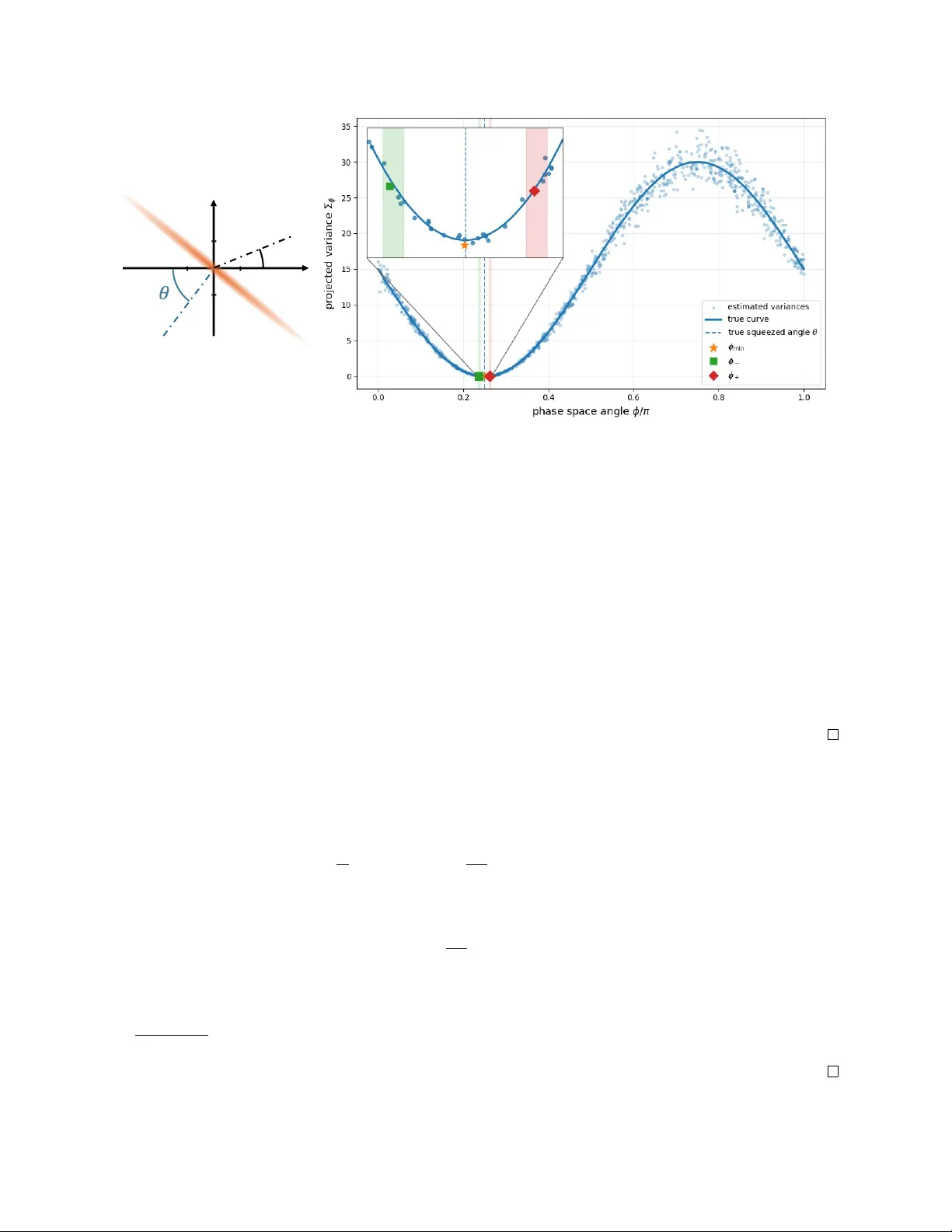
T o wards sample-optima l learning o f boso nic Gau ssi an qu antum st ates Senrui Chen ∗ 1 , Fran cesco Anna Mele † 2 , Marco F anizz a 3 , Alfred Li 1 , Zachary Mann 1 , Hsin- Y uan Huang 1 , Y anbei Chen 1 , and J ohn Preskill ‡ 1 1 Institute for Quantum Inf ormation and Matter , Ca ltech, P asadena, CA 91125, US A 2 Scuola Norma le Superiore, Piazza dei Cava lieri 7, 56126 Pisa, It aly 3 Inria, T élécom P aris – L TCI, Institut P olytechnique de P aris, France March 20, 2026 Abstract Continu ous-varia ble sy stems en ab le key quantum technol ogies in computation, co mmunicati on, and sensing. Boso nic Gaussian states emerge naturally in vari ous su ch applicati ons, including gravitatio n al-w av e and dark-matter detectio n. A f undamental questio n is how to characterize an unkno wn bosoni c Gaussian st ate from a s few samples as possib le. Despite decades-l ong exploratio n, the ultimate efficien cy limit remains unclear . In this work, we study the necessary and sufficient number o f copies t o learn an n -m ode Gaussian state, with energy less than E , to ε trace distance closen ess with high probabilit y . W e prov e a lo wer bound o f Ω( n 3 /ε 2 ) for Gaussian measurements, matching the best kno wn upper bound up to doubly-l og energy dependence, and Ω( n 2 /ε 2 ) for arbitrary measurements. W e f urther sho w an upper bound of e O ( n 2 /ε 2 ) giv en that the Gaussian state is promised to be either pure or passiv e. Interestingly , while Gaussian measurements suffice for nearly optimal learning of pure Gaussian st ates, non-Ga ussian measurements are prov ably required for optimal learning of passiv e Gaussian st ates. Finally , focusing on learning single-m ode Gaussian states via non-entangling Gaussian mea surements, we provide a nearly tight bound of e Θ( E /ε 2 ) for any non-adapti ve schemes, sho wing adaptivit y is indispensab le for nearly energy-independent scaling. As a key technical tool o f independent interest, we est ab lish stringent bounds on the trace distance bet ween Gaussian st ates in terms o f the total variation dist ance bet ween their Wigner f uncti ons. In particular , this yields a nearly tight sample complexit y of e Θ( n 2 /ε 2 ) for learning the Wign er distributi on of any Gaussian state to ε total variation dist ance, achieva ble with Gaussian measurements. Our results greatly advance quantum learning theory in the bosonic regimes and hav e practica l impact in quantum sensing and benchmarking applicati ons. ∗ csenrui@gmail.com † francesco.mele@sns.it ‡ preskill@caltech.edu 1 Contents 1 Introd uctio n 2 2 Preliminaries 5 3 R esults 5 3.1 W arm-up: L earning Gaussian Wign er distributi ons . . . . . . . . . . . . . . . . . . . . 5 3.2 Low er bounds on Gaussian st ate learning . . . . . . . . . . . . . . . . . . . . . . . . . 8 3.3 Upper bounds on Gaussian state learning . . . . . . . . . . . . . . . . . . . . . . . . . 9 3.4 On Energy Dependence . . . . . . . . . . . . . . . . . . . . . . . . . . . . . . . . . . . 11 4 Discussio n 13 4.1 Pri or works and context of our results . . . . . . . . . . . . . . . . . . . . . . . . . . . 13 4.2 Open probl ems . . . . . . . . . . . . . . . . . . . . . . . . . . . . . . . . . . . . . . . 15 4.3 P otential practica l appli cations . . . . . . . . . . . . . . . . . . . . . . . . . . . . . . . 16 Ackno wledgments 16 A N ot atio ns and Preliminaries 17 A.1 Kno wn results for Gaussian st ates . . . . . . . . . . . . . . . . . . . . . . . . . . . . . 18 A.2 Kno wn results for classica l Gaussians . . . . . . . . . . . . . . . . . . . . . . . . . . . . 18 A.3 Clarificatio ns on energy constraint . . . . . . . . . . . . . . . . . . . . . . . . . . . . . 19 B On Gaussian Wigner distributi ons 20 B.1 Bounds bet w een trace dist ance and Wigner T V dist ance for Gaussian st ates . . . . . . 20 B.2 Nearly-tight bound on learning Gaussian Wigner distributi ons . . . . . . . . . . . . . . 24 C Low er bounds on Gaussian st ate learning 26 C.1 Nearly-tight low er bounds for general Gaussian measurements . . . . . . . . . . . . . . 26 C.2 L o wer bounds for genera l POVM measurements . . . . . . . . . . . . . . . . . . . . . . 29 C.2.1 An impro ved low er bound . . . . . . . . . . . . . . . . . . . . . . . . . . . . . 32 C.3 Tight lo wer bound f or heterodyne measurements . . . . . . . . . . . . . . . . . . . . . 34 D Upper bounds on Gaussian state learning 36 D .1 Nearly-optimal upper bound for pure Gaussian st ates . . . . . . . . . . . . . . . . . . . 36 D .2 Non-Gaussian advantages in learning passiv e Gaussian st ates . . . . . . . . . . . . . . 38 E On energy dependence and adaptivit y 42 E.1 Low er Bounds f or non-ada ptive single-copy Gaussian measurements (1 mode) . . . . . 42 E.2 Nearly-optima l non-ada ptiv e Gaussian measurement protocol (1 m ode) . . . . . . . . . 46 R eferen ces 53 1 Introd ucti on Boso nic ( continu ous-varia bl e) quantum inf ormation studies inf ormation processing in infinite-dimensio n al quantum systems, which describe a wide spectrum of physica l systems including optica l and micro wav e photons, vibrati onal phon ons, moti onal m odes o f trapped atoms and ions, and axio ns. The field is 2 as old as the n otion o f entanglement, tracing back to the EPR paradox [ EPR35 ]. T oday , bosoni c systems continu e to be a competitiv e platform for cutting-edge qu antum technol ogies, including f ault- tolerant quantum computation based on bosonic codes [ GKP00 , SER + 23b , CI ET + 20 ], demonstrati on o f quantum advant a ge [ AA11 , H KS + 17 , ZWD + 20 , OCW + 24 , LBO + 25 ], contin uous-v ariab le quantum key distributi on ( C V -Q KD) [ GV A W + 03 , JKJL + 13 , PLO B17 , MLG25 ], and interfero meter-based qu antum metrology for gravitationa l wav e detectio ns [ A AA + 15 , T YK + 19 ]. An import ant class o f boso nic quantum st ates are kno wn as Ga ussian states , defined as Gib bs states o f quadratic H amiltonians in the bosoni c quadrature operators, or equiva lently , states with Gaussian Wign er f unctio ns (to be defined later). The role o f Gau ssian states in boso nic quantum informati on is as f undamental as the role of Gaussian distrib utions in cl assi cal st atistics and probabilit y: both arise universa lly through the central limit theorem [ BGM24 , BM25 ] and admit a rich an alyti c toolkit [ WPGP + 12 ]. As a concrete example, in interferometer-ba sed sensing setups such as LIGO , the signal-carrying output light is well approximated by a Gaussian st ate when the sign al is m odeled as a w ell-behav ed cl assi cal stochasti c process [ GGH + 25 ]. Gaussian st ates also pl ay a crucia l role in Gaussian Boso n Sampling [ H KS + 17 ] and Gaussian-mod ulation CV -Q KD proposals [ GV A W + 03 ]. One f undament al questio n in quantum informati on is quantum st ate tom ography . That is, to learn a complete descripti on o f an unkno wn state by measuring many copies of it. The minimal number o f copies to complete learning up to certain figures of merit ( usually the trace dist ance) is call ed the sample complexit y of this t ask. Experiment ally speaking, a small er sample complexit y means on e can measure a sign al to a given precisio n using fewer experiment al runs or shorter sensing time, depending on the concrete setup. While tom ography of boso nic st ates has been explored both in theory and experiments [ Ser23a ], the ultimate sample complexit y is not well-understood, in contra st to its discrete- variab le counterpart [ OW16 , H HJ + 17 , CH L + 23 ]. R ecent work [ MMB + 25 ] pro v es tom ography of genera l boso nic st ates is extremely hard even with energy constraints, while tom ography of Gaussian st ates can be done using a far m ore managea ble number of samples [ MMB + 25 , BMM + 25 , F RSF25 , BMEM25 ]. Ho w ever , it remains open whether the current st ate-of -the-art protocols o f [ BMEM25 ] achieve the optimal sample complexity f or Gaussian state tom ography , since no meaningf ul lo w er bounds are currently kno wn f or this t ask. In this w ork, we make significant progress towards filling this gap. W e study the foll owing questio n: What is the sample complexit y for learning an n -mode Gaussian state with energy no more than E to trace dist ance ε with probabilit y at least 2 / 3 ? Many bosonic applicati ons inv olve n -m ode Gaussian st ates rather than single-m ode. F or example, to describe a broad band signal ( e.g., in dark matter searches [ BPK + 21 ]), a l arge n umber o f frequency- bin bosonic m odes will be needed. Understanding ho w the compl exit y of learning sca les with the number of modes n is crucial for determining the ultimate efficiency of probing su ch elusiv e signals. The metric o f trace dist ance is standard in the literature of qu antum st ate tom ography , as it precisely captures the maximum success probabilit y of distinguishing t wo quantum st ates using any quantum measurements [ Hel69 ]. The success proba bilit y of 2 / 3 is arbitrary and can be amplified straightforward ly . W e answer this questi on under vari ous different assumpti ons on the unkno wn Gaussian st ates and the measurement strategies. Our results can be summariz ed as foll ows (see also T ab le. 1 ): 1. W e show a lo wer bound o f Ω( n 3 /ε 2 ) for classi cal (in cluding Gaussian) measurements and Ω( n 2 /ε 2 ) for arbitrary measurements. (S ee Sec. 2 f or definiti ons o f cl assi cal and Ga ussian measurements.) The former est ab lishes the protocols in [ BMEM25 ] as nearly-optimal amo ng all Gaussian measurement schemes. W e also sho w a tight low er bound of Ω( ¯ E 2 n 3 /ε 2 ) for heterodyne measurements, matching the upper bound obt ained in [ BMEM25 ]. Here ¯ E is an upper bound on the per-m ode energy of the unkno wn st ate. 3 Class of st ates Class of measurements Bounds All Gaussian Classica l (in cluding Gaussian) e O ( n 3 /ε 2 ) [ BMEM25 ], Ω( n 3 /ε 2 ) Thm. 2 Any e O ( n 3 /ε 2 ) [ BMEM25 ], Ω( n 2 /ε 2 ) Thm. 3 Heterodyne O ( ¯ E 2 n 3 /ε 2 ) [ BMEM25 ], Ω( ¯ E 2 n 3 /ε 2 ) Thm. 4 Pure Gaussian Any or Gaussian e Θ( n 2 /ε 2 ) Thm. 3 , 5 P assiv e Gaussian Any e O ( n 2 /ε 2 ) Thm. 6 Classica l (in cluding Gaussian) Θ( n 3 /ε 2 ) Thm. 2 , 6 1-m ode Gaussian No n-adaptiv e 1-copy Gaussian e Θ( ¯ E /ε 2 ) Thm. 7 T ab le 1: Summary o f results. The t as k is learning an n -m ode Gaussian states ρ ( µ, Σ) to ε trace dist ance closen ess with probabilit y at least 2 / 3 , giv en the promise that ∥ Σ ∥ op ≤ ¯ E . Here e O , e Ω , e Θ , suppress log n , log ε − 1 , and p oly log log ¯ E f actors. 2. With the additional assumpti ons that the unknown Gaussian state is either pure or passi ve, we sho w an upper bound o f e O ( n 2 /ε 2 ) . 1 While for pure Gaussian st ates this is nearly-optima l and can be achiev ed by Gaussian measurements, for passiv e Gaussian st ates this can only be achiev ed by non-classi cal ( and thus non-Ga ussian) measurements, as we sho w a tight bound of Θ( n 3 /ε 2 ) for classica l measurements in this task, manifesting a non-Ga ussian advant age in Gaussian st ate tom ography . 3. F or learning one-m ode Gaussian st ates using non-entangling Gaussian measurements, we sho w a nearly tight bound of e Θ( E /ε 2 ) for no n-adaptiv e schemes (which means the measurement setting cannot be chosen based on previou s rounds o f outcomes). This contrasts the doub ly-logarithmic energy dependence from [ BMEM25 ], sho wing that adapti vit y is necessary f or nearly energy- independent sample complexit y . In establis hing these results, a crucia l ingredient is to underst and the connecti on and difference bet w een learning a Gaussian st ate to ε trace distance and l earning its Wigner distrib ution to ε total variatio n al (T V) distance. The latter closely resemb les the classica l t as k of learning Gaussian distrib utions from samples. As a byprod uct o f our main results, we obt ain a nearly-tight sample compl exit y bound of e Θ( n 2 /ε 2 ) for learning the Wign er distributi ons of any n -m ode Gaussian st ate to ε T V distance, which can be achiev ed by Gaussian measurements (see Theorem 1 ). W e also obt ain a sharp bound bet w een Gaussian states’ trace distance and their Wign er T V distance (see L emma 1 ): F or any t wo n -m ode Gaussian states ρ 1 , ρ 2 with respectiv e Wigner distrib utio ns W 1 , W 2 , it holds that Ω(TV( W 1 , W 2 )) ≤ D tr ( ρ 1 , ρ 2 ) ≤ √ n · O (TV( W 1 , W 2 )) whenev er D tr ( ρ 1 , ρ 2 ) is small er than an a bsolute const ant. Moreo ver , there exist instances f or any n such that D tr ( ρ 1 , ρ 2 ) ≥ 1 4 √ n TV ( W 1 , W 2 ) . W e also s how this √ n separatio n vanishes for pure Gaussian st ates. W e believ e these results are of independent interest. 1 Throughout this paper , tildes mean we hide log f actors in n , ε , and polylogl og f actors in ¯ E . Similarly when we use the terms nearly-optimal and nearly-tight . 4 2 Preliminaries Here, we introdu ce some background of bosoni c quantum informati on. More det ails can be found in App. A . An n -m ode bosonic system has Hilbert space H n op ∼ = L 2 ( R n ) , with 2 n quadrature operators ˆ R : = ( ˆ x 1 , · · · , ˆ x n , ˆ p 1 , · · · , ˆ p n ) that satisf y the canoni cal commutatio n rel atio n [ ˆ R k , ˆ R l ] = i Ω k,l where Ω = 0 n I n − I n 0 n ! . The mean µ and covarian ce Σ o f a quantum st ate ρ is giv en by µ i : = T r( ˆ R i ρ ) , Σ k,l : = 1 2 T r  { ˆ R k , ˆ R l } ρ  − µ k µ l . (1) Define the displacement operator ˆ D ( ξ ) : = exp( iξ T Ω ˆ R ) for all ξ ∈ R 2 n . F or any operator ˆ O , the Wign er f uncti on of it is defined by W ˆ O ( r ) : = 1 (2 π ) 2 n R d 2 n ξ exp( iξ T Ω r ) T r[ ˆ O ˆ D ( ξ )] . F or a densit y operator ρ , its Wign er f uncti on satisfies the normalization conditio n R d 2 n r W ρ ( r ) = 1 . Any observab le expectation va lue can be computed using Wign er f unctio ns according to T r( ρ ˆ O ) = (2 π ) n R d 2 n r W ρ ( r ) W ˆ O ( r ) . A Gaussian state ρ is a quantum st ate whose Wigner functio n is a Gaussian distrib ution, i.e., W ρ ( r ) = N ( µ, Σ) . They are completely determined by their mean and cov ariance, usually denoted by ρ ( µ, Σ) . Giv en a 2 n by 2 n real positiv e definite matrix Σ , the necessary and suffici ent conditio ns for it to be a cov ari ance matrix o f some Gaussian state is Σ + 1 2 i Ω ≥ 0 . Furtherm ore, it correspo nds to a pure Gaussian st ate if det Σ = 4 − n . A Gaussian st ate is called passi ve if it can be obt ained by applying passiv e linear opti cal operations on a thermal st ates (see App. A for m ore det ails). F amiliar examples o f Gaussian states include coherent states, squeezed st ates, and thermal states. Any measurement on a quantum system can be mathematica lly described by a POVM, i.e., a set o f positiv e operators that sum or integrate to identit y . W e refer to a POVM as a cl assi cal measurement if every element of it ha s a non-n egative Wigner f uncti on. Here “classica l” refers to the existence o f a cl assi cal phase-space description of the measurement st atistics, not to the physical implementation o f the mea surement device. The m ost w ell-kno wn example of classi cal measurements are Gaussian measurements ( or , general-dyn e measurements), which is of the form { 1 (2 π ) n D ( ξ ) ρ (0 , V ) D ( ξ ) † } ξ ∈ R 2 n where ρ (0 , V ) is a Gaussian state (thus V + i 2 Ω ≥ 0 ) called the seed of this measurement. The outcome distrib ution obt ained by applying a Gaussian measurement with seed co variance matrix V on a Gaussian state ρ ( µ, Σ) is giv en by N ( µ, Σ + V ) . Two examples o f Gaussian measurements that are comm only used in quantum optics experiments are heterodyne measurements ( V = 1 2 I 2 n ) and ho modyne measurements ( V = K 1 2 diag( a, · · · , a, a − 1 , · · · , a − 1 ) K T where a → ∞ and K is an orthogo n al symplectic matrix determining the measured qu adratures). As f or no n-cl assi cal measurements, one t ypical example is photon number counting , i.e., projecting to the eigen basis of the number operator ˆ n i : = 1 2 ( ˆ x 2 i + ˆ p 2 i − 1) at each mode. W e will soon see that these t wo cl asses of measurements hav e sharply different pow er for Gaussian st ate learning. F or t wo qu antum st ates ρ and σ , their trace dist ance is defined as D tr ( ρ, σ ) = 1 2 T r | ρ − σ | . F or t w o classica l probabilit y distributi ons p and q o ver X , their total variatio n dist ance is defined as TV( p, q ) = 1 2 P x ∈X | p ( x ) − q ( x ) | . Both dist ances operatio n ally characteri ze the distinguishabilit y bet ween t wo quantum st ates and cl assi cal distributi ons, respectiv ely . 3 R esults 3.1 W arm-up: L earning Gaussian Wigner distrib utio ns Since any Gaussian st ate is characterized by a Wigner f unctio n that is a Gaussian distrib ution ( i.e., a Gaussian Wign er distributi on ), it is natural to compare the st ate learning prob lem to the classi cal 5 task o f learning a 2 n -dimensio n al cl assi cal Gaussian distributi on to ε T V distance from samples, the sample complexit y of which is kno wn to be Θ( n 2 /ε 2 ) [ ABD H + 20 , DMR20 ]. Here, we ask the follo wing questi on: Ho w many copies of an n -m ode Gaussian st ate are needed to learn its Wigner distrib ution to ε T V dist ance with high probabilit y? The answer is n ot a priori clear from the classi cal results, as accessing quantum st ates can be v ery different than accessing classica l samples. Neverthel ess, we sho w that a nearly-tight sample complexity bound for this task is given by e Θ( n 2 /ε 2 ) , as forma li zed by the foll owing theorem. Theorem 1 (Nearly-optimal learning o f Gaussian Wign er distributi ons) . N = Ω( n 2 /ε 2 ) copies of an n - m ode Gaussian st ate ρ ( µ, Σ) are necessary to learn its Wign er distributi on to ε T V dist ance with probabilit y 2 / 3 using any mea surements. Furtherm ore, there exists a Gaussian mea surement scheme that achiev es this using N = e O ( n 2 /ε 2 ) = O  n 2 /ε 2 + ( n + log log log ¯ E ) log log ¯ E  copies given the promise that ∥ Σ ∥ op ≤ ¯ E . Proo f s ketch. The upper bound is essentially establis hed using the nearly energy-independent adaptiv e learning algorithm proposed in [ BMEM25 ]. At a high level, the algorithm st arts with a heterodyne measurement and recursiv ely adjusts the Gaussian measurement seed to be more aligned with the unkno wn st ate, based on the obtained measurement outcomes. After Θ(log log ¯ E ) steps, each measuring Θ( n + log log log ¯ E ) copies, a sufficiently good seed is f ound with high probabilit y . Using this seed, on e can effectiv ely sample from the Wign er distributi on of ρ with a negligibl e amo unt of quantum noise, thus retriev e the O ( n 2 /ε 2 ) sample complexit y for learning classica l Gaussians. A m ore det ailed explan atio n and caref ul an aly sis on the role of adaptivit y in this algorithm will be presented in S ec. 3.4 . As for the low er bound, we use a proof techniqu e that will repeated ly appear in the rest o f this paper , which is based on the F ano’s method [ Y u97 ]. W e first construct a large ensembl e o f Gaussian st ates o f si ze 2 Ω( n 2 ) such that the dist ance separating each pair of states is at least Ω( ε ) . F or this proof , the distance refers to the T V dist ance bet ween W igner distrib utions, but we will make use o f trace dist ance in other proofs. The ensemb le constru ction, inspired by the classica l literature of [ ABD H + 20 ], is intuitiv ely depicted in Fig. 1 and det ailed in App. B.2 : Basica lly , it is obtained by applying a l arge number of beam splitter net works to some fixed initi al Gaussian produ ct st ates, with each net work l abeling an output state of the ensemb le. Next, we define a comm unicatio n t ask bet ween t wo pl ayers, Alice and Bob: Alice selects a st ate ρ from the ensemble uniformly at random and sends N copies of ρ to Bob. Bob then tries to guess Alice’s choi ce o f ρ by measuring these N copies using any measurement. If a learning algorithm that satisfies the assumpti on o f Theorem 1 exists, Bob can use that to guess correctly with probabilit y at lea st 2 / 3 . F ano’s inequalit y then implies Alice and Bob share at lea st Ω( n 2 ) bits of mutua l informatio n. On the other hand, we develop a techniqu e to upper bound the Holev o quantit y o f the st ate ensemb le by N · O ( ε 2 ) , which puts an upper bound on the achieva bl e m utu al informati on according to the Holev o theorem [ Hol73 ]. W e then conclude that N = Ω( n 2 /ε 2 ) copies o f the st ate ρ are necessary . At first glance, Theorem 1 a ppears to address our prob lem. Indeed, learning Gaussian Wign er distrib utions from qu antum samples has simil ar sample complexit y to learning Gaussian distributio ns from cl assi cal samples, and Gaussian measurement achiev es the nearly optimal performance. Ho wev er , this is not the same as learning the state up to trace distance. W e obt ain the foll owing result on the relation bet ween trace dist ance and Wigner T V dist ance f or Gaussian st ates. Lemma 1 (Sharp bounds bet ween trace distance and Wign er T V dist ance for Gaussian st ates) . There exist absolute const ants c 0 , c 1 , c 2 , c 3 ≥ 0 such that the follo wing holds: F or any n ∈ N + , let ρ 1 and ρ 2 be any n -m ode Gaussian states such that D tr ( ρ 1 , ρ 2 ) ≤ c 0 . Then, c 1 TV( W ρ 1 , W ρ 2 ) ≤ D tr ( ρ 1 , ρ 2 ) ≤ c 2 √ n TV ( W ρ 1 , W ρ 2 ) . (2) 6 … … 𝑛 9 8𝑛 9 … … … Figure 1: An illustratio n of the Gaussian st ate ensemb les used in our lo wer bound proof . The left t wo boxes depict a total of n initial single-mode Gaussian st ates. In this specific example, they consist o f n/ 9 pure squeezed st ates and 8 n/ 9 vacuum st ates, which is used for the proof o f Theorem 3 . F or the other low er bound proofs, w e will make different choices of the initial states. The right box depicts a Gaussian unit ary consisting solely o f beam splitters. Each choi ce of the unitary defines an output Gaussian st ate o f the ensembl e, and w e hav e 2 Ω( n 2 ) different choices in tot al. This second part is the same f or all ensembles that we use in different lo wer bound proo fs. Furtherm ore, when both ρ 1 and ρ 2 are pure, D tr ( ρ 1 , ρ 2 ) ≤ c 3 TV( W ρ 1 , W ρ 2 ) . (3) All inequa lities are s harp for any n up to const ants. Although prior w orks hav e noticed that the trace dist ance and Wign er T V dist ance can be arbitrarily f ar apart [ SW21 , L am21 ], to the best of our kno wledge, L emma 1 is the first to sharply characterize their relations hip in the context of Gaussian st ates. While the f ull proo f o f Lemma 1 is postpo ned to App. B.1 , let u s highlight on e example where the trace distance bet ween t w o Gaussian states can be a factor of O ( √ n ) larger than their Wign er T V dist ance : Fix any ε ∈ (0 , 1) . Let Σ 0 = 1 2 I 2 n and Σ 1 = 1 2 (1 + ε n ) I 2 n be the covarian ce matrices o f t w o zero-mean Gaussian states ρ 0 and ρ 1 , respectively . P hysica lly , ρ 0 is the n -m ode vacuum st ate while ρ 1 is a near-vacuum thermal state. The T V distance bet ween their Wigner distributi ons can be upper bounded by TV( W ρ 0 , W ρ 1 ) ≤ 1 √ 2 ∥ Σ − 1 / 2 0 Σ 1 Σ − 1 / 2 0 − I 2 n ∥ F = εn − 1 / 2 ; In contrast, the trace dist ance satisf y D tr ( ρ 0 , ρ 1 ) ≥ ε/ 4 . This can been seen by applying a photon number counting measurement on both st ates. While ρ 0 alw ays yields vacuum, the probabilit y ρ 1 yields vacuum is ⟨ 0 n | ρ 1 | 0 n ⟩ = (1 + ε/ 2 n ) − n ≤ 1 − ε/ 4 . Det ails f or these cal cul atio ns become clear in App. A . In conclusi on, D tr ( ρ 0 , ρ 1 ) ≥ 1 4 √ n · TV( W ρ 0 , W ρ 1 ) as in our claim. Consequently , learning a Gaussian W igner functio n to ε T V dist ance is genera lly w eaker than l earning a Gaussian st ate to ε trace distance, which is the problem we wish to address. F or the latter , what we can no w con clude by combining Theorem 1 and L emma 1 is a sample complexit y low er bound of Ω( n 2 /ε 2 ) for any measurements, and an upper bound o f e O ( n 3 /ε 2 ) using only Gaussian measurements [ BMEM25 ]. The remainder of this paper is devoted to devel oping a more fine-grained underst anding o f this t as k. 7 3.2 L o wer bounds on Gaussian state learning Our first result is a low er bound of Ω( n 3 /ε 2 ) f or any classica l measurements: Theorem 2 (L ow er bound with cl assi cal measurements) . N = Ω( n 3 /ε 2 ) copies are necessary to l earn an n - m ode Gaussian st ates ρ ( µ, Σ) to ε trace distance closen ess with probabilit y 2 / 3 using classi cal mea surements, ev en with the promise that ∥ Σ ∥ op = O (1) and ρ is passiv e. A PO VM is classica l if all of its elements hav e no n-negativ e Wigner f uncti ons. R ecall that Gaussian measurements are cl a ssical measurements. Theorem 2 implies that [ BMEM25 ]’s adapti ve learning algorithm with sample complexity e O ( n 3 /ε 2 ) is nearly optimal amo ng all Gaussian measurement schemes, up to doub ly-logarithmic energy dependence which is not physica lly significant. Theorem 2 also implies that, if one uses only cl assi cal measurements, learning an n -m ode Gaussian state to ε trace distance is strictly harder than learning its Wign er distributi ons to ε T V dist ance, as well as learning a classica l 2 n -dimensio n al Gaussian to ε T V dist ance from cl assi cal samples. W e also remark that the lo wer bound holds even for learning st ates without ent anglement, as all passiv e Gaussian st ates are no n-ent angled (see App. A ). Proo f Sketch for T heorem 2 . One import ant f act we use is the foll owing: any classica l measurement { E } on N copies of an unkno wn Gaussian st ate ρ can be exactly simulated by N classica l samples from its Wign er distrib ution W ρ [ ME12 ]. Indeed, sin ce both the unkno wn st ate and the PO VM elements hav e no n- negativ e Wigner f unctio ns, the measurement outcome distributi on can be expressed as Pr( E | ρ ⊗ N ) = (2 π ) nN R d 2 nN r W E ( r ) W ρ ⊗ N ( r ) = R d 2 nN r Pr( E | r ) Q N i =1 W ρ ( r i ) . Thus, with N classica l samples { r : = r 1 , · · · , r N } from W ρ , one just has to sampl e from the conditi onal distrib utio n P ( E | r ) to exactly sim ulate the measurement statistics. Based on the abo ve f act, the proof is conceptually similar to that of Theorem 1 : W e first constru ct an ensemb le of Gaussian st ates of size 2 Ω( n 2 ) with pairwise trace dist ance at least Ω( ε ) . Here, the ensemb le is constructed by applying passiv e Gaussian unit aries on a collecti on o f single-m ode vacuum st ates and therma l st ates, thus all st ates in the ensembl e are passiv e, see Fig. 1 . Then, consider a cl assi cal comm unicati on (instead o f qu antum communi cation in Theorem 1 ) task bet w een Alice and Bob: Alice selects a st ate ρ from the ensembl e unif ormly at random, and then sends N classica l samples from its Wigner distributi on W ρ to Bob. Bob then tries to guess Alice’s choice by processing the samples. If a cl assi cal learning scheme exists, Bob can guess correctly with probabilit y at lea st 2 / 3 ( using the sim ul atio n argument from the previo us paragra ph [ ME12 ]). F ano’s inequality implies the mutual informati on bet w een Alice and Bob is at least Ω( n 2 ) . With some calculatio n, one can upper bound the m utu al informati on by N · O ( ε 2 /n ) . W e then conclude N = Ω( n 3 /ε 2 ) . Full det ails can be found in App. C.1 . Going beyond classi cal measurements, the learn er can do something not sim ul atabl e using Wign er samples. W e hav e the foll owing lo wer bound for arbitrary measurements: Theorem 3 (L ow er bound with arbitrary measurements) . N = Ω  n 2 /ε 2  copies are necessary to learn an n -m ode Gaussian states ρ ( µ, Σ) to ε trace dist ance closen ess with probabilit y 2 / 3 using any POVM measurements, ev en with the promise that ∥ Σ ∥ op = O (1) and ρ has zero mean. Furtherm ore, even if ρ is promised to be pure, N = e Ω( n 2 /ε 2 ) = Ω( n 2 ε 2 log( n/ε ) ) copies are still necessary . Proo f Sketch for T heorem 3 . The Ω( n 2 /ε 2 ) lo wer bound is a direct coroll ary of Theorem 1 and L emma 1 . F or the pure st ate lo wer bound, we plug in a different Gaussian st ate ensembl e to the proof framework o f Theorem 1 : The ensembl e is constru cted by applying a beam splitter net work on a collectio n o f single-m ode vacuum states and pure squeezed st ates, thus a ll states in the ensemb le are pure, see 8 Fig. 1 . W e then consider the same quantum communi cation t as k as in the proof of Theorem 1 and apply the Holev o theorem. F or the pure ensemble, we use a different method to obt ain an upper bound o f N · O ( ε 2 log( n/ε )) on the Hol evo quantit y . This thus yields an sample complexit y lo wer bound of Ω  n 2 ε 2 log( n/ε )  . Details can be found in App. C.2 . Finally , using a similar ensemble but with highly-squeezed states, we also obt ain the follo wing low er bound for heterodyne measurements. In particular , it matches the heterodyne upper bound analyzed in [ BMEM25 ], thus est ab lishing a tight bound o f Θ( ¯ E 2 n 3 /ε 2 ) . The proo f strategy is v ery simil ar and is postpo ned to App. C.3 . Theorem 4 (L ow er bound with heterodyne measurements) . N = Ω  ¯ E 2 n 3 /ε 2  copies are necessary to learn an n -m ode Gaussian st ate ρ ( µ, Σ) with the promise that ∥ Σ ∥ op ≤ ¯ E to ε trace dist ance closeness with probability 2 / 3 using heterodyne measurements. 3.3 Upper bounds on Gaussian st ate learning At this point, the major open problem is whether there exists a learning algorithm that achiev es the Ω( n 2 /ε 2 ) lo wer bound from Theorem 3 . In the follo wing, we provide new upper bounds on learning t wo subclasses of Gaussian st ates, and provide a redu ctio n result on achieving the optimal sample complexit y for learning all Gaussian st ates. W e hav e the foll owing upper bound for learning pure Gaussian st ates: Theorem 5 (Nearly-optimal learning o f pure Gaussian states) . A number of N = e O ( n 2 /ε 2 ) = O  n 2 /ε 2 + ( n + log log log ¯ E ) log log ¯ E  (4) copies are sufficient to learn an n -m ode Gaussian st ate ρ ( µ, Σ) to ε trace dist ance closen ess with probabilit y 2 / 3 giv en the promise that ρ is pure and ∥ Σ ∥ op ≤ ¯ E . Moreo ver , this can be achieved by Gaussian measurements. R ecall that Theorem 3 gives a lo wer bound of e Ω( n 2 /ε 2 ) for learning pure Gaussian st ates. Hence, e Θ( n 2 /ε 2 ) copies are both necessary and sufficient for learning pure Gaussian states. Interestingly , this optimal scaling can be achieved using only Gaussian measurements. This means no n-Gaussian resources pro vide essentially no advantages for pure Gaussian state tomogra phy . Proo f Sketch for T heorem 5 . The key technica l ingredient is from L emma 1 : F or any t wo pure Gaussian states, their trace distance is upper bounded by their Wigner T V dist ance up to a const ant. The proo f for Theorem 5 has three steps: First use the adaptiv e learning algorithm in [ BMEM25 ] to learn the Wigner distrib ution of ρ to ε T V distance using e O ( n 2 /ε 2 ) samples, then project the estimator to a pure Gaussian state with caref ully controlled error , and finally use L emma 1 to conv ert from Wign er T V dist ance to trace distance. The f ull det ails are presented in App. D .1 . The second subcl ass of Gaussian st ates that allo ws for impro ved efficien cy of tomogra phy are passiv e Gaussian st ates. Reca ll that those are Gaussian states that can be obt ained by applying passiv e linear optica l operations on thermal st ates. W e hav e that: Theorem 6 (Non-Gaussian advantage in learning passi ve Gaussian st ates) . A number of N = e O ( n 2 /ε 2 ) = O  n 2 /ε 2 + ( n + log log log ¯ E ) log log ¯ E  (5) 9 copies are sufficient to learn an n -m ode Gaussian st ates ρ to ε trace distance closeness with probabilit y 2 / 3 giv en the promise that ρ is passiv e and ∥ Σ ∥ op ≤ ¯ E . How ev er , cl assi cal measurements ( including Gaussian measurements) need Θ( n 3 /ε 2 ) samples to complete the same tas k. Crucia lly , the abo ve theorem yields a rigorous non-Gaussian advantage ( or , a n on-classica l advantage ) for learning passi ve Gaussian st ates. T o our kno wledge, this is the first prova bl e and rigorous separatio n dem onstrating a n on-Gaussian advant a ge in quantum learning theory with contin uous-v ariab le systems [ MMB + 25 , BMEM25 ]. Similar notio ns of non-Gaussian advantages hav e appeared in quantum metrology research ( e.g., [ GGH + 25 , TNL16 , WZ25 ]) but are quite different from our setting. Proo f Sketch for T heorem 6 . The lo wer bound Ω( n 3 /ε 2 ) for learning passi ve Gaussian states via cl assi cal measurements f ollo ws from Theorem 2 , while the f act that heterodyne detectio n att ains the same scaling can be shown by using the heterodyne upper bound obt ained in [ BMEM25 ]. The key to achieving the e O ( n 2 /ε 2 ) upper bound is a recently developed toolkit kno wn as the passiv e random purificatio n channel [ MGC + 25 , W W25 ], denoted by Λ ( n,N ) , which is an extension of simil ar objects in discrete-variab le qu antum systems [ T WZ25 , PST W25 , GML25 ] to the bosoni c regime. Λ ( n,N ) is a qu antum channel that maps N copies o f any n -m ode pa ssive Gaussian state, ρ ⊗ N , to N copies o f its purificati on Ψ ⊗ N O , although Ψ O is random ( b ut fixed am ong the N copies) and is l abel ed by an orthogonal symplecti c operator O . Moreov er , each Ψ O is gu aranteed to be a 2 n -m ode Gaussian st ate whose cov ari ance matrix satisfies ∥ Σ U ∥ op ≤ 4 ∥ Σ ∥ op . In math, Λ ( n,N )  ρ ⊗ N A  = E O h | Ψ O ⟩ ⟨ Ψ O | ⊗ N i = E O   ( I A ⊗ U O ) | Ψ ⟩ ⟨ Ψ | ( I A ⊗ U O ) †  ⊗ N  , (6) where Ψ is a canonica l purificati on of ρ and each | Ψ O ⟩ ≡ I A ⊗ U O | Ψ ⟩ is also a purification o f ρ . The expectation is with respect to the Ha ar measure ov er the symplectic orthogonal group. Note that, Λ ( n,N ) can be an ent angling and n on-Gaussian channel in general, but its actio n o n N copies o f a pa ssive Gaussian st ate is gu aranteed to yield a mixture of pure prod uct Gaussian states. W e a lso note that, despite its clear mathematical existence [ MGC + 25 ], finding an efficient circuit to implement Λ ( n,N ) is an open problem beyo nd the scope of the current work. Thanks to this, our learning a lgorithm first applies Λ ( n,N ) to N copies o f the unkno wn pa ssive Gaussian st ate, then applies the nearly-optima l pure Gaussian state tomogra phy algorithm in Theorem 5 , and fin ally traces out the purif ying ancillary m odes. Since the partial trace nev er increa se trace dist ance, this clearly yields an upper bound o f e O ( n 2 /ε 2 ) . Import antly , Λ ( n,N ) is not a Gaussian channel, thus the protocol is not a Gaussian measurement scheme and not limited by Theorem 2 . More det ails are presented in App. D.2 . One open probl em in this direction is how to construct a random purificatio n channel for general (no n-passiv e) Gaussian states. The main technical challenge there dealing with the no n-compactness o f the symplecti c group, which is necessary to describe squeezing. Though solving this problem is left f or f uture works, we provide the follo wing reducti on result, which follo ws from the same reaso ning as in the proo f of Theorem 6 . Propositi on 1. If there exists a random purification channel for a ll Gaussian st ates, such that all the purified st ates are Gaussian states whose co variance matrices Σ U satisf y ∥ Σ U ∥ op ≤ p oly( ∥ Σ ∥ op ) , then N = e O ( n 2 /ε 2 ) samples are suffici ent to learn any n -m ode Gaussian st ates to ε trace dist ance closeness with 2 / 3 proba bilit y . 10 3.4 On Energy Dependence Finally , we seek to address the foll owing questio n: What resources or capacities en ab le the nearly energy- independent sample compl exit y? F ocusing on the experiment ally feasib le cl ass o f schemes using non- entangling (i.e., single-copy) Gaussian measurements, we find that adaptivit y is the key ingredient for energy independence, as can be elucidated even in learning a single-m ode Gaussian st ate: Theorem 7 ( Adaptivit y is necessary for energy-independent tomogra phy) . F ocus on one-m ode systems and non-ada ptive, no n-ent angling, Gaussian measurements. T hen N = Ω( ¯ E /ε 2 ) copies are necessary to learn a Gaussian state ρ ( µ, Σ) to ε trace dist ance closen ess with probabilit y 2 / 3 giv en the promise that ∥ Σ ∥ op ≤ ¯ E . Furtherm ore, there exists a scheme that achiev es this using N = O ( ¯ E log ¯ E /ε 2 ) samples. That is, e Θ( ¯ E ε − 2 ) copies are n ecessary and sufficient for non-ada ptive single-copy Gaussian measurements in learning on e-mode Gaussian st ates. Note that the adaptiv e learning a lgorithm in [ BMEM25 ] also uses single-copy Gaussian mea surements and only needs O ( ε − 2 + log log ¯ E log log log ¯ E ) samples; it works by recursiv ely and ada ptively refining the mea surement seed to be m ore aligned with the unkno wn st ate, thus effectiv ely “unsqueezing” it. Theorem 7 sho ws that adaptivit y is necessary to achiev e this very wea k energy dependence. Also recall that using only heterodyne measurements requires Θ( ¯ E 2 ε − 2 ) copies (see Theorem 4 ), which has quadratically worse energy dependence than Theorem 7 . Indeed, our nearly-optimal n on-adaptiv e protocol uses phase-space angl e-randomiz ed hom odyne mea surements. T o our kno wledge, this is the first rigorous and n early-tight sample-compl exit y analysis of randomized hom odyne measurements in the context of Gaussian st ate tomogra phy , despite their widespread experiment al use [ BSM97 , LR09 ] and earlier theoretica l inv estigation [ ON G + 12 ]. In Fig. 2 , we illustrate an example comparing ho w heterodyne, random-angle homodyn e, and the adaptiv e genera l-dyne [ BMEM25 ] protocols work in learning an unknown single-m ode squeezed state. Proo f Sketch for T heorem 7 . F or the low er bound, w e apply a proof technique inspired by [ CGZ24 ] in discrete-variab le quantum systems. W e constru ct a continu ous family of binary hypothesis testing tasks parameteri zed by ϕ ∈ [0 , π ) : distinguishing t wo single-m ode zero-mean Gaussian st ates ρ 0 ,ϕ and ρ 1 ,ϕ with covarian ce matrices Σ 0 ,ϕ = 1 2 R ϕ diag( a ; a − 1 ) R T ϕ and Σ 1 ,ϕ = 1 2 R ϕ diag( a ; (1 + 2 ε ) a − 1 ) R T ϕ respectiv ely . Here R ϕ is the standard 2-by-2 rot ation matrix and a = 2 ¯ E . Phy sically , both ρ 0 ,ϕ and ρ 1 ,ϕ are squeezed alo ng the phase space angle ϕ + π 2 , while the latter is slightly less squeezed than the former , to the extent that their trace distance is Ω( ε ) . Intuitiv ely , for a Gaussian measurement to properly distinguish these t wo st ates, the seed co variance matrix V needs to be squeezed along the same angle to prev ent quantum no ises from destroying the sign al. Ho wev er , when ϕ is randomized ov er [0 , π ) , no fixed V can distinguish all pairs of ρ 0 ,ϕ and ρ 1 ,ϕ with high probabilit y , du e to the constraints V + 1 2 i Ω ≥ 0 . While an adapti ve scheme can quickly search for a prett y good V as in [ BMEM25 ], non-ada ptive schemes m ust pay a factor of Θ( ¯ E ) o f copies to distinguish with high ov erall success probabilit y . More details abo ut the lo wer bound are presented in App. E.1 . On the other hand, w e present an explicit non-ada ptive protocol to achieve the upper bound in App. E.2 . At a high lev el, the protocol cond ucts hom odyne measurements 2 al ong a few random phase space angles on Θ( ¯ E log ¯ E /ε 2 ) copies and heterodyne measurements on Θ(1 /ε 2 ) copies. Based on the hom odyne outcomes, the algorithm first roughly estimate the conditi on number of Σ , i.e., the ratio bet ween the largest and smallest eigenva lues. Denote the estimator by ˆ κ . If ˆ κ is small er than a constant, on e simply uses the heterodyne estimator from [ BMEM25 ] which suffices to solv e the learning t asks using Θ(1 /ε 2 ) copies. Otherwise, on e uses the randomized hom odyne dat a to first roughly estimate the highly squeezed direction of Σ , and then solv es for Σ and µ using homodyn e outcomes along a few 2 Here, the hom odyne measurement does n ot need to be ideal – it can be realized by a general-dyne with finitely-squeezed V . This is explicitly analyzed in App. E.2 . 11 Unknown state 𝜌 (a) Heterodyne 𝑁 = Θ(𝐸 & ! /𝜀 ! ) (b) Random Homo dyne 𝑁 = Θ * (𝐸 & /𝜀 ! ) (c) Adaptive Gen eral - dyne 𝑁 = Θ * (1/𝜀 ! ) 2 3 4 1 … … … … Figure 2: C ompariso n o f three different single-copy Gaussian mea surement schemes. The left box sho ws the Wign er f unctio n of an unknown single-m ode Gaussian st ate ρ . On the right sho w the Wigner f uncti ons of the Gaussian measurement seeds for the first few copies of ρ o f three different protocols. ( a) Heterodyne measurements, with sample complexit y Θ( ¯ E 2 /ε 2 ) , whose seeds are alwa ys the vacuum state. ( b) Angle-randomized homodyn e, which is a nearly optimal non-ada ptive scheme proposed in Theorem 7 with sample complexit y e Θ( ¯ E /ε 2 ) , who se seeds are angle-randomized squeezed states (which approximate the ideal hom odyne). ( c) Adaptiv e genera l-dyne measurements as proposed in [ BMEM25 ], which achieves nearly energy-independent sample complexit y o f e Θ(1 /ε 2 ) . The seeds are recursiv ely and adapti vely refined to be aligned with ρ so as to maximize sensitivit y . 12 caref ully post-selected directio ns. The o verhead o f ¯ E in sample compl exit y is to ensure such “good” phase space angles exist amo ng the random angles sampled with high probabilit y . The use o f a randomiz ed hom odyne direction is mainly f or the simplicit y of analysis. In practice, w e expect a uniformly spaced choice of hom odyne angles w ould w ork as well. W e also believ e the small number of additional heterodyne measurements is n ot necessary , given a m ore caref ul an aly sis, and that this algorithm can be extended to learn multi-m ode Gaussian st ates. These will be left for f uture w ork. 4 Discussi on 4.1 Prior works and context of our results Historica lly , the problem of quantum st ate tom ography first emerged in the early 1990s in the setting of contin uous-v ariab le quantum systems [ SBRF93 , LR09 ], and only l ater became a central object of study for finite-dimensio n al systems. In the continu ous-variab le regime, experiment al tom ography protocols hav e traditionally relied on hom odyne and heterodyne detection [ D’A95 , LR09 , W V95 , SBRF93 , B AL04 ] to reconstru ct phase-space descripti ons o f the state [ Ser23a ], including the Wign er , characteristic, and Husimi f unctio ns [ LR09 , LP95 , SBRF93 , Ser23a ]. While these techniqu es hav e long been routine in quantum optics, they historica lly did not provide gu arantees for the reconstructi on error in trace distance—arguab ly the mo st operationa lly meaningf ul notio n of dist ance bet ween qu antum st ates. Only recently ha s contin uous-v ariabl e quantum state tom ography with pro vab le trace-dist ance guarantees begun to attract systematic theoretica l attention [ MMB + 25 , BMM + 25 , F RSF25 , BMEM25 , MO UC25 , ZLM + 25 , I WD + 25 ]. Specifi cally , the probl em of learning Gaussian st ates in trace dist ance has recently been inv estigated in R efs. [ MMB + 25 , BMM + 25 , F RSF25 , BMEM25 ], primarily with the goal of estab lishing upper bounds on the sample complexit y . Pri or to the present work, how ever , essentially no lo w er bounds on the sample complexit y o f Gaussian state to mogra phy were kn own, leaving its f undamental limits l argely unresolved. The prob lem of Gaussian st ate learning w as first introd uced in [ MMB + 25 ], where simple tom ography protocols based on estimating the first and second m oments of the state via homodyn e detection w ere sho wn to achiev e sample complexit y scaling polyn omially with both the number o f m odes and the energy . These protocols were subsequently refined in [ F RSF25 , BMM + 25 ], leading to progressiv ely tighter upper bounds on the sample complexit y . All these algorithms rely on estimating the first and second mo ments of the Gaussian state vi a heterodyne detectio n, with the best kno wn upper bound for heterodyne-ba sed tom ography being O ( ¯ E 2 n 3 /ε 2 ) [ BMEM25 ]. In our work, we sho w that this scaling is in f act optimal for heterodyne-based tom ography , pro ving that its sample complexit y is Θ( ¯ E 2 n 3 /ε 2 ) (see Theorem 4 ). Moreo ver , we show that such a polynomial dependence on the energy is un av oida bl e for any single-copy , no n-adaptiv e Gaussian tom ography algorithm (see Theorem 4 ), and is therefore not specifi c to heterodyne- or hom odyne-ba sed schemes. This observatio n n aturally moti vates the study of single-copy Gaussian algorithms that additio n ally allo w for adaptivit y . Indeed, in [ BMEM25 ], a single-copy adaptiv e Gaussian tomogra phy algorithm was proposed that achiev es an alm ost energy-independent sample complexit y , with only a doub ly logarithmic dependence on the energy . The key idea [ BMEM25 ] is to first adaptiv ely “unsqueeze” the st ate and then estimate its first and second mo ments. This yields a tom ography algorithm that relies exclusiv ely on Gaussian operatio ns and has sampl e complexit y e O ( n 3 /ε 2 ) , which currently represents the best kno wn upper bound on the sample complexit y of learning Gaussian st ates. Our work complements this result by proving that any tom ography protocol that relies exclusiv ely on Gaussian operations mu st require at least Ω( n 3 /ε 2 ) samples (see Theorem 2 ). In particular , w e sho w that the protocol of [ BMEM25 ] is sample-optimal 13 within the cl ass of tom ography algorithms that employ only Gaussian operations, thereby estab lishing that the sample complexit y of learning Gaussian st ates using Gaussian operations is e Θ( n 3 /ε 2 ) . Finally , dropping the Gaussianit y assumpti on on the operations, we show that any arbitrary (no n-Gaussian) tom ography algorithm must require at least Ω( n 2 /ε 2 ) samples. Altogether , this implies that the sample complexity of learning Gaussian st ates is lo wer bounded by Ω( n 2 /ε 2 ) and upper bounded by e O ( n 3 /ε 2 ) (see Theorem 3 ). A central technica l ingredient underlying the sample-complexit y upper bounds discussed abo v e [ MMB + 25 , BMM + 25 , F RSF25 , BMEM25 ] is the use of estimates that relate the trace distance bet ween t wo Gaussian states to suit ab le dist ances bet ween their first and second moments [ MMB + 25 , BMM + 25 , F RSF25 , Hol24 , MBGF25 ]. Such estimates make it possibl e to conv ert guarantees on moment estimati on into corresponding guarantees on the trace-dist ance error o f the reconstru cted Gaussian st ate. Early bounds o f this t ype w ere not tight [ MMB + 25 ], b ut were subsequ ently refined in [ Hol24 , F RSF25 ], ultimately culminating in a tight characteriz atio n of the trace dist ance bet ween mixed Gaussian st ates in [ BMM + 25 , BMEM25 ] (see also [ MBGF25 , MCQ26 ] for an algorithm that computes the trace dist ance bet ween t wo Gaussian st ates up to a prescribed precision). R elated trace-distance bounds in the no n-Gaussian setting were deriv ed in [ MO UC25 ]. In this w ork, we f urther contrib ute to this line o f research by estab lishing sharp bounds bet ween the trace dist ance and Wign er T V dist ance o f Gaussian states (L emma 1 ): F or general Gaussian st ates ρ, σ , it holds that Ω(TV( W ρ , W σ )) ≤ D tr ( ρ, σ ) ≤ O ( √ n · TV ( W ρ , W σ )) ; for pure Gaussian states, D tr ( ψ , ϕ ) = Θ(TV( W ψ , W ϕ )) . These bounds are key ingredients in our main results: they yield the optimal sample complexit y e Θ( n 2 /ε 2 ) for learning pure Gaussian st ates (Theorem 5 ) and the low er bound Ω( n 2 /ε 2 ) for learning general Gaussian states (Theorem S5 ). W e expect these results to hav e mu ch more implications, such as for Gaussian dat a hiding [ SW21 , Lam21 , W S25 , TLGA26 ]. Bey ond tom ography , our work also contrib utes to the literature on prov ab le quantum advant a ges in learning tasks with contin uous-v ari ab le systems [ OCW + 24 , LBO + 25 , CO25 ]. In particular , R efs. [ OCW + 24 , LBO + 25 , CO25 ] est ab lish pro vab le quantum advantages en ab led by entanglement with an ancillary quantum mem ory , showing that learning without access to such a resource is pro vab ly less efficient. Here, we establis h a different t ype of quantum advantage enabl ed by no n-Gaussian resources for the task of learning passiv e Gaussian st ates (see Theorem 6 ): while Gaussian protocols require Ω( n 3 /ε 2 ) samples, allo wing non-Gaussian operatio ns enab les learning with only e O ( n 2 /ε 2 ) samples. This yields a strict polynomial separation bet ween Gaussian and n on-Gaussian algorithms f or learning pa ssive Gaussian st ates. More broad ly , the present work fits into the ra pid ly gro wing literature on quantum learning theory with contin uous-v ariab le systems [ MMB + 25 , BMM + 25 , F RSF25 , BMEM25 , BD LR24 , GA G + 23 , OCW + 24 , LBO + 25 , CO25 , FO S24 , WZCL24 , MBC + 23 , ZLM + 25 , MO UC25 , I WD + 25 , FI L + 25 , GWM + 25 , ML T25 , R os24 ]. This line o f research includes studies on tom ography of Gaussian st ates [ MMB + 25 , BMM + 25 , F RSF25 , BMEM25 ], tom ography o f structured cl asses of no n-Gaussian states [ MMB + 25 , MO UC25 , ZLM + 25 , I WD + 25 , ML T25 ], tom ography o f Gaussian unitary channels [ FI L + 25 ], bosonic variants o f classica l shado ws [ BD LR24 , GA G + 23 ], propert y testing [ GWM + 25 ], fidelit y estimatio n [ FO S24 ], pro vab le quantum advant ages in learning tasks [ OC W + 24 , LBO + 25 , CO25 ], and H amiltonian learning [ F RSF25 , MB C + 23 ]. Besides quantum learning theory , quantum sensing and metrology in boso nic systems and with Gaussian st ates hav e a lso been well investigated [ GLM11 , NL SKA18 ], with a pplicatio ns in quantum ima ging [ BK A + 00 , TNL16 , NT16 , TF S17 ], gra vit ationa l wav e detectio n [ AA A + 15 , T YK + 19 ], etc. Quantum metrology mainly focuses on the asymptotic regime where the estimation error is m uch small er than all the other parameters. In that regime, qu antum Fisher informati on and qu antum Cramér- Rao bounds are pow erf ul tools to characteri ze the ultimate effici ency . In contrast, our results works in 14 the no n-asymptotic regime where many features cannot be revea led from a metrological analysis, such as the role of adaptivit y in energy-dependent sample complexit y scaling. It is an interesting direction to better underst and the connecti ons and differences bet w een qu antum learning theory and quantum metrology [ CGZ26 ]. 4.2 Open prob lems Sample-optima l learning o f genera l Gaussian states. A central open prob lem arising from our work is to determine the optimal sample complexit y for learning mixed Gaussian st ates. W e conjecture that the correct scaling is e Θ( n 2 /ε 2 ) , thereby saturating the general lo wer bound est ab lished in Theorem 3 and coinciding with the sample complexit y for learning pure Gaussian st ates establis hed in Theorem 5 . A promising route to ward achieving this result w ould be est ab lishing the existence of a random purificati on channel [ T WZ25 , PST W25 , GML25 ] for general Gaussian st ates, extending recent devel opments for passi ve Gau ssi an states [ MGC + 25 , W W25 ]. If such a channel can be realized, an optimal learning strategy would proceed by first applying this channel to the copies of the unknown mixed Gaussian state, thereby produ cing copies o f a Gaussian purificati on, and then performing the sample-optimal tom ography for pure Gaussian states introdu ced in Theorem 5 on the resulting Gaussian purificati ons. This approach would yield a non-Ga ussian tom ography algorithm with sample complexit y e O ( n 2 /ε 2 ) , matching the low er bound of Theorem 3 up to logarithmic factors. A related open questio n con cerns the role of energy constraints. The best-known to mogra phy protocols f or both mixed Gaussian st ates [ BMEM25 ] and pure Gaussian states (see Theorem 5 ) exhibit a mild doub le-logarithmic dependence on the energy . It remains unclear whether this mild dependence reflects a f undament al limit atio n or is merely an artifact of existing techniques. Adapti vit y for more general measurements. W e hav e sho wn that non-ada ptiv e non-entangled (i.e., single-copy) Gaussian measurements suffer from a linear-in-en ergy sample complexit y lo wer bound. An open questi on is whether such a bound holds against ent angled ( i.e., multi-copy) measurement. In particular , [ BMEM25 ] sho ws non-ada ptive continu ous-varia ble Bell measurements on a Gaussian st ate ρ and its conjugate ρ T can achiev e energy-independent sample complexity . When conjugate states are not availab le, it remains unclear whether entangled Gaussian measurements need adaptivit y to achiev e energy independence. It also remains unclear whether non-Gaussian measurements need adaptivit y . Learning Gaussian processes. Another import ant direction for f uture work concerns tomogra phy of Gaussian processes. Can our techniqu es be extended to est ab lish low er and upper bounds on the query complexity of learning Gaussian channels? At present, upper bounds are kno wn only in the restricted setting o f Gaussian unitary channels [ FI L + 25 ], while the genera l case of non-unitary Gaussian channels remains open and l ow er bo unds are entirely unexplored. Phy sically , this prob lem is ev en m ore closely ti ed to gravitational wa ve and dark matter searches, as these sign als can usually be modeled as a Gaussian random displacement channel [ GGH + 25 ]. It is interesting to inv estigate whether non-Ga ussian input states and coherent feed back provide an advant a ge for learning such channels. Experimental demonstrati ons. A big moti vatio n f or Gaussian st ate tom ography comes from experiments. Thus, it is interesting to implement our sample-optimal learning protocols in rea l experiments. While some of our protocols ( e.g., Theorem 7 ) requires only Gaussian measurements that are experimentally fea sibl e, others ( e.g., Theorem 6 ) require highly complicated operations such as a random purificatio n channel. F or the latter , can w e find an experiment ally friend ly non-Gau ssian protocol that is also sample-optimal? 15 4.3 P otenti al practical applicati ons Bey ond theoretica l interest, w e expect the forma lism o f sample-optima l Gaussian state l earning to hav e practical impact. Here, we discuss t wo directio ns for potential practical applicati ons. The first is in broad band wea k signal searches. Examples include stochastic gravitatio n al wa ve detectio n [ AR99 ] and axioni c dark matter searches [ BPK + 21 , MPB + 19 ]. In those settings, the signal detector is o ften m odeled by a multi-m ode bosonic Hilbert space, where each m ode corresponds to a frequen cy bin. If we a ssume the detector is initialized to a Gaussian st ate ( as is usually don e in experiments), the output sign al-carrying st ate will be a multi-m ode Gaussian st ate, and the sign al detectio n t ask becomes a m ulti-mode Gaussian st ate learning t as k. For detecting a broad band w eak sign al, which correspo nds to a large number of modes n and a sma ll error tolerance ε , achieving optimal sample complexit y with respect to both n and ε is thus highly advantageous, as it will maximi ze the chance of successful detectio n with fixed experiment al resources. In practice, the signal-carrying m ulti-mode Gaussian st ate is unlikely to be completely arbitrary; rather , it t ypically possesses additiona l structure. F or example, frequen cy modes may exhibit finite-range correl atio ns or decay of correl atio ns beyo nd a characteristic bandwidth. An interesting open question is how to model the structure and design efficient learning algorithms that exploit such structure. Another example from gravitational-w av e detection is the search for the wav ef orms’ deviatio ns from general relativit y; such deviatio ns are o ften parametri zed as a linear combinatio n of basis f unctio ns, and on e w ould like to bound the distributi on o f coeffici ents in this combinatio n [ ICF19 , SC26 ]. Another area of potential appli cations is quantum device characteriz atio n and benchmarking. In recent years, bosonic systems hav e become strong candidates for quantum computation. A series o f w orks aims at demonstrating quantum comput atio n al advantage in Gaussian boson sampling [ H KS + 17 , ZWD + 20 , MLA + 22 ], which applies photon number counting on randomly generated Gaussian states to create distributi ons that are classica lly hard to simulate. A sample-optimal Gaussian state learning algorithm can be used to efficiently characteri ze the states generated in this setup; this might be helpf ul for certif ying the advant a ge, or might identif y structure that makes cl assi cal simulation easier (f or example, by lev eraging photon lo ss in the protocol [ O LA + 24 ]). Ackno wledgments W e thank Ran a Ad hikari, L ennart Bittel, Su Direkci, Jens Eisert, Ludo vico L ami, Shruti Ma liakal, Antoni o Anna Mele, L ee McCuller , and Sisi Z hou for helpf ul discussi ons. S .C., A.L., Z.M., H .H., Y .C., J .P . ackno wledge funding provided by the Institute for Quantum Informatio n and Matter , an NSF Phy sics Fronti ers Center (NSF Grant PHY -2317110). F .A.M. ackno wledges financial support from the European Uni on (ERC StG ETQO , Grant Agreement no. 101165230). F .A.M. thanks Calif orni a Institute o f T echnology for hos pit alit y . H.H . and J .P . ackno wledge support the U.S . Department of Energy , Office o f Science, Nati onal Q uantum Informati on S cien ce R esearch C enters, Q uantum Sy stems Accelerator . H.H . ackno wledges support from the Broadcom Inno vatio n Fund. Y .C. is supported by the Sim ons Fo undation ( A ward Number 568762), and by NSF Grant PHY -2309231. 16 A Notatio ns and Preliminaries Denote the quadrature operators as ˆ R : = [ ˆ x 1 , · · · , ˆ x n , ˆ p 1 , · · · , ˆ p n ] , satisf ying [ ˆ R j , ˆ R k ] = i Ω j k . (S7) Here Ω : = 0 n I n − I n 0 n ! . Define the annihilation operator as ˆ a : = ˆ x + i ˆ p √ 2 (S8) R ecall that a Gaussian st ate is a st ate whose Wigner f unction is a Gaussian distributio n. The mean µ and co variance Σ of a Gaussian st ate ρ ( µ, Σ) is defined as µ i : = T r( ρ ˆ R i ) , Σ ij : = 1 2 T r( ρ { ˆ R i − µ i , ˆ R j − µ j } ) . (S9) In particular , for V acuum states Σ vacuum = 1 2 I . Note that our choi ce o f conv entio n is different from from [ BMEM25 ]. A suffici ent and necessary conditio n for a positiv e definite matrix Σ to be a valid Gaussian co variance matrix is Σ + 1 2 i Ω ≥ 0 . Given a valid Σ , it represents a pure Gaussian st ate if and only if det Σ = 4 − n . Equiva lently , A positiv e definite matrix Σ is a va lid Gaussian co variance matrix if and only if Σ − 1 ≤ 4Ω T ΣΩ , and the equ alit y holds if and only if it represents a pure Gaussian state. Any real po sitive-definite matrix V has the f ollo wing Williamson deco mpositio n: V = S D S T . Here S is a symplectic matrix, meaning that S Ω S T = Ω ; D = diag( ν 1 , ν 2 , · · · , ν n , ν 1 , ν 2 , · · · , ν n ) where ν i > 0 are the symplecti c eigenva lues of V . V is a va lid Gaussian cov ariance matrix if and only if ν i ≥ 1 / 2 for all i . F or pure Gaussian covarian ce matrices, all symplectic eigenva lues are 1 / 2 and V = 1 2 S S T . Any symplectic matrix S admits an Euler decompositio n S = K 1 Z K 2 where K 1 , K 2 are orthogonal symplecti c matrix and Z = ( e r 1 , · · · , e r n , e − r 1 , · · · , e − r n ) . Combin ed with the Williamson decompositi on, on e can see that (1) the (standard) eigenva lues of any pure Gaussian co variance matrix t ake the form { 1 2 λ 1 , · · · , 1 2 λ n , 1 2 λ − 1 1 , · · · , 1 2 λ − 1 n } ; and (2) the eigenva lues of a general Gaussian cov ariance matrix can be paired in a way that the prod uct o f each pair is at lea st 1 / 4 . O ne can prov e cl aim (2) as foll ows. By Williamson’s decompositi on, for any co variance matrix V there exist a symplectic matrix S and a di a gonal matrix D ≥ I 2 such that V ( ρ ) = S D S ⊺ , and since D ≥ I 2 this directly gives V ≥ 1 2 S S ⊺ . Moreo ver , by the Euler decompositio n, the eigenva lues o f S S ⊺ come in reciprocal pairs, i.e. , { z 1 , 1 /z 1 , . . . , z n , 1 /z n } with z 1 , . . . , z n ≥ 1 . Fin ally , combining V ≥ 1 2 S S ⊺ with W eyl’s mo notoni cit y theorem [ Bha13 ] gives the desired con clusion. A Gaussian state is ca lled passiv e if it ha s zero mean and its covarian ce matrix can be written in Williamson form as V = K D K T , where K is symplectic orthogonal. Equival ently , a passiv e Gaussian state is a st ate obt ained by applying a passiv e Gaussian unitary , i.e. a Gaussian unit ary associated with a symplecti c orthogonal matrix K , to a thermal st ate. Note that any passi ve Gaussian st ate is unentangled. More precisely , every n -m ode passiv e Gaussian st ate is f ully separab le across the n m odes, i.e. it can be written as a ( Gaussian) conv ex combinatio n of tensor produ cts of n single-m ode ( Gaussian) st ates. This foll ow s from t wo f acts: first, ev ery single-mode thermal st ate admits a Gaussian conv ex decompo sition into single-m ode coherent st ates [ Ser23a ]; second, a passiv e Gaussian unit ary maps any tensor produ ct o f single-m ode coherent st ates into an other tensor product of single-mode coherent states [ Ser23a ]. Therefore, a passi ve Gaussian state, being obt ained by applying a passiv e Gaussian unit ary to a tensor prod uct o f single-mode thermal st ates, is itself a con vex combination of tensor produ cts of single-m ode coherent states, and hence is f ully separab le. 17 Giv en t wo probabilit y densit y f uncti ons p, q o ver the same measura ble space X the total variation distance is TV( p, q ) : = R d x 1 2 ∥ p ( x ) − q ( x ) ∥ ; the KL divergen ce is KL( p ∥ q ) : = R d x p ( x ) log p ( x ) q ( x ) ; and the χ 2 div ergence is χ 2 ( p ∥ q ) : = R d x ( p ( x ) − q ( x )) 2 q ( x ) . For the latter t w o to be well-defin ed, it requires that q ( x ) > 0 whenev er p ( x ) > 0 . F or t wo densit y operators ρ, σ on the n -m ode bosonic Hilbert space, the trace dist ance is D tr ( ρ, σ ) : = T r | ρ − σ | where | · | denotes the operator a bsolute va lue. All operator norm in this work should be understood as S chatten p-norm, i.e., ∥ A ∥ p : = T r( | A | p ) 1 p . Additio n ally , ∥ A ∥ op : = ∥ A ∥ ∞ and ∥ A ∥ F : = ∥ A ∥ 2 . log is base e throughout the paper . A.1 Kno wn results for Gaussian st ates Lemma A.1. [ SWP12 ] F or t wo n -m ode Gaussian st ates ρ 1 = ρ ( µ 1 , Σ 1 ) and ρ 2 = ρ ( µ 2 , Σ 2 ) , when at lea st on e of them is pure, their fidelit y is given by , F ( ρ 1 , ρ 2 ) : = T r( ρ 1 ρ 2 ) = 1 p det(Σ 1 + Σ 2 ) exp  − 1 2 ( µ 1 − µ 2 ) T (Σ 1 + Σ 2 ) − 1 ( µ 1 − µ 2 )  . (S10) Throughout this paper , we use the squ ared conv entio n of fidelit y . Note that [ SW P12 ] uses a different vacuum noise conv entio n than ours. The fidelit y bet w een t wo mixed n -m ode Gaussian st ates is kno wn from [ BBP15 ], but we will not use it here du e to its complicated expressio n. Lemma A.2. [ BMEM25 , T heorem 8] F or any t wo Gaussian st ates ρ ( µ 1 , Σ 1 ) and ρ ( µ 2 , Σ 2 ) , it holds that D tr ( ρ ( µ 1 , Σ 1 ) , ρ ( µ 2 , Σ 2 )) ≤ 1 2 √ 2 ∥ Σ − 1 / 2 1 ( µ 2 − µ 1 ) ∥ 2 + 1 + √ 3 8 T r  (Σ − 1 1 + Σ − 1 2 ) | Σ 1 − Σ 2 |  . (S11) Note that the additional f actor of 1 / √ 2 in the first term is du e to our different conv entio n of covarian ce matrices from [ BMEM25 ]. R elated b ut different upper bounds on Gaussian st ate trace dist ance are also giv en in [ Hol24 , FRSF25 ]. A.2 Kno wn results for cl assi cal Gaussians Here, we review some known results abo ut classica l Gaussian distrib utions. W e refer the readers to [ Can20 ] for a more det ailed review abo ut learning and testing classica l Gaussians. The f ollowing result from [ AAL23 ] giv es a tight characterization of the T V distance bet ween t w o Gaussian distrib utions. A wea ker versio n of this result that applies to same-mean Gaussians appears in [ DMR18 ]. Lemma A.3. [ AAL23 , T heorem 1.8] Let µ 1 , µ 2 ∈ R d and Σ 1 , Σ 2 be d × d positiv e definite matrices. Suppose TV( N ( µ 1 , Σ 1 ) , N ( µ 2 , Σ 2 )) ≤ 1 / 600 . Define ∆ : = max n ∥ Σ − 1 / 2 2 Σ 1 Σ − 1 / 2 2 − I ∥ F , ∥ Σ − 1 / 2 2 ( µ 2 − µ 1 ) ∥ 2 o . (S12) Then 1 200 ∆ ≤ TV( N ( µ 1 , Σ 1 ) , N ( µ 2 , Σ 2 )) ≤ 1 √ 2 ∆ . (S13) Note that swapping the labels 1 and 2 also yields a va lid bound. 18 The follo wing result characterizes the optimal sample compl exit y for l earning a Gaussian distributi on to small tot al variati on distance in the realizab le setting. This wa s explicitly pro ved in [ ABD H + 20 ] (specifi cally , the lo wer bound is in [ ABD H + 20 , Theorem 6.3]), while the upper bound is in [ ABD H + 20 , Theorem C.1]); see also [ D KK + 19 , Theorem 1.16] for a concise st atement of the result. Lemma A.4. [ ABD H + 20 ] There exists an algorithm taking O (( d 2 + d log δ − 1 ) /ε 2 ) i.i.d. samples v 1 , · · · , v 2 m from an unkno wn d -dimensio n al Gau ssian distributi on N ( µ, Σ) and run in O (( d 4 + d 3 log δ − 1 ) /ε 2 ) time, that outputs an estimate ˆ µ, ˆ Σ such TV( N ( µ, Σ) , N ( ˆ µ, ˆ Σ)) ≤ ε/ 2 with probabilit y at lea st 1 − δ . In particular , the estimators are the empirica l mean and cov ari ance, ˆ µ = 1 m m X i =1 v i , ˆ Σ = 1 2 m m X i =1 ( v 2 i − v 2 i − 1 )( v 2 i − v 2 i − 1 ) T . (S14) Moreo ver , the sample complexit y lo wer bound f or this t as k is N = Ω( d 2 ε 2 ) ( fixing success probabilit y to be at lea st 2 / 3 ), matching the upper bound 3 . The f ollowing results are abo ut different div ergence measures bet ween t wo Gaussian distributi ons and the connectio ns to their mean values and co variance matrices. Lemma A.5. [ ABDH + 20 , GAL13 ] F or any t wo f ull-rank Gaussians N ( µ 1 , Σ 1 ) and N ( µ 2 , Σ 2 ) , 2TV( N ( µ 1 , Σ 1 ) , N ( µ 2 , Σ 2 )) 2 ≤ KL( N ( µ 1 , Σ 1 ) ∥N ( µ 2 , Σ 2 )) = 1 2  T r(Σ − 1 2 Σ 1 − I ) − log det(Σ − 1 2 Σ 1 ) + ( µ 1 − µ 2 ) T Σ − 1 2 ( µ 1 − µ 2 )  . ( i) ≤ χ 2 ( N ( µ 1 , Σ 1 ) ∥N ( µ 2 , Σ 2 )) = det(Σ 2 ) p det(Σ 1 ) det(2Σ 2 − Σ 1 ) exp  ( µ 1 − µ 2 ) T (2Σ 2 − Σ 1 ) − 1 ( µ 1 − µ 2 )  − 1 . (S15) F or ( i) to hold, it f urther requires 2Σ 2 − Σ 1 > 0 . A.3 Clarificatio ns on energy constraint Throughout the paper , we assume that the unkno wn st ate ρ obeys the energy constraint ∥ Σ ∥ op ≤ E , (S16) where Σ denotes the co variance matrix of ρ . A widely used a ltern ativ e in the Gaussian-tom ography literature is to assume a bound on the mean energy of ρ [ MMB + 25 , BMM + 25 , BMEM25 ]. W e adopt the operator-norm form ulation mainly for notatio n al conv enien ce, since our sample-co mplexit y bounds depend explicitly on ∥ Σ ∥ op ; all of our results can be translated directly to a mean-energy constraint. The conditio n ∥ Σ ∥ op ≤ E also has a simple operatio n al meaning. As sho wn in L emma A.6 belo w , ∥ Σ ∥ op coin cides with the largest variance that a fixed quadrature observa bl e ( e.g., the positio n quadrature o f the first m ode ˆ x 1 ) can attain after applying an arbitrary passiv e Gaussian unitary to ρ . In other words, it controls the worst-ca se quadrature fluctuatio ns that can be generated by mixing the modes through a passiv e interferometer . Moreov er , for st ates with vanishing first moment, the same constraint upper bounds the maximum energy that can be concentrated onto any fixed output mode using passiv e linear optics. 3 The lo wer bo und given in [ ABDH + 20 ] is Ω( d 2 ε 2 log(1 /ε ) ) . A m ore caref ul use o f F ano’s inequality ( e.g. as in the proo f for Theorem S3 in the current paper) rem ov es the log factor . S ee also [ DMR20 ] f or this tightened lo wer bound. 19 Lemma A.6. L et ρ be an n -m ode st ate, and let ˆ x 1 denote the positi on operator o f the first mode. Then, ∥ Σ ∥ op = sup G  T r[ ˆ x 2 1 GρG † ] − T r[ ˆ x 1 GρG † ] 2  , (S17) where the supremum ranges ov er all passiv e Gaussian unit aries G . Furtherm ore, if ρ has vanis hing first mo ment, then sup G T r[ ˆ E 1 GρG † ] ≤ ∥ Σ ∥ op , (S18) where ˆ E 1 : = ( ˆ x 2 1 + ˆ p 2 1 ) / 2 den otes the energy operator of the first mode. Proo f. By the variatio nal characterization of the operator norm, there exists ¯ w ∈ R 2 n with ¯ w ⊺ ¯ w = 1 such that ∥ Σ ∥ op = ¯ w ⊺ Σ ¯ w . By using the definition of the co variance matrix, we obt ain ∥ Σ ∥ op = T r h ρ ( ¯ w ⊺ ˆ R ) 2 i − T r h ρ ( ¯ w ⊺ ˆ R ) i 2 . (S19) Moreo ver , [ L T A20 , Lemma 13] guarantees the existence o f a passi ve Gaussian unitary ¯ G such that ¯ w ⊺ ˆ R = ¯ G † ˆ x 1 ¯ G . Substituting into ( S19 ) gives ∥ Σ ∥ op = T r[ ˆ x 2 1 ¯ Gρ ¯ G † ] − T r[ ˆ x 1 ¯ Gρ ¯ G † ] 2 , and therefore ∥ Σ ∥ op ≤ sup G  T r[ ˆ x 2 1 GρG † ] − T r[ ˆ x 1 GρG † ] 2  . (S20) Con versely , for any passi ve Gaussian unit ary G , there exists w ∈ R 2 n with w ⊺ w = 1 such that G † ˆ x 1 G = w ⊺ ˆ R . Hence, T r[ ˆ x 2 1 GρG † ] − T r[ ˆ x 1 GρG † ] 2 = w ⊺ Σ w ≤ ∥ Σ ∥ op . (S21) T aking the suprem um ov er G establis hes ( S17 ). W e no w prov e ( S18 ). If ρ has vanishing first m oment, then so does GρG † for any passi ve Gaussian unitary G ; and hence ( S17 ) implies that T r[ ˆ x 2 1 GρG † ] ≤ ∥ Σ ∥ op and T r[ ˆ p 2 1 GρG † ] ≤ ∥ Σ ∥ op , (S22) which directly yields ( S18 ). B On Gaussian Wigner distributi ons B.1 Bounds bet ween trace distance and Wign er TV distance for Gaussian st ates In this sectio n, we prov e the f ollowing rel atio n bet ween Gaussian st ate trace distance and Gaussian Wign er T V dist ance: Theorem S1. There exist absolute const ants c 0 , c 1 , c 2 , c 3 ≥ 0 such that the f ollo wing holds: F or any n ∈ N + , let ρ 1 and ρ 2 be any n -mode Gaussian st ates such that D tr ( ρ 1 , ρ 2 ) ≤ c 0 . Then, c 1 TV( W ρ 1 , W ρ 2 ) ≤ D tr ( ρ 1 , ρ 2 ) ≤ c 2 √ n TV ( W ρ 1 , W ρ 2 ) . (S23) Furtherm ore, when both ρ 1 and ρ 2 are pure, D tr ( ρ 1 , ρ 2 ) ≤ c 3 TV( W ρ 1 , W ρ 2 ) . (S24) All inequa lities are s harp up to const ants. 20 W e decompose the abo ve theorem into a few lemma s and prov e them one by one. Lemma B.1. F or any t w o n -mode Gaussian states ρ ( µ 1 , Σ 1 ) and σ ( µ 2 , Σ 2 ) , it holds that, D tr ( ρ, σ ) ≥ √ 2 400 TV( W ρ , W σ ) , (S25) giv en that D tr ( ρ, σ ) ≤ √ 2 / 240000 . All constants here are not f undament al and are improva bl e given a more caref ul analysis. Proo f. Denote the co variance matrices of ρ and σ by Σ 1 and Σ 2 , respectiv ely . D tr ( ρ, σ ) (i) ≥ sup V : V + i 2 Ω ≥ 0 TV ( N ( µ 1 , Σ 1 + V ) , N ( µ 2 , Σ 2 + V )) (ii) ≥ sup V : V + i 2 Ω ≥ 0 1 200 max n    (Σ 1 + V ) − 1 2 (Σ 2 + V )(Σ 1 + V ) − 1 2 − I 2 n    F ,    (Σ 1 + V ) − 1 2 ( µ 2 − µ 1 )    2 o (iii) ≥ 1 400 max     Σ − 1 / 2 1 Σ 2 Σ − 1 / 2 1 − I 2 n    F ,     Σ − 1 2 1 ( µ 2 − µ 1 )     2  (i v) ≥ √ 2 400 TV( W ρ , W σ ) . (S26) Here (i) uses that trace dist ance is lo w er bounded by T V distance of any mea surement outcome distrib utions, in particular , any general-dyn e measurement. (ii) uses the characteri zation for Gaussian T V distance given in L emma A.3 . ( iii) holds by choosing V : = Σ 1 , which is a valid choice as Σ 1 is a valid Gaussian covarian ce matrix. (iv) uses the other inequa lit y in L emma A.3 . Note that, the assumpti on on D T r ( ρ, σ ) is chosen to gu arantee Lemma A.3 can be applied. Lemma B.2. L et ρ and σ be n -m ode Gaussian st ates with Wigner f unctions satisf ying TV( W ρ , W σ ) < 1 600 . Then, the trace distance bet ween the Gaussian states can be upper bounded in terms of the tot al variatio n distance bet ween the Wigner f unctio ns as D tr ( ρ, σ ) ≤ 100 1 √ 2 + 1 + √ 3 4 √ 2 n ! TV( W ρ , W σ ) . (S27) Proo f. Let µ 1 and Σ 1 denote the first and second m oments of ρ , respectiv ely , and let µ 2 and Σ 2 denote the first and second m oments of σ , respectiv ely . By exploiting the proo f of [ BMEM25 , Theorem 8], we obtain that D tr ( ρ, σ ) ≤ 1 2 √ 2 ∥ Σ − 1 / 2 1 ( µ 2 − µ 1 ) ∥ 2 + 1 + √ 3 8 Z 1 0 d α     Σ 1 + α (Σ 2 − Σ 1 )  − 1 / 2 (Σ 1 − Σ 2 )  Σ 1 + α (Σ 2 − Σ 1 )  − 1 / 2    1 . (S28) 21 W e can bound the second term as Z 1 0 d α     Σ 1 + α (Σ 2 − Σ 1 )  − 1 / 2 (Σ 1 − Σ 2 )  Σ 1 + α (Σ 2 − Σ 1 )  − 1 / 2    1 ≤ √ 2 n Z 1 0 d α     Σ 1 + α (Σ 2 − Σ 1 )  − 1 / 2 (Σ 1 − Σ 2 )  Σ 1 + α (Σ 2 − Σ 1 )  − 1 / 2    F ≤ s 2 n Z 1 0 d α     Σ 1 + α (Σ 2 − Σ 1 )  − 1 / 2 (Σ 1 − Σ 2 )  Σ 1 + α (Σ 2 − Σ 1 )  − 1 / 2    2 F = s 2 n Z 1 0 d α T r h  Σ 1 + α (Σ 2 − Σ 1 )  − 1 (Σ 1 − Σ 2 )[(Σ 1 + α (Σ 2 − Σ 1 )  − 1 (Σ 1 − Σ 2 ) i = s 2 n Z 1 0 d α T r  ( I + αB ) − 1 B ( I + αB ) − 1 B  , (S29) where w e defined the symmetric matrix B : = Σ − 1 / 2 1 Σ 2 Σ − 1 / 2 1 − I . By denoting as λ 1 , . . . , λ 2 n the eigenv alues of B , w e obt ain that Z 1 0 d α T r  ( I + αB ) − 1 B ( I + αB ) − 1 B  = 2 k X j =1 λ 2 j Z 1 0 d α 1 1 + αλ 2 j = 2 k X j =1 ln(1 + λ 2 j ) (i) ≤ 2 k X j =1 λ 2 j = ∥ B ∥ 2 F = ∥ Σ − 1 / 2 1 Σ 2 Σ − 1 / 2 1 − I ∥ 2 F , (S30) where in ( i ) w e used the element ary inequa lit y ln(1 + x ) ≤ x va lid for any x > − 1 . Consequently , by substituting ( S29 ) and ( S30 ) into ( S28 ), we hav e that D tr ( ρ, σ ) ≤ 1 2 √ 2 ∥ Σ − 1 / 2 1 ( µ 2 − µ 1 ) ∥ 2 + 1 + √ 3 8 √ 2 n ∥ Σ − 1 / 2 1 Σ 2 Σ − 1 / 2 1 − I ∥ F . (S31) Finally , by Lemma A.3 , we conclude that D tr ( ρ, σ ) ≤ 200 1 2 √ 2 + 1 + √ 3 8 √ 2 n ! TV( W ρ , W σ ) . (S32) The f ollo wing lemma provides a usef ul upper bo und on the trace distance between t w o pure Ga ussian states in terms of the T VD bet ween the correspo nding cl assi cal Gaussian distributi ons 4 . Lemma B.3. F or any t w o n -mode pure Gaussian states ρ ( µ 1 , Σ 1 ) and ρ ( µ 2 , Σ 2 ) , D tr ( ρ ( µ 1 , Σ 1 ) , ρ ( µ 2 , Σ 2 )) < 150 · TV( N ( µ 1 , Σ 1 ) , N ( µ 2 , Σ 2 )) , (S33) giv en that TV( N ( µ 1 , Σ 1 ) , N ( µ 2 , Σ 2 )) < 1 / 600 . 4 An related upper bound on the trace dist ance bet ween two pure Gau ssian st ates has been deriv ed in [ Hol24 ]. Ho wev er , that upper bound does n ot seem to imply L emma B.3 . 22 Proo f. Define δ µ : = µ 2 − µ 1 . Let TV ( N ( µ 1 , Σ 1 ) , N ( µ 2 , Σ 2 )) = ε ≤ 1 / 600 . L emma A.3 implies that max n ∥ Σ − 1 / 2 2 Σ 1 Σ − 1 / 2 2 − I 2 n ∥ F , ∥ Σ − 1 / 2 1 δ µ ∥ 2 , ∥ Σ − 1 / 2 2 δ µ ∥ 2 o ≤ cε, (S34) where c : = 200 . Denote ρ x : = ρ ( µ x , Σ x ) for x = 1 , 2 . The trace distance bet ween t w o pure states satisfies D tr ( ρ 1 , ρ 2 ) = p 1 − F ( ρ 1 , ρ 2 ) , so we just need to lo wer bound the fidelit y . R ecall the fidelit y form ula for pure Gaussian st ates, F ( ρ 1 , ρ 2 ) = 1 p det(Σ 1 + Σ 2 ) exp  − 1 2 δ µ T (Σ 1 + Σ 2 ) − 1 δ µ  . (S35) F or the second f actor , we hav e that exp  − 1 2 δ µ T (Σ 1 + Σ 2 ) − 1 δ µ  (i) ≥ exp  − 1 8 δ µ T (Σ − 1 1 + Σ − 1 2 ) δ µ  (ii) ≥ exp  − 1 4 c 2 ε 2  ≥ 1 − 1 4 c 2 ε 2 , (S36) where in (i) we used the operator conv exit y of x 7→ x − 1 , which establis hes that for any t wo positiv e- definite matrices A, B , one has [ Bha09 , Eq. (1.33)]  A + B 2  − 1 ≤ A − 1 + B − 1 2 ; (S37) and in (ii) we exploited Eq. ( S34 ). T o bound the first factor , note that 1 2 Σ − 1 / 2 2 Σ 1 Σ − 1 / 2 2 is a va lid pure Gaussian co variance matrix. Indeed, 1 2 Σ − 1 / 2 2 Σ 1 Σ − 1 / 2 2 + 1 2 i Ω (i) = 1 2 Σ − 1 / 2 2  Σ 1 + 1 2 i Ω  Σ − 1 / 2 2 (ii) ≥ 0 . (S38) ( i) uses that 1 √ 2 Σ − 1 / 2 2 is symplecti c and hence Σ − 1 / 2 2 ΩΣ − 1 / 2 2 = 2Ω . One wa y to see that 1 √ 2 Σ − 1 / 2 2 is symplecti c is a s f ollo ws. Since Σ 2 is the covarian ce matrix o f a pure Gaussian st ate, there exists a symplecti c matrix S such that Σ 2 = 1 2 S S ⊺ , and by the Euler (Bloch–Messiah) decompositi on we can write S = O 1 Z O 2 with O 1 , O 2 orthogonal symplectic and Z = diag( z 1 , . . . , z n , z − 1 1 , . . . , z − 1 n ) , hence Σ 2 = 1 2 O 1 Z 2 O ⊺ 1 and theref ore 1 √ 2 Σ − 1 / 2 2 = O 1 Z − 1 O ⊺ 1 , which is symplectic because it is a produ ct o f symplecti c matrices. Moreov er , ( ii) uses that Σ 1 is a va lid Gau ssi an co variance matrix. One also hav e det( 1 2 Σ − 1 / 2 2 Σ 1 Σ − 1 / 2 2 ) = 4 − n . This confirms it is indeed a pure Gaussian state covarian ce matrix. Consequently , the eigenva lues of Σ − 1 / 2 2 Σ 1 Σ − 1 / 2 2 take the form { α 1 , · · · , α n , α − 1 1 , · · · , α − 1 n } . Eq. ( S34 ) implies n X i =1 ( α i − 1) 2 ≤ ∥ Σ − 1 / 2 2 Σ 1 Σ − 1 / 2 2 − I 2 n ∥ 2 F ≤ c 2 ε 2 . (S39) ∀ i ∈ [ n ] , α i ≥ 1 − cε ≥ 2 3 . (S40) 23 W e are ready to bound the first term: 1 p det(Σ 1 + Σ 2 ) =  det(Σ 2 ) det(Σ − 1 / 2 2 Σ 1 Σ − 1 / 2 2 + I 2 n )  − 1 / 2 = 4 − n n Y i =1 (1 + α i )(1 + α − 1 i ) ! − 1 / 2 = n Y i =1 1 + ( α i − 1) 2 4 α i ! − 1 / 2 ≥ n Y i =1 1 − ( α i − 1) 2 8 α i ! (i) ≥ 1 − n X i =1 3 16 ( α i − 1) 2 ≥ 1 − 3 16 c 2 ε 2 . (S41) Here, (i) uses Q n i =1 (1 − x i ) ≥ 1 − P n i =1 x i for x i ∈ [0 , 1] . C ombining the t w o f actors, we hav e F ( ρ 1 , ρ 2 ) ≥  1 − 3 16 c 2 ε 2   1 − 1 4 c 2 ε 2  ≥ 1 − 7 16 c 2 ε 2 . (S42) Therefore, D tr ( ρ 1 , ρ 2 ) ≤ √ 7 4 cε < 150 ε. (S43) This completes the proo f of L emma B.3 . Proo f for T heorem S1 . The three inequa lities foll ows from L emma B.1 , L emma B.2 , and Lemma B.3 . The sharpness (i.e., exist ρ, σ such that D ( ρ, σ ) = Θ( √ n ) TV ( W ρ , W σ ) ) has been prov en by the example discussed in the main text Sec. 3.1 . B.2 Nearly-tight bound on learning Gaussian Wign er distributi ons Theorem S2 (Nearly-optima l learning of Gaussian Wigner distributi ons) . N = Ω( n 2 /ε 2 ) copies of an n - m ode Gaussian st ate ρ ( µ, Σ) are necessary to learn its Wign er distributi on to ε T V dist ance with probabilit y 2 / 3 using any mea surements. Furthermore, there exists a Gau ssi an measurement scheme that achiev es this using N = O  n 2 /ε 2 + ( n + log log log ¯ E ) log log ¯ E  copies given the promise that ∥ Σ ∥ op ≤ ¯ E . The lo wer bound proof will be postpon ed to App. C.2.1 , where we will also prov e Theorem S5 that sho ws an Ω( n 2 /ε 2 ) lo wer bound f or learning Gaussian st ates to ε trace distance. The t w o proofs are alm ost identical. F or the upper bound, we need the f ollo wing L emma from [ BMEM25 ] sho ws that one can efficiently learn to unsqueeze any unkno wn Gaussian st ate using adaptiv e Gaussian measurements. Lemma B.4. [ BMEM25 ] F or any unkno wn Gaussian st ate ρ ( µ, Σ) , there exists an adaptiv e Gaussian measurement protocol using O n + log log log ∥ Σ − 1 ∥ op δ !! log log ∥ Σ − 1 ∥ op ! 24 copies of ρ to learn a symplectic operator S such that, with probabilit y at least 1 − δ , the unsqueezed st ate ρ ( µ, Σ ′ ) : = U S − 1 ρ ( µ, Σ) U † S − 1 satisfies ∥ Σ ′ − 1 ∥ op ≤ 4 . Proo f for the upper bound o f T heorem S2 . The upper bound follo ws from analyzing the adapti ve learning algorithm in [ BMEM25 ]. F or completen ess, we describe their algorithm in belo w: 1. R un the learn-to-unsqueeze protocol [ BMEM25 ] in L emma B.4 using Θ n + log log log ¯ E δ !! log log ¯ E ! (S44) copies o f ρ to learn a symplecti c matrix S such that ρ unsqueezed ( µ, Σ ′ ) : = U S − 1 ρ ( µ, Σ) U † S − 1 satisfies ∥ Σ ′ − 1 ∥ op ≤ 4 with probabilit y at least 1 − δ / 2 . Note that ∥ Σ − 1 ∥ op ≤ 4 ∥ Σ ∥ op ≤ ¯ E . Indeed, by Williamson’s decompositio n we can write Σ = S D S ⊺ with S symplecti c and D ≥ I / 2 , hence D − 1 ≤ 4 D and therefore Σ − 1 = S − ⊺ D − 1 S − 1 ≤ 4 S − ⊺ D S − 1 ; using S − ⊺ = Ω S Ω ⊺ , S − 1 = Ω S ⊺ Ω ⊺ , and the fact that D comm utes with Ω , we get S − ⊺ D S − 1 = Ω S D S ⊺ Ω ⊺ = ΩΣΩ ⊺ , so Σ − 1 ≤ 4 ΩΣΩ ⊺ , and taking operator norms yields ∥ Σ − 1 ∥ op ≤ 4 ∥ Σ ∥ op , since Ω is orthogonal. In the follo wing step, w e repl ace all copies of ρ by ρ unsqueezed . 2. R un heterodyne measurements on 2 m = O (( n 2 + n log δ − 1 ) /ε 2 ) copies of ρ unsqueezed to get outcomes v 1 , · · · , v 2 m ∈ R 2 n . Define the estimators, ˆ µ : = 1 m m X i =1 v i , ˆ Σ : = 1 2 m m X i =1 ( v 2 i − v 2 i − 1 )( v 2 i − v 2 i − 1 ) T − 1 2 I 2 n . (S45) R eturn N ( ˆ µ, S ˆ Σ S T ) a s an estimate of the Wign er f unctio n of ρ . Conditio ned on Step 1 succeeding, since T V distance is preserv ed under inv ertible transformati ons, w e just n eed to learn the Wigner f unction of ρ unsqueezed to ε T V dist ance. F or notational simplicit y , w e will just rel abel ρ unsqueezed by ρ ( µ, Σ) , with the guarantee that ∥ Σ − 1 ∥ op ≤ ¯ E . Foll owing st andard con centration results, see e.g. [ ABD H + 20 , Appendix C], the estimators defined in Step 2 with probabilit y at lea st 1 − δ / 2 satisf y ( ˆ µ − µ ) T (Σ + 1 2 I 2 n ) − 1 ( ˆ µ − µ ) ≤ ε 2 / 2 , (S46)     (Σ + 1 2 I 2 n ) − 1 / 2 ( ˆ Σ 0 + 1 2 I 2 n )(Σ + 1 2 I 2 n ) − 1 / 2 − I 2 n     2 F ≤ ε 2 / 2 . (S47) Consider the spectrum decompositi on Σ = P 2 n i =1 λ i | e i ⟩ ⟨ e i | which satisfies λ − 1 i ≤ 4 . Therefore, (Σ + 1 2 I 2 n ) − 1 = 2 n X i =1 ( λ i + 1 2 ) − 1 | e i ⟩ ⟨ e i | ≥ 1 3 2 n X i =1 λ − 1 i | e i ⟩ ⟨ e i | = 1 3 Σ − 1 . (S48) Consequently , ∥ Σ − 1 / 2 ( ˆ µ − µ ) ∥ 2 2 = ( ˆ µ − µ ) T Σ − 1 ( ˆ µ − µ ) ≤ 3 2 ε 2 . ∥ Σ − 1 / 2 ˆ ΣΣ − 1 / 2 − I ∥ 2 F = T r  Σ − 1 ( ˆ Σ − Σ)Σ − 1 ( ˆ Σ − Σ)  ≤ 9 T r  (Σ + 1 2 I ) − 1 ( ˆ Σ − Σ)(Σ + 1 2 I ) − 1 ( ˆ Σ − Σ)  ≤ 9 2 ε 2 . (S49) 25 W e then use Lemma A.3 to conclude that TV( N ( µ, Σ) , N ( ˆ µ, ˆ Σ)) ≤ 3 2 ε. (S50) R escaling ε by a factor of 3 2 achiev es the learning yields what we want. Note that, by choosing δ = 1 / 3 and applying the unio n bound, the whole protocol succeed with at least 2 / 3 chance. C L o wer bounds o n Gaussian state learning C.1 Nearly-tight low er bounds f or general Gau ssi an measurements Theorem S3. F or any algorithm that learns an unkno wn zero-mean n -m ode Gaussian st ate ρ (0 , Σ) to trace distance precisio n ε ≤ 1 / 36 with probabilit y at least 2 / 3 using general ( possib ly adaptiv e, ancilla-assisted, m ulti-copy) Gaussian measurements, the number o f copies mu st satisf y N = Ω  n 3 ε 2  . This holds even with the promise that ∥ Σ ∥ op = O (1) and/or that ρ is a passiv e Gaussian st ate. The abo v e theorem actually appli es for any ( collective) POVM whose elements all hav e non-n egative Wign er f uncti ons, in cluding Gaussian measurements as a s peci al case. The key is that such mea surements can be simulated using samples from the Wign er distributi on of the unkno wn Gaussian state. Theorem S3 show s that the protocol in [ BMEM25 ] with sample complexit y N = O n 3 ε 2 + ( n + log log log E ) log log E ! (S51) is sample-optimal amo ng all Gaussian measurement schemes, up to a doub le-logarithmic factor in E . Here E is a kno wn parameter such that the unkno wn cov ariance matrix is promised to satisf y ∥ Σ ∥ op ≤ E . Also note that the sample complexit y to learn a classica l 2 n -dimensio n al Gaussian distrib ution to ε T VD is e Θ( n 2 /ε 2 ) , different from the quantum case by a f actor o f n . Finally , we emphasize that the lo w er bound does not apply for non-Gau ssian measurements. Actually , it seems plausibl e from the proo f that no n-Gaussian measurements could potentially yield a better sample complexity . In S ectio n D .2 , we sho w that no n-Gaussian measurements can indeed achieve O ( n 2 /ε 2 ) sample complexit y for learning passiv e Gaussian st ates, breaking the low er bound in Theorem S3 and sho ws a separation bet ween Gaussian and no n-Gaussian measurements. Proo f of T heorem S3 . W e will lift the constructi on of a large family o f hard-to-distinguish Gau ssi an distrib utions from [ ABD H + 20 ] to Gaussian qu antum st ates. The key observati on is that, when the Gaussian distributi ons in that f amily hav e pairwise T VD Θ( ε 0 ) , the corresponding Gaussian st ates can hav e pairwise trace dist ance as large as Ω( √ nε 0 ) . The way to est ab lish the trace dist ance low er bound is to construct an explicit non-Ga ussian POVM and use the dat a-processing propert y . W e then use the Gaussian measurement assumpti ons to connect our prob lem to learning cl a ssical Gaussian distributi ons, and thereby use F ano’s inequalit y to conclude hardness. Consider the follo wing 2 n -by- 2 n positive definite matrices: Σ a : = 1 2 I 2 n + ε 2 n U a U T a 0 n 0 n U a U T a ! (S52) Here ε ≤ 5 . U a is an n -by- s real matrix with orthogonal columns. W e set s = ⌈ n/ 9 ⌉ . Since Σ ≥ 1 2 I , it is a valid covarian ce matrix of an n -m ode Gaussian state. Here w e arrange the quadrature operators as 26 ( ˆ x 1 , · · · , ˆ x n , ˆ p 1 , · · · , ˆ p n ) , and define ρ a as a Gaussian st ate with zero mean and co variance matrix Σ a . Note that ρ a is a passiv e Gaussian st ate. T o see this, define V a = [ U a ; W a ] as an n -by- n orthogonal matrix that contains U a as its first s columns, and apply the follo wing orthogonal symplectic transformati on, Σ a 7→ V T a 0 n 0 n V T a ! Σ a V a 0 n 0 n V a ! = 1 2 I 2 n + ε 2 n       I s 0 0 0 ! 0 n 0 n I s 0 0 0 !       (S53) The R.H .S . is clearly a thermal st ate cov ariance matrix, thus ρ a is passi ve. W e will use the follo wing results from [ ABDH + 20 ]: Lemma C.1. [ ABD H + 20 , L emma 6.4] Suppose n > 9 . There exists M = 2 Ω( n 2 ) n -by- ⌈ n/ 9 ⌉ matrices { U a } M a =1 with orthogonal columns and satisf y ∥ U T a U b ∥ 2 F ≤ n 18 for all distinct pairs a, b ∈ [ M ] . W e can thus pick { U a } M a =1 from the abo ve lemma to define a family of n -m ode Ga ussian states { ρ a } M a =1 o f si ze M = 2 Ω( n 2 ) . No w we sho w that, for any distinct pair a, b ∈ [ M ] , it holds that D T r ( ρ a , ρ b ) ≥ ε/ 90 . T o see this, apply the same transformati on as before, no w on ρ b : Σ b 7→ V T a 0 n 0 n V T a ! Σ b V a 0 n 0 n V a ! = 1 2 I 2 n + ε 2 n V T a U b U T b V a 0 n 0 n V T a U b U T b V a ! . (S54) Denoted the st ates after the transformati on as ρ ′ a and ρ ′ b , respectiv ely . No w , w e trace out the first s m odes and apply F ock basis measurement (i.e. photon number counting) on the remaining n − s m odes. F or ρ ′ a , the outcome is obvio usly vacuum with probabilit y 1. F or ρ ′ b , the probabilit y of obt aining vacuum is Pr(0 n − s | b ) = ⟨ 0 n − s | T r ≤ s ρ ′ b | 0 n − s ⟩ (i) = det I 2( n − s ) + ε 2 n W T a U b U T b W a 0 n 0 n W T a U b U T b W a !!! − 1 / 2 =  det  I n − s + ε 2 n W T a U b U T b W a  − 1 (ii) ≤  1 + ε 2 n T r( W T a U b U T b W a )  − 1 (iii) ≤ 1 − ε 3 n T r( W T a U b U T b W a ) (i v) = 1 − ε 3 n ( s − ∥ U T a U b ∥ 2 F ) (v) ≤ 1 − ε 54 . (S55) Here, (i) uses the f act that vacuum state is a Gaussian st ate, and thus the probabilit y can be computed using the fidelit y form ula bet ween t wo Gaussian st ates; (ii) uses det( I + X ) ≥ 1 + T r X for any positiv e semidefinite matrix X ; (iii) uses (1 + x ) − 1 ≤ 1 − 2 3 x for 0 ≤ x ≤ 1 / 2 . Note that ε ≤ 5 suffices; (iv) uses the f act that T r( U T a U b U T b U a ) + T r( W T a U b U T b W a ) = T r( U b U T b ) = s ; (v) uses L emma C.1 and the choi ce of s = ⌈ n/ 9 ⌉ . Using the dat a-processing inequalit y of trace dist ance, we conclude that D tr ( ρ a , ρ b ) ≥ ε/ 54 , for all a  = b ∈ [ M ] . (S56) Next, we use the follo wing st andard f act about POVM with non-negati ve Wigner f unctio ns [ Wig32 , HO S W84 ]. In particular , it holds for all Gaussian measurements. 27 Lemma C.2. [ ME12 ] Given N i.i.d. copies o f an unkno wn n -m ode Gaussian st ate ρ ( µ, Σ) and a POVM { M x } x on the N × n -m ode Hilbert s pace, such that each PO VM element M x has no n-negativ e Wign er f unctio n, then the measurement outcome probabilit y distributio n p ( x | ρ ⊗ N ) = T r( M x ρ ⊗ N ) can be exactly simulated by sampling N i.i.d. samples from the Gaussian distributi on N ( µ, Σ) foll ow ed by classica l post-processing independent o f ( µ, Σ) . Proo f. The outcome probabilit y can be written as p ( x | ρ ⊗ N ) = (2 π ) nN Z d 2 nN α W M x ( α ) W ρ ⊗ N ( α ) , (S57) where W O ( α ) is the Wigner f unctio n of operator O . By our assumpti ons on M x and the Gaussianit y of ρ , both Wign er f unctio ns are non-negati ve. In particular , W ρ ⊗ N can be interpreted as a probabilit y densit y f uncti on ov er α . Thus, this distributi on can be sim ul ated by first sampling α from W ρ ⊗ N ( α ) = N ( µ, Σ) ⊗ N , and then sampling x from the conditio n al distributi on p ( x | α ) = (2 π ) nN W M x ( α ) , 5 which is independent o f ( µ, Σ) . Consider the foll owing co mmuni cation tas k: Suppose Alice and Bob both kno w exactly the description o f { Σ a } M a =1 . N ow , Alice uniformly randomly chooses a ∈ [ M ] , and then prepares N i.i.d. ( classica l) samples x 1: N from p a : = N (0 , Σ a ) and sends them to Bob. Bob then tries to guess Alice’s choice of a by processing the samples. Suppose there exists a Gaussian measurement protocols that uses N i.i.d. copies o f ρ (0 , Σ) to learn the state to trace dist ance precisio n ε ′ = ε/ 180 ≤ 1 / 36 with probabilit y at lea st 2 / 3 . Then, thanks to L emma C.2 and the f act that D tr ( ρ a , ρ b ) ≥ ε/ 90 , Bob can learn ρ a from the classica l samples he receiv ed and hence guess a correctly with proba bilit y at lea st 2 / 3 . Using F ano’s inequality [ C o v99 ], this implies I ( x 1: N : a ) ≥ 2 3 log M − log 2 = Ω( n 2 ) . (S58) On the other hand, the mutual informati on can be upper bounded by I ( x 1: N : a ) (i) = E a KL( p ⊗ N a ∥ E b p ⊗ N b ) (ii) ≤ E a,b KL( p ⊗ N a ∥ p ⊗ N b ) (iii) = E a,b N KL( p a ∥ p b ) . (S59) Here, (i) is by definition of mutua l informati on; (ii) applies the con vexit y of KL divergen ce; (iii) uses the chain rule of KL div ergence. The l ast step is to upper bound KL( p a ∥ p b ) , which is essentially done in [ ABD H + 20 ] b ut we include the calculatio n for completeness. Note that we only need to consider a  = b . 5 In our con venti on, the identit y operator has a Wign er f unctio n of constant va lue (2 π ) − nN . 28 Also noti ce that Σ a , Σ b hav e the same eigenva lues, KL( p a ∥ p b ) ≡ KL( N (0 , Σ a ) ∥N (0 , Σ b )) (i) = T r(Σ − 1 b Σ a − I 2 n ) = 2 T r  ( I n − ε n + ε U b U T b )( I n + ε n U a U T a ) − I n  = − 2 εs n + ε + 2 εs n − 2 ε 2 n ( n + ε ) ∥ U T b U a ∥ 2 F ≤ 2 ε 2 s n ( n + ε ) (ii) = O ε 2 n ! . (S60) Here (i) uses the form ul a of KL divergen ce bet ween t w o zero-mean Gaussian distrib utions. Note that the determinant term vanishes; (ii) uses s = ⌈ n/ 9 ⌉ . Putting everything together , we conclude that N = Ω n 3 ε 2 ! . (S61) Note that all Gaussian states used in the proof hav e ∥ Σ a ∥ op = O (1) . This completes the proof . C.2 L o wer bounds for genera l POVM mea surements W e first pro ve the lo wer bound of Ω( n 2 / ( ε 2 log( n/ε )) that holds even with the promise of pure st ates. Then, in Sec. C.2.1 , we prov e the tighter low er bound of Ω( n 2 /ε 2 ) for learning genera l Gaussian st ates, together with the same lo wer bound for learning Gaussian Wigner distributi ons as in Theorem S2 . Theorem S4. F or any algorithm that learns an unkno wn zero-mean n -m ode Gaussian state ρ (0 , Σ) to trace dist ance precision ε ≤ 0 . 03 with probabilit y at least 2 / 3 using any PO VM measurements, the number o f copies must satisf y N = Ω  n 2 ε 2 log( n/ε 2 )  . T his holds even with the promise that ∥ Σ ∥ op = O (1) and/or the unkno wn st ate is a zero-mean pure st ate. Up to a logarithmic f actor , this lo wer bound ha s the same scaling as learning a 2 n -dimensio n al classica l Gaussian distrib ution e Ω( n 2 /ε 2 ) [ ABD H + 20 ]. Also note that this theorem allo ws collective and no n-Gaussian POVMs on multiple copies of the unkno wn st ates. Proo f. The proo f is simil ar to that of Theorem S3 , except that we will use a slightly different f amily of pure Gaussian states, and use the Holev o theorem to upper bound the mutual informati on in the F ano’s inequality step. Consider the follo wing 2 n -by- 2 n positive definite matrices: Σ ′ a : = 1 2 I n − ε √ n + ε U a U T a 0 n 0 n I n + ε √ n U a U T a . ! (S62) Here we choose ε ≤ 1 and { U a } M a =1 is the same ensembl e of n -by- ⌈ n/ 9 ⌉ column-orthogonal matrices o f size M = 2 Ω( n 2 ) such that ∥ U T a U b ∥ 2 F ≤ n/ 18 for all distinct pairs a, b ∈ [ M ] from L emma C.1 . Denote s = ⌈ n/ 9 ⌉ . W e define σ a to be the zero-mean n -m ode Gaussian state with covarian ce matrix Σ ′ a . Note that Σ ′ a represents a pure Gaussian st ate, as Σ ′ a + 1 2 i Ω ≥ 0 and det Σ ′ a = 4 − n . 29 W e first sho w the trace dist ance bet ween any distinct pair o f st ates within the ensemb le is Ω( ε ) : 1 − D 2 tr ( σ a , σ b ) (i) = F ( σ a , σ b ) (ii) = det I n − ε 2( √ n + ε ) ( U a U T a + U b U T b ) 0 n 0 n I n + ε 2 √ n ( U a U T a + U b U T b ) !! − 1 2 = det I n + ε 2 4( n + ε √ n ) ( U a U T a − U b U T b ) 2 !! − 1 / 2 (iii) ≤ 1 + ε 2 8 n T r  ( U a U T a − U b U T b ) 2  ! − 1 / 2 (i v) ≤ 1 − ε 2 20 n T r  ( U a U T a − U b U T b ) 2  = 1 − ε 2 20 n ·  2 s − 2 ∥ U T a U b ∥ 2 F  (v) ≤ 1 − ε 2 180 . (S63) Here, (i) uses the relation bet ween trace dist ance and fidelit y bet ween t wo pure st ates; (ii) uses the fidelit y form ula bet ween pure Gaussian states; (iii) uses det( I + X ) ≤ 1 + T r X for all X ≥ 0 ; (iv) uses (1 + x ) − 1 / 2 ≤ 1 − 2 5 x for 0 ≤ x ≤ 1 / 3 . Note that assuming ε ≤ 1 suffices; (v) uses the propert y of our state ensemble from L emma C.1 . Therefore, we hav e D tr ( σ a , σ b ) ≥ ε 6 √ 5 , f or all a  = b ∈ [ M ] . (S64) Next, w e a gain consider a comm unicati on task: Suppose Alice and Bob both kno w the ensemb le { σ a } M a =1 . No w , Alice uniformly randomly chooses a ∈ [ M ] , and then prepares N i.i.d. copies of σ a and sends them to Bob (Note the difference from the proof of Theorem S3 – here Alice sends quantum st ates instead of classica l samples). Bob then tries to guess Alice’s choice of a by performing any POVM measurement on the quantum states and cond ucting any cl assi cal post-processing. Denote Bob’s guess by ˆ a . Suppose there exists a learning protocol that uses N copies to learn a zero mean Gaussian st ates to trace distance precisio n ε ′ = ε/ (12 √ 5) with probability at least 2 / 3 . Then, Bob can use this protocol to learn σ a and hence guess a correctly with probabilit y at least 2 / 3 . U sing F ano’s inequalit y , this implies I (ˆ a : a ) ≥ 2 3 log M − log 2 = Ω( n 2 ) . (S65) On the other hand, Holev o theorem [ Hol73 ] upper bounds the amount of informatio n one can access from a quantum st ate ensembl e via any POVM measurements: I (ˆ a : a ) ≤ S 1 M M X a =1 σ ⊗ N a ! − 1 M M X a =1 S ( σ ⊗ N a ) = S ( ¯ σ N ) . (S66) Here S denotes the v on Neumann entropy . W e define ¯ σ N : = 1 M P M a =1 σ ⊗ N a . The second term vanishes as σ a is pure. Computing S ( ¯ σ N ) is challenging as ¯ σ N is not a Gaussian st ate. Ho wev er , one can still compute the mean valu es and cov ariance matrix o f ¯ σ N : µ ¯ σ N = 0 , Σ ¯ σ N = 1 M M X a =1 Σ ′ a ⊕ N . (S67) 30 No w we defin e σ ⋆ N as the Gaussian state with zero mean and co variance matrix Σ ¯ σ N . Since 1 M P M a =1 Σ ′ a ⊕ N =  1 M P M a =1 Σ ′ a  ⊕ N , it f ollow s that σ ⋆ N = ( σ ⋆ ) ⊗ N where σ ⋆ is an n -m ode Gaussian states with mean z ero and cov ariance matrix 1 M P M a =1 Σ ′ a . U sing the f act that Gaussian st ates maximiz e the v on Neumann entropy amo ng a ll states with the same mean and co variance matrix [ HSH99 , WGC06 ], w e hav e that S ( ¯ σ N ) ≤ S ( σ ⋆ N ) = N · S ( σ ⋆ ) . (S68) R ecall the entropy of a Gaussian state is given by S ( ρ (0 , Σ)) = P n i =1 g ( ν i − 1 / 2) where { ν i } n i =1 are the symplectic eigenva lues of Σ and g ( x ) = ( x + 1) log( x + 1) − x log x [ WPGP + 12 ]. Note that g ( x ) is m onoto nically increa sing for x ≥ 0 . The covarian ce matrix of σ ⋆ is Σ ⋆ = 1 2 I n − ε √ n + ε 1 M P M a =1 U a U T a 0 n 0 n I n + ε √ n 1 M P M a =1 U a U T a ! . (S69) Let us determine the symplectic eigenva lues o f Σ ⋆ . Define B : = 1 M P M a =1 U a U ⊤ a , and let O B O ⊤ = diag( b 1 , . . . , b n ) be its spectra l decompositi on, with O ∈ R n × n orthogonal. Since B is an av era ge of orthogonal projectors, each eigenv alue b i satisfies b i ∈ [0 , 1] for all i . Moreov er , S : = I 2 ⊗ O is an ( orthogonal) symplectic matrix, and satisfies S Σ ⋆ S ⊤ = 1 2   diag  1 − ε √ n + ε b 1 , . . . , 1 − ε √ n + ε b n  0 n 0 n diag  1 + ε √ n b 1 , . . . , 1 + ε √ n b n    . (S70) Hence, Σ ⋆ has the same symplecti c eigenva lues as the direct sum n M i =1 1 2 1 − ε √ n + ε b i 0 0 1 + ε √ n b i ! . (S71) Consequently , since a 2 × 2 positiv e-definite matrix V has a single symplecti c eigenva lue equal to √ det V , the symplecti c eigenva lues o f Σ ⋆ are giv en, for i = 1 , . . . , n , by ν i = 1 2 s  1 − ε √ n + ε b i   1 + ε √ n b i  (S72) = 1 2 s 1 + ε 2 n + ε √ n b i (1 − b i ) (S73) ≤ 1 2 1 + ε 2 8 n ! , (S74) where the fin al bound f ollow s from b i (1 − b i ) ≤ 1 4 and n + ε √ n ≥ n . Thus, S ( σ ⋆ ) ≤ n g ε 2 16 n ! = n log(1 + ε 2 16 n ) + ε 2 16 n log(1 + 16 n ε 2 ) ! = O  ε 2 log n ε 2  = O  ε 2 log n ε  . (S75) 31 Putting everything together , we conclude that N = Ω n 2 ε 2 log( n/ε ) ! . (S76) Note that all ρ a are pure Gaussian st ates with ∥ Σ a ∥ op = O (1) . This completes our proof . C.2.1 An impro ved lo wer bound In this section, we pro ve a lo wer bound of Ω( n 2 /ε 2 ) as in the follo wing theorem. W e also pro ve the same lo wer bound for learning Gaussian Wigner distributi ons to ε T V distance as in Theorem S2 . Theorem S5. F or any algorithm that learns an unkno wn zero-mean n -m ode Gaussian state ρ (0 , Σ) to trace dist ance precision ε with probabilit y at lea st 2 / 3 using any PO VM measurements, the number of copies m ust satisf y N = Ω( n 2 /ε 2 ) . This holds ev en with the promise that ∥ Σ ∥ op = O (1) and/or the unkno wn state is zero-mean. Here we introdu ce some additional f acts. A Gaussian st ate is non-degenerate if and o nly if Σ + i 2 Ω > 0 . In this case, it can be written as a Gibbs state of a Hamiltonian operator which is quadratic in the positi on and momentum operators. In the zero-mean case, this reads: ρ = e − ˆ R ⊺ H ˆ R T r[ e − ˆ R ⊺ H ˆ R ] , with H being a rea l positiv e-definite 2 n × 2 n matrix. The matrix H is completely determined by the co variance matrix. W e will use that if the Williamson form of Σ is Σ = S − 1 D S − ⊺ , the Hamiltonian matrix is H = S ⊺ f ( D ) S , with x = ( 1 2 coth( f ( x )))) , i.e. f ( x ) = 1 2 log  2 x +1 2 x − 1  . W e will need an expression f or the symmetrized relative entropy of n on-degenerate Gau ssi an states, as sho wn in Propositi on 4.1 in [ F RSF25 ] and reprod uced here for con veni ence: Lemma C.3. Let ρ 1 , ρ 2 be t wo zero-mean Gaussian st ates of cov ariance matrices Σ 1 , Σ 2 , res pectiv ely , and with the correspo nding Hamiltonian matrices H 1 , H 2 . Then D ( ρ 1 ∥ ρ 2 ) + D ( ρ 2 ∥ ρ 1 ) = T r[ (Σ 1 − Σ 2 )( H 2 − H 1 )] . (S77) Proo f. First, note that D ( ρ 1 ∥ ρ 2 ) = T r[ ρ 1 log ρ 1 ] − T r[ ρ 1 log ρ 2 ] (S78) = T r[ ρ 1 ( − ˆ R ⊺ H 1 ˆ R )] − log T r[ e − ˆ R ⊺ H 1 ˆ R ] − T r[ ρ 1 ( − ˆ R ⊺ H 2 ˆ R )] + log T r[ e − ˆ R ⊺ H 2 ˆ R ] (S79) = T r[ ρ 1 ( ˆ R ⊺ ( H 2 − H 1 ) ˆ R )] − log T r[ e − ˆ R ⊺ H 1 ˆ R ] + log T r[ e − ˆ R ⊺ H 2 ˆ R ] (S80) = T r[ ρ 1 ( ˆ R ⊺ ( H 2 − H 1 ) ˆ R )] − log T r[ e − ˆ R ⊺ H 1 ˆ R ] + log T r[ e − ˆ R ⊺ H 2 ˆ R ] , (S81) and that T r[ ρ 1 ( ˆ R ⊺ ( H 2 − H 1 ) ˆ R )] = X i,j T r[ ρ 1 ˆ R i ˆ R j ( H 2 − H 1 ) ij ] (S82) = 1 2 X ij T r[ ρ 1 { ˆ R i , ˆ R j } ( H 2 − H 1 ) ij ] (S83) = T r[ Σ 1 ( H 2 − H 1 )] . (S84) Similarly , D ( ρ 2 ∥ ρ 1 ) = T r[ Σ 2 ( H 1 − H 2 )] − log T r[ e − ˆ R ⊺ H 2 ˆ R ] + log T r[ e − ˆ R ⊺ H 1 ˆ R ] . (S85) 32 Putting all together , D ( ρ 1 ∥ ρ 2 ) + D ( ρ 2 ∥ ρ 1 ) = T r[ (Σ 1 − Σ 2 )( H 2 − H 1 )] . (S86) W e can no w pro ve the follo wing bound on the Holev o quantit y: Lemma C.4. L et ( p a , σ ⊗ N a ) , a ∈ [ M ] , N ∈ N + be an ensemble of N i.i.d. copies of Gaussian st ates, with the corres ponding single-copy cov ariance matrices Σ a and Hamiltonian matrices H a , with Hol evo qu antit y χ ( { p a , σ ⊗ N a } ) = D M X a =1 p a | a ⟩ ⟨ a | ⊗ σ ⊗ N a    M X a =1 p a | a ⟩ ⟨ a | ⊗ M X a ′ =1 p a ′ σ ⊗ N a ′ ! . (S87) Then χ ( { p a , σ ⊗ N a } ) ≤ N M X a,a ′ =1 p a p a ′ T r[ (Σ a − Σ a ′ )( H a ′ − H a )] . (S88) Proo f. First, note that σ ⊗ N a = P M a ′ =1 p a ′ σ ⊗ N a . By joint con vexit y of the relative entropy , χ ( { p a , σ ⊗ N a } ) = D M X a =1 p a | a ⟩ ⟨ a | ⊗ M X a ′ =1 p a ′ σ ⊗ N a    M X a =1 p a | a ⟩ ⟨ a | ⊗ M X a ′ =1 p a ′ σ ⊗ N a ′ ! ≤ M X a,a ′ =1 p a p a ′ D  | a ⟩ ⟨ a | ⊗ σ ⊗ N a   | a ⟩ ⟨ a | ⊗ σ ⊗ N a ′  (i) = N M X a,a ′ =1 p a p a ′ D ( σ a ∥ σ a ′ ) = N M X a,a ′ =1 p a p a ′ T r[ (Σ a − Σ a ′ )( H a ′ − H a )] . (S89) Here (i) uses the additivit y of the quantum relative entropy . W e are ready to pro ve the main result: Proo f for T heorem S5 and the low er bound of Theorem S2 . W e start with the same ensemb le a s in the previo us section, as in Eq. ( S62 ), b ut multiply all covarian ce matrices by a f actor o f 2 . That is, Σ a : = 2Σ ′ a = I n − ε √ n + ε U a U T a 0 n 0 n I n + ε √ n U a U T a ! . (S90) With slight recycling o f notations, let ρ a be the zero-mean Gaussian st ate with covarian ce matrix Σ a . Still use σ a to denote the zero-mean pure Gaussian st ate with cov ariance matrix Σ ′ a . The pairwise trace distance of the new ensembl e satisfies, giv en that ε is small er than some constant threshold, D tr ( ρ a , ρ b ) (i) ≥ √ 2 400 TV( W ρ a , W ρ b ) (ii) = √ 2 400 TV( W σ a , W σ b ) (iii) ≥ √ 2 60000 D tr ( σ a , σ b ) (i v) = Ω( ε ) . (S91) 33 Here (i) uses L emma B.1 . ( ii) uses the f act that rescaling the covarian ce matrices o f t w o classica l zero-mean Gaussian distributi ons by a comm on positiv e f actor does not change their T V distance; (iii) uses L emma B.3 and the fact that σ a , σ b are pure Gaussian st ates. (i v) uses the trace dist ance bound from the l a st section. Thanks to this, one can consider exactly the same qu antum comm unicati on task ( but with the new ensemb le) as defined in the previous sectio n. The m utu al informati on bet w een Alice and Bob needs to be at least Ω( n 2 ) if a learning algorithm exists. Note that, we hav e shown both the pairwise trace distance and the pairwise Wign er T V distance are at lea st Ω( ε ) , thus the abo ve holds true both f or the setting o f Theorem S5 and Theorem S2 . No w w e upper bound the Hol evo qu antit y . Rewrite Σ a as Σ a = ( I 2 ⊗ V a ) S − 1 S − T ( I 2 ⊗ V T a ) . (S92) Here V a is an orthogonal n × n matrix that cont ains U a as the first s : = ⌈ n/ 9 ⌉ columns. S is a symmetric and symplecti c matrix defined by S − 1 : =   q 1 − ε √ n + ε 0 0 q 1 + ε √ n   ⊗ Π s + I 2 ⊗ ( I − Π s ) , (S93) where Π s is a projector on the first s coordinates. Eq. ( S92 ) is in the Williamson form, thus the Hamiltonian matrix is given by H a = ( I 2 ⊗ V a ) S T f ( I 2 n ) S ( I 2 ⊗ V T a ) = log 3 2 I n + ε √ n U a U T a 0 n 0 n I n − ε √ n + ε U a U T a ! . (S94) No w use L emma C.4 . W e hav e χ ( { p a , σ ⊗ N a } ) ≤ N max a  = a ′ T r[ (Σ a − Σ a ′ )( H a ′ − H a )] = N ε 2 log 3 n + ε √ n max a  = a ′ T r h ( U a U T a − U a ′ U T a ′ ) 2 i ≤ N ε 2 log 3 n + ε √ n · 2 s = N · O ( ε 2 ) , (S95) which upper bounds the mutua l informatio n thanks to the Holev o theorem [ Hol73 ]. Putting everything together , we obt ain N = Ω( n 2 /ε 2 ) . (S96) This completes our proof . C.3 T ight low er bound f or heterodyne measurements Theorem S6. F or any algorithm that learns an unkno wn z ero-mean n -m ode Gaussian st ate ρ (0 , Σ) , with the promise that ∥ Σ ∥ op ≤ ¯ E for some ¯ E > 1 , to trace dist ance precisio n ε < 0 . 005 with probabilit y at least 2 / 3 using only heterodyne measurements, the number of copies must satisf y N = Ω  ¯ E 2 n 3 /ε 2  . Since ∥ Σ ∥ op ≤ ¯ E implies T r Σ ≤ 2 n ¯ E , the heterodyne upper bound deriv ed in [ BMEM25 ] thus giv es N = O ( ¯ E 2 n 3 /ε 2 ) , matching this low er bound. 34 Proo f. Consider the follo wing Gaussian st ates ensemb le: Σ a : = 1 2 λI n 0 0 λ − 1  I n + ε n U a U T a  ! (S97) Here ε ≤ 1 and { U a } M a =1 is the same ensemb le of n -by- ⌈ n/ 9 ⌉ column-orthogonal matrices o f siz e M = 2 Ω( n 2 ) such that ∥ U T a U b ∥ 2 F ≤ n/ 18 for all distin ct pairs a, b ∈ [ M ] from Lemma C.1 . Den ote s = ⌈ n/ 9 ⌉ . W e define ρ a to be the zero-mean n -m ode Gaussian state with covarian ce matrix Σ a . Note that by choosing λ = 2 ¯ E > 2 , w e hav e ∥ Σ a ∥ op = ¯ E . W e first sho w the trace distance bet ween any distinct pair o f states within the ensemb le is Ω( ε ) . Thanks to the unit ary invarian ce o f trace dist ance, we can consider the foll owing unsqueezed st ates instead: Σ ′ a : = 1 2 I n 0 0 I n + ε n U a U T a ! . (S98) U sing the same procedure of orthogonal symplectic transf ormation follo w ed by Fock basis measurement as in the proo f of Theorem S3 , we can sho w that D tr ( ρ a , ρ b ) ≥ 1 −  det  I + ε 2 n W T a U b U T b W a  − 1 / 2 ≥ ε 5 n T r( W T a U b U T b W a ) ≥ ε 90 . (S99) Here we use (1 + x ) − 1 / 2 ≤ 1 − 2 5 x for 0 ≤ x ≤ 1 / 3 and the propert y of our state ensembl e from Lemma C.1 . Next, consider the comm unicatio n t ask that Alice uniformly randomly pick a ∈ [ M ] , prepares N i.i.d. copies of ρ a , applies heterodyne measurement on each copy to get cl assi cal outcomes x 1: N , and sends them to Bob. Bob then tries to guess Alice’s choi ce of a by processing the classica l samples he received. Suppose there exists a scheme using N copies to learn any ρ to trace dist ance precisio n ε ′ = ε/ 180 with probabilit y at lea st 2 / 3 . Then, Bob can use this scheme to learn ρ a and hence guess a correctly with probabilit y at least 2 / 3 . Using F ano’s inequalit y , this implies I ( x 1: N : a ) ≥ 2 3 log M − log 2 = Ω( n 2 ) . (S100) On the other hand, heterodyne mea surements on N copies of ρ a prod uce N i.i.d. samples from the classica l Gaussian distrib ution e p a : = N (0 , Σ a + 1 2 I 2 n ) . The pairwise KL div ergence can be upper bounded as KL( e p a ∥ e p b ) = KL N 0 , 1 + λ − 1 2 I + λ − 1 ε 2 n U a U T a ! ∥ N 0 , 1 + λ − 1 2 I + λ − 1 ε 2 n U b U T b !! (i) = KL  N  0 , 1 2 I + ε 2 n (1 + λ ) U a U T a  ∥ N  0 , 1 2 I + ε 2 n (1 + λ ) U b U T b  (ii) = O ε 2 nλ 2 ! . (S101) Here, (i) uses the fact that KL divergen ce is inv ari ant under rescaling; (ii) follo ws from the same cal cul atio n as Eq. ( S60 ) with ε replaced by ε/ (1 + λ ) . Therefore, the m utu al informati on can be upper 35 bounded by I ( x 1: N : a ) ≤ N · O  ε 2 / ( nλ 2 )  . Putting everything together , we conclude that N = Ω λ 2 n 3 ε 2 ! . (S102) By substituting λ = 2 ¯ E , w e complete the proof . D Upper bounds on Gau ssian st ate learning D.1 N early-optimal upper bound f or pure Gaussian st ates Theorem S7. There exists a protocol using adaptiv e general-dyne measurements that learns an unkno wn n -m ode pure Gaussian st ate ρ ( µ, Σ) , with the promise that ∥ Σ ∥ op ≤ E , to trace dist ance precisio n ε with probabilit y at least 2 / 3 using O  n 2 /ε 2 + ( n + log log log E ) log log E  copies and runs in p oly( n, ε − 1 , log log E ) time. Up to logarithmi c f actors in n, ε and a doub le-logarithmic energy term, this matches the pure Gau ssi an state learning lo wer bound of e Ω( n 2 /ε 2 ) from Theorem S5 that holds f or any POVM measurements. This means non-Gau ssian measurements provide no (super-logarithmic) advant a ge for learning pure Gaussian st ates. T o pro v e Theorem S7 , we n eed the adaptiv e learn-to-unsqu eeze subroutine of [ BMEM25 ] a s review ed in L emma B.4 . Another lemma we will use is L emma B.3 which says the trace dist ance bet ween pure Gaussian st ates is upper bounded by their Wigner T V dist ance up to an absolute constant. Proo f of T heorem S7 . Our protocol cont ains the follo wing steps: 1. R un the learn-to-unsqueeze protocol [ BMEM25 ] in L emma B.4 using N = O  n + log  log log ∥ Σ ∥ op δ  log log ∥ Σ ∥ op  (S103) copies o f ρ to learn a symplecti c matrix S such that ρ unsqueezed ( µ, Σ ′ ) : = U S − 1 ρ ( µ, Σ) U † S − 1 satisfies ∥ Σ ′ − 1 ∥ op ≤ 4 with probabilit y at least 1 − δ / 2 . In Eq. ( S103 ) w e used L emma B.4 together with the fact that the cov ariance matrix Σ o f a pure Gaussian st ate satisfies ∥ Σ − 1 ∥ op = 4 ∥ Σ ∥ op . (S104) In the f ollowing steps we repl ace a ll copies of ρ by ρ unsqueezed . For not atio nal simplicit y , we relabeled the unsqueezed state by ρ ( µ, Σ) . 2. R un heterodyne measurements on 2 m = O (( n 2 + n log δ − 1 ) /ε 2 ) copies of ρ to get outcomes v 1 , · · · , v 2 m ∈ R 2 n . Define the estimators, ˆ µ : = 1 m m X i =1 v i , ˆ Σ 0 : = 1 2 m m X i =1 ( v 2 i − v 2 i − 1 )( v 2 i − v 2 i − 1 ) T − 1 2 I 2 n . (S105) 3. Project ˆ Σ 0 to a pure Gaussian cov ariance matrix ˆ Σ by the follo wing precedure: write do wn the Williamson decompositi on ˆ Σ 0 = ˆ S ˆ D ˆ S T and then define ˆ Σ : = 1 2 ˆ S ˆ S T . Return ˆ ρ ( ˆ µ, ˆ Σ) as the final estimate o f the unkno wn st ate ( after unsqueezing). 36 By taking δ = 1 / 3 , the total number of copies used is N = O ( n log log E + n 2 /ε 2 ) a s desired. The run time is obviously polyno mi al in n, ε − 1 , log E . Conditio ned on Step 1 su cceeding, we hav e ∥ Σ − 1 ∥ op ≤ 4 . Since Σ is a pure Gaussian cov ari ance matrix, its eigenvalu es t ake the form { λ 1 , · · · , λ n , (4 λ 1 ) − 1 , · · · , (4 λ n ) − 1 } . W e thus hav e λ i ∈ [ 1 / 4 , 1] . F ollo wing the concentrati on analysis in [ ABD H + 20 , Appendix C], the estimators defined in Step 2 with probabilit y at least 1 − δ / 2 satisf y ( ˆ µ − µ ) T (Σ + 1 2 I 2 n ) − 1 ( ˆ µ − µ ) ≤ ε 2 / 2 , (S106)     (Σ + 1 2 I 2 n ) − 1 / 2 ( ˆ Σ 0 + 1 2 I 2 n )(Σ + 1 2 I 2 n ) − 1 / 2 − I 2 n     op ≤ ε/ √ 4 n. (S107) Note that (Σ + 1 2 I 2 n ) − 1 = 2 n X i =1 ( λ i + 1 2 ) − 1 | e i ⟩ ⟨ e i | ≥ 1 3 2 n X i =1 λ − 1 i | e i ⟩ ⟨ e i | = 1 3 Σ − 1 . (S108) The inequa lit y uses λ − 1 i ≤ 4 . Thus, Eq. ( S106 ) implies, ( ˆ µ − µ ) T Σ − 1 ( ˆ µ − µ ) ≤ 3 2 ε 2 ⇔ ∥ Σ − 1 / 2 ( ˆ µ − µ ) ∥ 2 ≤ r 3 2 ε. (S109) On the other hand, Eq. ( S107 ) implies, ∥ ˆ Σ 0 − Σ ∥ op =     ( ˆ Σ 0 + 1 2 I ) − (Σ + 1 2 I )     op ≤ ε √ 4 n ·     Σ + 1 2 I     op ≤ 3 ε 4 √ n . (S110) Denote ξ : = 3 ε 4 √ n . Next, we analyze the error in Step 3, ∥ ˆ Σ − ˆ Σ 0 ∥ op =     ˆ S ( ˆ D − 1 2 I ) ˆ S T     op ≤ ∥ ˆ D − 1 2 I 2 n ∥ op ∥ ˆ S ∥ 2 op . (S111) F or the first f actor 6 , we make use of the follo wing kno wn result: for any real positiv e-definite matrix V , there exists a positiv e-definite matrix A ( V ) : = − Ω V Ω V whose eigenva lues are the squares of V ’s symplecti c eigenva lues, each appears t wice. Define ∆ : = ˆ Σ 0 − Σ . Then, A ( ˆ Σ 0 ) − A (Σ) = − Ω∆ΩΣ − ΩΣΩ∆ − Ω∆Ω∆ . (S112) = ⇒ ∥ A ( ˆ Σ 0 ) − A (Σ) ∥ op ≤ 2 ∥ Σ ∥ op ∥ ∆ ∥ op + ∥ ∆ ∥ 2 op ≤ 3 ξ . (S113) U sing λ i ( X ) to denote the i -th l argest eigenv alue of a matrix X ≥ 0 , W eyl’s inequalit y implies | λ i ( A ( ˆ Σ 0 )) − λ i ( A (Σ)) | ≤ ∥ A ( ˆ Σ 0 ) − A (Σ) ∥ op ≤ 3 ξ . (S114) Further note that Σ is a pure Gaussian covarian ce matrix, so its symplectic eigenva lues are all 1 / 2 . the abo v e becomes max i | ˆ D 2 ii − 1 / 4 | ≤ 3 ξ , which then implies ∥ ˆ D − 1 2 I 2 n ∥ op = max i ∈ [ n ] | ˆ D ii − 1 / 2 | = max i ∈ [ n ] | ˆ D 2 ii − 1 / 4 | ˆ D ii + 1 / 2 ≤ 6 ξ . (S115) 6 An alternativ e way to bound this factor is to a pply the perturbation bound f or symplectic eigenv alues [ IG W17 , Theorem 3.1]. 37 F or the second f actor , ∥ ˆ S ∥ 2 op = ∥ ˆ S ˆ S T ∥ op ≤ ∥ ˆ S ˆ D ˆ S T ∥ op min i ˆ D ii ≤ 1 + ξ 1 / 2 − 6 ξ ≤ 4 . (S116) The second inequa lit y uses our bounds on ˆ D and ˆ Σ 0 . The l ast inequa lit y holds given that ξ ≤ 1 / 25 . Putting things together and using the triangle inequalit y , we hav e ∥ ˆ Σ − Σ ∥ op ≤ ∥ ˆ Σ − ˆ Σ 0 ∥ op + ∥ ˆ Σ 0 − Σ ∥ op ≤ 25 ξ = 75 ε 4 √ n . (S117) which implies ∥ Σ − 1 / 2 ˆ ΣΣ − 1 / 2 − I 2 n ∥ F ≤ √ 2 n · ∥ Σ − 1 / 2 ˆ ΣΣ − 1 / 2 − I 2 n ∥ op ≤ √ 2 n ∥ Σ − 1 ∥ op ∥ ˆ Σ − Σ ∥ op ≤ 75 √ 2 ε. (S118) Combining Eq. ( S109 ) and Eq. ( S118 ), L emma A.3 yields that TV( N ( µ, Σ) , N ( ˆ µ, ˆ Σ)) ≤ 75 ε, (S119) And finally L emma B.3 implies that D tr ( ρ ( µ, Σ) , ρ ( ˆ µ, ˆ Σ)) ≤ 11250 ε. (S120) R escaling ε by a constant and choosing δ = 1 / 3 , we complete the proof of Theorem S7 . D.2 N on-Gaussian advant ages in learning passiv e Gaussian states By definition, a passiv e Gaussian st ate is any st ate that can be prepared by applying passiv e Gaussian unitaries (i.e. Gaussian unitaries with no squeezing, a lso kno wn as energy-preserving Gaussian unitaries) to a multim ode thermal state. Equival ently , a passiv e Gaussian st ate is a Gaussian state with a vanishing first m oment and a covariance matrix Σ that admits a Williamson decompositi on Σ = O D O ⊺ (S121) via a symplectic matrix O that is also orthogonal. The follo wing theorem sho ws that the optimal sample co mplexit y for learning n -m ode pa ssive Gaussian st ates using Gaussian protocols is Θ( n 3 /ε 2 ) , with n o dependence at all o n the energy . Moreov er , the optimal measurement strategy is heterodyne detection. Theorem S8. The sample complexit y o f learning n -m ode passiv e Gaussian st ates via Gaussian operatio ns is Θ( n 3 /ε 2 ) . In particular , heterodyne tom ography performed on O ( n 3 /ε 2 ) copies of an unkno wn passi ve Gaussian st ate learns the state to trace-dist ance accuracy ε with probabilit y at least 2 / 3 . C on versely , any protocol restricted to Gaussian operations requires Ω( n 3 /ε 2 ) copies. Proo f. The low er bound Ω( n 3 /ε 2 ) f ollo ws immediately from Theorem S3 . The upper bound O ( n 3 /ε 2 ) foll ow s from [ BMEM25 , Theorem 10]. Indeed, [ BMEM25 , Theorem 10] implies that heterodyne measurements on N = O ( n + T r Σ − 1 ) n 2 ε 2 ! (S122) 38 copies of an unkno wn Gaussian st ate ρ ( µ, Σ) are suffici ent to learn the st ate to trace-dist ance precisio n ε with probabilit y at least 2 / 3 . F or passiv e Gaussian st ates, we hav e Σ − 1 = O D − 1 O ⊺ ≤ 2 I 2 n , (S123) where the equalit y uses the Williamso n decompositio n for passiv e Gaussian st ates in Eq. S121 , and the inequality f ollo ws from D ≥ 1 2 I 2 n . Therefore, T r Σ − 1 ≤ 4 n , and substituting this into Eq. ( S122 ) yields N = O ( n 3 /ε 2 ) . Hen ce, O ( n 3 /ε 2 ) copies suffice for tom ography o f passiv e Gaussian st ates, completing the proo f. In summary , the theorem abo ve identifies Θ( n 3 /ε 2 ) as the optimal sample complexit y achieva bl e by Gaussian protocols for learning unkno wn passiv e Gaussian st ates. This n aturally raises the questio n: can on e surpass this f undamental bound by allo wing no n-Gaussian strategies? In the follo wing, we sho w that this is indeed possib le, and the key ingredient is the recently introduced passi ve random purificati on channel [ W W25 , MGC + 25 ]. In R efs. [ W W25 , MGC + 25 ], it has been sho wn that, f or any natural numbers N and n , one can con vert N copies o f an n -m ode mixed pa ssive Gaussian state ρ into N copies o f a randomly chosen 2 n -m ode Gaussian purificati on. More precisely , let H A and H P be t wo n -m ode systems. There exists a (no n-Gaussian) channel, dub bed the passi ve random purificati on channel , Λ ( N ) : H ⊗ N A − → ( H A ⊗ H P ) ⊗ N , (S124) such that, for any n -mode passiv e Gaussian st ate ρ A , on e has Λ ( N )  ρ ⊗ N A  = E O   I A ⊗ U ( P ) O  | ψ ρ ⟩ ⟨ ψ ρ | AP  I A ⊗ U ( P ) O  †  ⊗ N , (S125) where | ψ ρ ⟩ AP : = √ ρ A ⊗ I P | Γ ⟩ AP (S126) is the st andard purificati on of ρ A (which is Gaussian [ W W25 , MGC + 25 ]), | Γ ⟩ AP is the unnormalised maximally ent angled st ate with respect to the F ock basis, the expectation valu e is t aken ov er uniformly random orthogonal symplectic matrices O ∈ Sp(2 n ) ∩ O(2 n ) , and U O denotes the ( passiv e) Gaussian unitary associated with O . In other w ords, the channel Λ ( N ) outputs N copies of the Gau ssi an purifi cation  I A ⊗ U ( P ) O  | ψ ρ ⟩ AP , with O chosen uniformly at random. Moreo ver , as observed in [ MGC + 25 ], each state  I A ⊗ U ( P ) O  | ψ ρ ⟩ AP has mean photo n n umber exactly t wice that o f ρ A . Equiva lently , since both st ates ha ve vanishing first m oments, letting Σ and Σ pure denote the covarian ce matrices of ρ A and of its purificatio n  I A ⊗ U ( P ) O  | ψ ρ ⟩ AP , respectiv ely , one has T r Σ pure = 2 T r Σ . (S127) W e n ow bound the operator norm of Σ pure in terms o f that o f Σ . This is est ab lished in the f ollowing lemma. Lemma D .1. L et Σ and Σ pure denote the co variance matri ces o f ρ A and o f its purificati on  I A ⊗ U ( P ) O  | ψ ρ ⟩ AP , res pectiv ely , where | ψ ρ ⟩ AP is the standard purificati on of ρ A defined in ( S126 ) and U ( P ) O is a passiv e Gaussian unitary acting on the purif ying system. Then, ∥ Σ pure ∥ op ≤ 4 ∥ Σ ∥ op . 39 Proo f. Since the operator norm is invariant under orthogonal transformati ons, it suffices to consider the case U ( P ) O = I P . W e first compute the cov ari ance matrix Σ pure o f the standard purificatio n | ψ ρ ⟩ AP . Note that the red uced state on the purif ying system P is the transposed st ate ρ ⊺ A ; w e denote its co variance matrix by Σ tr . Consequently , the cov ari ance matrix of the purificati on has the b lock form Σ pure = Σ X X ⊺ Σ tr ! , for some real matrix X . Since Σ tr and Σ pure are positiv e definite, Schur’s complement theorem [ Bha09 , Theorem 1.3.3] implies that Σ ≥ X Σ − 1 tr X ⊺ . (S128) In particular , this yields Σ ≥ X X ⊺ ∥ Σ tr ∥ op , (S129) and hence ∥ X ∥ 2 op ≤ ∥ Σ ∥ op ∥ Σ tr ∥ op . (S130) Next, recall that the cov ariance matrix of the transposed state satisfies [ Ser23a ] Σ tr = ( I n ⊗ Z ) Σ ( I n ⊗ Z ) , where Z = diag (1 , − 1) flips the sign o f all momentum quadratures. Since I n ⊗ Z is orthogonal, it foll ow s that ∥ Σ tr ∥ op = ∥ Σ ∥ op . Substituting this into ( S130 ) giv es ∥ X ∥ op ≤ ∥ Σ ∥ op . Fin ally , using the triangle inequalit y for the operator norm, we obt ain ∥ Σ pure ∥ op =      Σ X X ⊺ Σ tr !      op ≤ ∥ Σ ∥ op + ∥ X ∥ op + ∥ X ⊺ ∥ op + ∥ Σ tr ∥ op ≤ 4 ∥ Σ ∥ op . (S131) In summary , there is a proced ure that transforms N copies of an unknown n -m ode mixed passiv e Gaussian state satisf ying ∥ Σ ∥ op ≤ E into N copies o f an unkn own Gaussian purificati on satisf ying ∥ Σ ∥ op ≤ 4 E . This observati on, together with Theorem S7 , naturally leads to the follo wing tom ography algorithm for learning mixed passi ve Gaussian st ates with ∥ Σ ∥ op ≤ E up to precisio n ε in trace dist ance with probability at least 2 / 3 : 1. Giv en N = O  n 2 /ε 2 + ( n + log log log E ) log log E  copies of the unkno wn passi ve Gaussian state, apply the passiv e random purificati on channel in ( S124 ). 2. Apply the pure Gaussian-state tom ography algorithm of Theorem S7 to the output of the passiv e random purificatio n channel. 3. O utput the redu ced st ate of the estimated pure st ate. The correctness of the abo v e protocol is prov ed in the follo wing theorem. 40 Theorem S9 (No n-Gaussian algorithm for tom ography o f passiv e Gaussian states) . There exists a ( no n- Gaussian) tom ography algorithm that learns an unkno wn n -m ode passiv e Gaussian st ate, with the promise that its covarian ce matrix satisfies ∥ Σ ∥ op ≤ E , to trace dist ance precisio n ε with probabilit y at lea st 2 / 3 using N = O  n 2 /ε 2 + ( n + log log log E ) log log E  copies. Proo f. W e an alyze the protocol step-by-step. 1. Apply the pa ssive random purificatio n channel ( S124 ) to N copies of the unkno wn passiv e Gau ssian state ρ A . By ( S127 ) , this produ ces N copies of an unkno wn Gaussian purificatio n | Ψ ⟩ AP such that ∥ Σ ∥ op ≤ 4 E . 2. Apply the pure Gaussian-st ate tom ography algorithm of Theorem S7 to these N copies of | Ψ ⟩ AP . Since O  n 2 /ε 2 + ( n + log log log(4 E )) log log(4 E )  = O  n 2 /ε 2 + ( n + log log log E ) log log E  = N , (S132) Theorem S7 gu arantees that the output of the algorithm, denoted by | e Ψ ⟩ AP , satisfies D tr  | Ψ ⟩ ⟨ Ψ | AP , | e Ψ ⟩ ⟨ e Ψ | AP  ≤ ε (S133) with probability at least 2 / 3 . 3. O utput the redu ced st ate T r P | e Ψ ⟩ ⟨ e Ψ | AP . Note that, by the mo noto nicit y of the trace dist ance under the partial trace and sin ce | Ψ ⟩ AP is a purificati on of ρ A , on e has D tr  ρ A , T r P | e Ψ ⟩ ⟨ e Ψ | AP  ≤ D tr  | Ψ ⟩ ⟨ Ψ | AP , | e Ψ ⟩ ⟨ e Ψ | AP  . (S134) Consequently , it follo ws that the returned st ate T r P | e Ψ ⟩ ⟨ e Ψ | AP satisfies D tr  ρ A , T r P | e Ψ ⟩ ⟨ e Ψ | AP  ≤ ε, (S135) with probability at least 2 / 3 . This concludes the proof . Thanks to Theorem S9 , there exists a no n-Gaussian tom ography algorithm that learns an unkno wn n -m ode passiv e Gaussian st ate to trace-distance precisio n ε with probabilit y at lea st 2 / 3 using N = e O n 2 ε 2 ! (S136) copies, where the e O ( · ) notatio n suppresses polylogarithmic factors in n , ε − 1 , and the energy constraint. On the other hand, Theorem S3 show s that any Gaussian tomogra phy protocol requires at least N = Ω n 3 ε 2 ! (S137) copies to achiev e the same t a sk ( and Theorem S8 sho ws that heterodyne tom ography matches this lo wer bound). This est ab lishes a rigorous polynomia l separation bet ween Gaussian and non-Gau ssi an algorithms for tom ography passiv e Gaussian st ates. W e summarize this result in the follo wing quotab le theorem. 41 Theorem S10 (S eparatio n bet ween Gaussian and non-Ga ussian algorithms for tom ography of passiv e Gaussian states) . C onsider the tas k o f l earning an unkno wn n -m ode passi ve Ga ussian st ate ρ with covarian ce matrix Σ satisf ying ∥ Σ ∥ op ≤ E , to trace-distance precisio n ε with success probabilit y at least 2 / 3 . It holds that: ( i) T here exists a no n-Gaussian tom ography algorithm that accomplis hes this tas k using N = e O n 2 ε 2 ! (S138) copies of ρ . ( ii) Any tom ography algorithm that uses only Gaussian operations requires at least N = Ω n 3 ε 2 ! (S139) copies of ρ . Consequently , no n-Gaussian algorithms provide a strict polynomia l advant age o ver Gaussian algorithms for tom ography of passiv e Gaussian st ates. E On energy dependence and adaptivit y E.1 L o wer Bounds for n on-adaptiv e single-copy Gau ssi an measurements (1 m ode) Theorem S11. F or any algorithm that learns an unkno wn zero-mean single-m ode Gaussian st ate ρ (0 , Σ) to trace dist ance precisio n ε ≤ 0 . 04 with probabilit y at least 2 / 3 , given the promise that T r Σ ≤ E for some E > 2 , using non-ada ptiv e, single-copy Gaussian seed mea surements, the n umber of copies m ust satisf y N = Ω  E /ε 2  . Combined with the adaptiv e learning protocol proposed in [ BMEM25 ] which achiev es an upper bound o f N = O  log log E (log log log E + 1 /ε 2 )  , w e see that adaptivit y provides a do uble-expo nential advantage in the dependence on the energy o f the unkno wn st ate. The best kno wn no n-adaptiv e upper bound is O ( E 2 /ε 2 ) using heterodyne measurements [ BMEM25 ], which we has prov en to be tight for heterodyne. In Sec. E.2 , we sho w that randomized homodyn e measurements can reach the Ω( E /ε 2 ) no n-adaptiv e lo wer bound up to logarithmic f actors. W e also note that the low er bound only assume a Gaussian seed measurement, which encompa ss any measurement that can be realized by introd ucing arbitrarily many ancillary gaussian st ates and apply a joint Gaussian measurement. The only thing it does not include is ancilla-assisted adaptiv e Gaussian measurement, which is an open probl em to be addressed. Proo f. The intuitio n is that, to learn a highly squeezed Gaussian st ate to small trace-dist ance error , on e needs to estimate the small-variance (i.e., squeezed) direction with high precisio n. This requires using a Gaussian measurement whose seed st ate is also highly squeezed in the same directio n. How ev er , if the highly-squeezed direction is uniformly random, then any non-ada ptive Gaussian measurement protocol cannot align to that direction with high probabilit y , thus leading to a l arge energy-dependent sample complexity . T o make this intuitio n rigorous, w e use L e Cam’s method. Our constructi on is in particular inspired by [ CGZ24 ] which sho ws adaptivit y can provide exponential advantage in shado w estimation. 42 Let ε ≤ 1 / 3 . C onsider the follo wing t ask: A referee first samples a random angle ϕ ∼ Unif [0 , π ) . Then, he chooses one of the foll owing t wo covarian ce matrices with equ al probabilit y: Σ 0 ,ϕ = R ϕ 1 2 a 0 0 1 2 a − 1 ! R T ϕ , or Σ 1 ,ϕ = R ϕ 1 2 a 0 0 ( 1 2 + ε ) a − 1 ! R T ϕ , (S140) Here, a > 1 . R ϕ is the rot atio n matrix by angle ϕ . Then, a pl ayer is given N copies o f the Gaussian state ρ x,ϕ : = ρ (0 , Σ x,ϕ ) for x ∈ { 0 , 1 } reflecting the ref eree’s choice. The player can then run any n on-adaptiv e, single-copy Gaussian measurement protocol. After the pl ayer has completed a ll measurements, the referee revea ls the valu e of ϕ . The player is then challenged to guess the valu e of x . W e first show that, a protocol that satisfies the assumpti on o f Theorem S11 can be used to solve the abo v e t ask with av erage success probabilit y at least 2 / 3 . Note that, for any ϕ , the trace dist ance bet ween the t wo st ates satisfies D T r ( ρ 1 ,ϕ , ρ 0 ,ϕ ) (i) ≥ 1 − F ( ρ 1 ,ϕ , ρ 0 ,ϕ ) (ii) = 1 − 1 q det (Σ 0 ,ϕ + Σ 1 ,ϕ ) = 1 − (1 + ε ) − 1 2 (iii) ≥ ε 3 . (S141) Here, (i) is du e to Fuchs-van de Gra af inequa lit y and the fact that ρ 0 ,ϕ is pure; ( ii) uses the form ula of fidelit y bet ween t w o Gaussian st ates [ Scu98 , BBP15 ] in the special case that one st ate is pure and both states hav e the same mean; (iii) holds thanks to the assumptio n that ε ≤ 1 / 3 . Thus, one can just run the learning protocol with trace dist ance error ε ′ ≤ ε/ 7 . Then, after the referee revea ls ϕ , the pl ayer can perfectly distinguish the t wo cases, conditi oned on the learning being successf ul. Thus, the av era ge success probabilit y is at lea st 2 / 3 . No w , f or any no n-adaptiv e, single-copy Gaussian measurement protocol on N samples, w e can denote the outco me probabilit y distributi on conditi oned on ϕ ∈ [0 , π ) and x ∈ { 0 , 1 } by P x,ϕ : = p (1) x,ϕ p (2) x,ϕ · · · p ( N ) x,ϕ . 7 The a vera ge success probabilit y can then be upper bounded by p succ ≤ 1 2 + 1 2 E ϕ TV( P 1 ,ϕ , P 0 ,ϕ ) . (S142) 7 Allo wing probabilistic mixture o f such mea surements will not increase T V , as can be seen via the joint con vexit y . 43 Therefore, on e must hav e E ϕ TV( P 1 ,ϕ , P 0 ,ϕ ) ≥ 1 / 3 to possibly hav e p succ ≥ 2 / 3 . Thus, 2 9 ≤ 2 E ϕ TV( P 1 ,ϕ , P 0 ,ϕ ) ! 2 (i) ≤ 2 E ϕ (TV( P 1 ,ϕ , P 0 ,ϕ )) 2 (ii) ≤ E ϕ KL( P 1 ,ϕ ∥ P 0 ,ϕ ) (iii) = N X k =1 E ϕ KL( p ( k ) 1 ,ϕ ∥ p ( k ) 0 ,ϕ ) (i v) ≤ N X k =1 E ϕ χ 2 ( p ( k ) 1 ,ϕ ∥ p ( k ) 0 ,ϕ ) (v) ≤ N sup V : V + 1 2 i Ω ≥ 0 E ϕ χ 2 ( N (0 , Σ 1 ,ϕ + V ) ∥N (0 , Σ 0 ,ϕ + V )) . (S143) Here, (i) is Jensen; (ii) is P insker; (iii) uses the chain rule o f KL divergen ce and the non-ada ptivit y assumpti on; (iv) uses the f act that KL( P ∥ Q ) ≤ χ 2 ( P ∥ Q ) ; (v) explicitly writes the outcome probabilit y distrib ution p ( k ) x,ϕ using a Gaussian seed co variance matrix V and maximizes ov er it. U sing the form ula of χ 2 -div ergence bet ween t wo Gaussian distributi ons, we hav e E ϕ χ 2 ( N (0 , Σ 1 ,ϕ + V ) ∥N (0 , Σ 0 ,ϕ + V )) (i) = E ϕ det(Σ 0 ,ϕ + V ) q det(Σ 1 ,ϕ + V ) det(2Σ 0 ,ϕ − Σ 1 ,ϕ + V ) − 1 (ii) = E ϕ det a 0 0 a − 1 ! + 2 R T ϕ V R ϕ ! v u u t det a 0 0 (1 + 2 ε ) a − 1 ! + 2 R T ϕ V R ϕ ! det 2 a 0 0 (1 − 2 ε ) a − 1 ! + 2 R T ϕ V R ϕ ! − 1 (iii) = E ϕ det ( A ) q det  A + 2 εa − 1 e 2 e T 2  det  A − 2 εa − 1 e 2 e T 2  − 1 (S144) Here, for (i) to holds, it requires 2Σ 0 ,ϕ − Σ 1 ,ϕ + V ≥ 0 , which can be easily verifi ed; ( ii) uses the rotational invarian ce of determinant; (iii) defines A : = a 0 0 a − 1 ! + 2 R T ϕ V R ϕ 44 and e 2 = [0 , 1] T . No w use the matrix determinant lemma: det( A + uu T ) = (1 + u T A − 1 u ) det( A ) , E ϕ χ 2 ( N (0 , Σ 1 ,ϕ + V ) ∥N (0 , Σ 0 ,ϕ + V )) = E ϕ 1 q  1 + 2 εa − 1 e T 2 A − 1 e 2   1 − 2 εa − 1 e T 2 A − 1 e 2  − 1 (i) = E ϕ  1 − 4 ε 2 a − 2 ( A − 1 ) 2 22  − 1 2 − 1 (ii) ≤ E ϕ 4 ε 2 a − 2 ( A − 1 ) 2 22 . (S145) Here (i) introd uce the notation ( A − 1 ) 22 : = e T 2 A − 1 e 2 ; (ii) uses the inequalit y (1 − x ) − 1 2 − 1 ≤ x for x ∈ [0 , 4 / 9] and the f act that ε ≤ 1 / 3 and ( A − 1 ) 22 ≤ a . The latter can be seen from A ≥ a 0 0 a − 1 ! = ⇒ A − 1 ≤ a − 1 0 0 a ! = ⇒ ( A − 1 ) 22 ≤ a. (S146) The last step is to upper bound E ϕ ( A − 1 ) 2 22 . Witho ut loss o f generalit y , one can assume V is diago nal as the rot ation part can be absorbed into R ϕ . O ne can also assume V is pure, as any measurement with mixed seed can be sim ul ated by a measurement with pure seed follo w ed by classica l post-processing, which can only decrease the χ 2 -div ergence by its dat a-processing inequalit y . Thus, w e can write V = 1 2 b 0 0 1 2 b − 1 ! , for some b > 0 . So we hav e E ϕ ( A − 1 ) 2 22 (i) ≤ a E ϕ ( A − 1 ) 22 = a 1 π Z π 0 d ϕ ab ( a + b cos 2 ϕ + b − 1 sin 2 ϕ ) ( a + b ) 2 + ( a 2 − 1)( b 2 − 1) sin 2 ϕ = a 2 1 + a . (S147) Here, ( i) uses ( A − 1 ) 22 ≤ a a gain (W e n ote that this relaxation is o nly loose by a factor of 1 / 2 asympt otically as b → ∞ for a fixed a ). The other steps are just direct calculatio n. Putting everything together , we hav e 2 9 ≤ N · 4 ε 2 a − 2 · a 2 1 + a = N · 4 ε 2 1 + a . (S148) That is N ≥ 2 9 · 1 + a 4 ε 2 . (S149) Finally , by setting a = E , T r Σ x,ϕ ≤ E for any E > 2 and x ∈ { 0 , 1 } . W e hence con clude that to learn an unknown Gaussian st ate with the promise T r Σ ≤ E to to trace dist ance precision ε ′ = ε/ 7 ≤ 1 / 21 with probability at least 2/3, the necessary number o f samples is N ≥ 2 9 · 1 + E / 2 4(7 ε ′ ) 2 = Ω  E ε ′− 2  . (S150) By renaming ε ′ back to ε , we finish the proo f. 45 E.2 Nearly-optima l non-ada ptiv e Gaussian measurement protocol (1 m ode) Theorem S12. T here exists a non-ada ptive, single-copy Gaussian measurement protocol that learns any single-m ode Gau ssi an st ate ρ ( µ, Σ) to trace distance precision ε with probabilit y at lea st 2 / 3 , giv en the promise that the conditi on number of Σ satisfies κ (Σ) : = λ max (Σ) /λ min (Σ) ≤ E 2 for some E > 2 , using N = O  E log E /ε 2  copies and running in p oly( E , ε − 2 ) time. Note that any single mode Gaussian st ates ρ ( µ, Σ) that satisfies T r Σ ≤ E tot also satisfies κ (Σ) ≤ 4 E 2 tot , thanks to the physica l cov ari ance matrix conditi on det Σ ≥ 1 / 4 . More explicitly , 1 4 λ 2 min ≤ κ ≡ λ max λ min ≤ 4 λ 2 max ≤ 4 E 2 tot . (S151) Thus, the abo ve theorem provides a matching upper bound for Theorem S11 up to logarithmic f actors, sho wing that e Θ( E /ε 2 ) copies o f ρ are necessary and sufficient f or any n on-adaptiv e, single-copy Gaussian measurement protocol to learn a single-m ode Gaussian st ate with energy constraint E . Though hom odyne measurement is a well-studi ed tool for reconstru cting boso nic quantum st ates, to our kno wledge, our algorithm and analysis is the first non-ada ptiv e protocol that achiev es nearly-lin ear-in- E sample complexity for learning single-m ode Gaussian st ates, which is pro vab ly more effici ent than heterodyne protocol that needs Θ( E 2 /ε 2 ) copies (The upper bound is shown in [ BMEM25 ] and the lo wer bound is pro ven in Theorem S6 ). Our protocol is described in Algorithm 1 . At a high lev el, the protocol cond uct hom odyne measurements along a few random phase space directions on Θ( E log E /ε 2 ) copies and heterodyne measurements on Θ(1 /ε 2 ) copies. Based on the hom odyne outcomes, the algorithm first roughly estimates κ (Σ) . Denote the estimat or by ˆ κ . If ˆ κ is sma ller than a const ant, one simply uses the heterodyn e estimator from [ BMEM25 ] which suffices to solve the learning t asks using Θ(1 /ε 2 ) copies; Otherwise, on e uses the randomized hom odyne data to first roughly estimates the highly squeezed direction of Σ , and then solv es for Σ and µ using homodyn e outcomes alo ng a few carefully chosen directions. The ov erhead of E in sample complexit y is to ensure such “good” hom odyne angles exists am ong the random angles sampled with high probabilit y . In Fig. S1 , we provide an intuitive illustratio n about how Algorithm 1 works. Before pro ving the correctness of Algorithm 1 , let us introdu ce a few definitio ns and lemmas. For a genera l single-m ode Gaussian st ate ρ ( µ, Σ) , let a : = λ max and b : = λ min for not atio nal simplicit y , the co variance matrix can be parametri zed as Σ = R θ b 0 0 a ! R T θ , where R θ = cos θ − sin θ sin θ cos θ ! , θ ∈ [0 , π ) . (S152) F or any ϕ ∈ [0 , π ) , an ideal homodyn e mea surement along angle ϕ is a Gaussian measurement with seed V ϕ,r = R ϕ Diag[ c − 1 , c ] R T ϕ with c → ∞ , and then project the measurement outcome along e ϕ . F or our purpose, it suffices to consider no n-ideal homodyn e with, say , c = E . W e make this choice of c for all hom odyne measurement used in the follo wing. Lemma E.1. L et z ∈ R be the outcome of a hom odyne mea surement with squeezing parameter c = E al ong ϕ on ρ ( µ, Σ) . T hen, z ∼ N ( µ ϕ , Σ ϕ + E − 1 ) where µ ϕ = e T ϕ µ = µ x cos ϕ + µ p sin ϕ, Σ ϕ = e T ϕ Σ e ϕ = b + ( a − b ) sin 2 ( θ − ϕ ) . (S153) 46 Algorithm 1 Non-ada ptiv e learning of single-m ode Gaussian st ates Input: E > 2 . ε > 0 . N = 2 K T + N 0 i.i.d. copies o f ρ ( µ, Σ) such that κ (Σ) ≤ E 2 . Here K = Θ( E ) , T = Θ(log E /ε 2 ) , N 0 = Θ(1 /ε 2 ) . Output: With probabilit y at least 2 / 3 , output a Gaussian state ˆ ρ such that D tr ( ˆ ρ, ρ ) ≤ ε . 1: proced ure N on - a da p t i v e D ata C ol l ec t i on 2: Sample K angles { ϕ i } K 1 i =1 i.i.d. unif ormly from [0 , π ) . 3: f or i = 1 · · · K do 4: Cond uct homodyn e measurement alo ng ϕ i on 2 T copies of ρ , obtaining outcomes { z i,j } 2 T j =1 . 5: Cond uct heterodyne measurement on N 0 copies of ρ , obt aining outcomes { ( x i , p i ) } N 0 i =1 . 6: proced ure C l a s s i c a l dat a p ro c e s s i ng 7: f or i = 1 · · · K do 8: ˆ µ ϕ i : = 1 T P T j =1 z i,j ; ˆ Σ ϕ i : = 1 2 T P T j =1 ( z i,j − z i,j + T ) 2 − E − 1 . 9: ˆ Σ min : = min i ∈ [ K ] ˆ Σ ϕ i ; ˆ Σ max : = max i ∈ [ K ] ˆ Σ ϕ i ; ˆ κ : = ˆ Σ max / ˆ Σ min . 10: if ˆ κ < 24 then return ˆ ρ via the non-ada ptiv e heterodyne algorithm from [ BMEM25 ] using { ( x i , p i ) } N 0 i =1 . 11: else 12: ϕ min : = argmin ϕ i : i ∈ [ K ] ˆ Σ ϕ i . 13: From { ϕ i } K i =1 find a ϕ − ∈ [ ϕ min − 4 ˆ κ − 1 2 , ϕ min − 3 ˆ κ − 1 2 ] π and a ϕ + ∈ [ ϕ min + 3 ˆ κ − 1 2 , ϕ min + 4 ˆ κ − 1 2 ] π . Abort the algorithm if either such ϕ ± does not exist. 14: Obtain ˆ Σ from  ( ϕ min , ˆ Σ min ) , ( ϕ + , ˆ Σ ϕ + ) , ( ϕ − , ˆ Σ ϕ − )  using estimators defined in Eq. ( S163 ) . 15: φ 1 : = argmin ϕ i : i ∈ [ K ] | φ i − ˆ θ | π ; φ 2 : = argmin ϕ i : i ∈ [ K ] | φ i − ˆ θ − π 2 | π . 16: ˆ µ : = ˆ µ φ 1 cos φ 1 sin φ 1 ! + ˆ µ φ 2 − ˆ µ φ 1 cos( φ 2 − φ 1 ) sin( φ 2 − φ 1 ) − sin φ 1 cos φ 1 ! . return ˆ ρ : = ˆ ρ ( ˆ µ, ˆ Σ) . 47 ! Figure S1: Example of Algorithm 1 on learning a on e-mode zero-mean Gaussian st ate. The st ate is sho wn on the left hand side with parameter E = 60 , b = 1 / 2 E , a = E / 2 , and θ = π / 4 . Here ϕ represents the angle of homodyn e measurements (with added variance 1 /E ). On the right hand side, the solid line is the true quadrature-projected variance Σ ϕ scanned ov er ϕ ∈ [0 , π ) . W e sample K = 1000 uniformly random homodyn e angles and measure each with 500 shots to obt ain the dots ( using L emma E.2 ). The inset illustrates how Algorithm 1 will pick three sampled angles ϕ min , ϕ − and ϕ + , which ha ve suffici ently small shot noise and are sufficiently separated, to solve for the model parameters. Proo f of L emma E.1 . The outcome of the Gaussian seed measurement is given by z x z p ! ∼ N µ x µ p ! , R θ b 0 0 a ! R T θ + R ϕ E − 1 0 0 E ! R T ϕ ! . (S154) Projecting this to e ϕ : = (cos ϕ, sin ϕ ) T then giv es z ∼ N ( µ ϕ , Σ ϕ + E − 1 ) a s cl aimed. Lemma E.2. T here exists an absolute const ant C > 0 such that the foll owing holds: Given any ϕ ∈ [0 , π ) and ε, δ ∈ (0 , 1) , let z 1 , · · · , z 2 T be i.i.d. samples from the hom odyne measurement along ϕ on ρ ( µ, Σ) . Define the estimators ˆ µ ϕ : = 1 T T X j =1 z j , ˆ Σ ϕ : = 1 2 T T X j =1 ( z j − z j + T ) 2 − E − 1 . (S155) Then, by t aking T = ⌈ C ε − 2 log δ − 1 ⌉ , it holds with probabilit y at least 1 − δ that | ˆ µ ϕ − µ ϕ | ≤ ε q Σ ϕ , | ˆ Σ ϕ − Σ ϕ | ≤ ε Σ ϕ . (S156) Proo f of L emma C.1 . U sing st andard concentratio n bounds for Gaussian and Chi-squ are distributi ons (see e.g. [ ABD H + 20 , Appendix C]), it is ea sy to see that T = ⌈ C ε − 2 log δ − 1 ⌉ suffices to ensure | ˆ µ ϕ − µ ϕ | ≤ ε q Σ ϕ + E − 1 and | ˆ Σ ϕ − Σ ϕ | ≤ ε (Σ ϕ + E − 1 ) . The lemma follo ws by realizing that Σ ϕ ≥ b ≥ (4 E ) − 1 and then rescaling ε by a const ant. 48 Proo f of T heorem S12 . W e analyze Algorithm 1 . For simplicit y , we assume K = C 1 E , T = C 2 log E /ε 2 , N 0 = C 3 /ε 2 where C 1 , C 2 , C 3 are suffici ently large absolute constants. W e also without lo ss of gen eralit y assume ε is upper bounded by a sufficiently small const ant. W e will not try to figure out the exact valu es o f all these const ants, though this can be don e through a m ore dedicated analysis. P art 1: R ough estimate of conditi on number κ . W e first an alyze the estimators ˆ Σ min , ˆ Σ max , and ˆ κ defined in Step 8. W e cl aim that with high probabilit y , there exist i 1 , i 2 ∈ [ K ] such that | ϕ i 1 − θ | π ≤ 0 . 1 κ − 1 / 2 , | ϕ i 2 − θ − π / 2 | π ≤ 0 . 1 κ − 1 / 2 . (S157) Here | x | π : = min k ∈ Z | x − k π | denotes the distance of x to the nearest m ultiple o f π . This holds because the probabilit y for a randomly sampled ϕ ∼ Unif [0 , π ) to satisf y | ϕ − θ | π ≤ 0 . 1 κ − 1 / 2 is 0 . 1 κ − 1 / 2 /π ≥ 0 . 1 2 π E − 1 , and that we ha ve sampled K = C 1 E angles for sufficiently l arge C 1 . Combining this with the homodyn e con centration results from L emma E.2 ( assuming ε ≤ 0 . 01 ) and using a unio n bound (note that the f actor o f log E in T ensures the estimates alo ng all K angles succeed simultaneous ly with high probabilit y), w e hav e with high probabilit y that ˆ Σ min ≤ ˆ Σ ϕ i 1 ≤ (1 + ε )Σ ϕ i 1 ≤ (1 + ε )  b + ( a − b ) sin 2 ( ϕ i − θ )  ≤ 1 . 02 b, ˆ Σ max ≥ ˆ Σ ϕ i 2 ≥ (1 − ε )Σ ϕ i 2 ≥ (1 − ε )  a − ( a − b ) cos 2 ( ϕ i − θ )  ≥ a − 0 . 01 b ≥ 0 . 99 a. (S158) W e hav e used sin 2 x ≤ | x | 2 π . W e also hav e ˆ Σ min ≥ (1 − ε ) b ≥ 0 . 99 b and ˆ Σ max ≤ (1 + ε ) a ≤ 1 . 01 a . W e thus conclude that | ˆ Σ min − b | ≤ 0 . 02 b, | ˆ Σ max − a | ≤ 0 . 02 a = ⇒ | ˆ κ − κ | =      ˆ Σ max ˆ Σ min − a b      ≤ 0 . 05 κ. (S159) No w , if the branching conditio n in Step 10 (i.e. ˆ κ < 24 ) holds true, then we m ust hav e b − 1 ≤ 2 κ < 50 . The heterodyne protocol analyzed in [ BMEM25 ] then returns an estimate ˆ ρ such that D tr ( ˆ ρ, ρ ) ≤ ε with probability at least 0 . 99 using N 0 = Θ(1 /ε 2 ) copies, completing the proo f for this case. P art 2: R ough estimate of squeezing direction θ . No w consider the case when ˆ κ ≥ 24 , which allo ws us to safely conclude κ > 20 with high probabilit y . W e cl aim that ϕ min : = argmin ϕ i ˆ Σ ϕ i defined in Step 12 m ust satisfies | ϕ min − θ | π ≤ κ − 1 / 2 . Indeed, for any ϕ i such that | ϕ i − θ | π > κ − 1 / 2 , on e has ˆ Σ ϕ i ≥ (1 − ε )Σ ϕ i ≥ (1 − ε )  b + ( a − b ) sin 2 ( ϕ i − θ )  (i) ≥ (1 − ε )  b + 19 20 a · 0 . 9 κ − 1  > 1 . 8 b (ii) ≥ ˆ Σ min . (S160) Here (i) uses κ = a/b > 20 and sin 2 x ≥ 0 . 9 x 2 for all x < 1 / 2 . ( ii) uses Eq. ( S158 ) . Thus ϕ i cannot be ϕ min , and our claim holds true. P art 3: Precise estimate of Σ . No w that w e hav e a rough estimate o f θ via ϕ min , w e can post-select hom odyne angles close to ϕ min to solve for Σ , as they hav e the small est additive errors (see L emma E.2 ). While there ma y exist more systematic methods to a pproach this probl em such as generalized lea st squares [ W ai19 ], here w e adopt a more elementary approach. In Step 13, we seek to find t wo angles ϕ + and ϕ − from all sampled angles { ϕ i } K i =1 that satisf y ϕ + ∈ [ ϕ min + 3 ˆ κ − 1 / 2 , ϕ min + 4 ˆ κ − 1 / 2 ] π , ϕ − ∈ [ ϕ min − 4 ˆ κ − 1 / 2 , ϕ min − 3 ˆ κ − 1 / 2 ] π . (S161) 49 Here [ a, b ] π : = S k ∈ Z [ a + k π , b + k π ] ∩ [0 , π ) , i.e., the interva l wrapped around [0 , π ) . Similar to part 1, such ϕ ± exist with high probabilit y thanks to our choice of K . Also recall that | ϕ min − θ | ≤ ˆ κ − 1 / 2 . The corresponding hom odyne estimators satisf y    ˆ Σ ϕ ± − Σ ϕ ±    ≤ ε ( b + ( a − b ) sin 2 ( ϕ ± − θ )) (i) ≤ ε ( b + 25 a ˆ κ − 1 ) ≤ 26 εb.    ˆ Σ min − Σ min    ≤ ε Σ min ≤ 1 . 02 εb. (S162) Here (i) uses | sin ( ϕ ± − θ ) | ≤ | ϕ ± − θ | π ≤ | ϕ ± − ϕ min | π + | ϕ min − θ | π ≤ 4 ˆ κ − 1 / 2 . Note that they indeed hav e very small additiv e errors, which are proportiona l to εb . Define the follo wing estimators that are used in Step 14: ˆ θ : = f − 1 ˆ Σ ϕ + − ˆ Σ min ˆ Σ ϕ − − ˆ Σ min ! , ˆ ∆ : = ˆ Σ ϕ + − ˆ Σ min sin 2 ( ϕ + − ˆ θ ) − sin 2 ( ϕ min − ˆ θ ) , ˆ b : = ˆ Σ min − ˆ ∆ sin 2 ( ϕ min − ˆ θ ) , ˆ a : = ˆ b + ˆ ∆ , ˆ Σ : = R ˆ θ ˆ b 0 0 ˆ a ! R T ˆ θ . (S163) where f ( θ ) : = Σ ϕ + − Σ min Σ ϕ + − Σ min = sin 2 ( ϕ + − θ ) − sin 2 ( ϕ min − θ ) sin 2 ( ϕ − − θ ) − sin 2 ( ϕ min − θ ) . (S164) Lemma E.3. T here exists an absolute positiv e const ant c such that the foll owing holds: | ˆ θ − θ | π ≤ cεκ − 1 / 2 , | ˆ a − a | ≤ cεa, | ˆ b − b | ≤ cεb. (S165) The proof is elementary . W e defer it to the end of this sectio n. Giv en this, w e no w assess ˆ Σ . W e first claim that for some constant c ′ : (1 − c ′ ε ) ˆ b 0 0 ˆ a ! ≤ R ˆ θ − θ ˆ b 0 0 ˆ a ! R T ˆ θ − θ ≤ (1 + c ′ ε ) ˆ b 0 0 ˆ a ! . (S166) This can be verified by brute-force cal cul atio n,       ˆ b 0 0 ˆ a ! − 1 2 R ˆ θ − θ ˆ b 0 0 ˆ a ! R T ˆ θ − θ ˆ b 0 0 ˆ a ! − 1 2 − I       op = 2 − 1 + r 1 + 4ˆ a ˆ b (ˆ a − ˆ b ) 2 sin 2 ( ˆ θ − θ ) ≤ 2 − 1 + r 1 + 4(1 − cε ) 2 (1+ cε ) 2 c 2 ε 2 ≤ c ′ ε. (S167) Then,    Σ − 1 2 ˆ ΣΣ − 1 2 − I    ≤ c ′ εR θ ˆ b b 0 0 ˆ a a ! R T θ ≤ 2 c ′ εI , = ⇒ (1 − 2 c ′ ε )Σ ≤ ˆ Σ ≤ (1 + 2 c ′ ε )Σ , (S168) which suffices for our purpose. W e will come back to this l ater . 50 P art 4: Precise estimate of µ . W e no w an alyze the estimator for µ defined in Steps 15-16: ˆ µ : = ˆ ν 1 cos φ 1 sin φ 1 ! + ˆ ν 2 − sin φ 1 cos φ 1 ! , where ˆ ν 1 : = ˆ µ φ 1 ˆ ν 2 : = ˆ µ φ 2 − ˆ µ φ 1 cos( φ 2 − φ 1 ) sin( φ 2 − φ 1 ) . (S169) Note that µ can also be decomposed as µ : = ν 1 cos φ 1 sin φ 1 ! + ν 2 − sin φ 1 cos φ 1 ! , where ν 1 : = µ φ 1 ν 2 : = µ φ 2 − µ φ 1 cos( φ 2 − φ 1 ) sin( φ 2 − φ 1 ) . (S170) One can verif y this by checking e φ 1 · µ = µ φ 1 and e φ 2 · µ = µ φ 2 , and note that e φ 1 and e φ 2 are linearly independent. By definition of φ 1 and φ 2 , the f act that | ˆ θ − θ | ≤ cεκ − 1 / 2 , and our choi ce of K = C 1 E , w e hav e with high probabilit y that | φ 1 − θ | π ≤ κ − 1 / 2 , | φ 2 − θ − π / 2 | π ≤ κ − 1 / 2 . (S171) Thus, recall the concentratio n results from L emma E.2 : | ˆ ν 1 − ν 1 | ≤ ε q Σ φ 1 ≤ ε p b + aκ − 1 = ε √ 2 b. | ˆ ν 2 − ν 2 | (i) ≤ ε √ a + 0 . 43 ε √ 2 b 0 . 9 ≤ 2 ε √ a. (S172) Here (i) uses | φ 2 − φ 1 | π ≥ π 2 − 2 κ − 1 / 2 ≥ 1 . 12 to bound the sine and cosine f actors. Combining all these, w e hav e that ( ˆ µ − µ ) T Σ − 1 ( ˆ µ − µ ) = b − 1 (( ˆ ν 1 − ν 1 ) e φ 1 · e θ + ( ˆ ν 2 − ν 2 ) e ⊥ φ 1 · e θ ) 2 + a − 1 (( ˆ ν 1 − ν 1 ) e φ 1 · e ⊥ θ + ( ˆ ν 2 − ν 2 ) e ⊥ φ 1 · e ⊥ θ ) 2 ≤ 2 b − 1 (2 ε 2 b + 4 ε 2 aκ − 1 ) + 2 a − 1 (2 ε 2 bκ − 1 + 4 ε 2 a ) ≤ 24 ε 2 . (S173) P art 5: P ut everything together . Combining all the previous parts and use L emma A.2 , we obt ain the foll owing with high probabilit y D tr ( ˆ ρ ( ˆ µ, ˆ Σ) , ρ ( µ, Σ)) ≤ 1 2 √ 2 ∥ Σ − 1 2 ( ˆ µ − µ ) ∥ 2 + 1 + √ 3 8 T r  (Σ − 1 + ˆ Σ − 1 ) | ˆ Σ − Σ |  ≤ √ 3 ε + 1 + √ 3 8 T r  1 + 1 1 − 2 c ′ ε  Σ − 1 · 2 c ′ ε Σ  ≤ c ′′′ ε, (S174) for some constant c ′′′ > 0 . R escaling ε by a constant then completes the proof for Theorem S12 . W e finalize the proof by proving L emma E.3 in below: 51 Proo f of L emma E.3 . W e no w analyze the error for these estimators. T aking derivativ e of f , f ′ ( θ ) = − 2 sin ( ϕ + − ϕ min ) sin ( ϕ + − ϕ − ) sin 2 (2 θ − ϕ min − ϕ − ) sin ( ϕ min − ϕ − ) (i) ≤ − 0 . 9 2 2 | ϕ + − ϕ min | π | ϕ + − ϕ − | π | 2 θ − ϕ min − ϕ − | 2 π | ϕ min − ϕ − | π ≤ − 0 . 9 2 2 · 3 ˆ κ − 1 / 2 · 6 ˆ κ − 1 / 2 36 ˆ κ − 1 · 4 ˆ κ − 1 / 2 = − 0 . 20 ˆ κ 1 / 2 (ii) ≤ − 0 . 19 κ 1 / 2 . (S175) Here (i) uses sin x ≥ 0 . 9 x for all x ∈ [ 0 , π / 2] . ( ii) uses | ˆ κ − κ | ≤ 0 . 05 κ . Meanwhil e, denote δ ± : = Σ ± − Σ min and ˆ δ ± : = ˆ Σ ϕ ± − ˆ Σ min , w e hav e δ ± = ( a − b )  sin 2 ( ϕ ± − θ ) − sin 2 ( ϕ min − θ )  ∈ [2 . 85 b, 25 b ] . | ˆ δ ± − δ ± | ≤ | ˆ Σ ϕ ± − Σ ϕ ± | + | ˆ Σ min − Σ min | ≤ 27 εb. (S176) Thus, for sufficiently small ε ,      ˆ δ + ˆ δ − − δ + δ −      =      ˆ δ + δ − − δ + ˆ δ − δ − ˆ δ −      =      ˆ δ + δ − − δ + δ − + δ + δ − − δ + ˆ δ − δ − ˆ δ −      ≤ δ − | ˆ δ + − δ + | | δ − ˆ δ − | + δ + | ˆ δ − − δ − | | δ − ˆ δ − | ≤ 110 ε. (S177) Combining Eqs. ( S175 ) and ( S177 ), we hav e    ˆ θ − θ    π =      f − 1 ˆ δ + ˆ δ − ! − f − 1  δ + δ −       ≤ 600 εκ − 1 / 2 . (S178) Next, we analyze estimate of ∆ : = a − b . Note that: 3 κ − 1 ≤ sin 2 ( ϕ + − θ ) − sin 2 ( ϕ min − θ ) ≤ 25 κ − 1 | sin 2 ( ϕ + − θ ) − sin 2 ( ϕ + − ˆ θ ) | ≤ 63 κ − 1 / 2 | θ − ˆ θ | ≤ 37800 εκ − 1 . | sin 2 ( ϕ min − θ ) − sin 2 ( ϕ min − ˆ θ ) | ≤ 6 κ − 1 / 2 | θ − ˆ θ | ≤ 3600 εκ − 1 . (S179) Therefore, using simil ar steps as in Eq. ( S177 ), w e hav e | ˆ ∆ − ∆ | ≤ 27 εb (3 − cε ) κ − 1 + 25 b · cεκ − 1 (3 − cε ) κ − 1 · 3 κ − 1 ≤ c ′ εa. (S180) Here c, c ′ is some positiv e constant, and we need to assume ε < c ′ . F or ˆ b , w e hav e | ˆ b − b | ≤ | ˆ Σ min − Σ min | + | ˆ ∆ − ∆ | sin 2 ( ϕ min − ˆ θ ) + ∆    sin 2 ( ϕ min − ˆ θ ) − sin 2 ( ϕ min − θ )    ≤ 1 . 02 εb + c ′ εa · 4 κ − 1 + a · cεκ − 1 ≤ c ′′ εb. (S181) 52 where c ′′ is some positiv e constant. Fin ally , for ˆ a , | ˆ a − a | ≤ | ˆ b − b | + | ˆ ∆ − ∆ | ≤ ( c ′ + c ′′ ) εa. (S182) R ef erences [ A A11] Scott Aaronson and Alex Arkhipov . The computatio n al complexit y of linear optics. In Proceedings of the f ort y -third annua l A CM sympo sium on Theory of computing , pages 333–342, 2011. [ A AA + 15] Junaid Aasi, BP Abbott, Richard Abbott, Thomas Abbott, MR Abern athy , Kenda ll Ackley , Carl Adams, Thomas Adams, P aolo Addesso, RX Ad hikari, et al. Advan ced ligo. Classica l and quantum gravit y , 32(7):074001, 2015. [ A AL23] J amil Arbas, Hassan Ashtiani, and Christopher Liaw . P olynomial time and private learning o f unbounded gaussian mixture models. In Intern atio n al Conferen ce on Machine L earning , pa ges 1018–1040. PMLR, 2023. [ ABDH + 20] Hassan Ashtiani, Shai Ben-Da vid, Nicholas JA H arv ey , Christopher Li a w , Abba s Mehrabian, and Y aniv Plan. Near-optima l sample complexit y bounds for robust learning of gaussian mixtures via compressi on schemes. Jo urn al o f the A CM ( J A CM) , 67(6):1–42, 2020. [ AR99] Bruce Allen and Jo seph D Ro mano. Detecting a stocha stic background of gravitationa l radiatio n: Sign al processing strategies and sensitivities. P hysica l R eview D , 59(10):102001, 1999. [BAL04] Sergey A. Babichev , J’|urgen Appel, and Alex I . L v ovs ky . H omodyn e tomogra phy characterization and no nlocalit y of a dual-m ode optica l qubit. P hys. R ev . L ett. , 92(19):193601, 2004. [BBP15] Leonardo Ban chi, Samuel L Braunstein, and Stef ano Pirandola. Quantum fidelit y for arbitrary gaussian st ates. P hysical review letters , 115(26):260501, 2015. [BDLR24] Sim on Becker , Nilanjana Datta, Ludovico Lami, and Cambyse R ouze. Classi cal shadow tom ography for continu ous variab les qu antum systems. I EEE Transacti ons on Informati on Theory , 70(5):3427–3452, 2024. [B GM24] Salman Beigi, Mil ad M Goodarzi, and H ami Mehrabi. Optima l con vergen ce rates in trace dist ance and rel ativ e entropy for the quantum central limit theorem. arXiv preprint arXiv:2410.21998 , 2024. [Bha09] R. Bhatia. P ositiv e definite matrices . Princeto n Univ ersit y Press, 2009. [Bha13] R. Bhatia. Matrix Analysis . Graduate T exts in Mathematics. Springer New Y ork, 2013. [BKA + 00] Agedi N Boto, Pieter Kok, Daniel S Abrams, Sam uel L Braunstein, Colin P Williams, and Jo nathan P Do wling. Q uantum interf erometric optical lithography: exploiting entanglement to beat the diffraction limit. Phy sical R eview L etters , 85(13):2733, 2000. 53 [BM25] Salman Beigi and H ami Mehrabi. Monoto nicit y of the vo n n eumann entropy under qu antum con voluti on. In 2025 I EEE Internationa l Sympo sium on Informatio n Theory (ISIT) , pages 1–6. I EEE, 2025. [BMEM25] Lenn art Bittel, Francesco A Mele, Jens Eisert, and Antoni o A Mele. Energy-independent tom ography of gaussian st ates. arXiv preprint , 2025. [BMM + 25] Lenn art Bittel, Francesco Ann a Mele, Antonio Anna Mele, Salvatore T irone, and Ludovico Lami. Optimal estimates o f trace dist ance bet w een boso nic gaussian states and a pplicatio ns to learning. Quantum , 9:1769, June 2025. [BPK + 21] Kelly M Backes, Dani el A P alken, S Al Kenany , Benjamin M Brubaker , SB Cahn, A Droster , Gene C Hilton, Sumit a Ghosh, H Jackso n, Steve K Lamorea ux, et al. A quantum enhanced search f or dark matter axions. Nature , 590(7845):238–242, 2021. [BSM97] Gerd Breitenbach, Stephan S chiller , and Jürgen Mlynek. Measurement of the quantum states of squeezed light. Nature , 387(6632):471–475, 1997. [ Can20] Clément L. Canonne. T esting Gau ssi ans, in many ways, 2020. Man uscript availab le on https://github.com/ccan onne/proba bilit ydistributi ontoolbox. [ CGZ24] Sitan Chen, W eiyuan Gong, and Zhihan Zhang. Adapti vit y can help exponentia lly f or shado w tom ography . arXiv preprint , 2024. [ CGZ26] Senrui Chen, W eiyuan Gong, and Sisi Zhou. Instance-optimal high-precision shado w tom ography with few-copy measurements: A metrol ogical approach. arXiv preprint arXiv:2602.04952 , 2026. [ CH L + 23] Sitan Chen, Brice Huang, Jerry Li, Allen Liu, and Mark Sellke. When does adaptivit y help for quantum st ate learning? In 2023 I EEE 64th Annual Sympo sium on F oundatio ns of Computer S cien ce (F OCS) , pages 391–404. I EEE, 2023. [ CI ET + 20] Philippe Campagn e-Ibarcq, Alec Eickb usch, Steven T ouzard, Evan Zalys-Gell er , Nicholas E Frattini, V olodymyr V Sivak, Philip R einhold, Shruti Puri, S hyam Shankar , Robert J Schoelkopf , et al. Q uantum error correcti on o f a qubit encoded in grid st ates of an oscillator . Nature , 584(7821):368–372, 2020. [ CO25] Eugen C oroi and Changhun Oh. Expon enti al advantage in contin uous-varia bl e qu antum state learning. arXiv preprint , 2025. [ C o v99] Thoma s M Cov er . Elements of informati on theory . J ohn Wiley & Sons, 1999. [D’A95] Giacom o M. D’Ariano. T omogra phic measurement of the densit y matrix of the radi atio n field. Q uantum Semiclass. Opt. , 7(4):693, 1995. [D KK + 19] Ilias Diakonikolas, Gautam Kamath, Daniel Kane, Jerry Li, Ankur Moitra, and Alist air Stewart. Rob ust estimators in high dimensions without the computationa l intract abilit y , 2019. [DMR18] Luc Devroye, Abba s Mehrabian, and T ommy R eddad. The total variation dist ance bet ween high-dimensio n al gaussians with the same mean. arXiv preprint , 2018. 54 [DMR20] Luc Devroye, Ab bas Mehrabian, and T ommy R eddad. The minimax learning rates o f norma l and ising undirected graphica l m odels. Electroni c Journal o f St atistics , 14(1):2338–2361, 2020. [EPR35] Albert Einstein, Boris Podols ky , and Nathan R osen. Can quantum-mechanical description o f physica l realit y be considered complete? P hysica l review , 47(10):777, 1935. [FI L + 25] Marco F anizz a, Vis hnu Iyer , Junseo L ee, Antoni o A. Mele, and Francesco A. Mele. Effici ent learning of bosoni c gaussian unitaries. arXiv preprint , 2025. [FOS24] Omar F awzi, Aadil Ouf kir , and R obert Sa lzmann. Optimal fidelit y estimatio n from binary measurements f or discrete and co ntinuo us varia ble systems. arXiv preprint arXiv:2409.04189 , 2024. [FRSF25] Marco F anizz a, Cambyse Ro uzé, and Daniel Stilck França. Effici ent hamiltonian, structure and trace dist ance learning of gaussian states. arXiv preprint , 2025. [ GA G + 23] Srilekha Gand hari, V ictor V . Albert, Thomas Gerrits, J acob M. T ayl or , and Michael J . Gullans. Precisio n bounds on continu ous-variab le st ate tom ography using classica l shado ws. arXiv preprint arXiv:2211.05149 , 2023. [ GAL13] Manu el Gil, F ady Alajaji, and T amas Linder . Rényi divergen ce measures for commo nly used univariate contin uous distributi ons. Inf ormation Sciences , 249:124–131, 2013. [ GGH + 25] J ames W Gardner , Tuvia Gefen, Simon A Haine, Jo seph J Hope, John Preskill, Y anbei Chen, and L ee McCuller . Stocha stic wa vef orm estimation at the f undamental quantum limit. PRX Quantum , 6(3):030311, 2025. [ GKP00] Dani el Gottesman, Alexei Kit aev , and John Preskill. Encoding a qubit in an oscillator . arXiv preprint quant-ph/0008040 , 2000. [ GLM11] Vittori o Gio vannetti, Seth Lloyd, and L orenzo Maccone. Adv ances in quantum metrology . Nature photonics , 5(4):222–229, 2011. [ GML25] Filippo Girardi, Francesco Anna Mele, and Ludovico Lami. Random purificati on channel made simple. Preprint , 2025. [ GV A W + 03] Frédéric Grosshans, Gilles V an Assche, Jérôme W enger , R osa Brouri, Ni col as J C erf , and Philippe Grangier . Q uantum key distributi on using gaussian-m odulated coherent st ates. Nature , 421(6920):238–241, 2003. [ GWM + 25] Filippo Girardi, Freek Wittev een, Francesco Anna Mele, L ennart Bittel, Salvatore F . E. Oliviero, Da vid Gross, and Michael W alter . Is it gaussian? testing bosoni c qu antum st ates. arXiv preprint arXiv:2510.07305 , 2025. [Hel69] Carl W Helstrom. Quantum detectio n and estimation theory . J ournal o f St atistical Phy sics , 1(2):231–252, 1969. [H HJ + 17] Jeongwan H a ah, Aram W . Harrow , Z hengfeng Ji, Xi aodi Wu, and Nengkun Y u. Sample- optimal tom ography of quantum st ates. I EEE Transacti ons on Informati on T heory , page 1, 2017. 55 [H KS + 17] Craig S Hamilton, R egina Kruse, Linda Sansoni, Sonja Barkhof en, Christine Silberhorn, and I gor Jex. Gaussian boson sampling. In CLEO: QEL S_Fundament al Science , pages FTu1F –2. Optica Publishing Group, 2017. [Hol73] Alexander Semenovi ch Holev o. Bounds for the qu antit y of informati on transmitted by a quantum comm unicatio n channel. Prob lemy P eredachi Informatsii , 9(3):3–11, 1973. [Hol24] AS Holev o. On estimates of trace-norm distance bet ween qu antum gaussian st ates. arXiv preprint arXiv:2408.11400 , 2024. [HOSW84] MOSM Hillery , R obert F O ’Connell, Marl an O Scully , and Eugene P Wign er . Distrib ution f uncti ons in physics: Fundament als. P hysics reports , 106(3):121–167, 1984. [H SH99] Alexander S Holev o, Masaki S ohma, and Osamu Hirota. Capacit y o f quantum gaussian channels. Physi cal R eview A , 59(3):1820, 1999. [I CF19] Maximiliano Isi, Katerina Chatziioann ou, and Will M. F arr . Hierarchica l test of general relativit y with gravitational wa ves. P hys. Rev . L ett. , 123:121101, Sep 2019. [I GW17] Martin Idel, Sebastián Soto Gaona, and Mi chael M W olf . P erturbation bounds for williamson’s symplectic normal f orm. Linear Algebra and its Applicatio ns , 525:45–58, 2017. [I WD + 25] Jo seph T . Io sue, Y u- Xin W ang, Ishaun Datta, Soumik Ghosh, Changhun Oh, Bill F efferman, and Alexey V . Gorshko v . Higher moment theory and learnabilit y of bosoni c st ates. arXiv preprint arXiv:2510.01610 , 2025. [ JKJL + 13] P aul J ouguet, Sébasti en K unz-Jacqu es, Anthony L everri er , Philippe Grangier , and Eleni Diamanti. Experiment al demo nstration of long-distance contin uous-varia bl e qu antum key distrib ution. Nature photoni cs , 7(5):378–381, 2013. [L am21] Ludo vico Lami. Q uantum dat a hiding with contin uous-v ari ab le systems. Phy sical R eview A , 104(5), No v ember 2021. [LB O + 25] Zheng-Hao Liu, R omain Brunel, Emil E. B. Osterga ard, Oscar Cordero, Senrui Chen, Y at W ong, Jens A. H. Nielsen, Axel B. Bregnsbo, Sisi Z hou, Hsin- Y u an Huang, Changhun Oh, Liang Jiang, John Preskill, Jonas S . Neerga ard-Ni elsen, and Ulrik L. Andersen. Quantum learning advant age on a sca l ab le photo nic platform. Science , 389(6767):1332–1335, September 2025. [LP95] Ulf L eonhardt and H arry P aul. Measuring the quantum st ate of light. Progr . Qu ant. Electr . , 19(2):89–130, 1995. [LR09] Alexander I L vo vsky and Michael G Raymer . Continu ous-varia ble optica l quantum-st ate tom ography . Revi ews o f modern physics , 81(1):299–332, 2009. [L T A20] Ludo vico Lami, R yuji T aka gi, and Gerardo Adesso. Assisted con centration of Gaussian resources. P hysica l R eview A , 101(5), May 2020. [MBC + 23] T im Mob us, Andrea s Bluhm, Matthi a s C. Caro, Albert H. W erner , and Cambyse Ro uzé. Dissipatio n-en ab led bosonic hamiltonian learning via new inf ormatio n-propagati on bounds. arXiv preprint arXiv:2307.15026 , 2023. 56 [MBGF25] Francesco Anna Mel e, Gio vanni Barbarino, Vittorio Gio vann etti, and Marco F anizza. Achiev ab le rates in no n-asymptotic bosonic qu antum communi cation. arXiv preprint arXiv:2502.05524 , 2025. [MCQ26] J avier Martínez-Cif uentes and Ni col ás Quesada. Calculating trace dist ances of bosoni c states in krylov subspace. arXiv preprint , 2026. [ME12] Andrea Mari and Jens Eisert. Positi ve wigner f uncti ons render cl assi cal simulatio n of quantum computation efficient. Physi cal review letters , 109(23):230503, 2012. [MGC + 25] Francesco Anna Mele, Filippo Girardi, Senrui Chen, Marco F ani zza, and Ludo vico L ami. Random purificatio n channel for pa ssive gaussian bosons. arXiv preprint , 2025. [MLA + 22] Lars S Madsen, F abian L audenbach, Mohsen F alamarzi Askarani, F abi en R ort ais, Trev or Vin cent, Jacob FF Bulmer , Filippo M Miatto, L eonhard Neuha us, Lukas G Helt, Matthew J Collins, et al. Q uantum computationa l advantage with a programmab le photoni c processor . Nature , 606(7912):75–81, 2022. [MLG25] Francesco Anna Mele, Ludovi co Lami, and Vittorio Gio vannetti. Maxim um tolerab le excess no ise in contin uou s-variab le quantum key distributi on and impro ved lo w er bound on t wo-w ay capaciti es. Nature Photo nics , 19(3):329–334, J anuary 2025. [ML T25] Liubo v A. Markovi ch, Xiaoyu Liu, and Jordi Tura. Nonparametri c learning non-gau ssi an quantum st ates of continu ous varia ble systems. arXiv preprint , 2025. [MMB + 25] Francesco A Mele, Antoni o A Mele, L enn art Bittel, Jens Eisert, Vittori o Gi ovann etti, Ludo vico Lami, L orenzo L eone, and Salvat ore FE Oliviero. L earning qu antum states of continu ous- variab le systems. Nature Phy sics , pa ges 1–7, 2025. [MO UC25] Francesco Anna Mele, Salvatore Francesco Emanuele Oliviero, V arun Upreti, and Ulysse Chaba ud. The symplectic rank of n on-gaussian qu antum st ates. arXi v preprint arXiv:2504.19319 , 2025. [MPB + 19] M Ma lnou, DA P alken, BM Brubaker , L eil a R V ale, Gene C Hilton, and KW L ehnert. Squeezed vacuum used to accelerate the search f or a weak cl a ssical sign al. Physi cal Revi ew X , 9(2):021023, 2019. [ NL SK A18] R osanna Ni chols, Pietro Liuzz o-Scorpo, P aul A Knott, and Gerardo Adesso. Multiparameter gaussian quantum metrology . Physi cal Revi ew A , 98(1):012114, 2018. [ NT16] Ranjith Nair and Mankei T sang. F ar-field superresoluti on o f thermal electro magn etic sources at the quantum limit. Physi cal review letters , 117(19):190801, 2016. [ OCW + 24] Changhun Oh, Senrui Chen, Y at W ong, Sisi Zhou, Hsin- Y uan Huang, Jens A. H. Nielsen, Zheng-Hao Liu, J onas S . Neergaard-Nielsen, Ulrik L. Andersen, Liang Jiang, and John Preskill. Entanglement-enab led advant a ge for learning a bosoni c random displ acement channel. Physi cal R eview L etters , 133(23), December 2024. [ O LA + 24] Changhun Oh, Minzhao Liu, Y uri Alexeev , Bill F efferman, and Liang Jiang. Classica l algorithm for simulating experiment al gaussian boso n sampling. N ature P hysics , 20(9):1461–1468, 2024. 57 [ ON G + 12] Matthias Ohliger , Vincent Nesme, Da vid Gross, Y i-Kai Liu, and Jens Eisert. Continu ous- variab le quantum compressed sensing. arXiv preprint , 2012. [ OW16] R yan O ’Donnell and John W right. Effici ent qu antum tom ography . In Proceedings of the F ort y-eighth Annual A CM Sympo sium on T heory of Computing , STOC ’16, pages 899–912, New Y ork, NY , USA, 2016. A CM. [ PLO B17] Stefano Pirandola, Riccardo Laurenza, Carlo Ottaviani, and Leonardo Banchi. Fundamental limits o f repeaterless quantum communi catio ns. Nature Comm unicatio ns , 8(1), April 2017. [ PST W25] Angelos P elecanos, J ack Spilecki, Ewin T ang, and John Wright. Mixed st ate tomogra phy red uces to pure st ate tom ography . Preprint , 2025. [Ro s24] Matteo R osati. A learning theory for qu antum photoni c processors and beyo nd. Q uantum , 8:1433, 2024. [ SBRF93] Dani el T . Smithey , Mark Beck, Michael G. Raymer , and Adel F aridani. Measurement of the Wigner distributi on and the densit y matrix of a light mode using optical hom odyne tom ography: Applicatio n to squeezed st ates and the vacuum. P hys. R ev . L ett. , 70(9):1244– 1247, 1993. [ SC26] Brian C. Seymo ur and Y anbei Chen. Gravitational-w av e signatures o f n onvi olent nonl ocalit y . P hys. R ev . L ett. , 136:011401, Jan 2026. [ Scu98] Horia Scut aru. Fidelit y for displaced squeezed thermal st ates and the oscillator semigroup. Jo urn al o f Physi cs A: Mathematica l and General , 31(15):3659, 1998. [ Ser23a] Alessi o S erafini. Quantum continu ous variab les: a primer of theoretical methods . CRC press, 2023. [ SER + 23b] V olodymyr V Sivak, Alec Eickb usch, Baptiste R oyer , Shradd ha Singh, Ioannis T sioutsi os, Suhas Ganjam, Alessandro Miano, BL Brock, AZ Ding, Luigi Frunzio, et a l. R eal-time quantum error correctio n beyo nd break-ev en. Nature , 616(7955):50–55, 2023. [ SW21] Krishna Kumar Sabapathy and Andreas Winter . Bosonic data hiding: pow er of linear vs no n-linear optics. arXiv preprint , 2021. [ SW P12] Gaetan a Speda lieri, Christi an W eed brook, and Stef ano P irandola. A limit form ula for the quantum fidelit y . Journa l of Physi cs A: Mathematical and T heoretica l , 46(2):025304, 2012. [ TFS17] W eng-Kian Tham, Hugo F erretti, and Aephraim M Steinberg. Beating rayl eigh’s curse by ima ging using phase informati on. P hysical review letters , 118(7):070801, 2017. [ TLGA26] Leah Turner , Ludovi co L ami, Madalin Gut a, and Gerardo Adesso. Optimal discrimin atio n o f gaussian states by gaussian measurements. arXiv preprint , 2026. [ TNL16] Mankei T sang, Ranjith Nair , and Xiao-Ming Lu. Quantum theory o f superresolution for t wo incoherent optical point sources. Phy sical R eview X , 6(3):031033, 2016. [ T WZ25] Ewin T ang, John W right, and Mark Zhandry . Conjugate queri es can help. Preprint arXiv:2510.07622 , 2025. 58 [ T YK + 19] Ma ggie T se, Haocun Y u, Nutsinee Kijb unchoo, A Fernandez-Ga li ana, P Dupej, L Barsotti, CD Bl air , D D Bro wn, SE ea Dwyer , A Effler , et a l. Qu antum-enhanced advan ced ligo detectors in the era of gravitatio n al-w av e astron omy . Phy sical R eview L etters , 123(23):231107, 2019. [ W ai19] Martin J W ainwright. High-dimensio n al statistics: A non-a symptotic viewpoint , volume 48. Cambridge univ ersit y press, 2019. [ WGC06] Michael M W olf, Geza Gied ke, and J Ignaci o Cirac. Extremalit y of gaussian quantum st ates. P hysica l review letters , 96(8):080502, 2006. [ Wig32] Eugene Wign er . On the quantum correcti on for therm odyn amic equilibrium. Physi cal review , 40(5):749, 1932. [ W PGP + 12] Christian W eed brook, Stefano Pirandol a, Raúl García-P atrón, Nicolas J Cerf, Tim othy C Ralph, Jeffrey H Sha piro, and Seth Lloyd. Gaussian quantum informatio n. R eviews of Modern P hysics , 84(2):621–669, 2012. [ WS25] Y unkai W ang and Graeme Smith. Gaussian quantum data hiding. arXiv preprint arXiv:2502.00670 , 2025. [ W V95] Sascha W all entowitz and W erner V ogel. R econstructi on o f the qu antum mechanical st ate o f a trapped ion. P hys. Rev . L ett. , 75(16):2932–2935, 1995. [ W W25] Michael W alter and Freek Wittev een. A random purificati on channel for arbitrary symmetries with applicati ons to fermio ns and bosons. arXiv preprint , 2025. [ WZ25] Y unkai W ang and Sisi Z hou. Limitations of gaussian measurements in qu antum imaging. P hysica l Revi ew L etters , 135(12):120201, 2025. [ WZCL24] Y a-Dong Wu, Y an Zhu, Giulio Chiribella, and Nana Liu. Effi cient learning of contin uous- variab le quantum st ates. Phy sical R eview Research , 6(3), September 2024. [ Yu97] Bin Y u. Assouad, f ano, and le cam. In F estschrift for Luci en L e Cam: research papers in probabilit y and st atistics , pages 423–435. Springer , 1997. [ ZLM + 25] Xiaobin Zhao, P engcheng Liao, Fran cesco Anna Mele, Ulysse Chabaud, and Quntao Zhu ang. Complexit y o f quantum tomogra phy from genuine non-ga ussian ent anglement. Nature Comm unicatio ns , December 2025. [ ZWD + 20] Han-Sen Z hong, Hui W ang, Y u-Hao Deng, Ming-Cheng Chen, Li-Chao Peng, Y i-Han Luo, Jian Qin, Di an Wu, Xing Ding, Yi Hu, et al. Q uantum computatio n al advant a ge using photons. S cien ce , 370(6523):1460–1463, 2020. 59