On maximal positive invariant set computation for rank-deficient linear systems

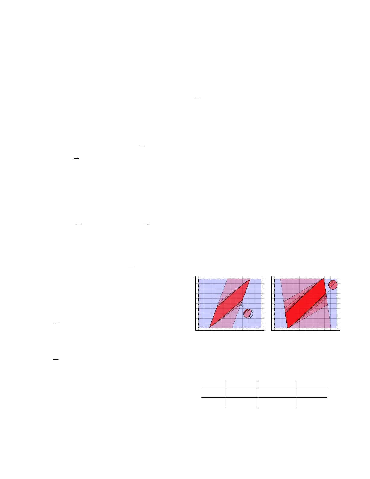
On maximal positiv e in v ar iant set computation f or r ank-deficient linear systems Bogdan Gheorghe, Daniel Ioan, Cristian Flutur Ionela Prodan, and Florin Stoican Abstract — The maximal positively in variant (MPI) set is obtained through a bac kward reachability procedure in volv- ing the iterative computation and intersection of predeces- sor sets under state and input constraints. Howe ver , standar d static feedbac k synthesis may place some of the closed-loop eigen values at zero, leading to rank-deficient dynamics. This affects the MPI computation by inducing projections onto lo wer-dimensional subspaces during intermediate steps. By exploiting the Schur decom- position, we explicitl y address this singular case and pro- pose a rob ust algorithm that computes the MPI set in both polyhedral and constrained-zonotope representations. Index T erms — maximal positive in variant set, con- strained zonotope, rank-deficient linear systems. I . I N T R O D U C T I O N The computation reachable sets is a fundamental problem at the intersection of control theory , algebraic geometry , and con vex optimization, serving to define the exact theoretical bounds for safe system operation [1], [2]. As a cornerstone of modern constrained control, reachability theory provides the mathematical guarantees necessary for recursiv e feasibility [3] and stability in Model Predictiv e Control (MPC) [4] applica- tions across the aerospace, chemical, and robotics sectors. A prime example of reachable set is the Maximal Positive In variant (MPI) set which denotes the largest positive in variant set which also respects feasibility constraints. It is computed via a set recurrence relation in volving the iterative calcula- tion and intersection of predecessor sets subject to state and input constraints. Its primary use is a terminal set in Model Predictiv e Control [4]. MPC operates by iterativ ely solving a finite-horizon optimization problem at each sampling interval, applying only the initial control action before receding the prediction horizon. A primary vulnerability is the potential loss of recursive feasibility: an optimal state sequence calculated at time k may dri ve the plant to a state at k + 1 from which future constraint violations become unav oidable. T o prev ent this and ensure closed-loop stability and constraint admissibility beyond the prediction horizon, the MPC formulation typically Bogdan Gheorghe, Daniel Ioan, Cristian Flutur , and Florin Stoican are with F aculty of Automation Control and Computer Science , National University of Science and T echnology Politehnica Bucharest, Romania { bogdan.gheorghe1807, daniel_mihail.ioan, cristian.flutur, florin.stoican } @upb.ro Ionela Prodan is with the Univ . Grenoble Alpes, Greno- ble INP † , LCIS, F-26000, V alence, F rance, † Institute of Engineer ing and Management Univ . Grenoble Alpes. ionela.prodan@lcis.grenoble-inp.fr forces the terminal state into an MPI set where the control action switches to a fixed terminal feedback law . The feedback gain K for this terminal law is usually com- puted via the resolution of a discrete-time algebraic Riccati equation. This unconstrained optimal design frequently results in placing one or more closed-loop eigen v alues at the origin ( 0 ). While mathematically optimal, this renders the result- ing closed-loop state transition matrix rank-deficient, which presents significant geometric and computational challenges for calculating the required terminal MPI set. While the MPI remains full-dimensional it is the result of computations where the singular closed-loop matrix maps the system dynamics into a lower -dimensional subspace, fundamentally altering the structural properties of the intermediate sets generated during this recurrence sequence. While established methodologies can compute these in vari- ant sets for standard polyhedral constraints, current literature lacks efficient solutions for the severe computational burdens introduced by the set recurrence at high dimensions. T o mitigate these, our recent work [5] has leveraged constrained zonotopes. By adding algebraic equality constraints, these structures retain efficient linear operations while remaining closed under arbitrary intersections. This allows the exact MPI set recurrence to be executed entirely within the constrained zonotope frame work. Our idea is straightforward but, to the best of our knowl- edge, was nev er treated in the literature: i) exploit the Schur factorization of the closed-loop ma- trix to identify the sub-space corresponding to non-zero eigen values and compute the reduced MPI set; ii) lift the reduced MPI back into the original space and intersect it with “initial constraints” to output the MPI set w .r .t. the original dynamics and feasible set. The remainder of this paper is organized as follows. Sec- tion II provides the preliminary mathematical background on MPI sets and their geometrical representations. Section III introduces the problem and provides theoretical justification for rank-deficient closed loop systems. Section IV details the MPI-computing procedure in both the polyhedral and constrained zonotopic representations. Section V provides illustrativ e examples, while Section VI draws the conclusions. Notations : F or a x ∈ R n , its infinity norm as ∥ x ∥ ∞ := max( | x 1 | , | x 2 | , . . . , | x n | ) . For A ∈ R n × n , eig ( A ) is the set of all its eigen values. I n ∈ R n × n is the identity matrix, and 1 n is the column vector of n values of one I I . P R E L I M I N A R I E S Consider the linear time-inv ariant system x k +1 = Ax k + B u k , (1) where x k , x k +1 ∈ R n denote the current and successor states; u k ∈ R m represents the input; A ∈ R n × n , B ∈ R n × m are the state and input matrices. The sets X ⊂ R n and U ⊂ R m impose constraints on the system state and input, respectiv ely . Assuming the pair ( A, B ) stabilizable, there exists a static gain K ∈ R m × n defining the feedback la w u k = K x k , which leads to the closed-loop matrix A ◦ := A + B K that stabilizes the system. The resulting closed-loop dynamics of (1) become x k +1 = A ◦ x k . (2) Furthermore, the open-loop constraints x k ∈ X and u k ∈ U imply the closed-loop state constraint x k ∈ X with X = X ∩ { x : K x ∈ U } . (3) A popular tool in the arsenal of set-based methods is the so-called maximal positively in variant (MPI) set [6], [7]. It is often used to define the terminal set in model predictiv e control architectures [4], ensuring recursiv e feasibility since it is, by definition, safe (due to positiv e in variance) and non- conservati ve (the “maximal” property). F or our purposes, it suffices to recall the standard set recurrence that computes it: Ω 0 = X , Ω k +1 = A − 1 ◦ Ω k ∩ X . (4) Under mild assumptions [8, Thm. 3], the recurrence (4) is guaranteed to terminate at a fix ed point Φ x := Ω ¯ k = Ω ¯ k +1 for some finite index ¯ k . Thus, an equiv alent form to (4) is Φ x = ¯ k \ k =0  x : A k ◦ x ∈ X  . (5) Further insights and variations of the basic MPI construction can be found in [9], [10] and subsequent works. Set descr iptions While the recurrence (4) is agnostic with respect to the nature of X , particular choices do influence the subsequent computations. A traditional option is the polyhedral represen- tation [11]. Writing X = { F X x ≤ θ X } , U = { F U u ≤ θ U } in their half-space form allows to express (3) as X := { F x ≤ θ } =  F X F U K  x ≤  θ X θ U  , (6) allows the recurrence (4) to be written explicitly as Φ x = ¯ k \ k =0  x : F A k ◦ x ≤ θ  . (7) An alternativ e representation is that of the constrained zonotope (CZ), first introduced in [12] and increasingly used for set manipulations [13]. W e call the compact set C Z ⊂ R n a constrained zonotope if there exists c ∈ R n , G ∈ R n × D , F ∈ R p × D , θ ∈ R p such that C Z =  c, G, F , θ  =  x = c + Gλ, F λ = θ , ∥ λ ∥ ∞ ≤ 1  . (8) Notew orthy , CZs are closed under set intersection [12]: C Z 1 ∩ C Z 2 = * c 1 ,  G 1 0  ,   F 1 0 0 F 2 G 1 − G 2   ,   θ 1 θ 2 c 2 − c 1   + . (9) Considering the state and input constraint sets as constrained zonotopes 1 X = ⟨ c X , G X , [ ] , [ ] ⟩ , U = ⟨ c U , G U , [ ] , [ ] ⟩ , allows, via (9), the set (3) to be expressed 2 as a CZ: X = ⟨ c, G, F , θ ⟩ =  c,  G 0  ,  K G − G U  , c U − K c  . (10) Based on [5], all sets Ω k = ⟨ c k , G k , F k , θ k ⟩ in the recurrence (4) are also CZs and can be computed recursively as Ω k +1 = D A − 1 ◦ c k ,  A − 1 ◦ G k 0  ,   F k 0 0 F A − 1 ◦ G k − G   ,   θ k θ c − A − 1 ◦ c k   E . (11) Illustrativ e example W e take the discrete in v ariant linear dynamics defined by: A =  1 . 38 0 . 76 0 . 16 1 . 87  , B =  1 1  with input and state constraints given by X = {∥ x ∥ ∞ ≤ 1 } , U = {∥ u ∥ ∞ ≤ 1 } . T ypically , closing the loop can be done either by solving the algebraic Riccati equation or by doing explicit pole placement. Each returns a stabilizing static gain K . Computing the MPI for dynamics (2) and feasible set (3) for each gain K results in the iterations illustrated in Figure 1. T able I shows that, ev en for this proof-of-concept e xample, − 1 − 0 . 8 − 0 . 6 − 0 . 4 − 0 . 2 0 0 . 2 0 . 4 0 . 6 0 . 8 1 − 1 − 0 . 8 − 0 . 6 − 0 . 4 − 0 . 2 0 0 . 2 0 . 4 0 . 6 0 . 8 1 X Ω 0 Ω 1 Ω 3 − 1 − 0 . 8 − 0 . 6 − 0 . 4 − 0 . 2 0 0 . 2 0 . 4 0 . 6 0 . 8 1 − 1 − 0 . 8 − 0 . 6 − 0 . 4 − 0 . 2 0 0 . 2 0 . 4 0 . 6 0 . 8 1 X Ω 0 Ω 1 Ω 3 (a) MPI set for Ricatti − 1 − 0 . 8 − 0 . 6 − 0 . 4 − 0 . 2 0 0 . 2 0 . 4 0 . 6 0 . 8 1 − 1 − 0 . 8 − 0 . 6 − 0 . 4 − 0 . 2 0 0 . 2 0 . 4 0 . 6 0 . 8 1 X Ω 0 Ω 1 Ω 2 Ω 3 Ω 7 − 1 − 0 . 8 − 0 . 6 − 0 . 4 − 0 . 2 0 0 . 2 0 . 4 0 . 6 0 . 8 1 − 1 − 0 . 8 − 0 . 6 − 0 . 4 − 0 . 2 0 0 . 2 0 . 4 0 . 6 0 . 8 1 X Ω 0 Ω 1 Ω 2 Ω 3 Ω 7 (b) MPI set for pole placement Fig. 1 : Example for computing the MPI set. significant differences appear in closed-loop in set shape and the v alue of ¯ k , the index where the recurrence stops. Method Poles Gain ( K ) Nr . of iter . ( k ) Ricatti h 0 . 48 0 . 83 i h 2 . 73 − 0 . 80 i 3 Placement h 0 . 95 0 . 7 i h 1 . 43 0 . 16 i 7 T ABLE I : Comparison of Ricatti and pole placement. 1 In many practical cases the constraint sets are h yperrectangles, and therefore equality constraints are not required in their definition. 2 W e abuse the notation and re-use F , θ for the equality part of the CZ description. I I I . P R O B L E M F O R M U L A T I O N A N D J U S T I FI C A T I O N The state matrix of the closed-loop dynamics (2) may possess multiple eigen v alues at λ = 0 (equi v alently , 0 ∈ eig( A ◦ ) ), possibly with dif ferent partial multiplicities. Such situations are not exceptional; rather , they naturally arise in a variety of standard control synthesis procedures. One such situation is optimal control, where the closed loop system may get poles placed anywhere in the unit disc, provided the stabilizing solution is computed [14]. W e recall that the stabilizing solution of the Riccati equation is computed as the disconjug ated in variant subspace of the Hamiltonian matrix, therefore the closed loop gain matrix K may place the eigen values of A + B K an ywhere in the stable region, so it may even place more than one eigen value at λ = 0 . Another situation of interest may result from a dead-beat control strategy [15], where all closed loop eigen values are placed at λ = 0 . Numerical example For illustration and later use in the paper , we consider the following numerical example, where the gain matrix K assigns parts of the closed loop spectrum to λ = 0 . Consider the controllable pair ( A, B ) and the feedback gain matrix K : A =       − 14 . 85 − 5 . 20 − 14 . 75 − 11 . 90 − 20 . 10 − 14 . 55 − 8 . 85 0 . 10 − 12 . 95 − 9 . 20 − 10 . 20 − 13 . 15 9 . 90 6 . 60 10 . 30 6 . 80 13 . 80 10 . 10 − 14 . 95 − 7 . 50 − 13 . 85 − 10 . 20 − 21 . 00 − 13 . 65 − 18 . 40 − 5 . 70 − 26 . 40 − 17 . 70 − 23 . 10 − 26 . 40 − 12 . 35 − 3 . 80 − 21 . 85 − 13 . 30 − 14 . 90 − 21 . 85       B =         1 4 3 4 0 0 0 2 4 4 4 2         , K =  1 0 4 2 1 4 3 1 2 2 4 2  . For the resulting closed loop matrix A ◦ = A + B K , we compute the Real Schur form matrix ( A ◦ = U S U ⊤ ). Matrix S =         0.70 -0.87 0.49 -0.31 35.16 -13.00 0 0.50 0.12 -0.23 2.27 -0.85 0 0 0.20 -0.40 -3.46 2.33 0 0 0 -0.00 -2.14 1.25 0 0 0 0.00 -0.00 -0.00 0 0 0 0 0 -0.00         has its eigenv alues at { 0 , 0 , 0 , 0 . 2 , 0 . 5 , 0 . 7 } . Furthermore, the eigen values at λ = 0 belong to two Jordan cells: one of dimension 1 and one of dimension 2 , [16, Chapter 3]. Such a simple example already rev eals the issue: either explicitly , as in (7), or implicitly , as in (11), we manipulate powers of the form A k ◦ = ( U S U ⊤ ) k = U S k U ⊤ . This becomes numerically unstable whenever S is singular , as is the case here. Therefore, the remainder of the paper exploits the structure of S to perform computations in a well- behav ed subspace, before lifting the results back to the original dimension. I V . M A I N I D E A In the singular case, matrix A ◦ is no longer full rank. Consequently , its image is not full dimensional. As a result, set recurrence (4) may behave erratically or fail altogether , since multiplication by A k ◦ effecti vely acts as a projection onto the subspace associated with nonzero poles. In the remainder of this section, we propose constructions that explicitly handle poles at zero, regardless of their nature, for both polyhedral and constrained-zonotope set descriptions. A. The polyhedral case W e handle first the case of polyhedral set descriptions (6)– (7), as shown in the following result. Pr oposition 1: Consider the singular closed-loop matrix A ◦ = A + B K = U  S 11 S 12 0 S 22  U ⊤ , (12) whose Schur decomposition has the (2 , 2) block S 22 ∈ R d 2 × d 2 nilpotent of degree p + 1 < n , i.e.,  S 22  p +1 = 0 , eig ( S 22 ) = 0 . (13) The scalars d 1 > 0 , d 2 > 0 satisfy d 1 + d 2 = n . Introducing the shorthand notation T = p X i =0  S 11  − i S 12  S 22  i , (14) the MPI set associated with the state matrix (12) and con- straints (6) is given by Φ x = Φ [1] x ∩ Φ [2] x , (15) with Φ [1] x = p − 1 \ k =0 X = p − 1 \ k =0  x : F A k ◦ x ≤ θ  , (16) Φ [2] x = ¯ k + p \ k = p X =  x : F z h  S 11  p  S 11  p − 1 T i U x ≤ θ z  . (17) The pair ( F z , θ z ) defines Φ z = ¯ k \ k =0 Z = { z : F z z ≤ θ z } , (18) the MPI set, computed as in (4), associated with the dynamics z + = S 11 z and constraint set Z = { z : F U 1 z ≤ θ } . U 1 gathers the first d 1 columns of U and U 2 the remaining d 2 columns. Pr oof: Under the Schur decomposition (12), the dy- namics (2) and the associated set X can be expressed in the transformed coordinates y = U ⊤ x , leading to y k +1 =  S 11 S 12 0 S 22  y k , (19a) Y = { y : F U y ≤ θ } . (19b) Both the dynamics and the associated constraint set follow from the change of variables x = U y together with the orthogonality property U U ⊤ = U ⊤ U = I . Decomposing y =  y ⊤ 1 y ⊤ 2  ⊤ we use (19a) to write the ev olution of each component of the state y 1 ,k +1 = S 11 y 1 ,k + S 12 y 2 ,k =  S 11  k +1 y 1 , 0 + k X i =0  S 11  k − i S 12  S 22  i y 2 , 0 , (20a) y 2 ,k +1 = S 22 y 2 ,k =  S 22  k +1 y 2 , 0 . (20b) Exploiting the nilpotence condition (13) we rewrite (20) into y 1 ,k +1 =  S 11  k +1 y 1 , 0 +  S 11  k min( k, p ) X i =0  S 11  − i S 12  S 22  i y 2 , 0 , (21a) y 2 ,k +1 = (  S 22  k +1 y 2 , 0 , k < p, 0 , k ≥ p. (21b) For con venience, let us denote z k = y 1 ,k + p and take T as in (14). Consequently , for any k ≥ p , (21a) is equi valently written as (we shift from k to k − p ) z k +1 = S 11 z k , z 0 =  S 11  p y 1 , 0 +  S 11  p − 1 T y 2 , 0 . (22) Using (21) in (19b) we observe a similar behavior for the constraints: for k ≥ p only the first component ( y 1 ,k ) is affected: Y = { F U y k ≤ θ } =  F  U 1 U 2   y 1 ,k y 2 ,k  ≤ θ  (21) = { F U 1 y 1 ,k ≤ θ } (22) = { F U 1 z k − p ≤ θ } . (23) At this point, we ha ve both ingredients required for the set recurrence (4): the dynamics given by the first part of (22) and the constraint set Z = { z : F U 1 z ≤ θ } . Applying the recurrence yields (18). Next, rewriting Φ z using the second part of (22) allo ws us to constrain explicitly y 1 , 0 and y 2 , 0 , obtaining (17) which enforces the constraints y k ∈ Y for all k ≥ p . By additionally imposing the constraints y k ∈ Y for k ≤ p , and reversing the change of coordinates x = U y , we obtain (16). Intersecting them gives (15), thus concluding the proof. B. Constr ained zonotopic case The same line of reasoning may be employed in the con- strained zonotopic case (11)–(11), as illustrated in the ne xt result. Pr oposition 2: Consider the notation from (12)–(14) and the constraint set giv en in its constrained zonotopic form X = ⟨ c, G, F , θ ⟩ , defined as in (10). Then the associated MPI set is given by Φ x =  c [1] ,  G [1] 0  ,    F [1] 0 0 F [2] h  S 11  p  S 11  p − 1 T i U ⊤ G [1] − G [2]    ,    θ [1] θ [2] c [2] − h  S 11  p  S 11  p − 1 T i c [1]     (24) where the “ [1] ” parameters describe the constraints imposed until k < p : Φ [1] x = p − 1 \ k =0 X =  c [1] , G [1] , F [1] , θ [1]  (25) and the “ [2] ” parameters describe the constraints applied to k ≥ p and, under dynamics (22) and set recurrence (11) which stops after ¯ k iterations [5]: Φ [2] x = ¯ k + p \ k = p X = { x : h  S 11  p  S 11  p − 1 T i U ⊤ x ∈ Φ z } , θ [2]  . (26) where Φ z = ¯ k \ k =0 Z = ⟨ c [2] , G [2] , F [2] , θ [2] ⟩ , (27) is the MPI set associated with the dynamics z + = S 11 z and constraint set Z =  U ⊤ 1 c, U ⊤ 1 G,  F U ⊤ 2 G  ,  θ − U ⊤ 2 c  . (28) All ( · ) [1] , ( · ) [2] parameters are obtained recursiv ely as in (11). Pr oof: Using recurrence (11) until step k = p − 1 for closed-loop matrix (12) and constraint set (10) gives Φ [1] x as in (25). Next, for k ≥ p , we consider the same change of coordinates as before, y = U ⊤ x . Using definition (8), we hav e that x k +1 ∈ X can be written as y 1 ,k +1 = U ⊤ 1 c + U ⊤ 1 Gλ k +1 , F 1 λ k +1 = θ 1 , (29a) y 2 ,k +1 = U ⊤ 2 c + U ⊤ 2 Gλ k +1 , F 2 λ k +1 = θ 2 . (29b) Due to (13) and as per (21b) we have that y 2 ,k +1 = 0 . This acts as an additional equality constraint on λ k +1 in (29b). Introducing it into (29a), leads to inclusion y 1 ,k +1 ∈ Z , with Z defined as in (28). W ith notation (22) and the set (28), set recurrence (11) leads to (27). Using the second part of (22) and (25) and (26) leads to (24), thus concluding the proof. C . Analysis Comparing Propositions 1 and 2, we observe that the same set names appear in both statements. This is not a mistake but a deliberate choice: the underlying geometric objects are identical. Indeed, constrained zonotopes and polyhedra ha ve been sho wn to be equiv alent set representations [13]. The differences arise only in the specific algorithms used to manip- ulate them (in this case, the operations of matrix multiplication and set intersection). T o emphasize this point, we present Algorithm (1), which enumerates the computation steps for both polyhedral and constrained-zonotope representations. Algorithm 1 MPI set for singular cases Input: A ◦ , X as in (6) or (8) Output: the MPI set Φ x 1 Compute the sorted real Schur form: A ◦ = U S U T with S and p + 1 as in (12) 2 Select procedure: Polyhedral Constrained Zonotope 3 Z from (23) Z from (28) 4 T ake A ◦ = S 11 , X = Z and compute reduced MPI set 5 Φ z as in (18) Φ z as in (27) 6 Compute auxiliary sets: 7 Φ [1] x from (16) Φ [1] x from (25) 8 Compute T as in (14) 9 Φ [2] x from (17) Φ [2] x from (26) 10 Compute MPI set Φ x = Φ [1] x T Φ [2] x Notew orthy , step 1 of the algorithm implements the or der ed Schur decomposition from [17], modified such that it arranges the Jordan and Schur blocks in descending order from largest to smallest, in magnitude. Thus, all the blocks with zero eigen value (if any) accumulate in the (2 , 2) block, as shown in (12). Sev eral remarks are in order . Remark 1: The set recurrence (4) terminates at some finite index ¯ k . Although unlikely , it is possible that ¯ k < p . In this case, the construction in (15) or (24) terminates without the need to compute (18) or (27) or , indeed, the parts of (16), (25) which correspond to indices ¯ k + 1 , . . . , p − 1 . ♦ Remark 2: Formulations (15) and (24) also provide geo- metric insight into why a singular matrix disrupts the standard recurrence (4). The set Φ z is computed in R d 1 . When embed- ded into R n as Φ [2] x after the change of v ariable y = U ⊤ x , it becomes unbounded along the subspace R d 2 . Consequently , the bounds that ensure a well-behav ed set must arise explicitly from the first p iterations, as collected in (16) and (25), respectiv ely . ♦ Remark 3: Index p + 1 , as defined in (13), corresponds to the dimension of the largest Jordan cell of S 22 . Inspecting the Jordan indices through the Schur form of S 22 , [18], provides additional insight into the nature of the constraints that arise at a given time instant k . For illustration, suppose that the block dimensions belong to the (not necessarily unique) ordered set { p 1 ≤ p 2 ≤ . . . ≤ p m } , with multiplicities { j 1 , j 2 , . . . , j m } . Then, for indices satisfying p i < k ≤ p i +1 , the constraints applied at step k (i.e., A k x ∈ X ) describe a geometric object embedded in a subspace of dimension n − P i ℓ =1 p ℓ j ℓ . Once k ≥ p = max ℓ =1 ,...,m p ℓ , the corresponding subspace dimension reaches d 1 = n − d 2 = n − P m ℓ =1 p ℓ j ℓ . ♦ V . I L L U S T R A T I V E E X A M P L E The following results were obtained using MPT3 [19] and CasADi [20]. All computations were performed on a system running Ub untu 22.04, equipped with an AMD Ryzen 9 3900X 3.8 GHz CPU (12 cores, 24 threads) and 48 GB of RAM. The MA TLAB implementation corresponding to Prop. 1 is av ailable in the subdirectory /replan-public/maximal-positive- in variant-set/LCSS-2026 of the GitLab repository: https: //gitlab.com/replan/replan- public.git . A. Numerical example in R 6 W e recall the numerical example from Section III. T o this we attach state and input constraints X = { x ∈ R 6 : ∥ x ∥ ∞ ≤ 1 } , U = { u ∈ R 2 : ∥ u ∥ ∞ ≤ 1 } which correspond to X =  I 6 I 2 K  x ≤  1 6 1 2  , giv en as in (3). Since in S , the upper -triangular matrix for the Schur factorization of A ◦ , we hav e two Jordan blocks (of dimensions p 1 = 1 and p 2 = 2 ), we ha ve that the rank deficiency is d 2 = p 1 + p 2 = 3 and p = max( p 1 , p 2 ) = 2 . Consequently , d 1 = n − d 2 = 3 and S 11 is the 3 × 3 matrix S 11 =   0 . 70 − 0 . 87 0 . 49 0 0 . 50 0 . 12 0 0 0 . 20   . Correspondingly , we compute the set Z ⊂ R 3 as shown below (18). Ha ving both these elements we compute the reduced MPI set Φ z from (18) in k = 3 iterations, as depicted in Fig. 2. Fig. 2 : MPI set Φ z in R 3 . By selecting the blocks S 12 and S 22 from S we compute, as in (14): T =   − 0 . 30 33 . 06 − 11 . 76 − 0 . 22 2 . 23 − 0 . 82 − 0 . 39 0 . 76 − 0 . 15   which is used, as in (17) to obtain Φ [2] x ⊂ R 6 . Set Φ [1] x ⊂ R 6 is obtained with p = 3 iterations as in (16). Intersecting the two, we obtain the desired result, the MPI set Φ x , characterizing the original dynamics and constraints. T otal computation time for all operations was 0 . 4 seconds. B. The CSE example [21] The Coupled Spring Experiment (CSE) considers a vari- able number of masses interconnected through springs and dampers. The system state consists of the positions and velocities of all masses, while the inputs are two external forces applied at the ends of the chain. The continuous-time model is given by ˙ x =  0 I − M − 1 c K c − M − 1 c L c  | {z } A ∈ R 2 ℓ × 2 ℓ x +  0 M − 1 c D c  | {z } B ∈ R 2 ℓ × 2 u, (30) where M c = µI , L c = δ I , K c = k          1 − 1 · · · 0 0 − 1 − 2 . . . 0 0 . . . . . . . . . . . . . . . 0 0 . . . − 2 − 1 0 0 · · · − 1 1          , and D c =        1 0 0 0 . . . . . . 0 0 0 − 1        , with µ = 4 , δ = 1 , k = 1 . The system is discretized using forward Euler method with a sampling time of 1 sec. The state and input constraints are: X = { x ∈ R 2 ℓ : ∥ x ∥ ∞ ≤ 1 } , U = { u ∈ R 2 : ∥ u ∥ ∞ ≤ 1 } . By varying the number of masses through the parameter ℓ , the state dimension becomes 2 ℓ . The application of Algorithm 1 in the polyhedral branch (Prop. 1) to the CSE dynamics, closed using both pole placement (all eigenv alues in the unit disk) and a Riccati- based method (yielding a rank-deficient matrix), is illustrated in Fig. 3. 2 3 4 5 6 7 8 9 10 0 10 20 30 40 50 parameter ℓ num ber of iterations ¯ k 0 1 , 000 2 , 000 3 , 000 4 , 000 5 , 000 Time [sec] ¯ k standard ¯ k rank deficient time standard time rank deficien t Fig. 3 : Plot number of iterations and commutation time. W e observe that: • Starting from higher dimensions ( ℓ = 8 , corresponding to x ∈ R 16 ), the number of iterations required by the standard algorithm ( ¯ k ) increases significantly , whereas the increase is moderate for the rank-deficient method; • The computation time further highlights the effecti veness of the proposed approach: the standard method becomes considerably more expensiv e for ℓ ≥ 8 , while the rank- deficient method remains computationally efficient; • The number of inequalities ¯ q required to represent the resulting polyhedral MPI sets is also larger for the stan- dard approach (starting from ℓ = 5 ). For instance, for ℓ = 10 , the standard method yields ¯ q = 1496 inequalities, whereas the rank-deficient method reduces to ¯ q = 704 . The resulting MPIs sets are not geometrically the same. This outcome is expected because of the pole placement, which changes the initial set X (as sho wn in Fig. 1). V I . C O N C L U S I O N S W e have presented a robust algorithm for computing the MPI set in the presence of rank-deficient dynamics, using the Schur factorization. The approach accommodates multiple zero eigen values with arbitrary multiplicities, and provides the resulting MPI set in both polyhedral and constrained-zonotope representations. Future work will extend this framework to the more general Maximal Output Admissible Set (MOAS), where we anticipate employing an SVD-based factorization. R E F E R E N C E S [1] H. R. Ossareh and I. Kolmano vsky , “On Complexity Bounds for the Maximal Admissible Set of Linear Time-In variant Systems, ” IEEE T ransactions on Automatic Control , pp. 1–8, 2024. [2] A. Dey and S. Bhasin, “Computation of maximal admissible robust positiv e inv ariant sets for linear systems with parametric and additive uncertainties, ” IEEE Contr ol Systems Letters , vol. 8, pp. 1775–1780, 2024. [3] H. Chen and F . Allgower , “ A quasi-infinite horizon nonlinear model predictiv e control scheme with guaranteed stability , ” Automatica , v ol. 34, no. 10, pp. 1205–1217, 1998. [4] S. V . Rakovi ´ c and W . S. Levine, Handbook of model predictive contr ol . Springer , 2018. [5] B. Gheorghe, D.-M. Ioan, F . Stoican, and I. Prodan, “Computing the maximal positive inv ariant set for the constrained zonotopic case, ” IEEE Contr ol Systems Letters , vol. 8, 2024. [6] E. Gilbert and K. T an, “Linear systems with state and control constraints: the theory and application of maximal output admissible sets, ” IEEE T ran. on Automatic Control , vol. 36, no. 9, pp. 1008–1020, 1991. [7] I. Kolmano vsky and E. G. Gilbert, “Theory and computation of dis- turbance in variant sets for discrete-time linear systems, ” Mathematical Pr oblems in Engineering , vol. 4, no. 4, pp. 317–363, 1998. [8] S. V . Rakovi ´ c and S. Zhang, “The implicit maximal positiv ely in variant set, ” IEEE T ran. on Automatic Contr ol , vol. 68, no. 8, pp. 4738–4753, 2023. [9] F . Blanchini and S. Miani, Set-theoretic methods in control . Springer , 2008, vol. 78. [10] B. Houska, M. A. M ¨ uller , and M. E. V illanuev a, “Polyhedral control design: Theory and methods, ” Annual Reviews in Contr ol , vol. 60, p. 100992, 2025. [11] G. M. Ziegler, Lectur es on polytopes . Springer Science & Business Media, 2012, vol. 152. [12] J. K. Scott, D. M. Raimondo, G. R. Marseglia, and R. D. Braatz, “Constrained zonotopes: A new tool for set-based estimation and fault detection, ” Automatica , vol. 69, pp. 126–136, 2016. [13] V . Raghuraman and J. P . Koeln, “Set operations and order reductions for constrained zonotopes, ” Automatica , vol. 139, p. 110204, 2022. [14] V . Ionescu, C. Oara, and M. W eiss, “General matrix pencil techniques for the solution of algebraic riccati equations: a unified approach, ” IEEE T ransactions on Automatic Contr ol , vol. 42, no. 8, pp. 1085–1097, 1997. [15] P . V an Dooren, “Deadbeat control: A special inv erse eigen v alue prob- lem, ” BIT Numerical Mathematics , vol. 24, no. 4, pp. 681–699, 1984. [16] R. A. Horn and C. R. Johnson, Matrix analysis . Cambridge univ ersity press, 2012. [17] J. H. Brandts, “Matlab code for sorting real Schur forms, ” Numerical linear algebra with applications , vol. 9, no. 3, pp. 249–261, 2002. [18] V . Kublanovskaya, “Construction of a canonic basis for matrices and pencils of matrices, ” Journal of Soviet Mathematics , vol. 20, no. 2, pp. 1929–1942, 1982. [19] M. Herceg, M. Kv asnica, C. Jones, and M. Morari, “Multi-Parametric T oolbox 3.0, ” in Pr oc. of the European Control Conference , Z ¨ urich, Switzerland, July 17–19 2013, pp. 502–510. [20] J. A. Andersson, J. Gillis, G. Horn, J. B. Rawlings, and M. Diehl, “CasADi: a software frame work for nonlinear optimization and optimal control, ” Mathematical Pr ogramming Computation , v ol. 11, no. 1, pp. 1–36, 2019. [21] F . Leibfritz, “COMPleib: COnstrained Matrix–optimization Problem library – a collection of test examples for nonlinear semidefinite pro- grams, control system design and related problems. ” Department of Mathematics, Univ . Trier , Germany , T ech. Rep., 2006.