Atomic Trajectory Modeling with State Space Models for Biomolecular Dynamics
Understanding the dynamic behavior of biomolecules is fundamental to elucidating biological function and facilitating drug discovery. While Molecular Dynamics (MD) simulations provide a rigorous physical basis for studying these dynamics, they remain…
Authors: Liang Shi, Jiarui Lu, Junqi Liu
Atomic T rajectory Modeling with State Space Models f or Biomolecular Dynamics Liang Shi 1 2 Jiarui Lu 3 4 Junqi Liu 1 2 Chence Shi 2 Zhi Y ang 1 Jian T ang 2 3 5 6 Abstract Understanding the dynamic behavior of biomolecules is fundamental to elucidating bio- logical function and facilitating drug discovery . While Molecular Dynamics (MD) simulations provide a rigorous physical basis for studying these dynamics, they remain computationally expensi ve for long timescales. Conv ersely , recent deep generati ve models accelerate conformation generation b ut are typically either failing to model temporal relationship or built only for monomeric proteins. T o bridge this gap, we introduce A TMOS, a nov el generativ e framew ork based on State Space Models (SSM) designed to generate atom-lev el MD trajectories for biomolecular systems. A TMOS integrates a Pairformer -based state transition mechanism to capture long-range temporal dependencies, with a dif fusion-based module to decode trajectory frames in an autore gressiv e manner . A TMOS is trained across crystal structures from PDB and conformation trajectory from large-scale MD simulation datasets including mdCA TH and MISA TO. W e demonstrate that A TMOS achiev es state-of-the-art performance in generating con- formation trajectories for both protein monomers and complex protein-ligand systems. By enabling ef ficient inference of atomic trajectory of motions, this work establishes a promising foundation for modeling biomolecular dynamics. 1. Introduction Elucidating the functional mechanisms of biomolecules re- quires a comprehensiv e understanding of protein dynamics, rather than merely analyzing static crystal structures. Tra- ditionally , Molecular Dynamics (MD) simulations are the 1 School of Computer Science, Peking Univ ersity 2 BioGeometry 3 Mila - Qu ´ ebec AI Institute 4 Univ ersit ´ e de Montr ´ eal 5 HEC Montr ´ eal 6 CIF AR AI Chair. Correspondence to: Zhi Y ang < yangzhi@pku.edu.cn > , Jian T ang < jian.tang@hec.ca > . Pr eprint. Mar ch 19, 2026. gold standard for this task, relying on fundamental physical principles to rev eal critical thermodynamic and kinetic prop- erties. Howe ver , despite rigorous adherence to physical laws, traditional MD methods are computationally expensi ve, of- ten struggling to access biologically rele vant timescales or sample rare conformational transitions efficiently . T o alle viate these computational burdens, recent research has pi voted to ward deep generati ve models. Broadly , these approaches fall into two categories. The first focuses on ensemble generation, where models like AlphaFlo w ( Jing et al. , 2024a ) and BioEmu ( Lewis et al. , 2025 ) emulate the equilibrium Boltzmann distribution. Howe ver , they typi- cally generate samples in an independent and identically dis- tributed ( i.i.d. ) manner , and fail to re veal kinetic pathways by discarding temporal correlations. The second category at- tempts generati ve trajectory modeling, represented by recent works such as MDGen ( Jing et al. , 2024b ), ConfRover ( Shen et al. , 2025 ), and TEMPO ( Xu et al. , 2025b ). While these methods begin to tak e the time dimension into consideration, they cannot model comple x systems of biomolecules. Addressing the aforementioned limitation, we introduce A tomic T rajectory MO deling with S SMs ( A TMOS ), which formulates biomolecular dynamics generation as a sequence modeling problem. A TMOS le verages State Space Models (SSM) to ef ficiently capture long-horizon trajectory e volu- tion with linear computational complexity in terms of the trajectory length. T o ensure geometric modeling capacity during temporal propagation, we parameterize the SSM state transition function using an adapted P airformer mod- ule ( Abramson et al. , 2024 ), ef fecti vely modeling geometric interactions within the latent evolution. Critically , unlike previous practices, this frame work operates on a atom-le vel coordinate representation by encoding states and decoding predicted trajectories without coarse-graining, thereby pre- serving detailed geometric contexts. The training data of A T - MOS comprises static structural data from the Protein Data Bank (PDB) and lar ge-scale MD simulation data from md- CA TH ( Mirarchi et al. , 2024 ) and MISA TO ( Siebenmor gen et al. , 2024 ). Experimental results demonstrates that the pro- posed A TMOS effecti vely models high-quality biomolecular dynamics, achie ving state-of-the-art performance in generat- ing conformation trajectories on both protein monomer and 1 Atomic T rajectory Modeling with State Space Models for Biomolecular Dynamics protein-ligand benchmarks. Our contributions to the field are summarized as follows: • W e present a unified generative framework for simu- lating dynamics of biomolecules, generalizing from monomeric proteins to complex biomolecular systems. • A TMOS models dynamics at the fully atomic le vel by operating directly on atomic coordinates during both the encoding and decoding phases, rather than coarse- graining representations like C α atoms or backbone frames. • W e innov ativ ely adapt State Space Models to the tra- jectory generation, enabling the capture of long-range temporal dependencies with improved inference ef fi- ciency compared to traditional simulation or purely attention-based approaches. • A TMOS demonstrates SO T A performance in generat- ing trajectories on large-scale MD datasets, specifically mdCA TH and MISA TO, v alidating the model’ s ability to generalize across div erse biological systems. • By successfully bridging static structural priors with dynamic trajectory generation, A TMOS extends the static structure prediction into the dynamics domain, paving the w ay tow ards dynamics foundation models. 2. Related W ork Generative Modeling of Pr otein Ensembles. Early data- driv en approaches for exploring protein conformational landscapes focused on modifying inputs to high-accuracy single-structure predictors. Methods such as MSA sub- sampling ( Del Alamo et al. , 2022 ; W ayment-Steele et al. , 2024 ) perturb the multiple sequence alignment fed into Al- phaFold2 to re veal alternati ve states, though these inference- time interventions often lack conformation div ersity ( Jing et al. , 2024a ). T o directly model equilibrium distrib utions, deep generativ e models have been dev eloped to sample conformations i.i.d. . Seminal work such as Boltzmann Generators ( No ´ e et al. , 2019 ) utilized normalizing flo ws to sample from the Boltzmann distrib ution, though scaling to systems beyond training remained challenging. Recent advances lev erage diffusion and flow matching on large- scale MD datasets; for instance, AlphaFlo w ( Jing et al. , 2024a ) fine-tunes pre-trained folding models to capture en- semble di versity , while EB A ( Lu et al. , 2025a ) enhances this framew ork with physical energy-based alignment. Other approaches focus on specific physical constraints or data regimes: Distrib utional Graphormer (DiG) ( Zheng et al. , 2024 ) and ConfDiff ( W ang et al. , 2024 ) incorporate energy or force guidance to improv e physical v alidity , Str2Str ( Lu et al. , 2024a ) employs a zero-shot translation framework without reliance on MD training data, ESMDif f ( Lu et al. , 2025b ) adopts latent language modeling to ef ficiently sam- ple conformation ensembles, and BioEmu ( Lewis et al. , 2025 ) integrates e xperimental stability data to predict ther- modynamic properties. Generative Modeling of Molecular T rajectories. While ensemble models capture time-independent distributions, trajectory generation methods aim to emulate the temporal ev olution of molecular systems, serving as surrogates for expensi ve Molecular Dynamics (MD) simulations. Initial ef- forts, such as ITO ( Schreiner et al. , 2023 ), T imeW arp ( Klein et al. , 2023 ) and EquiJump ( Costa et al. , 2024 ), focused on learning time-coarsened transition operators to jump ov er large time steps. More recent frame works model the joint distribution of entire trajectories to capture long-range temporal dependencies. MDGen ( Jing et al. , 2024b ) treats trajectories as time-series of 3D structures, utilizing flow matching to enable forward simulation, transition path inter - polation, and upsampling. T o handle the multi-scale nature of protein motions, TEMPO ( Xu et al. , 2025b ) introduces a hierarchical trajectory generation frame work that separates slow collectiv e motions from fast local fluctuations. Simi- larly , ConfRover ( Shen et al. , 2025 ) employs a causal trans- former with an SE(3) dif fusion decoder to simultaneously learn conformational distributions and dynamics. Other spe- cialized architectures include BioMD ( Feng et al. , 2025 ) for protein-ligand unbinding pathways, and PT raj-Diff ( Xu et al. , 2025a ) for protein-protein complex dynamics. 3. Method 3.1. Preliminaries Problem F ormulation. W e conceptualize the generation of biomolecular trajectory as a conditional sequence modeling task. Consider a biomolecular system consisting of N atoms. W e represent the dynamic e volution of this system as a tra- jectory of coordinates X = ( x 1 , x 2 , . . . , x T ) ∈ R T × N × 3 , where x t ∈ R N × 3 denotes the 3D Cartesian coordinates of all N atoms at time step t , and T represents the trajectory length, i.e., the number of frames. In addition to coordinates, the system is defined by time-in variant atomic features a , where a ∈ R N × d a represents atom-lev el attributes includ- ing atom type, residue type, molecule-le vel identifiers that indicate whether an atom belongs to a protein or ligand, etc. Our objectiv e is to learn a generativ e model p θ that approx- imates the true distribution of trajectories giv en the initial conformation x 1 and the context a . Follo wing standard autoregressi ve practices, we factorize the joint probability ov er the temporal dimension: p θ ( X | x 1 , a ) = T − 1 Y t =1 p θ ( x t +1 | x 1: t , a ) (1) 2 Atomic T rajectory Modeling with State Space Models for Biomolecular Dynamics Input Signal Geometric Encoder Transition Module Output Signal State Transition Encoding Structure Decoding Gaussian Prior Denoising Network Chemical Context All-atom Coordinate Token Distance Frame Orientation Chemical Context F igur e 1. Over view of the Proposed Atomic T rajectory Modeling Framework. This formulation allows the model to generate physically consistent long-horizon dynamics by conditioning the next state on the history of the trajectory and the chemical identity of the system. State Space Models (SSM). State Space Models ( Gu et al. , 2021a ; b ) provide a unified frame work for modeling se- quential data by mapping a 1-dimensional input signal u ( t ) ∈ R to an output signal y ( t ) ∈ R through a latent state h ( t ) ∈ R D . In their continuous-time form, linear SSMs are defined by the following ordinary dif ferential equations (ODEs): ˙ h ( t ) = A h ( t ) + B u ( t ) , y ( t ) = C h ( t ) (2) where A ∈ R D × D , B ∈ R D × 1 , and C ∈ R 1 × D are learn- able projection matrices. T o apply this framework to discrete sequence data (such as MD trajectories sampled at fixed in- tervals ∆ ), the continuous system is discretized—typically via the Zero-Order Hold (ZOH) method—yielding the re- currence: h t = A h t − 1 + B u t , y t = C h t (3) Here, A and B are the discretized state parameters. This recurrent formulation allows for efficient O (1) inference per step, making SSM particularly well-suited for generat- ing long molecular trajectories compared to the quadratic complexity of standard attention mechanisms. Notations. Throughout this paper , we use bold lo wercase letters (e.g., x , h ) for v ectors and atom-le v el representations, and bold or calligraphic uppercase letters (e.g., A , Φ , E ) for matrices and operations. W e denote the coordinate of the i -th atom at time t as x t,i ∈ R 3 . The set of all atoms is index ed by i ∈ { 1 , . . . , N } , and discrete time steps are index ed by t ∈ { 1 , . . . , T } . 3.2. An Atomic T rajectory Modeling Framework SSM as Learnable Biomolecular Simulators. W e frame the generation of biomolecular trajectories as the learning of a time-continuous ev olution function, functionally analo- gous to the integrator used in classical MD simulations. In traditional MD simulations, the system e v olves according to an inte grator that e xplicitly calculates future positions based on current coordinates, momenta, and inter-atomic forces deriv ed from a force field. While rigorous, this process is computationally intensiv e for long timescales. T o o vercome this, A TMOS adopts SSM as ef ficient, learn- able biomolecular propagators. Unlike standard attention- based sequence models that must revisit the entire history for ev ery prediction, SSM maintains a latent recurrent state. This aligns with the physical reality of molecular dynamics, which is inherently Mark ovian: the future ev olution of a sys- tem is gov erned by its current phase-space state (positions and momenta) rather than its explicit history . By replacing the expensi ve numerical integrator with a neural SSM, we achiev e a framew ork that is both physically intuitive and computationally efficient for long-horizon generation. Specifications. Formally , we instantiate the SSM frame- work for atomic trajectory modeling by defining the input signal, latent state, and output prediction as follows: • Input Signal ( x t ): The time-varying input to the model is the configuration of the system at time t , rep- resented by the atomic coordinates x t ∈ R N × 3 . This serves as the observ able states of the sequence. • Latent State ( h t ): The recurrent hidden state h t acts as an implicit representation of the system’ s complete phase-space state. While the input x t provides only the geometric configuration, the latent state h t captures the auxiliary dynamic variables necessary for propagation. Intuitiv ely , h effecti vely encodes implicit momenta, acting forces, and the thermodynamic memory (e.g., thermostat states) required to gov ern the Langevin dy- namics of the system. • Output Signal ( x t +1 ): Conditioning on the updated latent h t +1 , the model operates autoregressi vely to predict the updated coordinates x t +1 ∈ R N × 3 for the subsequent time step. Learning Objective. This frame work provides two crit- 3 Atomic T rajectory Modeling with State Space Models for Biomolecular Dynamics ical advantages. First, the constant inference complexity of SSMs per step (in recurrent mode) allows A TMOS to generate trajectories of arbitrary length T with linear scal- ing, addressing the bottleneck of existing autoregressi ve methods. Second, the continuous-time formulation of SSMs naturally handles the temporal correlations inherent in phys- ical motion, smoothing the modeling of rare conformational transitions. Under this framework, A TMOS can be trained to maximize the likelihood of the ground-truth trajectory X giv en the chemical context a . The learning objectiv e is: L SSM = − T − 1 X t =1 log p θ ( x t +1 | h t , x t , a ) (4) where p θ is parameterized by the predicted shift in coordi- nates. 3.3. Model Architectur e Compact Coupled Latent Representation. While our framew ork operates on full atomic coordinates to ensure precise dynamics, modeling interactions at the all-atom scale for lar ge biomolecular systems is computationally pro- hibitiv e. T o reconcile resolution with efficienc y , we adopt a compact (partially coarse-grained) coupled latent widely used in modern structure prediction architectures ( Jumper et al. , 2021 ; Abramson et al. , 2024 ). Specifically , we define the latent SSM state h t as a coupled representation operating on a tokenized sequence of length L (where L ≤ N ): h t ≜ ( s t , z t ) . (5) Here, the system is tokenized such that atom-le vel repre- sentations of protein are grouped into residue-le vel latents, otherwise the atomic resolution is retained. Consequently , s t ∈ R L × d s denotes the single r epr esentation , capturing the state of each residue or ligand atom, and z t ∈ R L × L × d z denotes the pair r epr esentation , encoding the interactions between tokens. This coupled representation allo ws A T - MOS to ef ficiently model long-range dependencies within the computationally manageable latent space, while k eeping the observable state as fine-grained atomic coordinates ( N ). Neural SSM Parametrization. While classical SSMs rely on linear projections (Eq. 2 ), modeling complex molecular interactions requires high-capacity non-linear transitions. Based on the coupled latent space, one can effecti vely pa- rameterize the state evolution using neural networks. The architecture is composed of three functional modules: Context and Input Encoding. W e first initialize the latent state by tokenizing the chemical conte xt a . An embedding layer maps contexts such as atom types and residue indices to the initial state h 0 ≜ ( s 0 , z 0 ) = e θ ( a ) , establishing the context prior of the system before dynamics begin. At each time step t , the input signal x t (current atomic coordinates) must be injected into the latent space to update the system’ s trajectory . W e employ a geometric encoder E θ to extract features from x t and fuses them with the static attributes a : v t = ( v s t , v z t ) = E θ ( x t , a ) (6) This term v t acts as the forcing term 1 (analogous to Bu t in Eq. 3 ), representing the instantaneous geometric update deriv ed from the current frame x t . State T ransition. The core propagator of A TMOS is the state transition function T θ , which ev olves the latent state h from t to t + 1 . W e instantiate this transition using a variant of the Pairformer module ( Abramson et al. , 2024 ), denoted as Φ θ : s , z 7→ s ′ , z ′ ∈ R L × d s , R L × L × d z . The Pairformer is uniquely suited for this role as it enables bidirectional information flo w between the single and pair tracks (Algo- rithm 2 ). The discretized update rule is defined as ( ∆ t > 0 indicates the time step): h t +1 ≜ ( s t +1 , z t +1 ) = T θ ( h t , v t , ∆ t ) . (7) Here, the transition kernel T θ is defined as T θ h t , v t , ∆ t ) ≜ T θ s t , z t ; v s t , v z t ; ∆ t ) = Φ θ s t + v s t + τ θ (∆ t ) , z t + v z t + τ θ (∆ t ) , (8) where τ θ ( · ) is broadcasted learnable timestep embeddings. Intuitiv ely , the Pairformer Φ θ functions as a learnable inte- grator , calculating the next latent state by reasoning ov er the previous memory h t and the current geometric update v t . Structur e Decoding. Finally , to map the ev olved latent state back to the coordinate space, we employ a dif fusion-based decoder . W e model the generation of the next frame x t +1 as a re verse dif fusion process. The core component is a denois- ing network D θ that predicts the clean, denoised structure from a noisy state. Specifically , for a giv en trajectory step t + 1 , we introduce a diffusion time v ariable γ ∈ [0 , + ∞ ] to distinguish the diffusion time from the trajectory inde x t . The decoder is conditioned on the noisy structure ˜ x ( γ ) , the chemical context a , and the e volv ed latent representations ( h t +1 ) . The denoising operation is defined as: ˆ x t +1 = D θ ( ˜ x ( γ ) , a , h t +1 , γ ) (9) where ˆ x t +1 represents the predicted denoised coordinates. By conditioning on the dual latent state ( s t +1 , z t +1 ) , the diffusion model is guided by both the detailed atomic state and the pairwise geometric constraints, ensuring the gener- ated structures are both chemically valid and dynamically consistent with the trajectory history . 1 Note that variables v s t ∈ R L × d s and v z t ∈ R L × L × d z are defined on the tok enized space and scale with the length L , whereas x t ∈ R N × 3 is defined in the raw coordinate space. 4 Atomic T rajectory Modeling with State Space Models for Biomolecular Dynamics 3.4. T raining Objectives T raining Regime. T o efficiently train A TMOS on long-horizon MD trajectory data, we employ a teacher- forcing ( W illiams & Zipser , 1989 ) with subsampling strat- egy during the training stage. Rather than unrolling the full trajectory , we optimize the model on sub-trajectory windows and input the prefix states as the ground truth. Specifically , for a gi ven training trajectory X = ( x 1 , . . . , x T ) of length T , we sample a start index t 0 , a temporal stride ∆ t , and a window size k such that 1 ≤ t 0 < t 0 + k ∆ t ≤ T . The model processes the first k − 1 frames as context to predict the target state x t 0 + k ∆ t at the strided k -th step. For sim- plicity , we adopt a fixed stride in this work, whereas we believ e it is worth exploring learn dynamics across v aried timescales by randomizing ∆ t . Loss Functions. As the learning objectiv e, we train A T - MOS end-to-end with tw o important loss terms: (1) latent fidelity loss (distogram) and (2) reconstruction loss (dif fu- sion), which are detailed as follows. Latent F idelity Loss (Distogr am). T o enforce geometric con- sistency in the latent space, we impose a distogram-based latent fidelity loss. Following Abramson et al. ( 2024 ), a lightweight prediction head P θ is applied to the pair repre- sentation z t , which outputs a 64 - bin probability distribution ov er discretized distances for each token pair ( i, j ) . The distogram loss is defined as the cross - entropy between the predicted distribution and the tar get bin (one-hot) deriv ed from the target coordinates: L disto = − E x t 1 L 2 L X i,j =1 64 X b =1 δ ( b ) ( i,j ) ( x t ) log P ( b ) θ, ( i,j ) ( z t, ( i,j ) ) , (10) where δ ( b ) ( i,j ) ( x t ) indicates whether the distance between tokens i and j in the target structure falls into the bin b , and the target frame x t is sampled via the training regime abo ve. Reconstruction Loss (Denoising Diffusion). This objectiv e optimizes the diffusion-based decoder D θ to (conditionally) recov er the target frame x t from a noise-corrupted state ˜ x ( γ ) . Firstly , we parameterize the decoder D θ using an EDM-style dif fusion process ( Karras et al. , 2022 ). During training, the noisy state is sampled follo wing the dif fusion time schedule γ ∼ p ( γ ) ∈ R + : ˜ x ( γ ) = x t + γ · ϵ, ϵ ∼ N (0 , I ) . (11) T o ensure the model focuses on non-trivial structural de via- tions rather than global rotations or translations, we apply the Kabsch algorithm to rigid align the target frame to the denoise coordinates. The loss is defined as: L recon = E x t ,γ ,ϵ " N X i =1 ω ( i, d, γ ) ∥ ˆ x i − Align ( x t,i ) ∥ 2 # (12) where ˆ x = D θ ( ˜ x ( γ ) , a , h t , γ ) is the predicted denoised structure. The weighting term ω ( i, d, γ ) = w entity ( i ) · w diff ( γ , σ data ) balances the loss by accounting for: atom entities w entity (distinguishes atoms from protein, ligand, etc.), dataset-specific noise scales σ data > 0 , and diffusion weighting w diff ( γ , σ data ) ≜ ( γ 2 + σ 2 data ) / ( γ · σ data ) 2 . The final training objectiv e is a linear combination as: L = λ recon · L recon + λ disto · L disto , (13) with λ recon > 0 , λ disto > 0 as tunable hyperparameters. 3.5. T rajectory Sampling Bi-Level Sampling Pr otocol. During inference, A TMOS samples trajectories in a specific temporal granularity ∆ t . Howe ver , autoregressi ve generation of high-dimension con- formation o ver long horizons can lose consistency due to ac- cumulated drift. Moti vated by prior work ( Henzler-W ildman & K ern , 2007 ; Xu et al. , 2025b ), we adopt a hierarchical, coarse-to-fine sampling strategy that decouples conforma- tion changes from local fluctuations. In practice, we special- ize two v ariants of A TMOS: a ke yframe gener ator G trained with a large temporal stride ( ∆ t kf ≜ u · ∆ t , where u > 1 is an upsampling factor) to predict distinct anchor confor - mations, and an interpolator I trained with a fine temporal stride ( ∆ t ) to fill in the dynamics between anchors; in other words, the interpolator upsamples (with the factor u > 1 ) the trajectory generated from G . This bi-level approach of- fers a key advantage: it enables the parallel generation of fine-grained frames between anchor frames and significantly enhances sampling efficienc y . Conditioned Interpolation. While the keyframe genera- tor operates via standard autoregressi ve rollout, the inter- polator requires awareness of the “destination” to ensure a coherent trajectory between endpoints, i.e., adjacent an- chor frames. Consequently , the interpolator variant I is conditioned on not only the starting frame x t , but also the subsequent anchor frame x t ′ (with t ′ = t + ∆ t kf ) and the remaining time horizon: p θ ( x t : t ′ | x t , x t ′ , a ) = Q u k =1 p θ ( x t + k ∆ t | x t : t +( k − 1)∆ t , x t ′ , a , t rem ) , where t rem ≡ ( u − k + 1)∆ t is the temporal distance between the current and the next anchor frame. 4. Experiments 4.1. Experimental Settings Dataset. W e ev aluate A TMOS on two modalities: single protein dynamics and protein-ligand dynamics. For protein dynamics, we adopt the mdCA TH dataset ( Mirarchi et al. , 2024 ), which provides molecular dynamics simulations for a wide range of protein domains. mdCA TH features simula- tions of 5,398 domains at fi ve different temperatures, each with fiv e replicas, of fering a large-scale, statistically robust 5 Atomic T rajectory Modeling with State Space Models for Biomolecular Dynamics T able 1. Evaluation on mdCA TH . The best scores are highlighted in bold and the second-best scores are underlined . r : Pearson correlation; J : Jaccard similarity; W 2 : 2-W asserstein distance. Conformation Models T rajectory Models Reference MD traj. AlphaFlow-MD ESMFlow-MD MDGen TEMPO ConfRover A TMOS Predicting flexibility Pairwise RMSD r ↑ 0.61 0.46 0.65 0.73 0.69 0.92 0.96 Global RMSF r ↑ 0.57 0.47 0.67 0.61 0.62 0.90 0.95 Per-tar get RMSF r ↑ 0.85 0.80 0.77 0.52 0.81 0.89 0.95 Distributional accuracy Root mean W 2 -dist. ↓ 3.40 5.00 3.86 4.98 4.52 2.70 1.89 MD PCA W 2 -dist. ↓ 2.26 2.16 2.75 2.38 3.04 1.79 1.67 Joint PCA W 2 -dist. ↓ 3.07 4.20 3.54 4.71 4.15 2.32 1.75 % PC-sim > 0 . 5 ↑ 35.5 25.8 3.17 7.94 22.2 47.6 61.9 Ensemble observables W eak contacts J ↑ 0.51 0.50 0.57 0.48 0.43 0.65 0.84 T ransient contacts J ↑ 0.29 0.26 0.22 0.20 0.22 0.38 0.55 T rajectory t-RMSD Error ↓ - - 2.71 2.42 2.50 1.79 0.00 perspectiv e on protein structural dynamics under varying conditions. The simulations are sampled at 1ns intervals. W e follow the dataset construction of TEMPO ( Xu et al. , 2025b ), which focuses on 320K trajectories and uses 1,000 domains for training, 50 for v alidation, and 64 for testing, with an av erage sequence similarity of 18.93% between the training and test sets, ensuring a challenging generalization benchmark. For protein–ligand dynamics, we use the MIS- A TO dataset ( Siebenmorgen et al. , 2024 ), which provides trajectories capturing the coupled dynamics of proteins and ligands. The simulations are performed at 300 K for 8 ns, yielding 100 snapshots per trajectory . W e preprocess MIS- A TO follo wing a procedure similar to Boltz - 2 ( P assaro et al. , 2025 ), resulting in 12,786 systems for training, 1,278 for val idation, and 1,289 for testing (see Appendix C for prepro- cessing details). Due to the computational cost of trajectory generation, we randomly sample 100 systems from the test set for final e valuation, aligning the test scale with Boltz - 2 and yielding final splits of 12,786 (train), 1,278 (val), and 100 (test). The PDB IDs of the sampled test systems are provided in Appendix C . Implementation details. W e initialize A TMOS with biomolecular structural priors by lev eraging pre - trained modules from Protenix ( Chen et al. , 2025 ), an open - source reproduction of AlphaF old3 ( Abramson et al. , 2024 ). Specif- ically , the context embedding layer that maps atom and residue attributes to the initial latent state h 0 ≜ ( s 0 , z 0 ) = e θ ( a ) , as well as the diffusion decoder D θ , are initialized with weights from Protenix. These modules provide an ef- fecti ve prior on plausible biomolecular geometries, enabling data - efficient learning of dynamics. The remaining com- ponents—the geometric encoder E θ and the state - transition kernel T θ —are trained from scratch. Architectural details of these modules are provided in the Appendix A . W e adopt the dual - scale generation strategy described in Section 3.5 . On the mdCA TH dataset, we train two separate models: one for coarse - scale keyframe generation at a 20ns interval and another for fine - scale interpolation at a 1ns interval. Similarly , for MISA TO, we train a coarse model at 0.8ns and a fine model at 0.08ns. This yields four trained models in total; we leave the e xploration of a unified model for future work. Complete training hyperparameter settings are listed in the Appendix D . 4.2. Protein Dynamics Baselines. W e compare A TMOS with three recent tra- jectory generation models: MDGEN ( Jing et al. , 2024b ), TEMPO ( Xu et al. , 2025b ), and ConfRov er ( Shen et al. , 2025 ). MDGEN and TEMPO are trained on mdCA TH, while for ConfRov er (which only provides inference code) we use the checkpoint trained on the A TLAS dataset ( V an- der Meersche et al. , 2024 ). Additionally , we include two SO T A conformation generation models, AlphaFlow - MD and ESMFlow - MD ( Jing et al. , 2024a ), which generate equilibrium ensembles without temporal correlations. Setup. For each protein in the test set, we condition on the initial structure and generate a trajectory of 400 frames at 1ns intervals, which we then compare to the corresponding MD reference trajectory . For the conformation generation baselines (AlphaFlo w - MD and ESMFlo w - MD), we gener - ate an independent set of conformations of equal size for comparison. Our ev aluation follows the protocol of Al- phaFlow ( Jing et al. , 2024a ), which assesses three aspects: flexibility prediction, distrib utional accuracy , and ensemble observables. Additionally , following TEMPO ( Xu et al. , 2025b ), we report the t-RMSD Error, a trajectory - lev el met- ric that quantifies a model’ s ability to reproduce the mag- nitude of conformational change o ver time. This metric is computed by (1) calculating the RMSD of each frame to the initial frame, and (2) computing the RMSE between the re- sulting RMSD sequences of the predicted and ground - truth trajectories. Detailed definitions and explanations of all metrics are provided in the Appendix E . Results. As sho wn in T able 1 , A TMOS achieves state-of-the- 6 Atomic T rajectory Modeling with State Space Models for Biomolecular Dynamics MD A TM O S A B t = 0 ns t = 2 0 ns t = 4 0 ns Ens em bles C D MD A TM O S F igur e 2. Case Study on 1s79a00 , a target from the test set of mdCA TH. (A) the visualization of ensemble from MD simulation (reference) or A TMOS (sampled). (B) The visualization of snapshot at specific frame index. (C) The RMSF versus the residue index. (D) The mo ving RMSD to the initial structure (frame 0) along the trajectory frames. art performance across all e valuation metrics, demonstrat- ing its ability to generate high-quality , physically realistic protein dynamics. On the flexibility prediction tasks, A T - MOS significantly outperforms both conformation models and pre vious trajectory models, achieving a near-perfect correlation with the reference MD trajectories in pairwise RMSD (Pearson r = 0 . 92 ) and global RMSF ( r = 0 . 90 ). This indicates that our model accurately captures both the ov erall conformational div ersity and the local atomic fluctu- ations present in real dynamics. In terms of distributional accuracy , A TMOS consistently produces ensembles that are closer to the reference distribution than any baseline, as evidenced by the lowest W asserstein distances across all three PCA-based metrics and the highest percentage of similar principal components (47.6%). Notably , it reduces the root mean 2 - W asserstein distance to 2.7 ˚ A, a substan- tial improv ement over the second - best conformation model (AlphaFlo w - MD, 3.40 ˚ A) and the best prior trajectory model (MDGEN, 3.86 ˚ A). This shows that A TMOS sample the cor- rect principal motion patterns. For ensemble observ ables, A TMOS also excels, achie ving the highest Jaccard similar- ity for both weak contacts and transient contacts, which are critical for understanding functional dynamics. Finally , on the trajectory - specific metric t-RMSD Error , A TMOS at- tains a value of 1.79 ˚ A, significantly lower than the best prior trajectory model. This result underscores the advantage of our state - space modeling approach in maintaining coherent, long-range temporal ev olution. Overall, the results v alidate that A TMOS successfully bridges the gap between static structural priors and dy- namic trajectory generation, offering a unified framework that captures both the equilibrium distribution and the ki- netic pathways of protein dynamics. W e further visualize one representativ e case in Figure 2 . T able 2. Efficiency evaluation on the 1gnla01 protein (139 AA). MD simulation is performed with Amber24 on GPU ( Salomon- Ferrer et al. , 2013 ), employing an integration time step of 4 fs. Model Inference T ime (Hour) Peak Mem (GB) MD Simulation > 10 < 1 ConfRov er 0.467 22.53 A TMOS 0.174 3.445 A TMOS-Parallel 0.044 6.117 Efficiency . W e e valuate the inference ef ficiency of A TMOS on the 1gnla01 protein (139AA) by generating a 400ns trajectory (400 frames at 1ns interv als). As shown in T a- ble 2 , A TMOS achie ves superior ef ficiency by le veraging state - space models, which capture long - range temporal de- pendencies with linear complexity in trajectory length. W e compare against two representativ e baselines: traditional MD simulation and ConfRover , which employs a causal transformer that must revisit the history for each prediction, leading to quadratic scaling. All methods are run on a sin- gle R TX 4090 GPU. A TMOS reduces inference time by 2.7 × compared to ConfRov er and by ov er 60 × compared to MD simulation, while using only 15% of ConfRov er’ s peak memory . By parallelizing the interpolation step across the batch dimension (A TMOS-Parallel), inference time is fur- ther reduced by 4 × at a modest increase in memory . These results validate that our SSM - based framework offers a com- pelling reduction in computational cost, enabling scalable generation of long, all-atom trajectories. 4.3. Protein-Ligand Dynamics Baselines. For protein-ligand dynamics, we compare with GNNMD ( Siebenmorgen et al. , 2024 ), DenoisingLD ( W u & Li , 2023 ), NeuralMD and V erletMD ( Liu et al. , 2025 ), DynamicBind ( Lu et al. , 2024b ), and Boltz-2 ( Passaro et al. , 7 Atomic T rajectory Modeling with State Space Models for Biomolecular Dynamics T able 3. Evaluation on MISA TO . The best scores are highlighted in bold and the second-best scores are underlined . r : Pearson correlation; W 2 : 2-W asserstein distance. Boltz - 2 is trained on the entire MISA TO dataset, which may lead to data leakage; we include it as a strong but potentially optimistic baseline. Method per-tar get RMSF r ↑ Root mean W 2 -dist ↓ Steric Clashes ↓ t-RMSD Error ↓ Ligand DenoisingLD ( W u & Li , 2023 ) 0.028 0.791 1.825 34.01 GNNMD ( Siebenmorgen et al. , 2024 ) 0.135 0.870 81.69 0.672 NeuralMD-SDE ( Liu et al. , 2025 ) 0.574 0.698 7.667 0.698 V erletMD ( Liu et al. , 2025 ) 0.456 36.83 14.67 43.78 DynamicBind ( Lu et al. , 2024b ) 0.678 1.470 7.113 - Boltz-2 ( Passaro et al. , 2025 ) 0.613 1.237 0.210 - A TMOS (ours) 0.746 0.670 0.030 0.480 Protein-Ligand DynamicBind ( Lu et al. , 2024b ) 0.193 2.288 52.74 - Boltz-2 ( Passaro et al. , 2025 ) 0.534 1.992 0.020 - A TMOS (ours) 0.523 1.567 0.051 0.600 2025 ). The first four models focus on ligand dynamics within the complex, while the latter two generate conforma- tional ensembles for the entire protein–ligand system. Setup. Similar to the ev aluation protocol for mdCA TH, we condition on the initial structure and generate the full trajectory . For the conformation generation baselines (Dy- namicBind and Boltz-2), we generate an independent set of conformations of equal size for comparison. W e as- sess four aspects: flexibility prediction (per - target RMSF Pearson correlation), distributional accuracy (root mean 2 - W asserstein distance), steric clashes, and trajectory ac- curacy (t-RMSD Error). Detailed metric definitions are provided in Appendix E . T wo important notes: (1) Since the first four baselines model only ligand dynamics, we re- port separate results for ligand-only and (where applicable) whole - system e valuations. (2) Boltz - 2 is trained on the en- tire MISA TO dataset, which may lead to data leakage; we include it as a strong but potentially optimistic baseline. Results. As shown in T able 3 , A TMOS achiev es strong performance across both lig and-only and full protein–ligand ev aluations. For ligand dynamics, A TMOS attains the best scores in all four metrics. These results demonstrate that our model generates physically realistic ligand motions while closely matching the reference distribution and temporal ev olution. On the full protein–ligand system, A TMOS de- liv ers competiti ve performance: it obtains the second - best RMSF correlation and clash count, while achieving the best W asserstein distance. Notably , A TMOS is the only method that reports an t-RMSD Error for the entire comple x, highlighting its ability to model coupled protein–ligand dy- namics with temporal coherence. Although Boltz - 2 sho ws slightly better performance on some metrics, it is trained on the entire dataset (potential data leakage) and does not produce trajectories, thus lacking any measure of temporal accuracy . In summary , A TMOS not only excels at model- ing ligand-in-pocket dynamics but also provides a unified framew ork for generating coherent, all - atom trajectories of the entire protein–ligand system. T able 4. Ablation study on sampling protocol . Metric A TMOS w/o bi-lev el sampling ODE Pairwise RMSD r ↑ 0.92 0.88 0.73 Global RMSF r ↑ 0.90 0.84 0.64 Per-tar get RMSF r ↑ 0.89 0.85 0.63 Root mean W 2 -dist. ↓ 2.70 3.06 3.89 MD PCA W 2 -dist. ↓ 1.79 2.09 2.73 Joint PCA W 2 -dist. ↓ 2.32 2.61 3.28 % PC-sim > 0 . 5 ↑ 47.6 39.1 17.2 W eak contacts J ↑ 0.65 0.56 0.26 T ransient contacts J ↑ 0.38 0.31 0.20 t-RMSD Error ↓ 1.79 2.03 3.22 4.4. Ablation Study W e ablate two ke y sampling configurations in A TMOS: the bi - le vel sampling protocol and the stochasticity of the EDM- based dif fusion sampling ( Karras et al. , 2022 ). Results on mdCA TH (T able 4 ) show that removing the hierarchical generation strate gy degrades performance across all metrics, confirming that generating coarse keyframes before interpo- lation reduces error accumulation and improves long - range consistency . Replacing the SDE (see Algorithm 4 ) with a de- terministic ODE flo w (see Appendix A.3 ) similarly causes a pronounced drop in ensemble quality . This demonstrates that stochastic diffusion is essential for capturing the thermal div ersity of biomolecular conformations. 5. Conclusion W e present A TMOS, a unified generative framew ork for simulating biomolecular dynamics that generalizes from monomeric proteins to complex biomolecular systems. A T - MOS operates at the all - atom le vel and adapts state - space models to trajectory generation, enabling efficient capture of long - range temporal dependencies with linear inference complexity . The model achieves SO T A performance on large - scale MD benchmarks, demonstrating its ability to generalize across div erse biological systems and paving the way to ward foundational dynamics models. 8 Atomic T rajectory Modeling with State Space Models for Biomolecular Dynamics Impact Statement A TMOS has significant broader impacts for computational biology and drug disco very . It provides a general - purpose framew ork for modeling biomolecular dynamics that could accelerate therapeutic discovery and enhance biological un- derstanding. Howe ver , ethical concerns, such as potential misuse in drug dev elopment, warrant careful consideration. Responsible deployment and transparency are essential to maximize benefits and mitigate risks. References Abramson, J., Adler, J., Dunger , J., Evans, R., Green, T ., Pritzel, A., Ronneberger , O., Willmore, L., Ballard, A. J., Bambrick, J., et al. Accurate structure prediction of biomolecular interactions with alphafold 3. Natur e , 630 (8016):493–500, 2024. Chen, X., Zhang, Y ., Lu, C., Ma, W ., Guan, J., Gong, C., Y ang, J., Zhang, H., Zhang, K., W u, S., et al. Protenix- advancing structure prediction through a comprehensi ve alphafold3 reproduction. bioRxiv , pp. 2025–01, 2025. Costa, A. D. S., Mitniko v , I., Pellegrini, F ., Daigav ane, A., Geiger , M., Cao, Z., Kreis, K., Smidt, T ., Kucukbenli, E., and Jacobson, J. Equijump: Protein dynamics simula- tion via so (3)-equi variant stochastic interpolants. arXiv pr eprint arXiv:2410.09667 , 2024. Del Alamo, D., Sala, D., Mchaourab, H. S., and Meiler , J. Sampling alternati ve conformational states of transporters and receptors with alphafold2. Elife , 11:e75751, 2022. Feng, B., Zhang, J., Zhang, X., Liu, Z., and Li, Y . Biomd: All-atom generati ve model for biomolecular dynamics simulation. arXiv preprint , 2025. Gu, A., Goel, K., and R ´ e, C. Efficiently modeling long sequences with structured state spaces. arXiv preprint arXiv:2111.00396 , 2021a. Gu, A., Johnson, I., Goel, K., Saab, K., Dao, T ., Rudra, A., and R ´ e, C. Combining recurrent, con volutional, and continuous-time models with linear state space layers. Advances in neur al information pr ocessing systems , 34: 572–585, 2021b. Henzler-W ildman, K. and Kern, D. Dynamic personalities of proteins. Nature , 450(7172):964–972, 2007. Jing, B., Berger , B., and Jaakkola, T . AlphaFold meets flow matching for generating protein ensembles. In Salakhutdinov , R., K olter , Z., Heller , K., W eller , A., Oliv er , N., Scarlett, J., and Berkenkamp, F . (eds.), Pr o- ceedings of the 41st International Confer ence on Ma- chine Learning , volume 235 of Pr oceedings of Ma- chine Learning Resear ch , pp. 22277–22303. PMLR, 21– 27 Jul 2024a. URL https://proceedings.mlr. press/v235/jing24a.html . Jing, B., St ¨ ark, H., Jaakkola, T ., and Berger , B. Generativ e modeling of molecular dynamics trajectories. Advances in Neural Information Pr ocessing Systems , 37:40534– 40564, 2024b. Jumper , J., Ev ans, R., Pritzel, A., Green, T ., Figurnov , M., Ronneberger , O., Tun yasuvunakool, K., Bates, R., ˇ Z ´ ıdek, A., Potapenko, A., et al. Highly accurate protein structure prediction with alphafold. natur e , 596(7873):583–589, 2021. Karras, T ., Aittala, M., Aila, T ., and Laine, S. Elucidating the design space of diffusion-based generative models. Advances in neur al information pr ocessing systems , 35: 26565–26577, 2022. Klein, L., Foong, A., Fjelde, T ., Mlodozeniec, B., Brockschmidt, M., No wozin, S., No ´ e, F ., and T omioka, R. Time warp: T ransferable acceleration of molecular dy- namics by learning time-coarsened dynamics. Advances in Neural Information Pr ocessing Systems , 36:52863– 52883, 2023. Lewis, S., Hempel, T ., Jim ´ enez-Luna, J., Gastegger , M., Xie, Y ., Foong, A. Y ., Satorras, V . G., Abdin, O., V eeling, B. S., Zaporozhets, I., et al. Scalable emulation of pro- tein equilibrium ensembles with generati ve deep learning. Science , 389(6761):eadv9817, 2025. Liu, S., Du, W ., Xu, H., Li, Y ., Li, Z., Bhethanabotla, V ., Y an, D., Borgs, C., Anandkumar , A., Guo, H., et al. A multi-grained symmetric dif ferential equation model for learning protein-ligand binding dynamics. Natur e Com- munications , 2025. Lu, J., Zhong, B., Zhang, Z., and T ang, J. Str2str: A score-based framew ork for zero-shot protein conforma- tion sampling. In The T welfth International Confer - ence on Learning Repr esentations , 2024a. URL https: //openreview.net/forum?id=C4BikKsgmK . Lu, J., Chen, X., Lu, S. Z., Lozano, A., Chenthamarak- shan, V ., Das, P ., and T ang, J. Aligning protein con- formation ensemble generation with physical feedback. In Singh, A., Fazel, M., Hsu, D., Lacoste-Julien, S., Berkenkamp, F ., Maharaj, T ., W agstaff, K., and Zhu, J. (eds.), Pr oceedings of the 42nd International Confer ence on Machine Learning , v olume 267 of Pr oceedings of Ma- chine Learning Resear ch , pp. 40436–40451. PMLR, 13– 19 Jul 2025a. URL https://proceedings.mlr. press/v267/lu25b.html . 9 Atomic T rajectory Modeling with State Space Models for Biomolecular Dynamics Lu, J., Chen, X., Lu, S. Z., Shi, C., Guo, H., Bengio, Y ., and T ang, J. Structure language models for protein conforma- tion generation. In The Thirteenth International Confer- ence on Learning Repr esentations , 2025b. URL https: //openreview.net/forum?id=OzUNDnpQyd . Lu, W ., Zhang, J., Huang, W ., Zhang, Z., Jia, X., W ang, Z., Shi, L., Li, C., W olynes, P . G., and Zheng, S. Dynam- icbind: predicting ligand-specific protein-ligand complex structure with a deep equi v ariant generati ve model. Na- tur e Communications , 15(1):1071, 2024b. McGibbon, R. T ., Beauchamp, K. A., Harrigan, M. P ., Klein, C., Swails, J. M., Hern ´ andez, C. X., Schwantes, C. R., W ang, L.-P ., Lane, T . J., and Pande, V . S. Mdtraj: a modern open library for the analysis of molecular dynam- ics trajectories. Biophysical journal , 109(8):1528–1532, 2015. Mirarchi, A., Giorgino, T ., and De Fabritiis, G. mdcath: A large-scale md dataset for data-driven computational biophysics. Scientific Data , 11(1):1299, 2024. No ´ e, F ., Olsson, S., K ¨ ohler , J., and W u, H. Boltzmann gener - ators: Sampling equilibrium states of man y-body systems with deep learning. Science , 365(6457):eaaw1147, 2019. Passaro, S., Corso, G., W ohlwend, J., Reveiz, M., Thaler, S., Somnath, V . R., Getz, N., Portnoi, T ., Roy , J., Stark, H., et al. Boltz-2: T o wards accurate and efficient binding affinity prediction. BioRxiv , 2025. Salomon-Ferrer , R., Gotz, A. W ., Poole, D., Le Grand, S., and W alker , R. C. Routine microsecond molecular dynam- ics simulations with amber on gpus. 2. explicit solvent particle mesh ewald. Journal of chemical theory and computation , 9(9):3878–3888, 2013. Schreiner , M., W inther , O., and Olsson, S. Implicit transfer operator learning: Multiple time-resolution models for molecular dynamics. Advances in Neural Information Pr ocessing Systems , 36:36449–36462, 2023. Shen, Y ., W ang, L., Y uan, H., W ang, Y ., Y ang, B., and Gu, Q. Simultaneous modeling of protein conformation and dynamics via autoregression. In ICML 2025 Generative AI and Biology (GenBio) W orkshop , 2025. URL https: //openreview.net/forum?id=BaZL1cQzV0 . Siebenmorgen, T ., Menezes, F ., Benassou, S., Merdi van, E., Didi, K., Mour ˜ ao, A. S. D., Kitel, R., Li ` o, P ., Kesselheim, S., Piraud, M., et al. Misato: machine learning dataset of protein–ligand complex es for structure-based drug dis- cov ery . Nature computational science , 4(5):367–378, 2024. V ander Meersche, Y ., Cretin, G., Gheeraert, A., Gelly , J.-C., and Galochkina, T . Atlas: protein flexibility description from atomistic molecular dynamics simulations. Nucleic acids r esear ch , 52(D1):D384–D392, 2024. W ang, Y ., W ang, L., Shen, Y ., W ang, Y ., Y uan, H., W u, Y ., and Gu, Q. Protein conformation generation via force-guided se (3) dif fusion models. arXiv preprint arXiv:2403.14088 , 2024. W ayment-Steele, H. K., Ojoawo, A., Otten, R., Apitz, J. M., Pitsaw ong, W ., H ¨ omberger , M., Ovchinnikov , S., Colwell, L., and K ern, D. Predicting multiple conformations via sequence clustering and alphafold2. Natur e , 625(7996): 832–839, 2024. W illiams, R. J. and Zipser, D. A learning algorithm for con- tinually running fully recurrent neural networks. Neural computation , 1(2):270–280, 1989. W u, F . and Li, S. Z. Diffmd: a geometric diffusion model for molecular dynamics simulations. In Proceedings of the AAAI confer ence on artificial intelligence , v olume 37, pp. 5321–5329, 2023. Xu, K., W ang, J., Liu, M., Zhou, K., Lin, S., Li, W ., Shi, L., Zhou, P ., Liu, H., and Y ao, X. Efficient generation of protein and protein–protein complex dynamics via se(3)- parameterized diffusion models. Journal of Chemical Information and Modeling , 65(22):12366–12376, 2025a. Xu, Y ., W ang, D., Zhou, Z., Y u, T ., and Chen, M. TEMPO: T emporal multi-scale autore gressiv e generation of protein conformational ensembles. In The Thirty-ninth Annual Confer ence on Neural Information Pr ocessing Systems , 2025b. URL https://openreview.net/forum? id=0wV5HR7M4P . Zheng, S., He, J., Liu, C., Shi, Y ., Lu, Z., Feng, W ., Ju, F ., W ang, J., Zhu, J., Min, Y ., et al. Predicting equilibrium distributions for molecular systems with deep learning. Natur e Machine Intellig ence , 6(5):558–567, 2024. 10 Atomic T rajectory Modeling with State Space Models for Biomolecular Dynamics A. Architectural Details This section provides implementation details for the ke y modules introduced in Section 3.3 . Input Signal Geometric Encoder Distogram Extractor Unit Vector Extractor Atom Attention Encoder Chemical Context Concat MLP Transition Module Pairformer Stack (BIF) Conditional Diffusion Module Denoising Network Gaussian Prior Output Signal F igur e 3. Detailed ar chitecture of our framework. BIF: Bidirectional Information Flow . A.1. Context and Input Encoding W e initialize the context embedding layer e θ with the pre - trained trunk module of Protenix ( Chen et al. , 2025 ) (an open - source reproduction of AlphaFold3 ( Abramson et al. , 2024 )), which includes the Input Feature Embedder, MSA Module and Pairformer . This module is fine-tuned during training. The geometric encoder E θ maps the current all - atom conformation X t into a forcing term v t = ( v s t , v z t ) that captures both global topology and local atomic details. Consistent with the dual - track latent representation, E θ decomposes structural information into a token - lev el single representation v s t ∈ R L × d s and a pairwise representation v z t ∈ R L × L × d z , where L denotes the length of the tokenized sequence. Pairwise geometric featur es. For each token pair ( i, j ) , we compute in varia nt features that encode their relative geometry . For protein residues, the tok en center is taken as the C β atom (C α for glycine); for ligand atoms, the atom itself serv es as the center . W e compute (1) a distance histogram between the two centers, and (2) unit vectors that express the displacement vector in the local coordinate frame of each token (constructed from backbone atoms for residues and neighboring atoms for ligands). These features are concatenated and projected: v z t [ i, j ] = MLP concat( Distogram ij , UnitV ectors ij ) . (14) T oken - wise local encoding. T o capture detailed side - chain conformations and local chemical en vironments, we employ an AtomAttentionEncoder (Algorithm 1 ) similar to the one in AlphaFold3 ( Abramson et al. , 2024 )). This module pro- cesses the current all - atom structure X t and summarizes intra - token atomic arrangements and their neighborhoods into a fixed-dimensional token-wise representation: v s t = A tomAtten tionEncoder X t , a . (15) Pseudocode for the AtomAttentionEncoder submodules (e.g., AtomTransformer) follo ws the description in the AlphaFold 3 supplementary material ( Abramson et al. , 2024 ). T ogether , v s t and v z t provide a comprehensiv e geometric encoding that serves as the forcing term to the state transition module. A.2. State T ransition The core propagator of A TMOS is the state transition function T θ , which evolv es the latent state h from t to t + 1 . W e instantiate T θ as a variant of the Pairformer module (Algorithm 2 ) ( Abramson et al. , 2024 ), which is uniquely suited for this role because it enables bidirectional information flow between the single and pair tracks. For reference, we provide the original Pairformer pseudocode in Algorithm 3 and highlight the modifications in Algorithm 2 . Pseudocode for the Pairformer submodules (e.g., T riangleMultiplicationOutgoing, TriangleAttentionStartingNode) follo ws the description in the AlphaFold 3 supplementary material ( Abramson et al. , 2024 ). W e use 4 Pairformer blocks in our implementation. The architectural hyperparameters are listed in T able 5 . 11 Atomic T rajectory Modeling with State Space Models for Biomolecular Dynamics Algorithm 1 Atom Attention Encoder 1: Input: all-atom coordinate x ∈ R N × 3 , Chemical Context a . 2: Output: forcing term v s ∈ R N × d s . 3: c i ← LinearNoBias ( concat ( x i , a atom charge i , a atom element i , a atom name i )) 4: d ij ← x i − x j 5: m ij ← 1 . 0 if atom i, j are located in the same token else 0 . 0 6: p ij ← LinearNoBias ( d ij ) · m ij 7: p ij ← p ij + LinearNoBias (1 / (1 + || d ij || 2 2 )) · m ij 8: p ij ← p ij + LinearNoBias ( m ij ) · m ij 9: p ij ← p ij + LinearNoBias ( ReLU ( c i )) + LinearNoBias ( ReLU ( c j )) 10: p ij ← p ij + MLP ( p ij ) 11: q ← AtomT ransformer ( q , p ) # Atom local attention; same architecture as AlphaF old 3; p is the pair bias. 12: v s ← mean pooling ( q ) # Pool atom-le vel representation into token-le vel representation. 13: Return v s T able 5. Architectural hyperparameters for the modified Pairformer . Hyperparameter V alue Number of Pairformer blocks 4 Single representation dimension 384 Pair representation dimension 128 T riangle multiplication hidden dimension 128 Number of triangle attention heads 4 T ransition layer expanding factor 4 Pair attention dropout rate 0.25 A.3. Structure Decoding W e model the generation of the next frame x t +1 as a re verse dif fusion process, with a denoising network D θ that predicts the clean structure from a noisy state. The diffusion decoder D θ is initialized from the weights of Protenix ( Chen et al. , 2025 ). T ogether with the context embedding layer e θ , this provides a strong prior on plausible biomolecular geometries, enabling data - efficient learning of dynamics. W e parameterize the decoder D θ using an EDM - style dif fusion process ( Karras et al. , 2022 ). The conditional diffusion sampling procedure is detailed in Algorithm 4 . W e use N step = 50 diffusion steps, a step scaling factor η = 1 . 5 , and a noise scaling schedule parameter γ 0 = 0 . 8 with a minimum γ min = 1 . 0 . The noise scaling factor λ is set to 1 . 5 for mdCA TH (to encourage div ersity) and 1 . 003 for MISA TO. Note that the stochastic differential equation (SDE) in Algorithm 4 can be con verted to a deterministic ordinary dif ferential equation (ODE) by setting γ 0 = 0 , as done in the ablation study . B. Inference W e detail the bi - lev el sampling protocol introduced in Section 3.5 . The procedure, summarized in Algorithm 5 , consists of two stages: (1) generating a sparse set of keyframes at a coarse time resolution, and (2) filling in the intermediate frames via parallel interpolation conditioned on the adjacent keyframes. In the keyframe generation stage (lines7 - 13), the model autoregressi v ely predicts a sequence of anchor conformations spaced by ∆ t kf = u ∆ t . Each step encodes the last generated frame, updates the latent state, and samples a new keyframe via diffusion. In the interpolation stage (lines15 - 30), for each pair of consecuti ve ke yframes ( x start , x end ) , we generate u − 1 intermediate frames at the fine resolution ∆ t . Crucially , the interpolator’ s transition function T θ is additionally conditioned on the encoded end frame ( v s end , v z end ) and the remaining time rem times , ensuring that the generated path remains coherent with the destination. This design allows all intermediate frames within an interv al to be generated in parallel, significantly accelerating sampling while maintaining trajectory consistency . 12 Atomic T rajectory Modeling with State Space Models for Biomolecular Dynamics Algorithm 2 PairformerStack with Bidirectional Information Flo w 1: Input: single representation s , pair representation z , pairformer block number N block 2: Output: updated single representation s , pair representation z . 3: for l ∈ [1 , . . . , N block ] do 4: { z ij } ← { z ij } + { s i } + { s j } 5: { z ij } ← { z ij } + DropoutRowwise 0 . 25 ( T riangleMultiplicationOutgoing ( { z ij } )) 6: { z ij } ← { z ij } + DropoutRowwise 0 . 25 ( T riangleMultiplicationIncoming ( { z ij } )) 7: { z ij } ← { z ij } + DropoutRowwise 0 . 25 ( T riangleAttentionStartingNode ( { z ij } )) 8: { z ij } ← { z ij } + DropoutColumnwise 0 . 25 ( T riangleAttentionEndingNode ( { z ij } )) 9: { z ij } ← { z ij } + Transition ( { z ij } ) 10: { s i } ← { s i } + AttentionPairBias ( { s i } , { z ij } ) 11: { s i } ← { s i } + Transition ( { s i } ) 12: end for 13: Return s , z Algorithm 3 Original AlphaFold P airformerStack 1: Input: single representation s , pair representation z , pairformer block number N block 2: Output: updated single representation s , pair representation z . 3: for l ∈ [1 , . . . , N block ] do 4: { z ij } ← { z ij } + DropoutRowwise 0 . 25 ( T riangleMultiplicationOutgoing ( { z ij } )) 5: { z ij } ← { z ij } + DropoutRowwise 0 . 25 ( T riangleMultiplicationIncoming ( { z ij } )) 6: { z ij } ← { z ij } + DropoutRowwise 0 . 25 ( T riangleAttentionStartingNode ( { z ij } )) 7: { z ij } ← { z ij } + DropoutColumnwise 0 . 25 ( T riangleAttentionEndingNode ( { z ij } )) 8: { z ij } ← { z ij } + Transition ( { z ij } ) 9: { s i } ← { s i } + AttentionPairBias ( { s i } , { z ij } ) 10: { s i } ← { s i } + Transition ( { s i } ) 11: end for 12: Return s , z C. MISA TO Dataset Pr eprocessing W e preprocess the MISA TO dataset following a procedure similar to Boltz - 2 ( Passaro et al. , 2025 ), resulting in 12,786 systems for training, 1,278 for validation, and 1,289 for testing. The preprocessing consists of se veral steps. First, we download the MD restart file (to e xtract bond topology) and the MD result file (which contains trajectory coordinates and can be used to infer chain ids). Next, we generate a (.prmtop, .nc) pair for each protein–ligand complex. The .prmtop file holds topology information and the .nc file stores the trajectory coordinates. These files are loaded with MDTraj ( McGibbon et al. , 2015 ), and each frame is exported as an individual PDB file. This method preserves complete topology (including bonds) and ensures a robust ligand representation, whereas directly constructing a PDB from the MD result file can lose atoms and introduce parsing inconsistencies. W e then add CCD (Chemical Component Dictionary) information to the loaded (.prmtop, .nc) pair, and con vert them to (.pdb, .xtc) format. Systems that do not contain a MOL (ligand) residue are excluded. W e also remove systems where the ligand’ s atomic elements differ from those in the corresponding PDBBind MOL2 files, ensuring chemical consistency . Additionally , trajectories in which the ligand drifts more than 12 ˚ A from the protein at any frame are filtered out. Furthermore, we remove approximately 500 systems that cannot be processed by the Protenix ( Chen et al. , 2025 ) data pipeline due to unexpected errors, indicating potential format, content, or geometry issues. (W e first con verts the PDB file to mmCIF format and then applies Protenix’ s standard processing.) W e plan to release the preprocessed MISA TO dataset to support future research. The PDB IDs of the randomly sampled test systems are as follo ws: 16PK, 1AO8, 1D2S, 1DHJ, 1DRK, 1F73, 1IK4, 1JQD, 1NP0, 1WE2, 1XK9, 1Y2F, 1YYS, 2BET, 2EXG, 2GKL, 2HXM, 2I6B, 2LTO, 2NQI, 2PZE, 2QIC, 2RA6, 2RR4, 2V54, 2WJG, 2Y4K, 2Y4M, 2ZA3, 3BLU, 3C39, 3D9M, 13 Atomic T rajectory Modeling with State Space Models for Biomolecular Dynamics Algorithm 4 Conditional Diffusion Sampling 1: Input: Diffusion steps N step , latent state h , chemical context a , sampling hyperparameters λ, η , γ 0 , γ min . 2: Output: Generated coordinates x . 3: noise schedule ← inference noise scheduler( N step ) 4: x ← noise schedule[0] ∗N (0 , I ) # Initialize with noise 5: for i ← 1 to len ( noise schedule ) do 6: γ last , γ ← noise schedule[ i − 1 ], noise schedule[ i ] 7: x ← centre random augmentation( x ) # Apply random rigid augmentation 8: γ ′ ← γ 0 if γ > γ min else 0 9: t hat ← γ last ∗ ( γ ′ + 1) 10: x noisy ← x + λ p t 2 hat − ( γ last ) 2 ∗ N (0 , I ) 11: x denoised ← D θ ( x noisy , a , h , t hat ) # Conditional denoising 12: δ ← ( x noisy − x denoised ) /t hat 13: ∆ t ← γ − t hat 14: x ← x noisy + η ∗ ∆ t ∗ δ 15: end for 16: Return x 3EOR, 3F69, 3G3N, 3GPO, 3HII, 3JUQ, 3MAG, 3ME9, 3MEU, 3QVU, 3S0B, 3TNE, 3ZOT, 4A22, 4ASK, 4AYR, 4B0C, 4DPU, 4DZY, 4G0Q, 4H7Q, 4I7B, 4KM2, 4KQO, 4KQR, 4KXL, 4L0L, 4MRE, 4NA4, 4NRQ, 4O1L, 4O24, 4ODL, 4UFH, 4X11, 4XAQ, 4YXD, 4ZB6, 5C13, 5C4K, 5ECT, 5EFC, 5F1R, 5H5Q, 5J6D, 5MXX, 5NPB, 5NPC, 5NPD, 5TPG, 5TT8, 5ZDC, 6BOE, 6C3U, 6CQ5, 6CW4, 6DYN, 6DYS, 6FAC, 6FAM, 6FNR, 6FNT, 6MIN, 6NP3, 6OA3, 6OIO, 6P12, 6PYA . D. T raining All experiments are conducted on 8 NVIDIA R TX 4090 GPUs with distributed data parallelism. Batching. W e employ a three - lev el batching strate gy . First, each GPU processes one independent trajectory per training step. Second, for each trajectory we sample four subsequences (with random start indices and fixed stride) and compute the loss ov er all four in parallel. Third, for each tar get frame in a subsequence we denoise 12 independent noise samples (diffusion batch size=12) to stabilize the dif fusion objective. Optimization. W e use the Adam optimizer with a learning rate of 5 × 10 − 4 and train for 40k steps. Data sampling. During training we crop each system to a fixed size of 256 tokens. For mdCA TH we take a contiguous crop of 256 residues; for MISA TO we apply a spatial interface crop that includes the ligand and its surrounding protein residues. The maximum subsequence length is set to 20 for mdCA TH and 10 for MISA TO, corresponding to the dif ferent temporal scales of the two datasets. Loss weighting. The training objectiv e is a weighted sum of the reconstruction loss L recon and the latent fidelity loss L disto (defined in Section 3.4 ). W e set λ recon = 4 . 0 and λ disto = 0 . 03 . The reconstruction loss also includes an atom - type weight w entity ( i ) , set to 11 . 0 for ligand atoms and 1 . 0 for protein atoms. W e use σ data = 16 follo wing AlphaFold 3 ( Abramson et al. , 2024 ). E. Evaluation Metrics E.1. mdCA TH Follo wing AlphaFlo w ( Jing et al. , 2024a ), we first e valuate the generated ensembles from three aspects: predicting flexibility , distributional accurac y , and ensemble observables. For each protein, the generated trajectory is compared against all replicas of the corresponding MD simulations. Predicting flexibility . W e assess the ability of a model to reproduce the dynamic fluctuations observed in MD simulations using three correlation-based metrics: 14 Atomic T rajectory Modeling with State Space Models for Biomolecular Dynamics Algorithm 5 A TMOS Inference 1: Input: Initial conformation x 1 , the chemical context a . 2: Output: Generated trajectory X = ( x 1 , x 2 , . . . , x T ) ∈ R T × N × 3 . 3: Predefined: Number of keyframes M , upsampling factor u , coarse time step ∆ t kf = u ∆ t . 4: s 0 , z 0 ← e θ ( a ) # Initialize latent state 5: keyframes ← [ x 1 ] 6: 7: # Coarse-scale keyframe generation 8: for k ← 1 to M − 1 do 9: ( v s , v z ) ← E θ ( keyframes [ − 1] , a ) # Encode current frame 10: ( s k , z k ) ← T θ s k − 1 , z k − 1 , v s , v z , ∆ t kf # T ransition latent state 11: x k ← Dif fusionSampler ( s k , z k , a ) # Sample ne xt keyframe (Algorithm 4 ) 12: keyframes . append ( x k ) 13: end for 14: 15: # Fine-scale interpolation 16: trajectory ← [ ] 17: for m ← 0 to M − 2 do 18: s 0 , z 0 ← e θ ( a ) 19: x start , x end ← ke yframes [ m ] , keyframes [ m + 1] 20: trajectory . append ( x start ) 21: ( v s end , v z end ) ← E θ ( x end , a ) 22: rem times ← u ∆ t 23: for k ← 1 to u − 1 do 24: ( v s , v z ) ← E θ ( trajectory [ − 1] , a ) # Encode current frame 25: ( s k , z k ) ← T θ s k − 1 , z k − 1 , v s , v z , ∆ t, v s end , v z end , rem times # T ransition latent state 26: x ← Dif fusionSampler ( s k , z k , a ) # Sample ne xt keyframe (Algorithm 4 ) 27: trajectory . append ( x ) 28: rem times ← rem times − ∆ t 29: end for 30: end for 31: X ← trajectory 32: Return X • Pairwise RMSD r : For each protein, we compute the av erage C α -RMSD between ev ery pair of conformations in the ensemble, which serves as a scalar measure of o verall fle xibility . The Pearson correlation between these pairwise RMSD values and those of the reference MD ensemble is reported. • Global RMSF r : W e calculate the root-mean-square fluctuation (RMSF) of each residue (represented by its C α atom) across the ensemble. All per-residue RMSF v alues from all test proteins are concatenated, and the Pearson correlation with the reference RMSF values is computed. • Per -target RMSF r : For each individual protein, we compute the Pearson correlation between the predicted and reference per-residue RMSF v ectors. The median of these per-protein correlations across the test set is reported. Distributional accuracy . W e assess the model’ s ability to reproduce the correct distribution of atomic positions using four metrics based on the 2-W asserstein distance ( W 2 ): • Root mean W 2 -dist : The root mean W asserstein distance (RMWD) between ensembles is defined as: RMWD ( X , Y ) = v u u t 1 N N X i =1 W 2 2 ( N [ X i ] , N [ Y i ]) , (16) 15 Atomic T rajectory Modeling with State Space Models for Biomolecular Dynamics where N [ X i ] denotes a 3D Gaussian fitted to the positional distribution of the i -th atom in ensemble X . W e report the median value o ver the test set. • MD PCA W 2 -dist : T o assess the similarity of collectiv e motions, we project the C α atom positions of the generated ensemble onto the first two principal components (PCs) deri ved from the reference MD ensemble. The 2-W asserstein distance (in Angstrom units of RMSD) between the projected distributions of the generated and reference ensembles in this 2D PCA space is computed and reported. • Joint PCA W 2 -dist : W e perform PCA on the combined set of C α atom positions from the generated and reference conformations (equally weighted) to obtain a joint set of principal components. Both ensembles are then projected onto the first two joint PCs, and the 2-W asserstein distance between their projected C α distrib utions is computed. • % PC-sim > 0.5 : For each protein, we compute the unsigned cosine similarity between the top principal component (deriv ed from C α positions) of the generated ensemble and that of the reference MD ensemble. A value exceeding 0.5 indicates that the dominant collecti ve motion is successfully captured. W e report the percentage of test proteins for which this condition holds. Ensemble observables. T o e valuate whether the model captures biologically relev ant contact dynamics, we compute tw o sets of inter-residue contacts and compare them to the reference MD ensemble: • W eak contacts J : W e identify pairs of C α atoms that are in contact (distance ≤ 8 ˚ A) in the crystal structure but dissociate (distance > 8 ˚ A) in more than 10% of the ensemble structures. The Jaccard similarity between the set of such weak contacts in the generated ensemble and that in the reference MD ensemble is reported. • T ransient contacts J : Con versely , we identify pairs of C α atoms that are not in contact (distance > 8 ˚ A) in the crystal structure but associate (distance ≤ 8 ˚ A) in more than 10% of the ensemble structures. The Jaccard similarity between the generated and reference sets of transient contacts is reported. Additionally , following TEMPO ( Xu et al. , 2025b ), we report the t-RMSD Error , a trajectory - lev el metric that quantifies a model’ s ability to reproduce the magnitude of conformational change over time. This metric is computed by (1) calculating the RMSD of each frame to the initial frame, and (2) computing the RMSE between the resulting RMSD sequences of the predicted and ground-truth trajectories. E.2. MISA TO The MISA TO dataset captures the coupled dynamics of protein–ligand complexes, with the ligand’ s motion confined to the protein’ s binding pocket. For e valuation, we crop the pocket–lig and region. The pocket is defined as all residues where any heavy atom lies within 10 ˚ A of any ligand heavy atom, follo wing the threshold used in AlphaFold 3 ( Abramson et al. , 2024 ). W e assess four aspects: flexibility prediction (per - target RMSF Pearson correlation), distributional accuracy (root mean 2 - W asserstein distance), steric clashes, and trajectory accurac y (t-RMSD Error). Except for steric clashes, the definitions align with those in Section E.1 , but e xtended to include all atoms (protein and ligand). Steric clashes are reported as the av erage number of clashes per generated trajectory . For ligand - only ev aluation, we count clashes between ligand hea vy atoms. For whole - complex e v aluation, we count clashes between protein hea vy atoms and ligand heavy atoms. A clash is defined as two heavy atoms being closer than 1.1 ˚ A again following AlphaF old 3 ( Abramson et al. , 2024 ). 16
Original Paper
Loading high-quality paper...
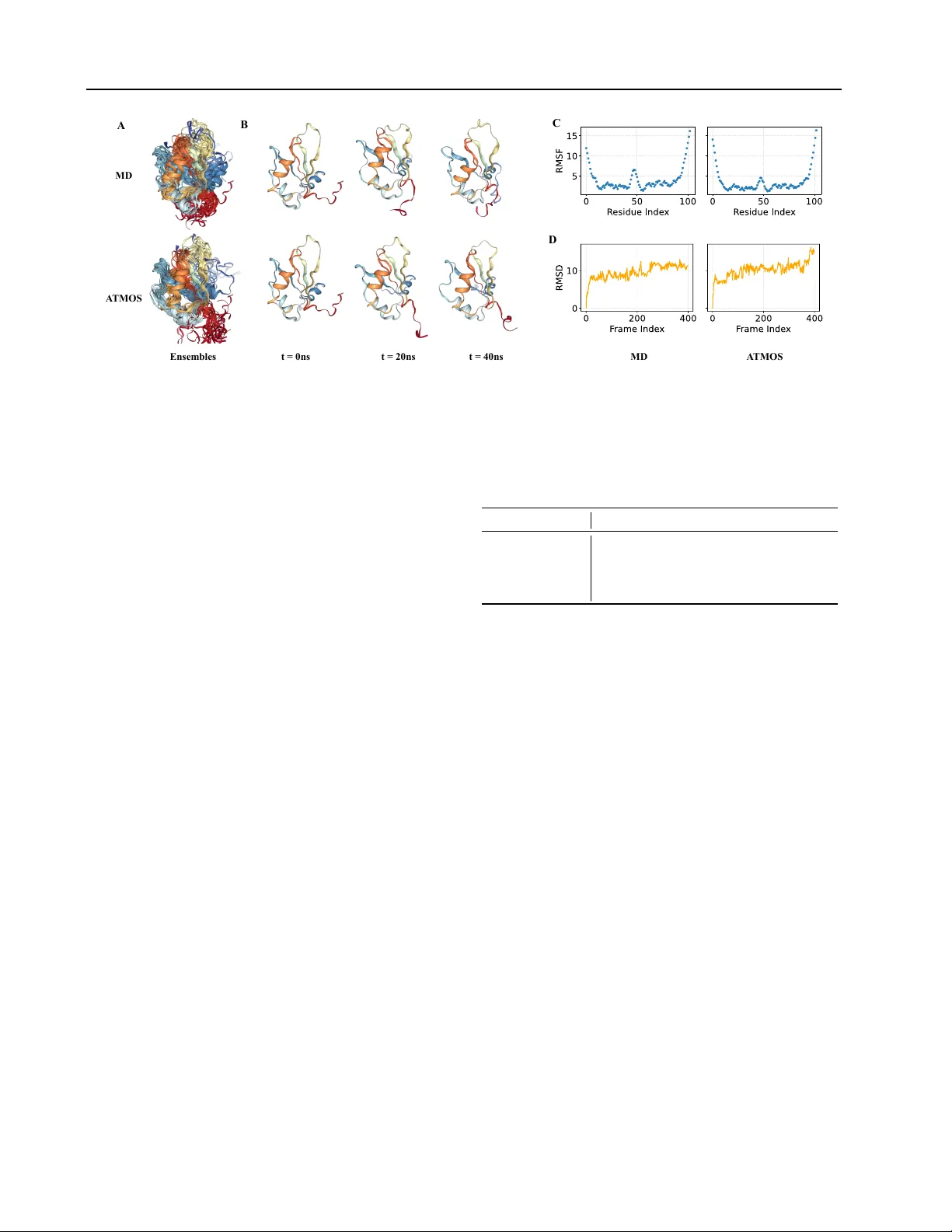
Comments & Academic Discussion
Loading comments...
Leave a Comment