Real-Time Online Learning for Model Predictive Control using a Spatio-Temporal Gaussian Process Approximation

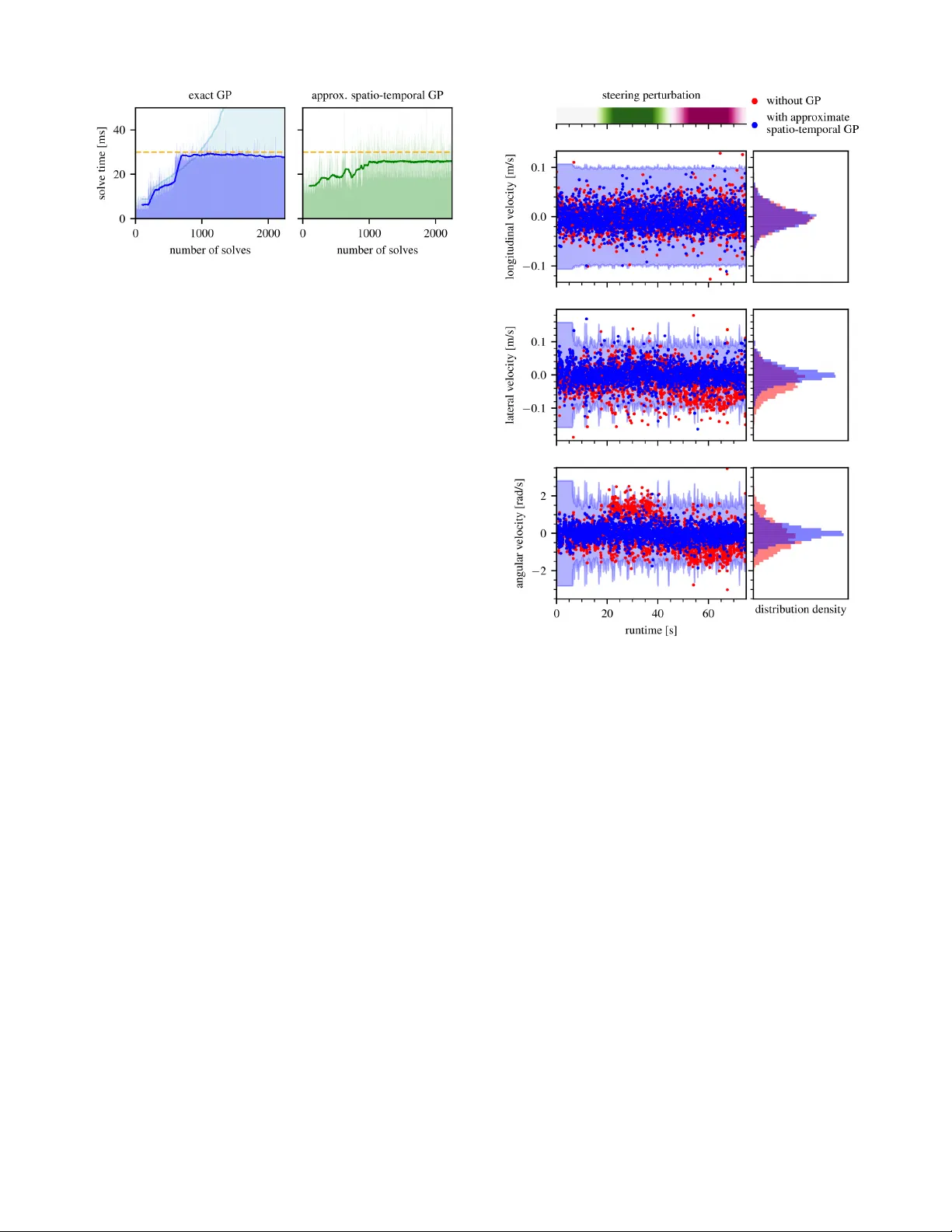
Real-T ime Online Learning f or Model Pr edictiv e Contr ol using a Spatio-T emporal Gaussian Pr ocess A pproximation Lars Bartels, Amon Lahr , Andrea Carron and Melanie N. Zeilinger Abstract — Learning-based model predictive control (MPC) can enhance control perf ormance by corr ecting for model inac- curacies, enabling more precise state trajectory predictions than traditional MPC. A common approach is to model unknown residual dynamics as a Gaussian process (GP), which lev erages data and also provides an estimate of the associated uncertainty . Howev er , the high computational cost of online learning poses a major challenge for real-time GP-MPC applications. This work pres ents an efficient implementation of an approximate spatio-temporal GP model, offering online learning at constant computational complexity . It is optimized for GP-MPC, where it enables improv ed control performance by learning mor e accurate system dynamics online in real-time, even f or time-varying systems. The performance of the proposed method is demonstrated by simulations and hardwar e experiments in the exemplary application of autonomous miniatur e racing . V ideo: https://youtu.be/x4qo66R2- Ds I . I N T R O D U C T I O N Model predictiv e control (MPC) is an advanced control strategy that optimizes control actions by predicting future system behavior based on a dynamic model [1]. By solving an optimization problem at each time step, MPC can handle constraints and adapt to changing conditions, making it highly effecti ve for complex and safety-critical applications. Howe ver , the control performance of traditional MPC relies on the predicti ve capabilities of the underlying model of the system dynamics. For many nonlinear systems, deriving such an accurate model analytically can be impractical. This com- plication motiv ates the incorporation of data-driv en models into the MPC framework [2] to enhance both performance and constraint satisfaction. Gaussian processes (GPs) are a popular choice to model the mismatch between the nominal model and the true sys- tem dynamics in learning-based control, as they offer data- efficient model adaptation and provide formal uncertainty quantification. GP-based MPC (GP-MPC) leverages these properties to maintain high performance and safety under model mismatch and has already been successfully applied across v arious domains (cf. T ab . 2 in [3]), including au- tonomous racing [4], [5]. Ho we ver , the cubic computational scaling of exact GP inference [6] remains a critical bottleneck for real-time GP-MPC. This issue is particularly acute in online learning scenarios, where the continuous accumulation The authors are with the Institute for Dynamic Systems and Control, ETH Z ¨ urich, CH-8092 Z ¨ urich, Switzerland. This work is supported by the European Union’ s Horizon 2020 research and innov ation programme, Marie Skłodowska-Curie grant agreement No. 953348, ELO-X. Fig. 1. High-speed miniature racing despite a time-varying steering perturbation: Online learning using spatio-temporal Gaussian process ap- proximations enables real-time adaptation to time-varying disturbances. The car aims to race along the track centerline (blue) while staying within track boundaries (red) and therefore plans its future trajectory (yellow) including uncertainty estimates based on the GP model of the residual dynamics. of training data ev entually leads to computational latencies that exceed the real-time constraints. A. Appr oximate GP Infer ence for MPC T o maintain real-time feasible computations, [7], [8], [4] use a subset of data (SoD) approximation by conditioning the GP model on a data dictionary containing a fixed number of data points selected from the full training data set. A key challenge with this approach is to decide on which data points to keep in the dictionary based on ho w much rele v ant information they contribute. By replacing old data points in the dictionary with newer ones, [9], [10] allow the GP model to evolve [11], making it suitable for dealing with time-varying disturbances. Inducing-point GP approximations employ a smaller set of strategically placed inducing points to summarize the training data. This reduces computational complexity while preserv- ing essential information for accurate predictions [12], [13], [14]. In the online-learning setting, [8], [4] similarly employ a data dictionary to limit the computational complexity . The finite-dimensional nature of inducing-point GPs also allows for constant-time online updates by updating the inducing- point distribution [15], [16]. Howe ver , for time-varying mod- els, the incurred limited model fidelity necessitates to update also the inducing-point locations to cover the extending input domain. V ariational inducing-point approximations perform this update by re-training on mini-batches of the updated training data set [17], [18], or by performing gradient steps on the “collapsed” evidence lo wer bound [19], [20], which adds to the computation time for online inference. Still, to the best of the authors’ knowledge, these methods hav e seen limited application in the domain of predicti ve control. In this regard, existing GP-MPC applications [21], [4] have resorted to heuristics, dynamically placing inducing points along the previously predicted trajectory , since these locations repre- sent the most rele v ant region in time and space at the current MPC iteration. The dual GP approach proposed by [22] instead employs a time-inv ariant inducing-point GP for long- term learning, complemented by an additional short-term model adapting to variations ov er time online by recursiv ely phasing out old data. Spatio-temporal GPs as described in [23], [24], [25], [26] are naturally well-suited for application in time-v arying settings. They e xploit Markovian temporal cov ariance struc- tures to re write the GP prior as a state-space model defined through a stochastic dif ferential equation [27] according to their kernel, allowing to use Kalman filtering for learning at a constant computational cost per added data point. In the context of MPC, a similar formulation is used by [28]; howe ver , it is limited to purely temporal data. The authors of [29] additionally include a discrete non-temporal oper- ating condition , but they also do not allo w for data in a continuous space as it naturally arises from a dynamic system. T o benefit from the complementary strengths of both inducing-point GPs in space and spatio-temporal GPs in time, the two approaches ha ve been combined by [30], [31] into an approximate spatio-temporal GP model by constructing a Markov chain to track the ev olution of a set of spatial inducing points ov er time. B. Contribution In this work, we dev elop an approximate spatio-temporal GP model based on [31], tailored to the application in a GP- MPC setting. The proposed approach enables ef ficient real- time inference and life-long online learning by recursiv ely adapting to ne w data ov er time at a constant computational cost. Unlik e the recursiv e short-term GP of [22], it supports more intricate temporal covariances, and in contrast to other work on spatio-temporal GP-MPC [28], [29], it allo ws to operate ov er a continuous spatial input space. W e provide an open-source implementation of this model to integrate into the L4acados GP-MPC framework [32], expanding its feature set by a GP model that is particularly suitable to online learning of a time-v arying mismatch in the nominal dynamics. The effecti veness of the proposed method is demonstrated through experiments in the ex emplary real- world application of autonomous miniature racing. I I . P RO B L E M S T A T E M E N T W e consider a system with the general nonlinear discrete- time dynamics x ( k + 1) = f ( x ( k ) , u ( k )) + B g ( x ( k ) , u ( k ) , t k ) + w ( k ) , (1) where x ( k ) ∈ R n x denotes the system state and u ( k ) ∈ R n u is the control input at time t k . The system dynam- ics are composed of the time-in variant nominal dynamics f : R n x × R n u → R n x , the unknown and potentially time- varying residual dynamics g : R n x × R n u × R + → R n g with linear mapping B ∈ R n x × n g , and random process noise w assumed as i.i.d. Gaussian with zero mean and cov ariance Σ w . The residual dynamics are modeled as a Gaussian process such that g ( x, u, t ) ∼ N ( µ g ( x, u, t ) , Σ g ( x, u, t )) , (2) where the mean µ g and co v ariance matrix Σ g can be ev alu- ated at the gi ven v alues for ( x, u, t ) . A. Stochastic OCP F ormulation Follo wing the usual MPC approach, we aim to control the system with dynamics (1) by optimizing state trajectories ov er a receding horizon of length T . Therefore, consider a stochastic OCP of the general form min x,u E " l T ( x T ) + T − 1 X i =0 l i ( x i , u i ) # s.t. x i +1 = f ( x i , u i ) + B g ( x i , u i , t i ) + w i , P ( h j ( x i , u i ) ≤ 0) ≥ p j for j = 1 , . . . , n h x 0 = x ( k ) . (3) Here, the control task is to minimize an expected cost function defined by the sum of stage costs l ( x i , u i ) and a terminal cost l T ( x T ) . At the same time, the system is subject to n h distinct chance constraints, imposing that the indi vidual probability of a constraint h j ( x i , u i ) ≤ 0 being satisfied is at least p j . The interplay of the nonlinear nominal dynamics and the stochastic residual dynamics results in future state distribu- tions whose exact computation is generally intractable [33]. Hence, directly solving the stochastic OCP (3) is challenging without further simplification. B. Deterministic OCP F ormulation In order to obtain a tractable OCP , we approximate the system state distribution as Gaussian, parametrized by its mean µ x and covari ance Σ x as in [5]. Therefore, consider a first-order T aylor approximation around the mean µ x of the uncertainty propagation Σ x k +1 = Ψ( µ x k , Σ x k , u k , t k ) , (4) Ψ( µ x , Σ x , u, t ) = ˜ A Σ x ˜ A ⊤ + B Σ g ( µ x , u, t ) B ⊤ + Σ w , (5) where ˜ A = ∂ ∂ x [ f ( x, u ) + B µ g ( x, u, t )] x = µ x denotes the Jacobian of the nominal and GP mean dynamics. Using the Gaussian approximation of the state distrib ution, the stochastic chance constraints can be reformulated by deterministic tightened constraints with the tightenings gi ven according to the uncertainty in the predictions as h Σ j ( µ x , u, Σ x ) = α j q C j ( µ x , u )Σ x C ⊤ j ( µ x , u ) , (6) where C j ( x, u ) = ∂ ∂ x h j ( x, u ) and the tightening factor is giv en by the inv erse cumulati ve density function of a standard Gaussian distribution as α j = Φ − 1 ( p j ) . In a common approximation to the expected cost [5], we consider only the mean state in the cost function, i.e., E [ l i ( x i , u i )] ≈ l i ( µ x i , u i ) . In combination with the lin- earized cov ariance propagation (5) and constraint tighten- ings (6), this results in a nonlinear OCP whose optimization variables ( µ x , Σ x , u ) are all defined deterministically . C. Zer o-Or der Optimization Although a deterministic OCP can be formulated with the approximations discussed abo ve, actually solving it remains challenging due to the high number of optimization variables and computationally expensi ve GP e valuations. Thus, these approximations alone are often insufficient to enable a real- time capable controller . The zero-order SQP algorithm presented in [34], [35], [36] is an approach to greatly reduce computational cost and still find a feasible, albeit suboptimal, solution to the OCP . This algorithm assumes the cov ariance propagation (5) to ha ve zero gradient with respect to µ x and u during optimization. Follo wing the recent implementations [37], [32], we further neglect the gradients of the constraint tightenings (6). The zero-order approximation thereby allows the elimination of the state covariances Σ x as optimization variables. Instead, Σ x and the resulting v alues of h Σ can be precomputed based on the previous iterate ( ˆ µ x , ˆ u ) of the optimizer . This results in the reduced-size OCP min µ x ,u l T ( µ x T ) + T − 1 X i =0 l i ( µ x i , u i ) s.t. µ x i +1 = f ( µ x i , u i ) + B µ g ( µ x i , u i , t i ) , h j ( µ x i , u i ) + ˆ β ( i ) j ≤ 0 for j = 1 , . . . , n h , µ x 0 = x ( k ) , (7) where ˆ β ( i ) j = h Σ j ( ˆ µ x i , ˆ u i , ˆ Σ x i ) with ˆ Σ x being computed according to (5) based on ( ˆ µ x , ˆ u ) . The algorithm [34] then proposes to solve the OCP (7) iteratively with SQP , where the fixed constraint tightenings ˆ β are updated between SQP iterations. I I I . R E A L - T I M E S P A T I O - T E M P O R A L G P - M P C For enabling a real-time capable GP-MPC strategy with online learning, we combine the zero-order GP-MPC algo- rithm [36] with an approximate spatio-temporal GP model presented by [31]. On this foundation, we contribute an ef fi- cient spatio-temporal GP algorithm by specifically tailoring and optimizing the model for application in an MPC setting. A. Appr oximate Spatio-T emporal GP Model The residual dynamics (2) are modeled as a GP with the spatial input features z =  x ⊤ u ⊤  ⊤ and the temporal input feature t . W e assume this GP to have zero prior mean for sim- plicity and its kernel to be separable as k (( z , t ) , ( z ′ , t ′ )) = k s ( z , z ′ ) k t ( τ ) into a spatial kernel k s and a stationary temporal kernel k t with τ = t − t ′ . This separability allo ws us to treat the spatial and temporal component of the GP independently according to the approach outlined in [31]. The spatial component of the kernel is approximated using a set of inducing points V placed at M fix ed locations in space. Let the inducing-point values v k ∈ R M at any fixed time t k follow a Gaussian distrib ution, whose mean µ ( k ) v and cov ariance Σ ( k ) v may change ov er time. Conditioned on v k , the distrib ution of an observ ation y k at spatial inputs Z k and time t k only depends on the spatial k ernel component k s by the GP conditional y k | v k ∼ N  K Z k V K − 1 V V v k , K Z k Z k − Q Z k Z k + Σ ϵ  , (8) where K ∗∗ is a spatial cov ariance matrix such that [ K AB ] i,j = k s ( A i , B j ) for two sets ( A, B ) of spatial input points. Here, we define Q Z k Z k = K Z k Z k − K Z k V K − 1 V V K V Z k and denote by Σ ϵ the measurement noise variance. In accordance with the standard inducing-point GP inference equations [12], the laws of total expectation and total v ariance yield the distrib ution of the function v alue g ( z , t ) ∼ N ( µ g ( z , t ) , Σ g ( z , t )) with µ g ( z , t ) = K Z V K − 1 V V µ ( t ) v , Σ g ( z , t ) = K Z Z − K Z V K − 1 V V ( K V V − Σ ( t ) v ) K − 1 V V K V Z . (9) In the temporal component, the procedure presented in detail in [25], [27] is applied. This approach uses the Fourier transform of the stationary temporal kernel by (approxi- mately) letting F [ k t ( τ )]( ω ) = W ( iω ) W ( − iω ) such that W ( s ) is a rational transfer function representing a linear time-in variant state-space model with dynamics matrix F , input matrix G , and output matrix H . If k t is a member of the half-integer Mat ´ ern kernels, an explicit formula to compute ( F , G, H ) is given in appendix A. The e volution ov er time of the inducing points is then described by the discrete-time linear Gaussian state-space model ¯ v 0 ∼ N (0 , K V V ⊗ P ∞ ) , ¯ v k +1 | ¯ v k ∼ N (( I M ⊗ A k ) ¯ v k , K V V ⊗ Q k ) , v k = ( I M ⊗ H ) ¯ v k , (10) whose state transition matrices are defined as Kro- necker products (denoted by ⊗ ) of A k = exp(∆ t k F ) and Q k = P ∞ − A k P ∞ A ⊤ k , where ∆ t k = t k +1 − t k , exp( ∗ ) denotes a matrix exponential, and the stationary covariance P ∞ is given as the solution to the continuous-time L yapunov equation F P ∞ + P ∞ F ⊤ = − GG ⊤ . Since the stochastic state-space model (10) and the ob- servation conditional (8) are both fully linear and Gaussian, the standard Kalman filtering technique [38] can be applied to recursiv ely learn the inducing mean µ ( k ) v and cov ari- ance Σ ( k ) v . For simplicity of notation, define ¯ A k = I M ⊗ A k , ¯ Q k = K V V ⊗ Q k , and ¯ C k = K Z k V K − 1 V V ( I M ⊗ H ) . The re- cursiv e estimation scheme first predicts the ne w mean and cov ariance by applying the Markovian state transition model (10) to the pre vious estimate ˆ µ ( k ) ¯ v = ¯ A k − 1 µ ( k − 1) ¯ v , ˆ Σ ( k ) ¯ v = ¯ A k − 1 Σ ( k − 1) ¯ v ¯ A ⊤ k − 1 + ¯ Q k − 1 . (11) Then, the Kalman gain K k = ˆ Σ ( k ) ¯ v ¯ C ⊤ k  ¯ C k ˆ Σ ( k ) ¯ v ¯ C ⊤ k + R k  − 1 , (12) where R k = K Z k Z k − Q Z k Z k + Σ ϵ , allo ws to update the current estimate based on the most recent measurements y k : µ ( k ) ¯ v = ˆ µ ( k ) ¯ v + K k  y k − ¯ C k ˆ µ ( k ) ¯ v  , Σ ( k ) ¯ v =  I M d − K k ¯ C k  ˆ Σ ( k ) ¯ v . (13) B. Spatio-T emporal GP Infer ence for MPC For applicability of the spatio-temporal GP model pre- sented above in an MPC setting, ensuring computational efficienc y is of paramount importance in the algorithm design, as GP-MPC imposes strict real-time constraints on computations for GP learning and inference at each time step. A common and po werful measure to improve efficiency is caching inv ariant and reoccurring expressions preemptiv ely in order to av oid expensi ve repeating computations. For instance, the product K Z V K − 1 V V appears multiple times in the inference equations (9) and does not need to be recomputed. In MPC, it usually holds that the step size ∆ t between consecutiv e time steps is constant. This allows for additional computational savings since the discrete-time state transition matrices A, Q from (10) in the GP model consequently also become in variant and can thus be cached. Also note that by choosing ∆ t = 0 , we can model a time-in v ariant GP . Beyond computational efficienc y , prev ention of numerical instabilities is another critical challenge. Recursiv e algo- rithms can be susceptible to small errors amplifying over time and culminating in inaccurate results. In Kalman filter - ing, such errors can cause the estimated covariance matrix to become indefinite, rendering the estimation algorithm in valid. T o prevent this, the proposed algorithm takes inspi- ration from the square-root Kalman filter [39] and always computes the cov ariance matrix in its Cholesky decompo- sition. While this introduces some additional computational cost, it ensures that the cov ariance matrix remains positi ve semi-definite after each update, preserving the integrity of the Kalman filter . The proposed algorithm of an approximate spatio-temporal GP model comprises three methods, which are presented in Alg. 1, 2, 3 respecti vely . The model is first initialized by computing the state-space representation of the temporal kernel, caching in variant terms, and obtaining the prior inducing-point distribution. Then, the model can be updated to transition to the next time step and incorporate new data if it is av ailable. Finally , the GP can be ev aluated at giv en spatial inputs to provide an uncertainty-aware residual dynamics estimate as required for stochastic MPC. C. Python Implementation & Integr ation into L4acados The proposed implementation is designed for compatibil- ity with GPyTorch [40], le veraging its core functionalities for e v aluating GP kernel functions and Gaussian distrib u- tions. This inte gration allo ws us to rely on the PyTorch [41] automatic differentiation feature for computing the Jacobian of GP predictions required by the optimization algorithm. Algorithm 1 Initialize Approximate Spatio-T emporal GP Require: • GP with zero mean, spatial kernel k s , temporal half- integer Mat ´ ern kernel k t , noise σ 2 ϵ • spatial inducing-point locations V • time step size ∆ t ▷ state-space representation of temporal kernel 1: compute ( F , G, H ) from k t by using (15) 2: obtain P ∞ by solving F P ∞ + P ∞ F ⊤ = − GG ⊤ ▷ cache inv ariant expr essions 3: compute K V V by e valuating k s 4: K 1 / 2 V V = c hol ( K V V ) 5: ¯ H = I M ⊗ H 6: ¯ A = I M ⊗ A with A = exp (∆ t · F ) 7: ¯ Q 1 / 2 = K 1 / 2 V V ⊗ chol ( Q ) with Q = P ∞ − AP ∞ A ⊤ 8: K − 1 / 2 V V = ( K 1 / 2 V V ) − 1 9: L = K − 1 / 2 V V ¯ H ▷ initialize inducing-point distribution 10: µ ¯ v ← 0 M d 11: Σ 1 / 2 ¯ v ← K 1 / 2 V V ⊗ chol ( P ∞ ) Algorithm 2 Update Approximate Spatio-T emporal GP 12: procedure U P DAT E G P( Z ∈ R n z , y ∈ R n y ) 13: µ ¯ v ← ¯ Aµ ¯ v 14: Σ root ¯ v ← h ¯ A Σ 1 / 2 ¯ v ¯ Q 1 / 2 i 15: if ne w data ( Z, y ) is av ailable then 16: compute K Z Z and K Z V by e valuating k s 17: Q root Z Z = K Z V K − 1 / 2 V V 18: R = K Z Z − Q root Z Z ( Q root Z Z ) ⊤ + σ 2 ϵ I | Z | 19: ¯ C = Q root Z Z L 20: P = ¯ C Σ root ¯ v 21: K = ˆ Σ root ¯ v P ⊤  P P ⊤ + R  − 1 ▷ Kalman gain 22: µ ¯ v ← µ ¯ v + K  y − ¯ C µ ¯ v  23: Σ root ¯ v ←  Σ root ¯ v − K P K c hol ( R )  24: end if 25: Σ 1 / 2 ¯ v ← chol  Σ root ¯ v (Σ root ¯ v ) ⊤  26: end procedure Algorithm 3 Evaluate Approximate Spatio-T emporal GP 27: function E V A L U A T E G P ( Z ∈ R N × n z ) 28: compute K Z Z and K Z V by e valuating k s 29: ¯ C = K Z V K 1 / 2 V V L 30: ˆ µ (0) ¯ v = µ ¯ v and ˆ Σ (0) ¯ v = ˆ Σ 1 / 2 ¯ v ( ˆ Σ 1 / 2 ¯ v ) ⊤ 31: for k = 1 , . . . , N do 32: ˆ µ ( k ) ¯ v = ¯ A ˆ µ ( k − 1) ¯ v 33: ˆ Σ ( k ) ¯ v = ¯ A ˆ Σ ( k − 1) ¯ v ¯ A ⊤ + ¯ Q 34: m [ k ] = ¯ C k ˆ µ ( k ) ¯ v ▷ ¯ C k = ¯ C [ k, :] 35: S [ k ] = ¯ C k ˆ Σ ( k ) ¯ v ¯ C ⊤ k 36: end f or 37: µ =  m [1] · · · m [ N ]  ⊤ 38: Σ = K Z Z − Q root Z Z ( Q root Z Z ) ⊤ + diag  S [1] , . . . , S [ N ]  39: retur n N ( µ, Σ) 40: end function Our Python implementation of an approximate spatio- temporal GP model can be accessed as a contribution to L4acados 1 [32], which provides a frame work for learning- based MPC, including an ef ficient GP-MPC implementation utilizing the zero-order SQP optimization algorithm [36]. W ithin L4acados , the proposed model can be used inter- changeably with the existing standard GPyTorch models to capture residual dynamics as a GP . Thereby , we expand the feature set of L4acados by a GP model that enables GP- MPC with online learning at a constant computational cost per time step without neglecting any data. I V . AU T O N O M O U S M I N I A T U R E R AC I N G A. Contr ol T ask T o demonstrate the presented implementation, we apply a GP-MPC controller utilizing the proposed approximate spatio-temporal GP model in autonomous miniature racing simulations and on hardware 2 . The en vironment for these experiments is pro vided by the CRS platform [42]. The car is controlled by a model predicti ve contouring control (MPCC) formulation as it has been presented in [43]. It aims to find the optimal torque a and steering angle δ to maximize progress along the track parametrized by θ while respecting the track boundaries. For our experiments, we use an MPCC controller with a horizon length of T = 40 that is called at a frequenc y of 30Hz . Accordingly , the MPC model dynamics are discretized with a 1 30 s time step size. The nominal car dynamics are adopted from [42] as a dynamic bicycle model with a simplified Pacejka tire friction model [44]. It has a six dimensional state con- taining the car’ s position ( x p , y p ) and orientation φ in the global reference frame as well as the associated ve- locities ( v x , v y , ω ) in the car’ s reference frame. T ogether with the control inputs ( a, δ, θ ) , which are added as an additional integrator state, this results in the system state x =  x p y p φ v x v y ω a δ θ  ⊤ ∈ R 9 and control input u =  u T u δ u θ  ⊤ ∈ R 3 . A time-varying model perturbation is introduced by dy- namically altering the neutral steering of fset δ 0 , as depicted in Fig. 2. This setup serves as a controllable and reproducible proxy for real disturbances, which allows to isolate and ev aluate the controller’ s online learning capability . Note that this perturbation does not physically limit the vehicle’ s ma- neuverability . Since the full range of steering angles remains accessible, the theoretically optimal racing performance is preserved, provided the learning-based controller success- fully identifies and compensates for the mismatch. Each run begins with δ 0 at its nominal value of zero, such that only inherent disturbances are present in the system. After 15s , the value of δ 0 starts to vary with an amplitude of 0 . 15rad . The perturbation directly affects the true dynamics of the linear and angular velocities ( v x , v y , ω ) . Hence, the residual dynamics of these three states are modeled as 1 Code: https://github.com/IntelligentControlSystems/l4acados 2 Experiment data and video material: doi:10.3929/ethz-c-000796944, https://gitlab .ethz.ch/ics/spatio-temporal-gp-mpc Fig. 2. Steering perturbation mapping parametrized by the neutral steering offset δ 0 (red dot). The shaded area illustrates the set of all employed perturbation mappings, with magenta indicating positive v alues and green indicating negati ve values of δ 0 . a GP . The co variance function of this GP is defined as the product of a spatial RBF kernel with input fea- tures ( v x , v y , ω , a, δ ) and a one-time-differentiable temporal Mat ´ ern kernel (exponent ν = 1 . 5 ) with time t as its only input feature. For the learning-based MPCC, we then apply a zero-order GP-MPC strategy [32] with real-time iteration (R TI) [45], where the residual dynamics are modeled by the specified GP . GP hyper-parameters are commonly obtained via minimization of the negati ve marginal log-likelihood or the evidence lower bound [13], determining the parameters that best explain the training data. In our experiments, we hav e additionally found that choosing a “smoother” GP posterior mean and cov ariance improv es con vergence of the optimizer, rendering larger lengthscale hyperparameters desirable. Consequently , we select the GP hyperparame- ters via gradient-based optimization of the marginal log- likelihood, incorporating lo wer bounds on the lengthscale values. Hyperparameter values are the same across all GPs. A controller baseline is provided by a nominal MPCC controller , as used for example in [43], [42], without any awareness on the mismatch between nominal model and real system. Depending on the perturbation, open-loop predic- tions by the MPCC may be highly inaccurate and the car must purely rely on controller feedback to pre vent crashing. Besides the GP-MPC strategy utilizing our approximate spatio-temporal GP model implementation, we also apply an exact GP model with a spatio-temporal kernel and a con ven- tional, purely spatial inducing-point GP model for reference. In order to maintain real-time capable online learning, the latter two rely on a subset-of-data approximation follo wing the GP-MPC example from [32]. Regardless of which model is applied, the inclusion of a GP provides the MPC controller with an estimate on the prediction uncertainty . After the first lap has been completed, online learning is activ ated and the GP model successi vely incorporates newly gathered data points, enabling it to adapt its mean and variance estimates Fig. 3. Experimental GP-MPC solve times using dif ferent GP models with thick lines representing a rolling average of the last 100 solves. Left: Exact GP with a SoD approximation using the 400 most recent data points (blue), compared to simulation results using the full dataset (light blue). Right: Proposed approximate spatio-temporal GP model with 80 spatial inducing points based on hardware experiments (green). of the residual dynamics to the real system. B. Contr oller P erformance Comparison The following results were obtained from real-world rac- ing experiments, conducted as described above. 1) Computational P erformance: Due to the real-time con- straint, we aim for the total GP-MPC computation time to remain below 30ms . W ith the zero-order SQP R TI algorithm, only a single quadratic subproblem of (7) is solved per time step. These computations are relatively fast (belo w 7ms ), which leaves GP learning and inference as the main contributor to the total computational cost. The solve times plotted in Fig. 3 compare GP-MPC using our approximate spatio-temporal GP implementation with standard exact GP-MPC. It is clear that continuously incorporating more data into an exact GP through online learning is not computationally feasible in the long term. For our experiments, we therefore used a SoD approximation, conditioning the GP only on the most recent 400 data points and discarding the rest, which allows to mostly satisfy the computational sub- 30ms constraint. The approximate spatio- temporal GP is not limited through scaling with the amount of data points and it can be observed that solve times remain roughly constant at all times, allo wing to run GP-MPC with online learning indefinitely without neglecting any data. 2) Predictive P erformance: The efficac y of the GP’ s online adaptation may be assessed by the one-step-prediction error between the car’ s actual state and the MPC predicted state from the previous step. The plots in Fig. 4 show this error for the nominal MPC and the proposed spatio-temporal GP-MPC approaches. Depending on the steering perturbation currently present in the system, it can be seen how relying on the nominal model results in a significant model mismatch in the lateral velocity and angular velocity dynamics. Learning this nominal mismatch online with the proposed approxi- mate spatio-temporal GP model implementation considerably reduces the MPC prediction error such that the remaining residual appears independently distributed. While not sho wn in the plot, the exact GP model with spatio-temporal kernel achieves a similar prediction accu- Fig. 4. One-step MPC prediction error over experiment runtime without a GP (red) and with online learning by an approximate spatio-temporal GP (blue) with a 2- σ confidence interval to model the residual dynamics. The bar up top illustrates the time-varying steering perturbation present in the system with the neutral steering offset δ 0 transitioning from zero through positiv e (green) and neg ativ e (magenta) values and back to zero. racy despite the SoD truncation, whereas the purely spatial inducing-point GP produces inconsistent prediction errors since its kernel lacks the temporal dimension necessary to distinguish between varying disturbance states at the same spatial coordinates. 3) Racing P erformance: Ho w the reduction in prediction error affects racing performance in terms of lap times is shown in Fig. 5 for all four controller variants under the same steering perturbation. For the first 15s , there is no steering perturbation present and all controllers result in a similar racing performance. As soon as the perturbation commences, it is obvious that the nominal MPC is unable to maintain this performance lev el. In contrast, with the proposed approximate spatio- temporal GP model adapting to the changing conditions, the controller’ s performance le vel remains largely unaffected by the perturbation. It can also be noted that the SoD exact GP model performs similarly well, indicating that its buf fer of 400 data points is sufficient to carry all temporally Fig. 5. Evolution of the most recent lap times over the experiment runtime under a time-varying steering perturbation for nominal MPC (red squares) and GP-MPC with an e xact GP model (SoD) (orange diamonds), a spatial con ventional inducing-point GP model (SoD) (purple triangles), and an approximate spatio-temporal GP model (blue circles). The exact GP and spatial inducing-point GP employ a subset of data approximation and are conditioned on the most recent 400 data points. Lap times are recorded and plotted at the moment the car has completed a lap. The bar up top illustrates the time-varying steering perturbation present in the system with green corresponding to a positiv e neutral steering offset δ 0 and magenta con versely indicating a negati ve value. relev ant information in this scenario. For the complete data persistence of our approach to offer a significant performance benefit here, the residual dynamics might have to e volv e more slo wly relati ve to the data accumulation rate, causing the buf fer to discard relev ant data points before the system could re visit those spatial locations. More context to the differing racing performance is giv en by the trajectories of the car on track over the full experiment run for nominal MPC and approximate spatio-temporal GP- MPC shown in Fig. 6. It can be observed that the steering calibration perturbation clearly hinders the nominal con- troller to drive the car on a stable racing line. In particular, the car follo ws an undulating trajectory on the straights and the safety margin to the track boundary is violated in some corners. Meanwhile, the GP-MPC controller is able to adapt and compensate for the changing perturbation, which allows the car to maintain much more consistent racing lines throughout the experiment runtime. V . C O N C L U S I O N The proposed spatio-temporal GP-MPC strategy offers a principled and computationally feasible approach to predic- tiv e control with online learning. The underlying approxi- mate spatio-temporal GP model preserves the flexibility and probabilistic rigor of conv entional GPs, but is naturally much better suited to continuous online learning since it can be conditioned on an arbitrary number of data points without negati vely affecting the computational cost of inference. In contrast to other GP-based methods, this enables consistent Fig. 6. Trajectory of racing car on track under a time-varying steering perturbation controlled by nominal MPC without GP (left) and approximate spatio-temporal GP-MPC with online learning (right). real-time capability of closed-loop control without necessi- tating concessions such as discarding parts of the collected data. The resulting potential for performance benefits of the presented real-time implementation has been demonstrated in autonomous miniature racing experiments. For future work, it would be interesting to inv estigate how hyper-parameters can be similarly updated online, and theoretical closed-loop guarantees can be established. A P P E N D I X A. State-Space Representation of Mat ´ ern K ernel For the stationary temporal kernel k t of the spatio- temporal GP , we focus on the family of half-inte ger Mat ´ ern cov ariance functions as they permit an exact state-space representation. The covariance between two points in time separated by τ is then giv en as k t ( τ ) = 2 1 − ν Γ( ν )  √ 2 ν τ σ t  ν K ν  √ 2 ν τ σ t  , (14) where Γ denotes the gamma function, K ν denotes the mod- ified Bessel function of the second kind, σ t is the temporal length scale, and ν = D − 1 / 2 for a positiv e integer D is a smoothness parameter such that the resulting GP is D − 1 times dif ferentiable. In accordance with [27] the state-space system matrices for such a Marko vian kernel can be directly computed as F =      0 1 0 . . . . . . 0 0 1 − a 1 γ D − a 2 γ D − 1 · · · − a D γ      , G =      0 . . . 0 1      , H =  q 0 · · · 0  , (15) where γ = √ 2 ν /σ t , a i =  D i − 1  denote binomial coefficients, and q = (( D − 1)!) 2 (2 D − 2)! (2 γ ) 2 D − 1 defines the dif fusion coefficient. R E F E R E N C E S [1] C. E. Garc ´ ıa, D. M. Prett, and M. Morari, “Model predicti ve control: Theory and practice—A surve y , ” A utomatica , vol. 25, no. 3, 1989. [2] L. He wing, K. P . W abersich, M. Menner , and M. N. Zeilinger , “Learning-Based Model Predicti ve Control: T ow ard Safe Learning in Control, ” Annu. Rev . Control Robot. Auton. Syst. , vol. 3, no. 1, 2020. [3] A. Scampicchio, E. Arcari, A. Lahr, and M. N. Zeilinger , “Gaussian processes for dynamics learning in model predicti ve control, ” 2025. [4] J. Kabzan, L. He wing, A. Liniger , and M. N. Zeilinger , “Learning- Based Model Predicti ve Control for Autonomous Racing, ” IEEE Robot. Autom. Lett. , vol. 4, no. 4, 2019. [5] L. Hewing, J. Kabzan, and M. N. Zeilinger, “Cautious Model Predic- tiv e Control Using Gaussian Process Regression, ” IEEE Tr ansactions on Contr ol Systems T echnology , vol. 28, no. 6, 2020. [6] C. W illiams and C. Rasmussen, “Gaussian Processes for Regression, ” Advances in neural information pr ocessing systems , vol. 8, 1995. [7] D. Nguyen-Tuong and J. Peters, “Incremental online sparsification for model learning in real-time robot control, ” Neur ocomputing , vol. 74, no. 11, 2011. [8] A. Ranganathan, M.-H. Y ang, and J. Ho, “Online Sparse Gaussian Process Regression and Its Applications, ” IEEE T ransactions on Imag e Pr ocessing , vol. 20, no. 2, 2011. [9] M. Maiworm, D. Limon, and R. Findeisen, “Online learning-based model predictiv e control with Gaussian process models and stability guarantees, ” International Journal of Robust and Nonlinear Control , vol. 31, no. 18, 2021. [10] D. Ber gmann, K. Harder, J. Niemeyer , and K. Graichen, “Nonlinear MPC of a Heavy-Duty Diesel Engine W ith Learning Gaussian Process Regression, ” IEEE T rans. Contr . Syst. T echnol. , vol. 30, no. 1, 2022. [11] D. Petelin and J. Kocijan, “Evolving Gaussian process models for predicting chaotic time-series, ” in 2014 IEEE Confer ence on Evolving and Adaptive Intelligent Systems (EAIS) , 2014. [12] J. Quinonero-Candela and C. E. Rasmussen, “ A unifying view of sparse approximate Gaussian process regression, ” The Journal of Machine Learning Resear ch , vol. 6, 2005. [13] M. Titsias, “V ariational Learning of Inducing V ariables in Sparse Gaussian Processes, ” in Pr oceedings of the T welfth International Confer ence on Artificial Intelligence and Statistics , ser . Proceedings of Machine Learning Research, vol. 5. Hilton Clearwater Beach Resort, Clearwater Beach, Florida USA: PMLR, 2009. [14] A. G. d. G. Matthews, J. Hensman, R. T urner , and Z. Ghahramani, “On Sparse V ariational Methods and the Kullback-Leibler Diver gence be- tween Stochastic Processes, ” in Pr oceedings of the 19th International Confer ence on Artificial Intelligence and Statistics , ser . Proceedings of Machine Learning Research, vol. 51. Cadiz, Spain: PMLR, 2016. [15] L. Csat ´ o and M. Opper , “Sparse On-Line Gaussian Processes, ” Neural Computation , vol. 14, no. 3, 2002. [16] H. Bijl, J.-W . van W ingerden, T . B. Sch ¨ on, and M. V erhaegen, “Online sparse Gaussian process regression using FITC and PITC approximations, ” IF AC-P apersOnLine , vol. 48, no. 28, 2015. [17] J. Hensman, N. Fusi, and N. D. Lawrence, “Gaussian Processes for Big Data, ” 2013. [18] C.-A. Cheng and B. Boots, “Incremental variational sparse Gaussian process regression, ” Advances in Neural Information Pr ocessing Sys- tems , vol. 29, 2016. [19] T . D. Bui, C. Nguyen, and R. E. Turner , “Streaming Sparse Gaussian Process Approximations, ” in Advances in Neur al Information Pr ocess- ing Systems , vol. 30. Curran Associates, Inc., 2017. [20] W . J. Maddox, S. Stanton, and A. G. W ilson, “Conditioning Sparse V ariational Gaussian Processes for Online Decision-making, ” in Ad- vances in Neural Information Processing Systems , vol. 34. Curran Associates, Inc., 2021. [21] L. He wing, A. Liniger, and M. N. Zeilinger , “Cautious NMPC with Gaussian Process Dynamics for Autonomous Miniature Race Cars, ” in 2018 European Control Conference (ECC) , 2018. [22] Y . Liu, P . W ang, and R. T ´ oth, “Learning for predictive control: A Dual Gaussian Process approach, ” Automatica , vol. 177, p. 112316, Jul. 2025. [23] J. Hartikainen and S. Sarkka, “Kalman filtering and smoothing solu- tions to temporal Gaussian process regression models, ” in 2010 IEEE International W orkshop on Machine Learning for Signal Processing . Kittila, Finland: IEEE, 2010. [24] S. Sarkka, A. Solin, and J. Hartikainen, “Spatiotemporal Learning via Infinite-Dimensional Bayesian Filtering and Smoothing: A Look at Gaussian Process Re gression Through Kalman Filtering, ” IEEE Signal Pr ocess. Mag. , vol. 30, no. 4, 2013. [25] A. Carron, M. T odescato, R. Carli, L. Schenato, and G. Pillonetto, “Machine learning meets Kalman Filtering, ” in 2016 IEEE 55th Confer ence on Decision and Control (CDC) . Las V egas, NV , USA: IEEE, 2016. [26] M. T odescato, A. Carron, R. Carli, G. Pillonetto, and L. Schenato, “Efficient spatio-temporal Gaussian regression via Kalman filtering, ” Automatica , vol. 118, 2020. [27] S. S ¨ arkk ¨ a and A. Solin, Applied Stochastic Differ ential Equations , 1st ed. Cambridge University Press, 2019. [28] N. Schmid, J. Gruner , H. S. Abbas, and P . Rostalski, “ A real-time GP based MPC for quadcopters with unknown disturbances, ” in 2022 American Contr ol Conference (ACC) , 2022. [29] Y . Li, R. Chen, and Y . Shi, “Spatiotemporal learning-based stochastic MPC with applications in aero-engine control, ” Automatica , vol. 153, 2023. [30] J. Hartikainen, J. Riihim ¨ aki, and S. S ¨ arkk ¨ a, “Sparse Spatio-temporal Gaussian Processes with General Likelihoods, ” in Artificial Neural Networks and Machine Learning – ICANN 2011 . Berlin, Heidelber g: Springer , 2011. [31] W . T ebbutt, A. Solin, and R. E. Turner , “Combining pseudo-point and state space approximations for sum-separable Gaussian Processes, ” in Proceedings of the Thirty-Seventh Conference on Uncertainty in Artificial Intelligence . PMLR, 2021. [32] A. Lahr, J. N ¨ af, K. P . W abersich, J. Frey , P . Siehl, A. Carron, M. Diehl, and M. N. Zeilinger , “L4acados: Learning-based models for acados, applied to Gaussian process-based predictiv e control, ” 2024. [33] A. Girard, C. Rasmussen, J. Q. Candela, and R. Murray-Smith, “Gaus- sian Process Priors with Uncertain Inputs Application to Multiple-Step Ahead T ime Series Forecasting, ” in Advances in Neural Information Pr ocessing Systems , vol. 15. MIT Press, 2002. [34] A. Zanelli, J. Frey , F . Messerer , and M. Diehl, “Zero-Order Rob ust Nonlinear Model Predictive Control with Ellipsoidal Uncertainty Sets, ” IF AC-P apersOnLine , vol. 54, no. 6, 2021. [35] X. Feng, S. D. Cairano, and R. Quirynen, “Inexact Adjoint-based SQP Algorithm for Real-Time Stochastic Nonlinear MPC, ” IF A C- P apersOnLine , vol. 53, no. 2, 2020. [36] A. Lahr, A. Zanelli, A. Carron, and M. N. Zeilinger, “Zero-order optimization for Gaussian process-based model predictive control, ” Eur opean Journal of Contr ol , vol. 74, 2023. [37] J. Frey , Y . Gao, F . Messerer, A. Lahr , M. Zeilinger, and M. Diehl, “Efficient Zero-Order Robust Optimization for Real-Time Model Pre- dictiv e Control with acados, ” 2023. [38] R. E. Kalman, “ A New Approach to Linear Filtering and Prediction Problems, ” Journal of Basic Engineering , vol. 82, no. 1, 1960. [39] P . Kaminski, A. Bryson, and S. Schmidt, “Discrete square root filter- ing: A survey of current techniques, ” IEEE T ransactions on Automatic Contr ol , vol. 16, no. 6, 1971. [40] J. R. Gardner, G. Pleiss, D. Bindel, K. Q. W einberger , and A. G. W il- son, “GPyT orch: Blackbox Matrix-Matrix Gaussian Process Inference with GPU Acceleration, ” 2021. [41] A. Paszke, S. Gross, F . Massa, A. Lerer, J. Bradbury , G. Chanan, T . Killeen, Z. Lin, N. Gimelshein, L. Antiga, A. Desmaison, A. Kopf, E. Y ang, Z. DeV ito, M. Raison, A. T ejani, S. Chilamkurthy , B. Steiner, L. Fang, J. Bai, and S. Chintala, “PyT orch: An Imperative Style, High-Performance Deep Learning Library , ” in Advances in Neural Information Pr ocessing Systems , vol. 32. Curran Associates, Inc., 2019. [42] A. Carron, S. Bodmer , L. V ogel, R. Zurbr ¨ ugg, D. Helm, R. Rick- enbach, S. Muntwiler, J. Sieber, and M. N. Zeilinger, “Chronos and CRS: Design of a miniature car-like robot and a software frame work for single and multi-agent robotics and control, ” in 2023 IEEE International Conference on Robotics and Automation (ICRA) , 2023. [43] A. Liniger, A. Domahidi, and M. Morari, “Optimization-based au- tonomous racing of 1:43 scale RC cars, ” Optimal Contr ol Applications and Methods , vol. 36, no. 5, 2015. [44] R. Rajamani, V ehicle Dynamics and Contr ol . Springer Science & Business Media, 2011. [45] M. Diehl, H. Bock, and J. Schloder, “Real-T ime Iterations for Non- linear Optimal Feedback Control, ” in Proceedings of the 44th IEEE Confer ence on Decision and Contr ol , 2005.