rSDNet: Unified Robust Neural Learning against Label Noise and Adversarial Attacks

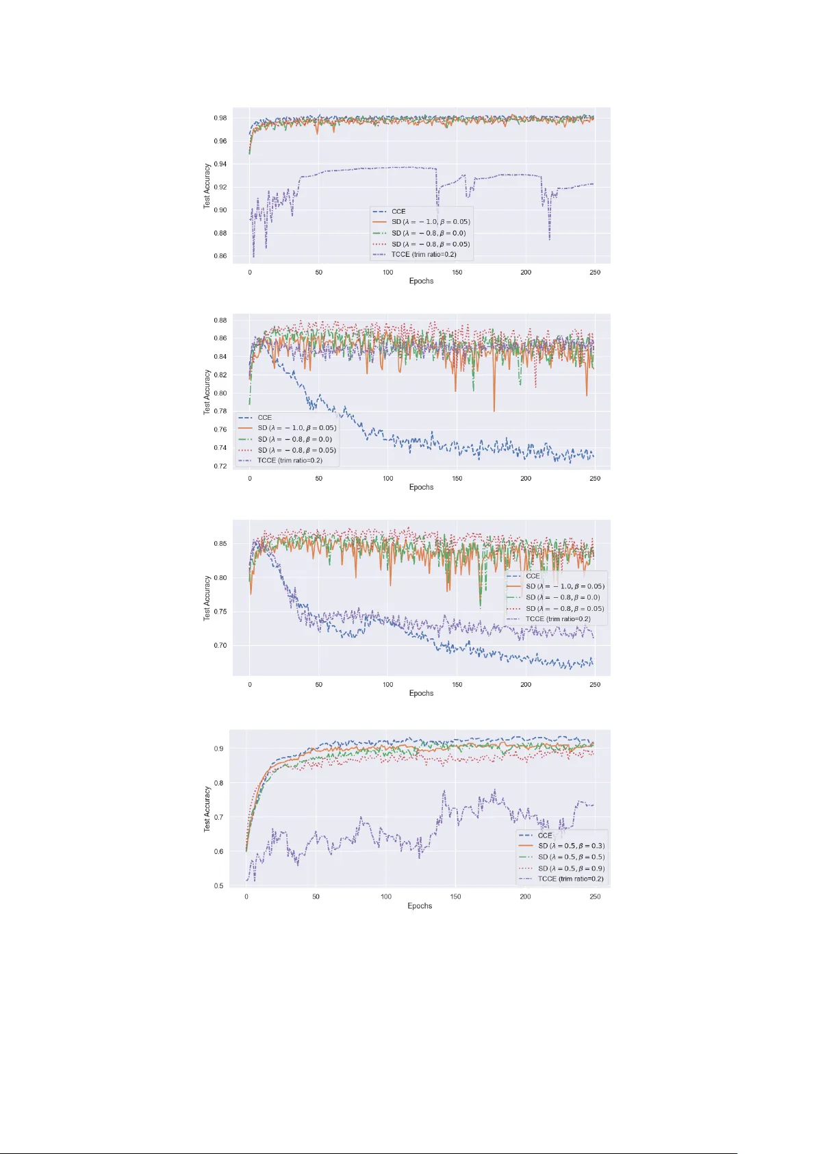
rSDNet: Uniﬁed Robust Neural Learning against Lab el Noise and Adv ersarial A ttac ks Sury asis Jana 1 and Abhik Ghosh ∗ 1 1 Indian Statistical Institute, Kolk ata, India Abstract Neural net works are cen tral to modern artiﬁcial in telligence, y et their training remains highly sensitiv e to data contamination. Standard neural classiﬁers are trained b y minimizing the cate- gorical cross-en tropy loss, corresponding to maxim um lik eliho od estimation under a m ultinomial mo del. While statistically eﬃcien t under ideal conditions, this approach is highly vulnerable to con taminated observ ations including label noises corrupting sup ervision in the output space, and adversarial p erturbations inducing worst-case deviations in the input space. In this pa- p er, we prop ose a uniﬁed and statistically grounded framework for robust neural classiﬁcation that addresses b oth forms of contamination within a single learning ob jective. W e formulate neural net work training as a minim um-divergence estimation problem and in tro duce rSDNet, a robust learning algorithm based on the general class of S -divergences. The resulting training ob jective inherits robustness properties from classical statistical estimation, automatically down- w eighting aberrant observ ations through mo del probabilities. W e establish essen tial p opulation- lev el properties of rSDNet, including Fisher consistency , classiﬁcation calibration implying Bay es optimalit y , and robustness guaran tees under uniform label noise and inﬁnitesimal feature con- tamination. Exp erimen ts on three b enchmark image classiﬁcation datasets show that rSDNet impro ves robustness to lab el corruption and adversarial attacks while maintaining comp etitiv e accuracy on clean data, Our results highlight minim um-divergence learning as a principled and eﬀectiv e framew ork for robust neural classiﬁcation under heterogeneous data contamination. Keyw ords: Neural netw ork classiﬁer; robust learning; S -div ergences; densit y p o wer div ergence; adv ersarial attacks; MLP; CNN. 1 In tro duction Deep neural netw orks form the backbone of modern machine learning and artiﬁcial intelligence (AI) systems, driving adv ances in vision, language, sp eec h, healthcare, and autonomous decision- making. Their success is mainly due to the expressive p o wer and univ ersalit y of neural netw ork (NN) arc hitectures ( Hornik et al. , 1989 ), which facilitate ﬂexible mo deling of complex data structures. T raining is commonly p erformed via empirical risk minimization on large-scale datasets, implicitly assuming that sample observ ations faithfully represent the underlying distribution and are free from con tamination. As neural training is increasingly inﬂuencing high-stakes AI applications across industry and so ciet y , ensuring its robustness has become a foundational requirement for the stability , safet y , and trustw orthiness of mo dern AI systems. In practice, how ever, training data are often contaminated, resulting in signiﬁcantly p oorer p er- formance of neural learning systems. Tw o most prev alent sources of suc h corruption in neural ∗ Corresponding author: abhik.ghosh@isical.ac.in 1 classiﬁcation are lab el noise and adv ersarial p erturbations, aﬀecting output and input spaces, re- sp ectiv ely . Both distort empirical risk compromising the reliabilit y and generalization. Although traditionally studied separately , they b oth may b e viewed as structured forms of distributional con- tamination. This uniﬁed p erspective motiv ates the central question of this work: can robustness to heterogeneous data deviations be achiev ed directly through a suitably deﬁned training ob jectiv e? Addressing this question, we develop a uniﬁed, statistically grounded minim um-divergence learning framew ork for neural classiﬁcation, termed rSDNet, which provides inherent stability against b oth t yp es of contamination within a single ob jective. Learning with noisy lab els has received substantial attention, motiv ated b y annotation errors, w eak sup ervision, crowd-sourced lab eling, and large-scale w eb-based data collection. Neural clas- siﬁers are commonly trained using the categorical cross-entrop y (CCE) loss, whic h corresp onds to the maximum lik eliho o d (ML) estimation under a multinomial mo del ( Go odfellow e t al. , 2016 ). Due to inherent non-robustness of ML estimation, NNs trained with CCE loss tend to memorize mislab eled samples yielding p oor generalization ( Natara jan et al. , 2013 ; Zhang et al. , 2017 ). Ex- isting solutions include loss correction metho ds that explicitly mo del or estimate noise transition mec hanisms ( Patrini et al. , 2017 ), sample selection and reweigh ting strategies ( Han et al. , 2018 ; Ren et al. , 2018 ), and alternative noise-robust loss functions, such as mean absolute error (MAE) and related losses ( Ghosh et al. , 2017b ), generalized cross-entrop y (GCE) of Zhang and Sabuncu ( 2018 ), symmetric cross-entrop y (SCE) based on the symmetric Kullback–Leibler divergence ( W ang et al. , 2019 ), trimmed CCE (TCCE) of Rusiec ki ( 2019 ), and fractional classiﬁcation loss (FCL) of Kurucu et al. ( 2025 ). A comprehensive survey is av ailable in Song et al. ( 2022 ). How ev er, these approaches are primarily tailored to output-space lab el corruption and generally do not address adversarial p erturbations in the input space. Adv ersarial robustness addresses a structurally related vulnerabilit y , namely small, carefully crafted input p erturbations that induce high-conﬁdence misclassiﬁcation while remaining nearly imp erceptible ( Szegedy et al. , 2013 ; Go odfellow et al. , 2014 ). F rom a learning-theoretic p ersp ectiv e, suc h p erturbations represen t worst-case local deviations from the nominal data distribution, thereby constituting contamination in feature space. Adv ersarial training remains the dominant defense strategy , explicitly optimizing mo del parameters against w orst-case p erturbations within a prescrib ed norm ball ( Madry et al. , 2017 ). Ho w ever, this approach typically incurs substantial computational o verhead and may often reduce clean-data accuracy ( Zhang et al. , 2019 ; Rice et al. , 2020 ). Related line of works includes certiﬁed robustness guarantees and distributionally robust optimization under b ounded p erturbations ( Sinha et al. , 2018 ; Cohen et al. , 2019 ; Zhang et al. , 2019 ). In this w ork, instead of attack-speciﬁc defenses, we develop a single principled robust loss that provides resilience across diverse adversarial p erturbation strategies. More broadly , robust NN learning has evolv ed along t wo primary methodological directions. The ﬁrst mo diﬁes net work architectures or training pro cedures to reduce sensitivit y to corrupted obser- v ations. F or example, regularization mech anisms such as drop out ( Sriv asta v a et al. , 2014 ) hav e b een sho wn to improv e robustness against lab el noises in certain settings ( Rusiecki , 2020 ). The second adopts a more fundamental statistical viewpoint, constructing loss functions that down-w eight aber- ran t observ ations, and is closely related to distributionally robust optimization against adversarial attac ks. While these developmen ts highligh t the potential of statistically grounded ob jectives for mitigating contamination eﬀects, most of the formal robust loss theory has b een developed in re- gression con texts ( Rusiecki , 2007 , 2013 ; Ghosh and Jana , 2026 ), while those for classiﬁcation are often tailored to sp eciﬁc corruption mo dels ( Qian et al. , 2022 ). Consequen tly , a common training ob jective that simultaneously addresses b oth output- and input-space con tamination within neural classiﬁcation remains unexplored. In this work, w e formulate neural classiﬁcation as a minimum-div ergence estimation problem and prop ose a uniﬁed robust learning framework, termed rSDNet, based on the general class of S -divergences ( Ghosh et al. , 2017a ). The S -divergence family provides a t wo-parameter formulation con taining b oth the β -divergence ( Basu et al. , 1998 ) and the Cressie–Read pow er div ergence ( Cressie and Read , 1984 ). It has b een formally sho wn to yield highly eﬃ cien t and robust statistical inference under p oten tial data contamination ( Ghosh , 2015 ; Ghosh and Basu , 2017 ). By translating these robustness prop erties to NN classiﬁcation, rSDNet establishes a principled risk minimization strategy 2 in whic h stabilit y arises intrinsically from the curv ature and inﬂuence down-w eighting characteristics of the loss (divergence). Through theoretical analysis and controlled empirical exp eriments under b oth lab el corruption and adv ersarial p erturbations, we demonstrate that robustness can emerge as an inherent prop ert y of the learning ob jectiv e itself, rather than as an auxiliary defense mechanism. The rest of the pap er is organized as follows. The prop osed rSDNet framework is developed in Section 2 along with necessary notations and assumptions. In Section 3 , w e establish key theoret- ical properties of rSDNet, including Fisher consistency and the classiﬁcation calibration prop ert y justifying its Bay es optimalit y . Here we also in vestigate the theoretical robustness guarantees of rS- DNet under b oth uniform lab el noises and inﬁnitesimal contamination. Empirical studies on image classiﬁcation tasks using three widely used benchmark datasets are presented in Section 4 , which further supp ort our theoretical ﬁndings. Finally , some concluding remarks are given in Section 5 . All technical pro ofs, a discussion on the conv ergence rate of the proposed rSDNet algorithm, and detailed results from our numerical exp eriments are deferred to App endices A – C . 2 The prop osed robust learning framew ork 2.1 Mo del setup and notations Consider a J -class classiﬁcation problem with a set of n independent training observ ations S n = { ( y i , x i ) : i = 1 , 2 , . . . , n } , where x i ∈ X ⊆ R p denotes the i -th input feature vector and y i = ( y i 1 , . . . , y iJ ) ⊤ is the one-hot enco ded categorical resp onse vector indicating the class lab el of x i , for i = 1 , . . . , n . Th us, y i ∈ Y = { e 1 , e 2 , . . . , e J } , where e j denotes the j -th canonical basis vector in R J , and y i = e j if and only if x i b elongs to class j , for each i, j . If we denote the random class lab el corresp onding to x i b y Y i ∈ { 1 , 2 , . . . , J } , then we can also write y i = e Y i for each i ≥ 1. Let us assume that the sampled observ ations ( y i , x i ) are indep enden t and identically distributed (I ID) realizations of the underlying random vectors ( Y , X ), and the conditional distribution of the one-hot enco ded resp onse Y , giv en X = x , is Multinomial(1; p ∗ 1 , . . . , p ∗ J ), where p ∗ j ( x ) = P ( Y = e j | X = x ) denotes the p osterior probability of class j = 1 , . . . , J . Throughout we assume that, given any x ∈ X , p ∗ ( x ) = ( p ∗ 1 ( x ) , . . . , p ∗ J ( x )) ⊤ ∈ ∆ ◦ J , the interior of the probability simplex ∆ J =    p = ( p 1 , . . . , p J ) ⊤ ∈ [0 , 1] J : J X j =1 p j = 1    . Our ob jective is to model the relationship b et ween class probabilities and input features to facilitate classiﬁcation of new observ ations. In neural classiﬁcation, we emplo y an NN mo del with J output no des and a softmax activ ation to mo del the p osterior class probabilities p ∗ j ( x ) by p j ( x ; θ ) = e z j ( x ; θ ) P J k =1 e z k ( x ; θ ) , j = 1 , . . . , J, (1) where z j ( x ; θ ) denotes the pre-activ ation (net input) at the j -th output no de, and θ ∈ Θ is the unkno wn mo del parameter consisting of all net work weigh ts and biases. The parameter space Θ dep ends on the assumed NN arc hitecture. This mo del conditional distribution of Y given X is also Multinomial with class probabilities p ( x ; θ ) = ( p 1 ( x ; θ ) , . . . , p J ( x ; θ )) ⊤ , so that the mo del probabilit y mass function (PMF) is given by f θ ( u | x ) = J Y j =1 p u j j ( x ; θ ) , u = ( u 1 , . . . , u J ) ⊤ ∈ Y . (2) If we denote an estimator of θ obtained from the training sample S n b y b θ n , the resulting plug-in classiﬁcation rule (NN classiﬁer) is given b y δ n ( x ) = arg max 1 ≤ j ≤ J p j ( x ; b θ n ). 3 In practice, the parameter v ector θ for an NN classiﬁer is commonly estimated by minimizing the CCE loss function given by L 0 ( θ ) = − 1 n n X i =1 J X j =1 y ij ln p j ( x i ; θ ) , (3) whic h coincides with the ML estimation of the mo del parameters under the multinomial PMF in ( 2 ). Consequently , the resulting classiﬁer inherits the w ell-known sensitivity of ML metho ds to any form of data contamination and mo del missp eciﬁcation. 2.2 Minim um div ergence learning framework The equiv alence b et ween CCE-based training and ML estimation naturally places neural classiﬁ- cation within the broader framework of minimum divergence estimation (MDE). Statistical MDE pro vides a principled approach to parameter estimation, where estimators are obtained by mini- mizing a div ergence b et w een the empirical distribution and a parametric mo del, with the choice of div ergence determining their prop erties. Historically , divergence-based estimation can b e traced bac k to Pearson’s chi-squared div ergence, one of the earliest theoretically grounded approac hes to statistical inference. In recent decades, divergence-based metho ds ha ve received renew ed attention due to their abilit y to pro duce robust estimators with little or no loss in pure data eﬃciency when an appropriate divergence is selected; see, e.g, Basu et al. ( 2011 ). T o formalize this framework in the present setting of NN classiﬁcation (Section 2.1 ), let g ( u | x ), u ∈ Y , denotes the true conditional PMF of Y giv en X = x ∈ X , corresp onding to the Multinomial distribution with true class probabilities p ∗ ( x ), for each i = 1 , . . . , n . Its empirical counterpart at the observed feature v alues is directly obtained as b g i ( u ) := b g ( u | x i ) = I ( u = y i ) for u ∈ Y and i = 1 , . . . , n , where I ( · ) denotes the indicator function. Without assuming any mo del distribution for X , here we are basically mo delling each conditional PMF g i = g ( ·| x i ) by the parametric PMF f i, θ = f θ ( ·| x i ), as given in ( 2 ), o ver observ ed feature v alues x i , i = 1 , . . . , n . Thus, a general minim um divergence estimator b θ n of θ , with resp ect to a statistical divergence measure d ( · , · ), is deﬁned as b θ n = arg min θ 1 n P n i =1 d  b g i , f i, θ  . In particular, the ML estimation corresp onds to the MDE based on the Kullbac k–Leibler diver- gence (KLD) d KL ( · , · ). A straigh tforward calculation yields d KL ( b g i , f i, θ ) = X u ∈Y b g i ( u ) log b g i ( u ) f i, θ ( u ) = − J X j =1 y ij log p j ( x i ; θ ) , since b g i ( e j ) = y ij for all i, j ≥ 1, and hence P u b g i ( u ) log b g i ( u ) = P j y ij log y ij = 0 under one-hot enco ding (with the conv ention 0 · log 0 = 0). Consequen tly , the CCE loss in ( 3 ) can b e expressed as the av erage KLD measure 1 n P n i =1 d KL ( b g i , f i, θ ), Hence, minimizing the CCE loss is exactly equiv alent to minimizing the av erage KLD b et ween the empirical and mo del conditional PMFs. This characterization motiv ates a general minimum divergence learning framework for neural classiﬁers, where the KLD may b e replaced by a suitably chosen alternative divergence to achiev e desirable statistical prop erties. In particular, divergences p ossessing suitable robustness prop erties can substan tially mitigate the sensitivity of ML-based training to con tamination and mo del missp ec- iﬁcation. Here we adopt the particular class of S -div ergences ( Ghosh et al. , 2017a ) to construct our prop osed rSDNet, yielding enhanced robustness under b oth input- and output-space contamination while retaining high statistical eﬃciency under clean data. 2.3 S -Divergence family and the rSDNet ob jectiv e As introduced by Ghosh et al. ( 2017a ), the S -div ergence (SD) b et ween tw o PMFs, g and f having common supp ort Y is deﬁned, dep ending on tw o tuning parameters β ≥ 0 and λ ∈ R , as S β ,λ ( g , f ) = 1 A X u ∈Y f 1+ β ( u ) − 1 + β AB X u ∈Y f B ( u ) g A ( u ) + 1 B X u ∈Y g 1+ β ( u ) , 4 where A = 1+ λ (1 − β )  = 0, and B = β − λ (1 − β )  = 0. When either A = 0 or B = 0, the corresponding SD measures are deﬁned through resp ectiv e contin uous limits. The tuning parameters ( β , λ ) con trol the robustness–eﬃciency trade-oﬀ of the resulting MDE and asso ciated inference. P articularly , β adjusts the inﬂuence of outlying observ ations, so that larger β increases robustness but reduces eﬃciency; v alues of β > 1 are t ypically av oided due to severe eﬃciency loss. On the other hand, λ in terp olates b et ween div ergence families allo wing further (higher-order) con trol o ver robustness while preserving the same ﬁrst-order asymptotic eﬃciency at a ﬁxed β . Ho wev er, Ghosh et al. ( 2017a ) demonstrated that the minimum SD estimators (MSDEs) exhibit go o d robustness only when A ≥ 0. Recen tly , Ro y et al. ( 2026 ) established the asymptotic breakdown p oin t of the MSDEs and asso ciated functionals, conﬁrming high-robustness when A ≥ 0 and B ≥ 0. Both studies further suggest that the b est robustness–eﬃciency trade-oﬀs are obtained for appropriate SD measures with A > 0 and B > 0. Thus, excluding the b oundary cases A = 0 or B = 0, here we restrict ourselves to the SDs with admissible tuning parameters satisfying A > 0 and B > 0, namely T =  ( β , λ ) : − 1 1 − β < λ < β 1 − β , 0 ≤ β < 1  ∪  (1 , λ ) : λ ∈ R  . Note that the second part of T corresp onds to a single div ergence, since the SD reduces to the squared L 2 distance at β = 1, irresp ectiv e of λ . Despite this restriction, T retains most imp ortan t sub classes of the SD family . The choice λ = 0 pro duces β -div ergences or density p ow er divergences (DPDs) of Basu et al. ( 1998 ), while β = 0 giv es the p o wer div ergence (PD) family ( Cressie and Read , 1984 ) with − 1 < λ < 0, including the Hellinger disparity at λ = − 0 . 5. Ho wev er, the set T exclude the non-robust KLD at ( β , λ ) = (0 , 0) and the rev erse KLD (rKLD) at ( β , λ ) = (0 , − 1), the latter kno wn to cause computational diﬃculties in discrete mo dels with inliers ( Basu et al. , 2011 ). More broadly , the SD family can b e view ed as a reparameterization of ( α, β )-divergences ( Cic ho c ki et al. , 2011 ) and also as a sp ecial case of extended Bregman divergences of Basak and Basu ( 2022 ). Under our setup of neural classiﬁcation giv en in Section 2.1 , and following the general discussions in Section 2.2 , we deﬁne the MSDE of the NN mo del parameter θ as b θ ( β ,λ ) n = arg min θ ∈ Θ L ( n ) β ,λ ( θ ) , with L ( n ) β ,λ ( θ ) = 1 n n X i =1 S β ,λ ( b g i , f i, θ ) . (4) W e refer to the resulting neural classiﬁer trained via an MSDE b θ ( β ,λ ) n as rSDNet( β , λ ) for any giv en c hoice of ( β , λ ) ∈ T , and the asso ciated ob jectiv e function L ( n ) β ,λ ( θ ) as rSDNet loss ( empiric al SD- risk ) or rSDNet tr aining obje ctive . W e next study this loss function further to develop a scalable practical implementation of rSDNet. 2.4 The ﬁnal rSDNet learning algorithm F or practical implemen tation of rSDNet, the asso ciated NN training ob jective L ( n ) β ,λ ( θ ) can be ex- pressed in a muc h simpliﬁed form. Substituting the explicit forms of b g i and f i, θ in to the SD expression ( 2.3 ), we obtain the ﬁnal rSDNet training ob jective (loss) as giv en by L ( n ) β ,λ ( θ ) = 1 n n X i =1 ℓ β ,λ ( y i , p ( x i ; θ )) , ( β , λ ) ∈ T , (5) where ℓ β ,λ ( u , p ) = 1 A J X j =1  p 1+ β j − 1 + β B u j p B j + A B  , for ( β , λ ) ∈ T , u ∈ Y , p ∈ ∆ J . (6) Although we restrict ourselves to tuning parameter v alues in T , the rSDNet loss L β ,λ ( θ ) can also b e extended to the b oundary cases of A = 0 or B = 0 by the resp ectiv e con tinuous limits of the form giv en in ( 5 )–( 6 ). W e av oided these b oundary cases as they are exp ected to ha ve practical issues with either outliers or inliers ( Ghosh et al. , 2017a ). 5 Since the rSDNet ob jective L β ,λ ( θ ) in ( 5 ) can b e non-conv ex in θ by the choice of the netw ork arc hitecture in p ( x ; θ ), following standard NN learning pro cedures, we prop ose to solve this opti- mization problem eﬃciently using the Adam algorithm ( Kingma and Ba , 2014 ). It is a ﬁrst-order sto c hastic gradien t metho d, which starts with initializing t wo momen t vectors m 0 and v 0 to the n ull v ector, and up date the minimizer of L β ,λ ( θ ) at the t -th step of iteration by θ t ← θ t − 1 − α c m t /  p b v t + ϵ  , t = 1 , 2 , . . . , (7) where c m t and b v t are, resp ectively , the up dated bias-corrected estimates of ﬁrst and second raw momen ts, given b y c m t ← β 1 m t − 1 + (1 − β 1 ) g t 1 − β t 1 , b v t ← β 2 v t − 1 + (1 − β 2 ) g 2 t 1 − β t 2 , with g t = ∇ θ L β ,λ ( θ t − 1 ) denoting the gradien t of the loss function with resp ect to θ , and g 2 t b eing the vector of squared elemen ts of g t for each t ∈ N . Given the form of the rSDNet loss function in ( 5 )–( 6 ), we can compute its gradient as given by ∇ θ L β ,λ ( θ ) = 1 + β nA n X i =1 J X j =1 h p β j ( x i ; θ ) − y ij p B − 1 j ( x i ; θ ) i ∇ θ p j ( x i ; θ ) , ( β , λ ) ∈ T . (8) F or NN arc hitectures inv olving non-smo oth activ ation functions (e.g., ReLU), its output p j ( x i ; θ ) migh t not b e diﬀeren tiable ev erywhere with respect to θ . In suc h cases, w e need to replace ∇ θ p j ( · ; θ ) in gradient computation by a measurable selection from its sub diﬀeren tial ∂ θ p j ( · , θ ), which is as- sumed to exist for most commonly used NN architectures. F or eﬃcien t implementation of the Adam algorithm, we ha ve used the TensorFlow library ( Abadi et al. , 2016 ) of Python,; it computes the required gradient g t via automatic diﬀerentiation ( Bolte and Pau wels , 2021 ), cov ering the cases of non-smo oth activ ation as well. As initial weigh ts θ 0 in the training pro cess, w e hav e used either of the standard built-in initializers ‘Glorot’ and ‘He’, whic h corresp ond to the normal and uniform base distributions, resp ectiv ely . Throughout our empirical exp erimen tation, we hav e used the default Adam hyperparameter v alues suggested by Kingma and Ba ( 2014 ), which are α = 10 − 3 , β 1 = 0 . 9, β 2 = 0 . 999, and ϵ = 10 − 8 . Python co des for the complete rSDNet training are av ailable through the GitHub rep ository Robust-NN-learning 1 . F ollowing the theory of Adam ( Kingma and Ba , 2014 ), one should ideally contin ue the iterativ e up dation step ( 7 ) un til the sequence { θ t } conv erges. How ev er, in most practical problems, achieving suc h full con vergence is often computationally exp ensiv e. So, Adam up dates are t ypically executed for a predeﬁned n umber of ep o c hs, whic h is generally chosen by monitoring the stability of the test accuracy for the trained classiﬁer. In all illustration presented in this pap er, we employ ed the Adam algorithm for 250 ep ochs, which w as observed to b e suﬃcien t for stable training of rSDNet; see App endix B for an empirical study justifying it for b oth pure and contaminated data. 3 Theoretical guaran tees 3.1 Statistical consistency of rSDNet functionals W e start by establishing that the prop osed rSDNet classiﬁer indeed deﬁnes a v alid statistical classi- ﬁcation rule at the p opulation level, which is essen tial for justifying its use in learning from random training samples under ideal conditions. In this resp ect, we need to deﬁne the p opulation-level func- tionals asso ciated with rSDNet, which characterizes the target parameters that empirical learning pro cedures aim to estimate. W e may note that the MSDE b θ ( β ,λ ) n of the NN mo del parameter θ under rSDNet( β , λ ) may b e re-expressed from ( 4 ) as a minimizer of E G X ,n [ S β ,λ ( b g ( ·| X ) , f θ ( ·| X ))] with resp ect to θ ∈ Θ, 1 https://github.com/Suryasis124/Robust- NN- learning.git 6 where G X ,n denotes the empirical distribution function of X placing mass 1 /n at each observed x i , and b g is the empirical estimate of g based on the training sample S n . Accordingly , w e deﬁne the p opulation-lev el minimum SD functional (MSDF) of θ for tuning parameters ( β , λ ) ∈ T at the true distributions ( G X , g ) as T β ,λ ( G X , g ) = arg min θ ∈ Θ R β ,λ ( θ | G X , g ) with R β ,λ ( θ | G X , g ) = E G X [ S β ,λ ( g ( ·| X ) , f θ ( ·| X ))] , (9) where G X denotes the true distribution function of X and R β ,λ ( θ ) = R β ,λ ( θ | G X , g ) is the p op- ulation SD-risk . At the empirical level, this corresp onds to R β ,λ ( θ | G X ,n , b g ) = L ( n ) β ,λ ( θ ), so that T β ,λ ( G X ,n , b g ) = b θ ( β ,λ ) n . W e refer to the resulting neural classiﬁer obtained by setting θ = T β ,λ ( G X , g ) as the rSDNet functional . The following theorem then presents its Fisher consistency; the pro of is straigh tforward from the fact that SD is a genuine statistical divergence ( Ghosh et al. , 2017a ). Theorem 3.1 (Fisher Consistency of rSDNet) . F or any ( β , λ ) ∈ T , the p osterior class pr ob abilities of the rSDNet functional, obtaine d using the MSDF in ( 9 ) , satisfy p ( x ; T β ,λ ( G X , g )) = p ( x ; θ 0 ) = p ∗ ( x ) a.s. , for any mar ginal distribution G X , pr ovide d that the c onditional mo del is c orr e ctly sp e ciﬁe d with g ≡ f θ 0 for some θ 0 ∈ Θ . The ab ov e theorem shows Fisher consistency and uniqueness of the rSDNet functional at the lev el of class probabilities. A similar result for the MSDF T β ,λ ( G X , g ) requires the following standard iden tiﬁability condition for the assumed NN architecture. (A0) The NN classiﬁer output function x 7→ p ( x ; θ ) is measurable for all θ ∈ Θ, and the parame- terization θ 7→ p ( x ; θ ) is identiﬁable in θ up to known netw ork symmetries, i.e., p ( x ; θ 1 ) = p ( x ; θ 2 ) a.s. ⇒ θ 1 = ð · θ 2 , for some ð in a known symmetry group G acting on the (non-empty) parameter space Θ. Under Assumption (A0) , the MSDF at an y ( β , λ ) ∈ T satisﬁes T β ,λ ( G X , g ) = ð · θ 0 for some ð ∈ G as in (A0) . Thus, T β ,λ ( G X , g ) is unique only up to known NN symmetries, whic h is consistent with standard NN learning theory (see, e.g., Go odfellow et al. , 2016 ; Ghosh and Jana , 2026 ). Bey ond Fisher consistency , the rSDNet functional is also classiﬁc ation-c alibr ate d , meaning that minimization of the p opulation SD-risk R β ,λ ( θ ) yields Bay es-optimal classiﬁcation decisions at the p opulation level ( Zhang , 2004 ; Bartlett et al. , 2006 ; T ewari and Bartlett , 2007 ). T o verify this, let us further simplify the p opulation SD-risk, using the form of SD giv en in ( 2.3 ), as R β ,λ ( θ ) = E G X [ r β ,λ ( p ∗ ( X ) , p ( X ; θ ))] , where we deﬁne the conditional SD-risk r β ,λ ( p ∗ , p ) = 1 A J X j =1  p 1+ β j − 1 + β B p B j p ∗ j A + A B p ∗ j 1+ β  , for ( β , λ ) ∈ T , p , p ∗ ∈ ∆ J . (10) Note that r β ,λ ( u , p ) = ℓ β ,λ ( u , p ) for any u ∈ Y and p ∈ ∆ J , although they diﬀer for an y p ∗ ∈ ∆ ◦ J unless ( β , λ ) = (0 , − 1). F urther, since ( 10 ) corresponds to the SD b et ween p ∗ and p , it is alwa ys non-negativ e and equals zero if and only if p = p ∗ . Consequently , the p opulation SD-risk R β ,λ ( θ ) has a unique minimizer at p = p ∗ for any ( β , λ ) ∈ T . In other words, the SD-loss underlying rSDNet is classiﬁcation-calibrated in the sense of Bartlett et al. ( 2006 ). Hence, the class predicted b y the rSDNet functional coincides with that of the asymptotically optimal Bay es classiﬁer, δ B ( x ) = arg max 1 ≤ j ≤ J p ∗ j ( x ), whic h minimizes the conditional misclassiﬁcation risk. These prop erties of rSDNet are summarized in the following theorem. Theorem 3.2 (Classiﬁcation calibration of rSDNet) . The rSDNet functional at any ( β , λ ) ∈ T is classiﬁc ation-c alibr ate d, and henc e the induc e d classiﬁer achieves the Bayes-optimal class pr e diction at the p opulation level. 7 3.2 T olerance against uniform lab el noise W e now establish the robustness of rSDNet against uniform lab el noise, a widely used output noise mo del in classiﬁcation. Each training lab el is assumed to b e indep enden tly corrupted with proba- bilit y η ∈ [0 , 1]; when corruption occurs, the label is replaced uniformly at random b y one of the remaining class lab els. F ormally , w e represent con taminated training data as S η = { ( e y i , x i ) : i = 1 , 2 , . . . , n } , where the observed lab el e y i = y i with probability 1 − η and equals any incorrect class lab el with probabilit y η / ( J − 1) when the input feature v alue is x i , i ≥ 1. If w e denote the random v ariable corresp onding to e y i b y e Y , then the true conditional distribution of e Y , giv en X = x , is again Multinomial but with PMF g η ( ·| x ) in volving class probabilities p ∗ η ( x ) = ( p ∗ η , 1 ( x ) , . . . , p ∗ η ,J ( x )), where p ∗ η ,j ( x ) = (1 − η ) p ∗ j ( x ) + η J − 1 (1 − p ∗ j ( x )) , j = 1 , . . . , J. W e study the eﬀect of such noise on the exp e cte d SD-loss underlying our rSDNet, given by R β ,λ ( θ ) = E ( Y , X ) h L ( n ) β ,λ ( θ ) i = E ( Y , X ) [ ℓ β ,λ ( Y , p ( X ; θ ))] = E G X [ E g [ ℓ β ,λ ( Y , p ( X ; θ )) | X ]] . Let θ ∗ β ,λ denotes its global minimizer at ( β , λ ) ∈ T . W e compare the minim um achiev able exp ected SD-loss R β ,λ ( θ ∗ β ,λ ) under clean data with that obtained under uniform lab el noise. T o this end, we deﬁne θ η β ,λ to b e the global minimizer of the exp ected SD-risk under uniform lab el noise, given by R η β ,λ ( θ ) = E ( e Y , X ) h L ( n ) β ,λ ( θ ) i = E G X  E g η [ ℓ β ,λ ( Y , p ( X ; θ )) | X ]  . Then w e assess the robustness of rSDNet through the excess risk, R β ,λ ( θ η β ,λ ) − R β ,λ ( θ ∗ β ,λ ). Smaller this diﬀerence close to zero, greater the tolerance of rSDNet against uniform lab el noises. T o derive a b ound for it, we ﬁrst show the uniform b oundedness of the total SD-loss in the following lemma; its pro of is given in App endix A.1 . Lemma 3.3. F or any x ∈ X , θ ∈ Θ , and ( β , λ ) ∈ T , we have J 1 − β A − 1 + β AB max(1 , J 1 − B ) + J 2 B ≤ J X j =1 ℓ β ,λ ( e j , p ( x ; θ )) ≤ J A − 1 + β AB min(1 , J 1 − B ) + J 2 B . (11) Since the total SD-loss in Lemma 3.3 depends on ( x , θ ), it is not symmetric in the sense of Ghosh et al. ( 2017b ). Symmetry arises only at ( β , λ ) = (0 , − 1), corresp onding to the rKLD having A = 0, whic h lies outside our admissible parameter range T ; see W ang et al. ( 2019 ) for neural classiﬁers dev elop ed based on the rKLD and its practical limitations. Although SD-loss is not symmetric and th us not exactly noise-toleran t, rSDNet still exhibits b ounded excess risk under uniform lab el noise for all ( β , λ ) ∈ T . The exact b ound is provided in the following theorem; see App endix A.2 for its pro of. Theorem 3.4. Under uniform lab el noise with c ontamination pr op ortion 0 ≤ η < 1 − 1 /J , the exc ess risk of rSDNet satisﬁes 0 ≤ R β ,λ ( θ η β ,λ ) − R β ,λ ( θ ∗ β ,λ ) ≤ M ( η ) β ,λ , ( β , λ ) ∈ T , (12) wher e M ( η ) β ,λ = η ( J − 1 − J η ) 1 A  J − J 1 − β + 1 + β B | 1 − J 1 − B |  . Note that the b ound M ( η ) β ,λ in Theorem 3.4 decomp oses into t wo comp onen ts: one dep ending on the noise level η and the other on the tuning paramete rs ( β , λ ). The η -dependent factor coincides with that obtained in robust learning literature (e.g., Ghosh et al. , 2017b ), implying the same rate of degradation with increasing noise. In particular, the b ound v anishes as η ↓ 0 and diverges as η ↑ ( J − 1) /J . The second component in M ( η ) β ,λ quan tiﬁes the eﬀect of ( β , λ ) and explains 8 the impro ved robustness of certain rSDNet mem b ers. F or ﬁxed ( η , J ), the b ound decreases as β increases, indicating greater tolerance to uniform lab el noise (see Figure 1 ). The role of λ b ecomes more pronounced at higher contamination levels; for any ﬁxed β ∈ [0 , 1], the b ound is minimized when λ ∈ [ − 1 , 0] and increases rapidly as λ mov es outside this range. (a) η = 0 . 2 (b) η = 0 . 4 (c) η = 0 . 6 Figure 1: Plots of the b ound M η β ,λ on the excess risk of rSDNet, as a function of tuning parameters ( β , λ ), for diﬀerent contamination prop ortion η and J = 10. 3.3 Lo cal robustness against con taminated features W e next ev aluate the lo cal robustness of rSDNet to inﬁnitesimal contamination in the feature space using inﬂuence function (IF) analysis. Since sample-based IFs are often diﬃcult to interpret in deep learning settings (see, e.g., Basu et al. , 2021 ; Bae et al. , 2022 ), we adopt the p opulation-lev el form ulation of IF as originally introduced b y Hampel et al. ( 1986 ). Sp eciﬁcally , w e study the IF of the MSDF T β ,λ ( G X , g ) underlying our rSDNet, under a gross-error contaminated feature distribution G X ,ϵ = (1 − ϵ ) G X + ϵ ∧ x t , where ϵ > 0 denotes the contamination prop ortion at an outlying p oin t x t ∈ X and ∧ x denotes the degenerate distribution at x ∈ X . The IF of T β ,λ at the contamination p oin t x t is formally deﬁned as I F ( x t , T β ,λ , ( G X , g )) = lim ϵ ↓ 0 T β ,λ ( G X , g ) − T β ,λ ( G X ,ϵ , g ) ϵ = ∂ ∂ ϵ T β ,λ ( G X ,ϵ , g )     ϵ =0 , whic h quantiﬁes the eﬀect of inﬁnitesimal contamination at x t on the resulting estimator and hence on the rSDNet framework. In order to derive the expression of this IF at any ( β , λ ) ∈ T , we deﬁne ψ β ,λ ( x ; θ ) = A 1 + β ∇ θ [ r β ,λ ( p ∗ ( x ) , p ( x ; θ ))] = J X j =1 u j ( x ; θ ) ∇ θ p j ( x ; θ ) , (13) with u j ( x ; θ ) = p β j ( x ; θ ) − p ∗ j A ( x ) p B − 1 j ( x ; θ ) , and Ψ β ,λ ( θ ) = A 1 + β ∇ 2 θ R β ,λ ( θ ) = E G X [ ∇ θ ψ β ,λ ( X ; θ )] , = E G X   J X j =1 u ′ j ( X ; θ ) ∇ θ p j ( X ; θ ) ∇ ⊤ θ p j ( X ; θ ) + J X j =1 u j ( X ; θ ) ∇ 2 θ p j ( X ; θ )   , (14) with u ′ j ( x ; θ ) = β p β − 1 j ( x ; θ ) − p ∗ j A ( x )( B − 1) p B − 2 j ( x ; θ ) . As noted earlier, for non-diﬀerentiable NN architectures, ∇ θ in the ab o ve deﬁnitions should b e in terpreted as a measurable elemen t of the corresp onding sub-diﬀerential with resp ect to θ . Then, the following theorem presents the ﬁnal IF for the MSDF; see App endix A.2 for its pro of. 9 Theorem 3.5. F or rSDNet with tuning p ar ameter ( β , λ ) ∈ T , the inﬂuenc e function of the under- lying MSDF T β ,λ under fe atur e c ontamination at x t ∈ X is given by I F ( x t , T β ,λ , ( G X , g )) = − Ψ + β ,λ ( θ g ) ψ β ,λ ( x t , θ g ) + ν ( θ g ) , (15) wher e θ g = T β ,λ ( G X , g ) , ν ( θ g ) ∈ K er ( Ψ β ,λ ( θ g )) , the kernel (nul l-sp ac e) of Ψ β ,λ ( θ g ) , and Ψ + β ,λ r epr esents Mo or e–Penr ose inverse of Ψ β ,λ . R emark 3.1 . F or thin shallo w or under-parameterized NN architectures, the matrix Ψ β ,λ ( θ g ) is t ypically non-singular, and so its Mo ore-P enrose inv erse reduces to the ordinary inv erse. Then, ( 15 ) pro vides the unique IF of the MSDF with ν ( θ g ) = 0 . In more general deep or o ver-parameterized net works, how ever, Ψ β ,λ ( θ g ) is often singular, implying non-uniqueness of the IF. Nevertheless, the dep endence on the con tamination p oin t x t is go verned by the same function ψ β ,λ ( x t ; θ g ) in all cases. Hence, the robustness prop erties of rSDNet under input noise are determined solely by the b eha vior of ψ β ,λ with resp ect to x t . No w, to study the nature of ψ β ,λ ( x t , θ g ), recall that the (mo del) class probabilities arise from an NN with softmax output lay er as sp eciﬁed in ( 1 ). Its (sub-)gradient has the form ∇ θ p j ( x ; θ ) = p j ( x ; θ ) " ∇ θ z j ( x t ; θ ) − J X k =1 p j ( x ; θ ) ∇ θ z k ( x t ; θ ) # , j = 1 , . . . , J. Because 0 ≤ p j , p ∗ j ≤ 1, the weigh ts u j ( x ; θ ) in ( 13 ) are b ounded for all j ≥ 1. Consequently , the b oundedness of ψ β ,λ ( x t ; θ g ), and hence that of the IF, dep ends primarily on the growth of the net work (sub-)gradients ∇ θ p j ( x t ; θ ), which may b e unbounded dep ending on the architecture. The IF remains b ounded ov er an unbounded feature space if either p ( · ; θ g ) ≡ p ∗ , or ∇ θ p j ( x t ; θ ) is b ounded in x t . The ﬁrst condition corresp onds to a correctly sp eciﬁed conditional mo del, in whic h case the IF b ecomes iden tically zero, although this scenario rarely holds in practice even with highly expressiv e NNs. Th us, lo cal robustness of rSDNet under feature contamination is ensured when the netw ork gradients with resp ect to parameters remain controlled. F or any giv en architecture, the parameters β > 0 and λ < 0 further mitigate the growth of ψ β ,λ through the down-w eighting functions u j ( x ; θ ), j = 1 , . . . , J . Increasing β and decreasing λ strengthen this atten uation, thereby impro ving tolerance to mo derate feature contamination. Suc h eﬀects are further clariﬁed though the following simple example. Example 3.1. Consider the binary classiﬁcation problem with a single input feature x ∼ N (0 , 1), X = R , and true p osterior class probability p ∗ ( x ) = ( p ∗ 1 ( x ) , 1 − p ∗ 1 ( x )), where p ∗ 1 ( x ) = e κ ( x ) 1 + e κ ( x ) , κ ( x ) = sin ( x ) + e x + x 5 / 3 . W e mo del it using neural classiﬁers ( 1 ) with J = 2, p 2 ( x, θ ) = 1 − p 1 ( x, θ ), and z 1 ( x, θ ) in the deﬁnition of p 1 ( x, θ ) b eing sp eciﬁed by three NN architectures as follows: (M1) Single la yer p erceptron: z 1 ( x ; θ ) = θ 1 + θ 2 x , with θ = ( θ 1 , θ 2 ) ⊤ . (M2) ReLU hidden lay er: z 1 ( x ; θ ) = θ 5 + θ 6 φ ( θ 1 + θ 2 x ) + θ 7 φ ( θ 3 + θ 4 x ), with φ ( s ) = max(0 , s ) and θ = ( θ 1 , θ 2 , . . . , θ 7 ) ⊤ . (M3) tanh hidden lay er: z 1 ( x ; θ ) = θ 5 + θ 6 tanh( θ 1 + θ 2 x )+ θ 7 tanh( θ 3 + θ 4 x ), with θ = ( θ 1 , θ 2 , . . . , θ 7 ) ⊤ . It is straigh tforward to verify that the (sub-)gradient of z 1 ( x ; θ ) is b ounded in x ∈ R only for (M3), while it grows linearly in x for b oth (M1) and (M2). T o examine lo cal robustness of rSDNet across the three architectures, we numerically ev aluate the IFs of the MSDF for θ at θ g = (1 , . . . , 1) T . The exp ectations E G X , app earing in the expression of IF (Theorem 3.5 ) are approximated by the empirical av erage based on a random sample of size n = 100 drawn from N (0 , 1). The resulting IFs are plotted in Figures 2 – 4 . F or brevity , under (M2) and (M3), we present the IFs only for θ 1 , θ 2 , θ 5 and θ 6 , since the remaining parameters exhibit 10 similar b eha vior. It is evident from the ﬁgures that, for suitably c hosen tuning parameters ( β , λ ), the IFs remain w ell-controlled, often b ounded, with resp ect to the contamination p oin t x t , thereby indicating the lo cal robustness of the corresp onding rSDNet. (a) IFs for θ 1 (b) IFs for θ 2 Figure 2: IFs for the MSDFs of parameters under the NN mo del (M1) in Example 3.1 , for diﬀeren t tuning parameters ( β , λ ). (a) IFs for θ 1 (b) IFs for θ 2 (c) IFs for θ 5 (d) IFs for θ 6 Figure 3: IFs for the MSDFs of parameters under the NN mo del (M2) in Example 3.1 , for diﬀeren t tuning parameters ( β , λ ). 11 (a) IFs for θ 1 (b) IFs for θ 2 (c) IFs for θ 5 (d) IFs for θ 6 Figure 4: IFs for the MSDFs of parameters under the NN mo del (M3) in Example 3.1 , for diﬀeren t tuning parameters ( β , λ ). 4 Empirical Ev aluation on Image Classiﬁcation 4.1 Exp erimen tal setups: Datasets and NN arc hitectures T o assess the ﬁnite-sample p erformance of the prop osed rSDNet, we conducted exp eriments on the follo wing three b enc hmark image classiﬁcation datasets, which were selected b ecause of their widespread adoption in the NN literature and v arying levels of classiﬁcation diﬃculty . • MNIST dataset: It consists of 70000 grayscale images of handwritten digits (0–9), eac h with a spatial resolution of 28 × 28 pixels. Considering each pixel intensit y as an input feature, w e ha ve 784 cov ariates p er image, which were linearly normalized, from their original range [0, 255] to the interv al [0 , 1], prior to mo del training. T o build a neural classiﬁer for this dataset, we emplo yed a fully connected multila yer per- ceptron (MLP) consisting of tw o hidden lay ers with 128 neurons each and ReLU activ ation functions. The output lay er contained 10 neurons with a softmax activ ation function to mo del the categorical class lab els 0–9. • F ashion-MNIST dataset: It also contains 70000 gra yscale images of size 28 × 28 pixels, categorized into 10 clothing classes (e.g., T-shirt/top, trouser, sandal, coat, etc.). As in the MNIST dataset, each image corresp onds to 784 input features represen ting pixel intensities, rescaled to [0, 1] b efore training the NN mo del. The NN arc hitecture w as taken to be a fully connected MLP with tw o hidden la yers con taining 200 and 100 neurons, resp ectiv ely , b oth using ReLU activ ation functions, and 10 softmax neurons in the output lay er. 12 • CIF AR-10 dataset: It consists of 60000 colored (RGB) images represen ting 10 ob ject cate- gories. Each image has a resolution of 32 × 32 pixels with three color channels, yielding 32 × 32 × 3 = 3072 input features, whic h were normalized to [0, 1] as b efore. Giv en the increased complexit y , here we adopted a conv olutional NN (CNN) architecture, consisting of tw o con volutional la yers with 32 and 64 ﬁlters (kernel size 3 × 3, ReLU activ ation), eac h follo wed b y 2 × 2 max-p ooling lay ers. The conv olutional feature maps were ﬂattened and passed through a fully connected lay er with 512 ReLU units, follow ed by a 10-unit softmax output lay er as follo ws: 32 × 32 × 3 (input image) → Conv2D(32 , 3 × 3 , ReLU) → MaxP o ol(2 × 2) → Con v2D(64 , 3 × 3 , ReLU) → MaxPool(2 × 2) → Flatten → Dense(512 , ReLU) → Dense(10 , Softmax) (Output) Generic Mo del T raining and Ev aluation Pro cedure: Although all three datasets provide default training–test splits, av ailable in the TensorFlow library of Python, w e combined the original training and test partitions, and randomly generated k > 1 folds to ev aluate the p erformance of the trained neural classiﬁers using k -fold cross v alidation. F or eac h dataset, we applied the prop osed rSDNet with v arious tuning parameter com binations (and 250 ep ochs), and compared the results with existing b enc hmark loss functions/classiﬁers suc h as CCE, MAE, TCCE( δ ), rKLD, SCE( α, β ), GCE( q ), and FCL( µ ). Here δ denotes the trimming prop ortion, and ( α, β ), q and µ are tuning parameters deﬁning the resp ectiv e loss functions. In all cases, mo del training w as p erformed on b oth clean and suitably contaminated versions of the training folds. Final p erformance of eac h classiﬁer was ev aluated using av erage k -fold cross-v alidated classiﬁcation accuracy computed on uncontaminated test/v alidation folds. The num b er of folds w as set to k = 7 for MNIST and F ashion-MNIST, and k = 6 for CIF AR-10 to match their original training-test split ratio. 4.2 P erformances under clean data The av erage cross-v alidated (CV) classiﬁcation accuracies of all NN mo dels trained on the non- con taminated (clean) datasets are rep orted in T able 1 , for the prop osed rSDNet and existing b enc h- mark learning algorithms. In such cases of clean data, the standard CCE loss ac hiev es strong p erformance across all three datasets, with resp ective accuracy of 0.9816, 0.8891, and 0.6782. The SCE loss and GCE with q = 0 . 5 show comparable results, particularly on MNIST and F ashion- MNIST datasets. Our rSDNet consistently matches, and in sev eral conﬁgurations slightly improv es up on, the CCE baseline. F or MNIST, multiple rSDNet parameter combinations achiev e accuracies sligh tly ab o ve 0.980, with the b est p erformance of 0.9809 attained at ( β , λ ) = (0 . 3 , 0), whic h is essen tially identical to CCE. On F ashion-MNIST, rSDNet reaches a maximum accuracy of 0.8948 at ( β , λ ) = (0 . 1 , − 0 . 5), sligh tly outperforming CCE (0.8891) and SCE (0.8911). F or CIF AR-10, the b est rSDNet accuracy is 0.6729 at ( β , λ ) = (0 . 1 , 0), which is again very comp etitiv e with CCE (0.6782) and SCE (0.6785) losses. Overall, rSDNet maintains comp etitive p erformance across a broad range of ( β , λ ) choices, demonstrating no signiﬁcan t loss in eﬃciency under clean conditions. In contrast, several existing robust alternativ es exhibit clear degradation in accuracy when no con tamination is present. TCCE sho ws progressively worse p erformance as the trimming propor- tion increases, whic h is expected as trimming remov es informativ e observ ations in the absence of outliers. The MAE loss also p erforms adequately on MNIST (0.9770) but substantially underp er- forms on F ashion-MNIST (0.7940) and completely fails on CIF AR-10 (0.1004) datasets, indicating its optimization instability in complex scenarios. A similar phenomenon app ears for FCL at certain parameter settings. In particular, F CL with µ = 0 collapses to near-random performance (accu- racy 0.1) on CIF AR-10, and larger v alues µ ≥ 0 . 5 lead to near-random accuracy on b oth MNIST and F ashion-MNIST. GCE with q = 0 . 7 also shows noticeable deterioration on CIF AR-10 (0.5590), although it remains comp etitiv e on MNIST. These results sho ws extremely high eﬃciency of the prop osed rSDNet compared to its existing robust comp etitors when trained on clean data. Imp ortan tly , this stability holds across a wide range 13 of tuning parameter v alues, suggesting that rSDNet (unlik e other robust learning algorithms) do es not incur a p erformance p enalt y in the absence of contamination. 4.3 Robustness against uniform lab el noises In order to illustrate the p erformances under lab el corruption, uniform lab el noise was introduced b y randomly replacing the true class lab el of a sp eciﬁed prop ortion ( η ) of training observ ations with one of the remaining class lab els. Models were trained on such contaminated training folds, while p erformances w ere ev aluated on clean test folds as b efore. The resulting a verage cross-v alidated accuracies for contamination lev el η = 0.1 to 0.5 are presented in T ables 2 – 4 , respectively , for the three datasets. F or all datasets, the CCE loss sho ws a steady and substantial p erformance degradation as noise increases. Similar deterioration is observed also for SCE and F CL with small µ ≤ 0 . 25. MAE and GCE( q = 0 . 7) remain highly stable for MNIST data, maintaining accuracy ab o ve 0.95 ev en at η = 0 . 5. MAE also shows mo derate robustness for F ashion-MNIST data but ﬂuctuates and falls b elo w stronger comp etitors at higher con tamination levels; it how ever collapses to near-random p er- formance ( ≈ 0.10) across all contamination levels for the more complex CIF AR-10 dataset. Among existing robust losses, GCE p erforms well for F ashion-MNIST data, maintaining relatively high ac- curacy (0.8339) even at η = 0 . 5 for q = 0 . 7, while TCCE(0.2) ac hieves the highest accuracy for CIF AR-10 data at lo w contamination. In con trast, the prop osed rSDNet consistently exhibits strong robustness for all three datasets for small β > 0 (0.05–0.1) and λ < 0 (b et ween − 0 . 5 and − 1). While some existing losses pro vide robustness under sp eciﬁc settings (e.g., MAE on MNIST, or GCE with q = 0 . 7 for F ashion-MNIST), their p erformance is often dataset-dep enden t or unstable for more complex data (e.g., CIF AR-10). The prop osed rSDNet, ho wev er, provides consistently comp etitiv e or sup erior performance across datasets and contamination levels without collapsing ev en under high lab el noise. 4.4 Stabilit y against diverse adv ersarial attacks T o further assess the robustness of the prop osed rSDNet, w e conducted the same empirical ex- p erimen ts under four widely studied white-b o x adv ersarial attacks, namely the fast gradient sign metho d (FGSM) ( Go odfellow et al. , 2014 ), pro jected gradient descent (PGD) ( Madry et al. , 2017 ), Carlini–W agner (CW) attack ( Carlini and W agner , 2017 ), and DeepF o ol attac k ( Mo osa vi-Dezfo oli et al. , 2016 ). Adversarial examples were generated from the MNIST dataset using a surrogate NN mo del, havin g a single hidden lay er of 64 ReLU no des and 10 softmax output no des, trained with the CCE loss for 250 ep o c hs. Separate training folds were constructed using fully adversarial im- ages from each attack with suitable hyperparameter v alues 2 . The same NN mo dels, as b efore, were trained based on these training datasets. In addition to the clean test accuracy , here we also com- puted av erage accuracies on adversarially p erturbed test folds under the same attack. The results are rep orted in T able 5 . Under suc h adv ersarial training, CCE ac hieves high adversarial test accuracy (0.9776 – 0.9949 for F GSM/PGD, and 0.9815 under CW), but its clean test accuracy can drop substan tially , particularly under PGD (0.6516). TCCE sho ws systematic degradation in clean accuracy as the trimming prop ortion increases, with sharp er decline under stronger attac ks. F or example, under PGD training, clean accuracy falls b elow 0.47 for trimming lev els ≥ 0 . 1, indicating that excessiv e trimming remo ves substan tial useful information ev en in structured adversarial settings. In con trast, rSDNet maintains comp etitiv e or sup erior performance across a wide range of tuning parameters. Under FGSM training, it achiev es the highest clean test accuracy (0.9235 at (0 . 9 , 0 . 5)), exceeding CCE, while main taining comparable adversarial accuracy ( ≈ 0 . 975). Under PGD, rSDNet attains the b est adversarial accuracy (0.9958 at (0 . 3 , − 1)) and slightly improv es clean accuracy o ver CCE in certain conﬁgurations (maximum 0.6582 at (1 , 0)). F or CW and DeepF o ol attacks, 2 FGSM with perturbation magnitude 0.3; PGD with attack step size 0.01 and maximum perturbation bound 0.3; untargeted CW with learning rate 0.01; DeepF o ol with ov ershoot parameter 0.02. Maxim um 100 iterations are used in last three cases. 14 rSDNet p erforms similarly to the CCE, with adv ersarial accuracies consistently b et ween 0.978 and 0.985 and clean accuracies close to the b est obse rv ed v alues. The highest DeepF o ol adversarial accuracy (0.9854) is ac hieved at b y rSDNet(0 . 5 , 0 . 5). Generally , rSDNet with mo derate-to-large β > 0 combined with λ ∈ [ − 1 , 0 . 5] yields strong adversarial robustness without sacriﬁcing clean p erformance. No rSDNet conﬁguration exhibits a severe decline in p erformance, and the results remain tightly concentrated across parameter choices. All these v alidate that rSDNet preserves predictiv e accuracy under adversarial training while providing stable and comp etitiv e robustness across div erse attack mechanisms, often matching or exceeding the CCE baseline and av oiding the degradation observed for heavily trimmed losses. 4.5 On the c hoice of rSDNet tuning parameters Based on theoretical considerations and empirical evidence, it is evident that the practical p erfor- mance of rSDNet dep ends heavily on the choice of its tuning parameters ( β , λ ). The pattern is consisten t with prior applications of S -divergences in robust statistical inference; see, e.g., Ghosh et al. ( 2017a ); Ghosh ( 2015 ); Roy et al. ( 2026 ). In the present con text of neural learning as well, rSDNet ac hieves optimal performance under uncon taminated data when β and | λ | are small, whereas larger v alues of β > 0 and λ < 0 are required to obtain stable results in the presence of increasing data contamination. Since the extent of p otential contamination is unknown in most cases, we rec- ommend selecting β ∈ (0 , 0 . 1] and λ ∈ [ − 1 , − 0 . 5], which pro vides a fa vorable robustness-eﬃciency trade-oﬀ across all scenarios considered in our empirical studies. In practice, an optimal pair ( β , λ ) for a giv en datasets ma y be determined via cross-v alidation o ver a grid of feasible v alues within these ranges. 5 Concluding remarks In this work, we utilized a broad and well-kno wn family of statistical divergences, namely the SD family , to construct a ﬂexible class of loss functions for robust NN learning in classiﬁcation tasks. The resulting framework, rSDNet, provides a principled, statistically consistent, Bay es optimal clas- siﬁer, whose robustness and eﬃciency can b e explicitly controlled via its divergence parameters. W e theoretically characterized the eﬀect of these tuning parameters on the robustness of rSDNet and empirically demonstrated its improv ed stability across b enc hmark image-classiﬁcation datasets. With appropriately c hosen parameters, rSDNet preserves predictive accuracy on clean data while oﬀering enhanced resistance to label noise and adversarial perturbations. These results highlight the practical viability of divergence-based training as a robust alternative to conv entional cross-entrop y learning based on p ossibly noisy training data. Nev ertheless, to clearly isolate and understand the eﬀects of divergence-based losses relative to existing metho ds, w e delib erately restricted our exp erimen ts to relatively simple NN arc hitectures, fo cusing primarily on image classiﬁcation. A systematic theoretical and empirical in vestigation of rSDNet in mo dern large-scale deep learning pip elines, incorp orating complex arc hitectures such as residual netw orks, transformer-based mo dels and hybrid attention-based architectures, remains an imp ortan t direction for future work. While w e pro vided initial theoretical insights for rSDNet, a comprehensive analysis of its conv ergence dynamics, generalization guaran tees, and adversarial robustness in deep, non-conv ex, and p oten tially non-smooth net work architectures is y et to b e dev elop ed. F urthermore, broadening the application of rSDNet to other data mo dalities, suc h as text, tabular, graph-structured, and m ultimo dal data, would signiﬁcantly enhance its practical impact, enabling robust learning from large, noisy datasets across diverse scientiﬁc and industrial domains. Most imp ortan tly , w e hop e that the theoretical insights and empirical ﬁndings presented here will motiv ate further research on statistically grounded loss functions and contribute to the developmen t of reliable, robust, and trustw orthy AI systems. 15 A Pro of of the results A.1 Pro of of Lemma 3.3 F rom ( 6 ), we get J X j =1 ℓ β ,λ ( e j , p ( x ; θ )) = J A J X j =1 p 1+ β j − 1 + β AB J X j =1 p B j + J 2 B . (16) W e use the follo wing b ounds for sums of p ow ers of a probabilit y vector p = ( p 1 , . . . , p J ) ∈ ∆ J : • If 0 < r < 1, then P J j =1 p r j ∈ [1 , J 1 − r ]. • If r ≥ 1, then P J j =1 p r j ∈ [ J 1 − r , 1]. No w, since ( β , λ ) ∈ T , using these results, we get J X j =1 p 1+ β j ∈ [ J − ( β ) , 1] , J X j =1 p B j ∈ [min(1 , J 1 − B ) , max(1 , J 1 − B )] . Substituting these b ounds into ( 16 ) we get the desired result giv en in ( 11 ). A.2 Pro of of Theorem 3.4 W e may note that the ﬁrst inequality of ( 12 ) follows directly from the deﬁnition of θ ∗ β ,λ . Next, to prov e the second inequality , we study the excess risk under lab el contamination as R η β ,λ ( θ ) = E G X  E g η [ ℓ β ,λ ( Y , p ( X ; θ )) | X ]  , = (1 − η ) R β ,λ ( θ ) + η J − 1   E G X   J X j =1 ℓ β ,λ ( e j , p ( X ; θ ))   − R β ,λ ( θ )   =  1 − J η J − 1  R β ,λ ( θ ) + η J − 1 T β ,λ ( θ ) , where T β ,λ ( θ ) = E G X h P J j =1 ℓ β ,λ ( e j , p ( X ; θ )) i . But, since θ η β ,λ minimizes R η β ,λ ( θ ), we get R η β ,λ ( θ η β ,λ ) ≤ R η β ,λ ( θ ∗ β ,λ ) , and hence  1 − J η J − 1  R β ,λ ( θ η β ,λ ) + η J − 1 T β ,λ ( θ η β ,λ ) ≤  1 − J η J − 1  R β ,λ ( θ ∗ β ,λ ) + η J − 1 T β ,λ ( θ ∗ β ,λ ) . Rearranging the ab o ve, we get R β ,λ ( θ η β ,λ ) − R β ,λ ( θ ∗ β ,λ ) ≤ η J − 1 − J η h T β ,λ ( θ ∗ β ,λ ) − T β ,λ ( θ η β ,λ ) i . (17) No w, from Lemma 3.3 , the total SD-loss T β ,λ ( θ ) is b ounded for all x , θ , and thus we get T β ,λ ( θ ∗ β ,λ ) − T β ,λ ( θ η β ,λ ) ≤ max θ T β ,λ ( θ ) − min θ T β ,λ ( θ ) = 1 A  J − J 1 − β + 1 + β B | 1 − J 1 − B |  . Substituting it in ( 17 ), we get the desired b ound on the excess loss as given in ( 12 ). 16 A.3 Pro of of Theorem 3.5 F rom the deﬁnition of the statistical functional T β ,λ giv en in ( 9 ), w e can re-express θ g = T β ,λ ( G X , g ) as a solution to the estimating equation E G X [ ψ β ,λ ( X , θ g )] = 0 . (18) Accordingly , θ ϵ = T β ,λ ( G X ,ϵ , g ) satisﬁes the corresp onding estimating equation giv en by E G X ,ϵ [ ψ β ,λ ( X , θ ϵ )] = 0 , whic h can b e expanded to the form: (1 − ϵ ) E G X [ ψ β ,λ ( X , θ ϵ )] + ϵ ψ β ,λ ( x t , θ ϵ ) = 0 . (19) No w, diﬀerentiating b oth side of ( 19 ) with resp ect to ϵ , and ev aluating at ϵ = 0 using ( 18 ), we get E G X [ ∇ θ ψ β ,λ ( X , θ g )] I F ( x t , T β ,λ , ( G X , g )) = ψ β ,λ ( x t , θ g ) . The expression ( 15 ) of the IF is then obtained by solving the ab o ve equation via standard theory of linear equations. B Con v ergence of rSDNet: An empirical study Here w e provide a brief look at the conv ergence b ehavior of the prop osed rSDNet with resp ect to the n umbers of training ep ochs, as this directly determines the computational cost of applying robust rSDNet in practice. F or this purp ose, we reﬁtted the same NN mo dels describ ed in Section 4 on the MNIST and F ashion-MNIST datasets, but now using their default training-test split as provided in TensorFlow . W e then ev aluate test accuracy for mo dels trained ov er a range of epo c hs from 1 to 250. F or both datasets, experiments were rep eated for clean training data and con taminated training data with 20% and 40% uniform label noise. Additionally , for the MNIST dataset, w e also considered adv ersarially p erturb ed training data generated using FGSM attacks. The resulting test accuracies are reported in Figures 5 – 6 for rSDNet with a few representativ e v alues of ( β , λ ) ∈ T , alongside b enc hmark results obtained using the standard CCE loss and its trimmed v ariant TCCE(0.2). The results show that, under clean data, rSDNet exhibits a conv ergence rate comparable to b oth CCE and TCCE(0.2), with all metho ds conv erging within a small num b er of ep ochs. How ever, in the presence of uniform lab el noise, CCE and TCCE displa y slo wer and less stable conv ergence, whereas rSDNet maintains a fast and stable con vergence b ehavior similar to that observ ed in the clean-data scenario. Under adversarial corruption as well, rSDNet ac hieves con vergence speeds com- parable to CCE, while TCCE-based metho ds conv erge signiﬁcantly more slowly . These ﬁndings demonstrate that rSDNet can b e eﬀectively applied to practical datasets, whether clean or contam- inated by structured noise, without incurring additional computational cost to achiev e desired level of robustness. 17 (a) Clean training data (b) Contaminated training data with 20% uniform lab el noise (c) Contaminated training data with 40% uniform lab el noise (d) Contaminated training data under FGSM adv ersarial attack Figure 5: T est accuracies obtained b y diﬀerent NN learning metho ds trained with v arying n umbers of ep ochs for the MNIST dataset 18 (a) Clean training data (b) Contaminated training data with 20% uniform lab el noise (c) Contaminated training data with 40% uniform lab el noise Figure 6: T est accuracies obtained b y diﬀerent NN learning metho ds trained with v arying n umbers of ep ochs for the F ashion-MNIST dataset 19 C T ables con taining empirical results T able 1: Av erage k -fold CV accuracies of the NN classiﬁers trained on the three selected datasets using the proposed rSDNet with diﬀeren t ( β , λ ) and the b enc hmark losses/classiﬁers under clean data [ k = 7 for MNIST and F ashion-MNIST, and k = 6 for CIF AR-10] Dataset → MNIST F ashion-MNIST CIF AR-10 Existing losses for neural classiﬁcation CCE 0.9816 0.8891 0.6782 MAE 0.9770 0.7940 0.1004 TCCE(0.1) 0.9354 0.8815 0.6733 TCCE(0.2) 0.8665 0.3094 0.6687 TCCE(0.3) 0.7787 0.2939 0.6275 rKLD 0.9643 0.8803 0.6240 SCE( α = 0 . 5 , β = 1) 0.9809 0.8911 0.6785 GCE( q = 0 . 5) 0.9788 0.8932 0.6629 GCE( q = 0 . 7) 0.9796 0.8764 0.5590 F CL( µ = 0) 0.9810 0.8908 0.1000 F CL( µ = 0 . 25) 0.9793 0.8898 0.6705 F CL( µ = 0 . 5) 0.1014 0.1000 0.6657 F CL( µ = 0 . 75) 0.1029 0.1007 0.5708 Prop osed rSDNet, with diﬀerent ( β , λ ) (0 . 05 , − 1) 0.9772 0.8472 0.6457 (0 . 1 , − 1) 0.9782 0.8518 0.6445 (0 . 3 , − 1) 0.9787 0.8832 0.6617 (0 . 5 , − 1) 0.9780 0.8937 0.6597 (0 . 7 , − 1) 0.9787 0.8939 0.6585 (0 , − 0 . 8) 0.9789 0.8608 0.1938 (0 . 05 , − 0 . 8) 0.9782 0.8652 0.6615 (0 . 1 , − 0 . 8) 0.9791 0.8755 0.6493 (0 . 3 , − 0 . 8) 0.9786 0.8871 0.6571 (0 . 5 , − 0 . 8) 0.9797 0.8920 0.6638 (0 . 7 , − 0 . 8) 0.9789 0.8929 0.6487 (0 , − 0 . 7) 0.9789 0.8724 0.5653 (0 . 05 , − 0 . 7) 0.9784 0.8779 0.6625 (0 . 1 , − 0 . 7) 0.9787 0.8804 0.6623 (0 . 3 , − 0 . 7) 0.9795 0.8879 0.6464 (0 . 5 , − 0 . 7) 0.9788 0.8925 0.6561 (0 . 7 , − 0 . 7) 0.9798 0.8923 0.6563 (0 , − 0 . 5) 0.9796 0.8934 0.6705 (0 . 05 , − 0 . 5) 0.9806 0.8941 0.6689 (0 . 1 , − 0 . 5) 0.9801 0.8948 0.6664 (0 . 3 , − 0 . 5) 0.9801 0.8945 0.6531 (0 . 5 , − 0 . 5) 0.9801 0.8942 0.6559 (0 . 7 , − 0 . 5) 0.9782 0.8941 0.6569 (0 . 1 , 0) 0.9807 0.8911 0.6729 (0 . 3 , 0) 0.9809 0.8916 0.6670 (0 . 5 , 0) 0.9807 0.8937 0.6639 (0 . 7 , 0) 0.9798 0.8936 0.6604 (1 , 0) 0.9790 0.8933 0.6536 (0 . 5 , 0 . 5) 0.9807 0.8901 0.6626 (0 . 7 , 0 . 5) 0.9793 0.8933 0.6636 20 T able 2: Average 7-fold CV accuracies of the NN classiﬁers trained on the MNIST data using the prop osed rSDNet with diﬀeren t ( β , λ ) and the b enchmark losses/classiﬁers under uniform label noise with contamination prop ortion η [Highest accuracy in each case is highlighted with b old font] η → 0.1 0.2 0.3 0.4 0.5 Existing losses for neural classiﬁcation CCE 0.8691 0.7528 0.6461 0.5789 0.5201 MAE 0.9750 0.9720 0.9691 0.9662 0.9588 TCCE(0.1) 0.9585 0.8917 0.7654 0.6535 0.5555 TCCE(0.2) 0.9500 0.9456 0.8678 0.7448 0.6196 TCCE(0.3) 0.8764 0.9476 0.9282 0.8408 0.7057 rKLD 0.9031 0.8541 0.8123 0.7547 0.6899 SCE( α = 0 . 5 , β = 1) 0.8856 0.7901 0.7099 0.6373 0.5655 GCE( q = 0 . 5) 0.9766 0.9715 0.9424 0.8424 0.7300 GCE( q = 0 . 7) 0.9758 0.9731 0.9694 0.9629 0.9507 F CL( µ = 0) 0.8762 0.7593 0.6608 0.6004 0.5207 F CL( µ = 0 . 25) 0.8796 0.7718 0.6790 0.6052 0.5393 F CL( µ = 0 . 50) 0.1437 0.8215 0.7258 0.6544 0.5846 F CL( µ = 0 . 75) 0.1095 0.1063 0.1016 0.1009 0.0983 Prop osed rSDNet, with diﬀerent ( β , λ ) (0 . 05 , − 1) 0.9742 0.9731 0.9702 0.9613 0.9544 (0 . 1 , − 1) 0.9753 0.9726 0.9688 0.9624 0.9407 (0 . 3 , − 1) 0.9752 0.9683 0.8656 0.7260 0.6165 (0 . 5 , − 1) 0.9746 0.8866 0.7706 0.6682 0.5922 (0 . 7 , − 1) 0.9613 0.8565 0.7404 0.6558 0.5906 (1 , − 1) 0.9495 0.8451 0.7469 0.6491 0.5692 (0 , − 0 . 8) 0.9757 0.9743 0.9681 0.9646 0.9542 (0 . 05 , − 0 . 8) 0.9760 0.9728 0.9682 0.9618 0.9451 (0 . 1 , − 0 . 8) 0.9763 0.9734 0.9683 0.9578 0.8782 (0 . 3 , − 0 . 8) 0.9753 0.9677 0.8568 0.7372 0.6200 (0 . 5 , − 0 . 8) 0.9744 0.8917 0.7789 0.6803 0.5910 (0 . 7 , − 0 . 8) 0.9659 0.8598 0.7555 0.6593 0.5842 (0 , − 0 . 7) 0.9772 0.9732 0.9698 0.9619 0.9503 (0 . 05 , − 0 . 7) 0.9758 0.9732 0.9668 0.9611 0.9228 (0 . 1 , − 0 . 7) 0.9774 0.9737 0.9671 0.9465 0.8092 (0 . 3 , − 0 . 7) 0.9764 0.9608 0.8556 0.7360 0.6169 (0 . 5 , − 0 . 7) 0.9735 0.8932 0.7716 0.6763 0.5909 (0 . 7 , − 0 . 7) 0.9667 0.8605 0.7560 0.6703 0.5810 (0 , − 0 . 5) 0.9766 0.9704 0.9433 0.8466 0.7340 (0 . 1 , − 0 . 5) 0.9755 0.9684 0.9046 0.7893 0.6667 (0 . 3 , − 0 . 5) 0.9754 0.9302 0.8153 0.7139 0.5945 (0 . 5 , − 0 . 5) 0.9730 0.8927 0.7777 0.6847 0.5825 (0 . 7 , − 0 . 5) 0.9676 0.8695 0.7577 0.6599 0.5772 (0 . 1 , 0) 0.8689 0.7552 0.6565 0.5876 0.5228 (0 . 3 , 0) 0.9021 0.7906 0.6948 0.6127 0.5333 (0 . 5 , 0) 0.9439 0.8410 0.7299 0.6431 0.5598 (0 . 7 , 0) 0.9599 0.8642 0.7589 0.6565 0.5725 (0 . 5 , 0 . 5) 0.8837 0.7670 0.6745 0.5927 0.5320 (0 . 7 , 0 . 5) 0.9397 0.8440 0.7406 0.6448 0.5573 21 T able 3: Average 7-fold CV accuracies of the NN classiﬁers trained on the F ashion-MNIST data using the prop osed rSDNet with diﬀerent ( β , λ ) and the b enchmark losses/classiﬁers under uniform lab el noise with contamination lev el η [Highest accuracy in each case is highlighted with b old font] η → 0.1 0.2 0.3 0.4 0.5 Existing losses for neural classiﬁcation CCE 0.8015 0.7401 0.6955 0.6549 0.6205 MAE 0.7910 0.7907 0.7224 0.7491 0.7179 TCCE(0.1) 0.8771 0.8070 0.7387 0.6669 0.6098 TCCE(0.2) 0.8769 0.8630 0.7923 0.7137 0.6327 TCCE(0.3) 0.6118 0.8715 0.8509 0.7794 0.6848 rKLD 0.8459 0.8099 0.7711 0.7276 0.6871 SCE( α = 0 . 5 , β = 1) 0.8241 0.7781 0.7189 0.6772 0.6235 GCE( q = 0 . 5) 0.8868 0.8816 0.8557 0.7816 0.6756 GCE( q = 0 . 7) 0.8688 0.8658 0.8531 0.8604 0.8339 F CL( µ = 0) 0.8125 0.7513 0.7028 0.6558 0.6177 F CL( µ = 0 . 25) 0.8189 0.7514 0.6990 0.6451 0.6084 F CL( µ = 0 . 50) 0.8051 0.6845 0.7202 0.6644 0.6123 F CL( µ = 0 . 75) 0.0978 0.0990 0.0989 0.1000 0.0994 Prop osed rSDNet, with diﬀerent ( β , λ ) (0 . 05 , − 1) 0.8581 0.8381 0.8478 0.8364 0.8259 (0 . 1 , − 1) 0.8565 0.8480 0.8533 0.8629 0.8405 (0 . 3 , − 1) 0.8865 0.8651 0.7783 0.6881 0.6301 (0 . 5 , − 1) 0.8757 0.7928 0.7316 0.6812 0.6535 (0 . 7 , − 1) 0.8678 0.7890 0.7309 0.6777 0.6372 (0 , − 0 . 8) 0.8615 0.8494 0.8453 0.8365 0.8316 (0 . 05 , − 0 . 8) 0.8612 0.8617 0.8427 0.8473 0.8436 (0 . 1 , − 0 . 8) 0.8684 0.8649 0.8637 0.8623 0.7924 (0 . 3 , − 0 . 8) 0.8884 0.8648 0.7719 0.6941 0.6394 (0 . 5 , − 0 . 8) 0.8798 0.8044 0.7327 0.6889 0.6381 (0 . 7 , − 0 . 8) 0.8687 0.7920 0.7237 0.6822 0.6509 (0 , − 0 . 7) 0.8694 0.8640 0.8353 0.8583 0.8340 (0 . 05 , − 0 . 7) 0.8706 0.8717 0.8682 0.8509 0.8304 (0 . 1 , − 0 . 7) 0.8785 0.8758 0.8745 0.8468 0.7392 (0 . 3 , − 0 . 7) 0.8883 0.8631 0.7643 0.6903 0.6466 (0 . 5 , − 0 . 7) 0.8772 0.8061 0.7335 0.6821 0.6362 (0 . 7 , − 0 . 7) 0.8721 0.7877 0.7269 0.6837 0.6385 (0 , − 0 . 5) 0.8888 0.8832 0.8508 0.7728 0.6851 (0 . 05 , − 0 . 5) 0.8892 0.8788 0.8359 0.7593 0.6520 (0 . 1 , − 0 . 5) 0.8873 0.8749 0.8181 0.7268 0.6205 (0 . 3 , − 0 . 5) 0.8846 0.8440 0.7469 0.6776 0.6205 (0 . 5 , − 0 . 5) 0.8825 0.8085 0.7286 0.6785 0.6438 (0 . 7 , − 0 . 5) 0.8731 0.7931 0.7346 0.6719 0.6465 (0 . 1 , 0) 0.8037 0.7435 0.6922 0.6534 0.6093 (0 . 3 , 0) 0.8283 0.7541 0.6975 0.6587 0.6162 (0 . 5 , 0) 0.8542 0.7785 0.7083 0.6633 0.6377 (0 . 7 , 0) 0.8691 0.7848 0.7247 0.6782 0.6197 (1 , 0) 0.8649 0.7979 0.7240 0.6686 0.6272 (0 . 5 , 0 . 5) 0.8138 0.7425 0.6976 0.6525 0.6042 (0 . 7 , 0 . 5) 0.8535 0.7785 0.7167 0.6630 0.6170 22 T able 4: Av erage 6-fold CV accuracies of the NN classiﬁers trained on the CIF AR-10 data using the prop osed rSDNet with diﬀerent ( β , λ ) and the b enc hmark losses/classiﬁers under uniform lab el noise with contamination prop ortion η [Highest accuracy in each case is highlighted with b old font] η → 0.1 0.2 0.3 0.4 0.5 Existing losses for neural classiﬁcation CCE 0.5884 0.5117 0.4330 0.3696 0.3004 MAE 0.0997 0.0988 0.1006 0.0987 0.0996 TCCE(0.1) 0.6440 0.5816 0.5075 0.4243 0.3425 TCCE(0.2) 0.6508 0.6137 0.5476 0.4665 0.3822 TCCE(0.3) 0.6341 0.6120 0.5576 0.4896 0.3938 rKLD 0.5445 0.4753 0.4024 0.3401 0.2695 SCE( α = 0 . 5 , β = 1) 0.6013 0.5314 0.4517 0.3892 0.3141 GCE( q = 0 . 5) 0.6470 0.5985 0.5429 0.4680 0.3676 GCE( q = 0 . 7) 0.5532 0.5299 0.5021 0.4678 0.4070 F CL( µ = 0) 0.1000 0.1000 0.1000 0.1000 0.1000 F CL( µ = 0 . 25) 0.6087 0.5278 0.4468 0.3744 0.3075 F CL( µ = 0 . 5) 0.6372 0.6014 0.5412 0.4539 0.3561 F CL( µ = 0 . 75) 0.4519 0.1861 0.5030 0.3904 0.4054 Prop osed rSDNet, with diﬀerent ( β , λ ) (0 . 05 , − 1) 0.3688 0.5142 0.5066 0.5385 0.4717 (0 . 1 , − 1) 0.6221 0.6063 0.5712 0.5103 0.4197 (0 . 3 , − 1) 0.6214 0.5707 0.4995 0.4024 0.3289 (0 . 5 , − 1) 0.6126 0.5499 0.4674 0.3838 0.3128 (0 . 7 , − 1) 0.6210 0.5468 0.4567 0.3834 0.3142 (0 , − 0 . 8) 0.3671 0.2676 0.4258 0.3272 0.3578 (0 . 05 , − 0 . 8) 0.6323 0.6153 0.5704 0.5269 0.4476 (0 . 1 , − 0 . 8) 0.6377 0.6083 0.5642 0.4941 0.3947 (0 . 3 , − 0 . 8) 0.6253 0.5726 0.5016 0.4058 0.3259 (0 . 5 , − 0 . 8) 0.6191 0.5530 0.4678 0.3920 0.3117 (0 . 7 , − 0 . 8) 0.6138 0.5444 0.4610 0.3842 0.3074 (0 , − 0 . 7) 0.4519 0.5311 0.4998 0.4653 0.4631 (0 . 05 , − 0 . 7) 0.6397 0.6009 0.5639 0.5119 0.4201 (0 . 1 , − 0 . 7) 0.6368 0.6061 0.5471 0.4721 0.3804 (0 . 3 , − 0 . 7) 0.6203 0.5730 0.4863 0.4140 0.3168 (0 . 5 , − 0 . 7) 0.6240 0.5465 0.4719 0.3920 0.3066 (0 . 7 , − 0 . 7) 0.6125 0.5453 0.4691 0.3857 0.3138 (0 , − 0 . 5) 0.6408 0.5977 0.5342 0.4632 0.3624 (0 . 05 , − 0 . 5) 0.6375 0.5963 0.5367 0.4403 0.3544 (0 . 1 , − 0 . 5) 0.6361 0.5920 0.5207 0.4284 0.3372 (0 . 3 , − 0 . 5) 0.6270 0.5644 0.4853 0.3971 0.3127 (0 . 5 , − 0 . 5) 0.6168 0.5513 0.4689 0.3934 0.3092 (0 . 7 , − 0 . 5) 0.6151 0.5477 0.4574 0.3890 0.3164 (0 . 1 , 0) 0.5929 0.5128 0.4378 0.3719 0.2974 (0 . 3 , 0) 0.5952 0.5113 0.4483 0.3701 0.2952 (0 . 5 , 0) 0.6079 0.5357 0.4489 0.3759 0.3047 (0 . 7 , 0) 0.6172 0.5390 0.4628 0.3798 0.3093 (1 , 0) 0.6163 0.5481 0.4594 0.3853 0.3124 (0 . 5 , 0 . 5) 0.5901 0.5126 0.4338 0.3703 0.2949 (0 . 7 , 0 . 5) 0.6099 0.5366 0.4527 0.3818 0.3042 23 T able 5: Av erage test accuracies of the NN classiﬁers trained on adversarially p erturb ed MNIST images using the prop osed rSDNet with diﬀeren t ( β , λ ) and the b enc hmark losses/classiﬁers [Highest accuracy in each case is highlighted with b old font] A ttack type → F GSM PGD CW Deepfo ol Clean test Adv. test Clean test Adv. test Clean test Adv. test Clean test Adv. test Existing losses for neural classiﬁcation CCE 0.9073 0.9776 0.6516 0.9949 0.9815 0.9815 0.9731 0.9833 MAE 0.9000 0.9744 0.6005 0.9910 0.9770 0.9770 0.9671 0.9807 TCCE(0.1) 0.7947 0.9383 0.4653 0.9870 0.9549 0.9549 0.9466 0.9574 TCCE(0.2) 0.7387 0.9117 0.4493 0.9434 0.9184 0.9184 0.9086 0.9147 TCCE(0.3) 0.6482 0.8421 0.4142 0.8823 0.8808 0.8808 0.8848 0.8733 SCE( α = 0 . 5 , β = 1) 0.9094 0.9765 0.6732 0.9948 0.9809 0.9809 0.9720 0.9846 GCE( q = 0 . 5) 0.9133 0.9730 0.5858 0.9913 0.9788 0.9788 0.9708 0.9841 GCE( q = 0 . 7) 0.9090 0.9745 0.5992 0.9910 0.9796 0.9796 0.9666 0.9811 F CL( µ = 0) 0.9156 0.9773 0.6777 0.9945 0.9810 0.9810 0.9735 0.9844 F CL( µ = 0 . 25) 0.9074 0.9733 0.6288 0.9684 0.9793 0.9793 0.9709 0.9831 F CL( µ = 0 . 5) 0.0999 0.0999 0.1012 0.1012 0.1014 0.1014 0.1016 0.1016 F CL( µ = 0 . 75) 0.1003 0.1003 0.1052 0.1052 0.1029 0.1029 0.1025 0.1025 Prop osed rSDNet, with diﬀerent ( β , λ ) (0 . 1 , − 1) 0.9080 0.9726 0.5822 0.9957 0.9774 0.9774 0.9678 0.9821 (0 . 3 , − 1) 0.9083 0.9743 0.5848 0.9958 0.9793 0.9793 0.9664 0.9812 (0 . 5 , − 1) 0.9221 0.9749 0.6157 0.9955 0.9788 0.9788 0.9695 0.9830 (0 . 7 , − 1) 0.9194 0.9753 0.6174 0.9954 0.9781 0.9781 0.9674 0.9814 (0 . 9 , − 1) 0.9192 0.9752 0.5984 0.9954 0.9791 0.9791 0.9708 0.9835 (0 . 1 , − 0 . 7) 0.9078 0.9750 0.5879 0.9954 0.9788 0.9788 0.9691 0.9823 (0 . 3 , − 0 . 7) 0.9112 0.9738 0.5951 0.9953 0.9784 0.9784 0.9661 0.9808 (0 . 5 , − 0 . 7) 0.9141 0.9753 0.5968 0.9955 0.9790 0.9790 0.9686 0.9826 (0 . 7 , − 0 . 7) 0.9184 0.9748 0.6068 0.9953 0.9792 0.9792 0.9675 0.9817 (0 . 9 , − 0 . 7) 0.9214 0.9747 0.6004 0.9957 0.9795 0.9795 0.9683 0.9819 (0 . 1 , − 0 . 5) 0.9105 0.9749 0.5940 0.9953 0.9787 0.9787 0.9703 0.9838 (0 . 3 , − 0 . 5) 0.9122 0.9756 0.6017 0.9956 0.9796 0.9796 0.9685 0.9822 (0 . 5 , − 0 . 5) 0.9138 0.9759 0.6030 0.9952 0.9789 0.9789 0.9688 0.9825 (0 . 7 , − 0 . 5) 0.9205 0.9751 0.6081 0.9954 0.9797 0.9797 0.9683 0.9818 (0 . 9 , − 0 . 5) 0.9186 0.9753 0.6018 0.9955 0.9785 0.9785 0.9683 0.9823 (0 . 1 , − 0 . 3) 0.9099 0.9775 0.5743 0.9956 0.9797 0.9797 0.9712 0.9844 (0 . 3 , − 0 . 3) 0.9110 0.9763 0.5820 0.9954 0.9787 0.9787 0.9720 0.9847 (0 . 5 , − 0 . 3) 0.9098 0.9757 0.5796 0.9953 0.9794 0.9794 0.9706 0.9834 (0 . 7 , − 0 . 3) 0.9209 0.9749 0.5900 0.9955 0.9792 0.9792 0.9688 0.9826 (0 . 9 , − 0 . 3) 0.9143 0.9764 0.6153 0.9955 0.9789 0.9789 0.9696 0.9829 (0 . 1 , 0) 0.9125 0.9768 0.6265 0.9949 0.9807 0.9807 0.9730 0.9844 (0 . 3 , 0) 0.9124 0.9763 0.6439 0.9950 0.9808 0.9808 0.9726 0.9853 (0 . 5 , 0) 0.9188 0.9741 0.5982 0.9955 0.9793 0.9793 0.9713 0.9846 (0 . 7 , 0) 0.9108 0.9760 0.5969 0.9952 0.9787 0.9787 0.9707 0.9837 (1 , 0) 0.9160 0.9755 0.5865 0.9955 0.9788 0.9788 0.9680 0.9823 (0 . 1 , 0 . 5) 0.8725 0.9747 0.5922 0.9944 0.9702 0.9702 0.9643 0.9771 (0 . 3 , 0 . 5) 0.9076 0.9779 0.6222 0.9947 0.9809 0.9809 0.9727 0.9846 (0 . 5 , 0 . 5) 0.9116 0.9755 0.6273 0.9952 0.9809 0.9809 0.9732 0.9854 (0 . 7 , 0 . 5) 0.9123 0.9755 0.6176 0.9948 0.9805 0.9805 0.9708 0.9841 (0 . 9 , 0 . 5) 0.9235 0.9757 0.5955 0.9956 0.9785 0.9785 0.9690 0.9822 24 References Abadi, M. et al. (2016). T ensorﬂow: A system for large-scale machine learning. https: //tensorflow.org . Bae, J., Ng, N., Lo, A., Ghassemi, M., and Grosse, R. B. (2022). If inﬂuence functions are the answ er, then what is the question? A dvanc es in Neur al Information Pr o c essing Systems , 35:17953–17967. Bartlett, P . L., Jordan, M. I., and McAuliﬀe, J. D. (2006). Conv exit y , classiﬁcation, and risk b ounds. Journal of the A meric an Statistic al Asso ciation , 101(473):138–156. Basak, S. and Basu, A. (2022). The extended bregman div ergence and parametric estimation. Statistics , 56(3):699–718. Basu, A., Harris, I. R., Hjort, N. L., and Jones, M. (1998). Robust and eﬃcient estimation by minimising a density p o wer divergence. Biometrika , 85(3):549–559. Basu, A., Shio ya, H., and Park, C. (2011). Statistic al infer enc e: the minimum distanc e appr o ach . CR C press. Basu, S., Pope, P ., and F eizi, S. (2021). Inﬂuence functions in deep learning are fragile. In Interna- tional Confer enc e on L e arning R epr esentations (ICLR) . Bolte, J. and P auw els, E. (2021). Conserv ative set v alued ﬁelds, automatic diﬀeren tiation, sto c hastic gradien t metho ds and deep learning. Mathematic al Pr o gr amming , 188(1):19–51. Carlini, N. and W agner, D. (2017). T ow ards ev aluating the robustness of neural net works. In 2017 ie e e symp osium on se curity and privacy (sp) , pages 39–57. Ieee. Cic ho c ki, A., Cruces, S., and Amari, S.-i. (2011). Generalized alpha-b eta divergences and their application to robust nonnegative matrix factorization. Entr opy , 13(1):134–170. Cohen, J., Rosenfeld, E., and Kolter, Z. (2019). Certiﬁed adversarial robustness via randomized smo othing. In international c onfer enc e on machine le arning , pages 1310–1320. PMLR. Cressie, N. and Read, T. R. (1984). Multinomial goo dness-of-ﬁt tests. Journal of the R oyal Statistic al So ciety Series B: Statistic al Metho dolo gy , 46(3):440–464. Ghosh, A. (2015). Asymptotic properties of minimum s-divergence estimator for discrete mo dels. Sankhya A , 77(2):380–407. Ghosh, A. and Basu, A. (2017). The minim um s-divergence estimator under con tinuous mo dels: The basu–lindsay approach. Statistic al Pap ers , 58(2):341–372. Ghosh, A., Harris, I. R., Ma ji, A., Basu, A., and Pardo, L. (2017a). A generalized divergence for statistical inference. Bernoul li , 23(4A):2746–2783. Ghosh, A. and Jana, S. (2026). Prov ably robust learning of regression neural netw orks using β - div ergences. arXiv pr eprint arXiv:2602.08933 . Ghosh, A., Kumar, H., and Sastry , P . S. (2017b). Robust loss functions under lab el noise for deep neural netw orks. In Pr o c e e dings of the AAAI c onfer enc e on artiﬁcial intel ligenc e , volume 31. Go odfellow, I., Bengio, Y., and Courville, A. (2016). De ep L e arning . MIT Press. Go odfellow, I. J., Shlens, J., and Szegedy , C. (2014). Explaining and harnessing adversarial examples. arXiv pr eprint arXiv:1412.6572 . Hamp el, F. R., Ronc hetti, E. M., Rousseeuw, P . J., and Stahel, W. A. (1986). R obust Statistics: The Appr o ach Base d on Inﬂuenc e F unctions . John Wiley & Sons. 25 Han, B., Y ao, Q., Y u, X., Niu, G., Xu, M., Hu, W., Tsang, I., and Sugiyama, M. (2018). Co- teac hing: Robust training of deep neural netw orks with extremely noisy lab els. A dvanc es in neur al information pr o c essing systems , 31. Hornik, K., Stinchcom b e, M., and White, H. (1989). Multilay er feedforward netw orks are universal appro ximators. Neur al networks , 2(5):359–366. Kingma, D. P . and Ba, J. (2014). Adam: A metho d for stochastic optimization. arXiv pr eprint arXiv:1412.6980 . Kurucu, M. C., Kum basar, T., Eksin, ˙ I., and G ¨ uzelk ay a, M. (2025). Introducing fractional classiﬁ- cation loss for robust learning with noisy lab els. arXiv pr eprint arXiv:2508.06346 . Madry , A., Makelo v, A., Schmidt, L., Tsipras, D., and Vladu, A. (2017). T o wards deep learning mo dels resistant to adversarial attac ks. arXiv pr eprint arXiv:1706.06083 . Mo osa vi-Dezfo oli, S.-M., F a wzi, A., and F rossard, P . (2016). Deepfool: a simple and accurate metho d to fo ol deep neural netw orks. In Pr o c e e dings of the IEEE c onfer enc e on c omputer vision and p attern r e c o gnition , pages 2574–2582. Natara jan, N., Dhillon, I. S., Ravikumar, P . K., and T ewari, A. (2013). Learning with noisy lab els. A dvanc es in neur al information pr o c essing systems , 26. P atrini, G., Rozza, A., Krishna Menon, A., No c k, R., and Qu, L. (2017). Making deep neural net works robust to lab el noise: A loss correction approach. In Pr o c e e dings of the IEEE c onfer enc e on c omputer vision and p attern r e c o gnition , pages 1944–1952. Qian, Z., Huang, K., W ang, Q.-F., and Zhang, X.-Y. (2022). A surv ey of robust adversarial training in pattern recognition: F undamental, theory , and metho dologies. Pattern R e c o gnition , 131:108889. Ren, M., Zeng, W., Y ang, B., and Urtasun, R. (2018). Learning to rew eight examples for robust deep learning. In International c onfer enc e on machine le arning , pages 4334–4343. PMLR. Rice, L., W ong, E., and Kolter, Z. (2020). Overﬁtting in adv ersarially robust deep learning. In International c onfer enc e on machine le arning , pages 8093–8104. PMLR. Ro y , S., Sark ar, A., Ghosh, A., and Basu, A. (2026). Asymptotic breakdo wn p oint analysis for a general class of minimum divergence estimators. Bernoul li , 32(1):698–722. Rusiec ki, A. (2007). Robust lts backpropagation learning algorithm. In Computational and Ambient Intel ligenc e: 9th International Work-Confer enc e on Artiﬁcial Neur al Networks, IW ANN 2007, San Seb asti´ an, Sp ain, June 20-22, 2007. Pr o c e e dings 9 , pages 102–109. Springer. Rusiec ki, A. (2013). Robust learning algorithm based on lta estimator. Neur o c omputing , 120:624– 632. Rusiec ki, A. (2019). T rimmed categorical cross-en tropy for deep learning with lab el noise. Ele ctr onics L etters , 55(6):319–320. Rusiec ki, A. (2020). Standard drop out as remedy for training deep neural netw orks with lab el noise. In International Confer enc e on Dep endability and Complex Systems , pages 534–542. Springer. Sinha, A., Namkoong, H., and Duchi, J. (2018). Certifying some distributional robustness with principled adversarial training. In International Confer enc e on L e arning R epr esentations . Song, H., Kim, M., P ark, D., Shin, Y., and Lee, J.-G. (2022). Learning from noisy lab els with deep neural netw orks: A survey . IEEE tr ansactions on neur al networks and le arning systems , 34(11):8135–8153. 26 Sriv astav a, N., Hinton, G., Krizhevsky , A., Sutskev er, I., and Salakhutdino v, R. (2014). Drop out: a simple w ay to prev ent neural net works from o v erﬁtting. The journal of machine le arning r ese ar ch , 15(1):1929–1958. Szegedy , C., Zaremba, W., Sutsk ev er, I., Bruna, J., Erhan, D., Go o dfello w, I., and F ergus, R. (2013). In triguing prop erties of neural netw orks. arXiv pr eprint arXiv:1312.6199 . T ewari, A. and Bartlett, P . L. (2007). On the consistency of multiclass classiﬁcation metho ds. Journal of Machine L e arning R ese ar ch , 8(5). W ang, Y., Ma, X., Chen, Z., Luo, Y., Yi, J., and Bailey , J. (2019). Symmetric cross entrop y for robust learning with noisy lab els. In Pr o c e e dings of the IEEE/CVF international c onfer enc e on c omputer vision , pages 322–330. Zhang, C., Bengio, S., Hardt, M., Rech t, B., and Vin yals, O. (2017). Understanding deep learning requires rethinking generalization. In International Confer enc e on L e arning R epr esentations . Zhang, H., Y u, Y., Jiao, J., Xing, E., El Ghaoui, L., and Jordan, M. (2019). Theoretically principled trade-oﬀ b etw een robustness and accuracy . In International c onfer enc e on machine le arning , pages 7472–7482. PMLR. Zhang, T. (2004). Statistical b eha vior and consistency of classiﬁcation metho ds based on conv ex risk minimization. The Annals of Statistics , 32(1):56–85. Zhang, Z. and Sabuncu, M. (2018). Generalized cross entrop y loss for training deep neural netw orks with noisy lab els. A dvanc es in neur al information pr o c essing systems , 31. 27

rSDNet: Unified Robust Neural Learning against Label Noise and Adversarial Attacks

Original Paper

Comments & Academic Discussion

Leave a Comment

Original Paper

Related Papers

Comments & Academic Discussion

Leave a Comment