Gaussian Process Limit Reveals Structural Benefits of Graph Transformers

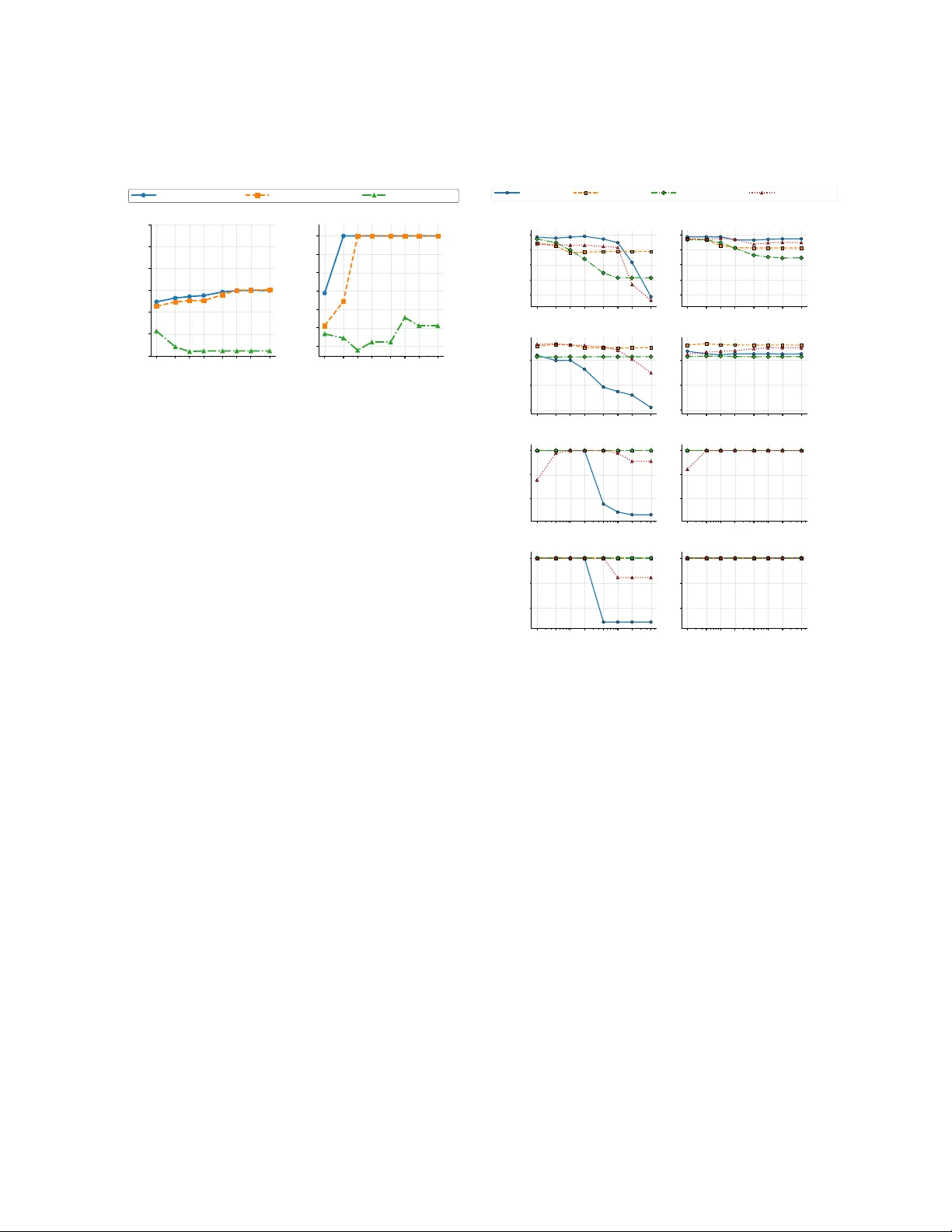
G AU S S I A N P R O C E S S L I M I T R E V E A L S S T RU C T U R A L B E N E FI T S O F G R A P H T R A N S F O R M E R S Nil A yday ∗ School of Computation, Information and T echnology T echnical Univ ersity of Munich nil.ayday@tum.de Lingchu Y ang ∗ Graduate School of Information Science and T echnology The Univ ersity of T okyo yang-lingchu@g.ecc.u-tokyo.ac.jp Debarghya Ghoshdastidar School of Computation, Information and T echnology T echnical Univ ersity of Munich March 19, 2026 A B S T R AC T Graph transformers are the state-of-the-art for learning from graph-structured data and are empirically kno wn to a void sev eral pitfalls of message-passing architectures. Howe ver , there is limited theoretical analysis on why these models perform well in practice. In this work, we pro ve that attention-based architectures hav e structural beneﬁts ov er graph con volutional networks in the context of node- lev el prediction tasks. Speciﬁcally , we study the neural network gaussian process limits of graph transformers (GA T , Graphormer , Specformer) with inﬁnite width and inﬁnite heads, and deri ve the node-lev el and edge-le vel k ernels across the layers. Our results characterise how the node features and the graph structure propagate through the graph attention layers. As a speciﬁc example, we pro ve that graph transformers structurally preserve community information and maintain discriminativ e node representations e ven in deep layers, thereby pre venting o versmoothing. W e provide empirical evidence on synthetic and real-w orld graphs that validate our theoretical insights, such as integrating informativ e priors and positional encoding can improv e performance of deep graph transformers. 1 Introduction Graph Neural Networks (GNNs) are currently the de facto models for learning from graph-structured data. They solve complex prediction tasks on graphs by iterati vely aggregating feature information across edges. Recent empirical and theoretical work has established that classical message-passing GNN architectures ha ve se veral limitations, including dif ﬁculties in simultaneously handling homophilic and heterophilic graphs [NT and Maehara, 2019, A yday et al., 2025], ov ersmoothing by deep GNNs [Li et al., 2018, K eri ven, 2022, W u et al., 2023b], o versquashing [Alon and Y ahav, 2021], etc. These challenges have moti vated the dev elopment of attention-based GNNs, such as Graph Attention Network (GA T) [V elicko vic et al., 2018], Graphormer [Y ang et al., 2021], and Specformer [Bo et al., 2023], which are the current state of the art models in practice. Despite the empirical success of graph transformers, there is little theoretical understanding of the beneﬁts of the attention mechanism in graph learning. The rich literature on the expressi vity of GNNs shows that transformers are more expressiv e than standard message-passing GNNs, but less expressiv e than more general message-passing architectures, like spectrally in v ariant GNNs [Zhang et al., 2024]. Howe ver , this line of work does not explain: Why do graph tr ansformers perform better with mor e layers and not suf fer fr om oversmoothing, similar to message-passing GNNs? Notably , oversmoothing —the phenomenon of node representations becoming indistinguishable in deeper layers—remains a topic of debate in recent theoretical works. W u et al. [2023a] use a dynamical system-based equiv alence of GA Ts to argue that they cannot pre vent oversmoothing, while a Markov chain perspective of GA Ts ∗ Equal contribution A P R E P R I N T - M A R C H 1 9 , 2 0 2 6 suggests their ability to mitigate ov ersmoothing Zhao et al. [2023]. Unlike GA T , which is limited to local neighborhoods, global attention-based models, like Graphormer and Specformer , allo w nodes to attend to all others, making them more complex to analyze, with no theoretical work currently a vailable. This lack of a uniﬁed theoretical lens for graph transformers leaves a fundamental question open: Can graph transformers over come the structural bottlenecks of message-passing , or do they mer ely delay the onset of oversmoothing? W e postulate that the abov e questions can be answered by studying the structural characteristics of graph transformers, speciﬁcally , how node r epr esentations evolve acr oss layers . T o this end, we utilize the framew ork of Neural Network Gaussian Processes (NNGPs), which establishes that randomly initialized neural networks con verge in distrib ution to Gaussian processes in the inﬁnite-width limit [Lee et al., 2018b]. The NNGP limit allows one to simplify GNNs, b ut still retain the architectural properties related to information aggreg ation and attention mechanism. In particular, recent works deri ve NNGP and related neural tangent limits of Graph Con v olutional Networks [Niu et al., 2023, Sabanayagam et al., 2023], which has also been used to characterize oversmoothing in these models. Howe ver , NNGP limits of graph transformers are not known. − 2 − 1 0 1 2 GNN Output − 30 − 25 − 20 − 15 − 10 − 5 0 log Density GA T: 1 Head 1000 Width − 1 . 0 − 0 . 5 0 . 0 0 . 5 1 . 0 GNN Output − 12 − 10 − 8 − 6 − 4 − 2 0 log Density GA T: 100 Heads 1000 Width − 4 − 2 0 2 4 GNN Output − 30 − 25 − 20 − 15 − 10 − 5 0 log Density Graphormer: 1 Head 1000 Width − 2 − 1 0 1 2 GNN Output − 12 − 10 − 8 − 6 − 4 − 2 0 log Density Graphormer: 100 Heads 1000 Width Figure 1: Histogram of the output of GA T and Graphormer for diff erent number of heads. The output distribution con- ver ges to a Gaussian (red line) ﬁtted with mean and v ariance of the empirical distrib ution when both width and number of heads are large. Plots for Specformer is in Appendix F. Contributions and signiﬁcance. The main technical con- tribution of this work is a deri vation of the NNGP k ernels for graph transformers, which we use to analytically sho w when these architectures can mitigate ov ersmoothing. W e brieﬂy discuss the signiﬁcance of the contributions. Derivation of NNGP kernel for graph tr ansformers. W e deriv e the NNGP limit of the three most relev ant graph transformer architectures (GA T , Graphormer , and Spec- former) and provide analytical forms of the kernel e volu- tion across layers for GA T -GP (Theorem 6), Graphormer- GP (Theorem 9), and Specformer-GP (Theorem 11). In contrast to previous work on GCN, where NNGP- equiv alence holds in the inﬁnite-width limit [Niu et al., 2023], transformer architectures behav e as NNGPs only when both the width and the number of heads are large (see Figure 1). Furthermore, unlike the NNGP limit of standard transformers [Hron et al., 2020], we show that graph transformers induce graph-speciﬁc kernels at multiple le vels—node-le vel kernels reﬂect the node feature interactions, whereas structural kernels capture connecti vity patterns, which correspond to edge-lev el ker - nels over graph neighborhoods in spatial models (GA T , Graphormer) and spectral kernels in spectral models (Specformer). These kernels interact non-trivially for various architectures (see T ables 1 – 2). Theor etical analysis of oversmoothing . T o study whether graph transformers mitigate ov ersmoothing, we simplify the NNGP kernels under the population version of (conte xtual) stochastic block model (CSBM), that is, graphs with well-deﬁned community structure. Our theoretical results, summarized in T able 3, conﬁrm that while GCN is structurally destined for oversmoothing, all attention-based GNNs can retain community information across layers under speciﬁc conditions. In particular , GA T -GP a voids rank collapse under well-separated communities, whereas Specformer -GP and Graphormer-GP counteract representational decay through spectral ampliﬁcation or informati ve structural priors. The analysis pro vides a crucial insight: if the NNGP limit of graph transformers does not ov ersmooth, then their neural architecture could potentially be trained to av oid ov ersmoothing noted in prior work [W u et al., 2023a]. Empirical validation of the impact of depth. W e v alidate our theoretical insights through numerical studies on synthetic and real-world benchmarks. As a practical consequence of our theory , we identify Laplacian-based positional encodings as a structural prior that prev ents ov ersmoothing in Graphormer-GP . Moreo ver , with a sufﬁciently informativ e structural prior , performance can e ven improv e as depth increases, which is unexpected in GCNs. 2 Preliminaries Notation. ⊙ denotes the Hadamard product, ∥ concatenation, and | · | 2 F the squared Frobenius norm, and tr( · ) the trace of a matrix. ϕ ( · ) is the row-wise softmax and σ ( · ) an arbitrary acti v ation function. 2 A P R E P R I N T - M A R C H 1 9 , 2 0 2 6 Graph Data. Let G = ( V , E ) be an undirected graph with n nodes, where V denotes the set of nodes and E the set of edges. Let A ∈ R n × n denote the adjacency matrix of the graph. The neighborhood of a node a ∈ V is deﬁned as N a := { i ∈ V | ( a, i ) ∈ E } . The d in -dimensional features for all N nodes are collected in rows of the n × d in matrix X , with the a -th row denoted by x ⊤ a . Graph Neural Networks (GNNs). GNNs are a class of deep learning models designed to learn node representations from graph-structured data by aggre gating information from local neighborhoods. S ( ℓ,h ) GNN ∈ R n × n denotes the graph con volution operator of head h in layer ℓ , whose form depends on the speciﬁc GNN architecture. For message-passing GNNs such as GCN, d ℓ,H = 1 and the graph con volution is ﬁxed, determined solely by the graph topology , giv en by S GCN = D − 1 / 2 AD − 1 / 2 . In comparison, graph transformers employ a data-dependent con volution in which neighborhood weights are learned via an attention mechanism. Giv en input features f 0 ( X ) := X , pre-activ ation of the ℓ -th layer is g ℓ ( X ) :=    d ℓ,H h =1 S ( ℓ,h ) GNN f ℓ − 1 ( X ) W ℓ,h  W ℓ,H , (1) where ∥ denotes concatenation of the attention heads and W ℓ,h ∈ R d ℓ − 1 × d ℓ and W ℓ,H ∈ R d ℓ − 1 d ℓ,H × d ℓ are learnable weight matrices. The layer output is obtained by applying a nonlinearity . ReLU acti vation is a common choice and is considered in this work: f ℓ ( X ) = ReLU  g ℓ ( X )  . Gaussian Process Limit of GNN Node Representations. W e analyse the node representations learned by GNNs through the lens of Neur al Network Gaussian Pr ocesses (NNGPs). In the inﬁnite-width and head limit, the model’ s pre-activ ations { g ℓ a ( X ) } a ∈ V con ver ge in distribution to a centered Gaussian process g ℓ ( X ) ∼ G P (0 , Σ ( ℓ ) ) . For ReLU activ ations ( f ℓ ( X ) = ReLU  g ℓ ( X )  ), the post-acti vation k ernel K ( ℓ ) admits a closed-form recursi ve update [Bietti and Mairal, 2019]: K ( ℓ ) ab = 1 2 π q Σ ( ℓ ) aa Σ ( ℓ ) bb  sin θ ( ℓ ) ab +  π − θ ( ℓ ) ab  cos θ ( ℓ ) ab  , θ ( ℓ ) ab = arccos   Σ ( ℓ ) ab q Σ ( ℓ ) aa Σ ( ℓ ) bb   . (2) Starting from the initial kernel K (0) ab := x a · x b d in , the sequence of kernels { Σ ( ℓ ) } ℓ ≥ 0 and { K ( ℓ ) } ℓ ≥ 0 are deﬁned recursi vely . Unlike standard NNGPs, in which the kernel is solely based on node features, the GNNs incorporate the graph structure and obtain predictions on unlabeled nodes by conditioning on observed node labels. In this work, we characterise the NNGP induced by graph transformers by deriving the corresponding cov ariance updates, thereby placing models such as GA T , Graphormer , and Specformer within a uniﬁed Gaussian process frame work. In the follo wing, we introduce graph transformers in vestigated in this paper: GA T , Graphormer , and Specformer . In contrast to these models, which operate on homogeneous graphs, the Graph T ransformer Network (GTN) is designed for heterogeneous graphs and is presented in Appendix D, including its model formulation, GP-equiv alent theorem, and proof. The design choices underlying GA T , Graphormer , and Specformer are detailed in Appendix A. Graph Attention Network (GA T). A multi-head GA T consists of d ℓ,H attention heads in layer ℓ . For each head h and layer ℓ , attention scores are computed on edges ( a, i ) ∈ E : E ( ℓh ) ai ( X ) =   v ℓh  ⊤  W ℓ,h f ℓ − 1 a ( X ) ∥ W ℓ,h f ℓ − 1 i ( X )  (3) where  v ℓh ∈ R 2 d ℓ × 1 is the attention vector . The normalized attention coefﬁcients are obtained via  S ( ℓ,h ) GA T ( X )  ai = exp  σ ( E ( ℓh ) ai ( X ))  P k ∈N a exp  σ ( E ( ℓh ) ak ( X ))  , (4) and  S ( ℓ,h ) GA T ( X )  ai = 0 for ( a, i ) / ∈ E . Graphormer . A Graphormer is a multi-head attention-based architecture with d ℓ,H heads in layer ℓ . Each layer augments node representations with graph positional encodings: ˜ f ℓ − 1 i ( X ) := [ f ℓ − 1 i ( X ) , P ℓ i ] for i ∈ V , where P ℓ i encodes structural information such as Laplacian eigen vectors, degree features, or random-walk-based statistics. For each head h and layer ℓ , attention scores are computed on all node pairs ( i, j ) ∈ V × V as E ( ℓh ) ij ( X ) =  ˜ f ℓ − 1 i ( X ) W Q,ℓh   ˜ f ℓ − 1 j ( X ) W K,ℓh  ⊤ √ d ℓ + b ρ ( i,j ) , (5) 3 A P R E P R I N T - M A R C H 1 9 , 2 0 2 6 where W Q,ℓh , W K,ℓh ∈ R d ℓ − 1 × d ℓ are learnable projection matrices, and the scaled dot-product term measures content- based compatibility between node i and node j . The additiv e bias b ρ ( i,j ) is a learnable scalar that depends only on the structural relation ρ ( · , · ) : V × V → R (e.g., shortest-path distance bucket, edge type, or other graph-structural categories). The graph con volution operator is obtained by applying the row-wise softmax, to the logits, i.e., S ( ℓ,h ) Graphormer ( X ) = ϕ  E ( ℓh ) ( X )  for head h . Specformer . Specformer operates on the spectrum of the normalized graph Laplacian: L := I n − D − 1 / 2 AD − 1 / 2 = U Λ U ⊤ with Λ = diag( λ 1 , . . . , λ n ) . Each eigenv alue λ i is encoded by a sinusoidal map ρ ( λ i ) ∈ R d with ρ ( λ, 2 t ) = sin  ϵλ/ 10000 2 t/d  , ρ ( λ, 2 t + 1) = cos  ϵλ/ 10000 2 t/d  and the initial spectral tokens are formed as H 0 = h ( λ 1 ∥ ρ ( λ 1 )) ⊤ , . . . , ( λ n ∥ ρ ( λ n )) ⊤ i ⊤ ∈ R n × ( d +1) . Consider a multi-head Specformer consisting of an eig en value encoding module with d t,H heads and a graph con volution module with d ℓ,H heads. For each graph con v olution head h ∈ { 1 , . . . , d ℓ,H } , the eigen value encoding module applies a d t,H -head attention at each eigen value encoding layer t , producing head-speciﬁc attention scores on token pairs ( i, j ) ∈ V × V : E ( t,k,h ) ij =  H t − 1 ,k,h i W Q,tkh  H t − 1 ,k,h j W K,tkh  ⊤ √ d t . (6) Here, k ∈ 1 , . . . , d t,H index es the attention head within token layer t , and W Q,tkh , W K,tkh ∈ R d t − 1 × d t are the corresponding projection matrices. The normalized attention coefﬁcients are given by S ( t,k,h ) Spec = ϕ  E ( t,k,h )  . The token-layer update for the h -th graph con volution head is H t,h =    d t,H k =1 S ( t,k,h ) Spec H t − 1 ,k,h W V ,tk h  W th,H , (7) where W V ,tk h ∈ R d t − 1 × d t is the v alue projection for the k -th eigen v alue encoding head and W t,H ∈ R d t,H d t × d t is the token-layer output projection. After T eigen v alue layers, the aggregated eigen v alue encoding output associated with the h -th graph con volution head is denoted by ¯ H ( h ) = H T ,h . The graph conv olution module then constructs a multi-head spectral ﬁltering operator . For each graph conv olution head h ∈ { 1 , . . . , d ℓ,H } , a spectral ﬁlter is generated by ¯ λ ( h ) = σ  ¯ H ( h ) W ( h ) λ  ∈ R n , where W ( h ) λ ∈ R d T × 1 is a learnable parameter v ector associated with the h -th graph con volution head. This induces the graph con volution operator S ( ℓ,h ) Specformer = U diag  ¯ λ ( h )  U ⊤ ∈ R n × n . 3 Gaussian process Limits of Graph T ransf ormers In this section, we analyse the GP limits of Graph Transformers architectures introduced in Section 2. W e begin by introducing the kernels that gov ern the Gaussian process limit and explain their roles, then present their explicit formulas in T able 1, and ﬁnally interpret their implications for the corresponding architectures in Section 3.1. Our analysis is carried out within the Neural Network Gaussian Process (NNGP) framew ork. Speciﬁcally , we characterise the behavior of GA T , Graphormer , and Specformer in the inﬁnite-width and inﬁnite-head limit , denoted as d ℓ , d ℓ,H → ∞ , and under the independent Gaussian priors listed in T able 4. In this regime, the models admit kernel recursions that go vern their layerwise propagation. In particular , we focus on the pre-acti vations g ℓ with k ernel Σ ( ℓ ) , and the post-acti vation k ernel K ( ℓ ) is obtained via the standard ReLU NNGP transformation (Equation 2). The complete theorems are provided in Appendix B. Spatial Models: GA T -GP and Graphormer -GP T o provide a uniﬁed analysis of GA T and Graphormer , we deﬁne four k ernels that gov ern the GP limit. These kernels model the propagation of information: we deﬁne the structural input (post-activ ation), model the attention mechanism (edge-lev el), aggregate these into a graph operator (con volution), and ﬁnally produce the node representations (node-le vel). T ogether , they form a recursion that characterizes the ev olution of graph signals through deep layers. • Post-Acti vation Ker nel of the Previous Layer: The propagation is initialized using the kernel from the previous iteration. For GA T , this is the post-activ ation kernel K ( ℓ − 1) . For Graphormer , this is the augmented ker nel ˜ K ( ℓ ) = αK ( ℓ − 1) + (1 − α ) R ( ℓ ) for α ∈ [0 , 1] , which incorporates structural positional encoding R ( ℓ ) . 4 A P R E P R I N T - M A R C H 1 9 , 2 0 2 6 T able 1: Summary of the GP kernels for graph transformers. The weight priors are in T able 4 in Appendix B. The table presents both the edge/structural kernels ( K ( ℓ ) ,E ab for spatial models or K λ,ab for Specformer) and the node-le vel kernels ( Σ ( ℓ ) ab ) that describe the propagation of cov ariance across layers. For GA T -GP and Graphormer-GP , the edge-lev el kernels capture correlations between attention scores, while the node-le vel k ernels aggregate these correlations. The learned spectral kernel K λ of Specformer-GP modulates the mapping of node representations in the Laplacian eigenbasis. Model Edge/Structural Ker nel ( K ( ℓ ) ,E ab or K λ ,ab ) Node Ker nel Σ ( ℓ ) ab GA T -GP (Theorem 6) σ 2 w σ 2 v  K ( ℓ − 1) ab + K ( ℓ − 1) ij  σ 2 H σ 2 w P i ∈ N a P j ∈ N b K ( ℓ − 1) ij C ( ℓ ) ai,bj Graphormer-GP (Theorem 9)  σ 2 Q σ 2 K ˜ K ( ℓ − 1) ab ˜ K ( ℓ − 1) ij + σ 2 b 1 ϕ ( a,i )= ϕ ( b,j )  σ 2 H σ 2 w P i,j ∈ V ˜ K ( ℓ − 1) ij C ( ℓ ) ai,bj Specformer-GP (Theorem 11) K λ,ab = E [ ¯ λ a ¯ λ b ] (Spectral) σ 2 H σ 2 w U ( K λ ⊙ ( U ⊤ K ( ℓ − 1) U )) U ⊤ • Edge-Level Logit Ker nel ( K ( ℓ ) ,E ): The attention logits E ( ℓ ) con ver ge to a centered Gaussian process E ( ℓ ) ∼ GP (0 , K ( ℓ ) ,E ) . This kernel describes the co variance between attention scores for dif ferent edges. • Con volution Ker nel ( C ( ℓ ) ): This kernel captures the cov ariance of the graph conv olution operator across independent heads and is deﬁned as C ( ℓ ) ai,bj := E h  S ( ℓ, 1) ( X )  ai  S ( ℓ, 1) ( X )  bj i . Its explicit form is determined by the Edge-Lev el Logit K ernel K ( ℓ ) ,E . • Node-Level K er nel ( Σ ( ℓ ) ): The ﬁnal cov ariance between node representations a and b after neighborhood aggregation, where Σ ( ℓ ) ab := E [ g ℓ a 1 ( X ) g ℓ b 1 ( X )] . Spectral Model: Specformer -GP Unlike spatial models, Specformer operates on the spectrum of L . Alongside the layerwise limits, when d t , d t,H → ∞ , the model con ver ges to a Gaussian process characterized by a set of kernels: • Spectral T oken Kernel: The representations of the t -th token layer , H ( t ) , conv erge in distribution to a Gaussian process H ( t ) ∼ GP (0 , K ( t ) H ) , which captures the evolution of spectral information through the eigen v alue encoding. • Learned Spectral Kernel ( K λ ): After T token layers, the learned spectral ﬁlter coefﬁcients ¯ λ , induces a kernel deﬁned as K λ,ab := E [ ¯ λ a ¯ λ b ] . • Node-Level Ker nel ( Σ ( ℓ ) ) This kernel propagates feature co v ariance by mapping previous-layer representa- tions into the Laplacian eigenbasis for elementwise modulation by the induced spectral kernel ( K λ ) before projecting them back to the node domain. The speciﬁc kernels for each architecture are summarized in T able 1. The independent Gaussian weight priors considered are summarized in T able 4 at the beginning of Appendix B. Formal theorems establishing the existence of the Gaussian process limits are provided in Appendix B, and detailed proofs of these theorems can be found in Appendix C. Explicit Ker nel Expressions. T able 1 summarizes a general k ernel recursion, which can be specialized by considering speciﬁc choices of the attention and activ ation nonlinearities to obtain a closed-form expressions. T able 2 presents the closed-form kernels obtained under linear attention (formally in Corollaries 8, and 10). For completeness, and to facilitate the comparison with attention-based architectures in the Section 4, we also include the corresponding GCN-GP kernel from [Niu et al., 2023], which does not incorporate attention mechanisms. These kernels provide a tractable way to study the GP limit under simpliﬁed attention and acti v ation choices, while still capturing the interaction between node features and graph structure. More general kernels can be obtained by considering RELU as output activ ation and applying Equation 2. In Appendix B Corollary 7, we also present GA T with RELU attention. 3.1 Remarks on GP ker nels The k ernels in T able 1 re v eal ho w node features and graph structure interact in the GP limit. In the following, we discuss the interpretation of these kernels in the graph domain and their implications for node representation propagation. 5 A P R E P R I N T - M A R C H 1 9 , 2 0 2 6 T able 2: Closed-form expressions for the node-lev el Gaussian process (GP) k ernels under linear attention and linear acti vation. These kernels pro vide an explicit characterization of kernel propagation for each architecture. For comparison, the GCN-GP kernel from [Niu et al., 2023] is included, which does not in volve attention. Model Node Ker nel ( K ( ℓ ) ) GCN-GP [Niu et al., 2023] K ( ℓ ) = σ 2 w AK ℓ − 1 A T GA T -GP (Corollary 8) K ( ℓ ) = σ 2 H σ 4 w σ 2 v  K ( ℓ − 1) ⊙ ( AK ( ℓ − 1) A ⊤ ) + A ( K ( ℓ − 1) ⊙ K ( ℓ − 1) ) A ⊤  Graphormer-GP (Corollary 10) K ( ℓ ) ab = σ 2 H σ 2 w " σ 2 Q σ 2 K ˜ K ( ℓ ) ab P i,j ∈ V ˜ K ( ℓ − 1) ij ˜ K ( ℓ − 1) ij + σ 2 b P i,j ∈ V ˜ K ( ℓ − 1) ij 1 ρ ( a,i )= ρ ( b,j ) # Specformer-GP (Theorem 11) K ( ℓ ) = σ 2 H σ 2 w U ( K λ ⊙ ( U ⊤ K ( ℓ − 1) U )) U ⊤ GA T -GP . The edge-level kernel K ( ℓ ) ,E of GA T -GP characterizes the cov ariance between attention logits on two edges ( a, i ) and ( b, j ) , determined by the similarity of their source nodes a and b and their target nodes i and j . Edges whose endpoints are simultaneously similar in representation space exhibit stronger correlation. The node-lev el kernel Σ ( ℓ ) then aggregates these edge contributions across all neighbor pairs ( i, j ) with i ∈ N a and j ∈ N b , combining the previous-layer feature similarity with the alignment induced by attention. This yields a kernel recursion describing how both features and graph structure gov ern node representation propagation across layers. Graphormer -GP Graphormer incorporates graph information through positional embeddings. The matrix R can be interpreted as the cov ariance matrix of the corresponding positional embeddings which can be computed as an inner product, i.e., R ( ℓ ) ab = ⟨ P ( ℓ ) a , P ( ℓ ) b ⟩ . Alternati vely , instead of introducing explicit positional embeddings, the graph structure itself can be directly le veraged to construct a node-lev el graph-structure cov ariance matrix. The node-level kernel Σ ( ℓ ) of Graphormer-GP indicates that attention correlations are strengthened for node pairs sharing the same structural relation, ensuring that graph information is explicitly le v eraged in guiding attention. The edge-lev el kernel K ( ℓ ) ,E then propagates the attention correlations to the next layer through an aggre gation ov er all node pairs. Unlike GA T which is restricted to local neighborhoods, Graphormer induces similarity connections between ev ery pair of nodes in the graph. Specformer . The con volution in Specformer is composed of spectr al tokens and node featur es . The spectral tokens are ﬁrst processed through T layers of encoding, and passed through a decoder to construct a data-dependent spectral ﬁltering that governs the propagation of node features. As detailed in Theorem 11 in Appendix B, (I) the spectral-token representations H t , which are updated through attention, and (II) the node-feature pre-acti v ations g ( X ) con ver ge in distribution to a Gaussian process. The learned spectral kernel K λ induces a kernel ov er the learned spectral ﬁlter coefﬁcients. The node le vel k ernel Σ l then deﬁnes the recursion of the node-feature kernel: the pre vious-layer node cov ariance is mapped into the Laplacian eigenbasis, modulated elementwise according to the induced spectral kernel, and projected back to the node domain. Spatial models aggregate information ov er local node neighborhoods, whereas Specformer operates in the graph spectral domain. 4 Analysis of GNN-GPs under Contextual Stochastic Block Model (CSBM) The GP formulation of graph transformers allows us to compare structural beneﬁts and limitations of different architectures. Having introduced k ernel recursion of graph transformers, we now focus on a k ey phenomenon in deep graph models: Oversmoothing . In the kernel perspecti ve, this corresponds to con ver gence of the node-lev el cov ariance tow ard a constant matrix. T o understand whether graph transformers can structurally maintain discriminativ e signals across layers, it is useful to study their GP kernels on a controlled setting with kno wn community structure. 6 A P R E P R I N T - M A R C H 1 9 , 2 0 2 6 In this section, we analyse how the resulting kernels behav e when the underlying graph is gov erned by a CSBM . W e consider population version of 2-CSBM with n nodes partitioned into two equally sized communities, C 1 and C 2 . In this setting, the probability of an edge existing between tw o nodes is p if they belong to the same community and q if they belong to different communities. The expected adjacency matrix takes the follo wing block structure: A =  p 11 ⊤ q 11 ⊤ q 11 ⊤ p 11 ⊤  , where 11 ⊤ denotes the all-ones matrix of size n 2 × n 2 2 . A kernel that captures the community structure should mirror this block structure, i.e. K ( ℓ ) =  x ℓ 11 ⊤ y ℓ 11 ⊤ y ℓ 11 ⊤ x ℓ 11 ⊤  , where x ℓ represents the kernel v alue for intra-community node pairs and y ℓ for inter-community pairs at layer ℓ , initialized by the feature cov ariance values x 0 and y 0 at the input layer ( ℓ = 0 ). While we analyse the population version, our experiments use random CSBM realizations, which exhibit similar behavior . W e summarise the ev olution of the kernels (formulas for x ℓ and y ℓ ) and their asymptotic behaviour in T able 3, highlighting how each model propagates structural information under the CSBM. The full corollaries and proofs for the closed-form expressions of the kernels are pro vided in Appendix E. T able 3: Evolution of the GP kernel K ( ℓ ) =  x ℓ 11 ⊤ y ℓ 11 ⊤ y ℓ 11 ⊤ x ℓ 11 ⊤  under CSBM and conditions f or oversmoothing . T o preserve community structure, the kernel must maintain a gap between the intra-community ( x ℓ ) and inter-community ( y ℓ ) v alues; this discriminativ e signal is captured by the second term in each e xpression.The second column indicates whether ov ersmoothing occurs as ℓ → ∞ , i.e., whether the kernel loses its ability to distinguish the two communities. For graph transformers o versmoothing can be a voided, maintaining the discriminati ve signal across layers. Model Intra/Inter -Community F ormulas ( x ℓ , y ℓ ) Oversmoothing ( ℓ → ∞ ) GCN-GP 1 2 ( n 2 ) 2 ℓ  ( x 0 + y 0 )( p + q ) 2 ℓ ± ( x 0 − y 0 )( p − q ) 2 ℓ  (Corollary 36) Y es (Corollary 1) GA T -GP 1 2 G 2 ℓ ( n 2 ) 2 ( p + q ) 2 h 1 ±  x 0 − y 0 x 0 + y 0  F ℓ i (Corollary 37) No, if communities are separated ( F ≥ 1 ) (Corollary 2) Graphormer-GP ˜ x ℓ = α ℓ x 0 + (1 − α ℓ ) p, ˜ y ℓ = α ℓ y 0 + (1 − α ℓ ) q (Corollary 38) No, if the prior ( R ) captures communities (Remark 3) Specformer-GP 1 2  ( x 0 + y 0 ) ¯ λ 2 ℓ 1 ± ( x 0 − y 0 ) ¯ λ 2 ℓ 2  (Corollary 39) No, if | ¯ λ 2 | ≥ | ¯ λ 1 | (Remark 5) Oversmoothing can be formalized by examining the normalized kernel K ( ℓ ) 1 n tr ( K ( ℓ ) ) . Since the normalisation term corresponds to x ℓ , the discriminability of the model is captured by the ratio y ℓ /x ℓ : if lim ℓ →∞ y ℓ /x ℓ = 1 , the kernel con ver ges to a rank-one matrix of ones, meaning the representations of the two communities become indistinguishable. GCN. The collapse into a rank-one kernel is clearly visible in the Gaussian Process limit of standard GCN. Corollary 1 (Rank collapse in GCN-GP indicates oversmoothing) . F or the GCN kernel pr esented in Cor ollary 36 (and in T able 3). The normalized kernel con ver ges to the all-ones matrix: lim ℓ →∞ K ( ℓ ) 1 n tr ( K ( ℓ ) ) =  11 ⊤ 11 ⊤ 11 ⊤ 11 ⊤  . Consequently , rank  lim ℓ →∞ K ( ℓ ) 1 n tr ( K ( ℓ ) )  = 1 , indicating that GCNs suffer fr om complete oversmoothing. The detailed deri vations for the closed-form expressions of the GCN kernel and the spectral analysis leading to rank collapse are provided in Appendix E.1. GA T . Unlike the GCN kernel, which collapses to a rank-one matrix, we next sho w that GA T -GP a voids o versmoothing. Notably , while the GCN kernel follows a simple linear recurrence, the GA T kernel in volv es a coupled, non-linear two-v ariable system. The deriv ation of the GA T kernel under SBM (Corollary 37) and its limit (Corollary 2) are provided in Appendix E.2. The GA T kernel is governed by the global growth factor G = ( x 0 + y 0 )( p + q ) 2 ( n 2 ) 2 2 Throughout this section, SBM refers to the two-community stochastic block model introduced abov e. 7 A P R E P R I N T - M A R C H 1 9 , 2 0 2 6 and the structural preser vation factor F = 2 p 2 − pq + q 2 ( p + q ) 2 . Here, G controls the ov erall magnitude of the kernel, while F determines whether the community structure is preserved across layers. In particular , when the communities are sufﬁciently well-separated, F ensures that the kernel maintains its ability to distinguish between them e ven in the inﬁnite-depth limit. This property is formalised in the follo wing corollary: Corollary 2 (GA T -GP avoids rank collapse indicating the preservation of discriminativ e community struc- ture) . F or the GA T kernel deﬁned in Cor ollary 37, the normalized k ernel conver ges to: lim ℓ →∞ K ( ℓ ) 1 n tr ( K ( ℓ ) ) =  11 ⊤ γ 11 ⊤ γ 11 ⊤ 11 ⊤  , wher e γ = lim ℓ →∞ 1 −  x 0 − y 0 x 0 + y 0  F ℓ 1+  x 0 − y 0 x 0 + y 0  F ℓ . Consequently , if F ≥ 1 , which occurs when p q is bounded away fr om 1, the kernel maintains a rank of 2 and pr eserves community separation as ℓ → ∞ , avoiding oversmoothing . Graphormer . Consider the Graphormer kernel from Corollary 10 in Appendix B without the bias term, and assume that the positional encodings capture all structural information of the graph. In the SBM setting, this implies that the spatial relation matrix coincides with the adjacency matrix, i.e., R = A . Under SBM, the block entries ˜ x ℓ and ˜ y ℓ of ˜ K ( ℓ ) are determined by the recurrence giv en in T able 3. The normalized kernel from T able 2 without the bias term can be written as K ( ℓ ) = ˜ K ( ℓ ) · Z ℓ − 1 , with Z ℓ − 1 = tr ( A ⊤ ( ˜ K ( ℓ − 1) ⊙ ˜ K ( ℓ − 1) )) . Since our analysis focuses on whether the kernel preserves the block structure induced by the SBM, the trace term does not play a role. Consequently , it sufﬁces to study the ev olution of ˜ K ( ℓ ) . Remark 3 (Graphormer Con vergence) . As the number of layers ℓ → ∞ , the unnormalized Graphormer kernel ˜ K ( ℓ ) con ver ges to the spatial r elation matrix R . In the SBM setting wher e R = A , the kernel effectively r ecovers the gr ound truth, impr oving its ability to distinguish communities with incr easing depth. This beneﬁt, however , r elies entir ely on the quality of the positional encodings; in a r eal-world dataset if R is uninformative, the kernel may collapse towar d a non-discriminative prior , r esulting in oversmoothing . Specformer . The e volution of the Specformer kernel under SBM is presented in T able 3. Unlike the GCN and Graphormer kernels, the Specformer uses a learnable spectral ﬁlter, which is characterised by the parameters ¯ λ 1 and ¯ λ 2 that determine the cross-co v ariance K λ (Equation 33). These eigen values control ho w dif ferent spectral components are ampliﬁed across layers, and therefore determine whether the kernel preserves the block structure induced by the SBM. Depending on the choice of ¯ λ 1 and ¯ λ 2 , Specformer can either collapse to the GCN beha viour or maintain community separation, as detailed in the following remarks. Remark 4 (Specformer Collapses to GCN) . The Specformer-GP kernel collapses to the GCN-GP kernel if the learned spectral weights corr espond to the eigen values of the adjacency matrix, i.e ., ¯ λ 1 = n 2 ( p + q ) and ¯ λ 2 = n 2 ( p − q ) . In this case, the Specformer kernel e xhibits the same oversmoothing behaviour (Cor ollary 1). Remark 5. Specformer can pr eserve community structur e, even in the limit ℓ → ∞ , when the learned spectr al ﬁlter satisﬁes | ¯ λ 2 | ≥ | ¯ λ 1 | , as this ampliﬁes the spectral dir ection that carries the community information. Summary of Oversmoothing Beha vior While GCN-GP is structurally destined for rank collapse and oversmoothing, attention-based models provide mechanisms to preserve structural information. GA T -GP a voids o versmoothing under a data-dependent condi- tion: communities need to be sufﬁ ciently separated, which is a standard expectation for graph learning tasks. Graphormer-GP relies on a prior that encodes meaningful structural information to prev ent ov ersmoothing. In contrast, Specformer-GP offers a learnable solution, where avoiding oversmoothing is determined by the spectral weights optimized during training rather than by the data or prior . T ogether, these ﬁndings highlight how architectural design inﬂuence o versmoothing. 5 Discussions and Experiments While graph transformers are notoriously difﬁcult to analyse due to complex attention mechanisms and training dynamics, our Gaussian Process (GP) framework provides a mathematically rigorous closed-form equiv alent. W e provide the ﬁrst kernel equi valent for graph transformers, thereby offering a tool for studying their structural properties. A structural phenomenon we in vestigate is ov ersmoothing . In Section 4, we formalise this behaviour by analysing GP kernels under CSBM, re vealing a fundamental distinction: while GCN-GP is destined to oversmooth (Corollary 1), attention-based architectures can preserve discriminati ve community representations as depth increases. Consistent with this theory , e valuating GP kernels on synthetic and benchmark datasets (homophilic Pubmed [Sen et al., 2008] and heterophilic Chameleon [Rozemberczki et al., 2019]) shows that GCN-GP performance deteriorates with depth , 8 A P R E P R I N T - M A R C H 1 9 , 2 0 2 6 whereas GA T -GP remains resilient to oversmoothing (Figure 3, left; Corollary 2). Details of the experiments are provided in Appendix F, and the code to reproduce the experiments is a v ailable at https://figshare.com/s/ 4ad5245d4d6c405f46f0 . 2 5 10 20 50 100 200 500 0 . 4 0 . 5 0 . 6 0 . 7 0 . 8 0 . 9 1 . 0 Chameleon 2 5 10 20 50 100 200 500 0 . 4 0 . 5 0 . 6 0 . 7 0 . 8 0 . 9 1 . 0 SBM (random features) Number of Lay ers T est Accuracy Laplacian Eigenvectors Spectral Reconstruction Centralit y Enco ding Figure 2: Oversmoothing behaviour and the impact of positional encodings. T est accuracy of Graphormer - GP on Chameleon (left) and SBM with random features (right) as a function of the number of layers. While accuracy in graph models typically suffers from perfor- mance degradation with an increasing number of layers, Graphormer -GP exhibits increasing accuracy with depth when utilizing informati ve positional encodings, such as Laplacian Eigenv ectors (blue) and Spectral Re- construction (orange). This empirical trend aligns with the theoretical results in Corollary 3. 2 5 10 20 50 100 200 500 0 . 4 0 . 5 0 . 6 0 . 7 0 . 8 Pubmed T est Accuracy 2 5 10 20 50 100 200 500 0 . 4 0 . 5 0 . 6 0 . 7 0 . 8 2 5 10 20 50 100 200 500 0 . 2 0 . 4 0 . 6 Chameleon T est Accuracy 2 5 10 20 50 100 200 500 0 . 2 0 . 4 0 . 6 2 5 10 20 50 100 200 500 0 . 6 0 . 8 1 . 0 SBM (random features) T est Accuracy 2 5 10 20 50 100 200 500 0 . 6 0 . 8 1 . 0 2 5 10 20 50 100 200 500 0 . 6 0 . 8 1 . 0 CSBM (aligned features) T est Accuracy 2 5 10 20 50 100 200 500 0 . 6 0 . 8 1 . 0 Original Model with Laplacian Eigenvectors Number of Layers GCN-GP GA T-GP Specformer-GP Graphormer-GP Figure 3: Oversmoothing behaviour across various GNN-GP architectures. T est accuracy is shown as a function of depth for the original models (left) and mod- els augmented with Laplacian Eigen vectors (right). In the original conﬁgurations, GCN-GP (blue) consistently suffers from a performance drop-off as the number of layers incr eases . In contrast, GA T -GP (orange) demonstrates resilience to depth , maintaining stable performance as argued in Corollary 2. The behavior of Specformer-GP and Graphormer-GP depends on the dataset. Notably , upon incorporating Laplacian Eigen vec- tors (right), the tendency to oversmooth is signiﬁcantly mitigated across all architectures. Graphormer -GP is sensitive to structural prior . Re- mark 3, argues that when the structural prior is informati ve, Graphormer beneﬁts from depth, as the kernel con ver ges tow ard the spatial relation matrix (e.g., the ground-truth adjacency in SBM). Ho wev er , when an informativ e struc- tural prior is not e xplicitly kno wn for a real-world dataset, Graphormer may still suffer from ov ersmoothing as the ker- nel collapses toward a non-discriminative prior . Since Graphormer can incorporate dif ferent structural priors, we ran additional e xperiments on SBM with random features and Chameleon. W e ev aluate three positional encodings (without bias) at large depth (Figure 5): Laplacian Eigen- vectors , Spectral Reconstruction (lo w-rank Laplacian ap- proximation), and Centrality Encoding (from Y ang et al. [2021]). Across both datasets, Laplacian-based encodings outperform centrality encoding and resist oversmoothing. Moti vated by these results, we incorporate Laplacian Eigen- vectors into the other GP architectures (Figure 3, right) and ﬁnd that they can mitigate the onset of o versmoothing. Broader P erspective The GP equiv alence for graph transformers established in this work pro vides a foundation for a broader theoretical analysis. Analysing the model in the inﬁnite-width regime, independent of training dynamics, yields corresponding kernel equi valents that enable the study of structural properties. Among the central questions in such analyses is expressi vity , as the model’ s representational power can be characterised by the expressi vity of the corresponding kernel. While our current analysis demonstrates community separation at large depth in the CSBM setting, it can be extended to study other critical structural phenomena, including oversquashing (the bottleneck of information propagation) and the model’ s sensitivity to heter ophily under more complex random graph models. GP equiv alence has already successfully enabled the study of generalisation [Seeger, 2003] and inducti ve biases [Li et al., 2021] in deep learning. This work provides the ﬁrst uniﬁed theoretical lens based on GP for graph transformers, laying the foundation for a deeper understanding of graph attention mechanisms. 9 A P R E P R I N T - M A R C H 1 9 , 2 0 2 6 References Uri Alon and Eran Y ahav . On the bottleneck of graph neural networks and its practical implications. In 9th International Confer ence on Learning Repr esentations, 2021 , 2021. Nil A yday , Mahalakshmi Sabanayagam, and Debar ghya Ghoshdastidar . Why does your graph neural network fail on some graphs? insights from exact generalisation error . CoRR , abs/2509.10337, 2025. Alberto Bietti and Julien Mairal. On the inductiv e bias of neural tangent kernels. In Advances in Neural Information Pr ocessing Systems , 2019. Patrick Billingsle y . Pr obability and Measure . W iley , 2 edition, 1986. J. R. Blum, J. Kiefer , and M. Rosenblatt. Distribution free tests of independence based on the sample distribution function. Annals of Mathematical Statistics , 29:485–498, 1958. Deyu Bo, Chuan Shi, Lele W ang, and Renjie Liao. Specformer: Spectral graph neural networks meet transformers. In The Eleventh International Confer ence on Learning Representations, ICLR , 2023. Adrià Garriga-Alonso, Carl Edward Rasmussen, and Laurence Aitchison. Deep con volutional networks as shallow gaussian processes. In International Confer ence on Learning Repr esentations (ICLR) , 2019. Jiri Hron, Y asaman Bahri, Jascha Sohl-Dickstein, and Roman Nov ak. Inﬁnite attention: NNGP and NTK for deep attention networks. In Proceedings of the 37th International Confer ence on Machine Learning (ICML) , Proceedings of Machine Learning Research (PMLR), 2020. Nicolas Keri ven. Not too little, not too much: a theoretical analysis of graph (over)smoothing. In Sanmi Koyejo, S. Mohamed, A. Agarwal, Danielle Belgrav e, K. Cho, and A. Oh, editors, Advances in Neural Information Pr ocessing Systems 35: Annual Confer ence on Neural Information Pr ocessing Systems 2022, NeurIPS 2022, New Orleans, LA, USA, November 28 - December 9, 2022 , 2022. Jaehoon Lee, Y asaman Bahri, Roman Nov ak, Samuel S. Schoenholz, Jascha Sohl-Dickstein, and Jef frey Pennington. Deep neural networks as gaussian processes. In International Conference on Learning Repr esentations (ICLR) , 2018a. Jaehoon Lee, Jascha Sohl-dickstein, Jef frey Pennington, Roman No vak, Sam Schoenholz, and Y asaman Bahri. Deep neural networks as gaussian processes. In International Confer ence on Learning Repr esentations , 2018b. Michael Y . Li, Erin Grant, and Thomas L. Grif ﬁths. Meta-learning inducti ve biases of learning systems with gaussian processes. In Fifth W orkshop on Meta-Learning at the Conference on Neur al Information Pr ocessing Systems , 2021. Qimai Li, Zhichao Han, and Xiao-Ming W u. Deeper insights into graph con v olutional networks for semi-supervised learning. In Pr oceedings of the Thirty-Second AAAI Confer ence on Artiﬁcial Intelligence, (AAAI-18) , 2018. Alexander G. de G. Matthews, Jiri Hron, Mark Ro wland, Richard E. T urner, and Zoubin Ghahramani. Gaussian process behaviour in wide deep neural netw orks. In International Conference on Learning Repr esentations (ICLR) , 2018. Zehao Niu, Mihai Anitescu, and Jie Chen. Graph neural network-inspired kernels for gaussian processes in semi- supervised learning. In The Eleventh International Confer ence on Learning Repr esentations, ICLR , 2023. Roman Nov ak, Lechao Xiao, Y asaman Bahri, Jaehoon Lee, Greg Y ang, Jeffrey Pennington, and Jascha Sohl-Dickstein. Bayesian deep con volutional netw orks with many channels are gaussian processes. In International Confer ence on Learning Repr esentations (ICLR) , 2019. Hoang NT and T akanori Maehara. Revisiting graph neural netw orks: All we hav e is low-pass ﬁlters. CoRR , 2019. Benedek Rozemberczki, Ryan Davies, Rik Sarkar, and Charles Sutton. GEMSEC: Graph embedding with self clustering. In Pr oceedings of the IEEE/A CM International Confer ence on Advances in Social Networks Analysis and Mining (ASON AM) , pages 65–72, 2019. Mahalakshmi Sabanayag am, P ascal Mattia Esser , and Debar ghya Ghoshdastidar . Analysis of con volutions, non-linearity and depth in graph neural networks using neural tangent kernel. T rans. Mach. Learn. Res. , 2023, 2023. Matthias W . Seeger . Pac-bayesian generalisation error bounds for gaussian process classiﬁcation. J. Mac h. Learn. Res. , pages 233–269, 2003. Prithviraj Sen, Galileo Namata, Mustafa Bilgic, Lise Getoor , Brian Galligher, and T ina Eliassi-Rad. Collectiv e classiﬁcation in network data. AI Magazine , 29(3):93–106, 2008. Petar V elickovic, Guillem Cucurull, Arantxa Casanov a, Adriana Romero, Pietro Liò, and Y oshua Bengio. Graph attention networks. In 6th International Confer ence on Learning Repr esentations , 2018. Xiao W ang, Houye Ji, Chuan Shi, Bai W ang, Peng Cui, Philip S. Y u, and Y anfang Y e. Heterogeneous graph attention network. arXiv pr eprint arXiv:1903.07293 , 2019. 10 A P R E P R I N T - M A R C H 1 9 , 2 0 2 6 Xinyi W u, Amir Ajorlou, Zihui W u, and Ali Jadbabaie. Demystifying ov ersmoothing in attention-based graph neural networks. In Advances in Neural Information Pr ocessing Systems 36: Annual Confer ence on Neural Information Pr ocessing Systems 2023 , 2023a. Xinyi W u, Zhengdao Chen, W illiam W ei W ang, and Ali Jadbabaie. A non-asymptotic analysis of o versmoothing in graph neural networks. In The Eleventh International Confer ence on Learning Repr esentations , 2023b. Greg Y ang. Scaling limits of wide neural networks with weight sharing: Gaussian process behavior , gradient indepen- dence, and neural tangent kernel. arXiv preprint, 2019. Junhan Y ang, Zheng Liu, Shitao Xiao, Chaozhuo Li, Defu Lian, Sanjay Agrawal, Amit Singh, Guangzhong Sun, and Xing Xie. Graphformers: Gnn-nested transformers for representation learning on textual graph. In Advances in Neural Information Pr ocessing Systems 34: Annual Confer ence on Neural Information Pr ocessing Systems , 2021. Bohang Zhang, Lingxiao Zhao, and Haggai Maron. On the expressiv e power of spectral in v ariant graph neural networks. In Ruslan Salakhutdinov , Zico Kolter , Katherine A. Heller , Adrian W eller , Nuria Oliv er , Jonathan Scarlett, and Felix Berkenkamp, editors, F orty-ﬁrst International Confer ence on Machine Learning, ICML 2024, V ienna, Austria, J uly 21-27, 2024 , v olume 235 of Pr oceedings of Machine Learning Resear ch , pages 60496–60526. PMLR / OpenRevie w .net, 2024. W eichen Zhao, Chenguang W ang, Congying Han, and T iande Guo. Exploring over -smoothing in graph attention networks from the marko v chain perspecti ve. In Pr oceedings of the International Confer ence on F r ontiers of Artiﬁcial Intelligence and Machine Learning , F AIML , 2023. 11 A P R E P R I N T - M A R C H 1 9 , 2 0 2 6 A Design Choices A.1 GNN with Multi-Head Aggregation A common ﬁnite-head formulation aggregates H = d ℓ,H head outputs by concatenation: f ℓ ( X ) =    d ℓ,H h =1 σ  S ( ℓ,h ) GNN f ℓ − 1 ( X ) W ℓ,h  , (8) where ∥ denotes concatenation. This formulation is not suitable for taking the limit d ℓ,H → ∞ , since concatenation leads to an ev er-gro wing output dimension and prevents a CL T -based inﬁnite-head analysis. T o obtain a well-deﬁned inﬁnite-head limit in a ﬁxed feature dimension, we modify the aggregation mechanism by introducing a shared projection that aggregates all head-wise outputs into the ne xt-layer representation: f ℓ ( X ) = σ     d ℓ,H h =1 S ( ℓ,h ) GNN f ℓ − 1 ( X ) W ℓ,h  W ℓ,H  , (9) where W ℓ,h are head-speciﬁc weight matrices and W ℓ,H is a shared projection mapping the concatenated head outputs to the ﬁxed-dimensional feature space of layer ℓ . This modiﬁcation plays a crucial role in the inﬁnite-head analysis: it replaces dimension gro wth by a ﬁxed-dimensional linear aggregation of head-wise random features, which enables a CL T -type argument despite the n × n stochasticity of S ( ℓ,h ) GNN ( X ) and the induced dependence across coordinates. As a result, the inﬁnite-head GNN in (9) admits a principled Gaussian-process limit while retaining the expressi ve stochastic message-passing structure encoded by S ( ℓ,h ) GNN . A.2 Graphormer In the original Graphormer architecture, structural information is injected through a centrality encoding , where each node representation is augmented by learnable embeddings indexed by its in-degree and out-de gree. Using our notation, the input node representation can be written as f (0) i ( X ) = x i + z deg − ( v i ) + z deg + ( v i ) , (10) where x i denotes the raw node feature and z deg − , z deg + ∈ R d are learnable degree-based embeddings. For undirected graphs, the two degree terms are uniﬁed into a single de gree encoding. While such a design ef fectiv ely injects node importance signals into the attention mechanism and has demonstrated strong empirical performance on graph-le vel tasks, it represents a speciﬁc instance of structural augmentation based solely on degree statistics. This degree-centric formulation becomes restrictiv e when considering node-lev el prediction tasks or when aiming to incorporate richer and more general notions of graph structure. T o generalize this mechanism, we reinterpret centrality encoding as a special case of feature-le vel graph encoding insertion. Instead of restricting the structural signal to degree-based embeddings, we introduce a general graph encoding term P ℓ i at layer ℓ , and deﬁne the augmented node representation as ˜ f ℓ i ( X ) :=  f ℓ i ( X ) , P ℓ i  , i ∈ V , (11) where f ℓ i ( X ) denotes the node representation produced by the backbone network at layer ℓ , and P ℓ i ∈ R d p encodes structural or positional information associated with node v i . More importantly , (11) allows P ℓ i to represent arbitrary graph encodings, including but not limited to Laplacian positional encodings, random w alk-based encodings, or other task-speciﬁc structural descriptors. By explicitly separating semantic features f ℓ i ( X ) from structural encodings P ℓ i , the proposed formulation provides a ﬂexible and general mechanism for injecting graph structure into the model. This is particularly advantageous for node-le vel tasks, where the prediction target depends on ﬁne-grained local and mesoscopic structural patterns rather than global graph summaries. Furthermore, the concatenation-based design preserves the modularity of the architecture and facilitates theoretical analysis, as dif ferent choices of P ℓ i can be studied independently of the backbone representation. In summary , we treat centrality encoding as a special case of a more general graph encoding frame work. The uniﬁed representation (11) enables the incorporation of di verse structural signals in a principled manner , while maintaining compatibility with T ransformer-based architectures and node-le vel prediction settings. 12 A P R E P R I N T - M A R C H 1 9 , 2 0 2 6 A.3 Specformer Spectral Graph Construction in Specformer . In the original Specformer model, the graph structure is learned in the spectral domain through a set of spectral tokens. Let H t ∈ R n × d ℓ,H denote the spectral tokens at layer t in eigen v alue encoding, where each column corresponds to the output of one attention head. At layer t, each attention head h = 1 , . . . , d ℓ,H produces a separate spectral representation via Z h = A ttention  H t W Q,th , H t W K,th , H t W V ,th  , (12) where W Q,th , W K,th , and W V ,th are learnable projection matrices. The head-speciﬁc representation Z h is then mapped to a vector of ﬁltered eigen values, λ h = σ ( Z h W λ ) ∈ R N , (13) where σ ( · ) denotes an acti v ation function. Each eigen v alue vector λ h deﬁnes a spectral graph operator S h = U diag( λ h ) U ⊤ , (14) with U denoting the eigen vector matrix of the graph Laplacian. As a result, the d ℓ,H attention heads produce d ℓ,H distinct spectral graph operators { S h } d t,H h =1 . These operators are subsequently used as intermediate bases to construct feature-wise graph structures. Speciﬁcally , the operators are concatenated along the channel dimension and mapped to the node feature dimension d through a feed-forward netw ork (FFN), ˆ S = FFN  [ I N ∥ S 1 ∥ · · · ∥ S d t,H ]  ∈ R N × N × d . (15) The output ˆ S thus consists of d graph operators, where each slice ˆ S : , : ,i corresponds to a distinct adjacenc y (or Laplacian) matrix associated with the i -th node feature dimension. Based on these feature-wise graph operators, graph con volution is performed independently for each feature channel. Let f ( X ) ( ℓ − 1) ∈ R N × d denote the node representations at layer ℓ − 1 . For the i -th feature dimension, the propagation is giv en by ˆ f ( X ) ( ℓ − 1) : ,i = ˆ S : , : ,i f ( X ) ( ℓ − 1) : ,i , (16) and the node representations are updated as f ( X ) ( ℓ ) = σ  ˆ f ( X ) ( ℓ − 1) W ( ℓ − 1)  . (17) While this construction is e xpressi ve, it introduces a fundamental statistical issue. Since the d graph operators { ˆ S : , : ,i } d i =1 are jointly generated through a shared FFN, the y are statistically dependent. Consequently , the feature dimensions of ˆ f ( ℓ ) ( X ) are no longer independent, violating the independence assumptions required by the Central Limit Theorem (CL T). As a result, the original Specformer formulation does not satisfy the conditions necessary for CL T -based inﬁnite-width analysis. Multi-head Aggregated Spectral Construction. T o address this issue, for each head of graph con volution layer heads d ℓ,H , we modify the spectral construction by employing multi-head attention to generate a single set of spectral coefﬁcients, rather than one per feature dimension. Speciﬁcally , at each layer t , the outputs of the d t,H spectral heads are aggregated prior to spectral ﬁltering. The spectral tokens are updated as H t +1 =    d t,H h =1 S ( t,h ) Spec  H t  H t W V ,th  W H,t , (18) where W H,t is a learnable projection matrix. After T eigen v alue encoding layers, we obtain the ﬁnal spectral tokens ¯ H = H T . Based on ¯ H , a single set of spectral coefﬁcients is generated as ¯ λ = σ  ¯ H W λ  ∈ R n , (19) which deﬁnes the ﬁnal graph con volution operator S Specformer = U diag( ¯ λ ) U ⊤ ∈ R n × n . (20) By constructing a shared spectral operator across feature dimensions, this formulation preserves feature-wise indepen- dence and restores the conditions required for CL T -based inﬁnite-width analysis. 13 A P R E P R I N T - M A R C H 1 9 , 2 0 2 6 T able 4: Summary of the Gaussian weight priors used for each graph transformer in the GP analysis. These priors deﬁne the variance of the initial weights for all linear transformations and attention parameters. Model W eight Priors (V ariance) GA T W ℓ,H ij ∼ N  0 , σ 2 H d ℓ,H d ℓ − 1  , W ℓ,h ij ∼ N  0 , σ 2 w d ℓ − 1  ,  v ℓh k ∼ N  0 , σ 2 v d ℓ − 1  Graphormer W Q,ℓh ij ∼ N  0 , σ 2 Q d ℓ − 1  , W K,ℓh ij ∼ N  0 , σ 2 K d ℓ − 1  , W ℓ,H ij ∼ N  0 , σ 2 H d ℓ,H d ℓ − 1  , W V ,ℓh ij ∼ N  0 , σ 2 w d ℓ − 1  , b ρ ( i, j ) ∼ N (0 , σ 2 b ) Specformer W Q,tkh ij ∼ N (0 , σ 2 Q /d t − 1 ) , W K,tkh ij ∼ N (0 , σ 2 K /d t − 1 ) , W V ,tkh ij ∼ N (0 , σ 2 V /d t − 1 ) , W th,H ij ∼ N  0 , σ 2 O d t,H d t − 1  , B F ormal Theorems on Gaussian Pr ocess Limits of Graph T ransformers In this Appendix, we present the formal theorems and kernel recursions establishing the Gaussian process limits for graph transformers, deriv ed under the independent Gaussian weight priors summarized in T able 4. Graph Attention Network (GA T) In GA T , attention is computed locally o ver graph neighborhoods, and in the inﬁnite-width and inﬁnite-head limit, both the attention logits and node pre-activ ations con ver ge to Gaussian processes. The resulting kernel recursion re veals ho w features and neighborhood structure jointly shape representation propagation. Theorem 6. (Inﬁnite-width and inﬁnite-head limit of a GA T layer) Assume that the parameters of the ℓ -th GA T layer satisfy W ℓ,H ij ∼ N  0 , σ 2 H d ℓ,H d ℓ − 1  , W ℓ,h ij ∼ N  0 , σ 2 w d ℓ − 1  ,  v ℓh k ∼ N  0 , σ 2 v d ℓ − 1  , independently for all i, j, k and heads h , then, as d ℓ , d ℓ,H → ∞ , the following holds: (I) E ℓ ( X ) =  E ( ℓh ) ( X ) : h ∈ N  con ver ges in distrib ution to E ℓ ( X ) ∼ G P (0 , K ( ℓ ) ,E ) with K ( ℓh ) ,E ai,bj = E  E ( ℓh ) ai ( X ) E ( ℓh ′ ) bj ( X )  = δ h = h ′ σ 2 w σ 2 v  K ( ℓ − 1) ab + K ( ℓ − 1) ij  , (21) (II) g ℓ ( X ) con verges in distrib ution to g ℓ ( X ) ∼ G P (0 , Σ ( ℓ ) ) with C ( ℓ ) ai,bj := E h  S ( ℓ, 1) GA T ( X )  ai  S ( ℓ, 1) GA T ( X )  bj i = E h ϕ  σ ( E ( ℓ 1) ai ( X ))  ϕ  σ ( E ( ℓ 1) bj ( X ))  i , (22) Σ ( ℓ ) ab := E  g ℓ a 1 ( X ) g ℓ b 1 ( X )  = σ 2 H σ 2 w X i ∈ N a X j ∈ N b K ( ℓ − 1) ij C ( ℓ ) ai,bj , (23) wher e a, b ∈ V and ( a, i ) , ( b, j ) ∈ E . Theorem 6 sho ws that, for each attention head, the collection of attention logits ov er edges con ver ges in distribution to a centered Gaussian process, with dif ferent heads becoming independent in the limit. Equation (21) characterizes the cov ariance between attention logits on two edges ( a, i ) and ( b, j ) , which is dri ven by the similarity between the two source nodes a, b together with the similarity between the two target nodes i, j , so edges whose endpoints are simultaneously close in representation space e xhibit stronger correlation. Using Equation (21) , the theorem then deri ves the Gaussian process limit of the pre-activ ations. Equation (23) describes ho w node-lev el dependence propagates to the next layer , where the covariance between the pre-acti v ations of nodes a and b at layer ℓ is obtained by aggregating contributions from all neighbor pairs ( i, j ) with i ∈ N a and j ∈ N b , combining similarity among neighboring node representations from the pre vious layer with the alignment induced by attention on the associated edges. T ogether , these results yield a kernel recursion that describes ho w feature and graph go vern representation propagation across layers. Theorem 6 establishes a general kernel recursion, and to obtain a closed-form recursion, we next consider speciﬁc choices of the attention and activ ation nonlinearities. Corollary 7. (Closed-form GA T kernel recur sion) Under the assumptions of Theor em 6, for ϕ ( x ) = x and ReLU activation σ ( · ) , the node-level covariance k ernel at layer ℓ admits the closed-form expr ession Σ ( ℓ ) ab = σ 2 H σ 4 w σ 2 v 2 π X i ∈ N a X j ∈ N b K ( ℓ − 1) ij × q  K ( ℓ − 1) aa + K ( ℓ − 1) ii  K ( ℓ − 1) bb + K ( ℓ − 1) j j  ×  sin θ ( ℓ − 1) ai,bj +  π − θ ( ℓ − 1) ai,bj  cos θ ( ℓ − 1) ai,bj  . (24) 14 A P R E P R I N T - M A R C H 1 9 , 2 0 2 6 θ ( ℓ − 1) ai,bj = arccos   K ( ℓ − 1) ab + K ( ℓ − 1) ij q  K ( ℓ − 1) aa + K ( ℓ − 1) ii  K ( ℓ − 1) bb + K ( ℓ − 1) j j    . (25) K ernel in Corollary 7 induces a quadratic computational cost ov er neighborhood pairs. T o further simplify the recursion, we consider a linear activ ation. Corollary 8 (Linear GA T kernel) . Under the assumptions of Corollary 7, and for σ ( x ) = x , the node-level kernel admits the following simpliﬁed closed-form r ecursion: Σ ( ℓ ) = σ 2 H σ 4 w σ 2 v  K ( ℓ − 1) ⊙  AK ( ℓ − 1) A ⊤  + A  K ( ℓ − 1) ⊙ K ( ℓ − 1)  A ⊤  . Graphormer As introduced in Section 2, Graphormer incorporates graph information through a positional encoding mechanism. In the inﬁnite-width limit, the output conv erges in distrib ution to a Gaussian process whose kernel satisﬁes ˜ K ( ℓ − 1) 7− → α K ( ℓ − 1) + (1 − α ) R ( ℓ ) , α ∈ (0 , 1) . (26) Where the matrix R can be interpreted as the covariance matrix of the corresponding positional encoding which can be computed as an inner product of positional embeddings, i.e., R ( ℓ ) ab = ⟨ P ( ℓ ) a , P ( ℓ ) b ⟩ . Alternati vely , instead of introducing explicit positional embeddings, the graph structure itself can be directly lev eraged to construct a node-lev el graph-structure cov ariance matrix. Theorem 9 characterizes the Gaussian process limit of a Graphormer layer by establishing joint limits for both the attention logits and the node pre-activ ations. Although the proof strategy is analogous to GA T , the incorporation of positional encodings and ho w the attention scores are computed modiﬁes the kernel. Centrality Encoding (CE) differs from other positional encoding that it constructs a learnable embedding based on node degrees. Speciﬁcally , a CE parameter matrix has size P CE ∈ R ( max_degree +1) × d , and each entry is initialized as ( P CE ) ij ∼ N  0 , σ 2 CE d  . Since we only consider undirected graphs in this paper, nodes with the same degree share the same embedding vector , i.e., P v = P CE [deg( v )] ∈ R d . Under this construction, the embedding correlation satisﬁes E  P ⊤ a P b  =  σ 2 CE , deg ( a ) = deg( b ) , 0 , deg( a )  = deg ( b ) . Therefore, we obtain R ab =  σ 2 CE , deg ( a ) = deg( b ) , 0 , deg( a )  = deg ( b ) . Theorem 9. (Inﬁnite-width and inﬁnite-head limit of a Graphormer layer) Assume the parameters of the ℓ -th Graphormer layer satisfy W Q,ℓh ij ∼ N  0 , σ 2 Q d ℓ − 1  , W K,ℓh ij ∼ N  0 , σ 2 K d ℓ − 1  , W ℓ,H ij ∼ N  0 , σ 2 H d ℓ,H d ℓ − 1  , W V ,ℓh ij ∼ N  0 , σ 2 w d ℓ − 1  , b ϕ ( i, j ) ∼ N (0 , σ 2 b ) , independently for all i, j , heads h , and structural indices ϕ ( i, j ) , then, as d ℓ , d ℓ,H → ∞ , the following holds: (I) E ℓ ( X ) =  E ( ℓh ) ( X ) : h ∈ N  con ver ges in distrib ution to E ℓ − 1 ( X ) ∼ G P (0 , K ( ℓ ) ,E ) with K ( ℓh ) ,E ai,bj = E  E ( ℓh ) ai ( X ) E ( ℓh ′ ) bj ( X )  = δ h = h ′  σ 2 Q σ 2 K ˜ K ( ℓ − 1) ab ˜ K ( ℓ − 1) ij + σ 2 b 1 ϕ ( a,i )= ϕ ( b,j )  . (27) (II) g ℓ ( X ) con verges in distrib ution to g ℓ ( X ) ∼ G P (0 , Σ ( ℓ ) ) with C ( ℓ ) ai,bj := E h  S ( ℓ, 1) Graphormer ( X )  ai  S ( ℓ, 1) Graphormer ( X )  bj i = E h ϕ  E ( ℓ 1) ai ( X )  ϕ  E ( ℓ 1) bj ( X )  i , (28) Σ ( ℓ ) ab := E  g ℓ a 1 ( X ) g ℓ b 1 ( X )  = σ 2 H σ 2 w X i ∈ V X j ∈ V ˜ K ( ℓ − 1) ij C ( ℓ ) ai,bj , (29) wher e a, b, i, j ∈ V . 15 A P R E P R I N T - M A R C H 1 9 , 2 0 2 6 Equation (26) shows that the ef fectiv e similarity between nodes depends on both the similarity of node features and the similarity of graph structural features encoded by the positional information. Equation (27) further indicates that attention correlations are strengthened for node pairs sharing the same structural relation, ensuring that graph information is explicitly leveraged in guiding attention. Equation (29) then propagates the attention correlations to the next layer through an aggregation over all node pairs, reﬂecting that, unlike GA T which is restricted to local neighborhoods, Graphormer induces similarity connections between e very pair of nodes in the graph. The following corollary specializes Theorem 9 to linear attention. Corollary 10 (Closed-form Graphormer k ernel under linear attention) . Under the assumptions of Theorem 9, and for ϕ ( x ) = x , Consequently , the node-level covariance kernel at layer ℓ admits the closed-form expr ession Σ ( ℓ ) ab = σ 2 H σ 2 w " σ 2 Q σ 2 K ˜ K ( ℓ − 1) ab X i,j ∈ V ˜ K ( ℓ − 1) ij ˜ K ( ℓ − 1) ij + σ 2 b X i,j ∈ V ˜ K ( ℓ − 1) ij 1 ϕ ( a,i )= ϕ ( b,j ) # , where a, b, i, j ∈ V . Specformer . As detailed in Section 2, the con volution in Specformer is composed of spectral tokens and node featur es . The spectral tokens are ﬁrst processed through T layers of encoding, and are subsequently passed through a decoder to construct a data-dependent spectral ﬁltering that go verns the propag ation of node features. The following theorem characterizes the beha vior of Specformer in the inﬁnite-width and inﬁnite-head limit. In this re gime, (I) the spectral- token representations H t , which are updated through attention, and (II) the node-feature pre-activ ations g ( X ) con ver ge in distribution to a Gaussian process. Theorem 11. (Inﬁnite-width and inﬁnite-head limit of Specformer) If the parameters of the t -st token layer satisfy W Q,tkh ij ∼ N (0 , σ 2 Q /d t − 1 ) , W K,tkh ij ∼ N (0 , σ 2 K /d t − 1 ) , W V ,tk h ij ∼ N (0 , σ 2 V /d t − 1 ) and W th,H ij ∼ N  0 , σ 2 O d t,H d t − 1  , independently for all indices, token heads k , and spectral heads h , then, as d t , d t,H → ∞ , the following holds. (I) H t con ver ges in distrib ution to H t ∼ G P (0 , K ( t ) H ) with K ( t,k,h ) ,E ik,j l = E h E ( t,k,h ) ij ( H ) E ( t,k ′ ,h ′ ) kl ( H ′ ) i = δ k = k ′ δ h = h ′ σ 2 Q σ 2 K K ( t − 1) H,ik K ( t − 1) H,j l , (30) C ( t,h ) ik,j l ( H, H ′ ) := δ h = h ′ E h  S ( t, 1 ,h ) Spec ( H )  ik  S ( t, 1 ,h ′ ) Spec ( H ′ )  j l i = δ h = h ′ E h ϕ  E ( t, 1 ,h ) ik ( H )  ϕ  E ( t, 1 ,hi ) j l ( H ′ )  i , (31) K ( t,h ) H,ij := E  ( H t,h ) i ( H t,h ′ ) j  = δ h = h ′  σ 2 O σ 2 V X k,l ∈ V K ( t − 1) H,kl C ( t,h ) ik,j l ( H, H ′ )  , (32) wher e i, k , j, l ∈ V and K (0 ,h ) H,ab := H 0 a · H 0 b d with d as the spectral-token embedding dimension. (II) If the parameters of the ℓ -st graph con volution layer satisfy W ℓ,ij ∼ N (0 , σ 2 w /d ℓ − 1 ) , W ℓ,H ij ∼ N  0 , σ 2 H d ℓ,H d ℓ − 1  and the eigen value decoder layers satisfy W ( ℓ,h ) λ,ij ∼ N (0 , σ 2 λ /d T ) independently for all indices and spectr al heads h , then, as d ℓ , d T , d ℓ,H → ∞ , g ℓ ( X ) con verges in distrib ution to G P (0 , Σ ( ℓ ) ) with K λ,ab := δ h = h ′ E  ¯ λ ( h ) a ( H ) ¯ λ ( h ′ ) b ( H ′ )  = δ h = h ′ E h σ  ( ¯ H ( h ) W ( ℓ,h ) λ ) a  σ  ( ¯ H ( h ′ ) W ( ℓ,h ) λ ) b  i , (33) Σ ( ℓ ) ab = σ 2 H σ 2 w U  K λ ⊙  U ⊤ K ( ℓ − 1) U   U ⊤ , (34) wher e a, b ∈ V . Equations (30) – (32) describe ho w the co variance induced by the previous token layer is recursi vely transformed through a standard transformer . At the terminal token layer , Equation (33) transfers the resulting token-lev el cov ariance to the spectral domain by inducing a kernel ov er the learned spectral ﬁlter coef ﬁcients. Equation (34) then deﬁnes the 16 A P R E P R I N T - M A R C H 1 9 , 2 0 2 6 recursion of the node-feature kernel: the previous-layer node cov ariance is mapped into the Laplacian eigenbasis, modulated elementwise according to the induced spectral kernel, and projected back to the node domain. T ogether , these equations specify a coupled kernel recursion in which attention gov erns spectral reweighting, and graph con volution propagates the resulting cov ariance across layers. C Proofs of Theor ems 6, 9, 11, 34 Proof technique. Our analysis follo ws the standard induction-on-layers framework for establishing Gaussian process (GP) limits of randomly initialized deep neural architectures (Matthe ws et al. [2018], Lee et al. [2018a], Nov ak et al. [2019], Garriga-Alonso et al. [2019], Y ang [2019], Hron et al. [2020]). When the layer - ( ℓ − 1) representations con v erge in distrib ution to a Gaussian process, we show that the layer- ℓ representations also conv erge to a Gaussian process under suitable initialization and moment conditions. A ke y methodological step of this work is to dev elop a uniﬁed con v ergence frame work for graph transformers in the inﬁnite-head regime. At a high level, our strate gy is to establish a single inﬁnite-head con vergence theorem that yields a Gaussian-process limit for the model outputs, while making explicit the analytic conditions required for interchanging limits and expectations. Concretely , Appendix C.1 proves a general inﬁnite-head con vergence result for multi-head attention aggregation layers, cov ering all four architectures studied in this paper within one theorem. Importantly , this output-le vel con vergence in the inﬁnite-head limit is not obtained in isolation: the proof requires distributional con ver gence of the corresponding graph con volution operators, together with uniform integrability , which ensures con ver gence of expectations and justiﬁes interchanging limits and E [ · ] . Therefore, we separately establish the con vergence of the graph con volution operators for each model Appendix C.2, C.3, C.4, and D. These operator -lev el results, together with uniform integrability (Lemma 27), yield con ver gence of expectations via Theorem 28. Combining these ingredients completes a single coherent route to the ﬁnal, uniform con ver gence statements for all models under inﬁnitely many heads. T echnically , the core con ver gence arguments proceed by reducing ﬁnite-dimensional distributional claims to one- dimensional linear projections via the Cramér–W old device (Lemma 26), followed by a central limit theorem for exchangeable triangular arrays (Lemma 12) applied at the multi-head aggregation le vel. Slutsky’ s lemma (Lemma 29) and the continuous mapping theorem are then used to combine the con ver gent random components. Finally , passage of limits through expectations is justiﬁed by uniform integrability (Lemma 27) together with the conv ergence-of- expectations theorem (Theorem 28), which is enabled precisely by the inte grability properties established through the graph con volution operator con vergence in Appendix C.2 – D. C.1 Conv ergence of g ℓ ( X ) Since all this four models require the number of attention heads to grow to inﬁnity in order to admit a well-deﬁned Gaussian Process (GP) limit, we adopt a uniﬁed and general analytical framew ork to establish their GP con ver gence. W e analyze the multi-head aggre gation at a ﬁx ed layer inde x ℓ , mapping the GP input f ℓ − 1 to the GP output f ℓ . For each head h ∈ { 1 , . . . , d ℓ,H } , node a ∈ V and input X ∈ X 0 , deﬁne the single-head pre-activ ation output at layer ℓ by g ℓh ( X ) := S ( ℓ,h ) GNN f ℓ − 1 ( X ) W ℓ,h , (35) The multi-head output at layer ℓ is giv en by g ℓ ( X ) =  g ℓ 1 ( X ) , . . . , g ℓd ℓ,H ( X )  W ℓ,H , (36) where W ℓ,H is the output projection matrix, whose columns we write as W ℓ,H =  w ℓ,H 1 , . . . , w ℓ,H d ℓ,H  , with w ℓ,H h corresponding to head h . The v ariance of W ℓ,H is chosen such that the overall scaling corresponds to a properly rescaled weighted sum ov er the d ℓ,H attention heads. Lemma 12 (Adaptation of Theorem 2 from Blum et al., 1958) . F or each m ∈ N , let { X m,i : i = 1 , 2 , . . . } be an inﬁnitely exc hangeable sequence with E [ X n, 1 ] = 0 and E [ X 2 m, 1 ] = σ 2 n , such that lim m →∞ σ 2 m = σ 2 for some σ 2 ≥ 0 . Let S n = 1 √ d m d m X i =1 X m,i , (37) 17 A P R E P R I N T - M A R C H 1 9 , 2 0 2 6 for some sequence ( d m ) m ≥ 1 ⊂ N such that lim m →∞ d m = ∞ . Assume: ( a ) E [ X m, 1 X m, 2 ] = 0 , ( b ) lim n →∞ E [ X 2 m, 1 X 2 m, 2 ] = σ 4 , ( c ) E | X m, 1 | 3 = o ( p d m ) . Then S n d − → Z , wher e Z = 0 if σ 2 = 0 , and Z ∼ N (0 , σ 2 ) otherwise. Lemma 13 (Node-le vel GP limit) . Let the assumptions of Theorem 6 , Theor em 9, Theor em 11 and Theor em 34 hold. The collection of layer- ℓ pre-activation outputs g ℓ ( X ) :=  g ℓ a ( X ) : X ∈ X 0 , a ∈ V  con ver ges in distribution to a centr ed Gaussian pr ocess whose ﬁnite-dimensional marginals ar e Gaussian with covariance given by the node-level k ernel K ( ℓ ) . Pr oof. Follo wing the Cramér–W old device [Billingsley, 1986, p. 383], it sufﬁces to establish con vergence of one- dimensional projections of ﬁnite-dimensional marginals of g ℓ ( X ) . Fix a ﬁnite index set L ⊂ X 0 × V and test vectors { α X,a ∈ R N : ( X, a ) ∈ L} . Consider the linear statistic T ( ℓ ) := X ( X,a ) ∈L ( α X,a ) ⊤ g ℓ a ( X ) . (38) Using the concatenation form (36) and writing g ( ℓ +1) h a ( X ) for the a -th ro w of the h -th head, we obtain T ( ℓ ) = X ( X,a ) ∈L ( α X,a ) ⊤  d ℓ,H X h =1 g ℓh a ( X ) w ℓ,H h  = d ℓ,H X h =1 X ( X,a ) ∈L ( α X,a ) ⊤ g ℓh a ( X ) w ℓ,H h | {z } =: ζ h . Deﬁne the rescaled head-lev el v ariables ψ h := √ d ℓ,H ζ h , h = 1 , . . . , d ℓ,H , so that T ( ℓ ) = 1 √ d ℓ,H d ℓ,H X h =1 ψ h . (39) For each head width d ℓ,H , this deﬁnes a triangular array { ψ d ℓ,H ,h } d ℓ,H h =1 , where, suppressing the explicit dependence on d ℓ,H for notational simplicity , each ψ h admits the representation ψ h = √ d ℓ,H X ( X,a ) ∈L ( α X,a ) ⊤ g ℓh a ( X ) w ℓ,H h . (40) Thus T ( ℓ ) is of the form (37) in Lemma 12, with X n,i identiﬁed with ψ h and d n with d ℓ,H . T o in v oke Lemma 12, it sufﬁces to v erify conditions (a)–(c) for the array { ψ h } d ℓ,H h =1 , which is achiev ed by the follo wing lemmas: • Exchangeability of { ψ h } in the head index h is established in Lemma 14. • Zero mean and vanishing cross-co variance, E [ ψ 1 ] = 0 and E [ ψ 1 ψ 2 ] = 0 , follow from Lemm a 15. • Con ver gence of the variance, E [ ψ 2 1 ] → τ 2 , is prov ed in Lemma 16. • Con ver gence of the mixed fourth moment E [ ψ 2 1 ψ 2 2 ] → τ 4 and the gro wth condition E | ψ 1 | 3 = o ( √ d ℓ,H ) are established in Lemma 17. 18 A P R E P R I N T - M A R C H 1 9 , 2 0 2 6 Therefore, by Lemma 12, T ( ℓ ) con ver ges in distribution to a centred Gaussian random variable with v ariance τ 2 . Since L and the test vectors { α X,a } are arbitrary , the ﬁnite-dimensional distributions of g ℓ ( X ) con ver ge to those of a Gaussian process with cov ariance gi ven by the node-le vel kernel K ( ℓ ) . □ Lemma 14 (Head-wise e xchangeability) . Under the assumptions of Theor em 6, the r andom variables { ψ h } d ℓ,H h =1 ar e exc hangeable over the head inde x h . Pr oof. In all four of our models, for distinct heads h , the parameters { W ℓ,h , w ℓ,H h } (including those appearing in S ( ℓ,h ) GNN ) are i.i.d. across h and independent of all pre vious-layer variables. Conditioning on the pre vious-layer representation f ℓ − 1 ( · ) (i.e., ﬁxing { f ℓ − 1 ( x ) : x ∈ X } ), (40) implies that ( ψ 1 , . . . , ψ d ℓ,H ) are i.i.d. in h , and hence their conditional joint distribution is in variant under an y permutation of the head indices. Therefore, by de Finetti’ s theorem, { ψ h } h ∈ N is inﬁnitely exchangeable. Lemma 15 (Head-wise zero mean and vanishing cross-co v ariance) . E [ ψ 1 ] = E [ ψ 1 ψ 2 ] = 0 . Pr oof. From (40), ψ 1 = X ( X,a ) ∈L √ d ℓ,H ( α X,a ) ⊤  S ( ℓ, 1) GNN f ℓ ( X )  a w ℓ,H 1 . Condition on the σ -algebra generated by { f ℓ ( X ) : X ∈ X 0 } and { S ( ℓ,h ) GNN : h ∈ N } . Under this conditioning, w ℓ,H 1 is independent of all conditioned variables and is centred Gaussian. Therefore, E h ψ 1    { f ℓ ( X ) } X ∈X 0 , { S ( ℓ,h ) GNN } h ∈ N i = X ( X,a ) ∈L √ d ℓ,H ( α X,a ) ⊤  S ( ℓ, 1) GNN f ℓ ( X )  a E [ w ℓ,H 1 ] = 0 , and hence E [ ψ 1 ] = 0 . For E [ ψ 1 ψ 2 ] , expand the product using (40): ψ 1 ψ 2 = d ℓ,H X ( X,a ) ∈L X ( X ′ ,b ) ∈L ( α X,a ) ⊤  S ( ℓ, 1) GNN f ℓ ( X )  a ( α X ′ ,b ) ⊤  S ( ℓ, 2) GNN f ℓ ( X ′ )  b w ℓ,H 1 w ℓ,H 2 . Conditioning on { f ℓ ( X ) } X ∈X 0 and { S ( ℓ,h ) GNN } h ∈ N , the random variables w ℓ,H 1 and w ℓ,H 2 are independent, centred Gaussian and independent of the remaining factors in each summand. Thus E [ w ℓ,H 1 w ℓ,H 2 ] = E [ w ℓ,H 1 ] E [ w ℓ,H 2 ] = 0 , which implies E h ψ 1 ψ 2    { f ℓ ( X ) } X ∈X 0 , { S ( ℓ,h ) GNN } h ∈ N i = 0 , and hence E [ ψ 1 ψ 2 ] = 0 . Lemma 16 (Head-wise variance con vergence) . There e xists τ 2 ≥ 0 such that lim d ℓ,H →∞ E [ ψ 2 1 ] = τ 2 . Pr oof. Observe that E [ ψ 2 1 ] can be written as E [ ψ 2 1 ] = d ℓ,H X ( X,a ) , ( X ′ ,b ) ∈L ( α X,a ) ⊤ E h g ℓ 1 ( X ) w ℓ,H 1 w ℓ,H 1 ⊤ g ℓ 1 ( X ′ ) ⊤ i α X ′ ,b σ 2 H d ℓ X ( X,a ) , ( X ′ ,b ) ∈L ( α X,a ) ⊤ E h g ℓ 1 ( X ) g ℓ 1 ( X ′ ) ⊤ i α X ′ ,b , where we used E [ w ℓ,H 1 w ℓ,H 1 ⊤ ] = σ 2 H d ℓ d ℓ,H . 19 A P R E P R I N T - M A R C H 1 9 , 2 0 2 6 σ 2 H d ℓ E h g ℓ 1 ( X ) g ℓ 1 ( X ) ⊤ i = σ 2 H d ℓ E h  S ( ℓ, 1) GNN f ℓ − 1 ( X ) W ℓ, 1   S ( ℓ, 1) GNN f ℓ − 1 ( X ) W ℓ, 1  ⊤ i = σ 2 H E h S ( ℓ, 1) GNN f ℓ − 1 ( X ) f ℓ − 1 ( X ) ⊤ d ℓ − 1 ( S ( ℓ, 1) GNN ) ⊤ i W e may thus apply Lemma 28, which requires con v ergence in distrib ution of the inte grands to the rele vant limit and uniform integrability of the integrand family . Con ver gence in distribution follo ws by combining the model-speciﬁc con ver gence argument in Lemma 18, Lemma 24, Lemma 25, Lemma 35 with Lemma 29 and Hron et al. [2020, Lemma 33] combined continuous mapping theorem. Uniform integrability is obtained by Hölder’ s inequality together with Hron et al. [2020, Lemma 32] and the corresponding moment propagation result for S ( ℓ,h ) GNN , namely Lemma 30, Lemma 31,Lemma 32, Lemma 33 . Hence the integrand family is uniformly integrable by Lemma 27, concluding the proof. Lemma 17. F or any h, h ′ ∈ N , E [ ψ 2 h ψ 2 h ′ ] con ver ges to the mean of the weak limit of { ψ 2 h ψ 2 h ′ } d ℓ,H →∞ . Pr oof. It is enough to prove con vergence of e xpectations of the form E h g ℓh a ( X ) g ℓh b ( X ′ ) ⊤ g ℓh ′ c ( Y ) g ℓh ′ d ( Y ′ ) ⊤ i , where a, b, c, d range over feature indices and ( X, X ′ , Y , Y ′ ) ∈ L . Using the deﬁnition of g ℓh , we may rewrite the abo ve as E h g ℓh a ( X ) g ℓh b ( X ′ ) ⊤ g ℓh ′ c ( Y ) g ℓh ′ d ( Y ′ ) ⊤ i = σ 4 w E h  S ( ℓ,h ) GNN  a f ℓ − 1 ( X ) f ℓ − 1 ( X ′ ) ⊤ d ℓ − 1  S ( ℓ,h ) GNN  b  S ( ℓ,h ′ ) GNN  c f ℓ − 1 ( Y ) f ℓ − 1 ( Y ′ ) ⊤ d ℓ − 1  S ( ℓ,h ′ ) GNN  d i . By Hron et al. [2020, Lemma 33],  f ℓ − 1 ( X ) f ℓ − 1 ( X ′ ) ⊤ d ℓ − 1 , f ℓ − 1 ( Y ) f ℓ − 1 ( Y ′ ) ⊤ d ℓ − 1  P − →  K ( ℓ − 1) ( X, X ′ ) , K ( ℓ − 1) ( Y , Y ′ )  . Since S ( ℓ,h ) GNN and S ( ℓ,h ′ ) GNN con ver ge in distrib ution (and are independent of the weight matrices producing f ℓ − 1 ). Then the entire integrand con ver ges in distribution by Lemma 29. Finally , Billingsley [1986, Theorem 3.5] together with Hölder’ s inequality and Hron et al. [2020, Lemma 32] implies uniform integrability of the integrand f amily and hence con ver gence of the expectation, concluding the proof. C.2 Conv ergence of S ( ℓ,h ) GA T In Lemma 13, we sho wed that, under the GP induction hypothesis on the node features, it is sufﬁcient to assume that S ( ℓ,h ) GNN con ver ges in distribution in order for the layer- ( ℓ ) pre-activ ation outputs g ℓ ( X ) to con ver ge in distribution to a Gaussian process. In the standard GA T parameterisation, S ( ℓ,h ) GNN is a measurable function of the attention logits E ( ℓh ) , and hence con ver gence of E ( ℓh ) to a centred Gaussian process implies con vergence of S ( ℓ,h ) GNN by the continuous mapping theorem. Consequently , to establish Gaussian process con vergence of the GA T outputs, it suf ﬁces to prov e that the attention logits con ver ge in distribution to a centred Gaussian process. W e no w recall the version of the Blum–Kiefer –Rosenblatt central limit theorem that we will use, follo wing Matthews et al. [2018, lemma 10], and apply it to establish con ver gence of the attention logits. Fix a layer index ℓ . For each head h and graph edge ( a, i ) ∈ E , recall the attention logit E ( ℓh ) ai ( X ) :=  v ⊤ ℓh  W ℓ,h f ℓ a ( X ) , W ℓ,h f ℓ i ( X )  , with the scaling and independence assumptions on W ℓ,h and  a ℓh giv en in Theorem 6. 20 A P R E P R I N T - M A R C H 1 9 , 2 0 2 6 Because the graph structure in GA T only affects the model through subsequent linear aggregation of the attention outputs, and linear transformations preserve Gaussianity , it suf ﬁces to establish con ver gence of the attention logits themselves. More precisely , for the ﬁxed layer ℓ , we show that the collection of logits E ( ℓ ) :=  E ( ℓh ) ai ( X ) : X ∈ X 0 , ( a, i ) ∈ E , h ∈ N  has ﬁnite-dimensional marginals con ver ging, as d ℓ → ∞ , to those of a centred process with cov ariance giv en by the edge-lev el kernel K ( ℓ ) ,E deﬁned in Equation (21) of Theorem 6. Lemma 18 (Logit-lev el GP limit of GA T) . Let the assumptions of Theorem 6 hold. Then, for the ﬁxed layer ℓ , the pr ocess E ( ℓ ) :=  E ( ℓh ) ai ( X ) : X ∈ X 0 , ( a, i ) ∈ E , h ∈ N  con ver ges in distribution (as d ℓ → ∞ ) to a centr ed process whose ﬁnite-dimensional marginals ar e Gaussian with covariance given by the edge k ernel K ( ℓ ) ,E of (21) in Theor em 6. Pr oof. Using Hron et al. [2020, Lemma 27] and the Cramér–W old de vice [Billingsley, 1986], we may restrict attention to one-dimensional projections of ﬁnite-dimensional marginals of E ( ℓ ) . Let C ⊂ X 0 × E × N be ﬁnite, and choose test matrices { β X,ai,h } of the same shape as E ( ℓh ) ai ( X ) . W e consider linear statistics of the form T E ℓ := X ( X, ( a,i ) ,h ) ∈C  β X,ai,h , E ( ℓh ) ai ( X )  F = X ( X, ( a,i ) ,h ) ∈C * β X,ai,h , 1 √ d ℓ d ℓ X j =1 h  v ( L ) ℓh,j W ℓ,h, · j f ℓ − 1 a ( X ) · 1 ⊤ + 1 ·  v ( R ) ℓh,j W ℓ,h, · j f ℓ − 1 i ( X ) i + F = 1 √ d ℓ d ℓ X j =1 X ( X, ( a,i ) ,h ) ∈C  β X,ai,h ,  v ( L ) ℓh,j W ℓ,h, · j f ℓ − 1 a ( X ) · 1 ⊤ + 1 ·  v ( R ) ℓh,j W ℓ,h, · j f ℓ − 1 i ( X )  F | {z } =: φ j . Here ⟨· , ·⟩ F denotes the Frobenius inner product (equiv alently , the Euclidean inner product on vectorised matrices). W e decompose the vector v into two subvectors v ( L ) and v ( R ) , which have equal length and identical distribution. Thus T E ℓ is of the form (37) with X n,i identiﬁed with φ j and d n with d ℓ . T o inv oke Lemma 12 it sufﬁces to verify conditions (a)–(c) for { φ j } d ℓ j =1 , which we do in Lemmas 19 – 23 below: • Exchangeability in j is established in Lemma 19. • Zero mean and vanishing cross-co variance follo w from Lemma 20. • Con ver gence of the variance is established in Lemma 21. • Con ver gence of E [ φ 2 1 φ 2 2 ] is proved in Lemma 22. • The o ( √ d ℓ ) growth of the third absolute moment is implied by Lemma 23. Hence T E ℓ con ver ges in distribution to a centred Gaussian random v ariable with variance determined by the limit of E [ φ 2 1 ] , which is exactly the cov ariance speciﬁed by the edge-le vel kernel K ( ℓh ) ,E . Since C and the test coefﬁcients are arbitrary , the claim follows by Cramér –W old. □ Lemma 19 (Exchangeability over feature index) . Under the assumptions of Theorem 6, the random variables { φ j } d ℓ j =1 ar e exc hangeable over the inde x j . Lemma 20 (Zero mean and vanishing cross-co v ariance) . Under the assumptions of Theorem 6, we have E [ φ 1 ] = 0 , E [ φ 1 φ 2 ] = 0 . Pr oof. Recall that, for a ﬁnite index set C ⊂ X 0 × E × N , φ j = X ( X, ( a,i ) ,h ) ∈C  β X,ai,h ,  v ( L ) ℓh, 1 W ℓ,h, · 1 f ℓ − 1 a ( X ) · 1 ⊤ + 1 ·  v ( R ) ℓh, 1 W ℓ,h, · 1 f ℓ − 1 i ( X )  F , j = 1 , 2 , where ⟨· , ·⟩ F is the Frobenius inner product. 21 A P R E P R I N T - M A R C H 1 9 , 2 0 2 6 Mean. For an y ﬁxed ( X, ( a, i ) , h ) ∈ C , E h  β X,ai,h ,  v ( L ) ℓh, 1 W ℓ,h, · 1 f ℓ a ( X ) · 1 ⊤ + 1 ·  v ( R ) ℓh, 1 W ℓ,h, · 1 f ℓ i ( X )  F i =  β X,ai,h , 0  F = 0 , since W ℓ,h, · 1 ,  v ( L ) ℓh, 1 and  v ( R ) ℓh, 1 are independent, centred, and ha ve ﬁnite moments, and the entries of f ℓ ( X ) are almost surely ﬁnite. Summing ov er ( X, ( a, i ) , h ) ∈ C giv es E [ φ 1 ] = 0 . Cr oss-covariance . Deﬁne, for j = 1 , 2 , R h j ( X ; a, i ) :=  v ( L ) ℓh,j W ℓ,h, · j f ℓ − 1 a ( X ) · 1 ⊤ + 1 ·  v ( R ) ℓh,j W ℓ,h, · j f ℓ − 1 i ( X ) . Then φ j = X ( X, ( a,i ) ,h ) ∈C ⟨ β X,ai,h , R h j ( X ; a, i ) ⟩ F , j = 1 , 2 , and hence E [ φ 1 φ 2 ] = X ( X, ( a,i ) ,h ) X ( X ′ , ( a ′ ,i ′ ) ,h ′ ) ( β X,ai,h ) ⊤ E h R h 1 ( X ; a, i ) R h ′ 2 ( X ′ ; a ′ , i ′ ) ⊤ i β X ′ ,a ′ i ′ ,h ′ . W e no w expand the inner expectation. By deﬁnition, R h 1 ( X ; a, i ) =  v ( L ) ℓh, 1 W ℓ,h, · 1 f ℓ − 1 a ( X ) · 1 ⊤ + 1 ·  v ( R ) ℓh, 1 W ℓ,h, · 1 f ℓ − 1 i ( X ) , R h ′ 2 ( X ′ ; a ′ , i ′ ) =  v ( L ) ℓh ′ , 2 W ℓ,h ′ , · 2 f ℓ − 1 a ′ ( X ′ ) · 1 ⊤ + 1 ·  v ( R ) ℓh ′ , 2 W ℓ,h ′ , · 2 f ℓ − 1 i ′ ( X ′ ) . Thus E h R h 1 ( X ; a, i ) R h ′ 2 ( X ′ ; a ′ , i ′ ) ⊤ i = E h  v ( L ) ℓh, 1 W ℓ,h, · 1 f ℓ − 1 a ( X ) f ℓ − 1 a ′ ( X ′ ) ⊤ ( W ℓ,h ′ , · 2 ) ⊤  ( v ( R ) ℓh ′ , 2 ) ⊤ +  v ( L ) ℓh, 1 W ℓ,h, · 1 f ℓ − 1 a ( X ) f ℓ − 1 i ′ ( X ′ ) ⊤ ( W ℓ,h ′ , · 2 ) ⊤ (  v ( R ) ℓh ′ , 2 ) ⊤ +  v ( R ) ℓh, 1 W ℓ,h, · 1 f ℓ − 1 i ( X ) f ℓ − 1 a ′ ( X ′ ) ⊤ ( W ℓ,h ′ , · 2 ) ⊤ (  v ( L ) ℓh ′ , 2 ) ⊤ +  v ( R ) ℓh, 1 W ℓ,h, · 1 f ℓ − 1 i ( X ) f ℓ − 1 i ′ ( X ′ ) ⊤ ( W ℓ,h ′ , · 2 ) ⊤ (  v ( R ) ℓh ′ , 2 ) ⊤ i . In each of the four terms abov e, the random matrices W ℓ,h, · 1 and W ℓ,h ′ , · 2 appear with total degree one. Since the columns { W ℓ,h, · j } j are independent and centred, and are also independent of f ℓ ( X ) and f ℓ ( X ′ ) , we obtain E h R h 1 ( X ; a, i ) R h ′ 2 ( X ′ ; a ′ , i ′ ) ⊤ i = 0 entrywise, for all ( X, ( a, i ) , h ) and ( X ′ , ( a ′ , i ′ ) , h ′ ) . Therefore e very term in the double sum for E [ φ 1 φ 2 ] vani shes, and hence E [ φ 1 φ 2 ] = 0 . This completes the proof. Lemma 21 (Con ver gence of the v ariance) . Under the assumptions of Theorem 6, ther e exists σ 2 ∗ ≥ 0 such that lim d ℓ →∞ E [ φ 2 1 ] = σ 2 ∗ . Pr oof. From the deﬁnition of φ 1 in Lemma 20, we can write E [ φ 2 1 ] = X ( X, ( a,i ) ,h ) X ( X ′ , ( a ′ ,i ′ ) ,h ′ ) ( β X,ai,h ) ⊤ E h R h 1 ( X ; a, i ) R h ′ 1 ( X ′ ; a ′ , i ′ ) ⊤ i β X ′ ,a ′ i ′ ,h ′ , where R h 1 ( X ; a, i ) :=  v ( L ) 1 W ℓ,h, · 1 f ℓ − 1 a ( X ) · 1 ⊤ + 1 ·  v ( R ) 1 W ℓ,h, · 1 f ℓ − 1 i ( X ) . 22 A P R E P R I N T - M A R C H 1 9 , 2 0 2 6 The inner expectation can be e xpanded as E h R h 1 ( X ; a, i ) R h ′ 1 ( X ′ ; a ′ , i ′ ) ⊤ i = E h   v ( L ) 1 W ℓ,h, · 1 f ℓ a ( X ) · 1 ⊤ + 1 ·  v ( R ) 1 W ℓ,h, · 1 f ℓ i ( X )   v ( L ) 1 W ℓ,h ′ , · 1 f ℓ a ′ ( X ′ ) · 1 ⊤ + 1 ·  v ( R ) 1 W ℓ,h ′ , · 1 f ℓ i ′ ( X ′ )  ⊤ i = E h  v ( L ) 1 W ℓ,h, · 1 f ℓ − 1 a ( X ) f ℓ − 1 a ′ ( X ′ ) ⊤ ( W ℓ,h ′ , · 1 ) ⊤ (  v ( L ) 1 ) ⊤ +  v ( L ) 1 W ℓ,h, · 1 f ℓ − 1 a ( X ) f ℓ − 1 i ′ ( X ′ ) ⊤ ( W ℓ,h ′ , · 1 ) ⊤ (  v ( R ) 1 ) ⊤ +  v ( R ) 1 W ℓ,h, · 1 f ℓ − 1 i ( X ) f ℓ − 1 a ′ ( X ′ ) ⊤ ( W ℓ,h ′ , · 1 ) ⊤ (  v ( L ) 1 ) ⊤ +  v ( R ) 1 W ℓ,h, · 1 f ℓ − 1 i ( X ) f ℓ − 1 i ′ ( X ′ ) ⊤ ( W ℓ,h ′ , · 1 ) ⊤ (  v ( R ) 1 ) ⊤ i . Hence E [ φ 2 1 ] = X ( X, ( a,i ) ,h ) X ( X ′ , ( a ′ ,i ′ ) ,h ′ ) ( β X,ai,h ) ⊤ n E h v ( L ) 1 W ℓ,h, · 1 f ℓ − 1 a ( X ) f ℓ − 1 a ′ ( X ′ ) ⊤ ( W ℓ,h ′ , · 1 ) ⊤ ( v ( L ) 1 ) ⊤ i + E h v ( L ) 1 W ℓ,h, · 1 f ℓ − 1 a ( X ) f ℓ − 1 i ′ ( X ′ ) ⊤ ( W ℓ,h ′ , · 1 ) ⊤ ( v ( R ) 1 ) ⊤ i + E h v ( R ) 1 W ℓ,h, · 1 f ℓ − 1 i ( X ) f ℓ − 1 a ′ ( X ′ ) ⊤ ( W ℓ,h ′ , · 1 ) ⊤ ( v ( L ) 1 ) ⊤ i + E h v ( R ) 1 W ℓ,h, · 1 f ℓ − 1 i ( X ) f ℓ − 1 i ′ ( X ′ ) ⊤ ( W ℓ,h ′ , · 1 ) ⊤ ( v ( R ) 1 ) ⊤ io β X ′ ,a ′ i ′ ,h ′ . Using independence, zero mean and the variance scaling of W ℓ,h, · 1 and W ℓ,h ′ , · 1 from Equation (5) of Theorem 1, each of the four expectations abo ve can be re written as a constant multiple of E  f ℓ − 1 u ( X ) f ℓ − 1 v ( X ′ ) ⊤ d ℓ − 1  with ( u, v ) ∈ { a, i } × { a ′ , i ′ } . By the inductiv e GP hypothesis for layer ℓ , these expectations con verge entrywise to the corresponding entries of K ( ℓ − 1) ( X, X ′ ) [Hron et al., 2020, Lemma 33]. Therefore E [ φ 2 1 ] con ver ges to a ﬁnite limit, which we denote by σ 2 ∗ . Lemma 22 (Con ver gence of the mixed fourth moment) . Under the assumptions of Theorem 6, lim d ℓ →∞ E [ φ 2 1 φ 2 2 ] = σ 4 ∗ . Pr oof. Deﬁne R h j ( X ; a, i ) :=  v ( L ) j W ℓ,h, · j f ℓ − 1 a ( X ) · 1 ⊤ + 1 ·  v ( R ) j W ℓ,h, · j f ℓ − 1 i ( X ) , j = 1 , 2 . Then φ j = X ( X, ( a,i ) ,h ) ∈C ⟨ β X,ai,h , R h j ( X ; a, i ) ⟩ F , j = 1 , 2 . Hence E [ φ 2 1 φ 2 2 ] = X ( X, ( a,i ) ,h ) X ( X ′ , ( a ′ ,i ′ ) ,h ′ ) ( β X,ai,h ) ⊤ E h R h 1 ( X ; a, i ) R h 1 ( X ; a, i ) ⊤ i β X,ai,h · ( β X ′ ,a ′ i ′ ,h ′ ) ⊤ E h R h ′ 2 ( X ′ ; a ′ , i ′ ) R h ′ 2 ( X ′ ; a ′ , i ′ ) ⊤ i β X ′ ,a ′ i ′ ,h ′ . W e ha ve, for example, E h R h 1 ( X ; a, i ) R h 1 ( X ; a, i ) ⊤ i = E n   v ( L ) 1 W ℓ,h, · 1 f ℓ − 1 a ( X ) · 1 ⊤ + 1 ·  v ( R ) 1 W ℓ,h, · 1 f ℓ − 1 i ( X )  ×   v ( L ) 1 W ℓ,h, · 1 f ℓ − 1 a ( X ) · 1 ⊤ + 1 ·  v ( R ) 1 W ℓ,h, · 1 f ℓ − 1 i ( X )  ⊤ o , 23 A P R E P R I N T - M A R C H 1 9 , 2 0 2 6 and similarly for R h ′ 2 ( X ′ ; a ′ , i ′ ) with parameters (  a 2 ,  b 2 ) . Thus a generic term in the expansion of E [ φ 2 1 φ 2 2 ] takes the form E n  v ( L ) 1 W ℓ,h, · 1 f ℓ − 1 a ( X ) 1 ⊤ + 1 v ( R ) 1 W ℓ,h, · 1 f ℓ − 1 i ( X )  v ( L ) 1 W ℓ,h, · 1 f ℓ − 1 a ( X ) 1 ⊤ + 1 v ( R ) 1 W ℓ,h, · 1 f ℓ − 1 i ( X )  ⊤ ×  v ( L ) 2 W ℓ,h ′ , · 2 f ℓ − 1 a ′ ( X ′ ) 1 ⊤ + 1 v ( R ) 2 W ℓ,h ′ , · 2 f ℓ − 1 i ′ ( X ′ )  v ( L ) 2 W ℓ,h ′ , · 2 f ℓ − 1 a ′ ( X ′ ) 1 ⊤ + 1 v ( R ) 2 W ℓ,h ′ , · 2 f ℓ − 1 i ′ ( X ′ )  ⊤ o . Expanding this product yields a ﬁnite sum of terms of the form E h  u ⊤ 1 W ℓ,h, · 1 f ℓ − 1 u ( X ) f ℓ − 1 z ( X ) ⊤ ( W ℓ,h, · 1 ) ⊤  u 2 ·  z ⊤ 1 W ℓ,h ′ , · 2 f ℓ − 1 u ′ ( X ′ ) f ℓ − 1 z ′ ( X ′ ) ⊤ ( W ℓ,h ′ , · 2 ) ⊤  z 2 i , where  u 1 ,  u 2 ,  z 1 ,  z 2 are ﬁxed coefﬁcient vectors formed from  v ( L ) j ,  v ( R ) j , and ( u, z ) ∈ { a, i } 2 , ( u ′ , z ′ ) ∈ { a ′ , i ′ } 2 . Using independence and the variance scaling of W ℓ,h, · 1 , W ℓ,h ′ , · 2 , each such term is proportional to E h f ℓ − 1 u ( X ) f ℓ − 1 z ( X ) ⊤ d ℓ − 1 f ℓ − 1 u ′ ( X ′ ) f ℓ − 1 z ′ ( X ′ ) ⊤ d ℓ − 1 i . Thus E [ φ 2 1 φ 2 2 ] can be written as a weighted sum of expectations of the form E h f ℓ − 1 u ( X ) f ℓ − 1 v ( X ) ⊤ d ℓ − 1 f ℓ − 1 u ′ ( X ′ ) f ℓ − 1 v ′ ( X ′ ) ⊤ d ℓ − 1 i , with ( u, v , u ′ , v ′ ) ranging ov er a ﬁnite index set. By the inductive GP hypothesis for layer ℓ and Lemma 21, each factor f ℓ − 1 u ( X ) f ℓ − 1 z ( X ) ⊤ d ℓ − 1 con ver ges in probability to the corresponding kernel entry K ( ℓ − 1) uz ( X, X ) , and similarly for ( X ′ , u ′ , z ′ ) . By the continuous mapping theorem the products con ver ge in probability to sums of products of kernel limits such as K ( ℓ − 1) uz ( X, X ) K ( ℓ − 1) u ′ z ′ ( X ′ , X ′ ) . Using the eighth-moment bound on f ℓ (as in Lemma 23) and Hölder’ s inequality , the collection of these products is uniformly integrable. Hence the expectations con ver ge to the corresponding products of limits, and we obtain lim d ℓ →∞ E [ φ 2 1 φ 2 2 ] = σ 4 ∗ , with σ 2 ∗ as in Lemma 21. Lemma 23 (Third absolute moment) . Under the assumptions of Theor em 6, E   φ 1   3 = o  p d ℓ  . Pr oof. By Hölder’ s inequality , it suf ﬁces to show that lim sup d ℓ →∞ E   φ 1   4 < ∞ . Using the same notation R h 1 ( X ) as abo ve, we can write E   φ 1   4 = X ( X, ( a,i ) ,h ) , ( X ′ , ( a ′ ,i ′ ) ,h ′ ) ( β X,ai,h ) ⊤ E h R h 1 ( X ) R h 1 ( X ) ⊤ R h ′ 1 ( X ′ ) R h ′ 1 ( X ′ ) ⊤ i β X ′ ,a ′ i ′ . Each expectation is a ﬁnite sum of terms bounded by max c ∈ V max Z ∈{ X ,X ′ } E   f ℓ c 1 ( Z )   8 , which is uniformly bounded in d ℓ by the same eighth-moment assumption used in Hron et al. [2020, Lemma 32]. Thus E | φ 1 | 4 is uniformly bounded, which implies E | φ 1 | 3 = o ( √ d ℓ ) and completes the proof. □ 24 A P R E P R I N T - M A R C H 1 9 , 2 0 2 6 C.3 Conv ergence of S ( ℓ,h ) Graphormer Since the inﬁnite-width limit for networks with positional encodings is treated in Hron et al. [2020, Appendix C], and since Lemma 13 reduces the inﬁnite-head argument to con vergence in distribution of S ( ℓ,h ) GNN , it remains to establish this con ver gence for Graphormer with structural bias. In Graphormer , S ( ℓ,h ) GNN is obtained from the attention logits E ( ℓh ) by adding the structural bias and then applying a softmax functin. Therefore S ( ℓ,h ) GNN is a measurable function of the bias-augmented logits, and con vergence in distrib ution of the logits implies con vergence of S ( ℓ,h ) GNN by the continuous mapping theorem. Hence it suf ﬁces to prove that the attention logits still con verge when the structural bias is included. Lemma 24 (Logit-le vel GP limit of Graphormer) . Let the assumptions of Theor em 9 hold. Then, for the ﬁxed layer ℓ , the pr ocess E ( ℓ ) :=  E ( ℓh ) ai ( X ) : X ∈ X 0 , ( a, i ) ∈ ( V × V ) , h ∈ N  con ver ges in distribution (as d ℓ → ∞ ) to a centr ed process whose ﬁnite-dimensional marginals ar e Gaussian with covariance given by the edge k ernel K ( ℓ ) ,E of (21) in Theor em 9. Pr oof. By deﬁnition of the Graphormer attention logits (Equation (5)), we have E ( ℓh ) ij ( X ) = ( ˜ f ℓ i ( X ) W Q,ℓh )( ˜ f ℓ j ( X ) W K,ℓh ) ⊤ √ d ℓ + b ρ ( i,j ) . Deﬁne G ( ℓh ) ij ( X ) =  f ℓ i ( X ) W Q,ℓh  f ℓ j ( X ) W K,ℓh  ⊤ √ d ℓ . The cov ariance E  E ( ℓh ) ai ( X ) E ( ℓh ′ ) bj ( X )  can be rewritten as: E  E ( ℓh ) ai ( X ) E ( ℓh ′ ) bj ( X )  = E  ( G ℓh ai ( X ) + b ρ ( a,i ) )( G ℓh ′ bj ( X ) + b ρ ( b,j ) )  = E  G ℓh ai ( X ) G ℓh ′ bj ( X ) + b ρ ( a,i ) G ℓh ′ bj ( X ) + b ρ ( b,j ) G ℓh ai ( X ) + b ρ ( a,i ) b ρ ( b,j )  = E  G ℓh ai ( X ) G ℓh ′ bj ( X )  + E  b ρ ( a,i ) b ρ ( b,j )  Since the con vergence of G ( ℓh ) ( X ) hav e already been proved in Hron et al. [2020, Lemma 12], and b ϕ ( v i ,v j ) are independent for different v alue of ϕ ( i, j ) , thus E  E ( ℓh ) ai ( X ) E ( ℓh ′ ) bj ( X )  = δ h = h ′  σ 2 Q σ 2 K ˜ K ( ℓ − 1) ab ˜ K ( ℓ − 1) ij + σ 2 b 1 ϕ ( a,i )= ϕ ( b,j )  . C.4 Conv ergence of S h Specformer In Lemma 13, we showed that, under the GP induction hypothesis on the node features, it is suf ﬁcient to establish that S ( ℓ,h ) GNN con ver ges in distribution in order for the layer- ℓ pre-activ ation outputs g ℓ ( X ) to con ver ge in distribution to a Gaussian process. In Specformer , the message-passing operator is deﬁned by Equation (2) , so S ( ℓ,h ) GNN ≡ S h Specformer . Consequently , to establish Gaussian process con ver gence of the Specformer outputs, it suf ﬁces to prov e that S h Specformer con ver ges in distribution. Lemma 25. Let the assumptions of Theor em 11 hold. Then, for the ﬁxed layer ℓ , the pr ocess S Specformer :=  S h Specformer : h ∈ N  con ver ges in distrib ution. Pr oof. Recall from (2) that the Specformer con volution operator in layer ℓ and head h is deﬁned as S ( ℓ,h ) Specformer = U diag  ¯ λ ( h )  U ⊤ , ¯ λ ( h ) = σ  ˜ λ ( h )  , ˜ λ ( h ) := ¯ H ( h ) W λ,h , ¯ H ( h ) := H T , ( h ) . Since the eigen value encoding block is a standard T ransformer , Hron et al. [2020, Appendix B.1] establishes that H t +1 con ver ges in distribution to a centred Gaussian process H t +1 ∼ G P  0 , K ( t +1) H  as d t , d t,H → ∞ , with the kernel recursion giv en in Equation (32) . In particular , ¯ H ( h ) = H T , ( h ) con ver ges in distribution to a centred Gaussian process with cov ariance K ( T ) H . With the standard 1 /d T variance scaling and 25 A P R E P R I N T - M A R C H 1 9 , 2 0 2 6 independence of W λ,h , each coordinate of ˜ λ ( h ) = ¯ H ( h ) W λ,h is a sum of d T independent centred terms, so by the CL T ˜ λ ( h ) con ver ges in distribution to a centred Gaussian process with co variance C λ,ab := E h ( ˜ λ ( h ) ) a ( ˜ λ ( h ) ′ ) b i = σ 2 λ K ( T ) H,ab . Consequently , ¯ λ ( h ) = σ ( ˜ λ ( h ) ) also con ver ges in distribution. Since U is ﬁxed and the map λ 7→ U diag( λ ) U ⊤ is continuous, the continuous mapping theorem implies that S ( ℓ,h ) Specformer con ver ges in distribution as d T → ∞ . Finally , writing K ( ℓ − 1) ( X, X ′ ) := E [ f ℓ − 1 ( X ) f ℓ − 1 ( X ′ ) ⊤ ] and letting ( ¯ H , ¯ H ′ ) denote the pair of limiting Gaussian- process draws associated with ( X, X ′ ) , we obtain K ( ℓ ) ( X, X ′ ) := E  g ℓ ( X ) g ℓ ( X ′ ) ⊤  = σ 2 O σ 2 w E h S 1 Specformer ( ¯ H ) K ( ℓ − 1) ( X, X ′ ) S 1 Specformer ( ¯ H ′ ) ⊤ i = σ 2 O σ 2 w E h U diag( ¯ λ 1 ( ¯ H )) ( U ⊤ K ( ℓ − 1) ( X, X ′ ) U ) diag ( ¯ λ 1 ( ¯ H ′ )) U ⊤ i = σ 2 O σ 2 w U  K λ ⊙  U ⊤ K ( ℓ − 1) ( X, X ′ ) U   U ⊤ , where K λ,ab := E [ ¯ λ a ( ¯ H ) ¯ λ b ( ¯ H ′ )] . Therefore the Specformer outputs g ℓ ( X ) con ver ge in distribution to a centred Gaussian process with cov ariance kernel K ( ℓ ) . C.5 A uxiliary results Lemma 26 ( [Billingsley, 1986, Theorem 29.4]) . Let X, ( X n ) n ≥ 1 be random variables taking values in ( R N , B N ) , wher e B N denotes the Borel σ -algebra. Then X n d − → X if and only if for every ﬁnite index set J ⊂ N and the corr esponding pr ojection Γ J : R N → R J , we have Γ J ( X n ) d − → Γ J ( X ) as n → ∞ . Lemma 27 ( [Billingsley, 1986, p. 31]) . A sequence of real-valued r andom variables ( X n ) n ≥ 1 is uniformly inte grable if sup n ≥ 1 E  | X n | 1+ ε  < ∞ for some ε > 0 . Theorem 28 ([Billingsle y, 1986, Theorem 3.5]) . If ( X n ) n ≥ 1 is uniformly inte grable and X n d − → X , then X is inte grable and E [ X n ] → E [ X ] . Lemma 29 (Slutsky’ s lemma) . Let X, ( X n ) n ≥ 1 and ( Y n ) n ≥ 1 be r eal-valued random variables deﬁned on the same pr obability space. If X n d − → X and Y n P − → c for some constant c ∈ R , then X n Y n d − → cX, X n + Y n d − → X + c. Lemma 30 (Moment bound for GA T operators) . Under the assumptions of Theorem 6, suppose that ϕ : R → R is entrywise polynomially bounded, i.e., Then for any t ≥ 1 , sup a ∈ V sup i ∈N a sup d ℓ ∈ N E   S ( ℓ,h ) GA T ,ai ( X )   t < ∞ . (41) Pr oof. For each layer width d ℓ ∈ N , recall that the unnormalized GA T attention score is gi ven by E ( ℓh,d ℓ ) ai ( X ) = (  v ℓh ) ⊤ h W ℓ,h f ℓ − 1 a ( X ) ∥ W ℓ,h f ℓ − 1 i ( X ) i , where W ℓ,h and  v ℓh are independently fan-in scaled Gaussian and independent of f ℓ − 1 ( x ) . Conditioned on u ( d ℓ ) ai ( X ) := h W ℓ,h f ℓ − 1 a ( X ) ∥ W ℓ,h f ℓ − 1 i ( X ) i , the random v ariable E ( ℓh,d ℓ ) ai ( X ) is centered Gaussian with v ariance proportional to ∥ u ( d ℓ ) ai ( X ) ∥ 2 . Hence for any t ≥ 1 , E  | E ( ℓh,d ℓ ) ai ( X ) | t | u ( d ℓ ) ai ( X )  ≲ ∥ u ( d ℓ ) ai ( X ) ∥ t . 26 A P R E P R I N T - M A R C H 1 9 , 2 0 2 6 T aking expectations and using the assumptions of Theorem 6, which ensure that all moments of fan-in scaled linear transformations of f ℓ − 1 ( x ) are uniformly bounded in d ℓ , we obtain sup a ∈ V sup i ∈N a sup d ℓ ∈ N E   E ( ℓh,d ℓ ) ai ( X )   t < ∞ . Finally , since ϕ is entrywise polynomially bounded, this uniform moment bound implies that sup a ∈ V sup i ∈N a sup d ℓ ∈ N E   S ( ℓ,h ) GA T ,ai ( X )   t < ∞ , which completes the proof. Lemma 31 (Moment propagation for Graphormer operators) . Under the assumptions of Theor em 9, suppose that ϕ : R → R is entrywise polynomially bounded. Then for any t ≥ 1 , sup i,j ∈ V sup d ℓ ∈ N E   S ( ℓ,h ) Graphormer ,ij ( X )   t < ∞ . (42) Pr oof. For each layer width d ℓ ∈ N , the unnormalized Graphormer attention score is gi ven by E ( ℓh,d ℓ ) ij ( X ) =  ˜ f ℓ i ( X ) W Q,ℓh   ˜ f ℓ j ( X ) W K,ℓh  ⊤ √ d ℓ + b ρ ( i,j ) , where W Q,ℓh and W K,ℓh are independently fan-in scaled Gaussian and independent of ˜ f ℓ ( X ) , and the bias term satisﬁes sup i,j | b ρ ( i,j ) | ≤ B < ∞ . Write E ( ℓh,d ℓ ) ij ( X ) = T ( d ℓ ) ij ( X ) + b ρ ( i,j ) , T ( d ℓ ) ij ( X ) := d − 1 / 2 ℓ D ˜ f ℓ i ( X ) W Q,ℓh , ˜ f ℓ j ( X ) W K,ℓh E . Using the inequality | a + b | t ≤ 2 t − 1 ( | a | t + | b | t ) and the boundedness of b ρ ( i,j ) , it suf ﬁces to control the moments of T ( d ℓ ) ij ( X ) uniformly in d ℓ . By Cauchy–Schwarz and Hölder’ s inequality , E   T ( d ℓ ) ij ( X )   t ≤ d − t/ 2 ℓ  E ∥ ˜ f ℓ i ( X ) W Q,ℓh ∥ 2 t  1 / 2  E ∥ ˜ f ℓ j ( X ) W K,ℓh ∥ 2 t  1 / 2 . Under the assumptions of Theorem 6, f an-in scaling and the moment bounds on the upstream features imply that all moments of the linear transforms ˜ f ℓ i ( X ) W Q,ℓh and ˜ f ℓ j ( X ) W K,ℓh are uniformly bounded in d ℓ . Consequently , sup i,j ∈ V sup d ℓ ∈ N E   E ( ℓh,d ℓ ) ij ( X )   t < ∞ . Finally , since ϕ is entrywise polynomially bounded, this uniform moment bound implies that sup i,j ∈ V sup d ℓ ∈ N E   S ( ℓ,h ) Graphormer ,ij ( X )   t < ∞ , which completes the proof. Lemma 32 (Moment propagation for Specformer spectral ﬁlters) . Under the assumptions of Theor em 11. Then for any t ≥ 1 and any random vector u ∈ R | V | , sup d t ,d t,H E   S Specformer u   t 2 < ∞ , whenever sup d t ,d t,H E ∥ u ∥ t 2 < ∞ . (43) In particular , for any ﬁxed coor dinate a ∈ V , sup d t ,d t,H E   ( S ( h ) Specformer u ) a   t < ∞ . 27 A P R E P R I N T - M A R C H 1 9 , 2 0 2 6 Pr oof. By Lemma 32 of Hron et al. [2020], the upstream hidden representation ¯ H produced by the Inﬁnite Attention mechanism admits uniform moment bounds of all orders; in particular , for any t ≥ 1 , sup d t ,d t,H E ∥ ¯ H ∥ t ∞ < ∞ . Applying a f an-in scaled linear transformation preserves uniform moment bounds, and since σ is entrywise polynomially bounded, it follows that the spectral coef ﬁcients admit uniform moment bounds, namely sup d t ,d t,H E ∥ ¯ λ ( h ) ∥ t ∞ < ∞ . Now write S ( h ) Specformer = U diag  ¯ λ ( h )  U ⊤ . Because U is orthogonal, we have ∥ S ( h ) Specformer ∥ 2 → 2 = ∥ diag ( ¯ λ ( h ) ) ∥ 2 → 2 = ∥ ¯ λ ( h ) ∥ ∞ . Therefore, for any random v ector u , ∥ S ( h ) Specformer u ∥ 2 ≤ ∥ ¯ λ ( h ) ∥ ∞ ∥ u ∥ 2 . Raising both sides to the power t and taking expectations yields E   S ( h ) Specformer u   t 2 ≤  E ∥ ¯ λ ( h ) ∥ 2 t ∞  1 / 2  E ∥ u ∥ 2 t 2  1 / 2 , by Cauchy–Schwarz. The claimed bound follows from the established uniform moment bounds. Lemma 33 (Moment propagation for GTN operators) . Under the assumptions of Theorem 34, ﬁx a head h and a meta-path length K . Then for any t ≥ 1 and any random vector u , sup n sup a ∈ V E   ( S ( K,h ) ( X ) u ) a   t ≤ sup n sup i ∈ V E | u i | t . Pr oof. By construction, each relation adjacency matrix is ro w-normalized and entrywise nonnegati v e. Con ve x combi- nations with simplex weights preserve these properties, and products of row-stochastic, entrywise nonneg ativ e matrices remain row-stochastic and entrywise nonne gati ve. Hence each row of S ( K,h ) ( x ) is a probability vector . For an y a ∈ V , ( S ( K,h ) ( x ) u ) a = X i ∈ V S ( K,h ) ai ( x ) u i . Since the function z 7→ | z | t is con ve x for t ≥ 1 , Jensen’ s inequality yields   ( S ( K,h ) ( X ) u ) a   t ≤ X i ∈ V S ( K,h ) ai ( X ) | u i | t . T aking expectations and using P i S ( K,h ) ai ( X ) = 1 gi ves E   ( S ( K,h ) ( X ) u ) a   t ≤ sup i ∈ V E | u i | t . T aking the supremum ov er a ∈ V and n completes the proof. D Graph T ransf ormers on Heter ogeneous Graphs In this Appendix, the GP setting is extended to heterogeneous graphs with multiple edge types. Heterogeneous Graphs Let G = ( V , E , T ) be an undirected graph with N nodes, where V denotes the set of nodes, E the set of edges, and T the set of edge types (relations). Heterogeneous graphs contain multiple edge types, i.e., |T | > 1 . For each edge type t ∈ T , let A t ∈ R N × N denote the corresponding adjacency matrix.The node feature matrix X ∈ R N × d in remains unchanged. 28 A P R E P R I N T - M A R C H 1 9 , 2 0 2 6 Graph T ransf ormers Network (GTN) GTN operates on heterogeneous graphs by recursi vely constructing meta- path adjacency matrices through soft selections ov er edge types. For each GTN head h ∈ { 1 , . . . , d ℓ,H } , deﬁne ˜ A i := D − 1 i A i for i ∈ T , where D i denotes the diagonal degree matrix associated with A i . The recursion is initialized as A (1 ,h ) = P T i =1 β (1 ,h ) i ˜ A i . For a ﬁx ed meta-path length K , S ( K,h ) GTN = A ( K,h ) = A ( K − 1 ,h ) T X i =1 β ( K,h ) i A i ! , (44) where β ( k,h ) for k = 1 , . . . , K are learnable parameters that weight the relation-speciﬁc adjacency matrices for the h -th head. The design choices underlying the reformulated GTN formulation are detailed in the Appendix D. Design Choices for GTN Reparameterizing GTN Coefﬁcients for T ractable K ernel Construction In the original Graph T ransformer Network (GTN) formulation, the coefﬁcients { β ( k ) } K k =0 are obtained by applying a softmax function to a trainable parameter vector { W ( k ) ϕ } K k =0 , i.e., β ( k ) = ϕ  W ( k ) ϕ  , k = 0 , . . . , K, where ϕ ( · ) denotes the softmax operator . Under random initialization of W ϕ , the softmax transformation induces complex dependencies among the coef ﬁcients β ( k ) , making their joint distribution dif ﬁcult to characterize. In particular, the resulting β ( k ) are no longer independent, and moments such as E [ β i β j ] do not admit a tractable closed-form expression. T o facilitate a principled Gaussian k ernel construction, for each head of graph con v olution layer heads d ℓ,H , therefore depart from the original parameterization and directly initialize the coef ﬁcients { β ( k ) } . This choice enables explicit control ov er their statistical properties and allows the corresponding kernel e xpectations to be computed in a tractable manner . Decoupled Degr ee Normalization f or W ell-Deﬁned Graph K er nels Meanwhile,in original paper the GTN adjacency matrix at layer K is giv en by the recursiv e construction A ( K ) =  D ( K − 1)  − 1 A ( K − 1) T X i =1 β ( K ) i A i ! , (45) where the associated degree matrix is deﬁned as D ( K ) uu = n X v =1 A ( K ) uv , D ( K ) = n X u =1 D ( K ) uu e u e ⊤ u . (46) By deﬁnition, both A ( K ) and D ( K ) are random matrices depending on the same collection of random variables { β ( k ) i } k ≤ K, i ≤T . Substituting (45) into (46), the diagonal entry D ( K ) uu can be written explicitly as D ( K ) uu = n X v =1 "  D ( K − 1)  − 1 A ( K − 1) T X i =1 β ( K ) i A i !# uv . (47) Consequently , the degree-normalized adjacency satisﬁes  D ( K )  − 1 A ( K ) = n X u =1 1 D ( K ) uu e u e ⊤ u A ( K ) . (48) Assume that the coefﬁcients are independently initialized as β ( k ) i ∼ N (0 , σ 2 k ) , for all i = 1 , . . . , T , k = 1 , . . . , K. Under this initialization, both A ( K ) uv and D ( K ) uu are nonlinear functions of the same Gaussian random variables. In particular , D ( K ) uu is a centered random variable with a continuous distrib ution supported on R , and hence satisﬁes P  | D ( K ) uu | < ε  > 0 for all ε > 0 . (49) 29 A P R E P R I N T - M A R C H 1 9 , 2 0 2 6 As a result, the random matrix  D ( K )  − 1 A ( K ) in volv es ratios of strongly coupled random variables, where the numerator and denominator depend on the same Gaussian coef ﬁcients. This nonlinear coupling pre vents any decoupling under expectation, and the matrix-v alued expectation E h  D ( K )  − 1 A ( K ) i does not admit a ﬁnite or closed-form expression. In particular, the presence of D ( K ) uu in the denominator precludes the existence of well-deﬁned second-order moments required for a Gaussian process or kernel interpretation. T o a void this issue, we modify the GTN construction by normalizing each base adjacency matrix independently . Speciﬁcally , deﬁne ˜ A i := D − 1 i A i , i ∈ T , where D i denotes the diagonal de gree matrix associated with A i , i.e., ( D i ) uu = P v ( A i ) uv . For each head of graph con volution layer heads d ℓ,H , recursion is initialized as A (1) = P T i =1 β (1) i ˜ A i , and, for a ﬁxed meta-path length K ≥ 2 , proceeds according to S ( K ) GTN = A ( K ) = A ( K − 1) T X i =1 β ( K ) i ˜ A i ! . By performing degree normalization at the le vel of individual base adjacenc y matrices, rather than on the recursi vely constructed adjacency A ( K ) , the resulting graph structure av oids nonlinear coupling between normalization terms and random combination coefﬁcients. GTN-GP Theorem 34 (Inﬁnite-width and inﬁnite-head limit of a GTN layer) . If for the ℓ -st GTN layer with meta-path length K , the parameters satisfy β ( k ) i ∼ N (0 , σ 2 k ) , W ℓ ij ∼ N  0 , σ 2 w d ℓ − 1  , W ℓ,H ij ∼ N  0 , σ 2 H d ℓ,H d ℓ − 1  , independently for all i, j and k ∈ [ K ] , and deﬁne ˜ A i := D − 1 i A i for i ∈ T , then, as d ℓ → ∞ , g ℓ +1 ( X ) con ver ges in distribution to g ℓ ( X ) ∼ G P (0 , Σ ( ℓ ) ) with Σ ( ℓ ) ab = E h g ℓ, 1 a ( X ) g ℓ, 1 b ( X ) i = σ 2 H σ 2 w K Y k =1 σ 2 k T X i 1 =1 · · · T X i K =1  ˜ A i 1 · · · ˜ A i K  K ( ℓ − 1)  ˜ A ⊤ i K · · · ˜ A ⊤ i 1  ! ab , (50) wher e a, b ∈ V . Equation (50) shows that, in the inﬁnite-width and inﬁnite-head limit, the dependence between node pre-acti v ations at layer ℓ is obtained by aggreg ating ov er all possible length- K meta-path compositions. The GTN layer enumerates all sequences of relation types ( i 1 , . . . , i K ) ∈ T K and combines the corresponding normalized adjacency products ˜ A i 1 · · · ˜ A i K to construct the resulting graph structure, so the update can be vie wed as forming a composite graph that accounts for ev ery possible meta-path of length K and accumulating their contributions. Pr oof. In Lemma 13, we sho wed that, under the GP induction hypothesis on the node features, it is suf ﬁcient to establish that S ( ℓ,h ) GNN con ver ges in distribution in order for the layer - ℓ pre-activ ation outputs g ℓ ( X ) to con ver ge in distribution to a Gaussian process. In GTN, the message-passing operator in head h is S ( ℓ,h ) GNN ≡ S ( K,h ) GTN . Consequently , to establish Gaussian process con ver gence of the GTN outputs, it suf ﬁces to prove that S ( K,h ) GTN con ver ges in distribution. Con vergence of S ( K,h ) GTN Lemma 35. Let the assumptions of Theor em 34 hold. Then, for the ﬁxed layer ℓ , the pr ocess S K GTN :=  S ( K,h ) GTN : h ∈ N  con ver ges in distrib ution. Pr oof. Recall from Equation (44) that the GTN propagation operator with meta-path length K in layer ℓ and head h is generated by the random coefﬁcients { β ( k,h ) } K k =1 and can be written as S ( K,h ) GTN =  T X i K =1 β ( K,h ) i K ˜ A i K  · · ·  T X i 1 =1 β (1 ,h ) i 1 ˜ A i 1  , ˜ A i := D − 1 i A i . 30 A P R E P R I N T - M A R C H 1 9 , 2 0 2 6 T able 5: Node classiﬁcation accuracy on heterogeneous graphs. Dataset GCN GA T HAN GTN GTN-GP DBLP 87.30 93.71 92.83 94.18 94.33 A CM 91.60 92.33 90.96 92.68 92.19 IMDB 56.89 58.14 56.77 60.92 60.50 Assume that for each k ∈ { 1 , . . . , K } the vectors β ( k,h ) = ( β ( k,h ) 1 , . . . , β ( k,h ) T ) are i.i.d. across h , independent across k , and satisfy E [ β ( k,h ) i ] = 0 and E [ β ( k,h ) i β ( k,h ) j ] = σ 2 k δ ij . Since the matrices { ˜ A i } T i =1 are ﬁxed, the map { β ( k,h ) } K k =1 7→ S ( K,h ) GTN is a polynomial function, hence measurable and continuous. Therefore S ( K,h ) GTN has a well- deﬁned distrib ution which does not depend on the width d ℓ , and in particular it is tight and thus con ver ges in distribution along any sequence d ℓ → ∞ . Finally , writing K ( ℓ − 1) ( X, X ′ ) := E [ f ℓ − 1 ( X ) f ℓ − 1 ( X ′ ) ⊤ ] and letting S ( K,h ) GTN be an independent draw of the GTN operator , we obtain the kernel recursion K ( ℓ ) ( X, X ′ ) := E  g ℓ ( X ) g ℓ ( X ′ ) ⊤  = σ 2 H σ 2 w E h S ( K, 1) GTN K ( ℓ − 1) ( X, X ′ ) S ( K, 1) ⊤ GTN i = σ 2 H σ 2 w K Y k =1 σ 2 k T X i 1 =1 · · · T X i K =1 ˜ A i 1 · · · ˜ A i K K ( ℓ − 1) ( X, X ′ ) ˜ A ⊤ i K · · · ˜ A ⊤ i 1 ! , where we used E [ β ( k,h ) i β ( k,h ) j ] = σ 2 k δ ij and independence across k . Therefore the GTN outputs g ℓ ( X ) con ver ge in distribution to a centred Gaussian process with co variance k ernel K ( ℓ ) . D.1 GTN-GP experiments on heterogeneous graphs T o e valuate the practical utility of the deri ved GTN-GP , we compare its performance ag ainst sev eral state-of-the-art baselines, including GCN, GA T , HAN, and the standard ﬁnite-width GTN. W e conduct experiments on three standard heterogeneous graph benchmarks [W ang et al., 2019]: DBLP , A CM , and IMDB . The results, summarized in T able 5, demonstrate that the inﬁnite-width limit approach is highly competiti ve. E Supplementary Material of Section 4 E.1 GCN-GP Kernel under SBM Corollary 36 (GCN kernel under SBM) . Consider the GCN kernel in Niu et al. [2023], given by K ( ℓ ) = A ⊤ K ( ℓ − 1) A then, for all ℓ ≥ 1 , K ( ℓ ) under SBM admits the following closed-form expr ession: x ℓ = 1 2  n 2  2 ℓ  ( x 0 + y 0 )(( p + q )) 2 ℓ + ( x 0 − y 0 )( p − q ) 2 ℓ  , (51) y ℓ = 1 2  n 2  2 ℓ  ( x 0 + y 0 )( p + q ) 2 ℓ − ( x 0 − y 0 )( p − q ) 2 ℓ  . (52) Deﬁne J = 11 ⊤ ∈ R n 2 × n 2 . The matrices A and K (0) share the same eigenbasis { v 1 , v 2 } where v 1 = 1 √ n 1 n and v 2 = 1 √ n [ 1 ⊤ n/ 2 , − 1 ⊤ n/ 2 ] ⊤ . The spectral decompositions are: A = λ A, 1 v 1 v ⊤ 1 + λ A, 2 v 2 v ⊤ 2 , λ A, 1 = ( p + q ) n 2 , λ A, 2 = ( p − q ) n 2 K (0) = λ K, 1 v 1 v ⊤ 1 + λ K, 2 v 2 v ⊤ 2 , λ K, 1 = ( x 0 + y 0 ) n 2 , λ K, 2 = ( x 0 − y 0 ) n 2 31 A P R E P R I N T - M A R C H 1 9 , 2 0 2 6 Proof of Cor ollary 36 Under the GCN update rule K ( ℓ ) = AK ( ℓ − 1) A , we hav e K ( ℓ ) = A ℓ K (0) A ℓ . Utilizing the orthogonality v ⊤ i v j = δ ij : K ( ℓ ) = λ 2 ℓ A, 1 λ K, 1 v 1 v ⊤ 1 + λ 2 ℓ A, 2 λ K, 2 v 2 v ⊤ 2 = λ 2 ℓ A, 1 λ K, 1 n  J J J J  + λ 2 ℓ A, 2 λ K, 2 n  J − J − J J  Substituting λ A,i and λ K,i and simplifying the leading coefﬁcient 1 n · n 2 = 1 2 yields the scalar entries: x ℓ = 1 2  ( x 0 + y 0 )  ( p + q ) n 2  2 ℓ + ( x 0 − y 0 )  ( p − q ) n 2  2 ℓ  y ℓ = 1 2  ( x 0 + y 0 )  ( p + q ) n 2  2 ℓ − ( x 0 − y 0 )  ( p − q ) n 2  2 ℓ  Proof of Cor ollary 1 From the e xpressions for x ℓ and y ℓ in T able 3, we observ e that the diagonal entries of the k ernel matrix are all equal to x ℓ . Thus, the normalization term is 1 n tr ( K ( ℓ ) ) = 1 n ( nx ℓ ) = x ℓ . The normalized kernel is then: K ( ℓ ) 1 n tr ( K ( ℓ ) ) = 1 x ℓ  x ℓ 11 ⊤ y ℓ 11 ⊤ y ℓ 11 ⊤ x ℓ 11 ⊤  =  11 ⊤ y ℓ x ℓ 11 ⊤ y ℓ x ℓ 11 ⊤ 11 ⊤  . Using the closed-form expressions for GCN-GP , the ratio of inter - to intra-community similarity is: y ℓ x ℓ = ( x 0 + y 0 )( p + q ) 2 ℓ − ( x 0 − y 0 )( p − q ) 2 ℓ ( x 0 + y 0 )( p + q ) 2 ℓ + ( x 0 − y 0 )( p − q ) 2 ℓ = 1 −  x 0 − y 0 x 0 + y 0   p − q p + q  2 ℓ 1 +  x 0 − y 0 x 0 + y 0   p − q p + q  2 ℓ . Since | p − q | < | p + q | , the term  p − q p + q  2 ℓ → 0 as ℓ → ∞ . Therefore, lim ℓ →∞ y ℓ x ℓ = 1 , and the normalized kernel con ver ges to the rank-one all-ones matrix. E.2 GA T -GP Kernel under SBM Corollary 37 (GA T kernel under SBM) . Consider the GA T kernel in Cor ollary 8, then, for all ℓ ≥ 1 , K ( ℓ ) under SBM admits the following closed-form expr ession: x ℓ = 1 2 " G 2 ℓ  n 2  2 ( p + q ) 2 #  1 +  x 0 − y 0 x 0 + y 0  F ℓ  , y ℓ = 1 2 " G 2 ℓ  n 2  2 ( p + q ) 2 #  1 −  x 0 − y 0 x 0 + y 0  F ℓ  , wher e the global gr owth factor G and the structural pr eservation factor F ar e deﬁned as: G = ( x 0 + y 0 )( p + q ) 2  n 2  2 and F = 2 p 2 − pq + q 2 ( p + q ) 2 . Proof of Cor ollary 37 The ev olution of the Gaussian Process (GP) kernel for a Graph Attention Network (GA T) at layer l + 1 is giv en by: K ( l +1) = K ( l ) ⊙ ( AK ( l ) A ) + A ( K ( l ) ⊙ K ( l ) ) A, (53) where A is the adjacency matrix and K ( l ) the kernel at layer l . W e consider a Stochastic Block Model with two communities of size n/ 2 . The expected adjacency matrix A and the kernel K ( l ) exhibit the follo wing block structures: A =  p 11 ⊤ q 11 ⊤ q 11 ⊤ p 11 ⊤  , K ( l ) =  x l 11 ⊤ y l 11 ⊤ y l 11 ⊤ x l 11 ⊤  . (54) where 11 ⊤ is the all-ones matrix of size n 2 × n 2 . 32 A P R E P R I N T - M A R C H 1 9 , 2 0 2 6 E.2.1 Recurrence Relation By substituting the block structures of A and K ( l ) into the e volution equation and noting that ( 11 ⊤ ) 2 = n 2 11 ⊤ (yielding a factor of ( n 2 ) 2 for the triple products), we deri ve the following recurrence relations for the scalar components x l +1 and y l +1 : x l +1 =  n 2  2  2( p 2 + q 2 ) x 2 l + 2 pq ( y l x l + y 2 l )  (55) y l +1 =  n 2  2  2( p 2 + q 2 ) y 2 l + 2 pq ( y l x l + x 2 l )  (56) W e introduce a change of v ariables: S l +1 = x l +1 + y l +1 (57) ∆ l +1 = x l +1 − y l +1 (58) Substituting the recurrence relations for x l +1 and y l +1 , the ev olution of the discrepancy ∆ l +1 is giv en by: ∆ l +1 =  n 2  2  [2( p 2 + q 2 ) x 2 l + 2 pq ( y l x l + y 2 l )] − [2( p 2 + q 2 ) y 2 l + 2 pq ( y l x l + x 2 l )]  =  n 2  2  2( p 2 + q 2 )( x 2 l − y 2 l ) − 2 pq ( x 2 l − y 2 l )  = 2  n 2  2 ( p 2 − pq + q 2 )( x l − y l )( x l + y l ) = 2  n 2  2 ( p 2 − pq + q 2 )∆ l S l (59) Similarly , we deriv e the ev olution of the total kernel sum S l +1 : S l +1 =  n 2  2  [2( p 2 + q 2 ) x 2 l + 2 pq ( y l x l + y 2 l )] + [2( p 2 + q 2 ) y 2 l + 2 pq ( y l x l + x 2 l )]  =  n 2  2  2( p 2 + q 2 )( x 2 l + y 2 l ) + 2 pq ( x l + y l ) 2  =  n 2  2  ( p 2 + q 2 )(( x l − y l ) 2 + ( x l + y l ) 2 ) + 2 pq ( x l + y l ) 2  =  n 2  2 ( p 2 + q 2 )∆ 2 l +  n 2  2 ( p + q ) 2 S 2 l (60) In order to simplify the problem to a single variable recurrence relation, we e xpress ∆ l as a product of previous terms. By iterativ ely applying the recurrence ∆ j +1 = 2( n 2 ) 2 ( p 2 − pq + q 2 )∆ j S j starting from j = 0 , we obtain: ∆ l = ∆ 0 l − 1 Y j =0  2  n 2  2 ( p 2 − pq + q 2 ) S j  = ∆ 0 [2  n 2  2 ( p 2 − pq + q 2 )] l l − 1 Y j =0 S j (61) Substituting the square of this expression into the equation for S l +1 , we hav e: S l +1 =  n 2  2 ( p 2 + q 2 )   ∆ 0 [2  n 2  2 ( p 2 − pq + q 2 )] l l − 1 Y j =0 S j   2 +  n 2  2 ( p + q ) 2 S 2 l =  n 2  2 ( p 2 + q 2 )[2  n 2  2 ( p 2 − pq + q 2 )] 2 l ∆ 2 0 l − 1 Y j =0 S 2 j +  n 2  2 ( p + q ) 2 S 2 l (62) Using the initial condition ∆ 0 = x 0 − y 0 , we arriv e at the ﬁnal one-v ariable recurrence relation: 33 A P R E P R I N T - M A R C H 1 9 , 2 0 2 6 S l +1 =  n 2  2 ( p 2 + q 2 )[2  n 2  2 ( p 2 − pq + q 2 )] 2 l ( x 0 − y 0 ) 2 l − 1 Y j =0 S 2 j +  n 2  2 ( p + q ) 2 S 2 l (63) This equation demonstrates that the total kernel sum at layer l + 1 depends on the entire history of the sums from previous layers { S 0 , . . . , S l } , weighted by the SBM parameters and the initial discrepancy . E.2.2 Analytical Solution of the Recurrence Relation Consider the sequence S l : S l = α l − 2 Y j =0 S 2 j + β S 2 l − 1 , (64) where α =  n 2  2 ( p 2 + q 2 ) h 2  n 2  2 ( p 2 − pq + q 2 ) i 2( l − 1) ( x 0 − y 0 ) 2 and β =  n 2  2 ( p + q ) 2 . T o eliminate the product term, we examine S l − 1 . By shifting the index l → l − 1 : S l − 1 = α l − 3 Y j =0 S 2 j + β S 2 l − 2 (65) Rearranging to isolate the product: α l − 3 Y j =0 S 2 j = S l − 1 − β S 2 l − 2 (66) Returning to S l and peeling off the last term: S l =   α l − 3 Y j =0 S 2 j   S 2 l − 2 + β S 2 l − 1 (67) Substituting Equation 66: S l = ( S l − 1 − β S 2 l − 2 ) S 2 l − 2 + β S 2 l − 1 (68) Distributing the S 2 l − 2 term: S l = S l − 1 S 2 l − 2 − β S 4 l − 2 + β S 2 l − 1 (69) Using the ansatz S l = k γ 2 l , we deriv e the characteristic polynomial for k : β k 4 − k 3 − β k 2 + k = 0 (70) The non-tri vial solutions are 1 and 1 /β . Gi ven S 0 and S 1 , the speciﬁc choice of k ensures consistency with the initial data. For the remainder of the paper we will consider k = 1 /β = [( n 2 ) 2 ( p + q ) 2 ] − 1 . Using S 0 = x 0 + y 0 : S l = k  x 0 + y 0 k  2 l = 1  n 2  2 ( p + q ) 2   n 2  2 ( p + q ) 2 ( x 0 + y 0 )  2 l (71) The difference is: ∆ l = [2  n 2  2 ( p 2 − pq + q 2 )] l ( x 0 − y 0 ) l − 1 Y j =0 S j (72) The product simpliﬁes to Q l − 1 j =0 S j = k − 2 l + l +1 ( x 0 + y 0 ) 2 l − 1 . Thus: ∆ l = [2  n 2  2 ( p 2 − pq + q 2 )] l ( x 0 − y 0 ) k − 2 l + l +1 ( x 0 + y 0 ) 2 l − 1 (73) 34 A P R E P R I N T - M A R C H 1 9 , 2 0 2 6 E.3 Final Expressions for x l and y l Solving x l = S l +∆ l 2 and y l = S l − ∆ l 2 by deﬁning: G = ( x 0 + y 0 )( p + q ) 2  n 2  2 and F = 2 p 2 − pq + q 2 ( p + q ) 2 (74) we obtain: x l = 1 2 " G 2 l  n 2  2 ( p + q ) 2 #  1 +  x 0 − y 0 x 0 + y 0  F l  (75) y l = 1 2 " G 2 l  n 2  2 ( p + q ) 2 #  1 −  x 0 − y 0 x 0 + y 0  F l  (76) E.3.1 Proof of Corollary 2 Pr oof. Using the expressions for x ℓ and y ℓ from Corollary 37, the ratio of inter- to intra-community similarity is: y ℓ x ℓ = 1 −  x 0 − y 0 x 0 + y 0  F ℓ 1 +  x 0 − y 0 x 0 + y 0  F ℓ . The normalized kernel, deﬁned by di viding by the av erage trace 1 n tr ( K ( ℓ ) ) = x ℓ , is giv en by: K ( ℓ ) 1 n tr ( K ( ℓ ) ) =     11 ⊤  1 −  x 0 − y 0 x 0 + y 0  F ℓ 1+  x 0 − y 0 x 0 + y 0  F ℓ  11 ⊤  1 −  x 0 − y 0 x 0 + y 0  F ℓ 1+  x 0 − y 0 x 0 + y 0  F ℓ  11 ⊤ 11 ⊤     . As ℓ → ∞ , if F < 1 , the second term of y ℓ v anishes, leading to rank collapse (oversmoothing). Howe ver , if F ≥ 1 , the second term does not vanish. Setting F = 2 p 2 − pq + q 2 ( p + q ) 2 ≥ 1 yields: 2( p 2 − pq + q 2 ) ≥ p 2 + 2 pq + q 2 p 2 − 4 pq + q 2 ≥ 0 This condition is satisﬁed when the ratio p/q is suf ﬁciently large (or small), speciﬁcally p/q ≥ 2 + √ 3 or p/q ≤ 2 − √ 3 . Under this condition, the limit matrix retains rank 2, preserving the community structure. E.4 Graphormer-GP K ernel under SBM Corollary 38 (Graphormer K ernel under SBM) . Consider the Graphormer kernel fr om Cor ollary 10 without the bias term, and assume that the positional encodings captur e all structural information of the graph. In the SBM setting, this implies that the spatial r elation matrix coincides with the adjacency matrix, i.e., R = A . Under SBM, the block entries ˜ x ℓ and ˜ y ℓ of ˜ K ( ℓ ) ar e determined by the r ecurr ence: ˜ x ℓ = α ℓ x 0 + (1 − α ℓ ) p, ˜ y ℓ = α ℓ y 0 + (1 − α ℓ ) q , wher e the normalized kernel is K ( ℓ ) = ˜ K ( ℓ ) · Z ℓ − 1 , with Z ℓ − 1 = T r ( A ⊤ ( ˜ K ( ℓ − 1) ⊙ ˜ K ( ℓ − 1) )) . Since our analysis focuses on whether the kernel preserves the block structure induced by the SBM, the trace term does not play a role. Consequently , it sufﬁces to study the e v olution of ˜ K ( ℓ ) . Pr oof. By the recursive deﬁnition of the Graphormer kernel, the unnormalized kernel ˜ K ( ℓ ) is a weighted sum of the previous layer’ s normalized kernel K ( ℓ − 1) and the spatial relation matrix R = A . Under the SBM assumption, both K ( ℓ − 1) and A are block-constant. Solving these ﬁrst-order recurrences with initial conditions x 0 , y 0 yields the closed-form expressions: ˜ K ( ℓ ) =  α ℓ x 0 + (1 − α ℓ ) p α ℓ y 0 + (1 − α ℓ ) q α ℓ y 0 + (1 − α ℓ ) q α ℓ x 0 + (1 − α ℓ ) p  35 A P R E P R I N T - M A R C H 1 9 , 2 0 2 6 The normalized kernel K ( ℓ ) ab is obtained by multiplying the previous unnormalized entries by the sum o ver the entries of the spatial relation matrix (here A ): K ( ℓ ) ab = ˜ K ( ℓ − 1) ab X i,j ∈ V A ij ˜ K ij ( ℓ − 1) ˜ K ij ( ℓ − 1) = ˜ K ( ℓ − 1) ab · T r  A ⊤ ( ˜ K ( ℓ − 1) ⊙ ˜ K ( ℓ − 1) )  Hence the normalized kernel is deﬁned as K ( ℓ ) = ˜ K ( ℓ ) · Z ℓ − 1 with Z ℓ − 1 = T r ( A ⊤ ( ˜ K ( ℓ − 1) ⊙ ˜ K ( ℓ − 1) )) . E.5 SPECFORMER-GP KERNEL UNDER SBM Corollary 39 (SpecFormer Kernel under SBM) . Consider the Specformer kernel fr om Theorem 11, deﬁned as F or ℓ ≥ 1 , the bloc k entries of K ( ℓ ) admit the following closed-form expr essions: x ℓ = 1 2  ( x 0 + y 0 ) ¯ λ 2 ℓ 1 + ( x 0 − y 0 ) ¯ λ 2 ℓ 2  , y ℓ = 1 2  ( x 0 + y 0 ) ¯ λ 2 ℓ 1 − ( x 0 − y 0 ) ¯ λ 2 ℓ 2  , wher e ¯ λ 1 and ¯ λ 2 ¯ λ 2 denote the learned eigen values of the Specformer’ s spectral ﬁlter; these par ameters determine the cr oss-covariance K λ . Pr oof. As detailed in Theorem 11, the Specformer kernel at layer ℓ is obtained via K ( ℓ ) = U ( K λ ⊙ ( U ⊤ K ( ℓ − 1) U )) U ⊤ . W e deﬁne M ( ℓ ) := U ⊤ K ( ℓ ) U . Given the recurrence relation, we ha ve: M ( ℓ ) = K λ ⊙ M ( ℓ − 1) = ( K λ ⊙ K λ ⊙ · · · ⊙ K λ ) ⊙ M (0) = ( K λ ) ⊙ ℓ ⊙ M (0) , where ( K λ ) ab = ¯ λ a ¯ λ b . Thus, the ℓ -th Hadamard power is (( K λ ) ⊙ ℓ ) ab = ¯ λ ℓ a ¯ λ ℓ b . For an SBM with two equal communities, U = [ v 1 v 2 ] with v 1 = 1 √ n 1 n and v 2 = 1 √ n [ 1 ⊤ n/ 2 , − 1 ⊤ n/ 2 ] ⊤ . The initial spectral kernel M (0) = U ⊤ K (0) U is a diagonal matrix containing the eigen v alues of the block-constant kernel K (0) : M (0) =  n 2 ( x 0 + y 0 ) 0 0 n 2 ( x 0 − y 0 )  . The non-zero diagonal entries of M ( ℓ ) ev olve as: M ( ℓ ) 11 = ( ¯ λ 1 ¯ λ 1 ) ℓ n 2 ( x 0 + y 0 ) = ¯ λ 2 ℓ 1 n 2 ( x 0 + y 0 ) , M ( ℓ ) 22 = ( ¯ λ 2 ¯ λ 2 ) ℓ n 2 ( x 0 − y 0 ) = ¯ λ 2 ℓ 2 n 2 ( x 0 − y 0 ) . Reconstructing the kernel in the spatial domain via K ( ℓ ) = M ( ℓ ) 11 v 1 v ⊤ 1 + M ( ℓ ) 22 v 2 v ⊤ 2 , we use the outer product deﬁnitions: v 1 v ⊤ 1 = 1 n  J J J J  , v 2 v ⊤ 2 = 1 n  J − J − J J  , where J = 11 ⊤ of size n 2 × n 2 . Substituting these yields: K ( ℓ ) = ¯ λ 2 ℓ 1 ( x 0 + y 0 ) 2  J J J J  + ¯ λ 2 ℓ 2 ( x 0 − y 0 ) 2  J − J − J J  . Identifying the diagonal block scalar x ℓ and the off-diagonal block scalar y ℓ giv es the desired result. Proof of Remark 5 Using the expressions for x ℓ and y ℓ from Corollary 39, the ratio of inter- to intra-community similarity is: y ℓ x ℓ = ( x 0 + y 0 ) ¯ λ 2 ℓ 1 − ( x 0 − y 0 ) ¯ λ 2 ℓ 2 ( x 0 + y 0 ) ¯ λ 2 ℓ 1 + ( x 0 − y 0 ) ¯ λ 2 ℓ 2 =  x 0 + y 0 x 0 − y 0   ¯ λ 1 ¯ λ 2  2 ℓ − 1  x 0 + y 0 x 0 − y 0   ¯ λ 1 ¯ λ 2  2 ℓ + 1 . If | ¯ λ 2 | ≥ | ¯ λ 1 | , the term ( ¯ λ 1 / ¯ λ 2 ) 2 ℓ either v anishes or stays constant as ℓ → ∞ . Consequently , the ratio y ℓ /x ℓ does not con ver ge to 1 , and the kernel maintains its rank- 2 structure. This allows Specformer to av oid oversmoothing by amplifying or preserving the second spectral direction v 2 , which corresponds to the community partition. 36 A P R E P R I N T - M A R C H 1 9 , 2 0 2 6 F Supplementary Material f or Experiments The code used to reproduce all experiments is av ailable at https://figshare.com/s/4ad5245d4d6c405f46f0 . In this section we pro vide additional information regarding datasets and experiment detauls. In Section F .3 we present additional experiments. F .1 Datasets W e conduct experiments on both real-w orld benchmarks and synthetic datasets to e valuate model performance under varying conditions. Benchmark Datasets W e utilize two widely recognized benchmarks: PubMed [Sen et al., 2008], a homopholic citation network, and Chameleon [Rozemberczki et al., 2019], a heterophilic W ikipedia page-page network. Synthetic Data T o analyze the interplay between graph topology and feature information, we employ two synthetic generativ e models, considering two-class v ersions for both: • SBM (Random Featur es): The graph is generated according to the Stochastic Block Model (SBM) rule, where the probability of an edge existing between nodes in the same community is p and between differ - ent communities is q . Node features are drawn from an independent Gaussian distribution, making them uninformativ e of the community structure. • CSBM (Aligned Featur es): In the Contextual Stochastic Block Model (CSBM), node features are generated as a mixture of Gaussians such that the feature distributions are aligned with the graph’ s community labels. This represents a more realistic scenario common in literature where the graph structure and node attrib utes provide complementary information re garding the underlying classes. All datasets are accessed via the PyT orch Geometric (PyG) data loaders. W e follo w the standard PyG splits for each dataset. In particular , for datasets that come with multiple predeﬁned splits (notably the heterophilous benchmarks), we run the full training–validation–test procedure on e very split and report the mean of the test accuracy across splits. T able 6: Dataset statistics for node-level classiﬁcation tasks. Dataset Lev el Splits Nodes Edges Classes Features Homophily Pubmed Node 1 19,717 44,338 3 500 0.80 Chameleon Node 10 2,277 31,421 10 2,325 0.23 T able 7: Datasets for node classiﬁcation on heterogeneous graphs. Dataset Nodes Edges Edge type Features Training V alidation T est DBLP 18405 67946 4 334 800 400 2857 A CM 8994 25922 4 1902 600 300 2125 IMDB 12772 37288 4 1256 300 300 2339 F .2 Experimental Envir onment, T raining Details, and Hyperparameters W e compare se veral graph GP k ernels deriv ed from the inﬁnite-width limits of representati ve architectures, including GCN-GP , GA T -GP , Graphormer-GP , and Specformer-GP . For each kernel, we perform node classiﬁcation using a GP-style multi-output regression setup: class labels are encoded as one-hot targets, and predictions are obtained by selecting the class with the largest output score. Replacing the softmax with the identity map requires an explicit normalisation step; consistent with Hron et al. [2020], we incorporate a per-node LayerNorm. Concretely , at the end of each layer we apply the following LayerNorm kernel: K ab h K aa K bb i − 1 / 2 . All GP models in our experiments include a LayerNorm module at the end of e very layer . 37 A P R E P R I N T - M A R C H 1 9 , 2 0 2 6 For each split, model selection is conducted on the v alidation set (e.g., via a grid search ov er the ridge regularization coefﬁcient) and the resulting conﬁguration is ev aluated on the test set. For datasets with multiple splits, we aggre gate results by reporting the mean across splits. F .3 Additional Experiments Distribution Experiments Figure 4 complements Figure 1 in the introduction by further illustrating the distribution of eigen v alue encoding of Specformer . − 4 − 2 0 2 4 GNN Output − 30 − 25 − 20 − 15 − 10 − 5 0 log Density Specformer: 1 Head 1000 Width − 2 0 2 GNN Output − 12 − 10 − 8 − 6 − 4 − 2 0 log Density Specformer: 100 Heads 1000 Width Figure 4: Histogram of the eigen v alue encoding of Specformer for different number of heads. The output distribution con ver ges to a Gaussian (red line) ﬁtted with mean and v ariance of the empirical distribution when both width and number of heads are large. Oversmoothing Experiments Figure 5 further illustrates the ef fect of positional encodings on oversmoothing. In both datasets, Laplacian-based positional encodings consistently achiev e high test accuracy across depth. In the CSBM setting, where node features are already informativ e, these encodings hav e perfect accuracy . 2 5 10 20 50 100 200 500 0 . 4 0 . 5 0 . 6 0 . 7 0 . 8 0 . 9 1 . 0 Pubmed 2 5 10 20 50 100 200 500 0 . 4 0 . 5 0 . 6 0 . 7 0 . 8 0 . 9 1 . 0 CSBM (aligned features) Number of Lay ers T est Accuracy Laplacian Eigenvectors Spectral Reconstruction Centralit y Encoding Figure 5: Oversmoothing beha viour and the impact of positional encodings. T est accuracy of Graphormer -GP on Pubmed (left) and CSBM (right) as a function of the number of layers. 38

Gaussian Process Limit Reveals Structural Benefits of Graph Transformers

Original Paper

Comments & Academic Discussion

Leave a Comment

Original Paper

Related Papers

Comments & Academic Discussion

Leave a Comment