Per-Domain Generalizing Policies: On Learning Efficient and Robust Q-Value Functions (Extended Version with Technical Appendix)

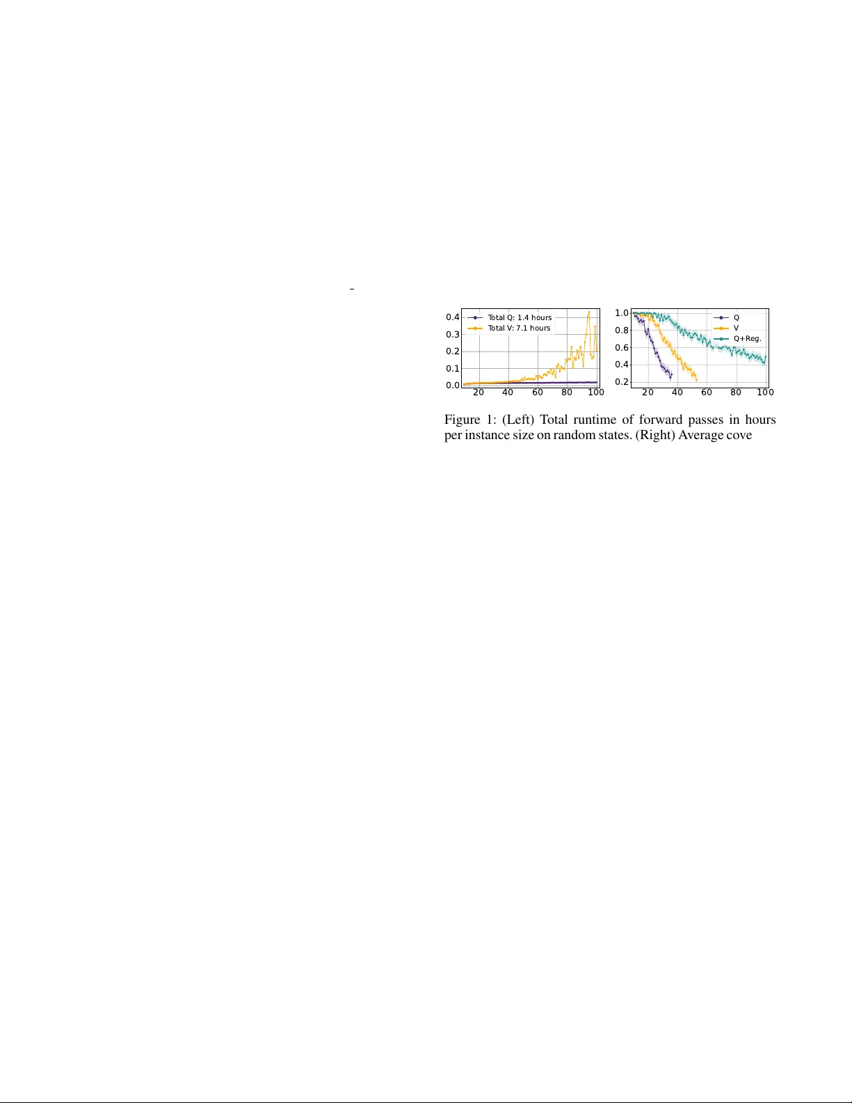
P er -Domain Generalizing P olicies: On Learning Efficient and Rob ust Q-V alue Functions (Extended V ersion with T echnical A ppendix) Nicola J. M ¨ uller 1,2,3 , Moritz Oster 1,2 , Isabel V alera 2 , J ¨ org Hoffmann 1,2 , Timo P . Gros 1,2,3 1 German Research Center for Artificial Intelligence (DFKI), Saarbr ¨ ucken, Germany 2 Saarland Univ ersity , Saarland Informatics Campus, Saarbr ¨ ucken, Germany 3 Center for European Research in T rusted Artificial Intelligence (CER T AIN) { Nicola.Mueller , Moritz.Oster , Timo Phillip.Gros } @dfki.de, { iv alera,hof fmann } @cs.uni-saarland.de Abstract Learning per-domain generalizing policies is a ke y challenge in learning for planning. Standard approaches learn state- value functions represented as graph neural networks using supervised learning on optimal plans generated by a teacher planner . In this w ork, we adv ocate for learning Q-value func- tions instead. Such policies are drastically cheaper to e v aluate for a giv en state, as they need to process only the current state rather than every successor . Surprisingly , v anilla supervised learning of Q-v alues performs poorly as it does not learn to distinguish between the actions taken and those not taken by the teacher . W e address this by using regularization terms that enforce this distinction, resulting in Q-value policies that con- sistently outperform state-value policies across a range of 10 domains and are competitiv e with the planner LAMA-first. Code — https://doi.org/10.5281/zenodo.19069966 1 Introduction Learning per -domain generalizing policies using neural net- works is g aining popularity in planning (T oyer et al. 2020; St ˚ ahlberg, Bonet, and Geffner 2022a,b, 2025; Rossetti et al. 2024; W ang and Thi ´ ebaux 2024; Chen et al. 2025a,b). The key challenge is to foster scaling behavior , i.e., generalizing from small training instances to large test instances. Prior work used graph neural networks (GNNs) to learn state-value functions V : S → R + for classical plan- ning domains, which approximate the optimal heuristic h ∗ (St ˚ ahlberg, Bonet, and Geffner 2022a,b, 2025; Gros et al. 2025). Given V , a per-domain generalizing policy is com- puted as π ( s ) = arg min a cost( a ) + V ( s ′ ) , where s ′ is the respectiv e successor reached through action a . Observe that choosing an action this way requires the GNN to process e very successor state. This can be very in- effecti v e and impede scaling performance, e v en when using batch processing. This motiv ates learning a Q-value function Q : S × Act → R + instead, which approximates the cost of an optimal plan starting with a giv en action a from a giv en state s (Sutton, Barto et al. 1998). A policy can then be com- puted as π ( s ) = arg min a Q ( s, a ) , which only requires the current state to compute the Q-values of all applicable ac- tions with a single GNN forward pass. Figure 1 (left) sho ws the runtime per instance size on random states for the IPC’23 20 40 60 80 100 0.0 0.1 0.2 0.3 0.4 T otal Q: 1.4 hours T otal V : 7.1 hours 20 40 60 80 100 0.2 0.4 0.6 0.8 1.0 Q V Q+R eg. Figure 1: (Left) T otal runtime of forward passes in hours per instance size on random states. (Right) A verage coverage and confidence interv al per instance size for trained policies. domain Rovers (T aitler et al. 2024), where a Q-v alue policy is 5 times faster than a state-v alue policy . W e lev erage existing planners to train our Q-value func- tions using supervised learning (SL), where the training data consist of optimal plans (St ˚ ahlberg, Bonet, and Gef fner 2022a; Rossetti et al. 2024; Gros et al. 2025). T o the best of our knowledge, this has not been tried before for learn- ing per -domain generalizing policies. Surprisingly , we sho w that the vanilla use of SL for Q-values yields policies that generalize poorly , despite fitting the training data well. Con- sider Figure 1 (right), which sho ws the av erage coverage per instance size of state (orange) vs. Q-value (purple) policies. Both policies were trained on the same optimal plans using the same loss; yet, the state-v alue policy generalizes much better than the Q-value policy . This is because the Q-values are often identical for all actions, leading to random action selection. In other words, the Q-v alues fail to distinguish be- tween the actions taken and not taken by the teacher planner . Our k ey contribution is sho wing that this can be fix ed. W e extend the SL objectiv e with a regularization term that en- forces the Q-values of non-teacher actions to be larger than those of teacher actions. This approach is shown in green in Figure 1 (right), and it vastly outperforms the state-value policy . Importantly , this difference is strictly due to better action selection, as policy runs are only limited by the num- ber of actions, without any runtime limit. W e ev aluate our approach with three GNN architectures on 10 domains and find that the trends from Figure 1 (right) apply consistently , yielding regularized Q-value policies that outperform state-v alue policies and are competiti v e with the planner LAMA-first. 2 Efficiency of State and Q-V alue Policies Here, we show that Q-value policies are more ef ficient than state-v alue policies using three graph neural network (GNN) architectures for per-domain generalizing policies. GNN architectur es. The r elational gr aph neural network (R-GNN) is a specialized GNN architecture that operates di- rectly on the relational structure induced by classical plan- ning states, maintaining embeddings of a state’ s objects and passing information between them according to the ground atoms of which they are arguments (St ˚ ahlberg, Bonet, and Geffner 2022a). Con versely , the object encoding (OE) and object-atom encoding (O AE) define graph representations of states that can be processed by of f-the-shelf GNN archi- tectures (Hor ˇ c ´ ık and ˇ S ´ ır 2024); we use the r elational graph con volutional network (RGCN) (Schlichtkrull et al. 2018), as in prior work (Chen, Thi ´ ebaux, and T re vizan 2024). In a nutshell, OE defines nodes for a state’ s objects and adds edges between objects occurring in the same ground atoms, whereas OAE defines nodes for both objects and atoms, adding edges between atoms and their arguments. All three GNN architectures have in common that they iterativ ely compute embeddings for ev ery object in a giv en state. Independent of the architecture, the object embeddings can be aggregated into a state embedding, which is then used to predict either a single state-value or the Q-v alues of all applicable actions. W e use the approach of St ˚ ahlberg and Geffner (2025). For the sake of brevity , we omit the details here and provide a description in the technical appendix B. Policy efficiency . T o compute a policy using state-v alues, i.e., π ( s ) = arg min a cost( a ) + V ( s ′ ) , we need to pre- dict the values of all successor states s ′ . This requires ex- panding the current state, translating the successors into GNN input, combining them into a single batch, and pass- ing it to the GNN. T o compute a policy using Q-v alues, i.e., π ( s ) = arg min a Q ( s, a ) , we need to predict the values of all applicable actions in the current state s . This only re- quires translating the current state into GNN input and pass- ing it to the GNN. Hence, state-value policies are less ef- ficient than Q-value policies because they require process- ing every successor of the current state instead of the cur- rent state only . When scaling the instance size, the ov erhead for computing state-v alues gro ws drastically , as a lar ger in- stance size typically coincides with a larger branching factor , and, thus, more successors to process at ev ery state. Consider T able 1, which compares the runtimes of state and Q-v alue policies on the 10 domains used in Section 4. For each domain, we generate a set of states using random walks of length 25 for 25 instances per size, ranging from the smallest possible instance size up to 100 . For each state, we predict an action using a randomly initialized state or Q-value polic y and record the total runtime. All policies are ex ecuted on an NVIDIA R TX A 6000 GPU. Across all archi- tectures, we see that the a verage runtimes of the state-v alue policies are between 4 and 18 times higher than those of the Q-value policies. W e conclude that Q-values should be preferred over state-values for per-domain generalizing poli- cies, as they scale much more ef ficiently with instance size. R-GNN OE O AE Domain V Q V Q V Q Blocksworld 0.6 0.5 1.8 2.0 0.7 0.4 Childsnack 7.2 0.9 21.7 4.3 28.6 0.7 Ferry 0.8 0.5 2.5 2.0 1.6 0.4 Floortile 1.9 1.0 7.9 4.0 4.0 0.6 Gripper 1.0 0.6 3.1 2.2 1.9 0.5 Logistics 2.7 0.7 7.3 2.3 10.2 0.6 Rov ers 7.1 1.4 39.8 7.5 25.4 1.1 Satellite 4.6 0.8 14.7 3.5 16.0 0.7 T ransport 6.5 0.7 22.8 2.7 18.0 0.7 V isitall 0.4 0.2 1.1 0.6 0.9 0.3 A verage 3.3 0.7 12.3 3.1 10.7 0.6 T able 1: T otal runtime in hours for randomly initialized state and Q-value policies on sets of random states. 3 Regularization T erms for Super vised Learning of Q-V alue Functions W e no w show why vanilla supervised learning (SL) fails to learn Q-v alue functions for per-domain generalizing poli- cies, and then fix this by introducing regularization terms. 3.1 Supervised Lear ning of Q-V alue Functions Prior work learned state-v alue functions using SL, where the training data consist of optimal plans for small domain in- stances (St ˚ ahlberg, Bonet, and Geffner 2022a; Gros et al. 2025). Ho we ver , we find that learning Q-v alue functions us- ing this approach yields policies that fail to generalize. This is because the Q-v alue functions tend to predict the same Q- values for all actions applicable in a given state, leading to random action selection. W e in vestigate this behavior by comparing Q-v alue func- tions successfully learned for 10 domains using the R-GNN, OE, and O AE architectures. W e refer to Section 4 for train- ing details. For each model, we compute the average predic- tion error for the Q-values of teacher actions a ∗ in the train- ing set ( Err ), i.e., | h ∗ ( s ) − Q ( s, a ∗ ) | . W e also compute the av erage difference in predicted Q-values between teacher actions a ∗ and non-teacher actions a i ∈ Act ( s ) \{ a ∗ } in the training set ( Diff ), i.e., | Q ( s, a ∗ ) − Q ( s, a i ) | . W e present the av erages of both scores over 10 domains. Consider the left column ( Q ) in T able 2. All models fit their training data well, as the av erage prediction errors for teacher actions ( Err ) are small, with v alues between 0 . 54 and 2 . 15 . Howe ver , the models tend to predict the same Q-v alues for teacher and non-teacher actions, as the av erage Q-v alue differences ( Diff ) are between 0 . 71 and 0 . 96 . Hence, Q-value policies learned using v anilla SL perform poorly because they fail to generalize to non-teacher actions. 3.2 Regularizing Q-V alue Functions T o ensure that learned Q-v alue functions distinguish be- tween teacher and non-teacher actions, we extend the SL objectiv e with a regularization term. The extended learning objectiv e is defined as θ ∗ = arg min θ E ( s,a ∗ ) ∼ D [ L ( s, a ∗ ) + λ · Ω( s, a ∗ )] , where θ ∗ are the parameters of the Q-v alue function Q that minimizes the loss L subject to the regularizer Ω , and λ Q Ω Exp. Ω Heu. R-GNN OE O AE R-GNN OE O AE R-GNN OE O AE Err Diff Err Diff Err Diff Err Diff Err Diff Err Diff Err Diff Err Diff Err Diff A verage 0.54 0.71 1.37 0.96 2.15 0.84 0.70 4.69 0.70 7.66 0.91 6.66 0.73 97.55 1.25 46.25 0.83 152.52 T able 2: Prediction errors for teacher actions ( Err ), and Q-v alue differences between teacher and non-teacher actions ( Diff ). is the regularization coefficient. The role of L is to ensure that Q predicts the Q-values of teacher actions a ∗ accu- rately , whereas Ω ensures that the Q-values of non-teacher actions a i are larger than those of teacher actions a ∗ , i.e., ∀ a i ∈ Act ( s ) \{ a ∗ } : Q ( s, a i ) > Q ( s, a ∗ ) . W e define the regularization term in general as Ω( s, a ∗ ) = X a i ∈ Act ( s ) \{ a ∗ } max { 0 , B − Q ( s, a i ) } , where B is a lo wer bound for the Q-values of non-teacher actions a i . The penalty induced by Ω increases linearly if Q ( s, a i ) is smaller than B , whereas there is no penalty if Q ( s, a i ) ≥ B holds. W e now introduce two regularizers Ω that differ in ho w the y compute the lo wer bound B . Explicit regularizer . The explicit re gularizer Ω Exp. com- putes B using the h ∗ values of the states s in the training data, which is feasible as they are on optimal trajectories. W e define the lo wer bound as B Exp. ( s ) = h ∗ ( s ) + 1 , ensuring that the Q-values of non-teacher actions Q ( s, a i ) are strictly larger than the target values of teacher actions Q ( s, a ∗ ) = h ∗ ( s ) . While this biases learning tow ards an inadmissible Q-value function, as there might be multiple optimal actions, we can still conv erge to an optimal policy since teacher actions always have the lowest Q-values. W e note that, in general, admissibility cannot be guaranteed for a learned Q-value function, e v en without this bias. Heuristic regularizer . The heuristic re gularizer Ω Heu. uses an admissible heuristic to compute action-dependent lower bounds B i , which provide more information about the true Q-v alues of non-teacher actions a i . First, we compute a lower bound cost( a i ) + h ( s ′ i ) for every a i , where s ′ i is the successor reached through action a i , and h is an admissi- ble heuristic; in this paper, h LMcut (Helmert and Domshlak 2009) 1 . Howe ver , this lo wer bound may not be strictly larger than the target Q-value of the teacher action, i.e., h ∗ ( s ) , prev enting us from distinguishing between non-teacher and teacher actions. Thus, we compute the final lower bound as B Heu. ( s, a i ) = max { h ∗ ( s ) + 1 , cost( a i ) + h ( s ′ i ) } . On a verage, B Heu. is tighter than B Exp. for 17% of the non- teacher actions in the training sets used in Section 4. Comparing regularizers. Consider again T able 2, where the middle ( Ω Exp. ) and right ( Ω Heu. ) columns show the pre- diction errors ( Err ) and Q-value differences ( Diff ) for Q- value functions trained using the explicit and heuristic reg- ularizers, respectiv ely . Compared to vanilla SL on the left 1 For dead-ends, i.e., h LMcut ( s ′ i ) = ∞ , we use a v alue of 1120 , which is drastically larger than all plans in our training data. ( Q ), the Q-value differences increase while the prediction errors mostly decrease, suggesting that the regularizers not only help to distinguish between non-teacher and teacher ac- tions but can also help to predict the Q-values of teacher actions more accurately . The Ω Heu. models also have con- siderably larger Q-value differences than the Ω Exp. models, which is due to the high predicted v alue for actions leading to dead-ends. 4 Experiments In this section, we outline our data set construction and train- ing setup, and then e v aluate our approaches with respect to scaling behavior and IPC test set performance. Data sets. W e consider the domains from the IPC’23 learning track (T aitler et al. 2024), where we omit Miconic and Spanner because all policies immediately achie v e 100% cov erage, and Sokoban because its generator requires unfea- sibly many runs until a solvable instance is generated. W e also consider the Gripper, Logistics, and V isitall domains from the FF domain collection 2 . T o construct training sets for each domain, we use the publicly av ailable generators to uniformly sample up to 100 unique instances per size, ranging from size 2 to 100 . W e use the seq-opt-merge-and-shrink configuration of Fast Down- ward (Helmert 2006) with limits of 20 minutes and 64 GB as the optimal teacher planner, deleting instances that were not solved. W e provide full details about the training sets in the technical appendix C. For validation, we use Gros et al.’ s dynamic co verage validation, which does not require a pre- computed validation set, as it runs policies on increasingly large instances generated on-the-fly (2025). T raining setup. W e train state, Q, and regularized Q-value functions using the R-GNN, OE, and O AE architectures. As the loss function L , we use the mean absolute err or ( MAE ), which is defined as MAE( s ) = | h ∗ ( s ) − V ( s ) | for state-values and as MAE( s, a ∗ ) = | h ∗ ( s ) − Q ( s, a ∗ ) | for Q-v alues. In preliminary experiments, we also tested the mean squared error and temporal difference error losses, but found that MAE yields the best policies. For the regular- ized Q-value functions, we use a regularization coefficient of λ = 1 . 0 , gi ving equal weight to L and Ω . W e repeat the training using three random seeds and return the pol- icy with the best validation performance. When running the policies, we forbid revisiting states to prev ent cycles, as in prior work (St ˚ ahlberg, Bonet, and Gef fner 2022a,b, 2023). Scaling beha vior evaluation. W e use Gros et al.’ s scaling behavior ev aluation to compare how well the trained policies 2 https://fai.cs.uni- saarland.de/hof fmann/f f- domains.html R-GNN OE OAE V Q Ω Exp. Ω Heu. V Q Ω Exp. Ω Heu. V Q Ω Exp. Ω Heu. Domain Scale SCov Scale SCov Scale SCov Scale SCov Scale SCov Scale SCov Scale SCov Scale SCov Scale SCov Scale SCov Scale SCov Scale SCov Blocksworld 52 44.5 5 1.6 54 47.8 55 48.2 14 9.2 5 1.2 48 40.5 50 42.4 37 27.5 4 1.3 52 44.9 52 44.6 Childsnack 71 43.4 16 4.2 100 93.0 100 93.0 26 12.0 9 0.2 82 43.1 98 46.9 31 15.9 36 14.9 100 65.8 83 41.5 Ferry 100 84.5 30 12.9 100 85.2 100 84.5 33 19.8 21 10.9 100 80.2 100 80.1 45 26.4 7 2.1 100 79.5 100 80.1 Floortile 8 0 8 0 60 44.5 62 45.6 8 0 8 0 50 28.8 56 43.2 8 0 8 0 59 42.0 62 45.9 Rovers 53 29.8 36 17.1 100 66.5 100 64.4 25 9.8 33 13.3 48 24.6 46 23.0 22 8.3 28 9.8 60 30.1 61 29.8 Satellite 50 28.2 37 21.5 100 69.4 100 69.1 20 9.8 25 12.9 73 45.3 73 45.2 24 9.7 6 0.2 92 55.1 90 55.5 Transport 72 46.6 46 24.7 100 90.4 100 92.7 38 20.1 42 23.1 100 88.6 100 89.7 19 9.3 57 32.1 100 89.7 100 89.6 Gripper 100 77.5 36 15.2 100 88.8 100 88.9 100 83.0 63 33.4 100 88.9 100 88.4 100 88.6 100 73.8 100 88.5 100 88.6 Logistics 47 24.9 50 25.9 100 82.4 100 84.3 36 19.8 52 27.0 100 86.2 100 85.7 38 22.6 57 31.2 100 77.0 100 75.6 V isitall 256 11.4 256 11.4 961 25.1 961 22.8 196 9.5 144 5.7 961 22.7 961 22.1 529 13.4 484 14.9 961 24.8 676 16.6 T able 3: Scale and SCov scores of the scaling behavior ev aluation. Bold scores are the best for each architecture, and highlighted scores are the best ov erall. R-GNN V Ω Exp. Ω Heu. LAMA-first Domain Cov Len Cov Len Cov Len Cov Len Blocksworld 47.8 90.0 78.9 233.1 78.9 232.1 56.7 288.7 Childsnack 5.6 41.2 51.1 41.4 54.4 41.5 35.2 41.8 Ferry 54.4 73.7 67.8 119.6 67.8 119.6 67.8 150.3 Floortile 0.0 — 36.7 93.5 37.8 109.3 16.9 51.0 Rovers 24.4 49.0 36.7 66.2 37.8 80.3 57.8 171.0 Satellite 32.2 36.9 64.4 71.2 66.7 68.2 85.6 104.4 T ransport 24.4 69.6 70.0 91.3 74.4 96.8 64.4 70.7 A verage 27.0 60.1 57.9 102.3 59.7 106.8 54.9 125.4 T able 4: Coverage in percent (Cov) and av erage plan length (Len) on IPC’23 test sets. Bold scores are the best cov erages for each domain. generalize (2025). F or a given instance size n , the ev aluation runs a policy on uniformly generated instances until the es- timate of the a verage coverage ˆ C n for size n is within a 10% confidence interval with 90% probability . This process re- peats with an increasing size n until the cov erage ˆ C n drops below 30% or the maximum size of 100 ( 1000 for V isitall) is reached. Policy runs hav e a step limit of 100 + n that in- creases with the instance size n . The ev aluation results are reported using two summary scores: Scale is the largest in- stance size n before termination, which measures how far the polic y generalizes, and SCov is the sum of co verages ˆ C n per size n , which measures ov erall performance. T able 3 sho ws the summary scores for the scaling be- havior ev aluation of all policies. W e observe the follow- ing trends across all architectures: The v anilla Q-v alue poli- cies ( Q ) perform the worst overall. This is due to failing to distinguish teacher and non-teacher actions, as sho wn in Section 3. Importantly , we see that the state-value poli- cies ( V ) are consistently outperformed by the regularized Q- value policies ( Ω Exp. & Ω Heu. ). This shows that the additional learning signals provided by regularizing the Q-values of non-teacher actions lead to vastly improv ed generalization. Lastly , we see that the policies trained using the heuristic regularizer ( Ω Heu. ) outperform the explicit regularizer poli- cies ( Ω Exp. ) on some domains. This sho ws that providing tighter lo wer bounds for the Q-v alues of non-teacher actions can further improv e generalization. IPC test sets. W e additionally ev aluate our policies on the IPC’23 test sets, which provides insights into their perfor- mance on particularly dif ficult instances. W e consider only the R-GNN architecture, as it showed the overall best per- formance in the scaling behavior ev aluation, and we omit the vanilla Q-value policies due to their poor performance. W e ensured that the training and test sets do not ov erlap. All policies are e xecuted on an AMD EPYC 9454 CPU with time and memory limits of 1 minute and 8 GB. As a base- line, we run the LAMA-first planner (Richter and W estphal 2010) using the same hardware and limits. Consider T able 4, which shows the co verage and average plan length for the 7 considered IPC’23 domains. As be- fore, our regularized Q-value policies consistently achiev e higher cov erages than the state-v alue policies. Impressi vely , the coverages and plan lengths of the regularized Q-value policies are competitiv e with those of LAMA-first. 5 Conclusion Learning per-domain generalizing policies is becoming in- creasingly popular , and supervised learning pro vides a natu- ral training framework as we can lev erage optimal planners to generate rich training data. In this work, we have sho wn that the common approach of learning state-value functions yields policies whose runtime scales poorly with instance size. The more efficient approach of learning Q-value func- tions, howe v er , f ails to learn the distinction between teacher and non-teacher actions. Hence, we introduce regularization terms that use optimal and admissible heuristics to enforce the Q-values of non-teacher actions to be larger than those of teacher actions. Experiments on 10 domains using three GNN architectures show that our regularized Q-value poli- cies are not only more efficient but also achieve vastly higher generalization than state-value policies. A promising ne xt step for our work would be to continue the policy training using reinforcement learning on dynam- ically generated instances. These instances could be gener- ated as needed, e.g., we could gradually increase their size to improve scaling or focus on instances where the policy previously f ailed. Acknowledgements This work was partially supported by the German Federal Ministry of Education and Research (BMBF) as part of the project MA C-MERLin (Grant Agreement No. 01IW24007), by the German Research Foundation (DFG) - GRK 2853/1 “Neuroexplicit Models of Language, V ision, and Action” - project number 471607914, and by the European Regional Dev elopment Fund (ERDF) and the Saarland within the scope of (T o)CER T AIN. References Chen, D. Z.; Hao, M.; Thi ´ ebaux, S.; and T revizan, F . 2025a. Graph Learning for Planning: The Story Thus Far and Open Challenges. In AAAI W orkshop on Gener alization in Plan- ning . Chen, D. Z.; Thi ´ ebaux, S.; and Tre vizan, F . 2024. Learning Domain-Independent Heuristics for Grounded and Lifted Planning. In Pr oceedings of the AAAI Confer ence on Ar- tificial Intelligence , v olume 38, 20078–20086. Chen, D. Z.; Zenn, J.; Cinquin, T .; and McIlraith, S. A. 2025b. Language models for PDDL planning: Generating sound and programmatic policies. In Eighteenth Eur opean W orkshop on Reinfor cement Learning . Ghallab, M.; Nau, D.; and Tra verso, P . 2004. Automated Planning: theory and practice . Elsevier . Gros, T . P .; M ¨ uller , N. J.; Fi ˇ ser , D.; V alera, I.; W olf, V .; and Hoffmann, J. 2025. Per-domain generalizing policies: On validation instances and scaling behavior . In Pr oceedings of the International Confer ence on Automated Planning and Scheduling , v olume 35, 198–203. Helmert, M. 2006. The fast downw ard planning system. Journal of Artificial Intellig ence Resear c h , 26: 191–246. Helmert, M.; and Domshlak, C. 2009. Landmarks, critical paths and abstractions: what’ s the difference anyway? In Pr oceedings of the International Conference on Automated Planning and Scheduling , v olume 19, 162–169. Hor ˇ c ´ ık, R.; and ˇ S ´ ır , G. 2024. Expressi v eness of graph neural networks in planning domains. In Pr oceedings of the Inter- national Conference on Automated Planning and Schedul- ing , volume 34, 281–289. Hor ˇ cik, R.; ˇ S ´ ır , G.; ˇ Simek, V .; and Pevn ` y, T . 2025. State En- codings for GNN-Based Lifted Planners. In Pr oceedings of the AAAI Conference on Artificial Intelligence , volume 39, 26525–26533. Kingma, D. P . 2014. Adam: A method for stochastic opti- mization. arXiv pr eprint arXiv:1412.6980 . Misra, D. 2020. Mish: A Self Regularized Non-Monotonic Activ ation Function. In Proceedings of the British Machine V ision Confer ence 2020 . British Machine V ision Associa- tion. Richter , S.; and W estphal, M. 2010. The LAMA planner: Guiding cost-based anytime planning with landmarks. Jour- nal of Artificial Intelligence Resear c h , 39: 127–177. Rossetti, N.; T ummolo, M.; Gere vini, A. E.; Putelli, L.; Se- rina, I.; Chiari, M.; and Oliv ato, M. 2024. Learning General Policies for Planning through GPT Models. In Pr oceedings of the International Confer ence on Automated Planning and Scheduling , v olume 34, 500–508. Schlichtkrull, M.; Kipf, T . N.; Bloem, P .; V an Den Ber g, R.; T itov , I.; and W elling, M. 2018. Modeling relational data with graph con volutional networks. In Eur opean semantic web confer ence , 593–607. St ˚ ahlberg, S.; Bonet, B.; and Geffner , H. 2022a. Learning general optimal policies with graph neural networks: Ex- pressiv e power , transparency , and limits. In Pr oceedings of the International Confer ence on Automated Planning and Scheduling , v olume 32, 629–637. St ˚ ahlberg, S.; Bonet, B.; and Geffner , H. 2022b. Learning Generalized Policies without Supervision Using GNNs. In Pr oceedings of the International Conference on Principles of Knowledge Repr esentation and Reasoning , 474–483. St ˚ ahlberg, S.; Bonet, B.; and Geffner , H. 2023. Learning general policies with policy gradient methods. In Pr oceed- ings of the International Conference on Principles of Knowl- edge Repr esentation and Reasoning , 647–657. St ˚ ahlberg, S.; Bonet, B.; and Geffner , H. 2025. Learning More Expressive General Policies for Classical Planning Domains. In Proceedings of the AAAI Conference on Ar- tificial Intelligence , v olume 39, 26697–26706. St ˚ ahlberg, S.; and Gef fner , H. 2025. First-Order Rep- resentation Languages for Goal-Conditioned RL. CoRR , abs/2512.19355. Sutton, R. S.; Barto, A. G.; et al. 1998. Reinfor cement learn- ing: An intr oduction , v olume 1. MIT press Cambridge. T aitler , A.; Alford, R.; Espasa, J.; Behnke, G.; Fi ˇ ser , D.; Gimelfarb, M.; Pommerening, F .; Sanner , S.; Scala, E.; Schreiber , D.; et al. 2024. The 2023 International Planning Competition. AI Magazine , 45(2): 280–296. T oyer , S.; Thi ´ ebaux, S.; Tre vizan, F . W .; and Xie, L. 2020. ASNets: Deep Learning for Generalised Planning. Journal of Artificial Intelligence Resear c h , 68: 1–68. W ang, R. X.; and Thi ´ ebaux, S. 2024. Learning generalised policies for numeric planning. In Pr oceedings of the Interna- tional Conference on Automated Planning and Scheduling , volume 34, 633–642. A Classical Planning A classical planning problem can be represented as a pair ⟨ D , I ⟩ , consisting of a domain D and an instance I (Ghal- lab, Nau, and T rav erso 2004). The domain D defines a set of predicates P ∈ P and a set of action schemas A ∈ A , each of which describes arguments, preconditions, effects, and action costs. The instance I defines a set of objects o ∈ O , using which we can deriv e ground atoms p := P ( o 0 , . . . , o n ) and ground actions a := A ( o 0 , . . . , o n ) . Fur- ther , I defines an initial state I nit and a set of goal condi- tions G , both of which are sets of ground atoms. T ogether , D and I encode a state model ⟨S , s 0 , S G , Act, f ⟩ , consist- ing of a set of states s ∈ S , the initial state s 0 , the set of goal states S G , the sets of applicable ground actions for each state Act ( s ) , and the transition function f : S × Act → S . A plan is a sequence of ground actions  a = ⟨ a 0 , . . . , a T − 1 ⟩ that transitions from the initial state s 0 to any goal state s T ∈ S G . A plan  a ∗ is optimal if the sum of the costs of its actions is minimal. The optimal heuristic value h ∗ ( s ) of a state s is defined as the cost of an optimal plan starting in state s . B Graph Neural Networks f or P er -Domain Generalizing Policies Computing a per -domain generalizing policy requires a neu- ral network architecture that handles variable-sized inputs because the number of ground atoms that can be true in any giv en state increases with the instance size. Graph neural networks (GNNs) are one such architecture, and they have become a standard choice for learning per-domain general- izing policies because classical planning states can be ef fec- tiv ely represented as graphs (St ˚ ahlberg, Bonet, and Geffner 2022a; Chen, Thi ´ ebaux, and T re vizan 2024; Chen et al. 2025a; Hor ˇ cik et al. 2025). Graph Neural Networks. Gi ven a graph G = ⟨V , E ⟩ with nodes V and edges E , a GNN computes for e very node v ∈ V an embedding h v . Each embedding h l v is iterativ ely com- puted over L GNN layers l , where the initial embedding h 0 v corresponds to the node’ s feature vector as specified by G . The computation of each layer can be divided into two steps: 1. A G G R E G A T E : The embeddings h l u of all nodes u in the neighborhood N ( v ) , i.e., ∀ u ∈ V : ⟨ u, v ⟩ ∈ E , are ag- gregated. 2. C O M B I N E : The aggregated embeddings h l u and the node’ s current embedding h l v are combined to compute the updated embedding h l +1 v . These steps can be expressed as the general update rule h l +1 v = C O M B I N E ( h l v , A G G R E G AT E ( { { h l u | u ∈ N ( v ) } } )) , (1) where { { . . . } } denotes a multiset. The update is applied to each node v ∈ V simultaneously and for each layer l itera- tiv ely until we obtain the final node embeddings h L v . T o demonstrate the generality of our findings and meth- ods, we consider three dif ferent GNN architectures for learn- ing per-domain generalizing policies. Object & object-atom encodings. The object encoding (OE) and object-atom encoding (O AE) define graph repre- sentations of classical planning states that can be processed by off-the-shelf GNN architectures (Hor ˇ c ´ ık and ˇ S ´ ır 2024; Hor ˇ cik et al. 2025). The key difference between these encod- ings is that OE defines nodes for a state’ s objects, whereas O AE defines nodes for objects and ground atoms. T o encode information about the goal conditions G , we introduce a goal version P G of each predicate P ∈ P and extend ev ery state s ∈ S with the corresponding ground atoms P G ( o 0 , . . . , o n ) ∈ G . Further, we assign a unique identifier i ∈ N to e very predicate P i ∈ P . Lastly , we treat nullary atoms as unary atoms that hold for all objects, i.e., ∀ o ∈ O : P i ( o ) ∈ s . Definition 1 (Object Encoding) . F or a gi v en state s , OE de- fines its graph representation as G = ⟨V , E , f , l ⟩ , where • V = O • E = {⟨ o u , o w ⟩ P i | P i ( . . . , o u , . . . , o w , . . . ) ∈ s } • f : V → { 0 , 1 } m , with f ( o ) i = 1 [ P i ( o ) ∈ s ] • l : E → N , with l ( ⟨ o u , o w ⟩ P i ) = i . In other words, we hav e a node for ev ery object o with a node feature f ( o ) that is a multi-hot encoding of the unary predicates P i for which there is an atom P i ( o ) ∈ s . Fur- ther , if two objects o u and o w are arguments of an atom P i ( . . . , o u , . . . , o w , . . . ) ∈ s , we have an undirected edge ⟨ o u , o w ⟩ P i with a label l ( ⟨ o u , o w ⟩ P i ) corresponding to the predicate’ s identifier i . Definition 2 (Object-Atom Encoding) . For a giv en state s , O AE defines its graph representation as G = ⟨V , E , f , l ⟩ , where • V = O ∪ s • E = {⟨ o u , p ⟩ | p := P i ( . . . , o u , . . . ) ∈ s } • f : V → { 0 , 1 } m , with f ( o ) i = 1 [ P i ( o ) ∈ s ] and f ( p ) i = 1 [ p = P i ( . . . )] • l : E → N , with l ( ⟨ o u , p ⟩ ) = u . In other words, we have a node for e very object o and ground atom p , where objects’ node features f ( o ) are multi-hot en- codings of the unary atoms P i ( o ) ∈ s , and atoms’ node fea- tures f ( p ) are one-hot encodings of their predicate P i . W e connect atoms p to their arguments o u via undirected edges ⟨ o u , p ⟩ , which are labeled by the argument’ s position u . W e process the OE and O AE graphs using the r elational graph con volutional network (RGCN) (Schlichtkrull et al. 2018) architecture with the embedding update rule h l +1 v = σ W l h l v + X r ∈ R max u ∈N r ( v ) W l r h l u ! , where N r ( v ) is the set of all nodes u connected to node v via an edge with the label r ∈ R , and W l r is a label-specific weight matrix. Each layer is followed by a Mish activ ation function (Misra 2020). Relational graph neural network. The r elational graph neural network (R-GNN) is a specialized GNN architecture that operates directly on the relational structure of states in- stead of translating them into graphs (St ˚ ahlberg, Bonet, and Geffner 2022a). Like OE and O AE, the R-GNN also in- troduces goal predicates P G to encode goal conditions into states. Algorithm 1: Relational graph neural network. Input: Set of atoms p ∈ s and objects o ∈ s Output: Object embeddings h L o 1 h 0 o ← 0 k for each object o ∈ s ; 2 for l = 1 , . . . , L do 3 for each atom p := P ( o 1 , ..., o n ) ∈ s do 4 m p,o u ←  MLP P ( h l o 1 , ..., h l o n )  u ; 5 for each object o do 6 m o ← aggregate ( { { m p,o | o ∈ p } } ) ; 7 h l +1 o ← h l o + MLP U ( h l o , m o ) ; Consider Algorithm 1, which sho ws a forward pass of the R-GNN. The object embeddings h 0 o initially contain only ze- ros. The R-GNN then updates them over L layers, each con- sisting of two steps: 1. Message Computation (lines 3-4): For each atom p := P ( o 1 , ..., o n ) ∈ s , we pass the inv olved objects’ embed- dings h l o to a predicate-specific MLP P , which computes a message m p,o for each argument o of p . 2. Embedding Update (lines 5-7): F or each object o , we ag- gregate the messages m p,o into a single message m o by applying a dimension-wise smooth maximum. The up- dated embedding h l +1 o is then computed by passing h l o and m o to MLP U , with the addition of a residual connec- tion. Computing state or Q-values. All three GNN architec- tures have in common that they iterativ ely compute embed- dings for e very object in a given state. Independent of the architecture, these embeddings can then be used to predict either a single state-v alue or a Q-value for e very applica- ble action. W e here follow the approach of St ˚ ahlberg and Geffner (2025). First, we compute a dimension-wise sum o ver the (node) embeddings of all objects to obtain a single state embedding h s = X o ∈O h L o . T o compute a state-value, we simply pass the state embed- ding to a final MLP V ( s ) = MLP ( h s ) . T o compute Q-values, howe ver , we need to encode the ap- plicable actions a ∈ Act ( s ) into each state s . Accordingly , we introduce a predicate P A for each action scheme A ∈ A and action objects o a for all ground actions a ∈ Act ( s ) . W e then extend each state with ne w ground atoms p := P A ( o a , o 0 , . . . , o n ) . The R-GNN, OE, and OAE architec- tures then process the extended state encodings as they did before. Finally , we compute the Q-values by concatenating each ground action embedding with a copy of the state em- bedding and passing it to an MLP Q ( s, a ) = MLP ( h L a ∥ h s ) . C T raining Details W e here provide additional details about our training setup. Hyperparameters. Each polic y is trained using three ran- dom seeds, where each training run consists of up to 100 epochs with a batch size of 256 . Policy updates are com- puted using the Adam optimizer (Kingma 2014) with a learning rate of 0 . 0002 for the state-value and vanilla Q- value models, and a higher learning rate of 0 . 002 for the regularized Q-v alue models, since we found them to be less prone to overfitting. W e additionally limit the magnitude of each policy update using gradient clipping with a value of 0 . 1 . F or the R-GNN architecture, we use a hidden size of 32 and 30 layers with shared parameters. For the RGCN archi- tecture, which processes the OE and O AE graphs, we use a hidden size of 32 and 30 layers with separate parameters. Data sets. For a gi ven domain, we check for each size n ∈ [2 , . . . , 100] whether it is possible to generate a cor- responding instance. If so, we uniformly sample generator inputs that yield an instance of size n and pass them to the generator . The generators were either taken from the IPC’23 (T aitler et al. 2024) or from the FF domain collec- tion 3 . If the generator returns an instance that has already been generated or where the initial state already satisfies the goal, we discard it. After generating all instances, we pass each to the seq-opt-mer ge-and-shrink configuration of Fast Do wn- ward (Helmert 2006) with limits of 20 minutes and 64 GB, and delete every instance for which no opti- mal plan was found. T able 5 shows the sizes of the solved instances. Then, for each optimal plan, we compute the h LMcut (Helmert and Domshlak 2009) values of the siblings of each state along the optimal trajectory . The final data sets then consist of tuples  s, h ∗ ( s ) , a ∗ , a 1 , . . . , a m , h LMcut ( s ′ 1 ) , . . . , h LMcut ( s ′ m )  , where s is a state on the optimal trajectory , h ∗ ( s ) is its optimal heuristic value, a ∗ is the teacher action, a i are the non-teacher actions, and h LMcut ( s ′ i ) are the heuristic v alues of the successors s ′ i reached through a i . Domain T raining Set Sizes Blocksworld [2 − 16] Childsnack [8 − 38] Ferry [3 − 25] Floortile [7 − 18] Rov ers [10 − 26] Satellite [5 − 31] T ransport [6 − 38] Gripper [2 − 25] Logistics [6 − 40] V isitall [4 , 9 , 16 , 25 , ..., 81] T able 5: Number of objects in training instances. 3 https://fai.cs.uni- saarland.de/hoffmann/f f- domains.html