Baguan-TS: A Sequence-Native In-Context Learning Model for Time Series Forecasting with Covariates

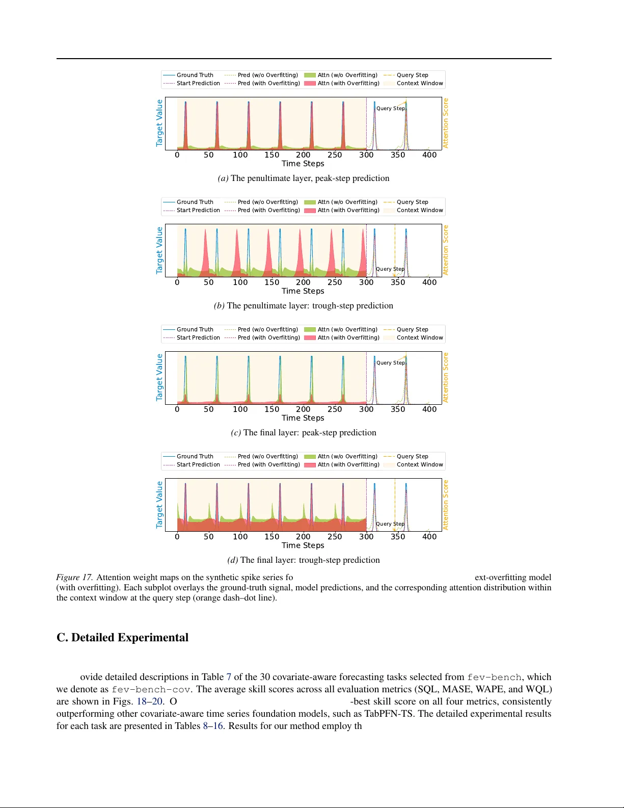
Baguan-TS: A Sequence-Nativ e In-Context Learning Model f or T ime Series F or ecasting with Cov ariates Linxiao Y ang 1 Xue Jiang 1 Gezheng Xu 1 Tian Zhou 1 Min Y ang 1 Zhaoyang Zhu 1 Linyuan Geng 1 Zhipeng Zeng 1 Qiming Chen 1 Xinyue Gu 1 Rong Jin 1 Liang Sun 1 Abstract T ransformers enable in-context learning (ICL) for rapid, gradient-free adaptation in time series fore- casting, yet most ICL-style approaches rely on tabularized, hand-crafted features, while end-to- end sequence models lack inference-time adapta- tion. W e bridge this gap with a uniﬁed frame w ork, Baguan-TS, which integrates the raw-sequence representation learning with ICL, instantiated by a 3D T ransformer that attends jointly o ver tem- poral, variable, and context axes. T o make this high-capacity model practical, we tackle two key hurdles: (i) calibration and training stabil- ity , improv ed with a feature-agnostic, tar get-space retriev al-based local calibration; and (ii) output ov ersmoothing, mitigated via conte xt-ov erﬁtting strategy . On public benchmark with covariates, Baguan-TS consistently outperforms established baselines, achie ving the highest win rate and sig- niﬁcant reductions in both point and probabilistic forecasting metrics. Further ev aluations across di verse real-world ener gy datasets demonstrate its robustness, yielding substantial impro vements. 1. Introduction T ime series forecasting increasingly demands models that adapt swiftly to new tasks, remain robust under distrib u- tion shift, and operate efﬁciently in data-limited regimes. While T ransformers ha v e re vealed the promise of in-context learning (ICL)—conditioning predictions on a small sup- port set at inference time without gradient updates—most ICL-style approaches in forecasting rely on tabularization and hand-crafted features ( Hoo et al. , 2025 ), limiting their ability to exploit the structure of raw sequences. On the other hand, end-to-end sequence models excel at learning representations directly from ra w time series b ut typically lack ICL-style, gradient-free adaptation ( Ansari et al. , 2024 ; 1 D AMO Academy , Alibaba Group, Hangzhou, China. . F igur e 1. Three paradigms for time series forecasting: (a) End-to- end sequence models learn from raw histories b ut lack in-context adaptation at inference. (b) T ab ular ICL approaches (e.g., T abPFN) perform ICL over feature-engineered representations. (c) Our uniﬁed approach (Baguan-TS) enables sequence-native ICL on raw multivariate inputs, attending ov er temporal, v ariables, and context for gradient-free adaptation. Das et al. , 2024 ). This disconnect motiv ates a framework that uniﬁes end-to-end representation learning with ICL for time series data, so that a single model can both extract features from raw sequences and adapt on the ﬂy . W e propose Baguan-TS, a general-purpose architecture that enables sequence-nativ e ICL on raw multiv ariate time se- ries without hand-crafted features. It builds on a uniﬁed, episodic framew ork that learns to forecast from raw se- quences gi ven a support set, thereby remo ving dependence on feature engineering while bringing ICL ’ s rapid adapta- tion into a sequence-nati ve architecture. An ov ervie w of this framew ork is shown in Fig. 1 . T o instantiate the framew ork, we introduce a 3D T ransformer that treats temporal, vari- able , and context dimensions as ﬁrst-class axes of attention. Analogous to video-style modeling, the model b uilds mul- tiscale representations over the temporal × variable plane and aligns support and query along the context axis via cross-attention. This design lifts the performance ceiling by discov ering task-rele v ant structure directly from raw time se- 1 Baguan-TS: A Sequence-Native In-Context Lear ning Model f or Time Series F orecasting with Co variates ries inputs and specializing predictions per episode through the provided context. In addition, the model admits a 2D inference mode by setting the context length to one, which functions as a strong complementary component in ensem- bles. In this way , it offers a robust fallback and diversity boost when integrating multiple predictors. Howe v er , adopting a high-capacity 3D architecture intro- duces two main challenges we tar get: Challenge 1: Locality Calibration. Large-capacity mod- els are prone to miscalibration and optimization insta- bility , especially when dealing with a large 3D T rans- former model. A lightweight, featur e-agnostic mecha- nism is needed to pro vide local , episode-speciﬁc cor - rection without manual features. Challenge 2: Output Oversmoothing in ICL. In the pre- sence of noisy , heterogeneous support examples, the model can oversmooth the spurious signals rather than extracting stable periodic rules. Effecti ve ICL under these conditions requires a careful balance between de- noising (resisting noise and shift) and selection (focus- ing on a compact, highly relev ant subset of samples). T o improv e calibration and stability , we propose a target- space retriev al-based forecast (Y -space RBfcst) local cal- ibration module. By referencing nearest support targets within each episode, this feature-agnostic procedure pro- vides a local, distribution-aware adjustment that comple- ments the learned predictor . It improv es calibration and stabilizes training and inference under limited per-task data and distribution shift, and integrates naturally with episodic ICL—offering a simple, retrie val-based bias/v ariance cor- rection that scales with model capacity without relying on hand-crafted features. T o counter output ov ersmoothing, we introduce a mitiga- tion strategy that integrates reliability-aw are weighting of support examples with deliberately o v erﬁtting to some ex- act context sample in the support set. Counterintuitiv ely , this concentrates attention on the few e xamples that matter for each query . This balance between denoising and selec- tion reduces spurious correlations and improv es few-shot robustness when training a lar ge 3D architecture. T ogether , these components form a uniﬁed framew ork that marries representation learning with ICL on raw se- quences; a 3D Transformer instantiation that raises the performance (and offers a practical 2D inference mode for ensemble complementarity); and two complementary mechanisms—context-o verﬁtting mitigation and Y -space RBfcst calibration—that make such a high-capacity , ICL- enabled model rob ust and trainable in practice. The result is a practical route to bringing ICL ’ s strengths to raw time 0.0 0.5 (Higher is better) Sundial- Base T oto -1.0 Moirai-2.0 Chr onos- Bolt T abPFN- TS T iR e x T imesFM-2.5 Ours A verage W in R ate (w .r .t SQL) 0.8 0.9 1.0 (L ower is better) Sundial- Base T oto -1.0 Moirai-2.0 Chr onos- Bolt T iR e x T abPFN- TS T imesFM-2.5 Ours A verage SQL F igure 2. Probabilistic forecasting results on fev-bench-cov (30 cov ariate-aware tasks): Baguan-TS leads all baselines, achiev- ing the highest av erage win rate and lo west av erage SQL. series forecasting under realistic data and shift conditions. W e summarize our contributions as follo ws: • W e propose Baguan-TS, a uniﬁed end-to-end frame- work that performs ICL directly on raw multiv ariate time series, without relying on feature engineering. It is instantiated as a 3D T ransformer attending jointly ov er temporal, v ariable, and context ax es, and also sup- ports a 2D inference mode. On fev-bench-cov (30 cov ariate-aware tasks), Baguan-TS achieves the best av erage scaled quantile loss (SQL) and MASE with the highest win rate, reducing SQL versus T abPFN-TS by 4.8% (Fig. 2 ). • W e dev elop a Y -space RBfcst local calibration module—feature-agnostic and episode-speciﬁc—that improv es calibration, data efﬁciency , and scalability when training larger 3D T ransformers. In our experi- ments, this module consistently improv es ov erall fore- casting accuracy and rob ustness under injected noise compared to training without retriev al. • W e introduce a context-ov erﬁtting strategy that explic- itly balances sample denoising and sample selection, stabilizing in-context learning in high-capacity mod- els. The strategy consistently lo wers training loss and restores periodic spike reconstruction, mitigating ov er- smoothing without harming trend accuracy . 2. Related W ork W e situate Baguan-TS within three lines of prior work, in- cluding end-to-end time series forecasting, large pretrained time series models, and in-context modeling. W e summa- rize the ke y capability dif ferences of Baguan-TS and these approaches in T able 1 . Time Series Forecasting . Deep neural networks domi- nate modern time series forecasting, with univ ariate models focusing on single sequences ( Rangapuram et al. , 2018 ; Salinas et al. , 2020 ; Oreshkin et al. , 2020 ) and multivari- ate models jointly modeling many correlated series using 2 Baguan-TS: A Sequence-Native In-Context Lear ning Model f or Time Series F orecasting with Covariates T able 1. Capability comparison of representati ve time series fore- casting approaches. Models Raw time sequence ICL (gradient- free) No hand- crafted features Cross- variable interaction Local retriev al-based calibration End-to-end models (PatchTST , FedFormer) ✓ × ✓ × × Large pretrained models (Chronos, TimesFM, T irex) ✓ × ✓ × × T abular ICL-style models (T abPFN-TS) × ✓ × ✓ × Ours (Baguan-TS) ✓ ✓ ✓ ✓ ✓ T ransformers ( W u et al. , 2021 ; Zhou et al. , 2022b ; Nie et al. , 2023 ; Liu et al. , 2024a ; W ang et al. , 2024b ; Chen et al. , 2024 ; Zhou et al. , 2023 ) and other architectures ( Sen et al. , 2019 ; Zhou et al. , 2022a ; Jin et al. , 2022 ; W ang et al. , 2024a ; Hu et al. , 2024 ; Qi et al. , 2024 ). While highly effecti ve on their training domains, these models typically require task- speciﬁc retraining, limiting their adaptability and moti v ating more general-purpose approaches. Large Pr etrained Time Series Models. Recent work pre- trains lar ge sequence models for time series ( W oo et al. , 2024 ; Goswami et al. , 2024 ; Ansari et al. , 2024 ; Das et al. , 2024 ; Rasul et al. , 2023 ; Liu et al. , 2024b ; Shi et al. , 2025 ), often with T ransformer-based architectures and di verse time series data. Howe ver , their zero- and few-shot performance, especially for multi v ariate forecasting with complex cross- channel dependencies, often still trails specialized models. In-Context Modeling. A complementary line of work treats forecasting as conditional generation and relies on in-context (few-shot) adaptation ( Hoo et al. , 2025 ; Feuer et al. , 2024 ; Zhu et al. , 2023 ; Dooley et al. , 2023 ; Hegsel- mann et al. , 2023 ). While competitive with strong tabular learners, these methods typically rely on hand-crafted fea- tures ( Chen & Guestrin , 2016 ; Ke et al. , 2017 ), limiting their practical usages in div erse applications. In contrast, the end- to-end sequence models are preferred by directly capturing temporal structures and cross-channel interactions. 3. Baguan-TS 3.1. Problem F ormulation In this paper, we consider univ ariate time series forecast- ing with known cov ariates. Let { y t } T t =1 be the observed series and { x t } T + H t =1 , where x t ∈ R M , the associated M - dimensional covariates, av ailable for both the history and the forecast horizon H (e.g., calendar ef fects or kno wn ex- ogenous inputs such as weather forecasts). The task is to predict the future values { y t } T + H t = T +1 . For a test instance, let y b = (y 1: T ) ∈ R T denote the look- back window , y f = (y T +1: T + H ) ∈ R H the future values, and X ∈ R ( T + H ) × M the co v ariates ov er t = 1 , . . . , T + H . W e assume an underlying mapping y f = f ∗ ( y b , X ) . In the in-context learning setting, we are gi ven a context set D c = { ( X j , y b j , y f j ) } C j =1 of C input–output examples. At test time, we adapt to a tar get instance by le veraging an inference function g to approximate f ∗ , where the approxi- mation is conditioned on D c to minimize the prediction error l ( y f , g ( X , y b , D c )) . Our objecti ve is to learn a univ ersal function g that can adapti vely ﬁt a wide range of dif ferent underlying mappings f ∗ across div erse tasks. For con venience, we concatenate covariates and the full series into Y i = [ X i , y i ] ∈ R ( T + H ) × ( M +1) , where y i ∈ R T + H stacks ( y b i , y f i ) . Stacking all context and target sam- ples yields a tensor Y ∈ R ( C +1) × ( T + H ) × ( M +1) , whose ﬁrst C slices correspond to D c and the last slice to the tar get instance. For the target slice, y f is unkno wn and stored as a mask, while it is observed for the conte xt slices. 3.2. Architectur e Fig. 3 shows the ov erall architecture of Baguan-TS, with its components detailed in the following subsections. 3 . 2 . 1 . P A T C H I N G A N D T O K E N I Z AT I O N Giv en the tensor Y ∈ R ( C +1) × ( T + H ) × ( M +1) , we apply an encoder based on temporal patching and random F ourier features ( Rahimi & Recht , 2007 ). Each variable in each slice is split along the temporal axis into S non-ov erlapping patches of length P (zero-padding the tail if needed), reduc- ing sequence length while preserving local structure. For each cov ariate patch q ∈ R P , we map it to e = [cos( ϕ ); sin( ϕ )] ∈ R D , with ϕ = Wq + b , where W and F igure 3. Overall architecture of Baguan-TS. The input tensor Y ∈ R ( C +1) × ( T + H ) × ( M +1) is encoded into patch t okens, then iterativ ely processed by stacked 3D Transformer blocks performing variable, temporal, and conte xt attention, and ﬁnally mapped by a prediction head to produce the forecasting outputs y f ∈ R H . 3 Baguan-TS: A Sequence-Native In-Context Lear ning Model f or Time Series F orecasting with Covariates b are shared learnable parameters. For the target series, we zero-ﬁll the unknown future and use a mask m ∈ { 0 , 1 } P to indicate observed positions. Its embedding e f adds an indicator term Vm to the Fourier features to distinguish the history from the forecast horizon. The resulting token tensor has shape ( C + 1) × S × ( M + 1) × D . 3 . 2 . 2 . 3 D T R A N S F O R M E R B L O C K The core of our architecture is the 3D T ransformer block, an encoder-only module that jointly models correlations across the v ariable, temporal, and conte xt dimensions. Given the encoded tokens, it applies a sequence of specialized atten- tion layers ov er these axes, follo wed by a feed-forward net- work (FFN). Residual connections and layer normalization follow each attention layer and the FFN. Compared to con ventional 1D or 2D T ransformer blocks ( Hoo et al. , 2025 ; Ansari et al. , 2024 ) that oper- ate on ﬂattened or reduced-dimensional embeddings, our block preserves a structured three-dimensional layout. This factorized design provides a stronger inducti ve bias while retaining the ﬂexibility of the standard T ransformer . Formally , let Z ∈ R ( C +1) × S × ( M +1) × D denote the token representation (contexts × temporal patches × variables × embedding dimension). All attention layers use standard multi-head self-attention (MHA) ( V aswani et al. , 2017 ) along different axes of this representation. W e describe these stages in detail below . T emporal Attention. This module learns temporal depen- dencies within each context to capture ho w patterns evolv e ov er time. For each ﬁxed context c and variable m , we extract the slice T c,m = Z c, : ,m, : ∈ R S × D as the representa- tion along the temporal axis. T o model these dependencies, we apply MHA integrated with Rotary Position Embed- dings (RoPE). By encoding relati ve phase information into the query and ke y vectors, RoPE allows the mechanism to naturally capture relative temporal distances and periodic patterns, which are crucial for time series forecasting. V ariable Attention: Instead of temporal sequences, this branch operates on the v ariable dimension V c,s = Z c,s, : , : ∈ R ( M +1) × D for each time step s . T o account for distinct variable semantics, we augment the representation with a learnable variable-wise embeddings before performing MHA to capture cross-variable correlations. Context Attention: This branch models relationships across dif ferent instances by taking the slice C s,m = Z : ,s,m, : ∈ R ( C +1) × D . Unlike the temporal and variable branches, context attention omits positional encodings, as the context dimension typically lacks an inherent sequential ordering and instead focuses on global information sharing. 3 . 2 . 3 . P R E D I C T I O N H E A D After a stack of 3D Transformer blocks, we obtain latent representations for future patches. A lightweight MLP head maps these features to per -horizon predicti ve distrib utions. Because inputs are z -normalized on the lookback (approxi- mately zero mean and unit v ariance), most forecast values lie within a bounded range; we ﬁx [ − 10 , 10] and uniformly discretize it into K = 5000 bins. For each horizon step, the head outputs logits over these bins; applying softmax yields a probability vector p ∈ R K . This pro vides a full probabilis- tic forecast with both point estimates (via the expected value ov er bin centers) and quantiles (via the empirical CDF). 3.3. T raining Our 3D Transformer operates on conte xt–target episode sets. During training, we (i) b uild these contexts via retrie v al- based forecasting; and (ii) stabilize in-context learning with a conte xt-ov erﬁtting strategy . Implementation details on training data, loss functions, and inference settings are in Appendix A . 3 . 3 . 1 . R E T R I E V A L - B A S E D F O R E C A S T I N G T o construct informative and scalable contexts, we adopt retriev al-based forecasting (RBfcst) to select informati ve contexts at scale. For a series of length N and a context win- dow T + H , there are N − T − H + 1 candidate subsequences of length T + H , so full enumeration is memory-intensi ve. Instead, giv en the target lookback y b ∈ R T as the query , we retriev e its K ctx nearest T -length subsequences from a sliding-window index over the historical region (to avoid leakage). Each retrie ved T -length windo w , together with the subsequent H points, forms one context of length T + H (with cov ariates aligned). Distances are computed on z - normalized windo ws (e.g., Euclidean or cosine), and K ctx is chosen to balance relev ance and memory . T o align training with this strategy and increase diversity , we ﬁrst select a reference sequence of length T + H , sam- ple a lookback of length T , and retriev e 2 K ctx nearest T - length subsequences using the same procedure. This leads to 2 K ctx + 1 candidates (including the selected reference), which is stacked into a tensor of shape (2 K ctx + 1) × S × ( M + 1) . W e then randomly choose K ctx slices to form a tensor of shape K ctx × S × ( M + 1) for that step. A sub- set of these K ctx slices is designated as the target (with its future masked), and the remainder serve as context. This randomized subsampling from a lar ger pool mimics imper- fect retriev al, encouraging context di versity and rob ustness to retriev al noise. Related tabular foundation models ( Thomas et al. , 2024 ; Xu et al. , 2025 ; Gorishniy et al. , 2024 ) typically retrie ve in covariate space (X-space). In contrast, we retrieve by 4 Baguan-TS: A Sequence-Native In-Context Lear ning Model f or Time Series F orecasting with Covariates covariates target Pre d ictio n ho r iz o n Contexts Organiza tion c ova r i a t e s t a r ge t target template co ntexts retr i e ve d by ta r g e t s i m i la r it y ( ) covariates target mos t simil ar con te xts sim=0.91 sim=0.92 sim=0.98 co ntexts retr i e ve d by co var iat e s sim il ari ty ( ) sim=0.92 sim=0.98 covariate template mos t simil ar con te xts uni forml y spl i t c on t ex ts ( ) i ii iii covariates target covariates target (a) Different conte xt organization strategies 1000 500 0 500 1000 t-SNE dim 1 1000 750 500 250 0 250 500 750 t-SNE dim 2 RBfcst (Y-space) RBfcst (X-space) No RBfcst Ground Truth 3 2 1 0 1 2 3 t-SNE dim 1 3 2 1 0 1 2 t-SNE dim 2 RBfcst (Y-space) RBfcst (X-space) No RBfcst Ground Truth (b) t-SNE visualization F igure 4. Context organization strate gies and t-SNE visualization. (a) Three context organization methods: (i) uniform splits ( green ); (ii) cov ariate-based retrieval in X-space ( purple , relies on feature engineering); (iii) target-based retrie val in Y -space (ours, yellow ), which focuses on historical patterns and is feature-agnostic. Higher similarity scores indicate stronger contextual relev ance. (b) t-SNE plots of prediction horizons on epf (top) and entsoe (bottom) for three RBfcst variants. The ground truth (red star) lies closest to the Y -space RBfcst cluster (shaded), indicating it best captures the true pattern. similarity of the target history (Y -space), i.e., nearest neigh- bors of the lookback segment. For time series, the trajectory often summarizes the combined ef fects of all driv ers, mak- ing Y -space retriev al more informativ e and feature-agnostic, without hand-crafted feature design. T o illustrate robustness, we compare three context- organization strategies in Fig. 4 : (i) uniform splitting (green), where windows are taken at equal intervals; (ii) X-space retriev al (purple), guided by covariate similarity and feature engineering; and (iii) Y -space retriev al (yellow , ours), which focuses on historical patterns most similar to the target. Higher similarity scores indicate stronger con- textual rele v ance. t-SNE plots on epf (top) and entsoe (bottom) show that horizons retrieved in Y -space cluster near the ground truth (red star), suggesting this strategy best captures the true pattern. 3 . 3 . 2 . C O N T E X T - O V E R FI T T I N G S T R A T E G Y The direct application of in-context learning to time series forecasting reveals a critical limitation: during early training, models tend to predict smooth, low-frequenc y trends while systematically suppressing periodic spike signals. This hap- pens even when identical spike patterns are clearly present in the context windo w , indicating that the model misinterprets such abrupt ﬂuctuations as noise rather than v alid signal components. Although this tendenc y may enhance rob ust- ness against irregular outliers in certain datasets, it sev erely undermines performance in time series domains where pe- riodic spikes constitute essential features (e.g., physiolog- ical monitoring or demand surges). T o mitigate this over - smoothing issue where the model fails to lev erage contextual spike templates for query inference, we introduce a context- ov erﬁtting strategy . Concretely , we enrich the query with a short segment copied verbatim from one context slice and add an auxiliary self-retrie v al objecti ve: the model is re- quired to identify and align the matching context segment and reconstruct the corresponding target v alues (see Fig. 5 , where we include a synthetic test sample x 2 whose lookback contains a motif duplicated from the context, and train the model to retrie ve that context). This explicitly encourages template matching: model must identify and retriev e target (a) Original design (b) Duplicate-context design F igure 5. Illustration of the context-overﬁtting strate gy . (a) Origi- nal design, where the model forecasts query targets from retrieved context episodes. (b) Duplicate-context design: a short segment from one context slice is copied into a query , and the model is trained to retriev e the matching context and reconstruct its targets. 5 Baguan-TS: A Sequence-Native In-Context Lear ning Model f or Time Series F orecasting with Covariates F igure 6. Effect of the context-o verﬁtting strategy . Main: train- ing loss curves for the baseline model (green) and our context- ov erﬁtting strategy (red). Insets: example forecasts compared with ground truth (blue). The baseline oversmooths outputs and misses high-frequency spikes (right); our strate gy keeps a lo w loss while recov ering spike patterns by matching contextual templates (left). val ues from the context when encountering identical patterns in the query . As demonstrated by the training dynamics and qualitati ve results in Fig. 6 , the baseline model underutilizes contextual templates and produces ov ersmoothed predic- tions, while our strategy enables accurate reconstruction of periodic spikes without compromising trend accuracy . 3.4. Adaptive Infer ence A key property of the 3D T ransformer is its structural ﬂexi- bility: it can operate either as a full sequence-nati ve model or as a 2D tabular-style predictor . Setting the context length S = 1 collapses the temporal axis and restrict attention to feature and context dimensions. W e ﬁnd this 2D mode useful when temporal dependence is mostly captured by cov ariates or is weak (e.g., unreliable history under distri- bution shift). Thus, we ensemble the 2D and 3D modes in inference, which consistently improv es SQL and reduces quantile calibration errors compared to using either mode alone. 4. Experiments 4.1. Experiment Settings W e compare Baguan-TS with recent time series founda- tion models: Sundial-Base ( Liu et al. , 2025b ), T abPFN- TS ( Hoo et al. , 2025 ), TimesFM-2.0 ( Das et al. , 2024 ), T iRex ( Auer et al. , 2025 ), T oto-1.0 ( Cohen et al. , 2025 ), Chronos-Bolt ( Ansari et al. , 2024 ), and Moirai-2.0 ( Liu et al. , 2025a ). Among them, only T abPFN-TS nativ ely supports cov ariates; models without cov ariate support are ev aluated on target-only inputs. W e report mean absolute scaled error (MASE), weighted ab- solute percentage error (W APE), scaled quantile loss (SQL), and weighted quantile loss (WQL), and the corresponding av erage win rates for each metric ( Shchur et al. , 2025 ), av- eraged over horizons and macro-averaged across datasets. Further details of the datasets, experimental setup, and addi- tional results are provided in Appendices B and C . 4.2. Zero-Shot F orecasting 4 . 2 . 1 . T I M E S E R I E S F O R E C A S T I N G W I T H C OV A R I A T E S Evaluation on public datasets. W e ﬁrst ev aluate Baguan- TS on the fev-bench benchmark ( Shchur et al. , 2025 ). Focusing on time series tasks with cov ariate information, we select 30 representative tasks from the 100 available datasets that provide at least one kno wn dynamic cov ariate, and refer to this subset as fev-bench-cov . W e ev aluate both point and probabilistic forecasting performance, com- paring Baguan-TS against leading time series foundation models. The results are reported in Fig. 2 and Figs. 18 – 20 (Appendix C.1 ). As shown in T able 2 , Baguan-TS con- sistently outperforms both univ ariate baselines, including T iRex and T oto-1.0, and models speciﬁcally designed for cov ariate-informed forecasting, such as T abPFN-TS. This demonstrates Baguan-TS can effecti vely le verage both his- torical target series and future covariates for accurate pre- dictions. T able 2. A verage results on fev-bench-cov . The best results are highlighted in bold , and the second-best results are underlined . Model SQL MASE W APE WQL Chronos-Bolt 0.9190 1.1233 0.2702 0.2181 Moirai-2.0 0.9202 1.1233 0.2750 0.2226 Sundial-Base 1.0172 1.1449 0.2813 0.2498 T imesFM-2.5 0.8276 1.0122 0.2592 0.2095 T abPFN-TS 0.8404 1.0430 0.2015 0.1643 T iRex 0.8927 1.1081 0.2753 0.2233 T oto-1.0 0.9600 1.1755 0.2737 0.2248 Ours 0.7997 0.9857 0.2173 0.1724 Evaluation on real-w orld applications. W e further ev al- uate Baguan-TS on 27 real-world datasets with historical and future covariates (e.g., weather , calendar). T able 3 re- ports av erages ov er all datasets. Among the baselines, only T abPFN-TS and Baguan-TS use covariates; the others op- erate on the target series only . Baguan-TS achiev es the best ov erall SQL, MASE, W APE, and WQL, improving ov er T abPFN-TS and all non-covariate baselines, indicating more effecti ve use of contextual signals. Detailed dataset descriptions and experimental results are provided in the Appendix C.1 . 4 . 2 . 2 . U N I V A R I A T E T I M E S E R I E S F O R E C A S T I N G W e ne xt consider uni variate time series forecasting with- out cov ariates, where Baguan-TS adapts by incorporating null or time-only feature columns. Speciﬁcally , we ev alu- ated 10 tasks from the fev-bench-mini dataset ( Shchur et al. , 2025 ), where multi variate datasets are ﬂattened into standard univ ariate forecasting problems; we refer to this subset as fev-bench-uni . As shown in Fig. 7 , Baguan- TS achie ves competiti ve macro-av eraged SQL across tasks ev en without cov ariates. Notably , it outperforms T abPFN- 6 Baguan-TS: A Sequence-Native In-Context Lear ning Model f or Time Series F orecasting with Covariates T able 3. A verage results on real-world application datasets. The best results are highlighted in bold , and the second-best results are underlined. Model SQL MASE W APE WQL Chronos-Bolt 0.5101 0.6350 0.0976 0.0783 Moirai-2.0 0.7139 0.8875 0.1031 0.0860 Sundial-Base 0.7486 0.9042 0.1133 0.0981 T abPFN-TS 0.4663 0.6115 0.0688 0.0537 T imesFM-2.0 0.8418 0.9278 0.1093 0.0954 T iRex 0.5710 0.7094 0.0975 0.0784 T oto-1.0 0.8414 1.0566 0.1269 0.1034 Ours 0.3974 0.4956 0.0597 0.0490 0.0 0.5 (Higher is better) Sundial- Base Chr onos- Bolt T abPFN- TS Ours T oto -1.0 T iR e x Moirai-2.0 T imesFM-2.5 A verage W in R ate (w .r .t SQL) 0.4 0.5 0.6 (L ower is better) Chr onos- Bolt T abPFN- TS Sundial- Base T oto -1.0 T iR e x Ours T imesFM-2.5 Moirai-2.0 A verage SQL F igure 7. Evaluation on fev-bench-uni (10 univ ari- ate/multiv ariate tasks). Baguan-TS achiev es competiti ve prob- abilistic forecasting performance on tasks without cov ariates. TS, which also nati vely supports cov ariates, on more than 50% of these datasets; it also achie ves SO T A performance in terms of macro-a veraged W APE and WQL (see Fig. 21 , Appendix C.2 ). These results indicate strong macro-lev el stability and robustness on aggre gate-sensiti ve metrics, high- lighting system-lev el accuracy . 4.3. Ablation Study 4 . 3 . 1 . E FF E C T O F R B F C S T W e ﬁrst ablate the proposed RBfcst module on an energy task ( entsoe 1h ) and a retail task ( hermes ). The base- line (w/o RBfcst) uses uniformly split contexts. W e compare three retriev al variants: X-space (cov ariates), XY -space (co- variates + targets), and our Y -space RBfcst (targets only). All v ariants use the a verage of cosine and L 2 distances for segment similarity . As shown in T able 4 , Y -space RBfcst consistently outper- forms both X-space and XY -space variants, all of which signiﬁcantly surpass the w/o RBfcst baseline. This vali- dates the critical role of RBfcst in ICL-based time series forecasting and conﬁrms that historical target trajectories generally provide more informati ve conte xt than cov ariates, without requiring sophisticated feature selection or aggrega- tion mechanisms. The performance advantage of Y -space RBfcst is particularly large on entsoe 1h , whereas the gap is smaller on hermes , which has shorter lookback windows and sparser co variates. T able 4. Probabilistic and point forecasting ev aluation for different RBfcst variants on entsoe 1H and hermes datasets. Method entsoe 1H hermes SQL MASE W APE WQL SQL MASE W APE WQL w/o RBfcst 0.4284 0.5387 0.0328 0.0262 0.6607 0.8445 0.0032 0.0025 X-space 0.4185 0.5178 0.0313 0.0256 0.6186 0.7973 0.0030 0.0023 XY -space 0.4005 0.4972 0.0297 0.0241 0.6186 0.7972 0.0030 0.0023 Y -space 0.3859 0.4819 0.0287 0.0231 0.6185 0.7971 0.0030 0.0023 N o i s e S c a l e ( ) 0.35 0.40 0.45 0.50 SQL Gaussian White Noise N o i s e S c a l e ( ) 0.4 0.5 0.6 0.7 R andom W alk Noise N o i s e S c a l e ( ) 0.35 0.40 0.45 0.50 0.55 P eriodic Noise Ours (XY -space RBfcst) Ours (X -space RBfcst) Ours (Y -space RBfcst) T abPFN- TS F igure 8. Robustness ev aluation on epf fr under Gaussian white noise, random walk noise, and periodic noise, with κ ∈ { 0 , 0 . 05 , 0 . 1 , 0 . 2 , 0 . 4 , 0 . 6 , 0 . 8 , 1 . 0 } . T o further e valuate the robustness of our local calibra- tion module, we conduct noise-injection experiments on epf fr using three representative noise types: (i) Gaus- sian white noise (stationary); (ii) random walk noise (non- stationary with trend); and (iii) periodic noise (seasonal interference). The noise intensity is controlled by a scaling factor κ relativ e to the series’ empirical standard devia- tion (see Appendix B.2 for details). As shown in Fig. 8 , although T abPFN-TS achieves the best SQL in the clean setting ( κ = 0 ), its performance degrades sharply under stationary Gaussian noise as κ increases (especially when κ ≥ 0 . 1 ). In contrast, Baguan-TS maintains stable perfor- mance across all noise types and intensities. Notably , the Y -space RBfcst variant exhibits the highest robustness, with minimal performance drop e ven at high noise le vels. This shows that our feature-agnostic locality calibration effec- tiv ely mitigates the impact of div erse external perturbations. 4 . 3 . 2 . E FF E C T O F C O N T E X T - O V E R FI T T I N G W e ablate the proposed context-ov erﬁtting strategy by re- training two models (a full model with context-o verﬁtting and a baseline without it) from scratch for 220K steps on a dataset with clear daily and weekly seasonality and periodic spikes. Fig. 6 sho ws training loss es and qualitati ve forecasts. W ith context-o verﬁtting, the training loss is consistently lower—unsurprising, as the auxiliary self-retrie val task (re- cov ering targets for a query containing a duplicated context segment) is easier than forecasting unseen tar gets. More importantly , without context-o verﬁtting the forecasts are ov erly smooth and miss most spikes, while the full model 7 Baguan-TS: A Sequence-Native In-Context Lear ning Model f or Time Series F orecasting with Covariates 1 2 5 10 50 100 k (lar ger = sharper) 0.2 0.8 1.4 RMSE (L ower is Better) w/o Overfitting with Overfitting P erfor mance Gap (a) RMSE vs. Spike Sharpness 0 50 100 150 200 T ime Steps T ar get V alue Query Step Gr ound T ruth Start P r ediction Query Step Conte xt W indow P r ed (w/o Overfitting) P r ed (with Overfitting) A ttn (w/o Overfitting) A ttn (with Overfitting) A ttention Scor e (b) Attention W eight Map F igure 9. Ablation of the conte xt-overﬁtting strategy . (a) The full model (red) consistently outperforms the baseline (green) on synthetic periodic spike data for all k , where larger k corresponds to sharper spikes. (b) Attention map for a representativ e peak step (orange dotted line). captures much more high-frequenc y structure and accurately predicts the periodic spikes without distorting the trend. T o further assess robustness and clarify the mechanism, we compare these two models on synthetic periodic toy data. As shown in Fig. 9a , the full model substantially reduces RMSE and more consistently recovers periodic spikes from the lookback windo w . T o examine attention behavior , Fig. 9b visualizes a local attention map: with context-ov erﬁtting, the peak step attends strongly to historical peaks, whereas the baseline exhibits a pronounced dip at these locations, supporting our explanation of over -smoothing in vanilla attention. Details of the data generation and additional visualizations are provided in Appendix B.3 . 4 . 3 . 3 . D I FF E R E N T I N F E R E N C E M O D E S In this section, we compare the 2D, 3D, and ensemble in- ference modes. A veraged results on the fev-bench-cov are presented in T able 5 . While the standalone 3D and 2D modes already deli ver strong performance, their ensemble consistently improv es all metrics for both point and proba- bilistic forecasting. T o understand these gains, we compute the Pearson correlation between 2D and 3D residuals pooled across all tasks (Fig. 10a ), obtaining 0.75. This conﬁrms that both modes are accurate and successfully capture the dominant temporal dynamics, while the correlation being well below 1.0 indicates di verse error structures. T o further visualize this diversity , we plot the joint residual distribution for the entsoe 1H task in Fig. 10b , where points in the second and fourth quadrants highlight opposite-signed resid- uals, suggesting complementary errors. W e also ev aluate T able 5. A verage results on fev-bench-cov under different inference modes of Baguan-TS model. Model SQL MASE W APE WQL Ours (2D mode) 0.8769 1.0705 0.2333 0.1863 Ours (3D mode) 0.8333 1.0220 0.2285 0.1830 Ours (Ensemble) 0.7997 0.9857 0.2173 0.1724 2D mode 3D mode 2D mode 3D mode 1.00 0.75 0.75 1.00 (a) Heatmap 0.1 0.0 0.1 2D R esiduals 0.1 0.0 0.1 3D R esiduals (b) Residual Correlation F igure 10. Residual correlation analysis of 2D and 3D in- ference modes. (a) Aggregated Pearson correlation across 30 tasks in fev-bench-cov . (b) Joint residual distribution for entsoe 1H , where darker blue bins indicate higher data density . Points along the red dashed identity line ( y = x ) represent cases in which the errors in both modes are equal. Deviations from this diagonal, particularly in the second and fourth quadrants, highlight the complementary error structures between the two modes. the probabilistic calibration using calibration histograms (Fig. 11 ) ( Gneiting et al. , 2007 ). The x-axis shows ground- truth quantile levels under predicted CDFs; perfectly cali- brated models yield a uniform histogram. W e observe oppo- site systematic biases in the base modes: the 2D mode sho ws a peaked histogram indicating under -conﬁdent predictions, whereas the 3D mode exhibits a U-shape distribution with ov er-conﬁdence. The ensemble mode balances these errors, yielding a near-uniform histogram for better calibration. 0.0 0.5 1.0 Quantile L evel 0.00 0.05 0.10 0.15 F r equency 2D Mode 0.0 0.5 1.0 Quantile L evel 3D Mode 0.0 0.5 1.0 Quantile L evel Ensemble F igure 11. Calibration histograms of ground-truth quantile lev els in predicted CDFs for dif ferent inference modes on entsoe 1H . A well-calibrated model yields a uniform histogram (red dashed line). The 2D mode is under-conﬁdent (peaked), the 3D mode is over -conﬁdent (U-shaped), whereas the ensemble effecti vely cancels these biases and approaches the ideal uniform distribution. 5. Conclusion W e presented Baguan-TS, a uniﬁed frame work that brings in-context learning to raw time series by combining a 3D T ransformer o ver temporal, variable, and conte xt ax es with a practical 2D+3D inference scheme. A target-space retrie v al- based calibration module and a context-ov erﬁtting strat- egy make this high-capacity architecture more stable, bet- ter calibrated, and less prone to oversmoothing. Across fev-bench-cov , fev-bench-uni and 27 in-house datasets, Baguan-TS consistently exhibits strong perfor- mance, sho wing that raw-sequence ICL can be both effecti ve and robust in realistic forecasting settings. 8 Baguan-TS: A Sequence-Native In-Context Lear ning Model f or Time Series F orecasting with Covariates References Aksu, T ., W oo, G., Liu, J., Liu, X., Liu, C., Savarese, S., Xiong, C., and Sahoo, D. Gift-eval: A benchmark for general time series forecasting model e valuation. arXiv pr eprint arXiv:2410.10393 , 2024. Ansari, A. F ., Stella, L., T urkmen, C., Zhang, X., Mercado, P ., Shen, H., Shchur , O., Rang apuram, S. S., Arango, S. P ., Kapoor , S., et al. Chronos: Learning the language of time series. arXiv preprint , 2024. Auer , A., Podest, P ., Klotz, D., B ¨ ock, S., Klambauer, G., and Hochreiter , S. Tire x: Zero-shot forecasting across long and short horizons with enhanced in-context learning. arXiv pr eprint arXiv:2505.23719 , 2025. Chang, K.-M. Arrhythmia ECG noise reduction by en- semble empirical mode decomposition. Sensors , 10(6): 6063–6080, 2010. Chen, P ., Zhang, Y ., Cheng, Y ., Shu, Y ., W ang, Y ., W en, Q., Y ang, B., and Guo, C. P athformer: Multi-scale transform- ers with adaptiv e pathways for time series forecasting. In Pr oceedings of the International Conference on Learning Repr esentations , 2024. Chen, T . and Guestrin, C. XGBoost: A scalable tree boost- ing system. In Proceedings of the 22nd A CM SIGKDD International Confer ence on Knowledge Discovery and Data Mining , pp. 785–794, 2016. Cohen, B., Khwaja, E., Doubli, Y ., Lemaachi, S., Lettieri, C., Masson, C., Miccinilli, H., Ram ´ e, E., Ren, Q., Ros- tamizadeh, A., et al. This time is dif ferent: An observ abil- ity perspecti ve on time series foundation models. arXiv pr eprint arXiv:2505.14766 , 2025. Das, A., Kong, W ., Sen, R., and Zhou, Y . A decoder-only foundation model for time-series forecasting. In Pr oceed- ings of the 41st International Conference on Machine Learning , 2024. Dooley , S., Khurana, G. S., Mohapatra, C., Naidu, S. V ., and White, C. ForecastPFN: Synthetically-trained zero-shot forecasting. Advances in Neural Information Pr ocessing Systems , 36:2403–2426, 2023. Feuer , B., Schirrmeister, R. T ., Cherepanova, V ., Hegde, C., Hutter , F ., Goldblum, M., Cohen, N., and White, C. T uneTables: Context optimization for scalable prior - data ﬁtted networks. Advances in Neural Information Pr ocessing Systems , 37:83430–83464, 2024. Gneiting, T ., Balabdaoui, F ., and Raftery , A. E. Probabilistic forecasts, calibration and sharpness. Journal of the Royal Statistical Society Series B: Statistical Methodology , 69 (2):243–268, 2007. Gorishniy , Y ., Rubachev , I., Kartashe v , N., Shlenskii, D., K otelnikov , A., and Babenko, A. T abR: T abular deep learning meets nearest neighbors. In Pr oceedings of the 12th International Confer ence on Learning Repr esenta- tions , 2024. Goswami, M., Szafer , K., Choudhry , A., Cai, Y ., Li, S., and Dubrawski, A. MOMENT: A family of open time- series foundation models. In Pr oceedings of the 41st International Confer ence on Machine Learning , 2024. Hegselmann, S., Buendia, A., Lang, H., Agrawal, M., Jiang, X., and Sontag, D. T abLLM: Fe w-shot classiﬁcation of tabular data with large language models. In Pr oceed- ings of the 26th International Confer ence on Artiﬁcial Intelligence and Statistics , pp. 5549–5581, 2023. Hoo, S. B., M ¨ uller , S., Salinas, D., and Hutter , F . The tab ular foundation model TabPFN outperforms specialized time series forecasting models based on simple features. arXiv pr eprint arXiv:2501.02945 , 2025. Hu, J., Hu, Y ., Chen, W ., Jin, M., Pan, S., W en, Q., and Liang, Y . Attractor memory for long-term time series forecasting: A chaos perspective. Advances in Neural Information Pr ocessing Systems , 37:20786–20818, 2024. Jin, M., Zheng, Y ., Li, Y .-F ., Chen, S., Y ang, B., and Pan, S. Multiv ariate time series forecasting with dynamic graph neural odes. IEEE T ransactions on Knowledge and Data Engineering , 35(9):9168–9180, 2022. Ke, G., Meng, Q., Finley , T ., W ang, T ., Chen, W ., Ma, W ., Y e, Q., and Liu, T .-Y . LightGBM: A highly efﬁcient gradient boosting decision tree. Advances in Neural In- formation Pr ocessing Systems , 30, 2017. Kim, G. I. and Chung, K. Extraction of features for time series classiﬁcation using noise injection. Sensors , 24 (19):6402, 2024. Kim, T ., Kim, J., T ae, Y ., Park, C., Choi, J.-H., and Choo, J. Re versible instance normalization for accurate time-series forecasting against distrib ution shift. In Pr oceedings of the International Conference on Learning Repr esenta- tions , 2022. Liu, C., Aksu, T ., Liu, J., Liu, X., Y an, H., Pham, Q., Sahoo, D., Xiong, C., Sav arese, S., and Li, J. Moirai 2.0: When less is more for time series forecasting. arXiv pr eprint arXiv:2511.11698 , 2025a. Liu, Y ., Hu, T ., Zhang, H., W u, H., W ang, S., Ma, L., and Long, M. iTransformer: In verted transformers are ef fec- ti ve for time series forecasting. In Pr oceedings of the 12th International Confer ence on Learning Repr esentations , 2024a. 9 Baguan-TS: A Sequence-Native In-Context Lear ning Model f or Time Series F orecasting with Covariates Liu, Y ., Zhang, H., Li, C., Huang, X., W ang, J., and Long, M. T imer: Generati ve pre-trained transformers are lar ge time series models. In Pr oceedings of the 41st International Confer ence on Machine Learning , 2024b. Liu, Y ., Qin, G., Shi, Z., Chen, Z., Y ang, C., Huang, X., W ang, J., and Long, M. Sundial: A family of highly capable time series foundation models. arXiv preprint arXiv:2502.00816 , 2025b. Nie, Y ., Nguyen, N. H., Sinthong, P ., and Kalagnanam, J. A time series is worth 64 words: Long-term forecasting with transformers. In Pr oceedings of the 11th International Confer ence on Learning Representations , 2023. Oreshkin, B. N., Carpov , D., Chapados, N., and Bengio, Y . N-beats: Neural basis expansion analysis for inter- pretable time series forecasting. In Proceedings of the International Confer ence on Learning Repr esentations , 2020. Qi, S., Xu, Z., Li, Y ., W en, L., W en, Q., W ang, Q., and Qi, Y . PDETime: Rethinking long-term multiv ariate time series forecasting from the perspective of partial differential equations. arXiv preprint , 2024. Rahimi, A. and Recht, B. Random features for large-scale kernel machines. Advances in Neural Information Pr o- cessing Systems , 20, 2007. Rangapuram, S. S., Seeger , M. W ., Gasthaus, J., Stella, L., W ang, Y ., and Januschowski, T . Deep state space models for time series forecasting. Advances in Neural Information Pr ocessing Systems , 31, 2018. Rasul, K., Ashok, A., W illiams, A. R., Khorasani, A., Adamopoulos, G., Bhagwatkar , R., Bilo ˇ s, M., Ghonia, H., Hassen, N. V ., Schneider , A., Garg, S., Drouin, A., Chapados, N., Ne vmyv aka, Y ., and Rish, I. Lag-Llama: T ow ards foundation models for time series forecasting. arXiv pr eprint arXiv:2310.08278 , 2023. Salinas, D., Flunkert, V ., Gasthaus, J., and Januschowski, T . DeepAR: Probabilistic forecasting with autoregressi ve recurrent networks. International Journal of F orecasting , 36(3):1181–1191, 2020. Sen, R., Y u, H.-F ., and Dhillon, I. S. Think globally , act locally: A deep neural network approach to high- dimensional time series forecasting. Advances in Neural Information Pr ocessing Systems , 32:4837–4846, 2019. Shchur , O., Ansari, A. F ., T urkmen, C., Stella, L., Erickson, N., Guerron, P ., Bohlk e-Schneider , M., and W ang, Y . Fev- bench: A realistic benchmark for time series forecasting. arXiv pr eprint arXiv:2509.26468 , 2025. Shi, X., W ang, S., Nie, Y ., Li, D., Y e, Z., W en, Q., and Jin, M. Time-MoE: Billion-scale time series foundation models with mixture of experts. Proceedings of the Inter - national Confer ence on Learning Representations , 2025. Thomas, V ., Ma, J., Hosseinzadeh, R., Golestan, K., Y u, G., V olko vs, M., and Caterini, A. Retriev al & ﬁne-tuning for in-context tab ular models. Advances in Neur al Informa- tion Pr ocessing Systems , 37:108439–108467, 2024. V aswani, A., Shazeer , N., Parmar , N., Uszkoreit, J., Jones, L., Gomez, A. N., Kaiser , Ł ., and Polosukhin, I. Atten- tion is all you need. Advances in Neural Information Pr ocessing Systems , 30, 2017. W ang, S., Li, C., and Lim, A. A model for non-stationary time series and its applications in ﬁltering and anomaly detection. IEEE T ransactions on Instrumentation and Measur ement , 70:1–11, 2021. W ang, S., W u, H., Shi, X., Hu, T ., Luo, H., Ma, L., Zhang, J. Y ., and Zhou, J. T imeMixer: Decomposable multiscale mixing for time series forecasting. In Pr oceedings of the International Confer ence on Learning Repr esentations , 2024a. W ang, X., Zhou, T ., W en, Q., Gao, J., Ding, B., and Jin, R. CARD: Channel aligned robust blend transformer for time series forecasting. In Proceedings of the Interna- tional Confer ence on Learning Representations , 2024b. W oo, G., Liu, C., Kumar , A., Xiong, C., Savarese, S., and Sahoo, D. Uniﬁed training of uni versal time series fore- casting transformers. In Proceedings of the International Confer ence on Machine Learning , 2024. W u, H., Xu, J., W ang, J., and Long, M. Autoformer: Decom- position transformers with auto-correlation for long-term series forecasting. Advances in Neural Information Pr o- cessing Systems , 34:22419–22430, 2021. Xu, D., Cirit, O., Asadi, R., Sun, Y ., and W ang, W . Mixture of in-context prompters for tabular PFNs. Proceedings of the International Confer ence on Learning Representa- tions , 2025. Zhou, T ., Ma, Z., W en, Q., Sun, L., Y ao, T ., Y in, W ., Jin, R., et al. Film: Frequency improved legendre memory model for long-term time series forecasting. Advances in Neural Information Pr ocessing Systems , 35:12677– 12690, 2022a. Zhou, T ., Ma, Z., W en, Q., W ang, X., Sun, L., and Jin, R. FEDformer: Frequency enhanced decomposed trans- former for long-term series forecasting. In Pr oceedings of the International Confer ence on Machine Learning , 2022b. 10 Baguan-TS: A Sequence-Native In-Context Lear ning Model f or Time Series F orecasting with Covariates Zhou, T ., Niu, P ., Sun, L., Jin, R., et al. One ﬁts all: Power general time series analysis by pretrained LM. Advances in Neural Information Pr ocessing Systems , 36:43322– 43355, 2023. Zhu, B., Shi, X., Erickson, N., Li, M., Karypis, G., and Shoaran, M. Xtab: Cross-table pretraining for tabular transformers. In Proceedings of the International Confer - ence on Machine Learning , 2023. 11 Baguan-TS: A Sequence-Native In-Context Lear ning Model f or Time Series F orecasting with Covariates A. Implement details A.1. Model Details Baguan-TS uses a 3D T ransformer-based architecture with h yperparameters summarized in T able 6 . The model has 22.4 million parameters. T able 6. Baguan-TS model architecture hyperparameters. Parameter V alue T emporal patch size ( P ) 8 Number of 3D T ransformer blocks ( L ) 12 Number of heads 6 Embedding dimension ( D ) 192 Feed-forward dimension 768 Output dimension ( K ) 5000 During training, C , T , H , and M are randomly sampled for each batch, up to ﬁx ed maximum values. W e set C max = 50 for the contexts, T max = 2048 for the lookback length, H max = 192 for the prediction horizon, and M max = 80 for the number of cov ariates. A.2. T raining Data T raining data is critical to the performance of a foundation model. Baguan-TS is trained on a mixture of synthetic data and real-world benchmark data. The real-world data provide grounding in practical distributions and noise characteristics, while the synthetic data are designed to span a broad family of dynamics, cov ariate roles, and latent-factor structures that are hard to obtain exhausti vely from any single corpus. Synthetic Data. The div erse and task-speciﬁc semantics of cov ariates in different forecasting tasks make it difﬁcult to handcraft a single, general-purpose synthetic data simulator . Our key idea is that man y cov ariate-aware forecasting problems can be vie wed as regression with partially observed, time-correlated latent factors. Observ ed cov ariates are noisy or incomplete proxies for these latent dri vers, while the tar get series combines autoregressiv e structure with nonlinear effects of both observed and latent inputs. Accordingly , we build a generic generator in which latent trajectories are drawn from a kernel dictionary , and transformed through a dynamic structural causal mechanism with a random MLP to induce nonlinear interactions. Only a subset of nodes is exposed as observed cov ariates and the remainder act as unobserved dri vers; process and measurement noise, as well as optional regime shifts, are added to simulate dif ferent data characteristics. Within each task, the mechanism (graph, MLP weights, kernels, noise scales, exposure set) is ﬁxed, whereas context and tar get instances draw independent latent realizations. Real-W orld Data. W e include the GIFT -Eval pretraining corpus ( Aksu et al. , 2024 ) in our training set and augment each time step with a time index feature. T o simulate distribution shifts and expose the model to regime changes, we concatenate multiple normalized series into longer sequences and randomly sample contiguous subsequences as training examples. A.3. T raining Loss W e use the continuous ranked probability score (CRPS) as the training loss. For a predictiv e CDF F and observation y , CRPS ( F , y) = R ∞ −∞ ( F (z) − I (z ≥ y)) 2 d z . When the predictiv e distribution is represented by K bins with centers h i , we collect the probabilities into a vector p = (p 1 , . . . , p K ) ⊤ ∈ R K with P i p i = 1 , the corresponding discrete form of each time step is CRPS = K X i =1 p i | h i − y | − 1 2 K X i =1 K X j =1 p i p j | h i − h j | , (1) where the ﬁrst term is the expected absolute error under the forecast and the second term equals half the expected pairwise absolute distance between two independent forecast draws, acting as a sharpness term that discourages o ver -dispersion while preserving propriety . W e compute CRPS per horizon step and av erage across the forecast windo w . 12 Baguan-TS: A Sequence-Native In-Context Lear ning Model f or Time Series F orecasting with Covariates A.4. Inference Details For the inference process, we implement a stochastic ensemble approach to enhance prediction robustness through input perturbation and multiple forward passes. Speciﬁcally , cov ariate column positions are randomly shufﬂed, and 20% of historical target values are masked during each inference iteration, with 2–4 independent forward passes performed. The output is the av erage of these forward passes. In our experimental frame work, a v alidation set is constructed for each time series by rolling the historical windo w backward by either 2 or 5 steps to simulate realistic forecasting conditions. The ﬁnal predictions represent an ensemble of 2–9 distinct conﬁgurations selected based on their performance on this validation set. These conﬁgurations vary across four critical dimensions: • Inference mode (2D/3D/2D+3D ensemble); • Whether to include time series order , a blank column, or calendar-speciﬁc temporal features (e.g., year , month, day); • Whether to apply rev ersible instance normalization (RevIn) ( Kim et al. , 2022 ) to each or ganized context; • Context window length ( T ), deﬁned as an integer multiple of the prediction horizon, taking v alues from 2 to 14. This ensemble strategy enhances architectural div ersity , automatically addresses cov ariate-agnostic scenarios by prioritizing temporal pattern extraction, and mitigates the uncertainty caused by the changeable conte xt length and RBfcst module. B. Details of Ablation Study B.1. Effect of 3D and 2D Ensemble Residual Analysis for Point Prediction. W e analyze the residual correlation between the 2D and 3D inference modes across all 30 cov ariate-aware tasks in the fev-bench dataset. The per-task Pearson correlation ranges from 0.42 to 0.95, with an aggre gated v alue of 0.75 (Fig. 10a ). The aggregated joint residual distribution is shown in Fig. 12c , re vealing div erse error patterns that further support the effecti veness of combining 2D and 3D inference modes. 0.1 0.0 0.1 2D R esiduals 0.1 0.0 0.1 3D R esiduals (a) proenfo gfc14 0.1 0.0 0.1 2D R esiduals 0.1 0.0 0.1 3D R esiduals (b) rossmann 1W 0.05 0.00 0.05 2D R esiduals 0.05 0.00 0.05 3D R esiduals (c) Aggregation across 30 tasks F igure 12. Joint residual distributions for the ener gy task proenfo gfc14 , the retail task rossmann 1W , and the aggregated results across all 30 tasks. Darker blue bins indicate higher data density . Points lying along the red dashed identity line ( y = x ) correspond to instances where prediction errors are equal in both modes. Deviations from this diagonal, particularly in the second and fourth quadrants, rev eal complementary error patterns between the two modes. Calibration Analysis for Probabilistic Analysis. T o assess the ef fectiv eness and complementarity of the 2D and 3D inference modes, we analyze their probabilistic calibration. W e compute histograms of the ground-truth quantile lev els, also known as Probability Inte gral T ransform (PIT) histograms. Speciﬁcally , for each observation y t and predicted CDF ˆ F t , the quantile level is giv en by u t = ˆ F t (y t ) . The x-axis represents these quantile lev els ranging from 0 to 1, while the y-axis (labeled “Frequency”) indicates the relati ve frequenc y of ground truths falling into each quantile bin. A perfectly calibrated model should yield a uniform distribution, visualized as a ﬂat line at Frequenc y = 0.1. As shown in Figs. 13 – 15 , the 2D and 3D modes exhibit di verse error structures across different tasks. On the epf de task (Fig. 13 ), the 2D mode shows a distinct decreasing trend, indicating a systematic positiv e bias (ov er-estimation), as ground 13 Baguan-TS: A Sequence-Native In-Context Lear ning Model f or Time Series F orecasting with Covariates truths frequently fall into lower quantiles. Con versely , the 3D mode displays an increasing trend, indicating a negati ve bias. These opposing biases ef fecti vely cancel out in the ensemble mode, resulting in a well-calibrated histogram. On the hermes task (Fig. 14 ), the 2D mode shows a U-shaped distrib ution, indicating ov er-conﬁdent predictions. In contrast, the 3D mode demonstrates superior calibration performance. Aggregated across all tasks (Fig. 15 ), the 2D mode consistently exhibits a U-shaped pattern, reﬂecting overconﬁdent predictions with under-dispersed distrib utions, whereas the 3D mode maintains more stable calibration performance with slight under -conﬁdence. The ensemble strategy ef fecti vely mitigates their weaknesses, resulting in robust probabilistic performance. 0.0 0.5 1.0 Quantile L evel 0.00 0.05 0.10 0.15 F r equency 2D Mode 0.0 0.5 1.0 Quantile L evel 3D Mode 0.0 0.5 1.0 Quantile L evel Ensemble F igure 13. Calibration histograms of ground-truth quantile lev els in predicted CDFs for dif ferent inference modes on epf de (energy task). 0.0 0.5 1.0 Quantile L evel 0.0 0.1 0.2 F r equency 2D Mode 0.0 0.5 1.0 Quantile L evel 3D Mode 0.0 0.5 1.0 Quantile L evel Ensemble F igure 14. Calibration histograms of ground-truth quantile levels in predicted CDFs for dif ferent inference modes on hermes (retail task). 0.0 0.5 1.0 Quantile L evel 0.00 0.05 0.10 0.15 F r equency 2D Mode 0.0 0.5 1.0 Quantile L evel 3D Mode 0.0 0.5 1.0 Quantile L evel Ensemble F igure 15. Calibration histograms of ground-truth quantile levels in predicted CDFs for different inference modes on fev-bench-cov dataset (across all 30 tasks). B.2. Robustness to Injected Noise T o more rigorously ev aluate the robustness and stability of the proposed local calibration module, we conduct a noise injection experiment on the epf fr dataest. Speciﬁcally , we corrupt the original time series with three types of synthetic stochastic noise: Gaussian white noise, random walk noise, and periodic noise ( Chang , 2010 ; Kim & Chung , 2024 ; W ang et al. , 2021 ). For each noise type, the intensity is controlled by a scaling factor κ ∈ { 0 . 05 , 0 . 1 , 0 . 2 , 0 . 4 , 0 . 6 , 0 . 8 , 1 . 0 } . The actual scale parameter used is deﬁned as σ · κ , where σ denotes the empirical standard deviation of the original time series. For Gaussian white noise, we sample independent and identically distributed (i.i.d.) values from a normal distribution N (0 , σ κ ) to obtain uncorrelated perturbations that mimic stationary noise. 14 Baguan-TS: A Sequence-Native In-Context Lear ning Model f or Time Series F orecasting with Covariates For random walk noise, inspired by ( W ang et al. , 2021 ), we aim to mimic non-stationary noise with a directional trend. W e ﬁrst generate i.i.d. Gaussian increments ϵ t ∼ N (0 , σ κ ) and then compute their cumulativ e sum to form a random walk process: w t = P t i =1 ϵ i . This introduces temporally correlated perturbations and can simulate accumulated uncertainty ov er time. Finally , we introduce periodic noise ( Chang , 2010 ) to mimic seasonal interference using a sinusoidal signal with random frequency and phase: p noise t = ( σ κ ) · sin  2 π t T + ϕ  , where the period T is uniformly sampled from the interv al [12 , 60] to emulate di verse seasonal patterns (e.g., daily or weekly cycles), and the phase offset ϕ is drawn uniformly from [0 , 2 π ) . T o avoid ov erly idealized wav eforms, we further add a small amount of Gaussian background noise with standard deviation 0 . 1 · σ κ . W e report results based on a single forward pass without any ensemble strategy for our method, and use n estimators = 2 for T abPFN-TS, with a context length of 50,000 and the full set of clean running index and calendar features. The results are shown in Fig. 8 . Our approaches—especially Y -space RBfcst—maintain stronger robustness than T abPFN-TS across all noise types and intensities. B.3. Context-Overﬁtting on Synthetic Data T o simulate controllable periodic spikes, we formulate a synthetic time series using f ( t ) = exp( k · (sin( 2 π t 50 ) − 1)) (see Fig. 16 ). The spike sharpness is controlled by the parameter k , with larger v alues of k producing sharper spikes. 0 50 100 150 200 250 300 350 400 T ime Step 0.0 0.2 0.4 0.6 0.8 1.0 Amplitude k=1 k=2 k=5 k=10 k=50 k=100 F igure 16. T oy periodic spike data generated using f ( t ) = exp( k · (sin( 2 πt 50 ) − 1)) . A larger k value results in a sharper periodic spik e signal. As shown in Fig. 17 , distinct attention patterns emer ge between the context-o verﬁtting model and the baseline. At the peak prediction step (Figs. 17a and 17c ), the attention weights of the context-ov erﬁtting model precisely align with the historical peak points within the lookback window . In contrast, the baseline model exhibits a diffuse attention distribution with a noticeable magnitude drop at these critical peak positions. For the trough prediction in the ﬂat region (Figs. 17b and 17d ), the context-o verﬁtting model shows more precise attention behavior . In the penultimate layer, the conte xt-ov erﬁtting model effecti vely attends to the target ﬂat region, aligning closely with the ground-truth dynamics. By the ﬁnal layer , it manifests a dual-focus strate gy , aggregating information from both historical peaks and tar get ﬂat re gions, which likely combines both global periodicity and local conte xt to reﬁne the ﬁnal prediction. Con versely , the baseline model sho ws a more diff use and scattered attention pattern across these two layers. It generates more uniform attention ov er the ﬂat parts and displays a symmetric pattern around the peaks, lacking the precise localization ability found in the conte xt-ov erﬁtting model. Overall, this comparison suggests that the conte xt-ov erﬁtting approach learns a sharper , structure-aware representation of time series. 15 Baguan-TS: A Sequence-Native In-Context Lear ning Model f or Time Series F orecasting with Covariates 0 50 100 150 200 250 300 350 400 T ime Steps T ar get V alue Query Step Gr ound T ruth Start P r ediction P r ed (w/o Overfitting) P r ed (with Overfitting) A ttn (w/o Overfitting) A ttn (with Overfitting) Query Step Conte xt W indow A ttention Scor e (a) The penultimate layer , peak-step prediction 0 50 100 150 200 250 300 350 400 T ime Steps T ar get V alue Query Step Gr ound T ruth Start P r ediction P r ed (w/o Overfitting) P r ed (with Overfitting) A ttn (w/o Overfitting) A ttn (with Overfitting) Query Step Conte xt W indow A ttention Scor e (b) The penultimate layer: trough-step prediction 0 50 100 150 200 250 300 350 400 T ime Steps T ar get V alue Query Step Gr ound T ruth Start P r ediction P r ed (w/o Overfitting) P r ed (with Overfitting) A ttn (w/o Overfitting) A ttn (with Overfitting) Query Step Conte xt W indow A ttention Scor e (c) The ﬁnal layer: peak-step prediction 0 50 100 150 200 250 300 350 400 T ime Steps T ar get V alue Query Step Gr ound T ruth Start P r ediction P r ed (w/o Overfitting) P r ed (with Overfitting) A ttn (w/o Overfitting) A ttn (with Overfitting) Query Step Conte xt W indow A ttention Scor e (d) The ﬁnal layer: trough-step prediction F igure 17. Attention weight maps on the synthetic spike series for the baseline model (w/o overﬁtting) and the context-o verﬁtting model (with ov erﬁtting). Each subplot ov erlays the ground-truth signal, model predictions, and the corresponding attention distribution within the context windo w at the query step (orange dash–dot line). C. Detailed Experimental Results C.1. Results on Covariate-A ware T asks W e provide detailed descriptions in T able 7 of the 30 cov ariate-aware forecasting tasks selected from fev-bench , which we denote as fev-bench-cov . The av erage skill scores across all e valuation metrics (SQL, MASE, W APE, and WQL) are shown in Figs. 18 – 20 . Our model attains either the best or second-best skill score on all four metrics, consistently outperforming other cov ariate-aware time series foundation models, such as T abPFN-TS. The detailed experimental results for each task are presented in T ables 8 – 16 . Results for our method emplo y the ensemble strate gy described in Appendix A.4 ; 16 Baguan-TS: A Sequence-Native In-Context Lear ning Model f or Time Series F orecasting with Covariates baseline results are sourced from the ofﬁcial fev-bench benchmark. T o further assess performance in covariate-rich settings, we also include 27 proprietary real-world datasets from production: 18 city-lev el electricity load datasets and 9 city-le vel distributional photovoltaic (PV) generation forecasting tasks, all collected from diff erent cities in China. T o mirror real deployments, these 27 datasets include the full set of production cov ariates, notably numerical weather prediction (NWP) features and calendar effects. T able 17 reports the av erage perfor- mance across these 27 datasets. Baguan-TS achieves the best ov erall results on all four e valuation metrics, demonstrating strong performance in practical, cov ariate-rich forecasting settings. 0.2 0.4 0.6 (Higher is better) T oto -1.0 Sundial- Base Chr onos- Bolt Moirai-2.0 T iR e x T abPFN- TS T imesFM-2.5 Ours A verage W in R ate (w .r .t MASE) 1.0 1.1 (L ower is better) T oto -1.0 Sundial- Base Chr onos- Bolt Moirai-2.0 T iR e x T abPFN- TS T imesFM-2.5 Ours A verage MASE (a) MASE 0.25 0.50 0.75 (Higher is better) T oto -1.0 Sundial- Base Chr onos- Bolt Moirai-2.0 T iR e x T abPFN- TS T imesFM-2.5 Ours A verage W in R ate (w .r .t W APE) 0.1 0.2 0.3 (L ower is better) Sundial- Base T iR e x Moirai-2.0 T oto -1.0 Chr onos- Bolt T imesFM-2.5 Ours T abPFN- TS A verage W APE (b) W APE F igure 18. Point forecasting ev aluation on fev-bench-cov . 0.0 0.5 (Higher is better) Sundial- Base T oto -1.0 Chr onos- Bolt Moirai-2.0 T iR e x T abPFN- TS T imesFM-2.5 Ours A verage W in R ate (w .r .t WQL) 0.1 0.2 (L ower is better) Sundial- Base T oto -1.0 T iR e x Moirai-2.0 Chr onos- Bolt T imesFM-2.5 Ours T abPFN- TS A verage WQL F igure 19. Probabilistic forecasting ev aluation on fev-bench- cov using WQL. 0.0 0.2 0.4 (Higher is better) Sundial- Base T oto -1.0 Chr onos- Bolt Moirai-2.0 T iR e x T abPFN- TS Ours T imesFM-2.5 A verage Skill Scor e (w .r .t SQL) 0.0 0.2 (Higher is better) T oto -1.0 Sundial- Base Chr onos- Bolt Moirai-2.0 T iR e x T abPFN- TS Ours T imesFM-2.5 A verage Skill Scor e (w .r .t MASE) 0.0 0.2 0.4 (Higher is better) T oto -1.0 Chr onos- Bolt Sundial- Base Moirai-2.0 T iR e x T abPFN- TS Ours T imesFM-2.5 A verage Skill Scor e (w .r .t W APE) 0.3 0.4 0.5 (Higher is better) Sundial- Base T oto -1.0 Chr onos- Bolt Moirai-2.0 T iR e x T abPFN- TS T imesFM-2.5 Ours A verage Skill Scor e (w .r .t WQL) F igure 20. Skill score comparison on fev-bench-cov , using Seasonal Naive as the baseline model. C.2. Results on Univariate T asks W e provide detailed information in T able 18 for the 10 univ ariate and multiv ariate forecasting tasks selected from fev-bench-mini , which we denote as fev-bench-uni . The corresponding ranking results, e valuated by macro- av eraged SQL, MASE, W APE, and WQL across these 10 datasets, are presented in T able 19 . While adapting our 3D model 17 Baguan-TS: A Sequence-Native In-Context Lear ning Model f or Time Series F orecasting with Covariates T able 7. Detailed overvie w of the 30 cov ariate-aware tasks from the fev-bench benchmark, collecti vely referred to as fev-bench-cov . T ask Domain Frequency # items median length # obs # known dynamic cols H W # seasonality # targets entsoe 15T energy 15 Min 6 175,292 6,310,512 3 96 20 96 1 entsoe 1H energy 1 H 6 43,822 1,577,592 3 96 20 48 1 entsoe 30T energy 30 Min 6 87,645 3,155,220 3 168 20 24 1 epf be energy 1 H 1 52,416 157,248 2 24 20 24 1 epf de energy 1 H 1 52,416 157,248 2 24 20 24 1 epf fr energy 1 H 1 52,416 157,248 2 24 20 24 1 epf np energy 1 H 1 52,416 157,248 2 24 20 24 1 epf pjm ener gy 1 H 1 52,416 157,248 2 24 20 24 1 proenfo gfc12 energy 1 H 11 39,414 867,108 1 168 10 24 1 proenfo gfc14 energy 1 H 1 17,520 35,040 1 168 20 24 1 proenfo gfc17 energy 1 H 8 17,544 280,704 1 168 20 24 1 solar with weather 15T energy 15 Min 1 198,600 1,986,000 7 96 20 96 1 solar with weather 1H energy 1 H 1 49,648 496,480 7 24 20 24 1 uci air quality 1D nature Daily 1 389 5,057 3 28 11 7 4 uci air quality 1H nature 1 H 1 9,357 121,641 3 168 20 24 4 m5 1D retail Daily 30,490 1,810 428,849,460 8 28 1 7 1 m5 1M retail Monthly 30,490 58 13,805,685 8 12 1 12 1 m5 1W retail W eekly 30,490 257 60,857,703 8 13 1 1 1 rohlik orders 1D retail Daily 7 1,197 115,650 4 61 5 7 1 rohlik orders 1W retail W eekly 7 170 15,316 4 8 5 1 1 rohlik sales 1D retail Daily 5,390 1,046 74,413,935 13 14 1 7 1 rohlik sales 1W retail W eekly 5,243 150 10,516,770 13 8 1 1 1 rossmann 1D retail Daily 1,115 942 7,352,310 5 48 10 7 1 rossmann 1W retail W eekly 1,115 133 889,770 4 13 8 1 1 walmart retail W eekly 2,936 143 4,609,143 10 39 1 1 1 hermes retail W eekly 10,000 261 5,220,000 1 52 1 1 1 favorita stores 1D retail Daily 1,579 1,688 10,661,408 2 28 10 7 1 favorita stores 1M retail Monthly 1,579 54 255,798 1 12 2 12 1 favorita stores 1W retail W eekly 1,579 240 1,136,880 1 13 10 1 1 favorita transactions 1D retail Daily 51 1,688 258,264 1 28 10 7 1 T able 8. Performance Comparison on proenfo gfc12 , proenfo gfc14 , and proenfo gfc17 . The best results are highlighted in bold , and the second-best results are underlined. gfc12 gfc14 gfc17 Model SQL MASE W APE WQL SQL MASE W APE WQL SQL MASE W APE WQL AutoARIMA 1.1408 1.3848 0.1193 0.0987 0.9471 1.1681 0.0571 0.0464 1.1150 1.3821 0.0943 0.0762 AutoETS 2.4309 2.8114 0.2331 0.2073 1.1104 1.3186 0.0647 0.0545 2.1346 2.4128 0.1663 0.1466 AutoTheta 1.4149 1.5237 0.1360 0.1251 1.0555 1.1857 0.0580 0.0519 1.1470 1.3687 0.0931 0.0770 Chronos-Bolt 0.9172 1.0781 0.0910 0.0773 0.7674 0.9285 0.0455 0.0376 0.9004 1.0977 0.0745 0.0608 Moirai-2.0 0.7928 0.9538 0.0803 0.0668 0.6766 0.8458 0.0413 0.0330 0.7740 0.9628 0.0647 0.0519 Naiv e 2.3796 2.6291 0.2326 0.2075 3.2096 3.7073 0.1831 0.1588 2.5750 2.9066 0.1911 0.1691 Seasonal Naiv e 1.1997 1.4282 0.1285 0.1088 1.0751 1.1989 0.0587 0.0529 1.3160 1.5845 0.1078 0.0897 Stat. Ensemble 1.3049 1.5463 0.1407 0.1182 0.9059 1.1044 0.0540 0.0444 1.1417 1.4215 0.0960 0.0770 Sundial-Base 0.9004 0.9936 0.0814 0.0733 0.4208 0.4636 0.0226 0.0205 0.5086 0.5526 0.0343 0.0316 T abPFN-TS 0.8345 1.0338 0.0878 0.0702 0.5148 0.6406 0.0314 0.0252 0.6717 0.8553 0.0563 0.0441 T imesFM-2.5 0.1876 0.2168 0.0163 0.0143 0.1403 0.1688 0.0083 0.0069 0.1601 0.1898 0.0120 0.0101 T iRex 0.9081 1.1242 0.0954 0.0771 0.7206 0.9119 0.0447 0.0354 0.8894 1.1381 0.0764 0.0597 T oto-1.0 0.9344 1.1371 0.0972 0.0795 0.7346 0.9215 0.0452 0.0360 0.9388 1.1961 0.0799 0.0626 Ours 0.6646 0.8282 0.0691 0.0554 0.4628 0.5772 0.0284 0.0227 0.5239 0.6642 0.0432 0.0341 18 Baguan-TS: A Sequence-Native In-Context Lear ning Model f or Time Series F orecasting with Covariates T able 9. Performance Comparison on rohlik sales 1D , rohlik orders 1D , rohlik sales 1W , and rohlik orders 1W . The best results are highlighted in bold , and the second-best results are underlined. sales 1D orders 1D sales 1W orders 1W Model SQL MASE W APE WQL SQL MASE W APE WQL SQL MASE W APE WQL SQL MASE W APE WQL AutoARIMA 1.2758 1.5092 0.4095 0.3459 1.2662 1.5624 0.0741 0.0604 1.8025 2.0379 0.3070 0.2670 1.4147 1.7324 0.0584 0.0471 AutoETS 1.2662 1.4986 0.4185 0.3543 1.4470 1.4870 0.0657 0.0637 14.4532 1.8900 0.3003 4.0491 1.4190 1.7583 0.0582 0.0469 AutoTheta 1.2818 1.4939 0.4131 0.3563 1.3973 1.5185 0.0664 0.0607 1.6547 1.8364 0.2946 0.2656 1.3963 1.7122 0.0573 0.0465 Chronos-Bolt 1.1471 1.3871 0.3783 0.3140 1.0508 1.3016 0.0614 0.0495 1.5216 1.8467 0.2846 0.2337 1.4282 1.7219 0.0570 0.0471 Moirai-2.0 1.1696 1.4021 0.3821 0.3202 0.9700 1.1761 0.0552 0.0455 1.5157 1.8215 0.2871 0.2365 1.5315 1.8740 0.0612 0.0501 Naiv e 1.5460 1.7485 0.4717 0.4099 2.9130 2.4354 0.1083 0.1384 1.9282 1.9155 0.3119 0.3323 1.4844 1.7312 0.0584 0.0499 Seasonal Naiv e 1.3750 1.6150 0.4346 0.3728 1.5544 1.7783 0.0827 0.0730 1.9282 1.9155 0.3119 0.3323 1.4844 1.7312 0.0584 0.0499 Stat. Ensemble 1.2483 1.4760 0.4057 0.3425 1.2114 1.3812 0.0628 0.0552 1.6455 1.8250 0.2906 0.2596 1.3984 1.7128 0.0573 0.0465 Sundial-Base 1.2027 1.3443 0.3645 0.3250 1.1963 1.3993 0.0667 0.0571 1.6933 1.8996 0.2929 0.2594 1.8923 2.0952 0.0675 0.0609 T abPFN-TS - - - - 1.3411 1.5479 0.0656 0.0585 1.2205 1.5205 0.2152 0.1698 1.5240 1.9887 0.0652 0.0500 T imesFM-2.5 1.0958 1.3238 0.3586 0.2984 1.0057 1.2504 0.0591 0.0473 1.4010 1.6891 0.2667 0.2197 1.3278 1.6592 0.0542 0.0430 T iRex 1.1481 1.3845 0.3784 0.3154 0.9858 1.2034 0.0572 0.0468 1.4252 1.7354 0.2736 0.2252 1.3004 1.5829 0.0521 0.0426 T oto-1.0 1.2181 1.4539 0.3975 0.3352 1.1351 1.3776 0.0646 0.0532 1.5046 1.8031 0.2812 0.2348 1.4934 1.7980 0.0591 0.0489 Ours 0.8725 1.0930 0.2663 0.2114 1.1684 1.4377 0.0669 0.0546 1.1827 1.4646 0.2045 0.1627 1.5405 1.8940 0.0608 0.0493 T able 10. Performance Comparison on entsoe 15T , entsoe 30T , and entsoe 1H . The best results are highlighted in bold , and the second-best results are underlined. 15T 30T 1H Model SQL MASE W APE WQL SQL MASE W APE WQL SQL MASE W APE WQL AutoARIMA — — — — 0.9807 1.2299 0.0909 0.0732 0.8725 1.1176 0.0854 0.0667 AutoETS 3.0289 4.0070 0.4081 0.3140 2.4928 3.2738 0.2412 0.1816 1.9050 2.0475 0.1570 0.1447 AutoTheta 0.5794 0.7298 0.0540 0.0430 0.7997 1.0040 0.0721 0.0572 0.9723 1.1626 0.0836 0.0694 Chronos-Bolt 0.5062 0.6062 0.0428 0.0363 0.5294 0.6326 0.0378 0.0321 0.4574 0.5564 0.0341 0.0282 Moirai-2.0 0.4783 0.5933 0.0424 0.0343 0.4884 0.5974 0.0383 0.0318 0.4871 0.5924 0.0396 0.0333 Naiv e 1.5177 1.9046 0.1434 0.1155 1.6092 2.0733 0.1463 0.1142 1.9154 2.0553 0.1571 0.1448 Seasonal Naiv e 0.7807 0.9315 0.0677 0.0566 1.0103 1.2162 0.0871 0.0726 1.0561 1.1015 0.0792 0.0798 Stat. Ensemble — — — — 0.8465 1.0578 0.0767 0.0612 0.8920 1.1145 0.0833 0.0660 Sundial-Base 0.6669 0.7578 0.0565 0.0500 0.7216 0.7796 0.0520 0.0486 0.7441 0.8118 0.0555 0.0510 T abPFN-TS 0.4837 0.6094 0.0426 0.0335 0.5117 0.6350 0.0391 0.0322 0.4419 0.5377 0.0333 0.0273 T imesFM-2.5 0.4709 0.5903 0.0416 0.0335 0.5658 0.6958 0.0473 0.0388 0.4681 0.5849 0.0359 0.0290 T iRex 0.4693 0.5986 0.0420 0.0337 0.5230 0.6646 0.0400 0.0314 0.4701 0.5854 0.0363 0.0294 T oto-1.0 0.5909 0.7503 0.0523 0.0414 0.4958 0.6254 0.0379 0.0302 0.4796 0.5908 0.0366 0.0302 Ours 0.5261 0.6586 0.0458 0.0366 0.4441 0.5538 0.0365 0.0295 0.3859 0.4819 0.0287 0.0231 T able 11. Performance Comparison on epf be , epf de , epf fr , epf np , and epf pjm . The best results are highlighted in bold , and the second-best results are underlined. be de fr np pjm Model SQL MASE W APE WQL SQL MASE W APE WQL SQL MASE W APE WQL SQL MASE W APE WQL SQL MASE W APE WQL AutoARIMA 1.0561 1.0948 0.1986 0.1868 1.2777 1.6231 0.6819 0.5433 1.1581 0.9888 0.1532 0.1715 1.3932 1.7096 0.0786 0.0637 0.4819 0.5573 0.0985 0.0855 AutoETS 1.5343 1.3929 0.2488 0.2659 1.4013 1.7417 0.6107 0.5288 0.8989 0.9665 0.1493 0.1387 1.9332 2.3244 0.1041 0.0864 0.9139 0.9847 0.1717 0.1607 AutoTheta 1.4843 1.0194 0.1882 0.2582 1.4944 1.4072 0.6460 0.6490 1.5912 0.8447 0.1294 0.2296 1.2812 1.5140 0.0688 0.0579 0.6032 0.6832 0.1199 0.1068 Chronos-Bolt 0.5731 0.7273 0.1357 0.1069 1.0208 1.2655 0.5607 0.4644 0.4389 0.5638 0.0877 0.0685 0.9711 1.2409 0.0567 0.0445 0.4217 0.5357 0.0938 0.0739 Moirai-2.0 0.5281 0.6709 0.1228 0.0968 1.0164 1.2282 0.5365 0.4586 0.4092 0.5035 0.0791 0.0646 0.9253 1.1998 0.0543 0.0420 0.4405 0.5631 0.0976 0.0766 Naive 3.0845 1.3609 0.2376 0.5357 1.4012 1.7417 0.6107 0.5287 3.8189 1.1603 0.1703 0.5501 1.9404 2.3155 0.1037 0.0869 0.9298 0.9849 0.1717 0.1642 Seasonal Naive 1.1503 1.0271 0.1840 0.2013 1.3877 1.7086 0.7490 0.5919 1.2455 0.8501 0.1298 0.1818 1.5298 1.7613 0.0796 0.0692 0.5153 0.5812 0.1016 0.0908 Stat. Ensemble 1.2135 0.9814 0.1754 0.2109 1.1666 1.3821 0.6023 0.4882 1.1456 0.7410 0.1133 0.1677 1.2844 1.5147 0.0683 0.0574 0.4871 0.5295 0.0934 0.0863 Sundial-Base 0.6465 0.7222 0.1303 0.1170 1.1831 1.3227 0.5722 0.5103 0.4611 0.5244 0.0813 0.0720 0.9451 1.0947 0.0496 0.0428 0.4679 0.5214 0.0934 0.0841 T abPFN-TS 0.5324 0.6702 0.1180 0.0933 0.4403 0.5675 0.3069 0.2426 0.3307 0.4182 0.0618 0.0491 0.6593 0.8709 0.0387 0.0293 0.4270 0.5340 0.0925 0.0740 TimesFM-2.5 0.4937 0.6102 0.1126 0.0905 1.0300 1.2799 0.5914 0.4775 0.4092 0.4907 0.0771 0.0640 1.1706 1.4402 0.0639 0.0519 0.4263 0.5311 0.0942 0.0757 TiRe x 0.5270 0.6744 0.1230 0.0962 1.0322 1.2971 0.5787 0.4685 0.4014 0.5040 0.0798 0.0639 0.9662 1.2226 0.0554 0.0438 0.4042 0.5058 0.0894 0.0714 T oto-1.0 0.5648 0.7065 0.1323 0.1058 1.1058 1.3370 0.6772 0.5515 0.4257 0.5253 0.0837 0.0683 1.0369 1.3589 0.0616 0.0471 0.4519 0.5822 0.1031 0.0800 Ours 0.5162 0.6550 0.1159 0.0908 0.4597 0.5882 0.3424 0.2525 0.3518 0.4517 0.0675 0.0529 0.7174 0.9241 0.0415 0.0321 0.3716 0.4603 0.0798 0.0646 19 Baguan-TS: A Sequence-Native In-Context Lear ning Model f or Time Series F orecasting with Covariates T able 12. Performance Comparison on rossmann 1D , rossmann 1W , hermes , and walmart . The best results are highlighted in bold , and the second-best results are underlined. rossmann 1D rossmann 1W hermes walmart Model SQL MASE W APE WQL SQL MASE W APE WQL SQL MASE W APE WQL SQL MASE W APE WQL AutoARIMA 0.5619 0.6544 0.2224 0.1908 0.5212 0.6689 0.1836 0.1410 1.2129 1.5317 0.0064 0.0050 1.0205 1.2474 0.1596 0.1320 AutoETS 0.5937 0.6913 0.2361 0.2028 0.5175 0.6685 0.1836 0.1402 1.6730 1.9852 0.0088 0.0074 - 1.7227 0.2951 - AutoTheta 0.8315 0.7448 0.2558 0.2910 0.5160 0.6644 0.1813 0.1385 1.5539 1.8478 0.0081 0.0068 1.4675 1.4179 0.1852 0.1997 Chronos-Bolt 0.5246 0.6371 0.2176 0.1788 0.4871 0.6452 0.1760 0.1317 0.6752 0.8579 0.0032 0.0025 0.7740 0.9671 0.1173 0.0950 Moirai-2.0 0.5274 0.6480 0.2215 0.1799 0.4969 0.6440 0.1759 0.1342 0.7038 0.8854 0.0034 0.0027 0.8447 1.0559 0.1315 0.1058 Naiv e 2.7621 1.6195 0.5481 0.9389 0.8988 0.7960 0.2192 0.2509 2.1461 1.9945 0.0087 0.0087 2.0341 1.5241 0.1967 0.3075 Seasonal Naiv e 0.9137 0.7886 0.2692 0.3140 0.8988 0.7960 0.2192 0.2509 2.1461 1.9945 0.0087 0.0087 2.0341 1.5241 0.1967 0.3075 Stat. Ensemble 0.5781 0.6678 0.2278 0.1969 0.5014 0.6513 0.1783 0.1351 1.4162 1.8121 0.0079 0.0061 1.2166 1.3564 0.1773 0.1644 Sundial-Base 0.5306 0.6155 0.2092 0.1802 0.5781 0.6790 0.1855 0.1572 0.8243 0.9595 0.0037 0.0031 0.8422 0.9842 0.1211 0.1036 T abPFN-TS 0.2321 0.2945 0.0979 0.0772 0.2539 0.3046 0.0792 0.0660 0.7049 0.9123 0.0034 0.0026 0.6619 0.8318 0.0943 0.0752 TimesFM-2.5 0.5016 0.6106 0.2086 0.1711 0.4952 0.6543 0.1803 0.1351 0.6184 0.7872 0.0029 0.0023 0.6794 0.8615 0.1016 0.0803 TiRe x 0.5391 0.6601 0.2251 0.1837 0.4816 0.6218 0.1697 0.1304 0.6510 0.8310 0.0031 0.0024 0.7075 0.8862 0.1054 0.0850 T oto-1.0 0.5677 0.6814 0.2321 0.1932 0.4944 0.6319 0.1733 0.1345 0.9853 1.2023 0.0044 0.0036 0.9072 1.1258 0.1385 0.1135 Ours 0.2720 0.3348 0.1120 0.0910 0.2787 0.3371 0.0854 0.0705 0.6185 0.7971 0.0030 0.0023 0.7621 1.0047 0.1305 0.0925 T able 13. Performance Comparison on m5 1D , m5 1W , and m5 1M . The best results are highlighted in bold , and the second-best results are underlined. 1D 1W 1M Model SQL MASE W APE WQL SQL MASE W APE WQL SQL MASE W APE WQL AutoARIMA 0.8517 1.0631 0.7717 0.6115 0.9367 1.1568 0.4388 0.3580 1.0455 1.2131 0.4601 0.3801 AutoETS 0.8528 1.0633 0.7714 0.6156 0.9531 1.1672 0.4468 0.3728 1.1082 1.2139 0.4605 0.4321 AutoTheta 0.8721 1.0806 0.7779 0.6265 0.9634 1.1698 0.4475 0.3767 1.0987 1.2590 0.4910 0.4195 Chronos-Bolt 0.7293 0.8852 0.7110 0.5620 0.9165 1.1647 0.4334 0.3410 1.0001 1.1852 0.4455 0.3566 Moirai-2.0 0.7096 0.8691 0.6984 0.5508 0.9069 1.1501 0.4286 0.3361 0.9959 1.1773 0.4363 0.3457 Seasonal Naiv e 1.2545 1.2236 0.9159 0.8589 1.3558 1.3382 0.5042 0.5199 1.1399 1.3266 0.5108 0.4286 Sundial-Base 0.8516 0.9678 0.7357 0.6370 0.9748 1.1331 0.4258 0.3623 1.0815 1.1996 0.4509 0.3886 T abPFN-TS - - - - 0.9282 1.1605 0.4358 0.3437 1.0017 1.1871 0.4365 0.3467 T imesFM-2.5 0.7189 0.8721 0.6968 0.5507 0.8890 1.1222 0.4201 0.3312 0.9798 1.1576 0.4249 0.3370 T iRex 0.7144 0.8753 0.7025 0.5523 0.9026 1.1477 0.4281 0.3359 0.9740 1.1629 0.4306 0.3447 T oto-1.0 0.7076 0.8683 0.6986 0.5495 0.9050 1.1448 0.4278 0.3369 1.0440 1.2422 0.4597 0.3648 Ours 0.7235 1.0231 0.7461 0.5524 0.9011 1.1221 0.4214 0.3319 1.0080 1.1581 0.4240 0.3462 T able 14. Performance Comparison on favorita stores (1D/1W/1M) and favorita transactions 1D . The best results are highlighted in bold , and the second-best results are underlined. stores 1D stores 1W stores 1M transactions 1D Model SQL MASE W APE WQL SQL MASE W APE WQL SQL MASE W APE WQL SQL MASE W APE WQL AutoARIMA 1.2216 1.4188 0.1934 0.1647 2.2969 2.5801 0.1501 0.1331 2.0382 2.2075 0.1385 0.1314 1.5622 1.7409 0.1205 0.1055 AutoETS 1.2379 1.3799 0.1872 0.1672 2.3568 2.5165 0.1484 0.1430 1.9424 2.1221 0.1568 0.1329 1.1813 1.2765 0.1010 0.0945 AutoTheta 1.2732 1.3759 0.1835 0.1779 2.3160 2.4768 0.1444 0.1408 1.9416 2.1335 0.1535 0.1245 1.2463 1.2511 0.0961 0.0991 Chronos-Bolt 1.0322 1.2689 0.1743 0.1419 2.1011 2.4749 0.1580 0.1268 2.0865 2.4178 0.2637 0.1852 0.9750 1.1515 0.0873 0.0736 Moirai-2.0 0.9798 1.2047 0.1568 0.1279 2.1965 2.5773 0.1555 0.1243 2.0913 2.3236 0.2355 0.1726 1.1211 1.3295 0.0837 0.0705 Naiv e 2.6357 1.8830 0.3056 0.4079 2.4938 2.5171 0.1528 0.1608 2.0578 1.9974 0.1233 0.1701 2.7304 1.8618 0.1561 0.2372 Seasonal Naiv e 1.6902 1.7590 0.2520 0.2376 2.4938 2.5171 0.1528 0.1608 2.0967 2.2823 0.1900 0.1715 1.7338 1.8200 0.1461 0.1403 Stat. Ensemble 1.1971 1.3400 0.1789 0.1606 2.2196 2.4340 0.1436 0.1336 1.9426 2.1181 0.1467 0.1265 1.1848 1.2658 0.1005 0.0949 Sundial-Base 1.0613 1.2200 0.1562 0.1354 2.3082 2.5612 0.1497 0.1312 2.2543 2.4060 0.2561 0.2222 1.1982 1.3247 0.0799 0.0711 T abPFN-TS 0.9698 1.1943 0.1486 0.1204 2.1227 2.5268 0.1260 0.1011 1.9336 2.1758 0.1159 0.0943 1.2252 1.6727 0.0773 0.0603 TimesFM-2.5 0.9494 1.1676 0.1452 0.1184 1.9684 2.2901 0.1308 0.1095 1.9983 2.2338 0.2103 0.1509 0.8736 1.0842 0.0655 0.0539 TiRe x 0.9682 1.1934 0.1518 0.1243 2.0462 2.4235 0.1346 0.1134 1.8559 2.2147 0.1894 0.1422 1.0314 1.3493 0.0820 0.0677 T oto-1.0 1.0364 1.2804 0.1784 0.1439 2.1277 2.5080 0.1511 0.1223 2.0094 2.2865 0.1978 0.1392 1.1139 1.4307 0.0947 0.0770 Ours 0.9596 1.2168 0.1550 0.1247 1.9960 2.3642 0.1259 0.0982 1.9776 2.1875 0.1571 0.1215 1.0562 1.2099 0.0801 0.0676 20 Baguan-TS: A Sequence-Native In-Context Lear ning Model f or Time Series F orecasting with Covariates T able 15. Performance Comparison on solar with weather 15T and solar with weather 1H . The best results are highlighted in bold , and the second-best results are underlined. 15T 1H Model SQL MASE W APE WQL SQL MASE W APE WQL AutoARIMA — — — — 1.1314 1.1133 1.2902 1.2703 AutoETS 2.5289 2.4162 1.4215 1.9572 2.1818 2.2682 1.1465 1.3928 AutoTheta 3.5851 1.2729 1.5023 3.2873 3.3576 1.5354 1.5474 2.6715 Chronos-Bolt 0.8094 0.9765 1.2911 1.1301 0.8157 1.0720 1.3260 1.0190 Moirai-2.0 0.8387 1.0764 1.3761 1.1205 0.9071 1.1358 1.4828 1.2285 Naiv e 2.2780 1.9895 1.0180 1.6964 2.1807 2.2682 1.1464 1.3916 Seasonal Naiv e 1.1938 1.0501 1.3115 1.4074 1.2120 1.0619 1.2339 1.3171 Stat. Ensemble — — — — 1.4584 1.3148 1.2682 1.1488 Sundial-Base 0.9626 1.1182 1.5059 1.3508 1.1815 1.3032 1.4481 1.3598 T abPFN-TS 0.7471 0.9445 1.1662 0.9712 0.7006 0.8629 0.9096 0.7960 T imesFM-2.5 0.9063 1.1153 1.4700 1.2405 0.8154 1.0513 1.2011 0.9696 T iRex 0.8457 1.0487 1.4236 1.2068 0.9000 1.1583 1.5261 1.2499 T oto-1.0 0.7839 0.9403 1.1480 0.9998 0.8760 1.0585 1.4068 1.2191 Ours 0.7402 0.8951 1.0609 0.8912 0.6751 0.8774 1.0128 0.8174 T able 16. Performance Comparison on uci air quality 1H and uci air quality 1D . The best results are highlighted in bold , and the second-best results are underlined. 1H 1D Model SQL MASE W APE WQL SQL MASE W APE WQL AutoARIMA 1.1924 1.3698 0.4518 0.3924 1.2403 1.5585 0.3229 0.2530 AutoETS 4.10 × 10 5 10.6979 4.0642 2.05 × 10 5 1.1813 1.3629 0.2791 0.2425 AutoTheta 1.9560 1.3458 0.4168 0.6724 1.2334 1.4428 0.2964 0.2579 Chronos-Bolt 0.8990 1.1162 0.3758 0.3020 1.0920 1.3887 0.2843 0.2229 Moirai-2.0 0.9454 1.1965 0.3904 0.3063 1.1380 1.4417 0.2916 0.2299 Naiv e 2.4250 1.6816 0.5251 0.8361 1.8739 2.1091 0.4315 0.3990 Seasonal Naiv e 1.3840 1.4425 0.4563 0.4609 1.4013 1.7337 0.3624 0.2922 Stat. Ensemble 1.5607 1.2992 0.4116 0.5269 1.1225 1.3837 0.2860 0.2304 Sundial-Base 1.0009 1.1924 0.4007 0.3369 1.2145 1.3991 0.2893 0.2497 T abPFN-TS 0.9312 1.1751 0.3858 0.3067 1.1863 1.5308 0.3106 0.2398 T imesFM-2.5 0.8769 1.1226 0.3715 0.2904 1.2051 1.5147 0.3069 0.2425 T iRex 0.8650 1.1062 0.3698 0.2890 1.1280 1.4312 0.2942 0.2322 T oto-1.0 0.8700 1.1112 0.3658 0.2863 1.2602 1.5881 0.3233 0.2553 Ours 0.8732 1.1224 0.3685 0.2794 1.1122 1.3667 0.2881 0.2317 T able 17. A verage results on load, photov oltaic, and all real application datasets. The best results are highlighted in bold , and the second-best results are underlined. Load datasets (18) Photovoltaic datasets (9) All r eal-world application datasets (27) Model SQL MASE W APE WQL SQL MASE W APE WQL SQL MASE W APE WQL AutoARIMA 2.5730 0.8526 0.0395 0.1289 3.5350 0.7858 0.2366 1.0570 2.8936 0.8303 0.1052 0.4383 AutoETS 7.4514 6.4652 0.2931 0.3218 22.4679 5.7401 1.7096 6.7013 12.4569 6.2235 0.7653 2.4483 AutoTheta 0.8977 1.2644 0.0632 0.0385 38.8877 6.6861 1.9921 11.5991 13.5611 3.0717 0.7062 3.8920 Chronos-Bolt 0.4415 0.5491 0.0253 0.0203 0.6471 0.8066 0.2424 0.1945 0.5101 0.6350 0.0976 0.0783 Moirai-2.0 0.7621 0.9701 0.0460 0.0360 0.6175 0.7222 0.2175 0.1859 0.7139 0.8875 0.1031 0.0860 Naiv e 2.4675 3.0599 0.1479 0.1182 4.9932 5.7400 1.7095 1.4883 3.3094 3.9533 0.6684 0.5749 Seasonal Naiv e 1.0799 1.2065 0.0596 0.0499 6.2536 0.7382 0.2221 1.8697 2.8045 1.0504 0.1138 0.6565 Stat. Ensemble 1.6205 2.2320 0.1051 0.0760 3.2080 3.2719 0.9756 0.9570 2.1497 2.5786 0.3952 0.3696 Sundial-Base 0.7536 0.9411 0.0450 0.0360 0.7387 0.8304 0.2500 0.2225 0.7486 0.9042 0.1133 0.0981 T abPFN-TS 0.5120 0.6817 0.0325 0.0242 0.3750 0.4710 0.1415 0.1127 0.4663 0.6115 0.0688 0.0537 T imesFM-2.0 0.9410 1.0132 0.0506 0.0469 0.6434 0.7572 0.2266 0.1925 0.8418 0.9278 0.1093 0.0954 T iRex 0.5544 0.6896 0.0336 0.0270 0.6042 0.7490 0.2253 0.1813 0.5710 0.7094 0.0975 0.0784 T oto-1.0 0.8888 1.1359 0.0557 0.0430 0.7465 0.8981 0.2694 0.2241 0.8414 1.0566 0.1269 0.1034 Ours 0.4089 0.5182 0.0219 0.0174 0.3743 0.4504 0.1352 0.1121 0.3974 0.4956 0.0597 0.0490 21 Baguan-TS: A Sequence-Native In-Context Lear ning Model f or Time Series F orecasting with Covariates T able 18. Summary of the 10 representati ve uni variate forecasting tasks selected from fev-bench-mini , collecti vely referred to as fev-bench-uni . Datasets with multiple targets (# tar gets > 1 ) are decomposed into independent univ ariate series for evaluation. T ask Domain Frequency # items median length # obs # known dynamic cols H W # seasonality # targets ETT 15T energy 15 Min 2 69,680 975,520 0 96 20 96 7 ETT 1H energy 1 H 2 17,420 243,880 0 168 20 24 7 bizitobs l2c 5T cloud 5 Min 1 31,968 223,776 0 288 20 288 7 boomlet 619 cloud 1 Min 1 16,384 851,968 0 60 20 1440 52 boomlet 1282 cloud 1 Min 1 16,384 573,440 0 60 20 1440 35 boomlet 1676 cloud 30 Min 1 10,463 1,046,300 0 96 20 48 100 hospital admissions 1D healthcare Daily 8 1,731 13,846 0 28 20 7 1 hospital admissions 1W healthcare W eekly 8 246 1,968 0 13 16 1 1 jena weather 1H nature 1 H 1 8,784 184,464 0 24 20 24 21 M DENSE 1D mobility Daily 30 730 21,900 0 28 10 7 1 to univ ariate time series forecasting, we formulate the input with a dummy cov ariate (e.g., a column of zeros) alongside intrinsic temporal features such as year , month, day , and hour to preserve compatibility with the model’ s cov ariate-aw are architecture. Despite the absence of meaningful external cov ariates, Baguan-TS exhibits highly competitiv e performance on univ ariate forecasting tasks. Notably , it achie ves best results in both W APE and WQL (see T able 19 and Fig. 21 ). This strong performance underscores the model’ s robustness in capturing distributional characteristics and its reliability in high-stak es or extreme-v alue scenarios, where W APE emphasizes large errors proportionally to actual magnitudes, and WQL explicitly optimizes quantile-based risk awareness. Detailed experimental results are presented in T ables 20 – 23 . T able 19. A verage results on fev-bench-uni . The best results are highlighted in bold . Model SQL MASE W APE WQL Chronos-Bolt 0.6083 0.7369 0.3974 0.3438 Moirai-2.0 0.5405 0.6728 0.3254 0.2735 Sundial-Base 0.5814 0.6833 0.3338 0.2902 T abPFN-TS 0.5920 0.7364 0.3384 0.2685 T imesFM-2.5 0.5428 0.6831 0.3341 0.2726 T iRex 0.5684 0.7104 0.3858 0.3215 T oto-1.0 0.5689 0.7147 0.3635 0.2992 AutoARIMA 0.6913 0.8301 0.5843 0.5548 Stat. Ensemble 0.7575 0.8371 0.5132 0.5844 AutoETS 0.9083 0.9519 0.4877 0.6018 AutoTheta 0.9409 0.8532 0.4972 0.6327 Seasonal Naiv e 1.0381 1.0373 0.6649 0.7433 Naiv e 1.3600 1.0902 0.5254 0.7872 Ours 0.5664 0.7126 0.3105 0.2497 0.30 0.35 0.40 (L ower is better) Chr onos- Bolt T iR e x T oto -1.0 T abPFN- TS T imesFM-2.5 Sundial- Base Moirai-2.0 Ours A verage W APE 0.2 0.3 (L ower is better) Chr onos- Bolt T iR e x T oto -1.0 Sundial- Base Moirai-2.0 T imesFM-2.5 T abPFN- TS Ours A verage WQL F igure 21. Probabilistic forecasting ev aluation on fev-bench-uni using W APE and WQL. 22 Baguan-TS: A Sequence-Native In-Context Lear ning Model f or Time Series F orecasting with Covariates T able 20. Performance Comparison on ETT 15T and ETT 1H . The best results are highlighted in bold , and the second-best results are underlined. 15T 1H Model SQL MASE W APE WQL SQL MASE W APE WQL AutoARIMA — — — — 1.0524 1.2616 0.2730 0.2275 AutoETS 1.2626 1.4293 0.2090 0.1890 1.7645 1.6021 0.3240 0.3554 AutoTheta 1.0985 0.8022 0.1328 0.1702 2.0613 1.2847 0.2708 0.3879 Chronos-Bolt 0.5737 0.7033 0.1146 0.0933 0.9436 1.1267 0.2465 0.2059 Moirai-2.0 0.5634 0.7119 0.1160 0.0915 0.8993 1.1240 0.2470 0.1952 Naiv e 1.3269 1.3671 0.2028 0.2051 2.3137 1.7184 0.3389 0.4903 Seasonal Naiv e 0.7625 0.9169 0.1473 0.1224 1.2069 1.3227 0.2864 0.2597 Stat. Ensemble — — — — 1.2717 1.2519 0.2621 0.2620 Sundial-Base 0.5971 0.7139 0.1157 0.0970 0.9634 1.1439 0.2548 0.2147 T abPFN-TS 0.6024 0.7625 0.1222 0.0966 0.9332 1.1774 0.2553 0.2034 T imesFM-2.5 0.5772 0.7295 0.1167 0.0925 0.8823 1.1239 0.2452 0.1916 T iRex 0.5683 0.7188 0.1158 0.0915 0.8736 1.1178 0.2477 0.1924 T oto-1.0 0.5930 0.7578 0.1216 0.0952 0.8727 1.1129 0.2432 0.1900 Ours 0.6121 0.7810 0.1253 0.0980 0.9036 1.1549 0.2566 0.2022 T able 21. Performance Comparison on hospital admissions 1D and hospital admissions 1W . The best results are high- lighted in bold , and the second-best results are underlined. 1D 1W Model SQL MASE W APE WQL SQL MASE W APE WQL AutoARIMA 0.5556 0.7209 0.5348 0.4122 0.5793 0.7541 0.2123 0.1631 AutoETS 0.5558 0.7211 0.5350 0.4123 0.5783 0.7541 0.2123 0.1628 AutoTheta 0.5748 0.7429 0.5510 0.4264 0.5977 0.7779 0.2191 0.1683 Chronos-Bolt 0.5562 0.7195 0.5337 0.4125 0.5868 0.7623 0.2146 0.1653 Moirai-2.0 0.5556 0.7188 0.5332 0.4121 0.5862 0.7643 0.2153 0.1652 Naiv e 1.3251 0.9747 0.7243 0.9837 1.0492 1.0436 0.2934 0.2969 Seasonal Naiv e 0.8572 1.0268 0.7622 0.6361 1.0492 1.0436 0.2934 0.2969 Stat. Ensemble 0.5570 0.7214 0.5352 0.4131 0.5789 0.7552 0.2126 0.1630 Sundial-Base 0.6103 0.7225 0.5359 0.4526 0.6411 0.7599 0.2139 0.1802 T abPFN-TS 0.5623 0.7245 0.5375 0.4171 0.5814 0.7534 0.2123 0.1638 T imesFM-2.5 0.5561 0.7193 0.5336 0.4125 0.5795 0.7545 0.2124 0.1632 T iRex 0.5551 0.7180 0.5326 0.4118 0.5851 0.7610 0.2142 0.1648 T oto-1.0 0.5555 0.7173 0.5321 0.4120 0.5976 0.7781 0.2188 0.1681 Ours 0.5546 0.7167 0.5317 0.4114 0.6488 0.8405 0.2368 0.1827 T able 22. Performance Comparison on boomlet 619 , boomlet 1676 , and boomlet 1282 . The best results are highlighted in bold , and the second-best results are underlined. 619 1676 1282 Model SQL MASE W APE WQL SQL MASE W APE WQL SQL MASE W APE WQL AutoARIMA 0.5545 0.7170 0.5880 0.4527 — — — — 0.5565 0.5925 0.4050 0.3750 AutoETS 0.8944 1.0938 0.9529 0.7636 0.7564 0.7610 0.3540 0.3561 0.9136 0.6890 0.4705 0.6261 AutoTheta 0.8352 1.0200 0.8821 0.6993 0.7835 0.7772 0.3606 0.3690 0.9717 0.6910 0.4718 0.6673 Chronos-Bolt 0.4709 0.5941 0.4683 0.3764 0.6077 0.7192 0.3289 0.2758 0.4618 0.5647 0.3918 0.3174 Moirai-2.0 0.3294 0.4306 0.3062 0.2356 0.5727 0.7128 0.3274 0.2580 0.4269 0.5230 0.3639 0.2944 Naiv e 1.2752 1.1236 0.9459 0.9679 1.3196 0.8199 0.3738 0.5376 1.5394 0.8299 0.5674 1.0473 Seasonal Naiv e 1.2752 1.1236 0.9459 0.9679 0.8504 0.9529 0.4490 0.3899 1.5394 0.8299 0.5674 1.0473 Stat. Ensemble 0.7772 1.0047 0.8714 0.6586 — — — — 0.7391 0.6398 0.4330 0.4977 Sundial-Base 0.3705 0.4356 0.3110 0.2649 0.6146 0.7138 0.3250 0.2744 0.4522 0.5169 0.3604 0.3126 T abPFN-TS 0.3305 0.4305 0.3036 0.2349 0.8311 0.9587 0.3439 0.2853 0.4253 0.5067 0.3518 0.2921 T imesFM-2.5 0.3398 0.4364 0.3117 0.2458 0.5626 0.6982 0.3195 0.2520 0.4034 0.4938 0.3418 0.2770 T iRex 0.3411 0.4418 0.3174 0.2471 0.5712 0.7093 0.3220 0.2548 0.4089 0.4966 0.3447 0.2814 T oto-1.0 0.3099 0.4032 0.2789 0.2163 0.5544 0.6907 0.3174 0.2495 0.4069 0.4983 0.3444 0.2786 Ours 0.3399 0.4391 0.3128 0.2445 0.6195 0.7691 0.3482 0.2760 0.4169 0.5077 0.3529 0.2877 23 Baguan-TS: A Sequence-Native In-Context Lear ning Model f or Time Series F orecasting with Covariates T able 23. Performance Comparison on bizitobs l2c 5T , jena weather 1H , and M DENSE 1D . The best results are highlighted in bold , and the second-best results are underlined. bizitobs l2c 5T jena weather 1H M DENSE 1D Model SQL MASE W APE WQL SQL MASE W APE WQL SQL MASE W APE WQL AutoARIMA 0.8247 0.9163 1.5980 1.8772 0.4370 0.5092 0.9375 0.8257 0.9702 1.1690 0.1261 0.1051 AutoETS 0.7311 0.8137 1.3367 1.6114 0.5529 0.5678 0.3522 1.4085 1.0735 1.0869 0.1301 0.1324 AutoTheta 0.7496 0.8740 1.6561 1.6069 0.5933 0.4846 0.2955 1.6859 1.1435 1.0772 0.1322 0.1459 Chronos-Bolt 0.7570 0.8002 1.3254 1.2750 0.3668 0.4543 0.2519 0.2341 0.7590 0.9249 0.0985 0.0817 Moirai-2.0 0.3675 0.4035 0.7997 0.7682 0.3652 0.4505 0.2487 0.2342 0.7390 0.8884 0.0962 0.0807 Naiv e 0.6779 0.7578 1.2819 1.4508 0.5789 0.5375 0.3286 1.6602 2.1937 1.7292 0.1970 0.2323 Seasonal Naiv e 0.9226 1.0667 2.2838 2.2878 0.6550 0.7399 0.7712 1.2878 1.2627 1.3500 0.1420 0.1368 Stat. Ensemble 0.7197 0.8069 1.3437 1.5129 0.4516 0.4664 0.3279 1.0549 0.9648 1.0509 0.1193 0.1131 Sundial-Base 0.4004 0.4808 0.6893 0.5858 0.3803 0.4459 0.4352 0.4351 0.7845 0.9000 0.0968 0.0844 T abPFN-TS 0.4855 0.6193 0.8823 0.6797 0.4128 0.5111 0.2825 0.2343 0.7560 0.9195 0.0927 0.0776 T imesFM-2.5 0.4611 0.5787 0.9057 0.7905 0.3589 0.4392 0.2604 0.2233 0.7075 0.8576 0.0935 0.0774 T iRex 0.6789 0.7959 1.4136 1.2725 0.3557 0.4379 0.2507 0.2168 0.7460 0.9066 0.0993 0.0822 T oto-1.0 0.5954 0.7136 1.2221 1.0847 0.3616 0.4476 0.2468 0.2069 0.8418 1.0279 0.1093 0.0907 Ours 0.4360 0.5379 0.5545 0.4372 0.3949 0.4827 0.2883 0.2758 0.7374 0.8962 0.0976 0.0812 24

Baguan-TS: A Sequence-Native In-Context Learning Model for Time Series Forecasting with Covariates

Original Paper

Comments & Academic Discussion

Leave a Comment

Original Paper

Related Papers

Comments & Academic Discussion

Leave a Comment