Mean first escape times of Brownian motion on asymptotically hyperbolic and gas giant metric surfaces

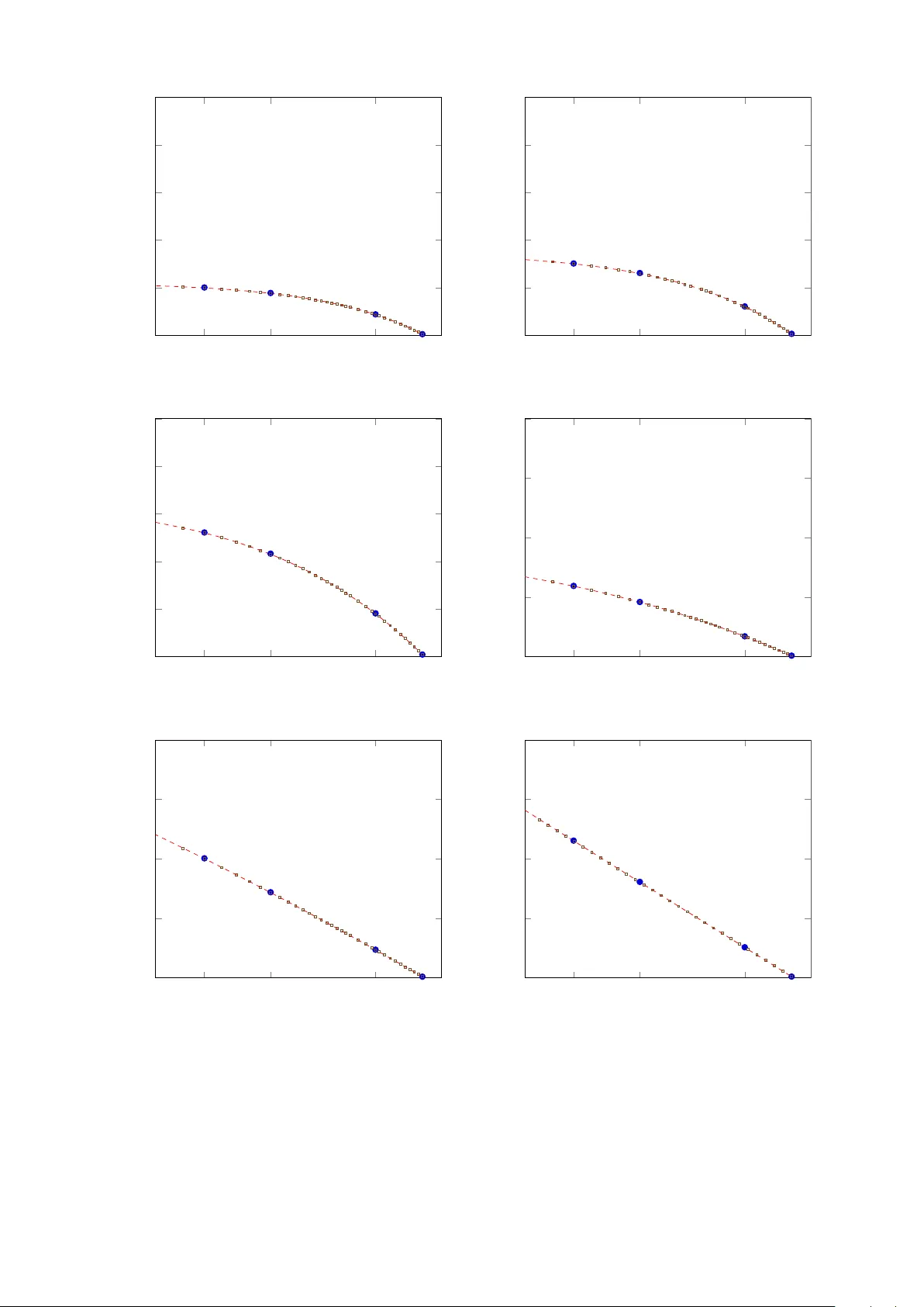
MEAN FIRST ESCAPE TIMES OF BR O WNIAN MOTION ON ASYMPTOTICALL Y HYPERBOLIC AND GAS GIANT METRIC SURF A CES ∗ JESSE GELL-REDMAN † , EMANUEL J ´ OZSEF GODFRIED ‡ , JUSTIN TZOU § , AND LEO TZOU ¶ Abstract. This paper deals with the mean first escape time of Brownian motion on asymptotically hyperb olic and gas giant surfaces. W e show that for a b oundary defining function ρ , the mean first escap e time u ε ( x ) from the truncated Riemannian surface with an asymptotically hyperb olic metric ( M ε , ¯ g /ρ 2 ) = ( { x ∈ M : ρ ( x ) ≥ ε } , ¯ g /ρ 2 ) ⊂ ( M , ¯ g /ρ 2 ) satisfies the asymptotic expansion u ε ( x ) = − log ε + O (1) as ε → 0. F urthermore, we show that in the case of a gas giant metric g = ¯ g /ρ α , where α ∈ (0 , 2), the mean first escap e time from the surface ( M ε , ¯ g /ρ α ) satisfies u ε ( x ) = O (1) as ε → 0. Using techniques from the theory of p olyhomogeneous conormal functions w e explain this difference betw een in the mean first escap e time on gas giant metric surfaces and asymptotically hyperb olic surfaces on the unit disc. Finally , we confirm these results using Monte Carlo simulations and finite difference metho ds on the disc. Key w ords. Hyp erb olic Brownian motion, Narrow escap e problem MSC co des. Primary: 58J65, Secondary: 58J32, 58J40, 60J65, 92C37 1. In tro duction. W e study narro w escape problems for Brownian motion on asymptotically hy- p erb olic surfaces M , equipp ed with a conformally compact metric g = ¯ g /ρ 2 , where ρ is a b oundary defining function and ¯ g is a smooth, non-degenerate Riemannian metric. In this setting, the narrow escap e problem concerns the first time τ x ε a Brownian particle X x t , starting at a p oint x ∈ M , escap es the region M ε = { x ∈ M : ρ ( x ) ≥ ε } . W e then denote the mean first escape time (MFET) from M ε of the Brownian motion starting at x ∈ M ε b y u ε ( x ) = E [ τ x ε ]. Narro w escap e problems ha ve b een extensiv ely studied in Euclidean and Riemannian settings, moti- v ated in part b y applications in cellular biology , such as in the modelling of the timescales of ion diffusion or protein transport (readers may refer to [ 20 , 32 , 10 , 21 ] and references therein, with more detailed the- ory and applications found in textb o oks such as [ 6 , 7 , 22 ]). F or example, in a tw o-dimensional b ounded Euclidean domain Ω, the exp ected escap e time through a small absorbing trap of radius ε b ehav es as u ε ∼ −| Ω | log ε + O (1), as ε → 0 [ 20 ]. This result and its generalisations hav e led to a rich literature on related problems, including narrow capture and escap e on Riemannian manifolds [ 35 , 4 , 10 , 29 ]. More refined expansions also account for geometric features. F or instance, in the case of a single circular trap in a Euclidean domain of R 3 , the exp ected escap e time satisfies u ε ∼ | Ω | 4 ε  1 − ε π H log ε  + O (1) , where H is the mean curv ature at the centre of the trap [ 36 ]. These expansions ha ve also b e en extended to Riemannian 3-manifolds using microlo cal tec hniques [ 30 ]. These mo dels often assume uniform diffusion, and the timescales are computed as the target or trap decreases in size. Ho wev er, in certain cellular en vironments, the diffusion pro cess may b e influenced by geometric factors or v arying diffusion rates, leading to non-uniform diffusion patterns. In this w ork, we extend the analysis of narro w escap e to t wo-dimensional asymptotically h yp erb olic and gas giant metric manifolds, which can mo del scenarios where the diffusion rate slows do wn near the b oundary or cellular membrane. Sp ecifically , in the case of an asymptotically hyperb olic manifold, the mo del assumes a slo wdo wn of order 1 /ρ 2 , where ρ is the distance from the b oundary . The central ∗ Submitted to the editors on: March 18, 2026 F unding: J. Gell-Redman is partially supp orted by the Australian Research Council under grant n umber: DP210102319. E.J. Go dfried is partially supp orted b y the Melbourne Research Scholarship and by Stich ting dr Hen- drik Muller’s V aderlandsch F onds. J. Tzou is partially supp orted by the Australian Research Council under grant num b er: DP220101808. L. Tzou is partially supp orted by the Australian Research Council under grant num b ers: DP220101808 and DP260103195. † School of Mathematics & Statistics, The University of Melbourne, Parkville, VIC, 3010, Australia ( j.gell@unimelb.edu.au ) ‡ School of Mathematics & Statistics, The Universit y of Melb ourne, Parkville, VIC, 3010, Australia ( ego d- fried@student.unimelb.edu.au ) § School of Mathematics & Statistics, The Univ ersity of New South W ales, Kensington, NSW, 2033, Australia ( tzou.justin@gmail.com ) ¶ School of Mathematics & Statistics, The Universit y of Melb ourne, Parkville, VIC, 3010, Australia ( leo.tzou@gmail.com ) 1 question we address is: What is the mean first escape time u ε ( x ) of a Bro wnian motion starting at x from M ε , as ε → 0? Prior w ork on Bro wnian motion on h yp erb olic spaces has largely b een probabilistic and restricted to upper half-space mo dels H d with [ 16 ] b eing (one of ) the first articles on h yp erb olic Bro wnian motion, where the authors show “. . . ho w, with the help of Lobach evsky geometry one can obtain a precise solution of the radio-engineering problem of a statistically inhomogeneous w a veguide – of a wa v eguide (transmission line) with random inhomogeneities.” Similarly , in [ 11 ], the authors show “ho w the one- dimensional, classical diffusion of a particle in a quenched random potential . . . is directly related to Bro wnian motion on the hyperb olic plane.” In [ 18 ], the author calculates directly from the Laplace- Beltrami operator the transition probability density , which is then used in pap ers suc h as [ 25 , 13 ] to obtain large time probability densit y distributions of the Brownian motion. Using similar strategies, the hitting probabilities and exponential deca y laws of the h yp erb olic Brown- ian motion on the upp er half-plane H d ha ve b een found [ 9 , 8 ], and in [ 34 ], the author gives the escap e rate of the hyperb olic Brownian motion. Our approach on the other hand builds on metho ds developed in [ 2 ] and expanded in articles such as [ 30 , 29 ]. This allows for robust computation of the mean escap e time and higher momen ts of the asso ciated distribution. Moreov er, our tec hniques can b e adapted to more general geometries. F or any compact Riemannian surface ( M , ¯ g ) with b oundary ∂ M , we can mak e ( M , g = ¯ g /ρ 2 ) into an asymptot- ically hyperb olic surface. Of this surface, w e can then compute the expansion of the mean first escap e time of the Brownian motion starting at x from the manifold M ε . F urthermore, after proving the mean first escap e time from an asymptotically hyperb olic manifold, w e also consider the mean first escap e time from a gas giant metric manifold . These manifolds, recen tly in tro duced in the context of inv erse problems by [ 12 ], hav e metrics of the form g = ¯ g /ρ α for α ∈ (0 , 2), with the limit as α → 2 b eing the asymptotically h yp erb olic case. This corresp onds to a slo wdown of order 1 /ρ α of the diffusion rate near the b oundary , whic h compared to asymptotically hyperb olic case, is less extreme. Such manifolds exhibit interesting geometric b ehaviour: geo desics reach the b oundary in finite time, while the volume may be finite or infinite dep ending on the dimension and α . Due to the recen t introduction of gas gian t geometries, this paper will, to the authors’ kno wledge, be first treatmen t of Brownian motion and narro w escap e problems in such geometries. 1.1. Notational con v en tions. W e w ork on Riemannian manifolds ( M , g ) with b oundary ∂ M and induced metric h = ι ∗ ∂ M g ∈ S 2 ( ∂ M ). The Laplace-Beltrami operator is giv en in lo cal coordinates x i b y (1.1) ∆ g = 1 p | g | ∂ i  p | g | g ij ∂ j  , whic h has non-p ositive eigenv alues. The normal deriv ative ∂ ν is outw ard p oin ting, so that Green’s form ula is given b y (1.2) Z M (∆ g u ) v − u (∆ g v ) dV ol g = Z ∂ M ( ∂ ν u ) v − u ( ∂ ν v ) dV ol h . 1.2. The statemen t of the problem and theorem. Let ( M , ∂ M , ¯ g ) be a compact connected orien table smo oth non-degenerate Riemannian manifold of dimension tw o. Let ρ ( x ) : M → (0 , ∞ ) be an y b oundary defining function. Then the manifold ( M , ∂ M , g = ¯ g /ρ 2 ) is complete, and the sectional curv atures are −| dρ ( x ) | ¯ g on ∂ M . W e say that ( M , ∂ M ) is a asymptotically h yp erb olic manifold if the sectional curv atures are − 1 on ∂ M . F or ε > 0, let M ε b e the Riemannian manifold with b oundary defined by M ε := { x ∈ M : ρ ( x ) ≥ ε } . (1.3) Set ( X x t , P x ) to be the Brownian motion on ( M , ∂ M , g ) starting at x , and let τ x ε denote the first time that the Brownian motion X x t is outside M ε , i.e. τ x ε := inf { t ≥ 0 : X x t ∈ M \ M ε } . W e wish to study the b ehaviour of the mean first escape time E ( τ x ε ) as ε → 0. In [ 30 , App endix A] it is sho wn that u ε ( x ) := E ( τ x ε ) satisfies the b oundary v alue problem (1.4) ∆ g u ε ( x ) | x ∈ M ◦ ε = − 1 , u ε ( x ) | x ∈ ∂ M ε = 0 for u ε ∈ H 2 ( M ε ) ∩ H 1 0 ( M ε ) . Based on this b oundary v alue problem, we state the main theorem. 2 Theorem 1.1. Assume that u ε ( x ) satisfies the c onditions of Equation ( 1.4 ) , then ther e ar e functions ˜ U ε ( x ) and r ε ( x ) such that (1.5) u ε ( x ) = − log ε + ˜ U ε ( x ) + r ε ( x ) , wher e for e ach fixe d x ∈ M ε the function ˜ U ε ( x ) = O (1) as ε → 0 and for e ach fixe d x ∈ M ε ther e is a p ositive c onstant D x such that | r ε ( x ) | ≤ D x ε log ε as ε → 0 . F urthermor e, if K ⋐ M ◦ is c omp act then, the function ˜ U ε ( x ) c onver ges uniformly to some smo oth b ounde d function ˜ U ( x ) on K and ther e is a p ositive c onstant D K such that sup x ∈ K | r ε ( x ) | ≤ D K ε log ε . 1.3. Outline of the pap er. In section 2 we pro vide some geometric background for our situation of a tw o-dimensional compact connected manifold with b oundary , giv e some information on the Green’s function G ( x ; y ) ∈ D ′ ( M × M ) and provide useful lemmas with references for the rest of the pap er. W e complete the pro of of Theorem 1.1 in section 3 using the information given in section 2 . This pro of is extended in section 4 , where we first provide some additional information on gas giant geometries, and then prov e Theorem 4.1 alluded to in section 1 using techniques from sections 2 and 3 . In section 5 we sho w ho w the limiting case of Theorem 4.1 gives the same results as Theorem 1.1 . Finally , we supplement the theorems in this pap er with Monte Carlo simulations in section 6 . 2. Boundary co ordinates systems and Green’s functions. 2.1. Boundary co ordinate systems. W e begin this discussion on the compact Riemannian man- ifold with b oundary ( M , ∂ M , ¯ g ). F or δ > 0 small we define the manifold M δ b y (2.1) M δ := { x ∈ M : ρ ( x ) > δ } . On M \ M δ w e ha ve the co ordinate system giv en by x 7→ ( ρ ( x ) , θ ( x )), where θ ( x ) ∈ ∂ M is the closest p oin t on the b oundary to x ∈ M \ M δ . Observ e that if v ∈ T (0 ,θ ( x )) M with | v | g = 1 and v ⊥ ¯ g T (0 ,θ ( x )) ∂ M , then x = exp (0 ,θ ( x )) ( ρ ( x ) v ). The metric in this co ordinate systems is thus given b y (2.2) ¯ g = d ρ 2 + ˜ β ( ρ, θ )d θ 2 for some smo oth function ˜ β . Since dim M = 2, all Riemannian metrics are conformally related [ 23 , Chapter 7]. In particular, ¯ g is conformally related to a metric ¯ g 0 , such that ( M \ M δ , ¯ g 0 ) is isometric to the annulus ( D \ D 1 − ¯ δ , g Euc ) with inner radius 1 − ¯ δ and outer radius 1 for some 0 < ¯ δ < 1 under some isomey Φ : M \ M δ → D \ D 1 − ¯ δ , with Φ( ∂ M ) = ∂ D . In particular, since ¯ g and ¯ g 0 are conformally related, there is a smo oth function b ( x ) ∈ C ∞ ( M ) and a p ositive smooth function β ( x ) = e b ( x ) ∈ C ∞ ( M ) such that (2.3) ¯ g = β ( x ) · ¯ g 0 = e − b · ¯ g 0 . Definition 2.1. We define the b oundary defining function ρ 0 = Φ ∗ (  ) ∈ C ∞ ( M \ M δ ) to b e the pul lb ack under the isometric diffe omorphism Φ of the b oundary defining function  ∈ C ∞ ( D \ D 1 − ¯ δ ) given by (2.4)  : D \ D 1 − ¯ δ → R + : ( r , ϑ ) 7→ 1 2 (1 − r 2 ) , wher e ( r, ϑ ) ar e p olar c o or dinates on D . Lemma 2.2. The b oundary defining function  vanishes on the unit cir cle ∂ D = { ( r , ϑ ) : r = 1 } . F urthermor e, the Riemannian manifold ( D \ D 1 − ¯ δ , g Euc / 2 ) has c onstant sc alar curvatur e of − 2 . Pr o of. The first statement of the lemma follows directly from the definition of  . F or the second statemen t, we compute the scalar curv ature of conformally related surfaces using [ 23 , Theorem 7.30]. W e hav e (2.5) R g Euc /ϱ 2 = e 2 log ϱ ( R g Euc + 2∆ g Euc log  ) =  2  0 − 2  2  = − 2 since the scalar curv ature R g Euc = 0. Lemma 2.3. The metric g Euc on D \ D 1 − ¯ δ c an b e expr esse d as (2.6) g Euc = d x 2 + d y 2 = d r 2 + r 2 d ϑ 2 = 1 1 − 2  d  2 + (1 − 2  )d ϑ 2 = ∞ X n =0 (2  ) n ! d  2 + (1 − 2  )d ϑ 2 . 3 Pr o of. The first equality giv es the Euclidean metric in p olar co ordinates. The second equality then follo ws b y the chain rule for differentiation. The final equation follows b y the geometric series, since the image of  is con tained in the in terv al [0 , ¯ δ − 1 2 ¯ δ 2 ] ⊂ [0 , 1 − δ ′ ) for some δ ′ > 0 for sufficiently small ¯ δ . R emark 2.4. The manifold ( D \ D 1 − ¯ δ , g Euc / 2 ) will b e our mo del manifold throughout this pap er. W e can explicitly compute on this manifold, and using the isome tric diffeomorphism Φ, we can therefore compute on M \ M δ . Lemma 2.5. Ne ar the b oundary ¯ g 0 has the form (2.7) ¯ g 0 = (1 + 2 ρ 0 + O ( ρ 2 0 ))d ρ 2 0 + (1 − 2 ρ 0 )d θ 2 , wher e ρ 0 is the b oundary defining function fr om Definition 2.1 . Pr o of. Since Φ( ∂ M ) = ∂ D , the pullbac k Φ ∗ (d ϑ 2 ) of part of the metric g Euc tangen t to the b oundary ∂ D remains tangent to the pullbac k Φ ∗ ∂ D = ∂ M of the boundary under the isometric diffeomorphism Φ. Hence, w e hav e (2.8) ¯ g 0 = Φ ∗ g Euc = Φ ∗  1 1 − 2  d  2 + (1 − 2  )d ϑ 2  = (1 + 2 ρ 0 + O ( ρ 2 0 ))d ρ 2 0 + (1 − 2 ρ 0 )d θ 2 . Lemma 2.6. Ther e is a p ositive function c ( θ ) ∈ C ∞ ( ∂ M ) such that ne ar the b oundary ∂ M , the b oundary defining functions ar e r elate d by (2.9) ρ 0 = c ( θ ) ρ + O ( ρ 2 ) . F urthermor e, the factor c 2 ( θ ) β (0 , θ ) = 1 for e ach p oint on ∂ M . Pr o of. F rom the local description of the metrics ¯ g in (2.2) , and ¯ g 0 in Lemma 2.5 near the b oundary ∂ M , it follows that the v ector fields ∂ ρ | ρ = ρ 0 =0 := ∂ ∂ ρ     ρ = ρ 0 =0 and ∂ ρ 0 | ρ = ρ 0 =0 := ∂ ∂ ρ 0     ρ = ρ 0 =0 are b oth p erp endicular to the b oundary ∂ M . Hence, since at ev ery p oin t the smo oth vector fields are co-linear, it follows that there is a non-zero smo oth function c ( θ ) ∈ C ∞ ( ∂ M ) such that ∂ ρ 0 = c ( θ ) ∂ ρ for ev ery p oint on the boundary ∂ M . Positivit y follo ws from the fact that b oth smo oth v ector fields are in ward pointing. Restricted to the b oundary ∂ M , from the lo cal descriptions we ha ve 1 = | ∂ ρ | ¯ g = | ∂ ρ 0 | ¯ g 0 . Th us we no w compute restricted to the b oundary ∂ M , 1 = | ∂ ρ 0 | ¯ g 0 = | c ( θ ) ∂ ρ | ¯ g 0 = c ( θ ) β (0 , θ ) 1 / 2 | ∂ ρ | ¯ g = c ( θ ) β (0 , θ ) 1 / 2 , from which c 2 ( θ ) β (0 , θ ) = 1 follows. Hence, the b oundary v alue problem ( 1.4 ) simplifies to (2.10) ∆ ¯ g 0 u ε = − c 2 β ( ρ 0 , θ ) ρ 2 0 = − 1 + β (1) ( θ ) ρ 0 + β (2) ( ρ 0 , θ ) ρ 2 0 . 2.2. Green’s functions. In this subsection w e pro vide, for the metric ¯ g 0 , the Green’s functions, and give a decomposition in to a principal and remainder parts near the b oundary ∂ M . There is a unique Green’s Dirichlet function G 0 ( x ; y ) ∈ D ′ ( M × M ) with the properties [ 3 , Theorem 4.17] (2.11)          ∆ ¯ g 0 ,y G 0 ( x ; y ) = δ x ( y ) for x, y ∈ M ◦ G 0 ( x ; y ) | y ∈ ∂ M = 0 G 0 ( x ; y ) ∈ R for x, y ∈ M G 0 ( x ; y ) = G 0 ( y ; x ) . Since a wa y from the diagonal diag ( M × M ) the Green’s function G 0 ( x ; y ) is smo oth, w e ha ve the follo wing lemma. 4 Lemma 2.7. F or e ach fixe d x 0 ∈ M ◦ , ther e is a p ositive c onstant C x 0 such that (2.12) | G 0 ( x 0 ; y ) | ≤ C x 0 ρ 0 ( y ) for y ∈ M ◦ such that ρ 0 ( y ) ≪ ρ 0 ( x 0 ) . Mor e over, for any K ⋐ M ◦ c omp act, ther e is a p ositive c onstant C K such that (2.13) | G 0 ( x ; y ) | ≤ C K ρ 0 ( y ) for x ∈ K, y ∈ M ◦ with ρ 0 ( y ) ≪ min x ∈ K ρ 0 ( x ) . Pr o of. F or eac h fixed x 0 ∈ M ◦ and y ∈ ∂ M we ha ve (2.14) G 0 ( x 0 , y ) | y ∈ ∂ M = 0 . No w, b ecause G 0 ( x 0 ; y ) is smo oth for eac h fixed x 0 ∈ M ◦ and y ∈ ∂ M , b y applying T a ylor’s theorem in its integral from to the function G 0 ( x 0 ; · ), it follows that at y = ( ρ 0 ( y ) , θ ( y )) G 0 ( x 0 ; y ) = ρ 0 ( y ) Z 1 0 ∂ G 0 ( x 0 ; tρ 0 ( y ) , θ ( y )) ∂ ρ 0 ( y ) d t . Hence, there is a p ositive constan t C x 0 suc h that | G 0 ( x 0 ; y ) | ≤ C x 0 ρ 0 ( y ) for y ∈ M ◦ suc h that ρ 0 ( y ) ≪ ρ 0 ( x 0 ). If K ⋐ M ◦ is compact, we can tak e C K = max x ∈ K C x , then | G 0 ( x ; y ) | ≤ C K ρ 0 ( y ) for x ∈ K, y ∈ M ◦ with ρ 0 ( y ) ≪ min x ∈ K ρ 0 ( x ). W e will now give a decomposition of the Green’s function G 0 ( x ; y ) into a sum of a princip al Gr e en ’s function G 0 , prin ( x ; y ) and r emainder Gr e en ’s function G 0 , rem ( x ; y ). Definition 2.8. Assume without loss of gener ality that ( M \ M δ , ¯ g 0 ) c an b e extende d to some man- ifold ( f M \ M δ , ¯ g 0 ) isometric to ( R 2 \ D 1 − ¯ δ , g Euc ) , and let Φ : f M \ M δ → R 2 \ D 1 − ¯ δ b e this isometry. F or x, y ∈ M \ M δ denote (2.15) | x | := | Φ( x ) | , | x − y | := | Φ( x ) − Φ( y ) | , and x | x | 2 := Φ − 1  Φ( x ) | Φ( x ) | 2  ∈ f M \ M δ , then define the distribution G 0 , prin ( x ; y ) ∈ D ′ ( M × M ) by (2.16) G 0 , prin ( x ; y ) = κ ( x ; y ) 2 π  log | x − y | − log     | x | ·  y − x | x | 2       , wher e κ ( x ; y ) = κ 1 ( x ) · κ 1 ( y ) · κ 0 ( x ; y ) and κ 1 ∈ C ∞ ( M ) , κ 0 ( x ; y ) ∈ C ∞ ( M × M ) ar e smo oth cutoff functions on M with the pr op erties that (2.17) ( κ 1 ( x ) ≡ 1 if ρ 0 ( x ) ≤ δ / 4 κ 1 ( x ) ≡ 0 if ρ 0 ( x ) ≥ δ / 3 and      κ 0 ( x ; y ) ≡ 1 if d ¯ g 0 ( x ; y ) < δ / 4 κ 0 ( x ; y ) ≡ 0 if d ¯ g 0 ( x ; y ) > δ / 3 κ 0 ( x ; y ) ≡ κ 0 ( y ; x ) for al l x, y ∈ M . R emark 2.9. The distribution (2.18) G 0 , prin , A ( z 1 ; z 2 ) = 1 2 π  log | z 1 − z 2 | − log     | z 1 | ·  z 2 − z 1 | z 1 | 2       is the symmetric Green’s function on the unit disc, with the properties of ( 2.11 ) for the Euclidean metric g Euc [ 14 , Section 2.2 Equation (41)]. W e therefore hav e      ∆ g Euc ,z 2 G 0 , prin , A ( z 1 , z 2 ) = δ z 1 ( z 2 ) , G 0 , prin , A ( z 1 , z 2 ) = G 0 , prin , A ( z 2 , z 1 ) , G 0 , prin , A ( z 1 , z 2 ) | | z 2 | =1 = 0 . (2.19) 5 Lemma 2.10. We c an write (2.20) G 0 , prin ( x ; y ) = κ ( x ; y )(Φ ∗ G 0 , prin , A )( x ; y ) = κ ( x ; y ) G 0 , prin , A (Φ( x ); Φ( y )) . Pr o of. In Definition 2.8 , G 0 , prin is exactly defined using the distribution G 0 , prin , A . Lemma 2.11. The distribution G 0 , prin ( x ; y ) is symmetric, i.e. G 0 , prin ( y ; x ) = G 0 , prin ( x ; y ) . Pr o of. The smo oth cut-off function κ ( x ; y ) is symmetric b y definition. On supp κ ( x ; y ) we therefore ha ve G 0 , prin ( y ; x ) = κ ( y ; x ) G 0 , prin , A (Φ( y ); Φ( x )) = κ ( x ; y ) G 0 , prin , A (Φ( x ); Φ( y )) = G 0 , prin ( x ; y ) . (2.21) Proposition 2.12. We have the fol lowing de c omp osition of the Gr e en ’s function G 0 ( x ; y ) (2.22) G 0 ( x ; y ) = G 0 , prin ( x ; y ) + G 0 , rem ( x ; y ) , wher e G 0 , rem ( x ; y ) satisfies 1. G 0 , rem ( x ; y ) is a smo oth symmetric function for x, y ∈ M \ M δ / 4 , satisfying G 0 , rem ( x ; y ) = 0 whenever y ∈ ∂ M , and 2. if 0 < ε ≪ δ , then ther e ther e ar e c onstants C 0 , C 1 , C 2 such that sup z ∈ ∂ M ε | ∂ ν z G 0 , rem ( z ; y ) | ≤ C 0 · ρ 0 ( y ) + C 1 ( ε + ρ ( y )) 2 + C 2 ( ε + ρ ( y )) 3 holds for al l y ∈ M \ M δ / 4 and ε > 0 . Pr o of. W e ha v e ∆ ¯ g 0 ,y G 0 , prin ( x ; y ) = 1 2 π  κ ( x ; y )∆ ¯ g 0 ,y  log | x − y | − log     | x | ·  y − x | x | 2       + F ( x ; y )  . (2.23) Where F ( x ; y ) := ∆ ¯ g 0 ,y κ ( x ; y )  log | x − y | − log     | x | ·  y − x | x | 2       + 2  d y κ ( x ; y ) , d y  log | x − y | − log     | x | ·  y − x | x | 2       ¯ g 0 . (2.24) By Lemma 2.10 , it follo ws that κ ( x ; y ) 2 π ∆ ¯ g 0 ,y  log | x − y | − log     | x | ·  y − x | x | 2       = κ ( x ; y )∆ Φ ∗ g Euc (Φ ∗ G 0 , prin , A )( x ; y ) = κ ( x ; y )Φ ∗ (∆ g Euc G 0 , prin , A )( x ; y ) = κ ( x ; y ) δ x ( y ) , (2.25) since we assumed that ¯ g 0 is isometric to g Euc . So ( 2.23 ) b ecomes ∆ ¯ g 0 ,y G 0 , prin ( x ; y ) = κ ( x ; y ) δ x ( y ) + F ( x ; y ) . (2.26) By construction, we ha ve that the supp orts of d y κ ( x ; y ) and ∆ ¯ g 0 κ ( x ; y ) are contained in the union (2.27) supp d y κ ( x ; y ) , supp ∆ ¯ g 0 ,y κ ( x ; y ) ⊂ ( M δ / 4 \ M δ / 2 ) × ( M δ / 4 \ M δ / 2 ) ∪ { δ / 4 < d ¯ g 0 ( x ; y ) < δ / 2 } . So we ha ve that F ( x ; y ) is smo oth for x, y ∈ M \ M δ / 4 . If w e now let (2.28) G 0 , rem ( x ; y ) := G 0 ( x ; y ) − G 0 , prin ( x ; y ) then for x, y ∈ M \ M δ / 4 w e hav e that ( 2.26 ) b ecomes (2.29) ∆ ¯ g 0 ,y G 0 , rem ( x ; y ) = δ x ( y ) − κ ( x ; y ) δ x ( y ) − F ( x ; y ) = − F ( x ; y ) , since κ ( x ; y ) ≡ 1 for x, y ∈ M \ M δ / 4 . By elliptic regularity [ 37 ], it therefore follows that G 0 , rem ( x ; y ) is smo oth on M \ M δ / 4 . F urthermore, since b oth G 0 ( x ; y ) and G 0 , prin ( x ; y ) are symmetric and zero on the b oundary ∂ M , it follows that G 0 , rem ( y ; x ) = G 0 , rem ( x ; y ) and G ( x ; y ) | y ∈ ∂ M = 0. This concludes Item 1 . 6 Finally , since G 0 , rem ( x ; y ) is jointly smooth near the boundary we can tak e a joint T a ylor p olynomial around ρ 0 ( x ) = ρ 0 ( y ) = 0, such that there are smo oth functions A ij ( θ ( x ) , θ ( y )) such that G 0 , rem ( x ; y ) = A 00 ( θ ( x ) , θ ( y )) + A 10 ( θ ( x ) , θ ( y )) ρ 0 ( x ) + A 01 ( θ ( x ) , θ ( y )) ρ 0 ( y ) + A 11 ( θ ( x ) , θ ( y )) ρ 0 ( x ) ρ 0 ( y ) + A 20 ( θ ( x ) , θ ( y )) ρ 0 ( x ) 2 + A 02 ( θ ( x ) , θ ( y )) ρ 0 ( y ) 2 + R 3 ( x ; y ) (2.30) with the remainder R 3 ( x ; y ) given b y R 3 ( x ; y ) = X i + j =3 3( ρ 0 ( x )) i ( ρ 0 ( y )) j i ! j ! Z 1 0 (1 − t ) 2 ∂ 3 G 0 , rem ( tρ 0 ( x ) , θ ( x ) , tρ 0 ( y ) , θ ( y )) ( ∂ ρ 0 ( x )) i ( ∂ ρ 0 ( y )) j d t (2.31) Since G 0 , rem ( x ; y ) | y ∈ ∂ M ≡ 0, it follows that the functions A 00 , A 10 are iden tically 0. F urthermore, also b ecause G 0 , rem ( x ; y ) | y ∈ ∂ M ≡ 0 for all x ∈ M ◦ , w e find that ∂ ν z G 0 , rem ( z ; y ) | y ∈ ∂ M z ∈ ∂ M ε ≡ 0, and that the functions A 10 = A 20 are identically 0 . Then, since the normal deriv ative ∂ ν at the boundary ∂ M ε in the local co ordinates ( ρ 0 , θ ) satisfy the relation ∂ ν = − ∂ ρ 0 | ρ 0 = ε , we find that (2.32) ∂ ν z G 0 , rem ( z ; y ) | z ∈ ∂ M ε = − A 11 ( θ ( z ) , θ ( y )) ρ 0 ( y ) + ∂ ν z R 3 ( z ; y ) | z ∈ ∂ M ε . W e can no w b ound the function A 11 ( θ ( x ) , θ ( y )) uniformly on ∂ M × ∂ M by a constan t C 0 > 0 such that sup θ ( x ) ,θ ( y ) ∈ ∂ M | A 11 ( θ ( x ) , θ ( y )) | ≤ C 0 . F urthermore,     ∂ ν z R 3 ( z ; y ) | z ∈ ∂ M ε     ≤ X i + j =3     3 i ( ε ) i − 1 ( ρ 0 ( y )) j i ! j ! Z 1 0 (1 − t ) 2 ∂ 3 G 0 , rem ( tε, θ ( z ) , tρ 0 ( y ) , θ ( y )) ( ∂ ρ 0 ( x )) i ( ∂ ρ 0 ( y )) j d t     + X i + j =3     3( ε ) i ( ρ 0 ( y )) j i ! j ! Z 1 0 (1 − t ) 2 ∂ 4 G 0 , rem ( tε, θ ( z ) , tρ 0 ( y ) , θ ( y )) ( ∂ ρ 0 ( x )) i +1 ( ∂ ρ 0 ( y )) j d t     ≤ C 1 ( ε + ρ ( y )) 2 + C 2 ( ε + ρ ( y )) 3 b y bounding the deriv atives uniformly on the righ t hand side o ver M \ M δ / 4 × M \ M δ / 4 due to the joint smo othness of the function G 0 , rem ( x ; y ). Then, it follows that there are constants C 0 , C 1 , C 2 suc h that sup z ∈ ∂ M ε | ∂ ν z G 0 , rem ( z ; y ) | ≤ C 0 · ρ 0 ( y ) + C 1 ( ε + ρ ( y )) 2 + C 2 ( ε + ρ ( y )) 3 holds for all y ∈ M \ M δ / 4 and ε > 0. This concludes Item 2 . In section 3 we will use these decomp ositions to explicitly compute some integrals near the b oundary . 2.3. Sob olev spaces. In this subsection we giv e definitions of the Sobolev spaces of in terest in this pap er. Definition 2.13. F or k ∈ Z + , (Ω , ¯ g ) ⊂ ( M , ¯ g ) an op en domain and ¯ g a smo oth metric on Ω , we define the Sob olev sp ac es as the c ompletions with r esp e ct to the H k (Ω , ¯ g ) -norm H k (Ω , ¯ g ) := { u ∈ C ∞ (Ω) } ∥·∥ H k (Ω , ¯ g ) H k,p 0 (Ω , ¯ g ) := { u ∈ C ∞ 0 (Ω) } ∥·∥ H k (Ω , ¯ g ) , (2.33) wher e the H k (Ω , ¯ g ) norm is given by ∥ f ∥ H k (Ω , ¯ g ) = k X i =0 ∥ D i f ∥ 2 L 2 (Ω , ¯ g ) ! 1 / 2 wher e we interpr et the D i f as the i th we ak derivative of f ∈ C ∞ (Ω) . 7 We define the lo c alise d Sob olev sp ac e (2.34) H k loc (Ω , ¯ g ) := { u ∈ D ′ (Ω) : ϕu ∈ H k (Ω , ¯ g ) for al l ϕ ∈ C ∞ 0 (Ω) } . F or k ∈ Z + , the sp ac e H − k (Ω , ¯ g ) is define d as the formal dual to H k 0 (Ω , ¯ g ) . F or non-inte ger values l > 0 , we define the Sob olev sp ac es H l (Ω , ¯ g ) using the c omplex interp olation metho d [ 5 , The or em 6.4.5 p art (7)]. This definition depends implicitly on the metric (and therefore also on the L 2 -norms). By [ 19 , Proposition 2.2], it follo ws that if ¯ g , ¯ h are tw o smo oth metrics for Ω, then the Sob olev spaces H l (Ω , ¯ g ) = H l (Ω , ¯ h ), since the metrics ¯ g , and ¯ h provide equiv alen t norms on Ω. Next, the Poincar ´ e inequality also provides an equiv alent norm for H 1 0 (Ω , ¯ g ). Indeed, w e see for ϕ ∈ H 1 0 (Ω , ¯ g ) that (2.35) ∥ Dϕ ∥ L 2 (Ω , ¯ g ) ≤  ∥ ϕ ∥ 2 L 2 (Ω , ¯ g ) + ∥ D ϕ ∥ 2 L 2 (Ω , ¯ g )  1 / 2 ≤ C (Ω) ∥ D ϕ ∥ L 2 (Ω , ¯ g ) . The second inequalit y is the P oincar´ e inequality . Since ∥ ϕ ∥ H 1 (Ω , ¯ g ) := ( ∥ ϕ ∥ 2 L 2 (Ω , ¯ g ) + ∥ Dϕ ∥ 2 L 2 (Ω , ¯ g ) ) 1 / 2 the conclusion follows. The follo wing lemmas sho w that (w eak) solutions to elliptic b oundary v alue problems hav e the “exp ected” regularity . Proposition 2.14. L et Ω ⊂ M a b ounde d domain with smo oth b oundary and let ¯ g b e a smo oth metric on Ω , then if f ∈ H − 1 (Ω , ¯ g ) , the b oundary value pr oblem (2.36) ( ∆ ¯ g u = f u | ∂ Ω = 0 has a unique solution u ∈ H 1 0 (Ω , ¯ g ) and ther e is a c onstant C > 0 such that (2.37) ∥ u ∥ H 1 (Ω , ¯ g ) ≤ C ∥ f ∥ H − 1 (Ω , ¯ g ) This is a consequence of the b oundary elliptic regularit y [ 26 , Theorem 4.10] together with the maxim um principle for the Laplacian. Proposition 2.15. L et Ω ⊂ M a b ounde d domain with smo oth b oundary, then for and s ∈ R , if f ∈ H s − 2 loc (Ω , ¯ g ) , and if u satisfies ∆ ¯ g u = f for x ∈ Ω , then u ∈ H s loc (Ω , ¯ g ) . This is [ 15 , Theorem 6.33] for smo oth manifolds. Proposition 2.16 (Sob olev embedding theorem). L et M b e a c omp act smo oth Riemannian man- ifold of dimension n with smo oth b oundary ∂ M , then the emb e dding H l ( M , ¯ g )  → C s ( M ) is c ontinuous if l − n/ 2 > s ≥ 0 for inte ger s . F or a pro of see e.g. [ 3 , Theorem 2.30]. W e finish this section with Hardy’s inequalit y . F or a discussion of the b est constants see [ 24 ]. Proposition 2.17. L et Ω ⊂ M b e an op en domain and let ¯ g b e a smo oth metric on Ω , then ther e exists a c onstant c such that for u ∈ H 1 0 (Ω , ¯ g ) the ine quality (2.38) Z Ω  | u ( x ) | dist ¯ g ( x, ∂ Ω)  2 dV ol ¯ g ( x ) ≤ c Z Ω | D u | 2 dV ol ¯ g ( x ) holds. 3. Pro of of Theorem 1.1 . Now to con tinue, assume that ε is sufficiently small. Fix some x 0 ∈ M ◦ ε and let δ > ε > 0 such that ρ 0 ( x 0 ) > δ . Similarly to b efore, set M δ = { x ∈ M : ρ 0 ( x ) ≥ δ } . W e further assume that the the estimates from Lemma 2.7 hold for y ∈ M \ M δ . This can b e achiev ed b y choosing δ sufficiently small. On the neighbourho o d M ε \ M δ w e can define the function (3.1) v ε ( x ) = log ρ 0 ( x ) − log ε . On the model asymptotically hyperb olic surface ( D \ D 1 − δ , g Euc / 2 ), the function v ε ( x ) solv es the b ound- ary v alue problem ( 1.4 ) exactly . By m ultiplying v ε with a smo oth cut-off function χ ∈ C ∞ ( M ), depending only on ρ 0 ( x ), which has the prop erties χ | ρ 0 ( x ) <δ / 2 ≡ 1 and supp χ ⊂ M \ M δ , we see that the function χv ε ∈ C ∞ ( M ε ). 8 Proposition 3.1. F or x ∈ M ε , let w ε : M ε → R with w ε ( x ) = u ε ( x ) − χ ( x ) v ε ( x ) wher e u ε is the solution to ( 1.4 ) . Then 1. Ther e ar e smo oth functions f 1 , f 2 ∈ C ∞ ( M ε ) such that (3.2) ∆ ¯ g 0 w ε ( x ) = f 1 ( x ) log ε + f 2 ( x ) on M ε . 2. The function f 1 extends to a smo oth function on M which is 0 on M \ M ε . The inte gr al I 1 ( x ) = Z M ε G 0 ( x ; y ) f 1 ( y ) dV ol ¯ g 0 ( y ) = χ ( x ) − 1 . (3.3) 3. F or e ach fixe d x 0 = ( ρ 0 ( x 0 ) , θ ( x 0 )) ∈ M ◦ , the function f 2 ( ρ 0 , θ ) = − (1 − χ ) + β (1) ( θ ) ρ 0 + β (2) ( ρ 0 , θ ) ρ 2 0 − ∆ ¯ g 0 χ · log ρ 0 − 2 ⟨ dχ, dv ε ⟩ ¯ g 0 (3.4) satisfies I 2 ( x 0 ) = Z M ε G 0 ( x 0 ; y ) f 2 ( y ) dV ol ¯ g 0 ( y ) = O (1) , (3.5) as ε → 0 . 4. Final ly, if K ⋐ M ◦ is c omp act, the function ˜ u ε ( x ) := I 2 ( x ) c onver ges uniformly on K to some b ounde d smo oth function ˜ u ( x ) ∈ C ∞ ( K ) given by (3.6) ˜ u ( x ) := Z M G 0 ( x ; y ) f 2 ( y ) dV ol ¯ g 0 ( y ) . Pr o of. W e simply calculate the Laplacian applied to w ε and use expression ( 3.1 ) for v ε to get ∆ ¯ g 0 w ε ( x ) = − 1 − χ ( x ) + β (1) ( θ ) ρ 0 ( x ) + β (2) ( ρ 0 , θ ) ρ 0 ( x ) 2 − ∆ ¯ g 0 ( χ ( x )) v ε ( x ) − 2 ⟨ dχ ( x ) , dv ε ( x ) ⟩ ¯ g 0 = f 1 ( x ) log ε + f 2 ( x ) , (3.7) where f 1 = ∆ ¯ g 0 χ and f 2 = − (1 − χ ) + β (1) ( θ ) ρ 0 + β (2) ( ρ 0 , θ ) ρ 2 0 − ∆ ¯ g 0 χ · log ρ 0 − 2 ⟨ dχ, dv ε ⟩ ¯ g 0 . Then by construction f 1 , f 2 ∈ C ∞ ( M ε ) are smo oth. This gives part 1. No w, w e note that f 1 is identically 0 on a neigh b ourho o d of the b oundary ∂ M ε , so that w e can extend f 1 to a smo oth function on M with f 1 | M \ M ε ≡ 0. Giv en these expressions we can compute I 1 ( x ) = Z M ε G 0 ( x ; y ) f 1 ( y ) dV ol ¯ g 0 ( x ) = Z M ε G 0 ( x ; y )∆ ¯ g 0 χ ( y ) dV ol ¯ g 0 ( y ) = χ ( x ) + Z ∂ M ε G 0 ( x ; y ) ∂ ν χ ( y ) − ∂ ν y G 0 ( x ; y ) χ ( y ) dV ol h ( y ) = χ ( x ) − 1 , (3.8) due to fact that R ∂ M ε ∂ ν G 0 ( x ; y ) dV ol h ( y ) = 1 by in tegration by parts, and hence I 1 ( x ) ∈ C ∞ ( M ). This giv es part 2. W e now sho w that for each x 0 ∈ M ◦ the integral I 2 ( x 0 ) is O (1) as ε → 0. The functions − 1 − χ ρ 2 0 , ∆ ¯ g 0 χ · log ρ 0 , ⟨ dχ, dv ε ⟩ ¯ g 0 are all identically 0 in a collar neighbourho o d containing ∂ M ε of the b oundary ∂ M . Similarly , the function β (2) ( ρ 0 , θ ) /ρ 2 0 is a bounded smo oth function on this collar neighbourho o d. Hence, for each x 0 ∈ M ε the function G 0 ( x 0 ; y )  − 1 − χ + β (2) ( ρ 0 , θ ) ρ 2 0 − ∆ ¯ g 0 χ · log ρ 0 − ⟨ dχ, dv ε ⟩ ¯ g 0  9 is absolutely integrable ov er M . Finally , b y Lemma 2.7 we notice that for e ac h x 0 ∈ M ◦ the function G 0 ( x 0 ; y ) /ρ 0 ( y ) is also absolutely integrable o ver M . Then, the integral Z M ε G 0 ( x ; y ) f 2 ( y ) dV ol ¯ g 0 ( y ) = Z M G 0 ( x ; y ) f 2 ( y ) 1 ρ 0 >ε ( y ) dV ol ¯ g 0 ( y ) con verges to Z M G 0 ( x ; y ) f 2 ( y ) dV ol ¯ g 0 ( y ) = O (1) , b y the dominated conv ergence theorem. This giv es part 3. W e can extend the smooth function f 2 to a distribution in the Sob olev space H − 1 ( M , ¯ g 0 ) b y setting for each ϕ ∈ H 1 0 ( M , ¯ g 0 ), the pairing (3.9) ⟨ ϕ, f 2 ⟩ = Z M ϕ ( x )  − (1 − χ ) + β (1) ( θ ) ρ 0 + β (2) ( ρ 0 , θ ) ρ 2 0 − ∆ ¯ g 0 χ · log ρ 0 − 2 ⟨ dχ, dv ε ⟩ ¯ g 0  dV ol ¯ g 0 ( x ) . Note that ϕ 7→ ⟨ ϕ, f 2 ⟩ is a b ounded linear function on H 1 0 ( M , ¯ g 0 ) thanks to Hardy’s inequality , Proposi- tion 2.17 . Giv en this, we observ e then, that the function ˜ u ε ( x ) : M → R defined by (3.10) ˜ u ε ( x ) = I 2 ( x ) = Z M ε G 0 ( x ; y ) f 2 ( y ) dV ol ¯ g 0 ( y ) = Z M G 0 ( x ; y ) 1 ρ 0 >ε ( y ) f 2 dV ol ¯ g 0 ( y ) solv es the partial differential equation (3.11) ( ∆ ¯ g 0 ˜ u ε ( x ) = 1 ρ 0 >ε ( x ) f 2 ( x ) for x ∈ M ◦ ˜ u ε | ∂ M = 0 . F or any ε > 0, Prop osition 2.14 implies that the function ˜ u ε ( x ) ∈ H 1 0 ( M , ¯ g 0 ), since the right hand side 1 ρ 0 >ε f 2 ∈ H − 1 ( M , ¯ g 0 ). Notice further that ˜ u ( x ) giv en by ( 3.6 ) solves the distributional partial differential equation (3.12) ( ∆ ¯ g 0 ˜ u ( x ) = f 2 ( x ) for x ∈ M ◦ ˜ u | ∂ M = 0 W e now show that ˜ u ε ( x ) conv erges to ˜ u ( x ) in H 1 0 ( M , ¯ g 0 ). By Proposition 2.14 it follows that solutions to (3.12) are unique. This shows that ˜ u ( x ) ∈ H 1 0 ( M , ¯ g 0 ) is the unique solution to (3.12) . No w we hav e b y the Cauch y-Sch wartz inequalit y and by Prop osition 2.17 , for each ε > 0 and all ϕ ∈ H 1 0 ( M , ¯ g 0 ) that there are constan ts c, d, d ′ > 0 such that Z M | ( 1 ρ 0 >ε ( x ) − 1) f 2 ( x ) ϕ ( x ) | dV ol ¯ g 0 x ≤ c Z M     ϕ ρ 0     2 dV ol ¯ g 0 ( x ) ! 1 / 2 ∥ 1 ρ 0 >ε − 1 ∥ L 2 ( M , ¯ g 0 ) ≤ d  Z M | D ϕ ( x ) | 2 dV ol ¯ g 0 x  1 / 2 · ∥ 1 ρ 0 >ε − 1 ∥ L 2 ( M , ¯ g 0 ) = d ∥ D ϕ ∥ L 2 ( M ) · ∥ 1 ρ 0 >ε − 1 ∥ L 2 ( M , ¯ g 0 ) ≤ d ′ ∥ ϕ ∥ H 1 ( M , ¯ g 0 ) · ∥ 1 ρ 0 >ε − 1 ∥ L 2 ( M , ¯ g 0 ) . (3.13) Hence, we ha ve that in the dual space top ology on H − 1 ( M , ¯ g 0 ), that ∥ ∆ ¯ g 0 ( ˜ u ε − ˜ u ) ∥ H − 1 ( M , ¯ g 0 ) = sup φ ∈ H 1 0 ( M , ¯ g 0 ) ∥ φ ∥ H 1 ( M , ¯ g 0 )=1 | ⟨ ∆ ¯ g 0 ( ˜ u ε − ˜ u ) , ϕ ⟩ | = sup φ ∈ H 1 0 ( M , ¯ g 0 ) ∥ φ ∥ H 1 ( M, ¯ g 0 ) =1 | ⟨ ( 1 ρ 0 >ε ( x ) − 1) f 2 ( x ) , ϕ ⟩ | ≤ d ′ ∥ 1 ρ 0 >ε − 1 ∥ L 2 ( M , ¯ g 0 ) ε → 0 − − − → 0 . (3.14) Th us by Proposition 2.14 , it follows that, there is a constant C such that (3.15) ∥ ˜ u ε − ˜ u ∥ H 1 ( M , ¯ g 0 ) ≤ C ∥ 1 ρ 0 >ε − 1 ∥ L 2 ( M , ¯ g 0 ) ε → 0 − − − → 0 , 10 hence ˜ u ε ( x ) conv erges to ˜ u ( x ) in H 1 0 . No w for any compact set K ⋐ M ◦ , w e can then tak e ε > 0 sufficien tly small, such that the set K ⊂ { ρ 0 > 2 ε } . Because f 2 ∈ H k − 2 loc ( M , ¯ g 0 ) for an y k ∈ Z + , it follows that ˜ u ε , ˜ u ∈ H k loc ( M , ¯ g 0 ) for an y k ∈ Z + b y Prop osition 2.15 . F urthermore, for any ϕ ∈ C ∞ 0 ( M ) such that supp ϕ ⊂ K we ha ve (3.16) ϕ ∆ ¯ g 0 ˜ u ε = ϕf 2 = ϕ ∆ ¯ g 0 ˜ u , which implies that ϕ ∆ ¯ g 0 ( ˜ u ε − ˜ u ) = 0 . This means that ˜ u ε − ˜ u ∈ H k ( K, ¯ g 0 ) for any k ∈ Z + . Now by the complex in terp olation metho d [ 5 , Theorem 6.4.5 part (7)], w e find that for any l = (1 − θ ′ ) k + θ ′ , θ ′ ∈ (0 , 1) ∥ ˜ u ε − ˜ u ∥ H l ( K, ¯ g 0 ) ≤ C ( k ) ∥ ˜ u ε − ˜ u ∥ 1 − θ ′ H k ( K, ¯ g 0 ) · ∥ ˜ u ε − ˜ u ∥ θ ′ H 1 ( K, ¯ g 0 ) ≤ C ( k )( ∥ ˜ u ε ∥ 1 − θ ′ H k ( K, ¯ g 0 ) + ∥ ˜ u ∥ 1 − θ ′ H k ( K, ¯ g 0 ) ) · ∥ ˜ u ε − ˜ u ∥ θ ′ H 1 ( K, ¯ g 0 ) ε → 0 − − − → 0 . (3.17) Hence by Proposition 2.16 it follows that for an y integer s w e can find l sufficiently large such that (3.18) ∥ ˜ u ε − ˜ u ∥ C s ( K ) ≤ C ( s, k ′ ) ∥ ˜ u ε − ˜ u ∥ H l ( M , ¯ g 0 ) ε → 0 − − − → 0 . This shows that for an y compact subsets K ⋐ M ◦ , the function ˜ u ∈ C ∞ ( K ) and ˜ u ε con verges uniformly to ˜ u on K . This finishes the pro of of the prop osition. W e now giv e one more estimate on the functions f 1 and f 2 in the following proposition. Proposition 3.2. L et f 1 , f 2 ∈ C ∞ ( M ε ) b e the functions fr om Pr op osition 3.1 . Then, for z ∈ ∂ M ε , ther e ar e functions g 1 , g 2 : ∂ M ε → R such that (3.19) Z M ε ∂ ν z G 0 ( z ; y )( f 1 ( y ) log ε + f 2 ( y )) dV ol ¯ g 0 ( y ) = g 1 ( z ) log ε + g 2 ( z ) , with sup z ∈ ∂ M ε | g i ( z ) | = O (1) as ε → 0 . Pr o of. Define the family of functions ˜ g 1 , ˜ g 2 : ∂ M ε → R by (3.20) ˜ g 1 ( z ) := Z M ε ∂ ν z G 0 ( z ; y ) f 1 ( y ) dV ol ¯ g 0 ( y ) and (3.21) ˜ g 2 ( z ) := Z M ε ∂ ν z G 0 ( z ; y )  1 − χ ρ 2 0 + ∆ ¯ g 0 χ · log ρ 0 + ⟨ dχ, dv ε ⟩ ¯ g 0  dV ol ¯ g 0 ( y ) . Lemma 3.3. F or ε smal l enough, ˜ g 1 : ∂ M ε → R is c onstant 0 . F urthermor e, the function ˜ g 2 ( z ) satisfies the estimate sup z ∈ ∂ M ε | ˜ g 2 ( z ) | = O (1) as ε → 0 . By Lemma 3.3 we ha ve that the left hand side of ( 3.19 ) b ecomes, for z ∈ ∂ M ε Z M ε ∂ ν z G 0 ( z ; y )( f 1 ( y ) log ε + f 2 ( y )) dV ol ¯ g 0 ( y ) = ˜ g 2 ( z ) + Z M ε ∂ ν z G 0 ( z ; y ) β (1) ( θ ( y )) ρ 0 ( y ) + β (2) ( ρ 0 , θ ) ρ 0 ( y ) 2 dV ol ¯ g 0 ( y ) (3.22) with ˜ g 2 ( z ) uniformly b ounded on ∂ M ε as ε → 0. T o this end, it remains to analyse the integral (3.23) Z M ε ∂ ν z G 0 ( z ; y ) β (1) ( θ ( y )) ρ 0 ( y ) + β (2) ( ρ 0 , θ ) ρ 0 ( y ) 2 dV ol ¯ g 0 ( y ) . W e shall show that the absolute integral is b ounded uniformly b y a function which is a multiple of log ε for ε > 0. W e do this with the following four lemmas. Lemma 3.4. The function (3.24) h 1 ( z ) = Z M δ/ 4 ∂ ν z G 0 ( z ; y ) β (1) ( θ ( y )) ρ 0 ( y ) dV ol ¯ g 0 ( y ) satisfies the estimate sup z ∈ ∂ M ε | h 1 ( z ) | = O (1) as ε → 0 . 11 Lemma 3.5. L et G 0 , prin b e the princip al p art of the Gr e en ’s function fr om Definition 2.8 . Then the function (3.25) h 2 ( z ) = Z M ε \ M δ/ 4 ∂ ν z G 0 , prin ( z ; y ) β (1) ( θ ( y )) ρ 0 ( y ) dV ol ¯ g 0 ( y ) satisfies the estimate sup z ∈ ∂ M ε | h ( z ) | = O ( − log ε ) as ε → 0 . Lemma 3.6. L et G 0 , rem b e the r emainder p art of the Gr e en ’s function fr om Definition 2.8 . Then the function (3.26) h 3 ( z ) = Z M ε \ M δ/ 4 ∂ ν z G 0 , rem ( z ; y ) β (1) ( θ ( y )) ρ 0 ( y ) dV ol ¯ g 0 ( y ) satisfies the estimate sup z ∈ ∂ M ε | h 3 ( z ) | = O (1) as ε → 0 . Lemma 3.7. The function (3.27) h 4 ( z ) = Z M ε ∂ ν z G 0 ( z ; y ) β (2) ( ρ 0 ( y ) , θ ( y )) ρ 0 ( y ) 2 dV ol ¯ g 0 ( y ) satisfies the estimate sup z ∈ ∂ M ε | h 1 ( z ) | = O (1) as ε → 0 . By Lemma 3.5 , it follo ws that sup z ∈ ∂ M ε | h 2 ( z ) | = O (log ε ) as ε → 0, hence the function (3.28) g 1 ( z ) = h 2 ( z ) log ε satisfies sup z ∈ ∂ M ε | g 1 ( z ) | = O (1) as ε → 0. Similarly , Lemma 3.3 sho ws that the function ˜ g 2 ( z ) satisfies the estimate sup z ∈ ∂ M ε | ˜ g 2 ( z ) | = O (1) as ε → 0. Lemma 3.4 sho ws that the function h 1 ( z ) satisfies the estimate sup z ∈ ∂ M ε | h 1 ( z ) | = O (1) as ε → 0, Lemma 3.6 sho ws that the function h 2 ( z ) satisfies the estimate sup z ∈ ∂ M ε | h 3 ( z ) | = O (1) as ε → 0 and Lemma 3.7 shows that the functions h 3 ( z ) satisfies the estimate sup z ∈ ∂ M ε | h 4 ( z ) | = O (1) as ε → 0. Hence, it follows that the function (3.29) g 2 ( z ) = ˜ g 2 ( z ) + h 1 ( z ) + h 3 ( z ) + h 4 ( z ) satisfies the estimate sup z ∈ ∂ M ε | g 2 ( z ) | = O (1) as ε → 0. Combining these facts, we conclude that Z M ε ∂ ν z G 0 ( z ; y )( f 1 ( y ) log ε + f 2 ( y )) dV ol ¯ g 0 ( y ) = g 1 ( z ) log ε + g 2 ( z ) with sup z ∈ ∂ M ε | g i ( z ) | = O (1) as ε → 0. Pr o of of L emma 3.3 . The conclusion for Equation ( 3.20 ) follo ws from the observ ation that Z M ε ∂ ν z G ( z ; y ) f 1 ( y ) dV ol ¯ g 0 ( y ) = ∂ ν z Z M ε G ( z ; y ) f 1 ( y ) dV ol ¯ g 0 ( y ) = ∂ ν z ( χ ( z ) − 1) = 0 for z ∈ ∂ M ε b y (3.3) . F or ˜ g 2 giv en b y (3.21) , w e notice that the functions (1 − χ ) /ρ 2 0 , ∆ ¯ g 0 χ · log ρ 0 and ⟨ dχ, dv ε ⟩ ¯ g 0 ∈ C ∞ ( M ε ) are supp orted on a subset of M δ / 2 , and trivially are uniformly b ounded as ε → 0. By construction of G 0 , prin ( x ; y ) in Definition 2.8 we hav e that by (2.17) that supp G 0 , prin ( z ; · ) | z ∈ ∂ M ε ⊂ M \ M δ / 3 and thus that (3.30) Z M ε     ∂ ν z G 0 , prin ( z ; y )  1 − χ ρ 2 0 + ∆ ¯ g 0 χ · log ρ 0 + ⟨ dχ, dv ε ⟩ ¯ g 0      dV ol ¯ g 0 ( y ) = 0 . By Item 2 of Proposition 2.12 and since the functions (1 − χ ) /ρ 2 0 , ∆ ¯ g 0 χ · log ρ 0 and ⟨ dχ, dv ε ⟩ ¯ g 0 ∈ C ∞ ( M ε ) are uniformly bounded by some constan t D on M ε as ε → 0, it follo ws that there is some constant D ′ suc h that sup z ∈ ∂ M ε Z M ε \ M δ/ 4     ∂ ν z G 0 , rem ( z ; y )  1 − χ ρ 2 0 + ∆ ¯ g 0 χ · log ρ 0 + ⟨ dχ, dv ε ⟩ ¯ g 0      dV ol ¯ g 0 ( y ) ≤ Z M ε \ M δ ( C 0 ρ 0 ( y ) + C 1 ( ε + ρ 0 ( y )) 2 + C 2 ( ε + ρ 0 ( y )) 3 ) · D dV ol ¯ g 0 ( y ) ≤ D ′ (3.31) 12 uniformly as ε → 0. Finally , there is a constant E suc h that the integral (3.32) Z M δ/ 4     ∂ ν z G 0 , rem ( z ; y )  1 − χ ρ 2 0 + ∆ ¯ g 0 χ · log ρ 0 + ⟨ dχ, dv ε ⟩ ¯ g 0      dV ol ¯ g 0 ( y ) ≤ E is uniformly b ounded as ε → 0. This is b ecause the integral in (3.32) is defined by integration o v er the manifold M δ / 4 , and since the functions G 0 , rem ( z ; y ) and the functions (1 − χ ) /ρ 2 0 , ∆ ¯ g 0 χ · log ρ 0 and ⟨ dχ, dv ε ⟩ ¯ g 0 ∈ C ∞ ( M ε ) are smo oth and uniformly b ounded aw ay from the b oundary ∂ M ε , it follo ws by the dominated conv ergence theorem, that the integral is uniformly b ounded as ε → 0 since the in tegrand is absolutely integrable on M δ / 4 . T o conclude the pro of of Lemma 3.3 we ha ve that sup z ∈ ∂ M ε | ˜ g 2 ( z ) | ≤ Z M ε     ∂ ν z G 0 ( z ; y )  1 − χ ρ 2 0 + ∆ ¯ g 0 χ · log ρ 0 + ⟨ dχ, dv ε ⟩ ¯ g 0      dV ol ¯ g 0 ( y ) ≤ Z M ε     ∂ ν z G 0 , prin ( z ; y )  1 − χ ρ 2 0 + ∆ ¯ g 0 χ · log ρ 0 + ⟨ dχ, dv ε ⟩ ¯ g 0      dV ol ¯ g 0 ( y ) + Z M ε \ M δ/ 4     ∂ ν z G 0 , rem ( z ; y )  1 − χ ρ 2 0 + ∆ ¯ g 0 χ · log ρ 0 + ⟨ dχ, dv ε ⟩ ¯ g 0      dV ol ¯ g 0 ( y ) + Z M δ/ 4     ∂ ν z G 0 , rem ( z ; y )  1 − χ ρ 2 0 + ∆ ¯ g 0 χ · log ρ 0 + ⟨ dχ, dv ε ⟩ ¯ g 0      dV ol ¯ g 0 ( y ) . Eac h of the three integrals on the right hand side is uniformly b ounded as ε → 0 b y Equations (3.30) – (3.32) . Hence the estimate sup z ∈ ∂ M ε | ˜ g 2 ( z ) | = O (1) as ε → 0 follows. Pr o of of L emma 3.4 . The function h 1 defined in ( 3.24 ) is defined by integration ov er the manifold ρ 0 ( y ) > δ / 4. Since G 0 ( z ; y ) and 1 /ρ 0 ( y ) are smooth and uniformly b ounded as ρ 0 ( z ) → 0 aw ay from the boundary ∂ M ε , the conclusion follo ws by the dominated conv ergence theorem since the in tegrand is absolutely integrable. Pr o of of L emma 3.5 . W e are going to explicitly compute the in tegral ( 3.25 ) on the annulus D \ D 1 − ¯ δ , since we can give a global structure of the principal part of the Green’s function on the annulus. W e ha ve b y Remark 2.9 on the annulus D \ D 1 − ¯ δ ∂ r z G 0 , prin , A ( √ 1 − 2 ε, ϑ z ; r y , ϑ y ) =  r 2 y − 1   r 2 y + 1  √ 1 − 2 ε + 2 r y ( ε − 1) cos( ϑ y − ϑ z )  2 π  r 2 y − 2 r y √ 1 − 2 ε cos( ϑ y − ϑ z ) − 2 ε + 1   r 2 y (2 ε − 1) + 2 r y √ 1 − 2 ε cos( ϑ y − ϑ z ) − 1  (3.33) in polar co ordinates ( r y , ϑ y ) of the annulus D \ D 1 − ¯ δ . After a c hange of v ariables u y = ϑ y − ϑ z w e ha ve h 2 ( z ) = Z M ε \ M δ/ 4 ∂ ν z G 0 , prin ( z ; y ) β (1) ( θ ( y )) ρ 0 ( y ) dV ol ¯ g 0 ( y ) = Z √ 1 − 2 ε √ 1 − δ / 2 Z π − π ∂ r z G 0 , prin , A ( √ 1 − 2 ε, 0; r y , u y ) 2 r y β (1) ( u y + ϑ z ) 1 − r 2 y d u d r y (3.34) Then, since β (1) is uniformly b ounded on M \ M δ , w e can, with the use the triangle inequality for in tegrals and computer algebra systems, b ound the inner integral (ov er the angle ϑ y ) by | h 2 ( z ) | =      Z √ 1 − 2 ε √ 1 − δ / 2 Z π − π ∂ r z G 0 , prin , A ( √ 1 − 2 ε, 0; r y , u ) 2 r y β (1) ( u + θ z ) 1 − r 2 y d u d r y      ≤ Z √ 1 − 2 ε √ 1 − δ / 2 Z π − π     ∂ r z G 0 , prin , A ( √ 1 − 2 ε, 0; r y , u ) 2 r y β (1) ( u + θ z ) 1 − r 2 y     d u d r y (3.35) whic h by (3.33) is equal to (3.36) √ 1 − 2 ε Z √ 1 − δ / 2 π Z − π      2 r y β (1) ( u + ϑ z ) ·  r 2 y + 1  √ 1 − 2 ε + 2 r y ( ε − 1) cos( u )  2 π  r 2 y − 2 r y √ 1 − 2 ε cos( u ) − 2 ε + 1   r 2 y (2 ε − 1) + 2 r y √ 1 − 2 ε cos( u ) − 1       d u d r y . 13 With computer algebra systems w e find that the integral Z π − π     2 r y  r 2 y + 1  √ 1 − 2 ε + 2 r y ( ε − 1) cos( u )  2 π  r 2 y − 2 r y √ 1 − 2 ε cos( u ) − 2 ε + 1   r 2 y (2 ε − 1) + 2 r y √ 1 − 2 ε cos( u ) − 1      d u = r y √ 1 − 2 ε (1 − r 2 y ) . (3.37) Bounding β (1) ( u + ϑ z ) b y a uniform constant C , and plugging the result from (3.37) into (3.36) w e find that Z √ 1 − 2 ε √ 1 − δ / 2 Z π − π      2 r y β (1) ( u + θ z ) ·  r 2 y + 1  √ 1 − 2 ε + 2 r y ( ε − 1) cos( u )  2 π  r 2 y − 2 r y √ 1 − 2 ε cos( u ) − 2 ε + 1   r 2 y (2 ε − 1) + 2 r y √ 1 − 2 ε cos( u ) − 1       d u d r y ≤ Z √ 1 − 2 ε √ 1 − δ / 2 C r y √ 1 − 2 ε (1 − r 2 y ) d r y . Hence we conclude that | h 2 ( z ) | ≤ Z √ 1 − 2 ε √ 1 − δ / 2 C r y √ 1 − 2 ε (1 − r 2 y ) d r y = − C log ε 2 √ 1 − 2 ε + O (1) as ε → 0. Then, it follows that sup z ∈ ∂ M ε | h 2 ( z ) | = O ( − log ε ) as ε → 0. Pr o of of L emma 3.6 . By Item 2 of Prop osition 2.12 , and since β (1) ( θ ) is bounded on ∂ M , it follo ws that for z ∈ ∂ M ε there are constants C ′ 0 , C ′ 1 , C ′ 2 suc h that sup z ∈ ∂ M ε     ∂ ν z G 0 , rem ( z ; y ) β (1) ( θ ( y )) ρ 0 ( y )     ≤ C ′ 0 + C ′ 1 ( ε + ρ 0 ( y )) 2 ρ 0 ( y ) + C ′ 2 ( ε + ρ 0 ( y )) 3 ρ 0 ( y ) . Hence there are constants D 0 , D 1 , D 2 suc h that sup z ∈ ∂ M ε | h 3 ( z ) | = sup z ∈ ∂ M ε      Z M ε \ M δ/ 4 ∂ ν z G 0 , rem ( z ; y ) β (1) ( θ ( y )) ρ 0 ( y ) dV ol ¯ g 0 ( y )      ≤ sup z ∈ ∂ M ε Z M ε \ M δ/ 4     C ′ 0 + C ′ 1 ( ε + ρ 0 ( y )) 2 ρ 0 ( y ) + C ′ 2 ( ε + ρ 0 ( y )) 3 ρ 0 ( y )     dV ol ¯ g 0 ( y ) ≤ D 0 + D 1 ε log ε + D 2 ε 2 log ε . (3.38) Hence the estimate sup z ∈ ∂ M ε | h 3 ( z ) | = O (1) holds as ε → 0. Pr o of of L emma 3.7 . Using the same decomp osition of integrals as in Lemmas 3.4 to 3.6 for h 4 ( z ) from Equation ( 3.27 ), we find that sup z ∈ ∂ M ε | h 4 ( z ) | = O (1) as ε → 0. Proposition 3.8. The fol lowing estimate holds (3.39) ∥ ∂ ν w ε ( z ) ∥ L 2 ( ∂ M ε ) = O ( − log ε ) , as ε → 0 . W e prov e this prop osition using lay er p otential theory [ 37 , Chapter 7, Section 11]. Definition 3.9. L et N # ε b e the double-layer p otential (3.40) ( N # ε f )( z ) = 2 Z ∂ M ε ∂ ν z G 0 ( z ; y ) f ( y ) dV ol h ( y ) . Then N # ε is a pseudo differ ential op er ator of or der − 1 on ∂ M ε [ 37 , Chapter 7, Pr op osition 11.3]. F or f ∈ C ∞ ( ∂ M ε ) we write (3.41) ( N # ε f )( z ) = ( N # ε, prin f )( z ) + ( N # ε, rem f )( z ) , with ( N # ε, prin f )( z ) = 2 Z ∂ M ε ∂ ν z G 0 , prin ( z ; y ) f ( y ) dV ol h ( y ) , (3.42) 14 and ( N # ε, rem f )( z ) = 2 Z ∂ M ε ∂ ν z G 0 , rem ( z ; y ) f ( y ) dV ol h ( y ) , (3.43) wher e G 0 , prin and G 0 , rem ar e the princip al and r emainder p arts of the Gr e en ’s function fr om Defini- tion 2.8 . Definition 3.10. F or f ∈ L 2 ( ∂ M ε ) we define the F ourier tr ansform ˆ f ∈ L 2 ( Z ) by the isometry Φ fr om Definition 2.1 . In p articular: (3.44) ˆ f = F ◦ (Φ − 1 ) ∗ , wher e F is the F ourier tr ansform on the cir cle of r adius √ 1 − 2 ε given by ˆ g ( n ) = 1 2 π √ 1 − 2 ε Z π − π e − inϑ g ( ϑ ) √ 1 − 2 ε d ϑ for g ( ϑ ) ∈ L 2 ( ∂ D √ 1 − 2 ε ) . Proposition 3.11. 1. F or f ∈ L 2 ( ∂ M ε ) we have (3.45) ( N # ε, prin f ) ∧ ( n ) = (1 − 2 ε ) | n | · ˆ f ( n ) . 2. The estimate ∥ N # ε, rem ∥ L 2 ( ∂ M ε ) → L 2 ( ∂ M ε ) = O ( ε ) on the op er ator N # ε, rem holds as ε → 0 . The pro of to Prop osition 3.11 is given in App endix A . W e con tinue with the Pr o of of Pr op osition 3.8 . W e b egin with Green’s form ula (3.46) w ε ( x ) + Z ∂ M ε G 0 ( x ; y ) ∂ ν y w ε ( y ) dV ol h ( y ) = Z M ε G 0 ( x ; y )(∆ ¯ g 0 w ε )( y ) dV ol ¯ g 0 ( y ) tak e x ∈ M ε to some p oint z ∈ ∂ M ε and apply the outw ard normal deriv ativ e ∂ ν at that z ∈ ∂ M ε . Using [ 37 , Chapter 7, Prop osition 11.3] we find with (3.7) that ∂ ν w ε ( z ) + 1 2 ( − ∂ ν w ε ( z ) + N # ε ( ∂ ν w )( z )) = ∂ ν Z M ε G 0 ( z ; y )( f 1 ( y ) log ε + f 2 ( y )) dV ol ¯ g 0 ( y ) . (3.47) On the left-hand side we apply Prop osition 3.11 , whereas on the righ t-hand side we pull the normal deriv ativ e into the in tegral, as the in tegral is absolutely con vergen t, and then apply Prop osition 3.2 . The conclusion is that for ε sufficiently small (3.48) 1 2  ∂ ν w ε ( z ) + N # ε ( ∂ ν w ε )( z )  = g 1 ( z ) log ε + g 2 ( z ) . No w, since we know b y Item 1 of Prop osition 3.11 that ( N # ε, prin f ) ∧ ( n ) = (1 − 2 ε ) | n | ˆ f ( n ), it follo ws that the inv erse of the op erator A ε := 1 2 ( I + N # ε, prin ) satisfies the b ound ∥ A − 1 ε f ∥ 2 L 2 ( ∂ M ε ) =      X k ∈ Z 2 e inθ 1 + ˆ N # ε, prin ( n ) ˆ f ( n )      2 L 2 ( ∂ M ε ) ≤ | ∂ M ε | h X k ∈ Z 4 | ˆ f ( n ) | 2 (1 + (1 − 2 ε ) | n | ) 2 ≤ 4 | ∂ M ε | h X k ∈ Z | ˆ f ( n ) | 2 = 4 | ∂ M ε | h ∥ ˆ f ∥ 2 L 2 ( Z ) = 4 ∥ f ∥ 2 L 2 ( ∂ M ε ) , (3.49) b y P arsev al’s iden tity: ∥ f ∥ 2 L 2 ( ∂ M ε ) = | ∂ M ε | h ∥ ˆ f ∥ 2 L 2 ( Z ) . Th us, by the Neumann series for operators w e ha ve (3.50)  1 2 ( I + N # ε )  − 1 =  A ε + 1 2 N # ε, rem  − 1 = A − 1 ε ∞ X k =0  − 1 2 N # ε, rem A − 1 ε  k , 15 with       1 2 ( I + N # ε )  − 1      L 2 → L 2 ≤ ∥ A − 1 ε ∥ L 2 → L 2 ·      ∞ X k =0  − 1 2 N # ε, rem A − 1 ε  k      L 2 → L 2 ≤ 2 + O ( ε ) ≤ 3 , (3.51) for sufficiently small ε , b ecause ∥ N # ε, rem ∥ L 2 → L 2 = O ( ε ) as ε → 0 by Item 2 of Prop osition 3.11 . T o find asymptotics of ∂ ν w ε , w e apply the inv erse  1 2 I + N # ε  − 1 to b oth sides of ( 3.48 ). W e find that ∥ ∂ ν w ε ( z ) ∥ L 2 ( ∂ M ε ) =       1 2 ( I + N # ε )  − 1 ( g 1 ( z ) log ε + g 2 ( z ))      L 2 ( ∂ M ε ) ≤       1 2 ( I + N # ε )  − 1      L 2 → L 2 · ∥ g 1 ( z ) log ε + g 2 ( z ) ∥ L 2 ( ∂ M ε ) ≤ 3 ∥ g 1 ( z ) log ε + g 2 ( z ) ∥ L 2 ( ∂ M ε ) = O ( − log ε ) as ε → 0, (3.52) b ecause ∥ g 1 log ε + g 2 ∥ L 2 ( ∂ M ε ) ≤ | ∂ M ε | h ∥ g 1 log ε + g 2 ∥ L ∞ ( ∂ M ε ) = O (log ε ) as ε → 0 by Proposition 3.2 . W e now only need one more prop osition to prov e Theorem 1.1 . Proposition 3.12. L et ˜ u ε ( x ) b e the function fr om Item 4 of Pr op osition 3.1 . F or x ∈ M ◦ , ther e is a function r ε ( x ) such that (3.53) w ε ( x ) = ( χ ( x ) − 1) log ε + ˜ u ε ( x ) + r ε ( x ) , with a p ositive c onstant D x such that | r ε ( x ) | ≤ D x ε log ε as ε → 0 . If K ⋐ M ◦ is c omp act then ther e is p ositive c onstant D K such that sup x ∈ K | r ε ( x ) | ≤ D K ε log ε . Pr o of. By Green’s formula w e hav e w ε ( x ) = Z M ε G 0 ( x ; y )∆ ¯ g 0 ,y w ε ( y ) dV ol ¯ g 0 ( y ) − Z ∂ M ε G 0 ( x ; y ) ∂ ν w ε ( y ) dV ol h ( y ) . (3.54) By Item 1 of Prop osition 3.1 we ha v e that (3.55) Z M ε G 0 ( x ; y )∆ ¯ g 0 ,y w ε ( y ) dV ol ¯ g 0 ( y ) = Z M ε G 0 ( x ; y )( f 1 ( y ) log ε + f 2 ( y )) dV ol ¯ g 0 ( y ) . By Item 2 of Prop osition 3.1 we ha v e (3.56) Z M ε G 0 ( x ; y ) f 1 ( y ) log ε dV ol ¯ g 0 ( y ) = ( χ ( x ) − 1) log ε . By Item 3 of Prop osition 3.1 we ha v e that for each x ∈ M ◦ the function (3.57) ˜ u ε ( x ) = Z M ε G 0 ( x ; y ) f 2 ( y ) dV ol ¯ g 0 ( y ) = O (1) as ε → 0. If K ⋐ M ◦ , then ˜ u ε ( x ) conv erges uniformly on K to ˜ u ( x ) ∈ C ∞ ( K ) b y Item 4 of Prop osition 3.1 . Setting r ε ( x ) to b e (3.58) r ε ( x ) := − Z ∂ M ε G 0 ( x ; y ) ∂ ν w ε ( y ) dV ol h ( y ) , w e find by the Cauch y-Sch wartz inequalit y that | r ε ( x ) | =     Z ∂ M ε G 0 ( x ; y ) ∂ ν w ε ( y ) dV ol h ( y )     ≤ ∥ G 0 ( x ; · ) ∥ L 2 ( ∂ M ε ) · ∥ ∂ w ε ∥ L 2 ( ∂ M ε ) . (3.59) Because ∥ ∂ ν w ε ( z ) ∥ L 2 ( ∂ M ε ) = O ( − log ε ) as ε → 0 and b ecause sup y ∈ ∂ M ε | G 0 ( x ; y ) | ≤ C x · ε as ε → 0 by Lemma 2.7 , it follows that there is a p ositive constan t D x suc h that (3.60) | r ε ( x ) | ≤ D x ε log ε as ε → 0. 16 If K ⋐ M ◦ is compact, then once again taking D K = max x ∈ K D x w e conclude that sup x ∈ K | r ε ( x ) | ≤ D K ε log ε . Plugging (3.55) – (3.57) into the first in tegral on the right hand side of (3.54) , and (3.58) into the second integral in (3.54) , w e hav e w ε ( x ) = Z M ε G 0 ( x ; y )( f 1 ( y ) log ε + f 2 ( y )) dV ol ¯ g 0 ( y ) − Z ∂ M ε G 0 ( x ; y ) ∂ ν w ε ( y ) dV ol h ( y ) = ( χ ( x ) − 1) log ε + ˜ u ε ( x ) + r ε ( x ) , (3.61) with | r ε ( x ) | ≤ D x ε log ε by (3.60) . F urthermore, for K ⋐ M ◦ , there is a constan t D K suc h that | r ε ( x ) | ≤ D K ε log ε and w e ha ve that ˜ u ε con verges uniformly to some smo oth b ounded function ˜ u ( x ) on K . Pr o of of The or em 1.1 . W e hav e by the definition of w ε ( x ) in Prop osition 3.1 that (3.62) u ε ( x ) = χ ( x ) v ε ( x ) + w ε ( x ) . Th us by (3.1) and Prop osition 3.12 we find for eac h x ∈ M ◦ that (3.63) u ε ( x ) = − log ε + χ ( x ) log ρ 0 ( x ) + ˜ u ε ( x ) + r ε ( x ) with | r ε ( x ) | ≤ D x ε log ε and ˜ u ε ( x ) = O (1) as ε → 0 by Prop osition 3.12 . Finally , if K ⋐ M ◦ is compact, then there is a constant D K suc h that sup x ∈ K | r ε ( x ) | ≤ D K ε log ε and the function (3.64) ˜ U ε : K → R : x 7→ χ ( x ) log ρ 0 ( x ) + ˜ u ε ( x ) con verges uniformly to the smo oth and b ounded function (3.65) ˜ U : K → R : x 7→ χ ( x ) log ρ 0 ( x ) + ˜ u ( x ) b y applying Item 4 of Prop osition 3.1 to ˜ u ε and noting that χ ( x ) log ρ 0 ( x ) is b ounded and smo oth on K . 4. Gas gian t geometries. In the following sections we turn to gas gian t geometries in tro duced in [ 12 ]. A Riemannian manifold ( M , ∂ M , g ) has a gas gian t metric g of order α ∈ (0 , 2) if it can b e written in the form (4.1) g = ¯ g ρ α for some b oundary defining function ρ and some smo oth non-degenerate metric ¯ g . F or ε > 0 we once again set M ε to be the Riemannian manifold with b oundary { x ∈ M : ρ ( x ) ≥ ε } . W e once again wish to study the b ehaviour of the mean first escap e time E ( τ x ε ) of the Bro wnian motion ( X x t , P x t ) on ( M , ∂ M , g ) starting at x ∈ M as ε → 0. Once again, by [ 30 , App endix A], u ε ( x ) = E ( τ x ε ) satisfies the boundary v alue problem ( 1.4 ) ∆ g u ε ( x ) | x ∈ M ◦ ε = − 1 , u ε ( x ) | x ∈ ∂ M ε = 0 for u ∈ H 2 ( M ε ) ∩ H 1 0 ( M ε ) . The follo wing theorem sho ws that the b ehaviour of Bro wnian motion on gas gian t surfaces differs signif- ican tly from Brownian motion on asymptotically hyperb olic surfaces. Theorem 4.1. Assume that u ε ( x ) satisfies the b oundary value pr oblem ( 1.4 ) for a gas giant metric g of or der α , then ther e ar e functions ˜ U ε,α ( x ) , r ε,α ( x ) such that (4.2) u ε ( x ) = ˜ U ε,α ( x ) + r ε,α ( x ) , with for e ach fixe d x ∈ M ◦ the function ˜ U ε,α ( x ) = O (1) as ε → 0 and for e ach fixe d x ∈ M ◦ ther e is a c onstant D x such that | r ( x ) | ≤ D x ε . Final ly, if K ⋐ M ◦ is c omp act, then ther e is a smo oth function ˜ U α ∈ C ∞ ( K ) and a c onstant D K such that ˜ U ε,α ( x ) c onver ges uniformly on K to ˜ U α and sup x ∈ K | r ε ( x ) | ≤ D K ε . 17 The pro of of Theorem 4.1 follows the same steps as the pro of of Theorem 1.1 . Notice first that by Lemma 2.6 , we can once again reduce the b oundary v alue problem ( 1.4 ) to (4.3) ∆ ¯ g 0 u ε ( x ) = − 1 + β (1) ( θ ) ρ 0 ( x ) + β (2) ( ρ 0 , θ ) ρ α 0 ( x ) . W e define the functions v ε,α b y (4.4) v ε,α ( x ) :=                      1 ( α − 1)(2 − α )  ρ 2 − α 0 2 F 1 (1 , 2 − α ; 3 − α ; 2 ρ 0 ) − ε 2 − α 2 F 1 (1 , 2 − α ; 3 − α ; 2 ε )  + 2 α − 2 (log(1 − 2 ρ 0 ) − log(1 − 2 ε )) α − 1 if α  = 1 1 2 (Li 2 (1 − 2 ε ) − Li 2 (1 − 2 ρ 0 )) if α = 1 where 2 F 1 is the Hyp ergeometric function [ 1 , Chapter 15], and Li 2 is the Dilogarithm function [ 1 , Section 27.7]. On the mo del gas giant surface ( D \ D 1 − ¯ δ , g Euc / α ), the functions v ε,α ( x ) solv e the b oundary v alue problem ( 1.4 ) exactly . These functions satisfy the expansions around ε, ρ 0 = 0 (4.5) v ε,α ( x ) ∼    1 α − 1  1 2 − α  ρ 2 − α 0 − ε 2 − α  + 2 α − 1 ε − 2 α − 1 ρ 0  + O ( ρ 2 0 ) + O ( ε 2 ) if α  = 1 ρ 0 ( − log ρ 0 + 1 − log 2) + ε (log ε − 1 + log 2) + O ( ρ 2 0 log ρ 0 ) + O ( ε 2 log ε ) if α = 1 . No w if χ ( x ) ∈ C ∞ ( M ) a the cut-off function dep ending only on ρ 0 ( x ), with the prop erties that χ | ρ 0 ( x ) <δ / 2 ≡ 1 and supp χ ⊂ M \ M δ , then χv ε,α ∈ C ∞ ( M ε ) and we ha v e the following lemma, similar to Prop osition 3.1 . Lemma 4.2. L et w ε,α ( x ) = u ε,α ( x ) − χ ( x ) · v ε,α ( x ) . Then ther e ar e smo oth functions f 1 ,α , f 2 ,α ∈ C ∞ ( M ε ) such that (4.6) ∆ ¯ g 0 w ε,α ( x ) =      1 ( α − 1)(2 − α ) f 1 ,α ( x ) ε 2 − α + f 2 ,α ( x ) if α > 1 − f 1 , 1 ( x ) ε (log ε − 1 + log 2) + f 2 , 1 ( x ) if α = 1 − 2 α − 1 α − 1 f 1 ,α ( x ) ε + f 2 ,α ( x ) if α < 1 F urthermor e, f 1 ,α extends to a smo oth function which is 0 on M \ M ε . The inte gr al I 1 ,α ( x ) = Z M ε G 0 ( x ; y ) f 1 ,α ( y ) dV ol ¯ g 0 ( y ) = χ ( x ) − 1 , (4.7) and for e ach x ∈ M ◦ , the inte gr al satisfies the estimate I 2 ,α ( x ) = Z M ε G 0 ( x ; y ) f 2 ,α ( y ) dV ol ¯ g 0 ( y ) = O (1) , (4.8) as ε → 0 . Final ly, if K ⋐ M ◦ is a c omp act set, then the function ˜ u ε,α := I 2 ,α ( x ) c onver ges uniformly on K to some b ounde d smo oth function ˜ u α ( x ) ∈ C ∞ ( K ) given by ˜ u α ( x ) := Z M G 0 ( x ; y ) f 2 ( y ) dV ol ¯ g 0 ( y ) . Pr o of. The pro of is identical to the proof of Proposition 3.1 , b y replacing v ε from Equation ( 3.1 ) b y v ε,α from Equation ( 4.4 ), hence the integral (4.9) Z M ε G 0 ( x ; y ) ρ 1 − α 0 ( y ) dV ol ¯ g 0 ( y ) con verges to the in tegral (4.10) Z M G 0 ( x ; y ) ρ 1 − α 0 ( y ) dV ol ¯ g 0 ( y ) as ε → 0. 18 Prop osition 3.2 can also b e mo dified for the gas giant geometries. Lemma 4.3. L et f 1 ,α , f 2 ,α ∈ C ∞ ( M ) b e the functions fr om L emma 4.2 . Then, ther e ar e functions g i,α : ∂ M ε → R such that for z ∈ ∂ M ε , α ∈ (0 , 2) , the fol lowing estimates hold. If α > 1 , then Z M ε ∂ ν z G 0 ( z ; y )( f 1 ,α ( y ) ε 2 − α + f 2 ,α ( y )) dV ol ¯ g 0 ( y ) = g 1 ,α ( z ) ε 2 − α + g 2 ,α ( z ) (4.11) if α = 1 , then Z M ε ∂ ν x G 0 ( z ; y )( − f 1 , 1 ( y ) ε (log ε − 1 + log 2) + f 2 , 1 ( y )) dV ol ¯ g 0 ( y ) = g 1 , 1 ( z ) ε + g 2 , 1 ( z ) (4.12) and if α < 1 , then (4.13) Z M ε ∂ ν z G 0 ( z ; y )( f 1 ,α ( y ) ε + f 2 ,α ) dV ol ¯ g 0 ( y ) = g 1 ,α ( z ) ε 2 − α + g 2 ,α ( z ) with sup z ∈ ∂ M ε | g i,α ( z ) | = O (1) , as ε → 0 . Pr o of. The pro of is identical to the pro of of Prop osition 3.2 with the change that the integral sup z ∈ ∂ M ε     Z M ε ∂ ν z G 0 ( z ; y ) β (1) ( θ ( y )) ρ 1 − α 0 ( y ) dV ol ¯ g 0 ( y )     = O (1) as ε → 0, A consequence of these lemmas is the following prop osition, similar to Prop osition 3.8 . Proposition 4.4. The fol lowing estimate holds (4.14) ∥ ∂ ν w ε,α ( z ) ∥ L 2 ( ∂ M ε ) = O (1) as ε → 0 . Pr o of. The pro of is once again iden tical to the proof of Prop osition 3.8 with the change that since the limit lim ε → 0 ε 2 − α = 0, we ha ve ∥ ∂ ν w ε,α ( z ) ∥ L 2 ( ∂ M ε ) ≤       1 2 ( I + N # ε )  − 1      L 2 → L 2 · ∥ g 1 ,α ( z ) ε 2 − α + g 2 ,α ( z ) ∥ L 2 ( ∂ M ε ) = O (1) (4.15) b y Prop osition 3.11 and Lemma 4.3 . T o finish the pro of of Theorem 4.1 we modify Prop osition 3.12 . Proposition 4.5. L et ˜ u ε,α ( x ) b e the function define d in L emma 4.2 . F or x ∈ M ◦ , ther e is a function r ε,α ( x ) such that (4.16) w ε,α ( x ) =      ˜ u ε,α ( x ) + 1 ( α − 1)(2 − α ) ( χ ( x ) − 1) ε 2 − α + r ε,α ( x ) if α > 1 ˜ u ε, 1 ( x ) + ( χ ( x ) − 1) ε (log ε − 1 + log 2) + r ε,α ( x ) if α = 1 ˜ u ε,α ( x ) − 2 α − 1 α − 1 ( χ ( x ) − 1) ε + r ε,α ( x ) if α < 1 with a p ositive c onstant D x,α such that | r ε,α ( x ) | ≤ D x,α ε as ε → 0 . If K ⋐ M ◦ is c omp act, then ther e is a p ositive c onstant D K,α such that sup x ∈ K | r ε,α ( x ) | ≤ D K,α ε . as ε → 0 . Pr o of. By Green’s formula w e hav e w ε,α ( x ) = Z M ε G 0 ( x ; y )∆ ¯ g 0 ,y w ε,α ( y ) dV ol ¯ g 0 ( y ) − Z ∂ M ε G 0 ( x ; y ) ∂ ν w ε,α ( y ) dV ol h ( y ) . (4.17) By Lemma 4.2 , it follo ws that ∆ ¯ g 0 w ε,α ( x ) =      1 ( α − 1)(2 − α ) f 1 ,α ( x ) ε 2 − α + f 2 ,α ( x ) if α > 1 f 1 , 1 ( x ) ε (log ε − 1 + log 2) + f 2 , 1 ( x ) if α = 1 − 2 α − 1 α − 1 f 1 ,α ( x ) ε + f 2 ,α ( x ) if α < 1 F urthermore by Lemma 4.2 , we also ha v e (4.18) Z M ε G 0 ( x ; y ) f 1 ,α ( y ) dV ol ¯ g 0 ( y ) = χ ( x ) − 1 , 19 and for each x ∈ M ◦ w e hav e (4.19) ˜ u ε,α ( x ) = Z M ε G 0 ( x ; y ) f 2 ( y ) dV ol ¯ g 0 ( y ) = O (1) as ε → 0. Finally if K ⋐ M ◦ is compact, then there is a smo oth function ˜ u α ( x ) ∈ C ∞ ( K ) suc h that ˜ u ε,α con verges uniformly to ˜ u ε on K . W e set (4.20) r ε,α ( x ) := − Z ∂ M ε G 0 ( x ; y ) ∂ ν w ε,α ( y ) dV ol h ( y ) . By Prop osition 4.4 , it follows that ∥ ∂ ν w ε ( z ) ∥ L 2 ( ∂ M ε ) = O (1) as ε → 0 and by Lemma 2.7 , it follows that there is a constant C x suc h that sup y ∈ ∂ M ε | G 0 ( x ; y ) | ≤ C x ε . Thus, there is a constant D x,α suc h that (4.21) | r ε,α ( x ) | =     Z ∂ M ε G 0 ( x ; y ) ∂ ν w ε ( y ) dV ol h ( y )     ≤ ∥ G 0 ( x ; · ) ∥ L 2 ( ∂ M ε ) · ∥ ∂ ν w ε ∥ L 2 ( ∂ M ε ) ≤ D x,α ε . If K ⋐ M ◦ is compact, then taking D K,α = sup x ∈ K D x,α w e conclude that sup x ∈ K | r ε,α ( x ) | ≤ D K,α ε . Com bining these facts, if α > 1 then w ε,α ( x ) = Z M ε G 0 ( x ; y )∆ ¯ g 0 w ε,α ( x ) dV ol ¯ g 0 ( y ) − Z ∂ M ε G 0 ( x ; y ) ∂ ν w ε,α ( y ) dV ol h ( y ) = Z M ε G 0 ( x ; y )  ε 2 − α ( α − 1)(2 − α ) f 1 ,α ( y ) + f 2 ,α ( y )  dV ol ¯ g 0 ( y ) − Z ∂ M ε G 0 ( x ; y ) ∂ ν w ε,α ( y ) dV ol h ( y ) = 1 ( α − 1)(2 − α ) ( χ ( x ) − 1) ε 2 − α + ˜ u ε,α ( x ) + r ε,α ( x ) , (4.22) if α = 1, then w ε, 1 ( x ) = Z M ε G 0 ( x ; y )∆ ¯ g 0 w ε, 1 ( x ) dV ol ¯ g 0 ( y ) − Z ∂ M ε G 0 ( x ; y ) ∂ ν w ε,α ( y ) dV ol h ( y ) = Z M ε G 0 ( x ; y )( f 1 , 1 ( y ) ε (log ε − 1 + log 2) + f 2 , 1 ( y )) dV ol ¯ g 0 ( y ) − Z ∂ M ε G 0 ( x ; y ) ∂ ν w ε, 1 ( y ) dV ol h ( y ) = ( χ ( x ) − 1) ε (log ε − 1 + log 2) + ˜ u ε, 1 ( x ) + r ε,α ( x ) , (4.23) if α < 1, then w ε,α ( x ) = Z M ε G 0 ( x ; y )∆ ¯ g 0 w ε,α ( x ) dV ol ¯ g 0 ( y ) − Z ∂ M ε G 0 ( x ; y ) ∂ ν w ε,α ( y ) dV ol h ( y ) = Z M ε G 0 ( x ; y )  − 2 α − 1 α − 1 f 1 ,α ( y ) ε + f 2 ,α ( y )  dV ol ¯ g 0 ( y ) − Z ∂ M ε G 0 ( x ; y ) ∂ ν w ε,α ( y ) dV ol h ( y ) = − 2 α − 1 α − 1 ( χ ( x ) − 1) ε + ˜ u ε,α ( x ) + r ε,α ( x ) (4.24) with ˜ u ε,α = O (1) as ε → 0, and a constant D x,α suc h that | r ε,α ( x ) | ≤ D x,α ε as ε → 0. If K ⋐ M ◦ then there are functions ˜ u α suc h that ˜ u ε,α con verges uniformly to ˜ u α on K and constan ts D K,α suc h that sup x ∈ K | r ε,α ( x ) | ≤ D K,α ε as ε → 0. Pr o of of The or em 4.1 . W e hav e by the definition of w ε,α in Lemma 4.2 that (4.25) u ε,α ( x ) = w ε,α ( x ) + χ ( x ) v ε,α ( x ) 20 Th us by the definition of v ε,α in ( 4.4 ), their expansions in (4.5) , and the expansions of w ε,α in Prop osi- tion 4.5 we find that if α > 1 then u ε,α ( x ) = 1 ( α − 1)(2 − α ) ( χ ( x ) − 1) ε 2 − α + ˜ u ε,α ( x ) + r ε,α ( x ) + χ ( x ) v ε,α ( x ) = − 1 ( α − 1)(2 − α ) ε 2 − α + ˆ U ε,α ( x ) + r ε,α ( x ) = ˜ U ε,α ( x ) + r ε,α ( x ) , (4.26) if α = 1, then u ε, 1 ( x ) = − ( χ ( x ) − 1) ε (log ε − 1 + log 2) + ˜ u ε, 1 ( x ) + r ε, 1 ( x ) + χ ( x ) v ε, 1 ( x ) = ε (log ε − 1 + log 2) + ˆ U ε, 1 ( x ) + r ε, 1 ( x ) = ˜ U ε, 1 ( x ) + r ε, 1 ( x ) , (4.27) and if α < 1, then u ε,α ( x ) = − 2 α − 1 α − 1 ( χ ( x ) − 1) ε + ˜ u ε,α ( x ) + r ε,α ( x ) + χ ( x ) v ε,α ( x ) = 2 α − 1 α − 1 ε + ˆ U ε,α ( x ) + r ε,α ( x ) = ˜ U ε,α ( x ) + r ε,α ( x ) , (4.28) with for eac h fixed x ∈ M ◦ the function ˜ U ε,α ( x ) = O (1) as ε → 0 and for each fixed x ∈ M ◦ there is a constant D x suc h that | r ( x ) | ≤ D x ε . Finally , if K ⋐ M ◦ is compact, then there is a smo oth function ˜ U α ∈ C ∞ ( K ) and a constant D K suc h that ˜ U ε,α ( x ) conv erges uniformly on K to ˜ U α and sup x ∈ K | r ε ( x ) | ≤ D K ε . 5. Limiting b ehaviour of MFET on gas giant surfaces to asymptotically hyperb olic surfaces. In this section, w e examine the b ehaviour of the mean first escap e times of Bro wnian motion on the unit disc D with a family of gas giant metrics (5.1) g α = 2 α (d x 2 1 + d x 2 2 ) (1 − x 2 1 − x 2 2 ) α as α → 2, i.e. as the metric g α tends from gas giant to the Poincar ´ e metric g P C = 4(d x 2 1 + d x 2 2 ) (1 − x 2 1 − x 2 2 ) 2 . W e prov ed in Theorem 4.1 that if α ∈ (0 , 2), then the mean first escap e time of the Brownian motion starting at x ∈ M ◦ satisfies u ε,α ( x ) = O (1) as ε → 0, whereas in Theorem 1.1 , we prov ed that the mean first escap e time of the Brownian motion starting at x ∈ M ◦ satisfies u ε, 2 ( x ) = O ( − log ε ) as ε → 0. In this section w e examine for x = ( x 1 , x 2 ) ∈ D the behaviour of u ε,α ( x ), when ε → 0, α → 2 and ρ 0 ( x ) → ε simultaneously . W e sho w b elo w that this behaviour can b e described completely by lo calising the three v ariables ρ 0 ( x ) , ε, and α into v arious regimes, suc h that the function u ε,α is nice with respect to the natural co ordinate systems defining said regimes. By “nice”, we mean that it admits an asymptotic expansion in those coordinates, or, in more tec hnical (and accurate) language, that it is polyhomogeneous conormal. W e describ e this in detail b elow after doing a few calculations. In Equation (4.4) the solutions u ε,α ( x ) to the b oundary v alue problem ( 1.4 ) on the unit disc D with the family of metrics g α from Equation (5.1) are giv en by u ε,α ( x ) = ρ 2 − α 0 2 F 1 (1 , 2 − α ; 3 − α ; 2 ρ 0 ) − ε 2 − α 2 F 1 (1 , 2 − α ; 3 − α ; 2 ε ) ( α − 1)(2 − α ) + 2 α − 2 (log(1 − 2 ρ 0 ) − log(1 − 2 ε )) α − 1 . (5.2) where 1 < α < 2, and ρ 0 = ρ 0 ( x ) = 1 2 (1 − x 2 1 − x 2 2 ). W e can rewrite this as u ε,α ( x ) = ρ 2 − α 0 (2 − α )( α − 1) 1 −  ε ρ 0  2 − α ! + ρ 2 − α 0 ( α − 1) f α (2 ρ 0 ) −  ε ρ 0  2 − α f α  2 ε ρ 0 ρ 0  ! + 2 α − 2  log(1 − 2 ρ 0 ) − log  1 − 2 ε ρ 0 ρ 0  α − 1 , (5.3) 21 where f α ( z ) = 2 F 1 (1 , 2 − α ; 3 − α ; z ) − 1 (2 − α ) ∈ C ∞  h 0 , 1 2  z × (1 , 2] α  , suc h that f α (0) = 0 and sup z ∈ [0 , 1 / 2) | f α ( z ) | ≤ C for some C > 0 uniformly as α → 2. There are now three limits we wish to understand: 1. the limit as ε → 0, 2. the limit as ρ 0 → 0, note that this also requires ε → 0 simultaneously , and 3. the limit as α → 2 − . W e intend to describ e this limiting b eha viour using the theory of p olyhomogeneous conormal distributions on manifolds with corners. Despite the tec hnical sounding jargon, this means that we will find coordinate patc hes, v alid in v arious regimes of ( x, ε, α ) space, suc h that u ε,α ( x ) admits an asymptotic expansion when written in those co ordinates. How ever, b oth to discov er these co ordinates and to prov e the corresponding regularit y statements, we use the theory of radial blow-ups developed b y Melrose. F or an introduction to the sub ject and a comprehensiv e ov erview we refer the reader to [ 17 , 27 , 28 , 31 ]. In general, given some manifold with corners M and a submanifold N ⊂ M (satisfying some conditions) w e construct a new manifold with corners M ′ := [ M , N ] together with a surjectiv e map π : [ M , N ] → M called the blo w-down map, such that π : [ M , N ] ◦ → M ◦ is a diffeomorphism, by replacing the submanifold N by a lo cal pro duct of a sphere S n − k − 1 of the righ t dimension and R k (in the language of the b-calculus suc h a map is a b-map, see [ 17 , Section 2.3.2] for more details). A t every step, the blow-up pr o duc es new systems of c o or dinates valid on differ ent subsets of the sp ac e; b elow we sp e cify at e ach step what these new valid c o or dinates ar e. Thus, the reader can take aw ay simply that the function is nice in the sense that nice co ordinates can b e found according to a breakdown of the space in to coordinate patches pro duced by our blow-up process. All of this will b e visualised using the blow-up picture in Figure 5.1 . First we begin by considering the manifold with corners X 0 = [0 , 1) y ×  0 , 1 2  ρ 0 × [0 , 1) β , where we are using co ordinates y = ε/ρ 0 , ρ 0 , β = 2 − α . The functions { y , ρ 0 , β } still provide glob al b oundary defining functions for the space we are analysing. This is b ecause 0 ≤ y = ε/ρ 0 ≤ 1 is b ounded. On this manifold with corners we analyse the function (5.4) U ( y , ρ 0 , β ) := u y ρ 0 , 2 − β ( ρ 0 ) . It turns out that X 0 together with the map  0 : X 0 → h 0 , 1 2  ε × h ε, 1 2  ρ 0 × (1 , 2] α : ( y , ρ 0 , β ) 7→ ( y ρ 0 , ρ 0 , 2 − β ) is a blow-up space of the original space [0 , 1 2 ) ε × [ ε, 1 2 ) ρ 0 × (1 , 2] α . In these co ordinates we no w find that (5.5) U ( y , ρ 0 , β ) = ρ β 0  1 − y β  β (1 − β ) + ρ β 0  f (2 ρ 0 , β ) − y β f (2 y ρ 0 , β )  (1 − β ) + 2 β (log(1 − 2 ρ 0 ) − log(1 − 2 y ρ 0 )) 1 − β , where f ( z , β ) = f 2 − β ( z ) ∈ C ∞ ([0 , 1 2 ) z × [0 , 1) β ). By [ 17 , Remark 2.4], we note that this function is not a p olyhomogeneous conormal function; indeed, such functions cannot hav e co ordinate-dep endent exp onen ts. T o start to resolve this, we in tro duce the co ordinate changes (5.6) η = − 1 / log ( y ) and ξ = − 1 / log( ρ 0 ) . This amounts to c hanging the smo oth structure of X 0 , and is equiv alent to performing lo garithmic blow- ups of the b oundary h yp ersurfaces B 1 0 = { y = 0 } ⊂ X 0 and B 2 0 = { ρ 0 = 0 } ⊂ X 0 denoted b y [ X 0 , B 1 0 ] log and [ X 0 , B 2 0 ] log with the prop erty that the iterated logarithmic blo w-up commutes [ 28 , p. V.28], i.e. the space X 1 X 1 = [[ X 0 , B 1 0 ] log , B 2 0 ] log = [[ X 0 , B 2 0 ] log , B 1 0 ] log , is a w ell-defined blow-up of X 0 with a surjectiv e map  1 : X 1 → X 0 satisfying the properties of a blow- do wn map, and with a C ∞ structure of a manifold with corners (see [ 28 , p. V.28] for more information on 22 this co ordinate change – one of the characteristics of this co ordinate c hange is that finite order v anishing turns into infinite order v anishing). On the space X 1 with global b oundary defining functions { η , ξ , β } , the function  ∗ 1 U is given by (  ∗ 1 U )( η , ξ , β ) = e − β /ξ β (1 − β )  1 − e − β /η  + e − β /ξ (1 − β )  f (2 e − 1 /ξ , β ) + e − β /η f (2 e − 1 /ξη , β )  + 2 β 1 − β  log(1 − 2 e − 1 /ξ ) − log(1 − 2 e − 1 /ξη )  . (5.7) W e will sho w that there is a blow-up space X of X 1 in which  ∗ 2 (  ∗ 1 U ) is p olyhomogeneous conormal. W e do this by first considering the third term in the sum of (5.7) . The function 2 β  log(1 − 2 e − 1 /ξ ) − log(1 − 2 e − 1 /ξη )  1 − β is smo oth on [0 , 1) η × [0 , 1) ξ × [0 , 1) β and infinitely v anishing at the b oundary hypersurfaces giv en b y B 1 1 = { η = 0 } ⊂ X 1 and B 2 1 = { ξ = 0 } ⊂ X 1 . Next we consider the function U ( η , ξ , β ) = e − β /ξ β (1 − β ) (1 − e − β /η ) . W e first analyse the limits of this function to the three different co ordinate axes aw ay from the origin. In Figure 5.1 , these regions are denoted by A,B, and C. A: β ≫ 0 fixed: The function U ( η , ξ , β ) is already smo oth around here. This is clear from ( 5.7 ), as e − 1 /η and e − 1 /ξ are smo oth functions on [0 , 1) η and [0 , 1) ξ resp ectiv ely . W e further see infinite order v anishing as ξ → 0, and a 0 th order v anishing as η → 0. B: ξ ≫ 0 fixed: Whenev er ξ ≫ 0, we can analyse the function U ( η , ξ , β ) = e − β /ξ β (1 − β )  1 − e − β /η  = e − η ( β /η ξ ) η ( β /η )(1 − η ( β /η ))  1 − e − β /η  around the ξ axis. W e do a standard blow-up of this axis aw ay from ξ = 0. W e recognise that there are tw o regimes: 1. where η > β and { η , s := β /η } pro vide b oundary defining functions 2. where β > η and { β , t := η /β } pro vide b oundary defining functions. F or case 1, we recognise that (5.8) U ( η , ξ , s ) = e − η s/ξ η (1 − η s )  1 − e − s s  is p olyhomogeneous conormal on [0 , 1) η × [0 , 1) s , since (1 − e − s ) /s ∈ C ∞ [0 , 1) s . Notice further that ( 5.8 ) returns the asymptotics from Theorem 1.1 . By L’Hˆ opital’s rule we find that the limit lim s → 0 (1 − e − s ) /s = 1, so that U ( η , ξ , 0) = 1 /η = log ρ 0 /ε , whic h is what was found in Theorem 1.1 . F or case 2, we find that U ( t, ξ , β ) = e − β /ξ β (1 − β )  1 − e − 1 /t  is p olyhomogeneous conormal on [0 , 1) β × [0 , 1) t , since e − 1 /t ∈ C ∞ [0 , 1) t is smo oth all the wa y up to the b oundary and rapidly decaying. C: η ≫ 0 fixed: W e once again rewrite the function U ( η , ξ , β ) U ( η , ξ , β ) = e − β /ξ β (1 − β )  1 − e − β /η  = e − β /ξ ξ ( β /ξ )(1 − ξ ( β /ξ ))  1 − e − ξ ( β /ξ ) /η  . W e now do a standard blow-up of the η -axis aw ay from η = 0. W e once again get t wo regimes: 23 1. where ξ > β and { ξ , q := β /ξ } pro vide b oundary defining functions 2. where β > ξ and { β , r := ξ /β } pro vide b oundary defining functions. F or case 1, we see that U ( η , ξ , q ) = e − q ξ q (1 − ξ q )  1 − e − ξq /η  = e − q η (1 − ξ q ) ∞ X k =0 1 ( k + 1)!  − ξ q η  k ∈ C ∞ [0 , 1) ξ × [0 , 1) q . W e can also once again recov er U ( η , ξ , 0) = 1 /η = log ρ 0 /ε here by noting that q = 0 if and only if β = 0. F or case 2, we get that U ( η , r, β ) = e − 1 /r β (1 − β )  1 − e − β /η  = e − 1 /r η (1 − β ) ∞ X k =0 1 ( k + 1)!  − β η  k ∈ C ∞ [0 , 1) β × [0 , 1) r from which we see that U ( ν , ξ , µ ) is p olyhomogeneous conormal. W e still need this blow-up as the limits from the t wo directions are differen t. Finally , we ha v e the origin to analyse. W e consider three regimes, and will see that the blow-ups of the co ordinate axes as ab ov e are required. The different regimes are drawn in Figure 5.1 . I: β > ξ , η , where the co ordinates { γ := η /β , ϑ := ξ /β , β } pro vide b oundary defining functions. Here U ( γ , ϑ, β ) = e − 1 /ϑ β (1 − β )  1 − e − 1 /γ  , whic h is p olyhomogeneous conormal on [0 , 1) γ × [0 , 1) ϑ × [0 , 1) β . I I: ξ > β , η , where the co ordinates { ν := η /ξ , ξ , µ := β /ξ } pro vide b oundary defining functions. Here U ( ν, ξ , µ ) = e − µ ξ µ (1 − ξ µ )  1 − e − µ/ν  = 1 ξ  e − µ µ (1 − ξ µ )  1 − e − µ/ν   , whic h is not p olyhomogeneous conormal, but we recognise that there are t wo regimes I Ia: µ > ν , where { σ := ν /µ = η /β , ξ , µ = β /ξ } pro vide b oundary defining co ordinates. Here: U ( σ, ξ , µ ) = 1 ξ  e − µ µ (1 − ξ µ )  1 − e − 1 /σ   , whic h is p olyhomogeneous conormal on [0 , 1) σ × [0 , 1) ξ × [0 , 1) µ . I Ib: ν > µ , where { ν = η /ξ , ξ , τ := µ/ν = β /η } pro vide b oundary defining functions. Here U ( ν, ξ , τ ) = 1 ξ ν  e − ν τ τ (1 − ξ ν τ )  1 − e − τ   , whic h is polyhomogeneous conormal on [0 , 1) ν × [0 , 1) ξ × [0 , 1) τ . Once again w e recov er Theorem 1.1 here, because ξ ν = ξ η /ξ = η . Because τ = 0 if and only if β = 0, we find that U ( ν, ξ , 0) = 1 / ( ξ ν ) = log ρ 0 /ε in this regime. 24 ξ = 1 log(1 /ρ 0 ) η = 1 log( ρ 0 /ε ) β = 2 − α A I Ib I I I Ia B2 B1 I Ia I I Ib C2 C1 Fig. 5.1 . R e quir e d blow-up sp ac e to r esolve the function U ( y , ρ 0 , β ) fr om Equation (5.5) . I I I: η > β , ξ , where { η , χ := ξ /η , φ := β /η } pro vide b oundary defining functions. Here U ( η , χ, φ ) = 1 η  e − ϕ/χ φ (1 − η φ ) (1 − e − ϕ )  , whic h is not polyhomogeneous conormal on [0 , 1) η × [0 , 1) ϕ × [0 , 1) χ , but w e once again recognise that there are tw o regimes I I Ia: φ > χ , where { η , ψ := χ/φ = ξ /β , φ = β /η } pro vide b oundary defining functions. Here: U ( η , ψ , φ ) = 1 η  e − 1 /ψ φ (1 − η φ )  1 − e − ϕ   , whic h is p olyhomogeneous conormal on [0 , 1) η × [0 , 1) ψ × [0 , 1) ϕ . I I Ib: χ > φ , where { η , χ = ξ /η , ω := φ/χ = β /ξ } pro vide b oundary defining functions. Here: U ( η , χ, ω ) = 1 η  e − ω χω (1 − η χω ) (1 − e χω )  , whic h is p olyhomogeneous conormal on [0 , 1) η × [0 , 1) χ × [0 , 1) ω . Finally we also reco ver Theorem 1.1 here. Since ω = 0 if and only if β = 0, we find that u ε, 0 = 1 /η = log ρ 0 /ε in this regime. W e conclude that the function U ( η , ξ , β ) resolv es to a p olyhomogeneous conormal function on the iterated blo w-up space (5.9) X = [[ X 1 ; { 0 } ] ; { 0 } × [0 , 1) ξ ∪ { 0 } × [0 , 1) η ] , b y blowing up the origin of the space X 1 , and then separately blo wing up the co ordinate axes, given b y the sets { 0 } η × [0 , 1) ξ × { 0 } β and [0 , 1) η × { 0 } ξ × { 0 } β . Figure 5.1 gives an impression of the blo w-up space X as a blow-up from X 1 . By [ 17 , Remark 3.13], it follows that this space comes with a surjective map  2 : X → X 1 satisfying the properties of a blow-do wn map. Now  =  2 ◦  1 : X → X 0 is a w ell-defined blow-do wn map. Since the functions f (2 y , β ) and f (2 ρ 0 , β ) from (5.5) are smo oth on X 0 , they remain smo oth after blo w-ups [ 17 ] and thus by follo wing the same pro cedure as b efore, one can show that the function (5.10) e − β /ξ (1 − β )  f (2 e − 1 /ξ , β ) + e − β /η f (2 e 1 /ξη , β )  25 resolv es to a smo oth function on the same space X giv en by Equation (5.9) . Since the function f ( z , β ) v anishes for z = 0, b y the discussion on logarithmic blow-ups it follows that the order of v anishing of the functions f (2 e − 1 /ξ , β ) and f (2 e − 1 /ξη , β ) in Equation (5.10) are infinite. W e can therefore conclude that there is a manifold with corners X and a surjectiv e map  : X → X 0 , which is a diffeomorphism on the interior, suc h that  ∗ U is p olyhomogeneous conormal on X . Giv en the discussion ab ov e about the mean first escape times of Brownian motion on a family of gas gian t metrics on the unit disc, we conjecture the following. Conjecture 5.1. L et ( M , g α ) b e a two-dimensional smo oth manifold with a family of gas giant metrics g α . Assume that the function β (1) ( θ ) fr om Equation (2.10) is identic al ly e qual to 0, and let U ( x, ε, α ) := u ε,α ( x ) b e the solutions to the b oundary value pr oblems (1.4) on the gas giant surfac es ( M , g α ) . Then ther e exists a manifold with c orners Z obtaine d by the blow-up (5.11) Z = [[[[ Z 0 , B 1 0 ] log , B 2 0 ] log , { 0 } ] , { 0 } × [0 , 1) ξ ∪ { 0 } × [0 , 1) η ] , wher e Z 0 =  0 , 1 2  y × ∂ M ×  0 , 1 2  ρ 0 × [0 , 1) β , y = ε ρ 0 , β = 2 − α , the hyp ersurfac es B 1 0 = { y = 0 } , B 2 0 = { ρ 0 = 0 } ⊂ Z 0 and the functions η = − 1 / log ( y ) and ξ = − 1 / log( ρ 0 ) , to gether with a surje ctive map  : Z → M ε ×  0 , 1 2  ε × (1 , 2] α such that  is a blow-down map and such that  ∗ U is p olyhomo gene ous c onormal on Z . The manifold Z 0 is the natural extension of the manifold X 0 to the general case, b y considering M ε \ M δ ×  0 , 1 2  ε ∼ = ∂ M ×  ε, 1 2  ρ 0 ×  0 , 1 2  ε . Then Z is obtained b y p erforming the same blow-ups as b efore. The condition of the function β (1) ( θ ) b eing identically 0, is due to Lemma 3.5 . As a consequence of Lemma 3.5 , the we get estimates for ∂ ν w ε = O (log ε ), and consequently together with Lemma 2.7 only we get p oint wise estimates for u ε ( x ) as ε → 0, whereas we require uniform estimates for Conjecture 5.1 . 6. Numerical results. In this section we will compare the analytical results from the previous sections with simulations of the Brownian motion, and with numerical PDE solv ers on the unit disc. T o generate the Bro wnian motion on the Riemannian manifolds, w e use the algorithms describ ed in [ 33 ]. Up to a rescaling of constants in the generator of the Bro wnian motion, Algorithms 1 and 2 pro vide an efficient metho d of generating Brownian motion on Riemannian manifolds. The resulting generator is a time rescaled version of the generator used in this pap er. T o account for this fact we multiply the analytically found solutions by a factor of 2. Figure 6.1 shows the mean first escap e time of a Mon te Carlo sim ulation of the Bro wnian motion starting at the origin on the unit disc D with the gas giant metrics from ( 5.1 ) of order α and the Poincar ´ e disc as a function of ε in blue based on 300 000 simulations. The square marks denote the analytically found solutions in Equation ( 3.1 ) and in the gas giant case in Equation ( 4.4 ). Using W olfram’s builtin function ParametricNDSolv e [ 38 ], we solved the boundary v alue problem ( 1.4 ) on the disc. The v alue of this n umerically found solution at the origin is given in Figure 6.1 as the dashed red line. W e can see that b oth the Mon te Carlo sim ulations of the Brownian motion, the analytical solution, and the numerical solutions correspond, and are finite as ε → 0 if the metric is gas gian t and − log ( ε ) as ε → 0 if the metric is asymptotically h yp erb olic. W e can also see that indeed as the gas giant parameter α approaches 2, the mean first escap e time of the Brownian motion on the gas gian t of order α , approac hes the mean first escap e time of the Brownian motion on the asymptotically h yp erb olic disc. App endix A. Pro of of Prop osition 3.11 . F or the pro of of Prop osition 3.11 , w e give the F ourier m ultipliers of N # ε, prin on the annulus. By then using the isometry b etw een the annulus ( D \ D 1 − δ , g Euc ), and the manifold ( M \ M δ , ¯ g 0 ), the F ourier m ultipliers remains identical on eac h of the manifolds. 26 0 . 05 0 . 1 0 . 3 0 0 . 5 1 1 . 5 2 2 . 5 ε t (a) α = 0 . 1 0 . 05 0 . 1 0 . 3 0 0 . 5 1 1 . 5 2 2 . 5 ε t (b) α = 0 . 5 0 . 05 0 . 1 0 . 3 0 0 . 5 1 1 . 5 2 2 . 5 ε t (c) α = 1 . 0 0 . 05 0 . 1 0 . 3 0 2 4 6 8 ε t (d) α = 1 . 5 0 . 05 0 . 1 0 . 3 0 2 4 6 8 ε t (e) α = 1 . 9 0 . 05 0 . 1 0 . 3 0 2 4 6 8 ε t (f ) Asymptotic al ly hyp erb olic Fig. 6.1 . The me an first esc ap e time of a Monte Carlo simulation of the Br ownian motion starting at the origin on the unit disc D with the gas giant metrics from ( 5.1 ) of order α and the Poinc ar´ e disc as a function of ε in blue b ase d on 300 000 simulations. The squar e marks denote the analytic al ly found solutions in Equation ( 3.1 ) and in the gas giant c ase in Equation ( 4.4 ) . The dashe d r e d lines denote the value of the numeric al ly found solution to the boundary value pr oblem (1.4) . 27 On the ann ulus ( D \ D 1 − δ , g Euc ), the op erators N # ε , N # ε, prin : L 2 ( ∂ D √ 1 − 2 ε ) → L 2 ( ∂ D √ 1 − 2 ε ) are equal and defined by (3.40) . In particular, for z ∈ ∂ D √ 1 − 2 ε (A.1) ( N # ε f )( z ) = ( N # ε, prin f )( z ) = 2 Z ∂ D √ 1 − 2 ε ∂ ν z G 0 , prin , A ( z ; y ) f ( y ) dV ol ∂ D 1 − 2 ε ( y ) , with G 0 , prin , A defined in Remark 2.9 . W e no w compute the F ourier m ultipliers of N # ε, prin on the ann ulus. Proposition A.1. L et f ∈ L 2 ( ∂ D √ 1 − 2 ε ) , then ( N # ε, prin f ) ∧ ( n ) = 1 2 π Z π − π e − inϑ z − (1 − ε ) ε π √ 1 − 2 ε Z π − π √ 1 − 2 εf ( ϑ y )d ϑ y (1 − 2 ε ) cos( ϑ z − ϑ y ) + 2(1 − ε ) ε − 1 d ϑ z = (1 − 2 ε ) | n | ˆ f ( n ) , (A.2) for sufficiently smal l ε > 0 . Pr o of. The principal part of the Green’s function for the annulus G 0 , prin , A ( x ; y ) is giv en b y Re- mark 2.9 . In p olar co ordinates ( r x , ϑ x ) and ( r y , ϑ y ) for the annulus this is given b y (A.3) G 0 , prin , A ( x ; y ) = log  r 2 x − 2 r x r y cos( ϑ x − ϑ y ) + r 2 y  − log  r 2 x r 2 y − 2 r x r y cos( ϑ x − ϑ y ) + 1  4 π . T aking x ∈ D \ D 1 − δ to a point z ∈ ∂ D √ 1 − 2 ε and taking an out ward p ointing normal deriv ative ∂ ν z sho ws that in p olar co ordinates the principal k ernel N # ε, prin ( ϑ z , ϑ y ) is given b y N # ε, prin ( ϑ z , ϑ y ) = ∂ ν z | | z | , | y | = √ 1 − 2 ε G 0 , prin , A ( ϑ z , ϑ y ) = − ( ε − 1) ε 2 π √ 1 − 2 ε ((2 ε − 1) cos( ϑ z − ϑ y ) + 2( ε − 1) ε + 1) . (A.4) Since the circle of radius √ 1 − 2 ε has its induced measure given b y √ 1 − 2 ε d ϑ z w e find that ( N # ε, prin f ) ∧ ( n ) is given by the integral on the right hand side of ( A.2 ). By F ubini-T onelli, we may exchange the order of integration in ( A.2 ). W e find that ( N # ε f ) ∧ ( n ) = 1 2 π Z π − π f ( ϑ y ) − (1 − ε ) ε π √ 1 − 2 ε Z π − π e − inϑ z √ 1 − 2 ε d ϑ z (1 − 2 ε ) cos( ϑ z − ϑ y ) + 2(1 − ε ) ε − 1 d ϑ y . Lemma A.2. The inte gr al (A.5) I ( n ) = − (1 − ε ) ε π √ 1 − 2 ε Z π − π e − inϑ z √ 1 − 2 ε d ϑ z (1 − 2 ε ) cos( ϑ z − ϑ y ) + 2(1 − ε ) ε − 1 = (1 − 2 ε ) | n | e − inϑ y . Pr o of. Assume first that n ≥ 0. T ake a change of v ariables Θ = ϑ z − θ y . So for ( A.5 ), we are now taking the integral (A.6) e − inϑ y − (1 − ε ) ε π √ 1 − 2 ε Z π − π e − in Θ √ 1 − 2 ε dΘ (1 − 2 ε ) cos(Θ) + 2(1 − ε ) ε − 1 , W e apply the change of v ariables w = e − i Θ , iw d w = dΘ, and use the calculus of residues. Then I ( n ) = e − inθ y − (1 − ε ) ε π Z | w | =1 iw n − 1 d w 1 2 (1 − 2 ε )( w + 1 /w ) + 2(1 − ε ) ε − 1 = − e − inθ y 2(1 − ε ) ε · Res w =1 − 2 ε w n 1 2 (1 − 2 ε )( w 2 + 1) + 2(1 − ε ) εw − w = e − inθ y (1 − 2 ε ) n , (A.7) due to an orientation c hange. F or n < 0, we ha ve the symmetry of the integral ( A.5 ), such that I ( n ) = I ( − n ) = e − inϑ y (1 − 2 ε ) − n = e − inϑ y (1 − 2 ε ) | n | , whic h prov es the lemma. 28 So to complete the pro of to Prop osition A.1 , we no w write (A.2) as ( N # ε f ) ∧ ( n ) = 1 2 π Z π − π f ( ϑ y ) e − inϑ y (1 − 2 ε ) | n | = (1 − 2 ε ) | n | ˆ f ( n ) , whic h completes the pro of. Pr o of of Pr op osition 3.11 . Let Φ : ( f M \ M δ ) → ( R 2 \ D 1 − δ ) be the isometry from Definition 2.1 . Since Φ is an isometry from ∂ M ε to ∂ D √ 1 − 2 ε when restricted to ∂ M ε , the pullback Φ ∗ induces an isometric isomorphism Φ ∗ : L 2 ( ∂ D √ 1 − 2 ε ) → L 2 ( ∂ M ε ). Now the op erator N # ε, prin : L 2 ( ∂ M ε ) → L 2 ( ∂ M ε ) can abstractly b e defined as (A.8) N # ε, prin = (Φ ∗ ) ◦ N # ε ◦ (Φ − 1 ) ∗ : L 2 ( ∂ M ε ) → L 2 ( ∂ M ε ) . Since G 0 , prin ∈ D ′ ( M × M ) is defined in terms of G 0 , prin , A and Φ, it follows that the definitions from Definition 3.9 and (A.8) corresp ond. Since Φ is an isometric isomorphism, for f ∈ L 2 ( ∂ M ε ) the F ourier transform of f is defined in Definition 3.10 as ˆ f ( n ) = F ◦ (Φ − 1 ) ∗ , suc h that ( N # ε, prin f ) ∧ ( n ) = ( F ◦ N # ε ◦ (Φ − 1 ) ∗ f )( n ) = (1 − 2 ε ) | n | ( F ◦ (Φ − 1 ) ∗ f )( n ) = (1 − 2 ε ) | n | ˆ f ( n ) , whic h is Item 1 of Prop osition 3.11 . The pro of of Proposition 3.11 is complete once w e hav e sho wn that ∥ N # ε, rem ∥ L 2 → L 2 = O ( ε ) as ε → 0. Lemma A.3. The estimate (A.9) ∥ N # ε, rem ∥ L 2 ( ∂ M ε ) → L 2 ( ∂ M ε ) = O ( ε ) as ε → 0 holds. Pr o of. By Prop osition 2.12 , it follows that there are constan ts C 0 , C 1 , C 2 suc h that for all y ∈ ∂ M ε and all ε > 0 sup z ∈ ∂ M ε | ∂ ν z G 0 , rem ( z ; y ) | y ∈ ∂ M ε ≤ C 0 ρ 0 ( y ) + C 1 ( ρ 0 ( y ) + ε ) 2 + C 2 ( ρ 0 ( y ) + ε ) 3     ρ 0 ( y ) ∈ ∂ M ε = C 0 ε + C 1 ( ε + ε ) 2 + C 2 ( ε + ε ) 3 (A.10) holds on the kernel of N # ε, rem . Therefore, Z ∂ M ε     Z ∂ M ε ∂ ν z G 0 , rem ( z ; y ) f ( y ) dV ol h ( y )     2 dV ol h ( z ) ≤ ( C 2 0 ε 2 + 4 C 1 ε 4 + 4 C 2 ε 6 ) | ∂ M ε | 2 h · ∥ f ∥ 2 L 2 , (A.11) from which the conclusion follo ws. This concludes the pro of of Item 2 of Prop osition 3.11 . REFERENCES [1] M. Abramowitz and I. A. Stegun , Handb o ok of mathematic al functions with formulas, graphs, and mathematic al tables , vol. No. 55 of National Bureau of Standards Applied Mathematics Series, U. S. Go vernmen t Printing Office, W ashington, DC, 10th ed., 1972. [2] H. Ammari, K. Kalimeris, H. Kang, and H. Lee , L ayer p otential te chniques for the narr ow esc ap e pr oblem , Journal de Math´ ematiques Pures et Appliqu´ ees, 97 (2012), pp. 66–84, h ttps://doi.org/10.1016/j.matpur.2011.09.011 . [3] T. A ubin , Nonlinear analysis on manifolds. Monge-Amp ` er e e quations , vol. 252 of Grundlehren der mathematischen Wissenschaften [F undamen tal Principles of Mathematical Sciences], Springer-V erlag, New Y ork, 1982, https: //doi.org/10.1007/978- 1- 4612- 5734- 9 . [4] O. B ´ enichou and R. V oituriez , Narr ow-escap e time pr oblem: Time nee de d for a p article to exit a confining domain thr ough a smal l window , Physical review letters, 100 (2008), p. 168105, https://doi.org/10.1103/Ph ysRevLett. 100.168105 . [5] J. Bergh and J. L ¨ ofstr ¨ om , Interpolation sp ac es. An intr oduction , vol. No. 223 of Grundlehren der Mathematischen Wissenschaften, Springer-V erlag, Berlin-New Y ork, 1976. [6] P. C. Bressloff , Sto chastic pr oc esses in c el l biolo gy. Vol. I , v ol. 41 of In terdisciplinary Applied Mathematics, Springer, Cham, second ed., 2021, https://doi.org/10.1007/978- 3- 030- 72515- 0 . 29 [7] P. C. Bressloff , Sto chastic pr o c esses in c el l biolo gy. Vol. II , vol. 41 of In terdisciplinary Applied Mathematics, Springer, Cham, second ed., 2021, https://doi.org/10.1007/978- 3- 030- 72519- 8 . [8] V. Cammar ot a, A. De Gregorio, and C. Macci , On the asymptotic b ehavior of the hyp erbolic Br ownian motion , J. Stat. Phys., 154 (2014), pp. 1550–1568, h ttps://doi.org/10.1007/s10955- 014- 0939- 5 . [9] V. Cammarot a and E. Orsingher , Hitting spher es on hyperb olic sp ac es , Theory Probab. Appl., 57 (2013), pp. 419– 443, https://doi.org/10.1137/S0040585X97986114 . [10] A. F. Cheviako v, M. J. W ard, and R. Straube , An asymptotic analysis of the me an first p assage time for narr ow esc ape pr oblems. II. The spher e , Multiscale Mo del. Simul., 8 (2010), pp. 836–870, https://doi.org/10. 1137/100782620 . [11] A. Comtet and C. Monthus , Diffusion in a one-dimensional r andom medium and hyp erb olic Br ownian motion , J. Phys. A, 29 (1996), pp. 1331–1345, https://doi.org/10.1088/0305- 4470/29/7/006 . [12] M. V. de Hoop, J. Ilma vir t a, A. Kykk ¨ anen, and R. Mazzeo , Ge ometric inverse problems on gas giants , 2024, https://arxiv.org/abs/2403.05475 . [13] M. D’Ovidio and E. Orsingher , Bessel pr oc esses and hyp erbolic Br ownian motions stopp e d at different r andom times , Sto chastic Pro cess. Appl., 121 (2011), pp. 441–465, https://doi.org/10.1016/j.spa.2010.11.002 . [14] L. C. Ev ans , Partial differ ential e quations , vol. 19 of Graduate Studies in Mathematics, American Mathematical Society , Pro vidence, RI, second ed., 2010, https://doi.org/10.1090/gsm/019 . [15] G. B. Folland , Intr oduction to partial differ ential e quations , Princeton Universit y Press, Princeton, NJ, second ed., 1995. [16] M. Ger tsenshtein and V. V asiliev , Wave guides with r andom inhomo geneities and Br ownian motion in the Lob achevsky plane , Theory of Probabilit y and Its Applications, 4 (1959), pp. 391–398, https://doi.org/10.1137/ 1104038 . [17] D. Grieser , Basics of the b -c alculus , in Approaches to singular analysis (Berlin, 1999), vol. 125 of Op er. Theory Adv. Appl., Birkh¨ auser, Basel, 2001, pp. 30–84. [18] J.-C. Gruet , Semi-group e du mouvement brownien hyp erbolique , Sto chastics Sto chastics Rep., 56 (1996), pp. 53–61, https://doi.org/10.1080/17442509608834035 . [19] E. Hebey , Nonline ar analysis on manifolds: Sob olev sp ac es and inequalities , v ol. 5 of Couran t Lecture Notes in Math- ematics, New Y ork Univ ersity , Courant Institute of Mathematical Sciences, New Y ork; American Mathematical Society , Pro vidence, RI, 1999. [20] D. Holcman and Z. Schuss , Esc ap e thr ough a smal l op ening: r e c eptor tr afficking in a synaptic membr ane , J. Statist. Phys., 117 (2004), pp. 975–1014, https://doi.org/10.1007/s10955- 004- 5712- 8 . [21] D. Holcman and Z. Schuss , The narr ow esc ap e pr oblem , SIAM Rev., 56 (2014), pp. 213–257, h ttps://doi.org/10. 1137/120898395 . [22] D. Holcman and Z. Schuss , Sto chastic narrow escap e in molecular and c el lular biolo gy: Analysis and applications , Springer, New Y ork, 2015, h ttps://doi.org/10.1007/978- 1- 4939- 3103- 3 . [23] J. M. Lee , Intro duction to Riemannian manifolds , vol. 176 of Graduate T exts in Mathematics, Springer, Cham, second ed., 2018. [24] M. Marcus, V. J. Mizel, and Y. Pinchover , On the b est c onstant for Har dy’s inequality in R n , T rans. Amer. Math. So c., 350 (1998), pp. 3237–3255, https://doi.org/10.1090/S0002- 9947- 98- 02122- 9 , h ttps://doi.org/10. 1090/S0002- 9947- 98- 02122- 9 . [25] H. Ma tsumoto , Limiting b ehaviors of the Br ownian motions on hyperb olic sp ac es , Colloq. Math., 119 (2010), pp. 193– 215, https://doi.org/10.4064/cm119- 2- 3 . [26] W. McLean , Str ongly el liptic systems and b oundary inte gral e quations , Cambridge Universit y Press, Cambridge, 2000. [27] R. B. Melrose , The Atiyah-Pato di-Singer index the or em , vol. 4 of Researc h Notes in Mathematics, A K Peters, Ltd., W ellesley , MA, 1993, https://doi.org/10.1016/0377- 0257(93)80040- i . [28] R. B. Melrose , Differ ential analysis on manifolds with c orners . Unpublished works, Massech usetts Institute of T echnology , Av ailable at: https:math.mit.edu/ ∼ rbm/bo ok.html , 1996. [29] M. Nursul t anov, W. Trad, J. Tzou, and L. Tzou , The narr ow c apture problem on gener al Riemannian surfac es , Differential Integral Equations, 36 (2023), pp. 877–906, https://doi.org/10.57262/die036- 1112- 877 . [30] M. Nursul t ano v, J. C. Tzou, and L. Tzou , On the me an first arrival time of Br ownian p articles on Riemannian manifolds , J. Math. Pures Appl. (9), 150 (2021), pp. 202–240, https://doi.org/10.1016/j.matpur.2021.04.006 . [31] B.-W. Schulze , Pseudo-differ ential op erators on manifolds with singularities , vol. 24 of Studies in Mathematics and its Applications, North-Holland Publishing Co., Amsterdam, 1991. [32] Z. Schuss, A. Singer, and D. Holcman , The narr ow esc ap e problem for diffusion in c el lular micr o domains , Pro ceed- ings of the National Academy of Sciences, 104 (2007), pp. 16098–16103, h ttps://doi.org/10.1073/pnas.0706599104 . [33] S. Schw arz, M. Herrmann, A. Sturm, and M. W ardetzky , Efficient r andom walks on Riemannian manifolds , F ound. Comput. Math., 25 (2025), pp. 145–161, h ttps://doi.org/10.1007/s10208- 023- 09635- 6 . [34] Y. Shioza w a , Esc ap e r ate of the Br ownian motions on hyp erbolic sp ac es , Pro c. Japan Acad. Ser. A Math. Sci., 93 (2017), pp. 27–29, https://doi.org/10.3792/p jaa.93.27 . [35] A. Singer, Z. Schuss, and D. Holcman , Narr ow esc ap e. III. Non-smo oth domains and Riemann surfac es , J. Stat. Phys., 122 (2006), pp. 491–509, https://doi.org/10.1007/s10955- 005- 8028- 4 . [36] A. Singer, Z. Schuss, and D. Holcman , Narr ow esc ap e and le akage of Br ownian particles , Ph ys. Rev. E (3), 78 (2008), pp. 051111, 8, https://doi.org/10.1103/Ph ysRevE.78.051111 . [37] M. E. T a ylor , Partial differ ential e quations II. Qualitative studies of line ar equations , vol. 116 of Applied Mathe- matical Sciences, Springer, Cham, third ed., 2023, https://doi.org/10.1007/978- 3- 031- 33700- 0 . [38] Wolfram Research , Par ametricNDSolve, Wolfr am language function . h ttps://reference.wolfram.com/language/ ref/ParametricNDSolv e.html , 2014. [Accessed: 29-April-2025]. 30