Enumerating Prime Patterns in Juggling Variations

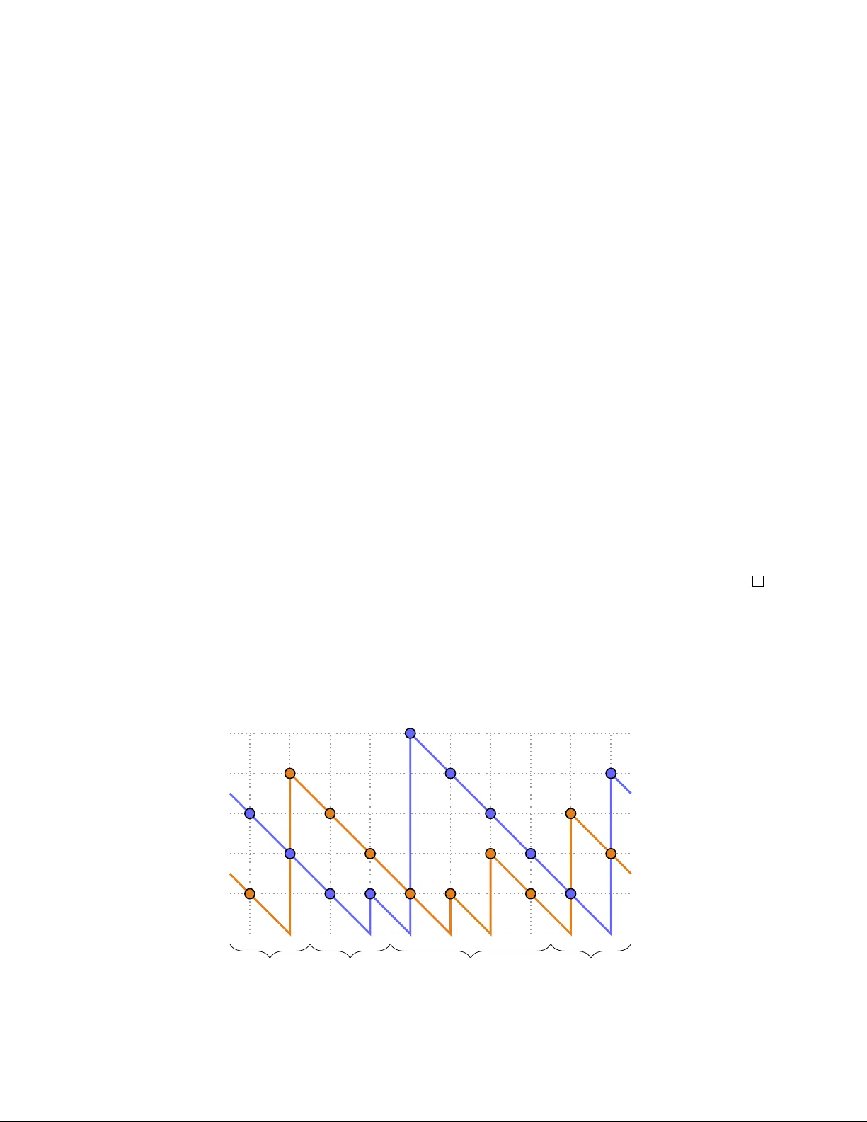
En umerating Prime P atterns in Juggling V ariations Stev e Butler ∗ V era Choi † Jo el Jeffries ‡ Nina McCam bridge § Asia Morgenstern ¶ Sam uel Orellana Mateo ‖ Abstract Juggling patterns can b e mathematically modeled as closed walks within directed state graphs. In this paper, we presen t a unified framew ork of unbounded juggling pat- terns and its v ariations (including m ultiplex, colored, and passing) primarily through the formalism of the juggling state. By extending this state-based approach and uti- lizing com binatorial tools suc h as set partitions and filled F errers diagrams, w e find and prov e a new lo wer b ound on the num b er of b -ball prime patterns with p erio d n . F urther, w e determine exact counts for 2-ball m ultiplex, 1-ball passing, and 2-ball col- ored juggling patterns, as well as a low er b ound for 2-ball passing. W e also pro vide an extensive analysis of the asymptotic growth rates for these pattern counts. Finally , w e formalize the infinite state graph, G ∞ , and utilize flip-reverse in v olutions to estab- lish bijections b et ween classes of prime patterns, exploring how fixing a sp ecific state influences the en umeration of prime walks. ∗ Io w a State Univ ersity , Ames, IA 50011, USA. butler@iastate.edu † T ufts Universit y , Medford, MA 02155, USA. vera.choi@tufts.edu ‡ Io w a State Univ ersity , Ames, IA 50011, USA. joel.a.jeffries@gmail.com § Carnegie Mellon Univ ersit y , Pittsburgh, P A 15213, USA. nmccambr@andrew.cmu.edu ¶ W estminster College, New Wilmington, P A 16172, USA. Current address: Univ ersit y of Kentuc ky , Lexington, KY 40506, USA. asia.morgenstern@gmail.com ‖ Duk e Univ ersit y , Durham, NC 27708, USA. samuelorellanamateo@gmail.com 1 1 In tro duction 1.1 State Graph Juggling, an art form celebrated for its physical dexterity , also has a ric h mathematical structure. The connections b etw een juggling and combinatorics are particularly strong, with the state graph as a formalism dev elop ed to describ e and analyze juggling patterns. In this mo del, a juggling state is represented by a binary v ector indicating the future landing times of the balls. F or instance, in a b -ball pattern, a state is a v ector with exactly b ones. A 1 in p osition i signifies that a ball is scheduled to land i time b eats from the presen t. A directed edge connects tw o states if one can legally transition to the other in a s ingle b eat. If the first entry is a 0, then no ball will land in the next time b eat, hence achieving the only p ossible transition b y deleting that en try . If the first en try is a 1, then a ball lands; w e delete the first entry and we replace any 0 by a 1, representing a throw of the ball that just landed. While Buhler et al. [ Buh+94 ] formally mo del juggling patterns as p ermutations of in te- gers f : Z → Z where f ( t ) ≥ t , w e rely entirely on the state graph formalism. F ormally , given a num b er of balls b , if α = ⟨ α 1 , α 2 , . . . ⟩ and β = ⟨ β 1 , β 2 , . . . ⟩ are tw o states where α i , β j ∈ { 0 , 1 } for all i, j , then α → β is a p ossible transition if and only if α i +1 ≤ β i for all i = 1 , 2 , . . . and ∞ X i =1 α i = ∞ X i =1 β i = b A p erio dic juggling pattern of length n corresp onds to a closed walk of length n in this infinite state graph. This is a subgraph for b = 2 drawn by [ Ban+16 ]: ⟨ 0 , 1 , 0 , 1 ⟩ ⟨ 1 , 0 , 1 , 0 ⟩ ⟨ 1 , 1 , 0 , 0 ⟩ ⟨ 0 , 0 , 1 , 1 ⟩ ⟨ 1 , 0 , 0 , 1 ⟩ ⟨ 0 , 1 , 1 , 0 ⟩ 0 4 1 3 2 2 4 0 4 0 1 3 Figure 1: A subgraph of the tw o-ball state graph. The edge lab els corresp ond to throw heigh ts. While the total num b er of juggling patterns of a giv en length is w ell-understo o d, a more c hallenging problem is to en umerate the prime juggling patterns . A pattern is defined as prime if its corresp onding closed walk in the state graph is a cycle, meaning it visits n distinct states b efore returning to the start. These prime patterns are fundamen tal, as an y juggling pattern can be decomp osed into a sequence of them. This concept is iden tical to what Polster [ P ol03 ] refers to as “prime lo ops” or what Banian et al. [ Ban+16 ] define as “prime cycles”. While P olster mainly bounds state graphs by a maximum throw height h , 2 our definitions allow for un b ounded heights. F urthermore, this differentiates them from the “primitiv e” sequences enumerated by Butler and Graham [ BG10 ], whic h only require the starting state to not b e revisited. 1.2 W ork on prime patterns and formalization Significan t progress on this problem w as made in the pap er Counting prime juggling p atterns b y Banaian, Butler, et al. [ Ban+16 ], which is a foundational reference for our w ork. F or the case of tw o balls ( b = 2), they established a bijection b etw een prime patterns of length n and ordered collections of sets of “spacings” (the distance b et ween the t w o balls in the air). The largest elements of these sets form a partition of n in to distinct parts. This connection allo wed them to derive a formula for P ′ (2 , n ), the num b er of t wo-ball prime patterns of length n . This pap er lo oks at prime patterns by defining a bijection b etw een them and series of sets with certain conditions, one b eing that it is cyclic (suc h that S 1 , S 2 , S 3 represen ts the same pattern as S 2 , S 3 , S 1 ). The prop osition they use, whic h they don’t explicitly state, but lies on their argument for the main result, is the follo wing: Lemma 1.1. L et X t,n the set of al l X t,n = ( S 1 , . . . , S t ) (up to cyclic or der), wher e n = t X i =1 max( S i ) and S i ∩ S j = ∅ for al l 1 ≤ i < j ≤ t . This is p ossibly empty if t is not lar ge enough. Then, ther e is a bije ction b etwe en the set of prime p atterns ρ of length n that c ontain t C 2 c ar ds in their c onstruction, and elements in X t,n . A key result from [ Ban+16 ] that w e will use extensively is the function c t ( n ), which coun ts the num b er of wa ys to form v alid, prime-generating spacing sets where the largest spacings come from a partition of n into t distinct parts. Essen tially: Definition 1.1. c t ( n ) = |X t,n | Then, by using F errers diagram and a coun ting argument, [ Ban+16 ] shows that: Prop osition 1.2. c t ( n ) = X p 1 > ··· >p t ≥ 1 p 1 + ··· + p t = n 1 t ( t + 1) t Y i =1  i + 1 i  p i An immediate consequence of this is that the total num b er of normal prime patterns is N ′ (2 , n ) = P t c t ( n ). Asymptotically , they sho w ed that N ′ (2 , n ) ∼ γ · 2 n for a constant γ ≈ 1 . 3296. While Banaian et al. utilized the c t ( n ) function strictly for normal 2-ball patterns, we demonstrate the versatilit y of this function in later sections by using it as a building blo ck for other coun ts. 3 1.3 V ariations of Juggling The w ork of Buhler, Eisen bud, Graham, and W right, “Juggling Drops and Descen ts” [ Buh+94 ], laid the mathematical foundation for the mo dern analysis of juggling patterns. They es- tablished many of the core concepts, formalizing juggling patterns as p ermutations of the in tegers [ Buh+94 ] and providing the condition for a sequence of thro ws to constitute a v alid pattern [ Buh+94 ]. A k ey con tribution of their work was the in tro duction of the function N ( b, n ), whic h counts the num b er of p erio dic juggling patterns with n b eats and b balls [ Buh+94 ]. This function serves as the primary inspiration for our researc h, as w e seek to define and analyze analogous coun ting functions for different juggling v ariations and for the more restrictive class of prime patterns. The pap er by Bass and Butler [ BB24 ] explores the enumeration of juggling passing pat- terns within a “saturated” model, where all k jugglers are assumed to be activ e on ev ery beat of the pattern. By counting this sp ecific set of patterns in tw o distinct wa ys, the authors pro vide a combinatorial pro of of a generalized W orpitzky’s identit y . They use generalized Eulerian num b ers and ro ok placemen ts on a ( k n ) × n b oard, and while this counts all v alid sequences, it do es not fo cus on prime patterns. W e, in contrast, analyze a differen t “sparse” system by fo cusing on prime patterns with a fixed, small num b er of balls (one or tw o), a scenario where not all hands are necessarily activ e, finding an exact coun t for P ′ (1 , n, k ) and a low er b ound for P ′ (2 , n, k ). In a note added in pro of to their 1994 pap er, Buhler et al. [ Buh+94 ] men tioned that the foundational work b y Ehrenborg and Readdy [ ER96 ] pioneered the enumeration of multi- plex juggling patterns. They defined patterns as triples ( d, x, a ) and utilized decks of cards indexed by multisets of crossings to derive their main q -analogue identities. Ho wev er, when coun ting physically distinct prime patterns this abstraction, their reliance on “in ternal cross- ings” implies that a bijection b etw een card sequences and unique juggling states cannot b e established. P olster [ Pol03 ] also explored m ultiplex state graphs, relying on a brack et nota- tion (for example, [11]10) to group balls landing simultaneously . Hence, w e redefine these concepts. A more rigorous framework for m ultiplex juggling was later pro vided by Butler and Gra- ham [ BG10 ], who transformed the problem of counting sequences in to one of filling a binary matrix sub ject to sp ecific constraints. While their w ork successfully enumerated p erio dic and primitiv e sequences, they explicitly posed the en umeration of prime m ultiplex sequences as an open problem. Building on this foundation, we narrow our focus to the exact en umeration of these prime patterns, sp ecifically for t w o balls. By transitioning from P olster’s brac ket no- tation to a concrete coordinate notation σ ( i,j ) , and defining a new, unam biguous set of cards ( D 0 , D a , D b , D c ), we ha ve a one-to-one corresp ondence b et ween our card sequences and the prime patterns themselv es. This isolates the internal crossings describ ed by Ehrenborg and Readdy (captured b y our D b card) and giv es an exact count for M ′ (2 , n ), thereb y resolving Butler and Graham’s op en problem for the tw o-ball case. 1.4 Infinite State Graph T o study the broader implications of juggling, researc hers hav e also explored infinite state mo dels. Banaian et al. [ Ban+16 ] observ ed that the state graph for b balls is isomorphic to 4 an induced subgraph of the state graph for b + 1 balls. F urthermore, Kn utson, Lam, and Sp ey er [ KLS13 ] established a connection b et ween juggling patterns and algebraic geometry b y formalizing “virtual juggling states” and “juggling functions.” In their framew ork, the negativ e integers act as a “Dirac sea” of a v ailable balls, and patterns are mo deled as affine p erm utations f : Z → Z in the extended affine W eyl group ˜ A n − 1 , where f ( t ) denotes the landing time of a ball thro wn at time t . This infinite mo deling allows for the analysis of prop erties indep enden t of a finite n um- b er of balls. This has b een relev an t in mo dern combinatorics; for instance, Galashin and Lam [ GL24 ] used b ounded affine p erm utations and juggling crossing statistics to compute p ositroid Catalan num b ers, linking juggling math to knot inv arian ts and Kho v ano v-Rozansky homology . In Section 7 , w e build up on this legacy by formally defining the infinite state graph G ∞ . Notice that our abbreviated infinite binary sequences conceptually mirror the “virtual juggling states” of Kn utson et al., allo wing us to establish bijections b et ween walk lengths b y utilizing flip-reverse in volutions across the infinite graph. Our formalization of G ∞ pro vides a direct answ er to an op en question posed at the conclusion of Buhler et al.’s app endix [ Buh+94 ]: “How c an these ide as b e use d to describ e, or ’name,’ juggling p atterns with infinitely many b al ls?” . 1.5 Cards Notation Another w a y to represen t juggling patterns is using their cards. A b -ball juggling pattern can b e represented using b + 1 cards, C 0 , C 1 , . . . , C b , where C 0 means no ball landed, and C i means a ball landed and it w as thro wn to b e now in relative p osition i . These cards are w ell studied, and a v alid pattern represented by states has a known bijection with its card represen tation (see [ Buh+94 ; Pol03 ; Ban+16 ]). It is also imp ortan t to note that our use of cards differs from the definition used by Bass and Butler [ BB24 ]. Ev ery b eat in a juggling pattern has a corresp onding card. C 0 C 1 C 2 Figure 2: Cards for b = 2 F or example, in Fig. 1 , the pattern ⟨ 0 , 1 , 1 , 0 ⟩ → ⟨ 1 , 1 , 0 , 0 ⟩ → ⟨ 1 , 0 , 0 , 1 ⟩ → ⟨ 0 , 1 , 1 , 0 ⟩ of length 3 can also b e represen ted by the sequence C 0 C 2 C 1 or any rotation of these. F or example, in Fig. 1 , the pattern ⟨ 0 , 1 , 1 , 0 ⟩ → ⟨ 1 , 1 , 0 , 0 ⟩ → ⟨ 1 , 0 , 0 , 1 ⟩ → ⟨ 0 , 1 , 1 , 0 ⟩ of length 3 can also b e represented b y the sequence C 0 C 2 C 1 or any rotation of these. F ollowing the card sequences utilized by Banaian et al. to track relativ e ball order, we will introduce the D cards to unambiguously track simultaneous landings and crossings in multiplex prime patterns. 5 1.6 Our w ork W e tak e the idea of using states to define patterns and extend it to its v ariations (m ultiplex, passing) and introduce a new v ariation: colored. In their concluding remarks, Butler and Graham [ BG10 ] sp eculated on the com binatorial complexity of en umerating walks where balls are distinct rather than iden tical, which our colored v ariation formalizes. W e aim to coun t the num b er of prime patterns for each of these v ariations. T o do this, w e establish a new notation framework. While Banaian et al. [ Ban+16 ] used P ( n, b ) to denote the coun t of normal prime patterns, we redefine normal prime patterns as N ′ ( b, n ) to align with the standard p erio dic pattern notation N ( b, n ) from Buhler et al. [ Buh+94 ]. This allo ws us to reserve P for P assing patterns, M for Multiplex, and C for Colored. W e use cursiv e to refer to the sets of the patterns and the standard Latin letter to refer to the coun t of the resp ectiv e set. State Represen tation Constrain t on En tries Constrain t on k α = ⟨ α 1 , α 2 , . . . ⟩ α i ∈ { 0 , 1 } N/A α = ⟨ α 1 , α 2 , . . . ⟩ α i ∈ { 0 , 1 , . . . , k } k apacit y p er hand k ≤ b α = ⟨ α 1 , α 2 , . . . ⟩ α i ∈ { 0 , 1 , 1 , . . . , 1 | {z } k } n umber of k olors k ≤ b A = ( α i,j ), a k × ∞ matrix σ i,j ∈ { 0 , 1 } n umber of hands k ∈ Z T able 1: State representations and constrain ts for juggling v ariations. Where P ∞ i =1 α i = b , or P k i =1 P ∞ j =1 α i,j = b for the last case. The condition for a v alid transition α → β is α i +1 ≤ β i for i = 1 , 2 , . . . , and the inv arian t of the sum being b . Similarly , for passing, the condition for a v alid transition A → B is α i,j +1 ≤ β i,j for i = 1 , 2 , . . . , k and j = 1 , 2 , . . . , again resp ecting the inv arian t. Juggling V ariation P erio dic Patterns Prime P atterns Normal N ( b, n ) N ( b, n ) N ′ ( b, n ) N ′ ( b, n ) Multiplex M ( b, n, k ) M ( b, n, k ) M ′ ( b, n, k ) M ′ ( b, n, k ) Colored C ( b, n, k ) C ( b, n, k ) C ′ ( b, n, k ) C ′ ( b, n, k ) P assing P ( b, n, k ) P ( b, n, k ) P ′ ( b, n, k ) P ′ ( b, n, k ) T able 2: Notation for the sets (cursiv e) and coun ts (latin) of juggling patterns. Here, b is the num b er of balls, n is the p erio d, m is the multiplex capacit y , and k is the num b er of colors or hands. This pap er builds up on the framework established ab o ve. A general form ula for N ( b, n ) w as found using Mobius inv ersion by Buhler et al [ Buh+94 ] in 1994. Then, in 2015, an exact coun t for N ′ (2 , n ) was found by Banaian et al [ Ban+16 ]. 6 W e extend this work b y pro viding an exact count for M ′ (2 , n ) = M ′ (2 , n, 2) in Section 3 and also an exact count for C ′ (2 , n ) = C ′ (2 , n, 2) in Section 4 , basing our argument on the c t ( n ) function dev elop ed b y [ Ban+16 ]. W e also find an exact count for P ′ (1 , n, k ) in Section 5.1 and a low er b ound for P ′ (2 , n, k ) in Section 5.3 . Additionally , w e impro ve the curren tly standing low er b ound for N ′ ( b, n ), which was 1 b b n , presented in [ Ban+16 ]. Finally , Section 7 , we introduce a result that examines the structure of the state graph for an infinite n umber of balls and establishes a bijection b et ween classes of prime patterns. 2 Asymptotics for c t ( n ) 2.1 Preliminaries W e start with some definitions that can b e found in [ Ban+16 ]. W e use these to develop a general theory of functions that define the b ehavior of juggling functions. Definition 2.1. F or integers t ≥ 1 and n ≥ 1, the function c t ( n ) is defined as: c t ( n ) = X p 1 > ··· >p t ≥ 1 p 1 + ··· + p t = n 1 t ( t + 1) t Y i =1  i + 1 i  p i The asymptotic b ehavior of c t ( n ) is controlled by t wo sequences, q t and r t . Definition 2.2. The sequence q t is defined by q 1 = 1 / 2 and for t ≥ 2: q t =  t − 1 2 t − t − 1  q t − 1 = 1 2 t Y i =2 i − 1 2 i − i − 1 Definition 2.3. The sequence r t is defined b y the recurrence r 1 = 0, r 2 = 4 √ 3 9 , and for t ≥ 3: r t = t − 1 √ 3 t − t − 1 r t − 1 + 2  2 t t + 1  ( t − 1) / 2 q t − 1 These sequences provide sharp b ounds for c t ( n ). Lemma 2.1. F or al l inte gers t ≥ 1 and n ≥ 1 , the fol lowing ine quality holds: q t 2 n − r t √ 3 n ≤ c t ( n ) ≤ q t 2 n Summing c t ( n ) ov er all p ossible v alues of t gives the function P ′ (2 , n ). Definition 2.4. P ′ (2 , n ) = ∞ X t =1 c t ( n ) The b ounds on c t ( n ) lead to the asymptotic b eha vior of P (2 , n ). Theorem 2.2. L et γ = P ∞ t =1 q t . The function P ′ (2 , n ) has the asymptotic b ehavior: ( γ − o n (1))2 n ≤ P ′ (2 , n ) ≤ γ 2 n 7 2.2 General Asymptotic Theorem Theorem 2.3 (General Asymptotic Theorem) . L et w : Z + → R ≥ 0 b e a se quenc e of non- ne gative weights. Define the c onstant γ w = P ∞ t =1 w ( t ) q t , and assume this series c onver ges. L et F w ( n ) = P ∞ t =1 w ( t ) c t ( n ) . Then, as n → ∞ : 1. F w ( n ) = ( γ w − o (1))2 n . 2. S w ( n ) := P n − 1 m =1 F w ( m ) = ( γ w − o (1))2 n . 3. ( F w ∗ F w )( n ) := P n − 1 m =1 F w ( m ) F w ( n − m ) = ( γ 2 w − o (1)) n 2 n . Pr o of. The pro of relies on the b ounds for c t ( n ) from Theorem 2.1 : q t 2 n − r t √ 3 n ≤ c t ( n ) ≤ q t 2 n . First, we work on the asymptotics of F w ( n ). W e start by establishing the upp er b ound. Since w ( t ) ≥ 0 for all t , w e hav e: F w ( n ) = ∞ X t =1 w ( t ) c t ( n ) ≤ ∞ X t =1 w ( t )( q t 2 n ) = ∞ X t =1 w ( t ) q t ! 2 n = γ w 2 n . This implies lim sup n →∞ F w ( n ) 2 n ≤ γ w . F or the low er b ound, let ε > 0. Since the series for γ w con verges, we can choose an in teger K large enough such that P K t =1 w ( t ) q t > γ w − ε 2 . Let γ w,K = P K t =1 w ( t ) q t and ρ w,K = P K t =1 w ( t ) r t . Note that ρ w,K is a finite sum and th us well-defined. Since w ( t ) ≥ 0 and c t ( n ) ≥ 0, w e can truncate the sum for a low er b ound: F w ( n ) = ∞ X t =1 w ( t ) c t ( n ) ≥ K X t =1 w ( t ) c t ( n ) ≥ K X t =1 w ( t )( q t 2 n − r t √ 3 n ) = K X t =1 w ( t ) q t ! 2 n − K X t =1 w ( t ) r t ! √ 3 n = γ w,K 2 n − ρ w,K √ 3 n . Using our c hoice of K , w e hav e F w ( n ) > ( γ w − ε 2 )2 n − ρ w,K √ 3 n . W e w ant to show that for sufficien tly large n , this is greater than ( γ w − ε )2 n . This is equiv alent to sho wing ε 2 2 n > ρ w,K √ 3 n , which simplifies to ε 2 ρ w,K > ( √ 3 2 ) n . Since √ 3 2 < 1, the righ t-hand side approac hes 0 as n → ∞ . Th us, for an y fixed ε and K , there exists an N such that the inequalit y holds for all n > N . This sho ws that for an y ε > 0, F w ( n ) > ( γ w − ε )2 n for sufficiently large n . This implies lim inf n →∞ F w ( n ) 2 n ≥ γ w . Com bining the limsup and liminf results, we conclude that lim n →∞ F w ( n ) 2 n = γ w . 8 Second, we work on the asymptotics of S w ( n ). F or the upp er b ound, we sum the upp er b ound for F w ( m ): S w ( n ) = n − 1 X m =1 F w ( m ) ≤ n − 1 X m =1 γ w 2 m = γ w (2 n − 2) ≤ γ w 2 n . This implies lim sup n →∞ S w ( n ) 2 n ≤ γ w . F or the low er b ound, we use the same truncation argument. F or a giv en ε > 0, choose K such that γ w,K = P K t =1 w ( t ) q t > γ w − ε 2 . S w ( n ) = n − 1 X m =1 F w ( m ) ≥ n − 1 X m =1 K X t =1 w ( t ) c t ( m ) ! ≥ n − 1 X m =1  γ w,K 2 m − ρ w,K √ 3 m  = γ w,K n − 1 X m =1 2 m − ρ w,K n − 1 X m =1 √ 3 m = γ w,K (2 n − 2) − ρ w,K √ 3(( √ 3) n − 1 − 1) √ 3 − 1 . Dividing by 2 n , we get S w ( n ) 2 n ≥ γ w,K (1 − 2 / 2 n ) − ρ w,K √ 3 − 1 √ 3 2 ! n − √ 3 2 n ! . T aking the limit inferior as n → ∞ : lim inf n →∞ S w ( n ) 2 n ≥ γ w,K (1 − 0) − ρ w,K √ 3 − 1 (0 − 0) = γ w,K . Since w e can c ho ose K suc h that γ w,K is arbitrarily close to γ w , it follows that lim inf n →∞ S w ( n ) 2 n ≥ γ w . Com bining the limsup and liminf results, we conclude that lim n →∞ S w ( n ) 2 n = γ w . Finally , w e study the asymptotics of ( F w ∗ F w )( n ). The upp er b ound is found b y substi- tuting the upp er b ound for F w : ( F w ∗ F w )( n ) = n − 1 X m =1 F w ( m ) F w ( n − m ) ≤ n − 1 X m =1 ( γ w 2 m )( γ w 2 n − m ) = n − 1 X m =1 γ 2 w 2 n = ( n − 1) γ 2 w 2 n . Dividing by n 2 n giv es ( F w ∗ F w )( n ) n 2 n ≤ n − 1 n γ 2 w . T aking the limit sup erior, we get lim sup n →∞ ( F w ∗ F w )( n ) n 2 n ≤ γ 2 w . F or the lo wer b ound, let ε > 0 and c ho ose K such that γ w,K > γ w − ε . Since F w ( k ) ≥ 0, w e ha v e ( F w ∗ F w )( n ) ≥ ( F w,K ∗ F w,K )( n ), where F w,K ( k ) = P K t =1 w ( t ) c t ( k ). Let F w,K ( k ) = 9 γ w,K 2 k − E K ( k ), where 0 ≤ E K ( k ) ≤ ρ w,K √ 3 k . ( F w,K ∗ F w,K )( n ) = n − 1 X m =1 ( γ w,K 2 m − E K ( m ))( γ w,K 2 n − m − E K ( n − m )) = n − 1 X m =1 γ 2 w,K 2 n − γ w,K n − 1 X m =1 (2 m E K ( n − m ) + 2 n − m E K ( m )) + n − 1 X m =1 E K ( m ) E K ( n − m ) . The main term is ( n − 1) γ 2 w,K 2 n . The error terms are of a smaller order. The second term is bounded by O (2 n ) and the third b y O ( n √ 3 n ). So, ( F w,K ∗ F w,K )( n ) = ( n − 1) γ 2 w,K 2 n − O (2 n ) − O ( n √ 3 n ). Dividing b y n 2 n : ( F w,K ∗ F w,K )( n ) n 2 n = n − 1 n γ 2 w,K − O (1 /n ) − O (( √ 3 / 2) n ) . T aking the limit as n → ∞ , we get lim n →∞ ( F w,K ∗ F w,K )( n ) n 2 n = γ 2 w,K . Therefore, lim inf n →∞ ( F w ∗ F w )( n ) n 2 n ≥ lim n →∞ ( F w,K ∗ F w,K )( n ) n 2 n = γ 2 w,K > ( γ w − ε ) 2 . Since this holds for an y ε > 0, we can let ε → 0 to find that lim inf n →∞ ( F w ∗ F w )( n ) n 2 n ≥ γ 2 w . Com bining the limsup and liminf results, we conclude that lim n →∞ ( F w ∗ F w )( n ) n 2 n = γ 2 w . Corollary 2.4. L et w : Z + → R ≥ 0 b e a se quenc e of non-ne gative weights. Define the c onstant γ w = P ∞ t =1 w ( t ) q t , and assume this series c onver ges. L et F w ( n ) = P ∞ t =1 w ( t ) c t ( n ) . Then, as n → ∞ : 1. F w ( n ) ∼ γ w 2 n . 2. S w ( n ) := P n − 1 m =1 F w ( m ) ∼ γ w 2 n . 3. ( F w ∗ F w )( n ) := P n − 1 m =1 F w ( m ) F w ( n − m ) ∼ γ 2 w n 2 n . 3 Multiplex 2-Ball 3.1 Preliminaries Multiplex juggling is a v ariation of normal juggling that allows for the sim ultaneous toss of m ultiple balls in a single time b eat. Unlik e standard juggling, where each throw and catch in volv es only one ball at a time, multiplex juggling in tro duces the p ossibility of throwing m ultiple balls within the same hand. In other words, w e increase the capacit y of our juggling hands, unlo cking for example the transition ⟨ 1 , 0 , 1 ⟩ → ⟨ 0 , 2 ⟩ . Concretely , w e can set the k apacit y of eac h hand to b e k ≤ b . Hence, a state σ is not restricted anymore to having only 1’s, as no w, a i ∈ { 0 , 1 , 2 , . . . , k } . How ever, we still ha ve the condition that P i a i = b . F or example, if we set b = 3 and k = 2, we can ha ve the state σ = ⟨ 0 , 2 , 1 ⟩ . After one b eat, all balls fall, so σ → σ ′ where σ ′ = ⟨ 2 , 1 ⟩ . Then, w e ha v e infinitely man y choices for σ ′′ 10 suc h that σ ′ → σ ′′ since the tw o balls in the first p osition can go anywhere. Some p ossible states include ⟨ 1 , 0 , 2 ⟩ , ⟨ 1 , 1 , 0 , 1 ⟩ , and ⟨ 2 , 1 ⟩ . F or all of them, a 1 ≥ 0, and the only throw that would not b e allo wed is ⟨ 3 ⟩ , as k = 2 do es not allow 3 balls to b e in the same b eat. Fig. 3 shows some p ossible transitions in M (3 , n, 2). h 1 , 1 , 1 i h 0 , 2 , 1 i h 2 , 1 i h 2 , 0 , 1 i h 1 , 0 , 2 i h 0 , 1 , 2 i h 1 , 2 i Figure 3: A p ortion of the state diagram when b = 3 and k = 2. This section will fo cus in 2-ball multiplex prime patterns. W e aim to expand the metho d used in [ Ban+16 ] in order to find a count for M ′ (2 , n ). As w e are only going to lo ok at b = 2, we will assume that k is alwa ys 2 (as k = 1 is equiv alent to normal juggling). Hence, all states will contain either one 2 and p ossibly 0’s or tw o 1’s and p ossibly 0’s. F or example, this w ould b e a v alid 2-ball m ultiplex juggling pattern: ⟨ 0 , 0 , 2 ⟩ → ⟨ 0 , 2 ⟩ → ⟨ 2 ⟩ → ⟨ 0 , 1 , 0 , 0 , 1 ⟩ → ⟨ 1 , 0 , 0 , 1 ⟩ → ⟨ 0 , 1 , 1 ⟩ → ⟨ 1 , 1 ⟩ → ⟨ 1 , 0 , 0 , 0 , 1 ⟩ → ⟨ 0 , 0 , 0 , 2 ⟩ → ⟨ 0 , 0 , 2 ⟩ F or the graphical represen tation, we will add double lines and double circles to represent states and transitions with tw o balls. As an example, Fig. 4 shows the pattern describ ed ab o ve, but graphically . Figure 4: An example of a 2-ball m ultiplex pattern. F urthermore, w e will in tro duce a new notation for m ultiplex 2-ball states that will simplify future pro cesses: σ ( i,j ) = ⟨ 0 , . . . , 0 , 1 | {z } i , 0 , . . . , 0 , 1 | {z } j ⟩ 11 where 1 ≤ i ≤ j . Essen tially , eac h “co ordinate” denotes the p osition of one ball. The definition sho ws the case when i < j but in m ultiplex juggling, w e can define that i = j when b oth the first and second balls are indistinguishably in the same p osition: σ ( i,i ) = ⟨ 0 , . . . , 0 , 2 | {z } i | {z } i ⟩ W e prop ose a generalization of this notation that could b e useful for future analysis of m ultiplex b -ball prime patterns: σ ( i,j,k,... ) = ⟨ 0 , . . . , 0 , 1 | {z } i , 0 , . . . , 0 , 1 | {z } j , 0 , . . . , 0 , 1 | {z } k , . . . | {z } ... ⟩ 3.2 Set Notation In this section, we will follo w a similar pro cess to the one used to solv e the n umber of normal 2-ball juggling patterns. In order to simplify , we will often omit the fact that all patterns in this section are 2-ball patterns. A first realization is that N ′ (2 , n ) ⊆ M ′ (2 , n ), b ecause an y normal pattern can be consid- ered a multiplex pattern and primeness is preserved. This leads to the follo wing definition: Definition 3.1. Let ρ denote a juggling pattern. The set of strict-multiplex patterns , denoted M ′ (2 , n ), is defined as follo ws: M ′ \ N ′ (2 , n ) = { ρ ∈ M ′ (2 , n ) | ρ / ∈ N ′ (2 , n ) } , where M ′ (2 , n ) represen ts the set of all multiplex 2-ball prime patterns, and N ′ (2 , n ) repre- sen ts the set of all normal 2-ball prime patterns. This allo ws us to count only the new patterns added to M ′ (2 , n ) b y increasing hand capacit y . Now, w e introduce a fundamen tal prop erty of these m ultiplex patterns. Lemma 3.1. A 2-b al l strict multiplex prime p attern c ontains the state ⟨ 2 ⟩ exactly onc e. Pr o of. Let ρ b e a strict multiplex prime pattern. By primeness, each state ⟨ 2 ⟩ can app ear at most once within ρ . Now it remains to prov e that it app ears at least once. Supp ose initially that no state in ρ tak es the form σ i,i . Then, ev ery state must b e of the form σ i,j where i < j . This condition implies that ρ ∈ N ′ (2 , n ) and consequen tly ρ / ∈ M ′ \ N ′ (2 , n ), which leads to a con tradiction. Therefore, there exists at least one state σ i,i ∈ ρ for some i . If i = 1, then σ 1 , 1 = ⟨ 2 ⟩ app ears in ρ . If not, the only p ossible transition from σ i,i is σ i,i → σ i − 1 ,i − 1 → · · · → σ 1 , 1 = ⟨ 2 ⟩ . 12 Theorem 3.1 implies that a strict m ultiplex pattern can never b e written using C 0 , C 1 and C 2 cards, b ecause we need cards that represent throws in volving tw o balls. W e introduce four new cards, D 0 , D a , D b and D c that represen t all p ossible throws b et ween states inv olving multiplex with tw o balls. These cards are graphically represen ted in Fig. 5 , where a thic k line represents t wo balls b eing in the same b eat. D 0 D a D b D c Figure 5: New cards used in strict m ultiplex patterns • D 0 represen ts the transition σ ( i,i ) → σ ( i − 1 ,i − 1) . • D a represen ts the transition σ (1 ,i ) → σ ( i − 1 ,i − 1) . • D b represen ts the transition σ (1 , 1) → σ ( i,j ) , with i < j . • D c represen ts the transition σ (1 , 1) → σ ( i,i ) . The D c card is a rare card among prime patterns. Given a fixed length n , there is exactly one ρ ∈ M ′ \ N ′ (2 , n ) such that D c ∈ ρ . That pattern is σ ( n,n ) → σ ( n − 1 ,n − 1) → · · · → σ (1 , 1) → σ ( n,n ) Hence, we can count all patterns such that D c / ∈ ρ . Any prime pattern will hav e a sequence of cards with the form D a , D 0 , D 0 , . . . , D 0 , D b . Supp ose w e place those balls at the end of the pattern. 3.3 Main Theorem Theorem 3.2. L et M ′ \ N ′ ( n, 2) b e the numb er of 2-b al l strict multiplex prime juggling p atterns of p erio d n . Then M ′ ( n, 2) = X t n − 1 X m =1 t · c t ( m ) ! + 1 Pr o of of The or em 3.2 . Let ρ ∈ M ′ \ N ′ ( n, 2). Notice that we can see this juggling pattern that b egins with the state σ (1 , 1) , immediately after it transitions to σ ( i,j ) and even tually reac hes σ (1 ,j − i +1) . Then b eha ves as a normal prime pattern, and we can describ e this b ehavior through sets S 1 , S 2 , . . . , S t . Finally , when the smallest space of the last spacing happ ens, sa y a space k , the transition σ (1 , 1+ k ) → σ ( k,k ) , whic h ev entually reac hes σ (1 , 1) and closes the cycle. Notice how here, if i = 1, we started with a pattern ρ ∈ M ′ \ N ′ ( n, 2) and we obtained sets S 1 , S 2 , . . . , S t that define a pattern ρ ′ ∈ N ′ ( n − 1 , 2) (as we remo v e the multiplex thro w). 13 Ho wev er, for an y i , a pattern ρ ∈ M \ N ′ ( n, 2) giv es sets S 1 , S 2 , . . . , S t that define a pattern ρ ′ ∈ N ′ ( n − i, 2). Reasoning backw ards, for all i > 0 we can take a pattern ρ ′ ∈ N ′ ( n − i, 2), obtain its sets S 1 , S 2 , . . . , S t and place the multiplex throw in t differen t p ositions (b ecause of the cyclic structure), obtaining t different patterns ρ j ∈ M ′ \ N ′ ( n, 2) for j = 1 , 2 , . . . , t . The theorem follo ws directly from the uniqueness of these ρ j giv en an initial ρ ′ , and the +1 comes from the pattern σ ( n,n ) → · · · → σ (1 , 1) . Giv en Theorem 3.2 , the follo wing follows directly Corollary 3.3. L et M ′ ( n, 2) b e the numb er of 2-b al l multiplex prime juggling p atterns of p erio d n . Then M ′ ( n, 2) = X t c t ( n ) + n − 1 X m =1 t · c t ( m ) ! + 1 3.4 Asymptotics W e present the exact v alues of M ′ ( n, 2) for small n in T able 3 . n M ′ ( n, 2) 1 2 2 4 3 9 4 20 5 45 6 100 7 223 8 484 9 1053 10 2258 n M ′ ( n, 2) 11 4827 12 10198 13 21505 14 44920 15 93687 16 194072 17 401061 18 824710 19 1693027 20 3460930 n M ′ ( n, 2) 21 7064961 22 14377628 23 29219511 24 59240884 25 119980813 26 242531914 27 489839523 28 987879134 29 1990834305 30 4007533072 T able 3: M ′ ( n, 2) for 1 ≤ n ≤ 30 W e now determine the asymptotic b eha vior of M ′ ( n, 2) by applying the General Asymp- totic Theorem ( Theorem 2.3 ) and its corollary ( Theorem 2.4 ). Recall from Theorem 3.2 that the n umber of strict m ultiplex patterns is giv en by M ′ \ N ′ ( n, 2) = n − 1 X m =1 ∞ X t =1 t · c t ( m ) ! + 1 W e define the w eight function w ( t ) = t . The asso ciated constan t is γ M ′ \ N ′ = ∞ X t =1 t · q t Using the definition of q t , this series conv erges. W e identify the inner sum of the expression for M ′ \ N ′ ( n, 2) as F w ( m ) and the outer sum as S w ( n ) from Theorem 2.4 . 14 Lemma 3.4. The numb er of strict multiplex prime p atterns satisfies M ′ \ N ′ ( n, 2) ∼ γ M ′ \ N ′ 2 n as n → ∞ . Pr o of. Let w ( t ) = t . By definition, F w ( m ) = P ∞ t =1 tc t ( m ). The expression for strict multi- plex patterns is M ′ \ N ′ ( n, 2) = n − 1 X m =1 F w ( m ) + 1 = S w ( n ) + 1 By Theorem 2.4 , part 2, w e ha ve S w ( n ) ∼ γ M ′ \ N ′ 2 n . Since the constant term 1 is negligible compared to 2 n , the result follows. W e now consider the total count of m ultiplex prime patterns, M ′ ( n, 2). Theorem 3.5. The numb er of multiplex 2-b al l prime juggling p atterns satisfies M ′ ( n, 2) ∼ γ M ′ 2 n wher e γ M ′ = ∞ X t =1 ( t + 1) q t Pr o of. By definition, M ′ ( n, 2) = M ′ \ N ′ ( n, 2) + N ′ ( n, 2). F or the term N ′ ( n, 2) = P ∞ t =1 c t ( n ), w e apply Theorem 2.4 , part 1, with the w eigh t function v ( t ) = 1. This yields N ′ ( n, 2) ∼ ∞ X t =1 1 · q t ! 2 n = γ N ′ 2 n Com bining this with Theorem 3.4 , we obtain M ′ ( n, 2) ∼ γ M ′ \ N ′ 2 n + γ N ′ 2 n = ( γ M ′ \ N ′ + γ N ′ )2 n The constant is given b y γ M ′ = ∞ X t =1 tq t + ∞ X t =1 q t = ∞ X t =1 ( t + 1) q t This completes the pro of. W e can compute the n umerical v alue of the constant γ M ′ using the formula for q t : γ M ′ = 1 2 (1 + 1) + ∞ X t =2 ( t + 1) 1 2 t Y i =2 i − 1 2 i − i − 1 Using the identit y t ! = t Q t i =2 ( i − 1), w e can rewrite the terms to facilitate computation. 15 4 Colored 2-Ball 4.1 Preliminaries Colored juggling is a v ariation of normal juggling where eac h ball is assigned a color. Unlik e standard juggling, where the balls are t ypically indistinguishable from one another, colored juggling requires to not only k eep track of the n um b er of balls but also their sp ecific colors. F or example, in ⟨ 0 , 0 , 1 , 0 , 0 , 1 ⟩ → ⟨ 0 , 1 , 0 , 0 , 1 ⟩ ⟨ 0 , 0 , 1 , 0 , 0 , 1 ⟩ → ⟨ 0 , 1 , 0 , 0 , 1 ⟩ the first transition is v alid b ecause each balls comes do wn one p osition after a b eat. The second one, how ever, is not v alid b ecause the balls that come down don’t match the original balls. F or colored 2-ball, the first observ ation w e mak e is that for something b eing a pattern, it’s not sufficient that the states match at the end with the b eginning, as w e also need that the colors of the balls matc h. Lemma 4.1. A 2-b al l c olor e d juggling p attern c ontains an even numb er of C 2 c ar ds. Pr o of. By describing a pattern using card notation, we are describing the relative p osition of the balls in eac h time b eat. Note that the cards C 0 and C 1 do not change the relativ e p osition of the balls, and the C 2 alw ays do it. Hence, in order to k eep the relativ e order of the colored balls from the end to cycling to the b eginning, an even num b er of C 2 cards are needed. Hence, a colored 2-ball pattern can b e defined by a collection of 2 n sets S 1 , S 2 , . . . , S 2 t up to rotational symmetry ( S 1 S 2 S 3 is the same as S 2 S 3 S 1 ). The condition for primeness is that a state can b e rep eated only if the corresponding colors are different. F or example ⟨ 0 , 1 , 0 , 0 , 1 ⟩  = ⟨ 0 , 1 , 0 , 0 , 1 ⟩ . T ranslating this in to sets, for a prime pattern w e know a ∈ S i , S j = ⇒ i ≡ j ( mo d 2). Here, as pro ven in [ Ban+16 ] n = P 2 t i max( S i ). S 1 R 1 S 2 R 2 Figure 6: An example of a colored pattern. 16 Another wa y to see this is renaming the initial sets: we can define tw o collections S = S 1 , S 2 , . . . , S t and R = R 1 , R 2 , . . . , R t , which w e assign to b e the ev en and o dd sets up to rotational symmetry . Here, the length of the pattern is n = t X i =1 max( S i ) + max( R i ) The condition for primeness for a colored prime pattern b ecomes ∀ i, j S i ∩ S j = ∅ and R i ∩ R j = ∅ The ab ov e condition implies that, in a 2-ball prime colored pattern, b oth S and R ha ve to represen t normal prime juggling patterns with lengths m and n − m , suc h that b oth ha ve the same num b er of C 2 cards (which is equiv alent as having the same num b er of partitions in the set notation), where n is the length of the colored 2-ball prime juggling pattern. Using this, w e hav e conv erted out task of coun ting juggling patterns into a problem of coun ting collections of sets with certain conditions. W e use sligh tly different metho ds for the cases when n is ev en or n is o dd. 4.2 Main Theorems Theorem 4.2. The numb er of c olor e d 2-b al l prime juggling p atterns of o dd length is C ′ (2 , n ) = n − 1 2 X m =1 X t t · c t ( m ) · c t ( n − m ) Pr o of. W e can assign each colored 2-ball prime juggling pattern to t wo collections S and R as defined ab o ve. Hence, we can count the num b er of w a ys to arrange those collections in order (up to cyclic p erm utation) to count the n umber of desired patterns. First, w e assume without loss of generality that the length of the pattern defined b y S is m and the length of the pattern defined b y R is n − m where m < n − m (th us m < n 2 − 1). Giv en m , if w e let |S | = |R| = t , w e see there are c t ( m ) w ays to arrange v alid collections S and c t ( n − m ) w ays to arrange v alid collections R . As S and R describ e differen t patterns, we kno w that there is at least one pair i, j such that S i  = R j . F urthermore, no t wo elements in S and R are equal. Hence, all t rotations π of R make the arrangemen t S 1 , R π (1) , S 2 , R π (2) , . . . , S t , R π ( t ) differen t under rotational symmetry for eac h π , b ecause the elements S i and R j will ha v e differen t relativ e p ositions on it. Other w ay to see it is that we can place R 1 after S 1 , or after S 2 , etc, and each one will yield a different pattern. Prop osition 4.3. The numb er of c olor e d 2-b al l prime juggling p atterns of even length is C ′ (2 , n ) =   X t n 2 − 1 X m =1 · c t ( m ) · t · c t ( n − m )   + X t t  c t ( n 2 ) 2  +  t 2  c t  n 2  ! 17 Pr o of. The argument of the previous theorem is still v alid for ev ery m < n 2 , which leads to the first term of the form ula. F or the case m = n 2 , for each partition of size t , there are  c t ( n 2 ) 2  w ays to create combi- nations of ( S , R ) with S  = R . F or each pair, there are t w ays to arrange eac h combination in to a colored 2-ball prime juggling pattern. This gives X t t ·  c t  n 2  2  F urthermore, there are c t  n 2  w ays to create combinations of ( S , R ) with S = R , and in this case there are ⌈ t 2 ⌉ w ays to arrange each com bination into a colored 2-ball prime juggling pattern. The reason for is, for t ev en, t 2 out of the t arrangements are equiv alent to each other. F or t o dd, this happ ens t − 1 2 of the times, lea ving t +1 2 v alid placemen ts, as sho wn in Section 4.2 . This gives the term X t l n 2 m · c t  n 2  S 1 S 2 S 3 S 4 S 5 S 1 S 2 S 3 S 4 S 5 S 6 4.3 Asymptotics W e now determine the asymptotic b eha vior of C ′ (2 , n ). W e first establish b ounds for the case when n is even to sho w that the parity of n does not affect the leading asymptotic term. Lemma 4.4. F or any n even 1 2 n − 1 X m =1 X t t · c t ( m ) · c t ( n − m ) ≤ C (2 , n ) ≤ n 2 X m =1 X t t · c t ( m ) · c t ( n − m ) holds. Pr o of. F or n o dd, the sum ranges from 1 to ( n − 1) / 2, meaning there is no middle term m = n/ 2. The inequalit y b ecomes an equalit y , so the statement holds trivially . F or n ev en, the summation terms for m  = n/ 2 are iden tical in all three expressions. Th us, it suffices to v erify the inequality for the sp ecific term where m = n/ 2. W e must sho w: 1 2 t  c t  n 2  2 ≤ t  c t  n 2  2  +  t 2  c t  n 2  ≤ t  c t  n 2  2 18 Expanding the binomial co efficien t in the middle term: t  c t  n 2  2  +  t 2  c t  n 2  = t c t  n 2   c t  n 2  − 1  2 +  t 2  c t  n 2  = 1 2 t  c t  n 2  2 − 1 2 tc t  n 2  +  t 2  c t  n 2  = 1 2 t  c t  n 2  2 + c t  n 2   t 2  − t 2  F or the low er b ound, since c t ( n/ 2) ≥ 0 and ⌈ t/ 2 ⌉ ≥ t/ 2, the term c t ( n/ 2)( ⌈ t/ 2 ⌉ − t/ 2) is non-negativ e. Thus: 1 2 t  c t  n 2  2 ≤ 1 2 t  c t  n 2  2 + c t  n 2   t 2  − t 2  F or the upp er b ound, w e can assume c t ( n/ 2) ≥ 1 and t ≥ 1 (b ecause the inequality is trivially true when c t ( n/ 2) = 0). W e subtract the expanded middle term from the upp er b ound target t ( c t ( n/ 2)) 2 : t  c t  n 2  2 −  1 2 t  c t  n 2  2 + c t  n 2   t 2  − t 2  = 1 2 t  c t  n 2  2 − c t  n 2   t 2  − t 2  = c t  n 2   t 2 c t  n 2  −  t 2  − t 2  and we aim to sho w this is non-negative. W e know that ⌈ t/ 2 ⌉ − t/ 2 is either 0 (if t is ev en) or 1 2 (if t is o dd). Since t ≥ 1 and c t ( n/ 2) ≥ 1, w e ha ve t 2 c t ( n/ 2) ≥ 1 2 . Therefore, t 2 c t ( n/ 2) ≥ ⌈ t/ 2 ⌉ − t/ 2, making the difference non-negativ e. Thus: t  c t  n 2  2  +  t 2  c t  n 2  ≤ t  c t  n 2  2 Summing ov er all t completes the pro of. F urthermore, the difference b et w een the o dd and even formulas asymptotically relative to n 2 n . Consequen tly , the asymptotic b ehavior of the function is indep endent of parit y . W e now apply the General Asymptotic Theorem to find the explicit growth rate. Theorem 4.5. The numb er of c olor e d 2-b al l prime juggling p atterns of length n satisfies C ′ (2 , n ) ∼ γ C ′ n 2 n wher e γ C ′ = 1 2 ∞ X t =1 tq 2 t = 1 8 ∞ X t =1 t t Y i =2 i − 1 2 i − i − 1 ! 2 ≈ 0 . 478326 . 19 Pr o of. Let S ( n ) = P ∞ t =1 t ( c t ∗ c t )( n ). W e apply Theorem 2.3 (Part 3) to the single function c t ( n ) (equiv alent to setting the w eight w ( k ) = δ kt ). The theorem states that the con volution of c t with itself b ehav es as: ( c t ∗ c t )( n ) ∼ q 2 t n 2 n . The term corresp onding to the midp oint m = n/ 2 in the con v olution is c t ( n/ 2) 2 , whic h b y Theorem 2.1 is b ounded b y O (2 n ). This is negligible compared to the total conv olution sum whic h gro ws as O ( n 2 n ). Consequently , the difference b et ween the upp er and lo wer b ounds in Theorem 4.4 v anishes asymptotically relative to the main term, and C ′ (2 , n ) ∼ 1 2 S ( n ) for b oth even and o dd n . Summing the asymptotic contributions o ver t : S ( n ) = ∞ X t =1 t ( c t ∗ c t )( n ) ∼ ∞ X t =1 t ( q 2 t n 2 n ) = ∞ X t =1 tq 2 t ! n 2 n . The exc hange of the summation and the limit is justified b y the uniform b ounds on c t ( n ) pro vided in Theorem 2.1 , whic h ensure the series con verges. Thus, C ′ (2 , n ) ∼ 1 2 ∞ X t =1 tq 2 t ! n 2 n = γ C ′ n 2 n . 5 P assing 1-Ball and 2-Ball A passing pattern is a juggling pattern in whic h balls can b e thro wn and caught with k distinct hands, so that at most k balls can b e caught and thro wn at one time, and they can b e thrown to an y hand. In general, a state in passing is a k × ∞ matrix A , where the sum of all en tries is b , the n umber of balls. If an en try a i,j = 1, it means that a ball is sc heduled to land in j b eats at “hand” n umber i . Similarly to normal juggling, ones mov e to the left once each b eat, and can b e thrown anywhere when they reac h the leftmost column (meaning that a ball has landed at a hand). This is an example of a v alid transition for b = 2, k = 3:  0 0 1 0 1 0  →  0 1 0 1 0 0  P atterns are prime if they nev er rep eat a state. In regular juggling, if a set of spacings b et ween the balls o ccurs more than once, the pattern will not b e prime as they will b oth ev entually reach the state ⟨ 1 , . . . ⟩ . F or example, in 2-ball juggling, having a spacing of j b et ween the balls will ev entually reac h the state ⟨ 1 , 0 , . . . , 1 | {z } j ⟩ in both cases. Ho wev er, in passing, this difference can o ccur if 20 balls are scheduled to land at different hands. F or example: * 0 1 0 0 0 0 0 1 0 0 0 0 +  = * 0 0 0 0 0 1 0 0 0 0 0 1 + but b oth states ha v e a ball landing in 2 b eat and another ball landing in 4 b eats. In general, w e denote by P ( b, n, k ) the n umber of b -ball passing patterns with k hands and length n , and w e use P ( b, n, k ) to denote the n um b er of such prime patterns. F urthermore, w e use P and P ′ to refer to the set of all such patterns, not the count of them: this is, w e can talk ab out a pattern ρ ∈ P . 5.1 P assing 1-Ball In this section we find an exact count for P ′ (1 , n, k ). Theorem 5.1. The numb er of 1-b al l prime p assing p atterns of length n and k hands is P ′ (1 , n, k ) = k X h =1  k h  n − 1 h − 1  ( h − 1)! Pr o of. F or passing patterns with a single ball, k p ossible hands, and n states, we can c ho ose h of the k hands to throw to within the pattern. Notice that w e ma y not thro w to any giv en hand more than once in a one-ball pattern, b ecause that would rep eat the state of the ball landing in that hand. Therefore, for each of  k h  c hoices, for each hand in h , the ball may b e thrown to one heigh t ab ov e that hand. As the heigh ts of the throws must sum to the cycle length n when w e hav e only one ball, w e get the heigh ts by a partition of n into h parts. There are therefore (b y applying Stars and Bars)  k h  n − 1 h − 1  p ossible heights for an y 1 ≤ h ≤ k . Giv en that the pattern dep ends on the order of the heigh ts up to rotation, of which there are ( h − 1)! p ossibilities. Summing ov er all p ossible num b ers of activ e hands h from 1 to k giv es the total coun t. 5.2 Asymptotic Beha vior of P ′ (1 , n, k ) In this section, w e analyze the behavior of the function P ′ (1 , n, k ). the form ula deriv ed in Section 5.1 is a p olynomial in k , and for a fixed k , it is a p olynomial in n . 5.2.1 Case 1: Fixed n , k → ∞ When n is fixed, the n umber of hands k can grow indefinitely . The sum is limited b y h ≤ n , so: P ′ (1 , n, k ) = n X h =1  k h  n − 1 h − 1  ( h − 1)! 21 Prop osition 5.2. F or a fixe d inte ger n ≥ 1 , as k → ∞ , the numb er of prime 1-b al l, k -hand p assing p atterns of length n b ehaves as: P ′ (1 , n, k ) ∼ k n n Pr o of. Each term in the finite sum is a p olynomial in k . The term  k h  = k ( k − 1) ··· ( k − h +1) h ! is a p olynomial in k of degree h . Therefore, the en tire sum P ′ (1 , n, k ) is a p olynomial in k . The degree of this p olynomial is determined b y the largest v alue of h in the sum, whic h is h = n . W e can analyze the term for h = n : T erm h = n =  k n  n − 1 n − 1  ( n − 1)! =  k n  · 1 · ( n − 1)! = k ( k − 1) · · · ( k − n + 1) n ! ( n − 1)! = k ( k − 1) · · · ( k − n + 1) n This is a p olynomial in k of degree n . The leading term is k n n . No w consider an y other term for h < n . The degree of this term as a p olynomial in k is h . Since all other terms hav e a degree strictly less than n , the asymptotic b eha vior of P ′ (1 , n, k ) for large k is dominated by the h = n term. No w we can write the sum as: P ′ (1 , n, k ) = k ( k − 1) · · · ( k − n + 1) n + n − 1 X h =1  k h  n − 1 h − 1  ( h − 1)! The first term is a p olynomial in k of degree n with leading term k n n . The summation is a p olynomial in k of degree at most n − 1. Therefore, P ′ (1 , n, k ) =  1 n k n + O ( k n − 1 )  + O ( k n − 1 ) = 1 n k n + O ( k n − 1 ) as desired. 5.2.2 Case 2: Fixed k , n → ∞ When k is fixed, the n umber of av ailable hands is constant, but the length of the pattern n can grow. The sum is o v er a fixed n um b er of terms, from h = 1 to h = k , so w e ha ve: P ′ (1 , n, k ) = k X h =1  k h  ( h − 1)!  n − 1 h − 1  22 Prop osition 5.3. F or a fixe d inte ger k ≥ 1 , as n → ∞ , the numb er of prime 1-b al l, k -hand p assing p atterns of length n b ehaves as: P ′ (1 , n, k ) ∼ n k − 1 Pr o of. Each term in the sum is a p olynomial in n . The term  n − 1 h − 1  = ( n − 1)( n − 2) ··· ( n − h +1) ( h − 1)! is a p olynomial in n of degree h − 1. The degree of the en tire sum is determined b y the largest v alue of h − 1, which occurs at h = k . Th us, P ′ (1 , n, k ) is a p olynomial in n of degree k − 1. Let’s analyze the term for h = k : T erm h = k =  k k  ( k − 1)!  n − 1 k − 1  = 1 · ( k − 1)! · ( n − 1)( n − 2) · · · ( n − k + 1) ( k − 1)! = ( n − 1)( n − 2) · · · ( n − k + 1) This is a p olynomial in n of degree k − 1. The leading term is n k − 1 . No w consider any other term for h < k . The degree of this term as a p olynomial in n is h − 1. Since all other terms ha v e a degree strictly less than k − 1, the asymptotic b ehavior of P ′ (1 , n, k ) for large n is dominated b y the h = k term. No w we can write the sum as: P ′ (1 , n, k ) = ( n − 1)( n − 2) · · · ( n − k + 1) + k − 1 X h =1  k h  ( h − 1)!  n − 1 h − 1  The first term is a p olynomial in n of degree k − 1 with a leading co efficient of 1. ( n − 1)( n − 2) · · · ( n − k + 1) = n k − 1 − (1 + 2 + · · · + ( k − 1)) n k − 2 + O ( n k − 3 ) = n k − 1 − k ( k − 1) 2 n k − 2 + O ( n k − 3 ) The summation is a p olynomial in n of degree at most k − 2, since the highest degree term in the sum comes from h = k − 1, which is of degree ( k − 1) − 1 = k − 2. Therefore, P ′ (1 , n, k ) =  n k − 1 + O ( n k − 2 )  + O ( n k − 2 ) = n k − 1 + O ( n k − 2 ) as desired. 5.3 P assing 2-Ball In this section, we find a low er b ound for P ′ (2 , n, k ). Notice that w e can em b ed any prime m ultiplex pattern ρ ∈ M ′ (2 , n, k ) as a passing pattern. The c hoices of the hands do esn’t affect primality , so w e obtain the follo wing: 23 Theorem 5.4. The numb er of p assing 2-b al l prime p atterns using k hands c an b e b ounde d by P ′ (2 , n, k ) ≥ X ρ ∈N (2 ,n ) k φ ( ρ ) + X ρ ∈M ′ (2 ,n ) k φ ( ρ ) · ( k − 1) wher e φ ( ρ ) gives the numb er of thr ow c ar ds ( C 1 , C 2 , D a or D b ) in a p attern. Pr o of. F or each ρ ∈ N (2 , n ), we can construct different passing patterns b y choosing a hand for eac h thro w that we make. Regardless of these c hoices, the patterns will remain prime as all states will b e differen t. F urthermore, as there are φ ( ρ ) throw cards, we can thro w any ball to any of the k hands in an y thro w. This argumen t giv es the first sum of the low er b ound. F or eac h ρ ∈ M (2 , n ), w e can do the same thing for C 1 and C 2 cards. Then, at the momen t of a D a thro w, only k − 1 hands can b e c hosen, as one is tak en by the higher ball at that b eat. F rom there, the state σ ( i,i ) will b e reached, follow ed by transitions up to the state ⟨ 2 ⟩ where a D b thro w will b e made. As b oth of the balls will go to different heights, there are k 2 p ossibilities for this thro w. This giv es the second term of the b ound. But what is the b eha vior of the function φ ( ρ )? At least, w e know that φ ( ρ ) ≥ t where t is the partition size of ρ . Therefore, P ′ (2 , n, k ) ≥ X m p 2 > · · · > p t ≥ 1. A filled F errers diagram asso ciated with λ is a filling of the cells of the F errers diagram of λ with integers from the set { 0 , 1 , . . . , b } , sub ject to the following constrain ts: 1. The rightmost cell of eac h row must con tain the integer b . 2. No other cell in the diagram may contain the in teger b . 3. Eac h column of the diagram m ust contain at most one in teger from the set { b, b − 1 } . 4. All other cells must b e filled with an in teger from { 0 , 1 , . . . , b − 2 } . 26 F rom a v alid filled F errers diagram, w e construct a sequence w of length n , which we call the landing wor d . Definition 6.2 (Landing W ord Construction) . Given a filled F errers diagram for a partition λ with t rows: 1. Cho ose a cyclic ordering of the t rows. 2. F or each ro w, read its entries from righ t to left (rev erse order). 3. Concatenate these reversed rows according to the c hosen cyclic ordering to form a word w = w 1 w 2 . . . w n ∈ { 0 , . . . , b } n . This word w determines the timing of ball landings in the pattern. Sp ecifically , a non- zero entry v at index j implies that a ball lands at b eat j having b een the v -th highest ball in the air at the momen t it was thro wn. 6.2 F rom W ords to Patterns W e no w define an algorithm to map a landing w ord w to a juggling pattern u = u 1 u 2 . . . u n , where eac h u j is a juggling card C k . Recall that C 0 represen ts a b eat where no ball lands, and C k for k > 0 represen ts a b eat where a ball lands and is thro wn to b ecome the k -th ball in the air (relative order). Definition 6.3 (P attern Generation Algorithm) . Let w ∈ { 0 , . . . , b } n . W e construct the pattern u as follows: 1. F or every index j where w j = 0, assign u j = C 0 . 2. F or each v alue v ∈ { 1 , . . . , b } : (a) Iden tify all indices J v = { j | w j = v } . (b) F or eac h j ∈ J v , w e determine the b eat k where the ball landing at j was thrown. T o find k , start at index j and mov e backw ards (leftw ards) through the word w cyclically . Maintain a “bump coun t”, initialized to 0. (c) A t eac h step mo ving left, examine the entry . If the entry corresp onds to a b eat that has not y et b een assigned a throw card, or if it has b een assigned a card C x where x is greater than the current bump coun t, increment the bump coun t b y 1. (d) Con tinue moving left until the bump coun t reaches v . The current b eat is the thro w time. Assign the card C v to this b eat. This algorithm reconstructs the throw sequence required to pro duce the landing sc hedule sp ecified b y w . The “bump count” logic accounts for the fact that a ball thrown as the v -th highest m ust w ait for v − 1 other balls (those low er than it) to land and b e re-thrown b efore it b ecomes the lo w est ball and lands itself. Theorem 6.1. F or any wor d w gener ate d fr om a valid fil le d F err ers diagr am, the Pattern Gener ation Algorithm pr o duc es a valid, prime b -b al l juggling p attern of p erio d n . 27 Pr o of. It is well kno wn that any sequence of cards is a v alid pattern. F or primalit y , the “top gap” of a state is the distance b etw een the highest and second- highest balls. W e aim to show that ev ery pattern generated using this algorithm differs in the top gap at least once. The top gap is fully determined by the placemen t of C b and C b − 1 thro ws. In our con- struction, the C b thro ws corresp ond to the b ’s in the diagram (one p er ro w), and the C b − 1 thro ws corresp ond to the ( b − 1)’s. Constrain t 3 ensures that in the diagram, the v ertical alignmen t of b and b − 1 entries is unique for each column. [A formal pro of of this result is currently in preparation and will b e included in a subse- quen t version of this preprin t.] 6.3 En umeration W e now coun t the num b er of distinct prime patterns generated b y this construction. Lemma 6.2. L et λ = ( p 1 , . . . , p t ) b e a p artition of n into distinct p arts. The numb er of valid fil le d F err ers diagr ams for λ is D λ = ( b − 1) n  t + b − 1 b  t ! t Y i =1  i + b − 1 i + b − 2  p i Pr o of. W e coun t the v alid fillings column b y column. Let h j b e the heigh t of column j in the F errers diagram. Since the parts are distinct, the column heights decrease in steps of 1. Sp ecifically , for the columns j in the range [ p i +1 + 1 , p i ] (where p t +1 = 0), the heigh t is h j = i . Consider a column of heigh t h . There are tw o p ossible cases: • Case 1: A ro w ends in this column. This o ccurs exactly when j = p i for some i . By Constraint 1, the cell ( i, p i ) must b e filled with b . By Constraint 3, no other cell in this column can b e b or b − 1. The remaining h − 1 cells must b e filled with v alues from { 0 , . . . , b − 2 } . There are ( b − 1) h − 1 w ays to fill suc h a column. • Case 2: No ro w ends in this column. This o ccurs for j ∈ [ p i +1 + 1 , p i − 1]. By Constrain t 1, no cell is b . By Constraint 3, at most one cell is b − 1. – Sub case 2a: No cell is b − 1. All h cells are from { 0 , . . . , b − 2 } . There are ( b − 1) h w ays to fill this. – Sub case 2b: Exactly one cell is b − 1. There are h c hoices for the p osition, and the rest are from { 0 , . . . , b − 2 } . There are h ( b − 1) h − 1 w ays to fill this. Th us, there are ( b − 1) h + h ( b − 1) h − 1 = ( b − 1) h − 1 ( b − 1 + h ) wa ys to fill such a column. F or the range of columns corresp onding to ro w i (length p i − p i +1 ), we ha ve 1 column of Case 1 and p i − p i +1 − 1 columns of Case 2. The height is h = i . The num b er of wa ys for this range is: ( b − 1) i − 1 ·  ( b − 1) i − 1 ( b + i − 1)  p i − p i +1 − 1 = ( b − 1) ( i − 1)( p i − p i +1 ) ( b + i − 1) p i − p i +1 − 1 28 T aking the pro duct o ver all i = 1 , . . . , t : t Y i =1 ( b − 1) ( i − 1)( p i − p i +1 ) ( b + i − 1) p i − p i +1 − 1 The exp onent of ( b − 1) sums to P ( i − 1)( p i − p i +1 ) = P p i − p 1 = n − p 1 . The pro duct of the ( b + i − 1) terms can b e rearranged using the fact that p t +1 = 0: t Y i =1 ( b + i − 1) p i − p i +1 − 1 = Q t i =1 ( b + i − 1) p i Q t i =1 ( b + i − 1) p i +1 Q t i =1 ( b + i − 1) The denominator term Q t i =1 ( b + i − 1) = ( t + b − 1)! ( b − 1)! = t !  t + b − 1 b  . Shifting indices in the other denominator pro duct, we get: 1 t !  t + b − 1 b  · b p 1 Q t i =2 ( b + i − 1) p i Q t i =2 ( b + i − 2) p i = 1 t !  t + b − 1 b  b p 1 t Y i =2  b + i − 1 b + i − 2  p i Com bining with the ( b − 1) n − p 1 term: D λ = ( b − 1) n t !  t + b − 1 b   b b − 1  p 1 t Y i =2  b + i − 1 b + i − 2  p i = ( b − 1) n t !  t + b − 1 b  t Y i =1  i + b − 1 i + b − 2  p i T o obtain the total n umber of patterns, we sum ov er all partitions λ . F or eac h partition, there are t ! distinct linear orderings of the rows and eac h ordering pro duces a word w . Theorem 6.3. The numb er of prime b -b al l juggling p atterns of p erio d n is b ounde d b elow by: N ′ ( b, n ) ≥ 1 b X t ≥ 1 X p 1 > ··· >p t ≥ 1 p 1 + ··· + p t = n ( b − 1) n  t + b − 1 b  t Y i =1  i + b − 1 i + b − 2  p i Pr o of. The term inside the sum corresp onds to t ! · D λ , which is the n umber of v alid landing w ords w that can b e formed by concatenating the rows of the filled F errers diagrams for a fixed partition λ in an y linear order. Summing o ver all partitions gives the total num b er of suc h words. [A formal pro of of this result is currently in preparation and will b e included in a subse- quen t version of this preprin t.] 6.4 Asymptotic Analysis W e no w fo cus on the asymptotic b eha vior of the low er b ound found in the previous section. 29 Theorem 6.4. L et b ≥ 2 . Then, 1 b X t ≥ 1 X p 1 > ··· >p t ≥ 1 p 1 + ··· + p t = n ( b − 1) n  t + b − 1 b  t Y i =1  i + b − 1 i + b − 2  p i =  γ b − o (1)  b n wher e γ b = 1 b X t ≥ 1 ( t − 1)!( b − 1) ( t +2)( t − 1) / 2 Q t i =2  ( b − 1) b i − ( b − 1) i ( b + i − 1)  Pr o of. Let S n ( b ) denote the sum on the left-hand side of the equation. W e aim to pro v e that lim n →∞ S n ( b ) b n = γ b . Let A n = S n ( b ) b n . Substituting the expression for S n ( b ), we hav e: A n = 1 b n +1 X t ≥ 1 ( b − 1) n  t + b − 1 b  X p 1 > ··· >p t ≥ 1 p 1 + ··· + p t = n t Y i =1  i + b − 1 i + b − 2  p i . Rearranging the terms, we group the p ow ers of b and b − 1: A n = 1 b X t ≥ 1 1  t + b − 1 b  X p 1 > ··· >p t ≥ 1 p 1 + ··· + p t = n  b − 1 b  n t Y i =1  i + b − 1 i + b − 2  p i Since P t i =1 p i = n , w e can distribute the factor  b − 1 b  n in to the pro duct:  b − 1 b  n t Y i =1  i + b − 1 i + b − 2  p i = t Y i =1  b − 1 b · i + b − 1 i + b − 2  p i No w define ρ i = b − 1 b · i + b − 1 i + b − 2 . F or i = 1, w e hav e ρ 1 = b − 1 b · 1+ b − 1 1+ b − 2 = b − 1 b · b b − 1 = 1. F or i ≥ 2, w e can write ρ i = bi + b 2 − b − i − b + 1 bi + b 2 − 2 b = bi + b 2 − 2 b − ( i − 1) bi + b 2 − 2 b = 1 − i − 1 b ( i + b − 2) Assuming b > 1 and i ≥ 2, w e hav e 0 < ρ i < 1. No w, we c hange v ariables from the partition parts p i to the differences δ i . Let δ t = p t , and δ i − 1 = p i − 1 − p i for i = 1 , 2 , . . . , t − 1. Since p 1 > p 2 > · · · > p t ≥ 1, w e ha v e δ i ≥ 1 for all i = 1 , . . . , t . W e can express p i in terms of δ j : p i = t X j = i δ j The condition P t i =1 p i = n b ecomes: t X i =1 t X j = i δ j = t X j =1 j δ j = n 30 The pro duct term transforms as follo ws: t Y i =1 ρ p i i = t Y i =1 ρ P t j = i δ j i = t Y j =1 j Y i =1 ρ i ! δ j . Let R j = Q j i =1 ρ i . Then the term is Q t j =1 R δ j j . Since ρ 1 = 1, we ha ve R 1 = 1. Th us R δ 1 1 = 1. F or j ≥ 2, R j = R j − 1 ρ j < R j − 1 . Since R 1 = 1, w e hav e R j < 1 for all j ≥ 2. Explicitly , R j = j Y i =1 b − 1 b i + b − 1 i + b − 2 =  b − 1 b  j j + b − 1 b − 1 = ( b − 1) j − 1 ( j + b − 1) b j Let C t = 1 b ( t + b − 1 b ) . W e can rewrite A n as: A n = X t ≥ 1 C t X δ 1 ,...,δ t ≥ 1 P t j =1 j δ j = n t Y j =2 R δ j j . Let S n,t b e the inner term for a fixed t : S n,t = C t X δ 1 ,...,δ t ≥ 1 δ 1 + P t j =2 j δ j = n t Y j =2 R δ j j . The constrain t determines δ 1 b ecause δ 1 = n − P t j =2 j δ j . The condition δ 1 ≥ 1 implies P t j =2 j δ j ≤ n − 1. Th us, S n,t = C t X δ 2 ,...,δ t ≥ 1 P t j =2 j δ j ≤ n − 1 t Y j =2 R δ j j Note that if n is small suc h that no suc h δ j exist, the sum is empt y and S n,t = 0. Hence, we define the limit term L t b y removing the upp er b ound constrain t on the sum: L t = C t X δ 2 ,...,δ t ≥ 1 t Y j =2 R δ j j = C t t Y j =2 ∞ X δ =1 R δ j ! Since 0 < R j < 1 for j ≥ 2, the geometric series con verge: ∞ X δ =1 R δ j = R j 1 − R j . So, L t = C t t Y j =2 R j 1 − R j . 31 Clearly , for any fixed t , as n → ∞ , the condition P t j =2 j δ j ≤ n − 1 is even tually satisfied for an y fixed tuple ( δ 2 , . . . , δ t ). Since the terms are p ositive, S n,t is a partial sum of the con vergen t series defining L t . Th us, lim n →∞ S n,t = L t . Moreo ver, S n,t ≤ L t for all n . W e now v erify that P t ≥ 1 L t con verges. W e compute the ratio R j 1 − R j : 1 − R j = 1 − ( b − 1) j − 1 ( j + b − 1) b j = b j − ( b − 1) j − 1 ( j + b − 1) b j Th us, R j 1 − R j = ( b − 1) j ( j + b − 1) ( b − 1) b j − ( b − 1) j ( b + j − 1) Substituting this into L t : L t = C t t Y j =2 ( b − 1) j ( j + b − 1) ( b − 1) b j − ( b − 1) j ( b + j − 1) = C t ( b − 1) P t j =2 j Q t j =2 ( j + b − 1) Q t j =2 ( b − 1) b j − ( b − 1) j ( b + j − 1) W e ha ve P t j =2 j = t ( t +1) 2 − 1 = ( t +2)( t − 1) 2 . Also, Q t j =2 ( j + b − 1) = ( t + b − 1)! ( b +1)! · ( b + 1) = ( t + b − 1)! b ! . W e can expand C t = 1 b ( t + b − 1 b ) = b !( t − 1)! b ( t + b − 1)! . Th us, L t = b !( t − 1)! b ( t + b − 1)! · ( b − 1) ( t +2)( t − 1) / 2 ( t + b − 1)! b ! Q t j =2 ( b − 1) b j − ( b − 1) j ( b + j − 1) = 1 b ( t − 1)!( b − 1) ( t +2)( t − 1) / 2 Q t j =2 ( b − 1) b j − ( b − 1) j ( b + j − 1) This is exactly the t -th term of the series γ b giv en in the problem. F or large t , ( b − 1) b j − ( b − 1) j ( b + j − 1) ≈ ( b − 1) b j , so Q ( b − 1) b j − ( b − 1) j ( b + j − 1) ≈ ( b − 1) t − 1 b t 2 / 2 . The n umerator grows like ( b − 1) t 2 / 2 . The ratio b ehav es like ( b − 1 /b ) t 2 / 2 , whic h deca ys rapidly and thus P L t con verges. By T annery’s Theorem, since S n,t → L t as n → ∞ , | S n,t | ≤ L t , and P L t < ∞ , we hav e: lim n →∞ A n = lim n →∞ X t ≥ 1 S n,t = X t ≥ 1 lim n →∞ S n,t = X t ≥ 1 L t . Since P t ≥ 1 L t = γ b , we conclude that lim n →∞ S n ( b ) b n = γ b And the inequalities imply S n ( b ) = ( γ b − o (1)) b n . This prov es that the new formula provides a significan t impro vemen t ov er the previous b ound of 1 b b n , as shown in T able 4 . 32 1 /b γ b b = 3 0.3333... 2.7043... b = 4 0.2500... 6.9306... b = 5 0.2000... 20.4346... b = 6 0.1666... 65.9828... b = 7 0.1428... 226.7906... T able 4: Comparing old and new b ound 7 Infinite State Graph Th us far, we ha ve b een considering juggling patterns with a finite n um b er of balls. W e say that the states in ev ery normal juggling pattern with b balls lies in the infinite state graph G b . Since any state graph is b y definition infinite, w e will tak e the conv ention of dropping the “infinite” and calling it a state graph. Example 7.1. Consider the follo wing states, which are contained in the state graph G 2 : ⟨ 1 , 0 , 1 ⟩ , ⟨ 0 , 1 , 0 , 0 , 0 , 1 ⟩ , ⟨ 1 , 0 , 0 , 0 , 1 ⟩ , and ⟨ 0 , 1 , 0 , 1 ⟩ . T ogether, they form the v alid juggling pattern ⟨ 1 , 0 , 1 ⟩ → ⟨ 0 , 1 , 0 , 0 , 0 , 1 ⟩ → ⟨ 1 , 0 , 0 , 0 , 1 ⟩ → ⟨ 0 , 1 , 0 , 1 ⟩ → ⟨ 1 , 0 , 1 ⟩ Supp ose we wan t to lo ok a similar pattern but with 3 balls instead. W e can create this pattern b y adding a 1 to the b eginning of each state. This gives us the v alid juggling pattern ⟨ 1 , 1 , 0 , 1 ⟩ → ⟨ 1 , 0 , 1 , 0 , 0 , 0 , 1 ⟩ → ⟨ 1 , 1 , 0 , 0 , 0 , 1 ⟩ → ⟨ 1 , 0 , 1 , 0 , 1 ⟩ → ⟨ 1 , 1 , 0 , 1 ⟩ Again supp ose we wan t to lo ok a similar pattern but with 4 balls. F ollowing the same pro cedure as ab o v e, we hav e the v alid juggling pattern ⟨ 1 , 1 , 1 , 0 , 1 ⟩ → ⟨ 1 , 1 , 0 , 1 , 0 , 0 , 0 , 1 ⟩ → ⟨ 1 , 1 , 1 , 0 , 0 , 0 , 1 ⟩ → ⟨ 1 , 1 , 0 , 1 , 0 , 1 ⟩ → ⟨ 1 , 1 , 1 , 0 , 1 ⟩ Since we can rep eat this pro cess for b balls, w e see that the state graphs are embedded in each other. In other w ords, as we add balls, we gain structure. That is, G 1 ⊆ G 2 ⊆ G 3 ⊆ · · · ⊆ G b . Not only can w e rep eat this pro cess for finitely many balls, we can also rep eat the pro cess for infinitely many balls. In such a case, w e ha v e the infinite state graph G ∞ . Moreo ver, we ha v e that G 1 ⊆ G 2 ⊆ G 3 ⊆ · · · ⊆ G ∞ . When dealing with states in G ∞ , w e will adopt a v ariation on ho w we notate states. Instead of using angled brac k et notation, we will write states as an infinite binary string. Example 7.2. Consider the juggling pattern in Example 7.1 . The analogous juggling pattern in G ∞ is as follows: . . . 110100 . . . → . . . 1101000100 . . . → . . . 11000100 . . . → . . . 11010100 . . . → . . . 110100 . . . 33 Ho wev er, this notation contains sup erfluous information, as every state will ha ve a prefix of an infinite n umber of 1’s and a suffix of an infinite num b er of 0’s. Th us, we will truncate the states, remo ving b oth the prefix and suffix. Since every state also has a 0 immediately follo wing the prefix, w e will tak e the conv ention of remo ving that 0 as w ell. Thus, we abbreviate the states to con tain only the relev ant information on the state. In Example 7.2 , in place of the expanded states, we can now write the pattern with the abbreviated states as such: 1 → 10001 → 001 → 101 → 1 Another reason w e choose to write states in this abbreviated form is w e no longer think of state transitions explicitly as the time un til a ball lands. While this intuition w orks with a finite n um b er of balls, it breaks down with an infinite n umber of balls. Instead, we in tro duce the following tw o rules for transitions: 1. R eplac e any 0 with a 1: This is equiv alent to the transition: . . . 1110 s 0 r 000 · · · → . . . 1110 s 1 r 000 . . . where s and r are some finite strings. 2. Delete up to and including the first 0 (in the abbr eviate d state): This is equiv alen t to the transition: . . . 1110 1 . . . 1 | {z } k 0 s 000 · · · → . . . 1111 1 . . . 1 | {z } k 0 s 000 . . . where k is some non-negative intege r, and s is some finite string. W e leav e it to the reader to see that these rules apply in the example ab ov e. W e also provide some additional examples, as follo ws: 001001 → 00100101 11000101 → 11100101 001001 → 01001 11000101 → 00101 Finally , just as w e rewrote a juggling pattern in G b to one in G ∞ , we can take a pattern in G ∞ and write it in G b for some b . T o do so, w e find the maxim um n umber b ′ of 1’s for eac h state in the pattern. Then, for an y b ≥ b ′ , we can rewrite the pattern in G b . F or example, from Example 7.2 ab ov e, the first time the pattern 1 → 10001 → 001 → 101 → 1 o ccurs is in G 2 as 101 → 010001 → 10001 → 0101 → 101. Notice that to obtain the pattern in G 2 , w e added to the b eginning the difference in 1’s follow ed immediately b y a padding 0. 7.1 2-Ball Base State W e count the n umber of prime 2-ball juggling patterns containing the state ⟨ 1 , 1 ⟩ . 34 Theorem 7.1. B ( n ) = X t X p 1 >...>p t ≥ 1 p 1 + ... + p t = n − t 1 t + 1 t Y i =1  i + 1 i  p i + X t X p 1 + ...>p t ≥ 1 p 1 + ... + p t = n − t − 1 1 t + 1 t Y i =1  i + 1 i  p i Pr o of. Let us count the num b er of prime cycles of length n . In the typical fashion, w e partition n into the maximal spacings within the p erio d. Since w e must include ⟨ 1; 1 ⟩ as a state (w e refer to it as the “base state”), there m ust b e a state that includes a spacing of 1. This can either b e the maximal spacing of its set or a non-maximal spacing. In the first case, supp ose that it is the maximal spacing. Then, the partition of n must ha ve minimal elemen t 2, so, with the same metho d of counting the lesser set elements as previously , we coun t: X t X p 1 + ...>p t ≥ 2 p 1 + ... + p t = n 1 t + 1 t Y i =1  i + 1 i  p i The b ounds on the sum can b e adjusted by taking for granted that at least one elemen t has already b een added to each summand of the partition, and then partitioning the remaining elemen ts of n . This is equiv alent to partitioning n − t , as there are t sets. X t X p 1 + ...>p t ≥ 1 p 1 + ... + p ′ = n − t 1 t + 1 t Y i =1  i + 1 i  p i In the second case, in which 1 is a lesser spacing, we still may not include an y sets with a maximum spacing 1. The length is partitioned without sets of maxim um spacing 1, and without the thro w that results in the base state, which is added in at the end. This yields the following count: X t X p 1 + ...>p t ≥ 1 p 1 + ... + p t = n − t − 1 1 t + 1 t Y i =1  i + 1 i  p i The sum of these sums co vers all the cases in whic h the base state could o ccur within a prime 2-ball pattern. F rom this theorem, w e can express the count B ( n ) more compactly using the function c t ( n ). Note that the inner sums in Theorem 7.1 differ from c t ( m ) only by a factor of t . Corollary 7.2. The numb er of 2-b al l prime p atterns c ontaining the b ase state ⟨ 1 , 1 ⟩ is given by B ( n ) = ∞ X t =1 t · c t ( n − t ) + ∞ X t =1 t · c t ( n − t − 1) 35 7.2 Asymptotics W e now determine the asymptotic b ehavior of B ( n ) by applying the General Asymptotic Theorem ( Theorem 2.3 ). W e observe that for large n , the shifted term c t ( n − k ) b eha v es asymptotically as a scaled v ersion of c t ( n ). Sp ecifically , since c t ( n ) ∼ q t 2 n , we hav e c t ( n − k ) ∼ q t 2 n − k = 2 − k ( q t 2 n ) ∼ 2 − k c t ( n ). This allows us to in terpret the sums in Theorem 7.2 as w eigh ted sums of the form F w ( n ) = P w ( t ) c t ( n ) with mo dified w eigh ts. • F or the first term, P t · c t ( n − t ), the weigh t is w 1 ( t ) = t · 2 − t . • F or the second term, P t · c t ( n − t − 1), the weigh t is w 2 ( t ) = t · 2 − ( t +1) . W e now compute the asymptotic constants γ w 1 and γ w 2 as defined in Theorem 2.3 . γ w 1 = ∞ X t =1 w 1 ( t ) q t = ∞ X t =1 t 2 − t q t γ w 2 = ∞ X t =1 w 2 ( t ) q t = ∞ X t =1 t 2 − ( t +1) q t = 1 2 ∞ X t =1 t 2 − t q t = 1 2 γ w 1 The total asymptotic constant is γ B = γ w 1 + γ w 2 = 3 2 γ w 1 . Theorem 7.3. The numb er of 2-b al l prime cycles c ontaining the b ase state ⟨ 1 , 1 ⟩ satisfies B ( n ) ∼ γ B 2 n wher e γ B = 3 2 ∞ X t =1 tq t 2 t = 3 4 ∞ X t =1 t 1 2 t t Y i =2 i − 1 2 i − i − 1 ! . Pr o of. Applying Theorem 2.3 to the weigh ted sums describ ed ab ov e, we obtain: B ( n ) ∼ γ w 1 2 n + γ w 2 2 n = ∞ X t =1 tq t 2 t + 1 2 ∞ X t =1 tq t 2 t ! 2 n = 3 2 ∞ X t =1 tq t 2 t ! 2 n 7.3 Fixed State Define a flip-reverse function FR( α ) that takes in a state α ∈ G ∞ and returns another state α ′ ∈ G ∞ . T o p erform the function, w e lo ok at α as an infinite state. Then, we flip all digits so that 0’s b ecome 1’s, and vice versa. Finally , w e reverse the order of the digits in the state. An example is as follo ws: 36 Example 7.3. Consider the state α = 0011. α = 0011 ⇒ . . . 110001100 . . . (expand state) ⇒ . . . 001110011 . . . (flip all digits) ⇒ . . . 110011100 . . . (rev erse) ⇒ 0111 = α ′ (abbreviate state) Consider t wo states α and β . W e say that FR( α ) = β if after p erforming the flip-reverse function on α , we ha ve the state β . Also, notice that if w e p erform the flip-reverse function on FR( α ), then we hav e α ; that is, FR(FR( α )) = α . Therefore, the flip-reverse function is an inv olution. Lemma 7.4. The flip-r everse function FR( α ) is bije ctive b etwe en states of the infinite state gr aph G ∞ . Pr o of. The flip-reverse function is an inv olution. By definition, it is also a bijection. Lemma 7.5. If α → β is a valid tr ansition in G ∞ , then FR( β ) → FR( α ) is a valid tr ansition in G ∞ . First, we provide some in tuition for Theorem 7.5 . Consider a transition α → β in G ∞ . Recall the t w o rules for transitions: replace a 0 with a 1, or delete up to and including the first 0 in the abbreviated state. How ev er, if w e consider expanded states, the second rule is exactly the first, but in this instance, w e replace the padding 0. W e can see this more clearly in the following example: 11000101 → 00101 ⇕ ⇕ . . . 11 0 1100010100 . . . → . . . 11 1 1100010100 . . . Then, given that transitions are formed replacing any one 0 with a 1, then it must b e the case that β contains one “more” 1 than α . It also must b e the case that FR( β ) contains one “more” 0 than FR( α ). Therefore, the automorphic transition to α → β is FR( β ) → FR( α ). Pr o of of The or em 7.5 . Consider a transition α → β in G ∞ . By the transition rules, it must b e the case that exactly one 0 in α was replaced with a 1 in β . No w, consider FR( α ) and FR( β ). The only difference b etw een the tw o states is exactly one digit. F urthermore, that digit m ust b e a 1 in FR( α ) that w as replaced with a 0 in FR( β ). Therefore, FR( β ) → FR( α ) is a v alid transition. W e now give an example of Theorem 7.5 . Consider the state α = 01, which transitions to the state β = 1. Using the flip-reverse function, we ha ve the states α ′ = FR( α ) = 11 and β ′ = FR( b ) = 1. It is clear that β ′ → α ′ is a v alid transition. Theorem 7.6. Consider two states α and β = FR( α ) in the infinite state gr aph G ∞ . L et A b e the set c ontaining al l k -length walks that p ass thr ough α , and let B b e the set c ontaining al l k -length walks that p ass thr ough β . Then, ther e exists a bije ction b etwe en the walks in set A and the walks in set B . 37 Pr o of. Consider a w alk P α , where P α ∈ A . By Theorem 7.4 , for eac h state α i in P α , there exists a corresp onding state β i = FR( α i ), whic h is unique. By Theorem 7.5 , for eac h transition α i → α i +1 in P α , there exists a corresp onding transition β i +1 → β i . Therefore, it m ust b e the case that for each P α ∈ A , there exists a corresp onding w alk P β ∈ B that is unique. Therefore, there exists an injection b et ween sets A and B . Since this pro cess can b e rep eated for any walk in B , there exists a surjection b et w een the sets. Since there exist b oth an injection and a surjection b etw een the t w o sets, there exists a bijection b et w een set A and set B . Ac kno wledgmen ts This researc h was conducted at the mathematics 2024 REU program held at Io wa State Univ ersity , whic h w as supported b y the National Science F oundation under Grant No. DMS- 1950583. References [Buh+94] Joe Buhler et al. “Juggling Drops and Descents”. In: The A meric an Mathematic al Monthly 101.6 (1994), pp. 507–519. url : http : / / www . jstor . org / stable / 2975316 . [ER96] Ric hard Ehrenborg and Margaret Readdy. “Juggling and applications to q- analogues”. In: Discr ete Mathematics 157.1 (1996), pp. 107–125. issn : 0012- 365X. doi : https://doi.org/10.1016/S0012- 365X(96)83010- X . url : https: //www.sciencedirect.com/science/article/pii/S0012365X9683010X . [P ol03] Burk ard Polster. The Mathematics of Juggling . Springer-V erlag New Y ork, 2003. isbn : 9780387955131. [BG10] Steve Butler and Ron Graham. “En umerating (Multiplex) Juggling Sequences”. In: Annals of Combinatorics 13.4 (2010), pp. 413–424. doi : 10 . 1007 / s00026 - 009- 0040- y . [KLS13] Allen Knutson, Thomas Lam, and Da vid E. Sp eyer. “Positroid V arieties: Juggling and Geometry”. In: Comp ositio Mathematic a 149.10 (2013), pp. 1710–1752. doi : 10.1112/S0010437X13007240 . [Ban+16] Esther Banaian et al. “Coun ting Prime Juggling P atterns”. In: Gr aphs and Com- binatorics 32.5 (Sept. 2016), pp. 1675–1688. doi : 10.1007/s00373- 016- 1711- 1 . [BB24] Cailyn Bass and Steve Butler. “P assing Drops and Descents”. In: (2024). Ed. b y Sarah Heuss, Richard Low, and John C. Wierman, pp. 35–49. [GL24] Pa v el Galashin and Thomas Lam. “Positroid Catalan num b ers”. In: Commu- nic ations of the Americ an Mathematic al So ciety 4 (2024), pp. 357–386. doi : 10.1090/cams/33 . 38