On the sensitivity of the subspace predictor to behavioral perturbations

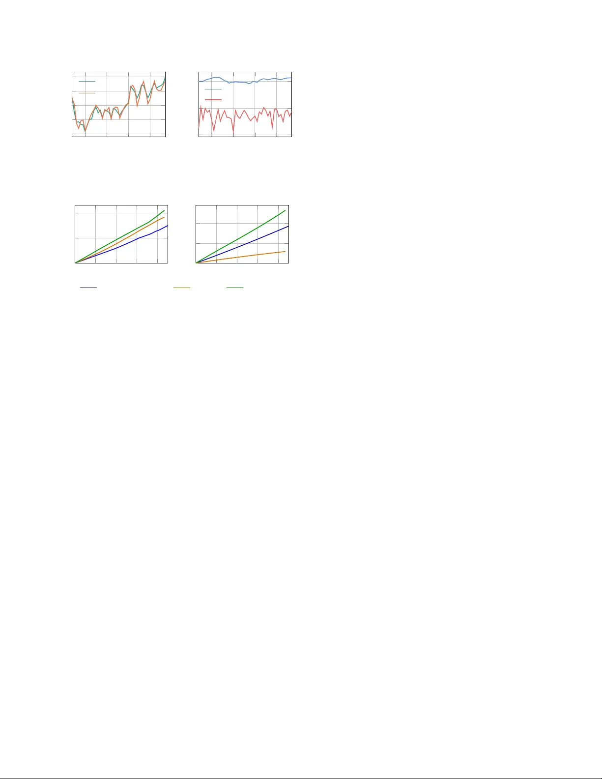
On the Sensitivity of the Subspace Pr edictor to Beha vioral P erturbations Dian Jin, Jeremy Coulson Abstract — Behavioral systems define discrete-time Linear Time-In variant (L TI) systems in terms of a set of trajectories, which forms a linear subspace. This subspace underlies the sub- space predictor used in data-driven prediction and control. In practice, such subspaces are typically represented through data matrices. For rob ustness certification and uncertainty quantifi- cation, howev er , these matrix representations are coordinate- dependent and ther efore do not pr ovide a coordinate-fr ee way to quantify uncertainty . In this work, we establish two key properties of the subspace pr edictor . W e first show that the subspace pr edictor is in variant under change of basis and depends only on the underlying behavioral subspace. W e then derive the first explicit prediction error bound in terms of behavioral distance between the true subspace and an estimate, showing that the predictor is locally Lipschitz with respect to behavioral perturbations. W e also present a one-step prediction error bound that is relev ant for receding-horizon implementations which can be computed directly . Numerical experiments show that the theoretical bound upper-bounds the prediction error , and the a verage prediction error bound gro ws linearly with the beha vioral distance. Index T erms — Behavioral systems, subspace predictor I . I N T RO D U C T I O N Prediction from data is a canonical problem across many areas, including machine learning, signal processing, and control. A common theme across these areas is to extract low-comple xity structure that can be exploited for fore- casting and decision making. In systems and control, this viewpoint has giv en rise to subspace-based methods for system identification [1] and Data-enabled Predictiv e Control (DeePC) [2]. Howe ver , most existing robustness analyses are e xpressed in terms of matrix representations of the data [3], [4], rather than the underlying subspace itself. Consequently , they do not directly address the coordinate- free sensitivity of subspace-based prediction to perturbations. In this work, we study the robustness of subspace prediction under perturbation at the subspace lev el. Behavioral systems theory [5] provides a trajectory-based viewpoint for finite-horizon L TI systems, together with a representation that can be constructed directly from data. This perspectiv e has led to a range of data-driven simulation and control methods [2], [6]–[8]; see [9] and references therein. In particular, data-driven prediction methods utilize an offline data library collected from the system to predict the future output sequence under a prescribed future input sequence. T o accommodate time-varying dynamics, recent works [10], [11] combine subspace prediction [12] with subspace tracking, modeling the e volution of system beha vior Both authors are with the Department of Electrical and Computer Engineering, Uni versity of Wisconsin–Madison, Madison, WI, USA (emails: { djin38, jeremy .coulson } @wisc.edu) as a sequence of varying subspaces. In these approaches, the data matrix is replaced by an orthonormal basis spanning its column space. This shift from representing a behavior through a particular matrix representation to the underlying subspace naturally motiv ates modeling uncertainty directly at the lev el of subspaces. Recent works [10], [13]–[16] hav e adopted this geometric viewpoint, modeling uncertainty sets as collections of subspaces within a fixed distance from a nominal subspace. Howe ver , subspace discrepancy is quantified in subspace distances (e.g., chordal distance [17]), whereas prediction performance is measured in terms of output errors in the Euclidean norm. In particular , it is unclear ho w such geometric discrepancies af fect predicted outputs. Consequently , geometric accuracy of a subspace es- timate does not directly translate into performance guarantees for the resulting predictor . This work bridges this gap. The contribution of this work is twofold. First, we quantify in Theorem 1 the sensitivity of the subspace predictor to behavioral perturbations by deri ving an explicit upper bound on the prediction error in terms of the behavioral distance between the ground-truth subspace and its approximation. The bound also depends on a quantitati ve observ ability property of the system. Second, to support this perturbation analysis, we show in Theorem 2 that the subspace predictor depends only on the subspace spanned by the data matrix, rather than on the particular matrix representation itself. In other words, different data libraries spanning the same underlying subspace lead to the same prediction under the same input. The letter is organized as follo ws: Section II formalizes the problem of interest. Section III contains the main results (Theorem 1 and Theorem 2). Section IV empirically studies the sensitivity of the subspace prediction in terms of the behavioral distance through a numerical case study . Notation: The set of all nonnegati ve integers is denoted Z ≥ 0 . Giv en i, j, T ∈ Z ≥ 0 with i < j and a sequence { z ( t ) } T − 1 t =0 ⊂ R n , define [ i, j ] = [ i, i + 1 , . . . , j − 1 , j ] and z [ i,j ] : = [ z ( i ) ⊤ z ( i + 1) ⊤ · · · z ( j ) ⊤ ] ⊤ . W e use ∥ · ∥ 2 to denote both the Euclidean norm for vectors and the spectral norm for matrices, and ∥ · ∥ F to denote the Frobenius norm. Giv en an integer k ∈ Z ≥ 0 with k ≤ j − i + 1 , define the Hankel matrix of depth k associated with z [ i,j ] as H k  z [ i,j ]  :=      z ( i ) z ( i + 1) · · · z ( j − k + 1) z ( i + 1) z ( i + 2) · · · z ( j − k + 2) . . . . . . . . . . . . z ( i + k − 1) z ( i + k ) · · · z ( j )      . Giv en T ∈ Z ≥ 0 , the sequence z [0 ,T − 1] is called persistently exciting of order k if H k ( z [0 ,T − 1] ) has full row rank. The Moore-Penrose inv erse of a matrix M is denoted by M † . W e use boldface U to denote a linear subspace of R q , and plain U to denote a spanning matrix. These notations are connected by im U = U , and will be used interchangeably . The set of orthogonal matrices is denoted O( d ) = { U ∈ R d × d : U ⊤ U = I } . The set of all singular values of a matrix U is denoted by σ ( U ) . The i th singular value of a matrix U is denoted by σ i ( U ) . The diagonal matrix with diagonal entries γ 1 , · · · , γ d is denoted diag ( γ 1 , · · · , γ d ) . The Grassmannian is defined as Gr( q , d ) : = { U is a linear subspace of R q : dim U = d } . Let U , V ∈ Gr( q , d ) and let U, V ∈ R q × d be orthonormal bases spanning U and V , respectiv ely . Consider the compact singular value decomposition (SVD) U ⊤ V = P Σ Q ⊤ , where Σ = diag( σ 1 , . . . , σ d ) with σ 1 ≥ · · · ≥ σ d ≥ 0 . The principal angles θ 1 , . . . , θ d ∈ [0 , π / 2] between U and V are giv en by [18] cos θ i = σ i . The chor dal distance between U , V is defined equi valently by d ( U , V ) = d X i =1 sin 2 θ i ! 1 2 = 1 √ 2   U U ⊤ − V V ⊤   F . (1) Note that the chordal distance is representation free: d (im ( U Q ) , im ( V Q )) = d (im U, im V ) for all Q ∈ O( d ) . The Gaussian distribution with mean 0 and covariance Σ ∈ R d × d is denoted N (0 , Σ) . I I . P RO B L E M S TA T E M E N T Consider the observable L TI dynamical system x ( t + 1) = Ax ( t ) + B u ( t ) , y ( t ) = C x ( t ) + Du ( t ) , (2) where A ∈ R n × n , B ∈ R n × m , C ∈ R p × n , D ∈ R p × m , x ( t ) is the state, u ( t ) is the input, y ( t ) is the output at time t ∈ Z ≥ 0 . The r estricted behavior of (2) is defined as B [0 ,L − 1] =   u [0 ,L − 1] , y [0 ,L − 1]  ∈ R ( m + p ) L     there exists x [0 ,L ] ∈ R n ( L +1) such that (2) holds for all t ∈ [0 , L − 1]  . Any ( u [0 ,L − 1] , y [0 ,L − 1] ) ∈ B [0 ,L − 1] is called a trajectory of system (2). The following lemma [9] shows that B [0 ,L − 1] is a linear subspace of R ( m + p ) L and provides a data matrix representation. Lemma 1 ( [19, Corollary 19]) . Consider system (2) . Let ( A, B ) be contr ollable and L ≥ n . Then B [0 ,L − 1] is a linear subspace of dimension dim B [0 ,L − 1] = mL + n . Mor eover , let T ∈ Z > 0 and ( u [0 ,T − 1] , y [0 ,T − 1] ) ∈ B [0 ,L − 1] with u [0 ,T − 1] being persistently exciting of order n + L , then im  H L ( u [0 ,T − 1] ) H L ( y [0 ,T − 1] )  = B [0 ,L − 1] . Lemma 1 provides the foundation for viewing systems over finite horizons as subspaces [15]. The data-dri ven prediction problem posed in [6] aims to find the output sequence of an unknown dynamical system corresponding to an input sequence based on a past input-output trajectory collected from the system, without explicitly identifying a state-space model. W e now introduce the subspace predictor , which is the key ingredient of data-driv en prediction and the main object studied in this work. Definition 1. Let X ∈ R ( m + p )( T ini + T f ) × r , r ∈ Z > 0 . Let ( u ini , u, y ini ) ∈ R mT ini + mT f + pT ini . P artition X into a block matrix X =  X ⊤ u p X ⊤ u f X ⊤ y p X ⊤ y f  ⊤ , wher e X u p ∈ R mT ini × r , X u f ∈ R mT f × r , X y p ∈ R pT ini × r , X y f ∈ R pT f × r . The subspace pr edictor is defined as the mapping S : R ( m + p )( T ini + T f ) × r × R mT ini + mT f + pT ini → R pT f , S ( X , u ini , u, y ini ) = X y f   X u p X u f X y p   †   u ini u y ini   . (3) Throughout this paper, the subscripts u p , u f , y p , y f always refer to this block partition for any matrices with ( m + p )( T ini + T f ) rows. When the vector ( u ini , u, y ini ) is clear from the context, we equiv alently write y pred [0 ,T f − 1] ( X ) : = ( y pred 0 ( X ) , . . . , y pred T f − 1 ( X )) for S ( X , u ini , u, y ini ) . The sub- space predictor can be used to predict future output trajecto- ries of a dynamical system giv en future input u ∈ R mT f and an initial trajectory ( u ini , y ini ) ∈ B [0 ,T ini − 1] [6]. W e wish to study ho w the perturbation to B [0 ,T ini + T f − 1] affects the subspace prediction. Let b B [0 ,T ini + T f − 1] be the behavior of an approximate system b x ( t + 1) = b A b x ( t ) + b B u ( t ) , b y ( t ) = b C b x ( t ) + b D u ( t ) , (4) where b A ∈ R n × n , b B ∈ R n × m , b C ∈ R p × n , b D ∈ R p × m . Let u d [0 ,T − 1] be persistently exciting of order n + T ini + T f , let ( u d [0 ,T − 1] , y d [0 ,T − 1] ) ∈ B [0 ,T ini + T f − 1] and ( u d [0 ,T − 1] , b y d [0 ,T − 1] ) ∈ b B [0 ,T ini + T f − 1] . W e arrange them into Hankel matrices H : = " H T ini + T f ( u d [0 ,T − 1] ) H T ini + T f ( y d [0 ,T − 1] ) # , b H : = " H T ini + T f ( u d [0 ,T − 1] ) H T ini + T f ( b y d [0 ,T − 1] ) # . (5) Giv en ( u ini , y ini ) ∈ B [0 ,T ini − 1] and an input sequence u ∈ R mT f , we denote the predicted output sequence as- sociated with these Hankel matrices by y pred [0 ,T f − 1] ( H ) and y pred [0 ,T f − 1] ( b H ) . Note that ( u ini , y ini ) need not be a T ini - length trajectory of (4), since the subspace predictor S is defined for arbitrary ( u ini , y ini ) ∈ R ( m + p ) T ini . This corre- sponds to the practical setting in which the approximate subspace, b B [0 ,T ini + T f − 1] , is used for prediction. Denote b = ( u ini , u, y ini ) . Denote M = [ H ⊤ u p H ⊤ u f H ⊤ y p ] ⊤ and similar for c M , the prediction error can be first bounded as    y pred [0 ,T f − 1] ( b H ) − y pred [0 ,T f − 1] ( H )    2 ≤     b H y f    2    c M † − M †    2 +    b H y f − H y f    F   M †   2  ∥ b ∥ 2 ≤     b H y f    2    c M † − M †    2 +    b H − H    F   M †   2  ∥ b ∥ 2 , (6) where the last inequality uses the fact that b H y f and H y f are Fig. 1: The two planes represent the nominal restricted behavior U and its approximation b U , with discrepancy measured by d ( b U , U ) . submatrices of b H and H , respectively . Ho wever , the bound in (6) is still expressed in terms of matrix norms. As such, it is not intrinsic to the underlying restricted behaviors, and the bound may vary under different matrix representations of the same subspace. Since our goal is to relate prediction error to a geometric discrepancy between restricted behaviors, it is natural to seek a representation-free bound formulated directly in terms of d (im b H , im H ) , see Fig. 1. Because each restricted behavior is a linear subspace by Lemma 1, we use chordal distance d to measure discrep- ancy between restricted behaviors, and will refer to chordal distance and beha vioral distance interchangeably . This gives rise to the central question of this letter: Problem 1. How do perturbations measur ed in chor dal distance between r estricted behaviors affect the subspace pr ediction? Mor e pr ecisely , how can the prediction err or    y pred [0 ,T f − 1] ( H ) − y pred [0 ,T f − 1] ( b H )    2 be bounded in terms of d (im H , im b H ) ? W e address this problem in Section III. W e first examine how observability properties of (2) af fect the prediction error bound giv en by (8), then we show that the subspace predictor S is coordinate-free (Theorem 2). Finally , we relate the Frobenius norm to behavioral distance through a suitable basis representation (Lemma 3), which leads to a nov el prediction error bound (Theorem 1). I I I . P R E D I C T I O N E R RO R B O U N D W e introduce a state-space formulation of the restricted behavior . For k ∈ Z ≥ 0 , define the extended observability matrix and block T oeplitz matrix as O k =      C C A . . . C A k − 1      , T k =      D 0 · · · 0 C B D · · · 0 . . . . . . . . . . . . C A k − 2 B C A k − 3 B · · · D      . Let ( u [0 ,L − 1] , y [0 ,L − 1] ) ∈ B [0 ,L − 1] with corresponding state sequence x [0 ,L ] . Denote Φ L : =  0 I mL O L T L  , then  H L  u [0 ,T − 1]  H L  y [0 ,T − 1]   = Φ L  H 1  x [0 ,T − L ]  H L  u [0 ,T − 1]   . (7) It is shown in [19, Corollary 19] that im Φ L = B [0 ,L − 1] . W e refer to Φ L as the trajectory generation matrix of (2). The main theorem below assumes a lower bound on σ min (Φ L ) , a quantity tied to the observ ability property of (2), which is analyzed in Section III-A. W e now state the main theorem. Theorem 1 (Local Lipschitz continuity of the subspace predictor) . Consider system (2) . Let T ini , T f ∈ Z > 0 and let T ini ≥ n . Let Φ T ini and Φ T ini + T f be trajectory generation matrices of (2) . Suppose there exists β > 0 such that σ min (Φ T ini ) ≥ β and let σ max (Φ T ini + T f ) = α > 0 . Let ( u ini , y ini ) ∈ B [0 ,T ini − 1] , u ∈ R mT f . Let H and b H satisfy B [0 ,T ini + T f − 1] = im H and b B [0 ,T ini + T f − 1] = im b H . Denote γ = min(1 , β ) /α , if d (im b H , im b H ) ≤ γ / 2 √ 2 , then    y pred [0 ,T f − 1] ( b H ) − y pred [0 ,T f − 1] ( H )    2 ≤ 2(1 + √ 5) γ 2 + 1 γ ! √ 2 d (im b H , im H ) ∥ ( u ini , u, y ini ) ∥ 2 . (8) Theorem 1 answers Problem 1 by quantifying how per- turbations of restricted behavior , measured in beha vioral distance, affect the prediction error . In particular, the bound in (8) is representation-free: it depends only on the restricted behaviors im b U and im U , and not on the particular ma- trix representations. This shows that sensitivity of subspace prediction can be characterized at the geometric le vel. The proof of Theorem 1, presented in Section III-D, relies on three auxiliary results, dev eloped in the following sections. A. On the quantitative observability condition W e no w turn to the assumption on σ min (Φ T ini ) in Theorem 1. The follo wing proposition shows that this assumption is equiv alent to observability of system (2). Proposition 1. Let T ini ≥ n . Then there exists β > 0 such that σ min (Φ T ini ) ≥ β if and only if rank( O T ini ) = n. Pr oof. Positivity of σ min (Φ T ini ) implies that Φ T ini has full column rank n + mT ini . The upper right block I mT ini has rank mT ini , so the remaining n columns must be linearly indepen- dent, which is equiv alent to rank( O T ini ) = n . Con versely , if rank( O T ini ) = n , then the structure of Φ T ini implies that Φ T ini has full column rank, and hence σ min (Φ T ini ) > 0 . This viewpoint also aligns with the quantitativ e observability condition [20, Eq. (20)] introduced in the robust fundamental lemma, which assumes a lower bound on σ min (Φ T ini + T f ) . The parameter β quantifies the de gr ee of observ ability . Lemma 2. Consider system (2) . Let T ini ≥ n , T f ∈ Z > 0 . Let V ∈ R ( m + p )( T ini + T f ) × r be an orthonormal basis of im Φ T ini + T f . Denote M = [ V ⊤ u p V ⊤ u f V ⊤ y p ] ⊤ . Assume that σ min (Φ T ini ) ≥ β for some β > 0 and σ max (Φ T ini + T f ) = α > 0 . Then M satisfies σ min ( M ) ≥ min { 1 , β } /α. The bound is also r epr esentation-free in the sense that σ min ( M P ) ≥ min { 1 , β } /α for all P ∈ O( r ) . Pr oof. Let U be the orthonormal matrix from the QR fac- torization Φ T ini + T f = U R , where R is inv ertible. Then there exists Q ∈ O( r ) such that U = V Q . Let Π denote the operator that selects the first mT ini + mT f + pT ini rows of a matrix such that M = Π V = Π U Q . Then ΠΦ T ini + T f = (Π V Q ) R = M QR. The matrix ΠΦ T ini + T f admits the form ΠΦ T ini + T f =   0 I mT ini 0 0 0 I mT f O T ini T T ini 0   : =  F | G  where F =   0 I mT ini 0 0 O T ini T T ini   and G =   0 I mT f 0   . Since F ⊤ G = 0 , the column spaces of F and G are orthog- onal. Therefore for any vector x = ( x 1 , x 2 ) where x 1 ∈ R mT ini + pT ini , x 2 ∈ R mT f , ∥ ΠΦ T ini + T f x ∥ 2 2 = ∥ F x 1 ∥ 2 2 + ∥ Gx 2 ∥ 2 2 ≥ σ min ( F ) 2 ∥ x 1 ∥ 2 2 + σ min ( G ) 2 ∥ x 2 ∥ 2 2 ≥ min( σ min ( F ) 2 , σ min ( G ) 2 )( ∥ x 1 ∥ 2 2 + ∥ x 2 ∥ 2 2 ) = min( σ min ( F ) 2 , σ min ( G ) 2 ) ∥ x ∥ 2 2 . Now σ min ( G ) = 1 , and σ min ( F ) = σ min (Φ T ini ) ≥ β . There- fore, σ min (ΠΦ T ini + T f ) ≥ min { β , 1 } . W e have the inequality ∥ X Y x ∥ 2 ≥ σ min ( X ) ∥ Y x ∥ 2 ≥ σ min ( X ) σ min ( Y ) ∥ x ∥ 2 for all x ∈ R r , where X = ΠΦ T ini + T f , Y = ( QR ) − 1 . Hence σ min ( X Y ) ≥ σ min ( X ) σ min ( Y ) . Since Φ T ini + T f has full column rank and R is inv ertible, σ min ( M ) = σ min ( X Y ) ≥ σ min ( X ) σ min (( QR ) − 1 ) = σ min (ΠΦ T ini + T f ) /σ max ( QR ) = σ min (ΠΦ T ini + T f ) /σ max ( R ) ≥ min { 1 , β } /α. Finally , since σ ( M P ) = σ ( M ) for all P ∈ O( r ) , we hav e σ min ( M P ) = σ min ( M ) . Denote γ = min(1 , β ) /α , then we see that the bound in Theorem 1 improv es as β increases, and deteriorates as α increases. In this sense, a system with stronger quantitativ e observability leads to a tighter bound, while a larger gain α leads to greater sensitivity to behavioral perturbations. B. Repr esentation-free subspace predictor W e establish that the subspace predictor depends only on the restricted behavior , rather than on the particular matrix representation. Theorem 2. Let T ini , T f ∈ Z > 0 . Let X, Y ∈ R ( m + p )( T ini + T f ) × r , r ∈ Z > 0 . Suppose im X = im Y . Assume M = [ X ⊤ u p X ⊤ u f X ⊤ y p ] ⊤ has full column rank. Then for any b : = ( u ini , u, y ini ) ∈ R m ( T ini + T f )+ pT ini , S ( X , u ini , u, y ini ) = S ( Y , u ini , u, y ini ) . Pr oof. Since M has full column rank and M is a submatrix of X , we ha ve rank X = rank Y = r . Consider the QR decompositions [18, Theorem 5.2.3] X = U R X , Y = V R Y , where U, V ∈ R ( m + p )( T ini + T f ) × r are orthonormal and R X , R Y ∈ R r × r are in vertible. Since im X = im Y , we have im U = im V , hence V = U Q for some Q ∈ O( r ) . Denote M U = [ U ⊤ u p U ⊤ u f U ⊤ y p ] ⊤ , then M = M U R X , which implies M U also has full column rank. Then ( M U R X ) † = R − 1 X M † U . Therefore, y pred [0 ,T f − 1] ( X ) = ( U y f R X )( M U R X ) † b = U y f R X ( R − 1 X M † U ) b = U y f M † U b. Similarly , we have y pred [0 ,T f − 1] ( Y ) = U y f QR Y ( M U QR Y ) † b = U y f QR Y R − 1 Y ( M U Q ) † b = U y f QQ ⊤ M † U b = U y f M † U b. Thus y pred [0 ,T f − 1] ( X ) = y pred [0 ,T f − 1] ( Y ) . Theorem 2 implies that S can be viewed as a well-defined mapping on the Grassmannian, i.e., S : Gr(( m + p )( T ini + T f ) , r ) × R m ( T ini + T f )+ pT ini → R pT f , S ( U , u ini , u, y ini ) = U y f   U u p U u f U y p   †   u ini u y ini   , where U is an orthonormal basis of U . When the vector ( u ini , u, y ini ) is clear from context, the notations S ( U ) , S ( U ) , y pred [0 ,T f − 1] ( U ) will be used interchangeably . No w we can replace H and b H in (6) with their orthonormal bases U and b U , respectively . Then (6) re veals two sources of prediction error: one through the sensitivity of M † , gov erned by the singular values of M , and the other is related to the matrix norm ∥ b U − U ∥ F which depends on the basis representations of the restricted behaviors im b H and im H . W e next study the quantitative observability of (2), which is related to the magnitude of the singular values of M . C. Basis alignment and chor dal distance The term ∥ b U − U ∥ F in (6) depends on the particular choice of basis of b U and U , whereas the prediction error    y pred [0 ,T f − 1] ( b U ) − y pred [0 ,T f − 1] ( U )    2 remains in variant by Theo- rem 2. It is therefore natural to choose orthonormal bases that minimize ∥ b U − U ∥ F . The following lemma is classical and closely related to the orthogonal Procrustes problem [21]. W e include it here for completeness, since the proof highlights the geometric role of principal angles and aligns with the subspace-based viewpoint adopted in this work. Lemma 3. Let U , b U ∈ Gr(( m + p ) L, r ) with orthonormal bases U and b U , r espectively . Let θ 1 , . . . , θ r be the principal angles between U and b U . Then min R ∈ O( r )    U − b U R    2 F = 2 r − 2 r X i =1 cos θ i . The minimum is attained at R ∗ = QP ⊤ , wher e U ⊤ b U = P cos Θ Q ⊤ is the compact SVD with cos Θ : = diag(cos θ 1 , . . . , cos θ r ) . In particular ,    U − b U R ∗    F ≤ √ 2 d ( U , b U ) . Pr oof. Let R ∈ O( r ) , we have ∥ U − b U R ∥ 2 F = 2 r − 2 T r( U ⊤ b U R ) . Denoting S = Q ⊤ RP , we hav e T r  U ⊤ b U R  = T r  P cos Θ Q ⊤ R  = T r(cos Θ S ) = r X i =1 S ii cos θ i . Since S = Q ⊤ RP ∈ O( r ) , we hav e | S ii | ≤ 1 for i = 1 , . . . , r . Therefore, T r( U ⊤ b U R ) is maximized when R = QP ⊤ , in which case S = I r . Then    U − b U QP ⊤    2 F = 2 r − 2 r X i =1 cos θ i ≤ 2 r X i =1 sin 2 θ i = 2 d ( b U , U ) 2 , where we use the inequality 1 − cos θ i ≤ sin 2 θ i , which follows from sin 2 θ i − (1 − cos θ i ) = cos θ i (1 − cos θ i ) ≥ 0 for all θ i ∈ [0 , π / 2] . D. Pr oof of Theorem 1 By Lemma 3, once an orthonormal basis U of U = im H is fixed, we may choose an orthonormal basis b U of b U = im b H so that ∥ b U − U ∥ F is minimized. In the following, b U denotes such a minimizing basis constructed in Lemma 3. Denote κ = d ( b U , U ) , we ha ve ∥ b U y f − U y f ∥ F ≤ ∥ b U − U ∥ F ≤ √ 2 κ . The difference between c M † and M † can be bounded using results on perturbation of pseudo-in verse [22, Theorem 3.3], which implies    c M † − M †    2 ≤ 1 + √ 5 2 max     c M †    2 2 ,   M †   2 2     c M − M    2 . By W eyl’ s inequality [23, Eq. (3.3.19)] for singular values and Lemma 3, | σ min ( c M ) − σ min ( M ) | ≤    c M − M    2 ≤    c M − M    F ≤ √ 2 κ, hence σ min ( c M ) ≥ σ min ( M ) − √ 2 κ ≥ γ − √ 2 κ by Lemma 2. Since κ ≤ γ / 2 √ 2 , then σ min ( c M ) ≥ γ / 2 , so ∥ c M † ∥ 2 = σ min ( c M ) − 1 ≤ 2 /γ . W e then hav e max     c M †    2 2 ,   M †   2 2  ≤ max  4 γ 2 , 1 γ 2  = 4 γ 2 , Plugging the abo ve inequalities into (6), using Lemma 3, and using the fact that ∥ b U y f ∥ 2 ≤ ∥ b U ∥ 2 = 1 , we have    S ( b H ) − S ( H )    2 =    S ( b U ) − S ( U )    2 ≤ 2(1 + √ 5) ∥ b U y f ∥ 2 γ 2 + 1 γ !    b U − U    F ∥ b ∥ 2 ≤ 2(1 + √ 5) γ 2 + 1 γ ! √ 2 d ( b U , U ) ∥ b ∥ 2 . (9) E. One-step pr ediction err or bound In many predictive control methods, only the first pre- dicted output is used at each step. In this case, a bound on the one-step prediction error is more rele vant than a bound on the full T f -step prediction error . The remaining non-computable term is d ( b U , U ) , which depends on the unknown ground- truth subspace U . In concrete applications such as online system identification, this quantity can be upper bounded by computable terms; see [10] for details. On the other hand, c M is constructed from the estimated subspace and is therefore computable. This motiv ates a reformulation of the prediction error bound in terms of σ min ( c M ) , yielding a fully data- dependent and practically verifiable condition. Corollary 1. Let b U (1) y f : = [ I p 0 · · · 0] b U y f which is the first p r ows of b U y f . Under the assumption of Theorem 1, except that the condition κ ≤ γ / (2 √ 2) is replaced by κ ≤ σ min ( c M ) / (2 √ 2) , and assuming σ min ( c M ) > 0 , we have    y pred 0 ( b U ) − y pred 0 ( U )    2 ≤ 2(1 + √ 5) ∥ b U (1) y f ∥ 2 σ min ( c M ) 2 + 1 σ min ( c M ) ! √ 2 d ( b U , U ) ∥ b ∥ 2 . (10) Pr oof. Similar to (6), we also have    y pred 0 ( b U ) − y pred 0 ( U )    2 ≤  ∥ H y f ∥ 2    M − c M †    2 +    b H y f − H y f    F    c M †    2  ∥ b ∥ 2 . By W eyl’ s inequality used in Section III-D, we ha ve σ min ( M ) ≥ σ min ( c M ) − √ 2 κ ≥ σ min ( c M ) / 2 , so that ∥ M † ∥ 2 = σ min ( M ) − 1 ≤ 2 /σ min ( c M ) . Therefore, max {∥ M † ∥ 2 2 , ∥ c M † ∥ 2 2 } ≤ 4 /σ min ( c M ) 2 . The rest of the proof proceeds similarly as in Section III-D, which yields the bound (10). I V . N U M E R I C A L E X P E R I M E N T W e illustrate the theoretical results on a L TI system 1 . The goal is to explore the relationship between beha vioral pertur- bations and the prediction error bound. Consider system (2) with A =  0 . 8 0 . 2 0 . 1 0 . 9  , B = [0 . 3 0 . 7] ⊤ , C = [1 1] , D = 0 . The initial state is set to x 0 = 0 ∈ R 2 . The true subspace U is constructed via offline Hankel data collection: Let ( u d [0 ,T − 1] , y d [0 ,T − 1] + η d [0 ,T − 1] ) be an offline trajectory of system (2), where η d t ∈ N (0 , σ ∥ y d t ∥ 2 2 I p ) with σ = 0 . 02 being the noise-to-signal ratio, where u d [0 ,T − 1] is persistently exciting of order n + T ini + T f . W e vary ( T ini , T f ) ov er { (4 , 4) , (4 , 2) , (2 , 4) } and set T = 30 . W e org anize the offline data into a L -depth Hankel matrix H defined by (5), where L = T ini + T f . W e obtain an orthonormal basis U ∈ R ( m + p ) L × r of the subspace im H through SVD. In this experiment we choose r = mL + n , which is the dimension of the restricted behavior of (2) by Lemma 1. W e generate a family of perturbed subspaces { b U n } N n =1 with N = 100 . W e fix an input sequence u [0 ,T sim − 1] , and let y [0 ,T sim − 1] + η [0 ,T sim − 1] to be the measured output from system (2), where T sim = 50 , y [0 ,T sim − 1] is the noise-free output sequence and η t ∈ N (0 , σ ∥ y t ∥ 2 2 I p ) . For each fixed b U n , the T f -length prediction at t ∈ [ T ini , T end ] (denote T end : = T sim − T f + 1 ) is given by S ( b U n , u [ t − T ini ,t − 1] , y [ t − T ini ,t − 1] + η [ t − T ini ,t − 1] , u [ t,t + T f − 1] ) , and we only keep the first component, denoted by y pred t ( b U n ) . For each b U n , this yields a sequence of one-step predictions y pred [ T ini ,T end ] ( b U n ) . W e compare these with the baseline predic- 1 The code is available at github.com/DianJin- Frederick/sub space_prediction_under_behavioral_perturbation 10 20 30 40 − 4 − 2 0 2 4 Predicted output U b U 100 10 20 30 40 10 − 2 10 0 10 2 Prediction error and bound Error bound Prediction error Fig. 2: Single experiment for T ini = 4 , T f = 2 . The left panel shows the predicted outputs generated by U and b U 100 with κ 100 = 0 . 8680 . The right panel compares the corresponding prediction error and the theoretical bound (10). The horizontal axis sho ws the time indices [ T ini , T end ] . 0 0 . 2 0 . 4 0 . 6 0 . 8 0 0 . 2 0 . 4 A verage prediction error ( T ini , T f ) = (4 , 4) (4 , 2) (2 , 4) 0 0 . 2 0 . 4 0 . 6 0 . 8 200 400 A verage error bound Chordal distance κ Chordal distance κ Fig. 3: A verage prediction error and average prediction error bound (v ertical axis) as functions of the chordal distance for three ( T ini , T f ) . tions y pred [ T ini ,T end ] ( U ) and compute the prediction error e ( n ) t = ∥ y pred t ( b U n ) − y pred t ( U ) ∥ 2 , t ∈ [ T ini , T end ] , and the bound given by (10). W e compute the av erage pre- diction error and bound over [ T ini , T end ] . These quantities are plotted against the chordal distance κ n = d ( b U n , U ) . Fig. 2 illustrates an experiment for b U 100 with κ 100 = 0 . 8680 . The theoretical error bound correctly upper-bounds the prediction error at all t . Fig. 3 summarizes the dependence of prediction errors and bounds on the chordal distance. In all choices of ( T ini , T f ) , the av erage prediction error and bound grow approximately linearly with κ . W e observe that a smaller T f leads to a less demanding prediction task and hence a smaller prediction error . In contrast, a smaller T ini provides less past information, which leads to larger prediction errors and larger bounds. This is in line with the dependence of the bound on the degree of observ ability , β . Despite being conservati ve, we empirically observe that the bound captures the linear growth rate of the prediction error in terms of the behavioral distance. V . C O N C L U S I O N This work shows two fundamental properties of the sub- space predictor . First, we sho wed that it is representation- free, in the sense that it depends only on the restricted be- havior of a system. Second, we derived an explicit prediction error bound directly in terms of the chordal distance between two restricted behaviors. This provides a quantitativ e link between geometric uncertainty and prediction accuracy . Fu- ture work includes combining the results with computable subspace-tracking bounds, and extending the analysis from prediction to closed-loop data-driv en control. W e hope that the representation-free vie wpoint dev eloped will serve as a useful building block for more data-driv en control methods. A C K N O W L E D G E M E N T The authors used ChatGPT to assist with language refine- ment and editing in parts of this manuscript. All generated content was subsequently revie wed and edited by the authors, who take full responsibility for the final manuscript. R E F E R E N C E S [1] P . V an Overschee and B. De Moor, Subspace identification for linear systems: Theory—Implementation—Applications . Springer Science & Business Media, 2012. [2] J. Coulson, J. L ygeros, and F . D ¨ orfler , “Data-enabled predictive control: In the shallo ws of the DeePC, ” in 2019 18th Eur opean control confer ence (ECC) . IEEE, 2019, pp. 307–312. [3] J. Berberich, J. K ¨ ohler , M. A. M ¨ uller , and F . Allg ¨ ower , “Data-driven model predictive control with stability and robustness guarantees, ” IEEE transactions on automatic control , vol. 66, no. 4, pp. 1702– 1717, 2020. [4] C. De Persis and P . T esi, “Formulas for data-driv en control: Stabi- lization, optimality , and rob ustness, ” IEEE T ransactions on A utomatic Contr ol , vol. 65, no. 3, pp. 909–924, 2019. [5] J. C. W illems, “From time series to linear system—Part I. Finite dimensional linear time inv ariant systems, ” Automatica , vol. 22, no. 5, pp. 561–580, 1986. [6] I. Markovsky and P . Rapisarda, “Data-driven simulation and control, ” International Journal of Control , v ol. 81, no. 12, pp. 1946–1959, 2008. [7] J. Coulson, J. L ygeros, and F . D ¨ orfler , “Distributionally rob ust chance constrained data-enabled predictive control, ” IEEE T ransactions on Automatic Contr ol , vol. 67, no. 7, pp. 3289–3304, 2021. [8] F . D ¨ orfler , J. Coulson, and I. Marko vsky , “Bridging direct and indirect data-driv en control formulations via regularizations and relaxations, ” IEEE Tr ansactions on Automatic Contr ol , vol. 68, no. 2, pp. 883–897, 2022. [9] I. Markovsky and F . D ¨ orfler , “Behavioral systems theory in data-dri ven analysis, signal processing, and control, ” Annual Revie ws in Contr ol , vol. 52, pp. 42–64, 2021. [10] A. Sasfi, A. Padoan, I. Markovsk y , and F . D ¨ orfler , “Great: Grassman- nian recursive algorithm for tracking & online system identification, ” IEEE T ransactions on Automatic Contr ol , p. 11267272, 2026. [11] D. Jin and J. Coulson, “Online subspace learning on flag manifolds for system identification, ” arXiv preprint , 2025. [12] W . Fa voreel, B. De Moor, and M. Gev ers, “SPC: Subspace predicti ve control, ” IF AC Proceedings V olumes , vol. 32, no. 2, pp. 4004–4009, 1999. [13] A. Fazzi and I. Markovsky , “Distance problems in the behavioral setting, ” European Journal of Contr ol , vol. 74, p. 100832, 2023. [14] A. Padoan, J. Coulson, H. J. van W aarde, J. L ygeros, and F . D ¨ orfler , “Behavioral uncertainty quantification for data-driven control, ” in 2022 IEEE 61st Conference on Decision and Contr ol (CDC) , 2022, pp. 4726–4731. [15] A. Padoan and J. Coulson, “Distances between finite-horizon linear behaviors, ” IEEE Contr ol Systems Letters , 2025. [16] S. Bharadwaj, B. Mishra, C. Mostajeran, A. Padoan, J. Coulson, and R. N. Banavar , “Robust least-squares optimization for data- driv en predictive control: A geometric approach, ” arXiv preprint arXiv:2511.09242 , 2025. [17] K. Y e and L.-H. Lim, “Schubert varieties and distances between subspaces of different dimensions, ” SIAM Journal on Matrix Analysis and Applications , vol. 37, no. 3, pp. 1176–1197, 2016. [18] G. H. Golub and C. F . V an Loan, Matrix computations . JHU press, 2013. [19] I. Marko vsky and F . D ¨ orfler , “Identifiability in the behavioral setting, ” IEEE T ransactions on Automatic Contr ol , vol. 68, no. 3, pp. 1667– 1677, 2022. [20] J. Coulson, H. J. V an W aarde, J. L ygeros, and F . D ¨ orfler , “ A quanti- tativ e notion of persistency of excitation and the robust fundamental lemma, ” IEEE Contr ol Systems Letters , vol. 7, pp. 1243–1248, 2022. [21] P . H. Sch ¨ onemann, “ A generalized solution of the orthogonal pro- crustes problem, ” Psychometrika , vol. 31, no. 1, pp. 1–10, 1966. [22] G. W . Stew art, “On the perturbation of pseudo-inv erses, projections and linear least squares problems, ” SIAM re view , vol. 19, no. 4, pp. 634–662, 1977. [23] H. Roger and R. J. Charles, “T opics in matrix analysis, ” 1994.