Collapsing Flat ${\rm{SU}}(2)$-Bundles to Spherical 3-Manifolds

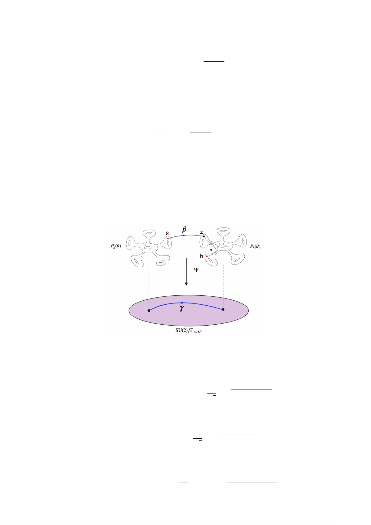
Collapsing Flat SU(2) -Bundles to Spherical 3 -Manifolds Eder M. Cor rea 1 1 Univ ersidade Estadual de Campinas, Brazil, Instituto de Matemática, Estatística e Computação Científica, ederc@unicamp.br March 19, 2026 Abstr act W e present a geometric mechanism f or the emergence of spherical 3 -manifolds fr om the super- space of Riemannian metrics associated with flat SU(2) -bundles o ver closed or ientable hyperbolic surfaces. Our main result show s t hat any spherical 3-manifold ( 𝑆 , 𝑔 𝑆 ) can be realized as a boundar y point in the Gromov -Hausdor ff closure of a superspace  ( 𝑃 ) , where 𝑃 is a flat SU(2) -bundle over a closed or ientable hyperbolic surface (Σ , ℎ Σ ) . W e show that t he conv ergence of the sequence of metric spaces tow ards the spher ical limit is controlled by the order of the fundamental group of 𝑆 and the metric invariant of the hyperbolic base pro vided by the ratio between its area and its systole. In this framew ork, the problem of obtaining the shar pest upper bound er ror reduces to the classical problem of maximizing the systole function o ver t he moduli space of hyperbolic Riemann sur faces. As a byproduct, w e obser ve that certain ar ithmetic surfaces pro vide the best possible er ror estimates within this famil y . T o illustrate these results, we show t hat, according to our mechanism, the Bolza surface yields the optimal er ror bound for the con verg ence tow ard the Poincaré homology sphere. Contents 1 Introduction 1 2 Generalities on Hyperbolic Surfaces 5 3 Flat Principal Bundles 6 4 Spherical 3-manifolds and Flat SU(2) -bundles 10 5 Gromo v-Hausdorff Space 13 6 Superspace of Riemannian Metrics 14 7 Proof of Main Result 15 8 From Bolza Surface to Poincaré Homology Sphere 17 1 Introduction The ADE diagrams first appeared in Coxe ter’ s classification of reflection-generated finite g roups in the 1930s, e.g. [ Cox34 ]. They reappeared a decade later in Dynkin ’ s classification of semisimple Lie alge- bras, see [ Dyn47 ]. Since the 1970s, these same diagrams hav e continued to surface across mathematics and physics, from representation theor y and algebraic geome tr y to quiv er theor y and gaug e theor y . For a comprehensiv e account of this ubiquitous and intr iguing patter n, we refer the reader to [ CDHM25 ]. ⋯ (a) 𝐴 𝑛 ⋯ (b) 𝐷 𝑛 (c) 𝐸 6 (d) 𝐸 7 (e) 𝐸 8 Figure 1: ADE type Dynkin diagrams. 1 A par ticularly notable instance is the McKa y correspondence [ McK80 ], which establishes a direct link be tween the finite subgroups of SU(2) , the binary pol yhedral groups, and the ADE diagrams. These groups, namely the cyclic, binar y dihedral, binary tetrahedral, binary octahedral, and binary icosahedral groups, are t he building blocks f or some of t he most symmetric geometric objects in t hree dimensions. Figure 2: The symmetry groups of the Platonic solids cor respond, via the McKa y cor respondence, to the ex ceptional Dynkin diagrams 𝐸 6 , 𝐸 7 , and 𝐸 8 of the ADE classification [ Dec18 ]. In Riemannian geometry , t he significance of these g roups is realized through the spher ical 3 -manifolds. By the Killing-Hopf t heorem [ W ol11 , §2.4], a complete, simply connected Riemannian manifold of constant positive cur vature +1 is isometric to the 3 -sphere 𝑆 3 ≅ SU(2) . Consequentl y , any closed orient able spherical 3 -manif old is isometric to a quotient SU(2)∕Γ 𝐴𝐷𝐸 , where Γ 𝐴𝐷𝐸 ⊂ SU(2) is a finite subgroup and therefore one of the binary polyhedral groups from the ADE list [ Sco83 ], [ Mil75 ]. These manif olds f or m a cr ucial class within Thurston ’ s geometrization prog ram [ Thu22b ], [ Thu22a ]. The geometrization conjecture, prov en by Perelman [ Per02 , Per03b , Per03a ], asser ts that ev er y closed 3 - manif old can be decomposed into pieces, each admitting one of eight geometric structures. The spherical manif olds are precisely those that admit a metric of constant positive curvature, ser ving as the most symmetric models in this classification. In a parallel de velopment, flat SU(2) -bundles o ver closed surfaces ( 𝑔 > 1 ) ha ve become a central object of study in differential geome try and mat hematical physics, e.g. [ Hit87 ], [ AB83 ], [ Sen98 ]. By the Riemann-Hilbert correspondence, these bundles are classified by conjugacy classes of representations of the surface’ s fundamental g roup into SU(2) , see f or instance [ Tau11 , Chap. 13]. The resulting moduli space  flat (Σ , SU(2)) , giv en b y  flat (Σ , SU(2)) ≅ Hom( 𝜋 1 (Σ) , SU(2))∕SU(2) , (1.1) is a finite-dimensional singular symplectic space, whose geometry is deepl y intertwined with gauge theor y , integrable systems, and geometric quantization, see f or instance [ Dey06 ] and ref erences t herein. In the abov e setting, for every ADE subgroup Γ 𝐴𝐷𝐸 ⊂ SU(2) , we can construct a flat principal SU(2) - bundle 𝑃 → Σ 𝑔 ( 𝑔 > 1 ) equipped with a principal flat connection 𝜃 ∈ Ω 1 ( 𝑃 , 𝔰𝔲 (2)) , such that Hol( 𝜃 ) ≅ Γ 𝐴𝐷𝐸 . (1.2) The principal flat SU(2) -bundle ( 𝑃 , 𝜃 ) is obtained from a suitable representation 𝜚 ∶ 𝜋 1 (Σ 𝑔 ) → SU(2) . In this w ork, we explore an unexpected link between t he world of positive cur vatur e spher ical man- if olds and the world of flat SU (2)-bundles ov er negativ ely cur ved sur faces. The central idea is to equip a flat SU(2) -bundle 𝑃 ov er a closed hyperbolic sur f ace (Σ , ℎ Σ ) with a Kaluza-Klein type metric. This metric is t he sum of the pullbac k of the hyperbolic metric on Σ (controlling the horizont al directions) and the bi-in variant metric (− , −) SU(2) on SU(2) applied to the flat connection f or m 𝜃 (controlling the vertical directions). By introducing a sequence of such metrics that progressiv ely shrink the hor izontal directions, namel y , 𝑔 𝑃 ,𝑛 = 1 𝑛 𝜋 ∗ ( ℎ Σ ) + ( 𝜃 , 𝜃 ) SU(2) , (1.3) we observe a remarkable collapsing phenomenon. As 𝑛 → ∞ , the diameter of the h yperbolic base shrinks to zero, while the SU(2) fibers remain unchanged. The Gromo v-Hausdorff limit [ BBI01 ] of this f amily is precisel y the spher ical 3 -manifold SU(2)∕Γ 𝐴𝐷𝐸 associated with t he holonomy group of the flat connection. Thus, flat SU(2) -bundles o ver h yperbolic surfaces serve as geometric interpolators betw een two geometries of opposite cur vature signs: t he negativ e curvature of t he hyperbolic base ( 𝐾 = −1 ) and the positive curvature of the spherical fiber ( 𝐾 = +1 ). The controlled collapse erases t he hyperbolic geometry , rev ealing the underlying spher ical geometry of the quo tient. Our main t heorem sho ws that ev er y orientable spher ical 3 -manif old arises as a boundar y point in the Gromov –Hausdor ff closure of the superspace ([ Fis70 ], [ Edw75 ]) of Riemannian metr ics associated with such a flat bundle. Moreo ver , the rate of t his conv ergence is quantitativel y controlled by the order of t he fundamental group of the 2 spherical manifold and the metric inv ar iant pro vided by the ratio between the area and the systole (e.g. [ Gro83 ], [ Kat07 ]) of the hyperbolic base. This establishes a direct geometric link betw een the topolog- ical realization of Thurston ’ s spher ical geometries and t he sys tolic optimization of the moduli space of Riemann surfaces, offer ing a dynamical perspective on the emergence of ADE-classified 3-manif olds. Main Results In order to state our main result, let us recall some basic generalities on Gromov -Hausdor ff spaces and superspaces of Riemannian metr ics. The Gromov -Hausdor ff space ( 𝔐 , 𝑑 𝐺𝐻 ) is defined as a metr ic space consisting of isometry classes of compact metr ic spaces equipped with the Gromov -Hausdorff distance 𝑑 𝐺𝐻 , such that 𝑑 𝐺𝐻 (( 𝑋 , 𝑑 𝑋 ) , ( 𝑌 , 𝑑 𝑌 )) ∶= inf 𝑍 inf 𝑓 ,𝑔 𝑑 𝑍 𝐻 ( 𝑓 ( 𝑋 ) , 𝑔 ( 𝑌 )) , (1.4) where the infimum is t aken ov er all metric spaces ( 𝑍 , 𝑑 𝑍 ) and all isometr ic embeddings 𝑓 ∶ ( 𝑋 , 𝑑 𝑋 ) → ( 𝑍 , 𝑑 𝑍 ) and 𝑔 ∶ ( 𝑌 , 𝑑 𝑌 ) → ( 𝑍 , 𝑑 𝑍 ) . Here 𝑑 𝑍 𝐻 denotes t he Hausdor ff distance in ( 𝑍 , 𝑑 𝑍 ) , see for instance [ GKPS99 ], [ BBI01 ], [ INT15 ]. Given a compact connected manif old 𝑀 , denoting by  ( 𝑀 ) the space of all Riemannian metrics on 𝑀 , we can realize the moduli space of Riemannian metr ics on 𝑀  ( 𝑀 ) ∶=  ( 𝑀 )∕Dif f ( 𝑀 ) , (1.5) also known as superspace [ Fis70 ], [ Edw75 ], as a subset of ( 𝔐 , 𝑑 𝐺𝐻 ) through the f ollowing injective map  Φ ∶  ( 𝑀 ) → 𝔐 , [ 𝑔 ] ↦ ( 𝑀 , 𝑑 𝑔 ) , (1.6) where 𝑑 𝑔 denotes t he dist ance induced by 𝑔 . Considering the Fréchet manifold  ( 𝑀 ) , see for instance [ TW15 ], one can equip  ( 𝑀 ) wit h the quotient topology and show that  Φ is an injective continuous map. Hence, under t he identification of sets  ( 𝑀 ) ≅  ( 𝑀 , 𝑑 𝑔 )  𝑔 ∈  ( 𝑀 )  , (1.7) we can study the boundar y of  ( 𝑀 ) , as subset of 𝔐 , by means of sequences of classes of isometr ic metrics in  ( 𝑀 ) . In this setting, the main result of this paper is t he follo wing. Theorem A. Let ( 𝑆 , 𝑔 𝑆 ) be an or ientable spher ical 3 -manif old. Then, there exist a closed orient able hyperbolic sur f ace Σ ∈  𝑔 and [ 𝑃 , 𝜃 ] ∈  flat (Σ , SU(2)) , such that ( 𝑆 , 𝑑 𝑔 𝑆 ) ∈  ( 𝑃 ) GH =  ( 𝑃 , 𝑑 𝑔 )  𝑔 ∈  ( 𝑃 )  GH , (1.8) where  ( 𝑃 ) GH denotes t he Gromov -Hausdor ff closure of t he superspace  ( 𝑃 ) . Moreov er, we ha ve 𝑑 GH  ( 𝑆 , 𝑑 𝑔 𝑆 ) , ( 𝑃 , 𝑑 𝑔 𝑃 )  ≤ 1 2  𝜋 1 ( 𝑆 )  Ar ea(Σ) sys 1 (Σ , ℎ Σ ) , (1.9) where ℎ Σ is a hyperbolic metric on Σ and 𝑔 𝑃 = 𝜋 ∗ ( ℎ Σ ) + ( 𝜃 , 𝜃 ) SU(2) . Here we consider t he systole of a nonsimply connected compact Riemannian manifold ( 𝑀 , 𝑔 𝑀 ) . This metric in variant defined by sys 1 ( 𝑀 , 𝑔 𝑀 ) ∶= inf  𝓁 ( 𝛾 )  𝛾 is a non-contractible closed cur ve in ( 𝑀 , 𝑔 𝑀 )  , (1.10) where 𝓁 ( 𝛾 ) denotes t he length of 𝛾 , see f or ins tance [ Gro83 ]. As we see, Theorem A characterizes ev er y orientable spherical 3-manif old ( 𝑆 , 𝑔 𝑆 ) as the limit of a controlled collapsing phenomenon. By equipping a flat SU(2) -bundle 𝑃 → Σ ov er a negativel y curved base with a sequence of Kaluza-Klein metrics (see Eq. (1.3)) the mechanism progressiv ely rescales the horizont al distribution tow ard zero. As the diameter of the hyperbolic base vanishes, the underl ying ADE-classified quotient str ucture 𝑆 ≅ SU(2)∕Γ 𝐴𝐷𝐸 is revealed, effectivel y realizing the spher ical manif old as a limit of geometries exhibiting both positiv e and negative curvature. Furt hermore, the theorem pro vides a precise systolic bound f or this conv ergence, demo nstrating t hat the er ror in the Gromov -Hausdor ff distance is explicitly controlled by the ratio betw een t he area and the 3 systole of the hyperbolic base (Σ , ℎ Σ ) . This establishes a quantitative link betw een the topological real- ization of Thurston ’ s spher ical geometries and the metric optimization of t he moduli space of Riemann surfaces as follo ws. From Theorem A, for a closed h yperbolic surface Σ of genus 𝑔 ≥ 2 , w e ha ve the inequality inf [ 𝑃 ,𝜃 ]∈  flat (Σ , SU(2)) 𝑑 GH  ( 𝑆 , 𝑑 𝑔 𝑆 ) , ( 𝑃 , 𝑑 𝑔 𝑃 )  ≤ 1 2  𝜋 1 ( 𝑆 )  Ar ea(Σ) sys 1 (Σ , ℎ Σ ) . (1.11) Here we take the infimum ov er all flat bundles [ 𝑃 , 𝜃 ] . Since Σ is equipped wit h a hyperbolic metric ℎ Σ , the Gauss-Bonnet t heorem gives Ar ea(Σ) = 4 𝜋 ( 𝑔 − 1) . Substituting this into the inequality yields inf [ 𝑃 ,𝜃 ]∈  flat (Σ , SU(2)) 𝑑 GH  ( 𝑆 , 𝑑 𝑔 𝑆 ) , ( 𝑃 , 𝑑 𝑔 𝑃 )  ≤ 2 𝜋  𝜋 1 ( 𝑆 )  ( 𝑔 − 1) sys 1 (Σ , ℎ Σ ) . (1.12) Considering sys max ( 𝑔 ) ∶= sup Σ∈  𝑔 sys 1 (Σ , ℎ Σ ) , (1.13) and taking the infimum o ver all hyperbolic surfaces Σ ∈  𝑔 in Eq. (1.12), we obtain the follo wing corollary . Corollary A. Under the hypo t heses of t he last theorem, we hav e inf Σ∈  𝑔  inf [ 𝑃 ,𝜃 ]∈  flat (Σ , SU(2)) 𝑑 GH  ( 𝑆 , 𝑑 𝑔 𝑆 ) , ( 𝑃 , 𝑑 𝑔 𝑃 )   ≤ 2 𝜋  𝜋 1 ( 𝑆 )  ( 𝑔 − 1) sys max ( 𝑔 ) . (1.14) The geometric significance of Corollary 1.2 becomes apparent when vie wed through the lens of systolic g eometr y [ Gro83 ], [ Kat07 ]. As we ha v e seen, by the Gauss-Bonnet theorem, the area of the hyperbolic base is a topological constant. Consequentl y , minimizing the upper bound of the Gromo v- Hausdorff distance in Theorem 1.1 reduces precisely to maximizing the function sy s 1 ∶  𝑔 → R > 0 ov er t he moduli space of Riemann sur f aces. The problem of maximizing the systole function has a long and rich hist ory , deeply inter twined wit h t he t heory of lattice packings [ CS13 ], [ Sc h93 ], spectral geometry [ Bus10 ], [ Jen84 ], and ar ithmetic g roups [ BS94 ], [ KSV07 ]. Due to Mumford’ s generalization of Mahler’ s compactness theorem, see [ Mum71 ], the systole func- tion reaches a global maximum value at some point of the moduli space  𝑔 f or ev er y 𝑔 > 1 , i.e., the supremum descr ibed in Eq. (1.13) is a maximum. Moreov er, from [ Bus10 , Lemma 5.2.1], we hav e the upper bound sys 1 (Σ) ≤ 2 log(4 𝑔 − 2) . (1.15) The exact value of sys max ( 𝑔 ) is known for 𝑔 = 2 ; the global maximum is attained by the Bolza surface, see [ Jen84 ] and [ Sch93 ]. For higher genera ( 𝑔 > 2 ), the explicit value of sy s max ( 𝑔 ) is unknown. For results concerning the local maxima of the systole function, we refer the reader to [ BR21 ] and ref erences therein. In view of the inequality given in Eq. (1.15), Buser -Sar nak [ BS94 ] constructed a sequence of arit h- metic sur faces Σ 𝑔 𝑝 of genus 𝑔 𝑝 , with 𝑔 𝑝 = ( 𝑝 3 − 𝑝 ) 𝜈 + 1 , (1.16) such that 𝑝 is any odd prime number and 𝜈 depends on a division quaternion algebra 𝐴 , satisfying sys 1 (Σ 𝑔 𝑝 ) ≥ 4 3 log( 𝑔 𝑝 ) + 𝐶 , (1.17) where 𝐶 is a positive const ant depending only on 𝐴 . Combining the abov e result wit h Theorem A, we ha ve t he f ollowing corollar y . Corollary B. Le t ( 𝑆 , 𝑔 𝑆 ) be an or ientable spherical 3 -manif old. Then, there exist a closed orient able hyperbolic sur f ace Σ of genus 𝑔 (Σ) > 1 and [ 𝑃 , 𝜃 ] ∈  flat (Σ , SU(2)) , such that 𝑑 GH  ( 𝑆 , 𝑑 𝑔 𝑆 ) , ( 𝑃 , 𝑑 𝑔 𝑃 )  ≤ 6 𝜋  𝜋 1 ( 𝑆 )  ( 𝑔 (Σ) − 1) 4 log( 𝑔 (Σ)) + 3 𝐶 , (1.18) where 𝑔 𝑃 = 𝜋 ∗ ( ℎ Σ ) + ( 𝜃 , 𝜃 ) SU(2) , such that ℎ Σ is a hyperbolic metric on Σ , and 𝐶 > 0 is constant. In order to illustrate explicitly the mechanism provided by Theorem A, we show that the Bolza sur- f ace yields t he optimal er ror bound f or the conv ergence tow ard the Poincaré homology sphere [ KS79 ]. A cknowledgments. E. M. Cor rea is suppor ted by São Paulo Research Foundation F APESP grant 25/18843-1. 4 2 Generalities on Hyperbolic Surfaces In what follo ws, a surface is a connected, or ientable two-dimensional smooth manifold, wit hout bound- ary unless other wise specified. W e star t by recalling the follo wing fundamental result [ W ol11 , §2.4]. Theorem 2.1 (Killing-Hopf) . Any complete and connected Riemann space ( 𝑀 𝑛 , 𝑔 ) , 𝑛 ≥ 2 , of constant cur vatur e 𝐾 has a univer sal cov er 𝑆 𝑛 , 𝐑 𝑛 and 𝐇 𝑛 . More precisel y, ( 𝑀 𝑛 , 𝑔 ) is isome tr ic to one of the follo wing quotient spaces: (i) 𝑆 𝑛 ∕Γ with Γ ⊂ O( 𝑛 + 1) , if 𝐾 > 0 , (ii) 𝐑 𝑛 ∕Γ with Γ ⊂ E( 𝑛 ) , if 𝐾 = 0 , (iii) 𝐇 𝑛 ∕Γ with O 1 ( 𝑛 + 1) , if 𝐾 < 0 , wher e Γ acts fr eely and pr operl y discontinuously. Given a closed Riemann sur face (Σ , 𝑔 ) , from the Gauss-Bonnet formula 1 2 𝜋 ∫ Σ 𝐾 𝑑 𝜇 = 𝜒 (Σ) , (2.1) the number 𝑟 defined by the a verag e of its scalar cur vature, i.e., 𝑟 ∶=  ∫ Σ 𝐾 𝑑 𝜇  ∫ Σ 𝑑 𝜇  , (2.2) is completel y determined by the Euler characteristic 𝜒 (Σ) of the surface, hence is independent of the metric 𝑔 . In this setting, we ha ve the f ollowing import ant result [ CK04 , Chapter 5]. Theorem 2.2. If (Σ , 𝑔 0 ) is a closed Riemann sur face, there exists a unique solution 𝑔 ( 𝑡 ) of the nor malized Ricci-flow  𝜕 𝜕 𝑡 𝑔 = ( 𝑟 − 𝐾 ) 𝑔 , 𝑔 (0) = 𝑔 0 . (2.3) The solution exists for all time. As 𝑡 → +∞ , the metrics 𝑔 ( 𝑡 ) conv erg e unif ormly in any 𝐶 𝑘 -norm to a smooth metric 𝑔 ∞ of constant cur vatur e. In this paper , we are interested in the f ollowing class of sur f aces. Definition 2.3. W e say that a closed surface Σ is hyperbolic if 𝜒 (Σ) < 0 . From t he pre vious results we hav e the follo wing corollary . Corollary 2.4. A closed sur face Σ is hyperbolic if and only if it admits a Riemannian metr ic wit h curvature 𝐾 = −1 . Remar k 2.5 . W e shall denote by  𝑔 the moduli space of closed Riemann surfaces of genus 𝑔 up to biholomorphism. In t he par ticular case that 𝑔 ≥ 2 , we hav e the follo wing characterization from t he unif or mization theorem  𝑔 = { hyperbolic sur f aces of genus 𝑔 } { isometries } . (2.4) In this w ork we shall denote a point of  𝑔 in an interchangeable wa y as Σ and (Σ , ℎ Σ ) . Given a closed hyperbolic surface Σ , denoting by 𝑔 (Σ) its genus, since 2 − 2 𝑔 (Σ) = 𝜒 (Σ) < 0 , it f ollows that 𝑔 (Σ) ≥ 2 . In par ticular, we hav e the f ollowing result (e.g. [ Jos06 ]). Theorem 2.6. If Σ is a closed hyperbolic sur face, then 𝜋 1 (Σ) possesses the following presentation 𝜋 1 (Σ) =  𝑎 1 , 𝑏 1 , … , 𝑎 𝑔 (Σ) , 𝑏 𝑔 (Σ)    𝑔 (Σ)  𝑖 =1 [ 𝑎 𝑖 , 𝑏 𝑖 ] = 1  . (2.5) In particular , 𝜋 1 (Σ) is a non-abelian gr oup. In this paper we shall also consider the follo wing result which encompasses some import ant facts. 5 Lemma 2.7. Let Σ be a closed sur f ace of genus 𝑔 (Σ) > 0 and let 𝑝 ∶ Σ ′ → Σ be an 𝑛 -sheeted topological cov er ing ( 𝑛 > 1 ). Then, t he follo wing hold: (1) Σ ′ is a closed sur face. (2) 𝜒 (Σ ′ ) = 𝑛𝜒 (Σ) and 𝑔 (Σ ′ ) = 𝑛 ( 𝑔 (Σ) − 1) + 1 . In particular, if Σ is hyperbolic, so is Σ ′ . Pr oof. (1) Since 𝑝 ∶ Σ ′ → Σ is a local homeomor phism, it follo ws that Σ ′ admits a structure of complex manif old, suc h that 𝑝 ∶ Σ ′ → Σ is a holomor phic map. Moreov er, since Σ is a compact, connected and orient able manif old wit hout boundar y , and t he number of sheets of 𝑝 is finite, it follo ws that Σ ′ is a closed surface. (2) Consider ing the holomorphic map between closed surfaces 𝑝 ∶ Σ ′ → Σ , it f ollow s from the general Riemann–Hur witz ([ Mil16 ], [ Jos06 ]) formula that 𝜒 (Σ ′ ) = 𝑛𝜒 (Σ) +  𝑥 ∈Σ ′ ( 𝑚 𝑥 ( 𝑝 ) − 1) , (2.6) where 𝑚 𝑥 ( 𝑝 ) is the ramification index at 𝑥 ∈ Σ ′ . Since a topological cov er ing of a Riemann sur f ace is unramified cov ering, we conclude that 𝜒 (Σ ′ ) = 𝑛𝜒 (Σ) and 𝑔 (Σ ′ ) = 𝑛 ( 𝑔 (Σ) − 1) + 1 . In particular, if 𝑔 (Σ) > 1 , then 𝑔 (Σ ′ ) > 1 , i.e., if Σ is hyperbolic, so is Σ ′ . Figure 3: The arrow s abo ve indicate a map which generates t he g roup of dec k transformations Z 5 . In this case, we ha ve a cov ering Σ 6 → Σ 2 , such that Σ 2 = Σ 6 ∕ Z 5 . In order to prov e our main result, it will be impor tant to consider t he f ollowing result (see [ Cha77 ]). Theorem 2.8. Let Σ be a closed hyperbolic sur face equipped with a hyperbolic metric ℎ Σ . Then, we have the follo wing inequality diam(Σ , ℎ Σ ) ≤ Ar ea(Σ) sys 1 (Σ , ℎ Σ ) , (2.7) suc h that sys 1 (Σ , ℎ Σ ) is the systole of Σ , i.e., the least length of a non-contractible loop in Σ . Remar k 2.9 . Let 𝑝 ∶ Σ ′ → Σ be an 𝑚 -sheeted topological cov er ing ( 𝑚 > 1 ) of a hyperbolic surface. In this setting, we ha ve diam(Σ ′ , 𝑝 ∗ ( ℎ Σ )) ≤ 𝑚 Ar ea(Σ) sys 1 (Σ , ℎ Σ ) . (2.8) In fact, since ev er y non-contractible loop in Σ ′ is projected to a non-contractible loop in Σ wit h the same length, we obtain the desired inequality . 3 Flat Principal Bundles In this section, we introduce some basic results and generalities related to flat connections on principal bundles. A smooth fiber bundle 𝜋 ∶ 𝑃 → 𝑀 wit h fiber 𝐺 is a pr incipal 𝐺 -bundle if 𝐺 acts smoothly and freely on 𝑃 on t he r ight and the fiber -preser ving local trivializations 𝜙 𝑈 ∶ 𝜋 −1 ( 𝑈 ) → 𝑈 × 𝐺, (3.1) are 𝐺 -equivariant, where 𝐺 acts on 𝑈 × 𝐺 on the right b y ( 𝑥, ℎ ) ⋅ 𝑔 = ( 𝑥, ℎ𝑔 ) . Denoting b y 𝔤 the Lie algebra of 𝐺 , we ha ve t he follo wing definition. 6 Definition 3.1. A pr incipal connection on a pr incipal 𝐺 -bundle 𝐺 ↪ 𝑃 → 𝑀 is a 𝔤 -valued 1 -f or m 𝜃 ∶ 𝑇 𝑃 → 𝔤 on 𝑃 , satisfying t he f ollowing 𝑅 ∗ 𝑔 𝜃 = Ad( 𝑔 −1 ) 𝜃 , ∀ 𝑔 ∈ 𝐺, 𝜃 ( 𝑋 ∗ ) = 𝑋 , ∀ 𝑋 ∈ 𝔤 , (3.2) where 𝑋 ∗ is the Killing vector field generated by 𝑋 ∈ 𝔤 , and 𝑅 𝑔 ( 𝑢 ) = 𝑢𝑔 , ∀ 𝑢 ∈ 𝑃 and ∀ 𝑔 ∈ 𝐺 . In the abo ve setting, we ha ve t he decomposition 𝑇 𝑃 = 𝐻 ( 𝑃 ) ⊕ 𝑉 ( 𝑃 ) , (3.3) such that 𝐻 ( 𝑃 ) = ker ( 𝜃 ) (hor izontal subbundle) and, ∀ 𝑢 ∈ 𝑃 , 𝑉 ( 𝑃 ) 𝑢 = 𝑗 𝑢 ∗ ( 𝔤 ) , where 𝑗 𝑢 ∶ 𝐺 → 𝑃 is the map defined by 𝑗 𝑢 ( 𝑔 ) ∶= 𝑢𝑔 , ∀ 𝑔 ∈ 𝐺 . (3.4) Moreov er, from Eq. (3.2), we ha ve 𝐻 ( 𝑃 ) 𝑢𝑔 = 𝑅 𝑔 ∗ 𝐻 ( 𝑃 ) 𝑢 , (3.5) ∀ 𝑢 ∈ 𝑃 and ∀ 𝑔 ∈ 𝐺 . In this last setting, a curve 𝛾 ∶ 𝐼 → 𝑃 is said to be 𝜃 -horizont al if  𝛾 ( 𝑡 ) ∈ 𝐻 ( 𝑃 ) 𝛾 ( 𝑡 ) , ∀ 𝑡 ∈ 𝐼 . (3.6) Given a principal 𝐺 -bundle 𝐺 ↪ 𝑃 → 𝑀 , fixing a pr incipal connection 𝜃 ∈ Ω 1 ( 𝑃 , 𝔤 ) , we ha ve the f ollowing w ell-known results. Proposition 3.2. Let 𝛼 ∶ [0 , 1] → 𝑀 be a smooth curve and let 𝑋 ∶ 𝑈 → 𝑇 𝑀 be a smooth vector field, such that 𝑈 ⊆ 𝑀 is an open set. Then, t he f ollowing holds: (i) For every 𝑢 ∈ 𝜋 −1 ({ 𝛼 (0)}) , there exis ts a unique smooth curve 𝛼 ℎ 𝑢 ∶ [0 , 1] → 𝑃 , such that 𝛼 ℎ 𝑢 (0) = 𝑢,  𝛼 ℎ 𝑢 ( 𝑡 ) ∈ 𝐻 ( 𝑃 ) 𝛼 ℎ 𝑢 ( 𝑡 ) , and 𝜋 ( 𝛼 ℎ 𝑢 ( 𝑡 )) = 𝛼 ( 𝑡 ) , ∀ 𝑡 ∈ [0 , 1]; (3.7) (ii) There e xists a unique smooth vector field 𝑋 𝐻 ∶ 𝜋 −1 ( 𝑈 ) → 𝑇 𝑃 , such t hat 𝑋 𝐻 ( 𝑢 ) ∈ 𝐻 ( 𝑃 ) 𝑢 , and 𝜋 ∗ ( 𝑋 𝐻 ( 𝑢 )) = 𝑋 ( 𝜋 ( 𝑢 )) , ∀ 𝑢 ∈ 𝜋 −1 ( 𝑈 ) . (3.8) Remar k 3.3 . For the proof of the abo ve results, see [ RS17 , §1.7] and [ KN63 , Proposition 1.2]. From item (i) of the abov e proposition, w e obtain the f ollowing result. Proposition 3.4. Let 𝛼 ∶ [0 , 1] → 𝑀 be a piecewise smooth cur ve. Then, the map 𝜏 𝛼 ∶ 𝜋 −1 ({ 𝛼 (0)}) → 𝜋 −1 ({ 𝛼 (1)}) , 𝜏 𝛼 ( 𝑢 ) = 𝛼 ℎ 𝑢 (1) , ∀ 𝑢 ∈ 𝜋 −1 ({ 𝛼 (0)}) , (3.9) is a 𝐺 -equivariant diffeomor phism. Remar k 3.5 . For more details on the abo ve result, see [ Ham17 , §5.8] and [ RS17 , Chapter 3, §11]. Definition 3.6. 𝜏 𝛼 is called t he parallel transpor t along 𝛼 with respect to the connection 𝜃 . No w we define an equiv alence relation ∼ on 𝑃 by saying t hat, ∀ 𝑢, 𝑣 ∈ 𝑃 , 𝑢 ∼ 𝑣 if and only if 𝑢 and 𝑣 can be joined by a piecewise smooth 𝜃 -horizont al path in 𝑃 . If 𝛼 is a loop based at 𝑚 ∈ 𝑀 , then, f or each 𝑢 ∈ 𝜋 −1 ({ 𝑚 }) , there e xists hol 𝜃 ,𝛼 ( 𝑢 ) ∈ 𝐺 such that 𝑢 ∼ 𝜏 𝛼 ( 𝑢 ) = 𝑢 hol 𝜃 ,𝛼 ( 𝑢 ) . (3.10) From above, fixing 𝑢 ∈ 𝜋 −1 ({ 𝑚 }) , we obtain a map  𝑚 𝑀 → 𝐺 , such that 𝛼 ↦ hol 𝜃 ,𝛼 ( 𝑢 ) , ∀ 𝛼 ∈  𝑚 𝑀 , (3.11) where  𝑚 𝑀 is the set of all piecewise smooth loops based at 𝑚 ∈ 𝑀 . Definition 3.7. The holonomy group of 𝜃 based at 𝑢 ∈ 𝑃 is defined by Hol 𝑢 ( 𝜃 ) ∶=  hol 𝜃 ,𝛼 ( 𝑢 ) ∈ 𝐺  𝛼 ∈  𝑚 𝑀  =  𝑔 ∈ 𝐺  𝑢 ∼ 𝑢𝑔  . (3.12) The restricted holonomy group of 𝜃 based at 𝑢 is defined by t he subgroup Hol 0 𝑢 ( 𝜃 ) of parallel transpor ts along contractible loops based at 𝑚 = 𝜋 ( 𝑢 ) ∈ 𝑀 . 7 The holonomy group Hol 𝑢 ( 𝜃 ) ⊂ 𝐺 , 𝑢 ∈ 𝑃 , is a Lie subgroup 1 of 𝐺 whose connected component of t he identity is given by the connected Lie subgroup Hol 0 𝑢 ( 𝜃 ) ⊂ 𝐺 , which is called reduced holonomy group of 𝜃 . Moreov er, we hav e the follo wing properties: (1) Hol 𝑢𝑔 ( 𝜃 ) = 𝑔 −1 Hol 𝑢 ( 𝜃 ) 𝑔 , ∀ 𝑔 ∈ 𝐺 , (2) Denoting 𝑚 = 𝜋 ( 𝑢 ) , we hav e an epimorphism 𝜚 𝜃 ∶ 𝜋 1 ( 𝑀 , 𝑚 ) → Hol 𝑢 ( 𝜃 )∕Hol 0 𝑢 ( 𝜃 ) , such that 𝜚 𝜃 ([ 𝛼 ]) = hol 𝜃 ,𝛼 ( 𝑢 )Hol 0 𝑢 ( 𝜃 ) , ∀[ 𝛼 ] ∈ 𝜋 1 ( 𝑀 , 𝑚 ) (3.13) (3) If 𝑀 is simpl y connected, t hen Hol 𝑢 ( 𝜃 ) = Hol 0 𝑢 ( 𝜃 ) , ∀ 𝑢 ∈ 𝑃 . Remar k 3.8 . Giv en 𝑢, 𝑣 ∈ 𝑃 , since Hol 𝑣 ( 𝜃 ) = 𝑔 −1 Hol 𝑢 ( 𝜃 ) 𝑔 , for some 𝑔 ∈ 𝐺 , we can also denote the holonomy group of 𝜃 b y Hol( 𝜃 ) wit hout referr ing to t he base point. Definition 3.9. A reduction of a principal 𝐺 -bundle 𝜋 ∶ 𝑃 → 𝑀 to a Lie subgroup 𝐻 is defined by a pr incipal 𝐻 -bundle 𝜋 𝑄 ∶ 𝑄 → 𝑀 toge ther wit h a 𝐻 -equivariant smooth map Ψ ∶ 𝑄 → 𝑃 , which cov ers the identity map id 𝑀 ∶ 𝑀 → 𝑀 . Given a pr incipal 𝐺 -bundle 𝜋 ∶ 𝑃 → 𝑀 , fixing a connection 𝜃 ∈ Ω 1 ( 𝑃 , 𝔤 ) , for ev er y 𝑢 ∈ 𝑃 , let us consider the f ollowing subset 𝑃 𝑢 ( 𝜃 ) ∶=  𝑣 ∈ 𝑃  𝑢 ∼ 𝑣  , (3.14) i.e., the set of points which can be joined to 𝑢 by a 𝜃 -horizontal path. Theorem 3.10. In the last setting, the follo wing hold: (a) 𝑃 𝑢 ( 𝜃 ) is a pr incipal Hol 𝑢 ( 𝜃 ) -bundle ov er 𝑀 ; (b) The r estriction of 𝜃 to 𝑃 𝑢 ( 𝜃 ) defines a pr incipal connection. Remar k 3.11 . For the proof of the abo ve result, see [ RS17 , §1.7] and [ KN63 , Chapter 2, §7]. Remar k 3.12 . Notice that 𝑃 𝑢 ( 𝜃 ) ↪ 𝑃 is a reduction of 𝜋 ∶ 𝑃 → 𝑀 to Hol 𝑢 ( 𝜃 ) ⊂ 𝐺 . The principal bundle 𝑃 𝑢 ( 𝜃 ) is called t he holonomy bundle of 𝜃 through 𝑢 ∈ 𝑃 . Definition 3.13. Let 𝑃 be a principal 𝐺 -bundle ov er 𝑀 , and let 𝜃 be a pr incipal connection on 𝑃 . W e define the curvature 2 -form 𝐷𝜃 ∈ Ω 2 ( 𝑃 , 𝔤 ) of the connection 𝜃 as 𝐷𝜃 ( 𝑋 , 𝑌 ) ∶= d 𝜃 (Π( 𝑋 ) , Π( 𝑌 )) , (3.15) f or all 𝑋 , 𝑌 ∈ 𝔛 ( 𝑃 ) , such t hat Π ∶ 𝑇 𝑃 → 𝐻 ( 𝑃 ) is the projection onto the horizont al subbundle 𝐻 ( 𝑃 ) . Theorem 3.14 (Ambrose-Singer) . Let 𝑃 be a pr incipal 𝐺 -bundle o ver 𝑀 , and le t 𝜃 be a pr incipal connection on 𝑃 . Then, for ever y 𝑢 ∈ 𝑃 , the Lie algebr a 𝔥𝔬𝔩 𝑢 ( 𝜃 ) of Hol 𝑢 ( 𝜃 ) is given by 𝔥𝔬𝔩 𝑢 ( 𝜃 ) = Span  ( 𝐷𝜃 ) 𝑣  𝑉 , 𝑊   𝑣 ∈ 𝑃 𝑢 ( 𝜃 ) , 𝑉 , 𝑊 ∈ k er ( 𝜃 ) 𝑣  . (3.16) Remar k 3.15 . For the proof of the abo ve theorem, we suggest [ RS17 , Theorem 1.7.15]. No w we consider the follo wing definition. Definition 3.16. A pr incipal connection 𝜃 ∈ Ω 1 ( 𝑃 , 𝔤 ) on a principal 𝐺 -bundle 𝐺 ↪ 𝑃 → 𝑀 is said to be flat if 𝐷 𝜃 ≡ 0 . In this case, we sa y that t he pair ( 𝑃 , 𝜃 ) is a flat principal 𝐺 -bundle. Remar k 3.17 . If ( 𝑃 , 𝜃 ) is a flat pr incipal 𝐺 -bundle, it follo ws from Ambrose-Singer theorem that the re- duced holonomy g roup Hol 0 𝑢 ( 𝜃 ) is tr ivial. Therefore, in this case we ha ve a well-defined homomor phism 𝜚 𝜃 ∶ 𝜋 1 ( 𝑀 , 𝑚 ) → 𝐺 , such t hat 𝑚 = 𝜋 ( 𝑢 ) and 𝜚 𝜃 ([ 𝛼 ]) = hol 𝜃 ,𝛼 ( 𝑢 ) , ∀[ 𝛼 ] ∈ 𝜋 1 ( 𝑀 , 𝑚 ) . (3.17) In par ticular, we hav e Im( 𝜚 𝜃 ) = Hol 𝑢 ( 𝜃 ) ⊂ 𝐺 . Consider ing t he follo wing equivalence relation in the set of homomorphisms Hom( 𝜋 1 ( 𝑀 , 𝑚 ) , 𝐺 ) : 𝜚 ∼ 𝜚 ′ ⟺ 𝜚 ′ (−) = 𝑔 𝜚 (−) 𝑔 −1 , for some 𝑔 ∈ 𝐺, (3.18) and denoting by Hom( 𝜋 1 ( 𝑀 , 𝑚 ) , 𝐺 )∕ 𝐺 the set of equivalence classes, since different choices of “ 𝑚 ” chang e 𝜋 1 ( 𝑀 , 𝑚 ) essentially b y conjugation, w e obtain Hom( 𝜋 1 ( 𝑀 , 𝑚 ) , 𝐺 )∕ 𝐺 = Hom( 𝜋 1 ( 𝑀 ) , 𝐺 )∕ 𝐺 . Furt her , since hol 𝜃 ,𝛼 ( 𝑣𝑔 ) = 𝑔 hol 𝜃 ,𝛼 ( 𝑣 ) 𝑔 , (3.19) f or some 𝑣 ∈ 𝜋 −1 ({ 𝑚 }) , it follo ws that the map ( 𝑃 , 𝜃 ) ↦ [ 𝜚 𝜃 ] is well-defined. 1 Recall t hat 𝐻 ⊂ 𝐺 is a Lie subg roup if 𝐻 is an immersed submanifold of 𝐺 , such that the product 𝐻 × 𝐻 → 𝐻 is differentiable with respect to the intrinsic str ucture of 𝐻 . 8 Remar k 3.18 . From the previous results, given a flat principal 𝐺 -bundle ( 𝑃 , 𝜃 ) , such that Hol 𝑢 ( 𝜃 ) ⊂ 𝐺 is a closed subgroup, it f ollow s that Hol 𝑢 ( 𝜃 ) is a discrete subgroup for all 𝑢 ∈ 𝑃 . In par ticular, since a connected principal bundle with discrete structure group is necessarily non-trivial, if 𝑀 is connected and 𝜃 is flat, then 𝑃 𝑢 ( 𝜃 ) is a non-trivial principal bundle ov er 𝑀 with discrete structure group, for all 𝑢 ∈ 𝑃 . In f act, in this last setting, under the assumption that Hol 𝑢 ( 𝜃 ) ⊂ 𝐺 is a closed subgroup and that the connection 𝜃 is flat, it f ollows that Hol 𝑢 ( 𝜃 ) ↪ 𝑃 𝑢 ( 𝜃 ) → 𝑀 , (3.20) is a covering space, for ev er y 𝑢 ∈ 𝑃 . In the setting of Definition 3.16, we define the f ollowing equiv alence relation on the set of flat principal 𝐺 -bundles: ( 𝑃 , 𝜃 ) ∼ ( 𝑄, 𝜔 ) ⟺ ∃ 𝜑 ∶ 𝑃 → 𝑄 ( isomorphism ) , such that 𝜃 = 𝜑 ∗ ( 𝜔 ) . (3.21) From above, we hav e the moduli space of flat pr incipal 𝐺 -bundles ov er 𝑀 as  flat ( 𝑀 , 𝐺 ) ∶= {( 𝑃 , 𝜃 )  𝜃 is a flat connection on 𝑃 } ∼ . (3.22) The f ollowing result provides a complete classification for flat connections. Theorem 3.19. There exists a 1-1 correspondence  flat ( 𝑀 , 𝐺 ) ≅ Hom( 𝜋 1 ( 𝑀 ) , 𝐺 )∕ 𝐺 , (3.23) suc h that 𝐺 acts on Hom( 𝜋 1 ( 𝑀 ) , 𝐺 ) by conjug ation. Remar k 3.20 . Considering an equivalence class [ 𝑃 , 𝜃 ] ∈  flat ( 𝑀 , 𝐺 ) the map [ 𝑃 , 𝜃 ] ↦ [ 𝜚 𝜃 ] defines the desired bijectiv e map. The inv erse map can be described as follo ws: given 𝜚 ∈ Hom( 𝜋 1 ( 𝑀 ) , 𝐺 ) , we set 𝑃 𝜚 ∶=  𝑀 × 𝜚 𝐺, (3.24) such that  𝑀 is the universal covering space of 𝑀 . From abov e, we obt ain a pr incipal 𝐺 -bundle equipped with pr incipal flat connection 𝜃 𝜚 , such that Hol 𝑢 ( 𝜃 𝜚 ) ≅ Im( 𝜚 ) , for e very 𝑢 ∈ 𝑃 𝜚 . The desired in verse is obt ained from the map [ 𝜚 ] ↦ [ 𝑃 𝜚 , 𝜃 𝜚 ] defines the inv erse map. For more details, see for instance [ T au11 , p. 159-164] Example 3.21. Let 𝑀 = Σ be a closed surface of genus 𝑔 (Σ) ≥ 2 and let 𝐺 = SU(2) . The binar y polyhedral subg roups of SU(2) are defined by the in verse images of the pol yhedral subgroups of SO(3) via the double cover SU(2) → SO(3) . These subgroups ha ve a present ation of the form Γ 𝐴𝐷𝐸 ∶=  𝑅, 𝑆 , 𝑇  𝑅 𝑎 = 𝑆 𝑏 = 𝑇 𝑐 = 𝑅𝑆 𝑇  , (3.25) such that 𝑍 ∶= 𝑅𝑆 𝑇 is a central element of order 2 , see for instance [ Cox40 ], [ CM13 ]. The groups as abov e are finite if and only if ( 𝑎, 𝑏, 𝑐 ) satisfies 1 𝑎 + 1 𝑏 + 1 𝑐 > 1 . (3.26) From above, the possible solutions are ( 𝑎, 𝑏, 𝑐 ) = (1 , 1 , 𝑛 ) , (2 , 2 , 𝑛 ) , (2 , 3 , 3) , (2 , 3 , 4) and (2 , 3 , 5) . (3.27) In t he particular cases ( 𝑎, 𝑏, 𝑐 ) = (2 , 3 , 3) , (2 , 3 , 4) and (2 , 3 , 5) , observing that 𝑅 2 = 𝑅𝑆 𝑇 ⇒ 𝑅 = 𝑆 𝑇 , by setting 𝐴 = 𝑆 and 𝐵 = 𝑇 , w e obtain the f ollowing presentation Γ 𝐴𝐷𝐸 =  𝐴, 𝐵  𝐴 𝑏 = 𝐵 𝑐 = ( 𝐴𝐵 ) 2  . (3.28) After some change of variables and manipulations we hav e the f ollowing descr iption for all the binar y polyhedral subgroups of SU(2) : 9 ADE type Dynkin diagram Group Order Presentation 𝐴 𝑛 −1 ⋯ Cyclic 𝐶 𝑛 𝑛  𝐴 ∣ 𝐴 𝑛 = 1  𝐷 𝑛 +2 ⋯ Binary dihedral 𝐷 ∗ 𝑛 4 𝑛  𝐴, 𝐵 ∣ 𝐴 2 = 𝐵 2 = ( 𝐴𝐵 ) 𝑛  𝐸 6 Binary tetrahedral 𝑇 ∗ 24  𝐴, 𝐵 ∣ 𝐴 3 = 𝐵 3 = ( 𝐴𝐵 ) 2  𝐸 7 Binary octahedral 𝑂 ∗ 48  𝐴, 𝐵 ∣ 𝐴 3 = 𝐵 4 = ( 𝐴𝐵 ) 2  𝐸 8 Binary icosahedral 𝐼 ∗ 120  𝐴, 𝐵 ∣ 𝐴 3 = 𝐵 5 = ( 𝐴𝐵 ) 2  T able 1: Presentations of the binary pol yhedral subgroups of SU(2) (ADE classification) with their Dynkin diagrams. These are all t he finite subg roups of SU(2) . From above, in terms of generators and relations, we hav e the f ollowing unif or m presentation Γ 𝐴𝐷𝐸 =  𝐴, 𝐵  ℛ ( 𝐴, 𝐵 )  . (3.29) In the abov e descr iption if Γ 𝐴𝐷𝐸 = 𝐶 𝑛 (Cyclic), we set 𝐵 = 𝐼 . No w we recall that, also in ter ms of generators and relations, we ha v e the f ollowing present ation f or the fundamental group of Σ 𝜋 1 (Σ) =  𝑎 1 , 𝑏 1 , … , 𝑎 𝑔 (Σ) , 𝑏 𝑔 (Σ)    𝑔 (Σ)  𝑖 =1 [ 𝑎 𝑖 , 𝑏 𝑖 ] = 1  . (3.30) Given a binary polyhedral subg roup Γ 𝐴𝐷𝐸 ⊂ SU(2) , we define 𝜚 ∶ 𝜋 1 (Σ) → SU(2) b y setting 𝜚 ( 𝑎 1 ) = 𝐴, 𝜚 ( 𝑏 1 ) = 𝐵 , 𝜚 ( 𝑎 2 ) = 𝐵 , 𝜚 ( 𝑏 2 ) = 𝐴, 𝜚 ( 𝑎 𝑖 ) = 𝜚 ( 𝑏 𝑖 ) = 𝐼 , 𝑖 = 3 , … , 𝑔 . (3.31) As we see, denoting 𝐶 = [ 𝐴, 𝐵 ] , by construction we hav e 𝜚  𝑔 (Σ)  𝑖 =1 [ 𝑎 𝑖 , 𝑏 𝑖 ]  = 𝑔 (Σ)  𝑖 =1 [ 𝜚 ( 𝑎 𝑖 ) , 𝜚 ( 𝑏 𝑖 )] = 𝐶 𝐶 −1 = 𝐼 , (3.32) i.e., 𝜚 ∶ 𝜋 1 (Σ) → SU(2) is a well-defined homomorphism. Fur ther, since Im( 𝜚 ) = Γ 𝐴𝐷𝐸 , from Theorem 3.19, we ha ve a flat principal SU(2) -bundle ( 𝑃 𝜚 , 𝜃 𝜚 ) o v er Σ , such that Hol 𝑢 ( 𝜃 𝜚 ) ≅ Γ 𝐴𝐷𝐸 , f or all 𝑢 ∈ 𝑃 𝜚 . Follo wing Remar k 3.18, we obt ain in t his case a  Γ 𝐴𝐷𝐸  -sheeted cov ering Γ 𝐴𝐷𝐸 ↪ 𝑃 𝑢 ( 𝜃 𝜚 ) → Σ , (3.33) f or ev er y 𝑢 ∈ 𝑃 𝜚 . Furt her , according to the Riemann-Hur witz formula f or unbranc hed co vers ([ Mil16 ], [ Jos06 ]), see also Lemma 2.7, we hav e 𝜒 ( 𝑃 𝑢 ( 𝜃 𝜚 )) =  Γ 𝐴𝐷𝐸  𝜒 (Σ) , 𝑔 ( 𝑃 𝑢 ( 𝜃 𝜚 )) =  Γ 𝐴𝐷𝐸  ( 𝑔 (Σ) − 1) + 1 , (3.34) such that 𝑔 ( 𝑃 𝑢 ( 𝜃 𝜚 )) denotes the genus of t he Riemann sur face 𝑃 𝑢 ( 𝜃 𝜚 ) , f or ev er y 𝑢 ∈ 𝑃 . Remar k 3.22 . Giv en closed surface Σ , it is worth pointing out the f ollowing. Since 𝐻 1 (Σ , 𝜋 0 (SU(2))) = 𝐻 2 (Σ , 𝜋 1 (SU(2))) = {0} , it follo ws t hat ev ery pr incipal SU(2) -bundle ov er Σ is isomor phic to the trivial bundle 𝑃 0 = Σ × SU(2) . 4 Spherical 3-manif olds and Flat SU(2) -bundles Consider the f ollowing definition [ W ol11 , §2.4]. Definition 4.1. A Riemannian manifold ( 𝑀 𝑛 , 𝑔 ) is a spherical manif old if it is a complete, connected Riemannian manif old with constant sectional curvature 𝐾 = 1 . 10 Under t he identification 𝑆 3 ≅ SU(2) , from t he Killing-Hopf theorem and Synge ’ s theorem, it follo ws that a spherical 3 -manifold is isometric to a homogeneous SU(2) -space, namel y , we ha ve an isometr y 𝜑 ∶ ( 𝑀 3 , 𝑔 ) → (SU(2)∕Γ 𝐴𝐷𝐸 , < ⋅ , ⋅ > ) , (4.1) where Γ 𝐴𝐷𝐸 ⊂ SU(2) is a binar y polyhedral subgroup given by the ADE classification (T able 1) and < ⋅ , ⋅ > is the Riemannian metric induced by the bi-in variant inner product ( 𝑋 , 𝑌 ) SU(2) ∶= − 1 2 t r ( 𝑋 𝑌 ) , (4.2) f or all 𝑋 , 𝑌 ∈ 𝔰𝔲 (2) = 𝑇 𝑒 SU(2) . That is, considering the nor mal covering 𝜋 ∶ SU(2) → SU(2)∕Γ 𝐴𝐷𝐸 , the Riemannian metric < ⋅ , ⋅ > is t he unique Riemannian metric on SU(2)∕Γ 𝐴𝐷𝐸 such that 𝑞 ∶ (SU(2) , ( ⋅ , ⋅ ) SU(2) ) → (SU(2)∕Γ 𝐴𝐷𝐸 , < ⋅ , ⋅ > ) , (4.3) is a local isometr y , see for instance [ W ol11 , p. 60]. In order to establish our next result, let us introduce some concepts. Given a flat principal SU(2) -bundle ( 𝑃 , 𝜃 ) o ver a closed sur f ace Σ of g enus 𝑔 (Σ) ≥ 2 , we can choose a Riemannian metric ℎ Σ on Σ and eq uip the flat pr incipal SU(2) -bundle ( 𝑃 , 𝜃 ) with the bundle-type (Kaluza-Klein) Riemannian metr ic 𝑔 𝑃 ∶= 𝜋 ∗ ( ℎ Σ ) + ( 𝜃 , 𝜃 ) SU(2) . (4.4) By keeping the abov e notation, we hav e the follo wing result. Lemma 4.2. In t he abov e setting, if Hol( 𝜃 ) ≅ Γ 𝐴𝐷𝐸 f or some Γ 𝐴𝐷𝐸 ⊂ SU(2) , t hen there exis ts a proper Riemannian submersion Ψ ∶ ( 𝑃 , 𝑔 𝑃 ) → (SU(2)∕Γ 𝐴𝐷𝐸 , < ⋅ , ⋅ > ) , such that Ψ −1 ({Ψ( 𝑣 )}) = 𝑃 𝑣 ( 𝜃 ) , ∀ 𝑣 ∈ 𝑃 . (4.5) Pr oof. Let us assume that Hol 𝑢 ( 𝜃 ) = Γ 𝐴𝐷𝐸 , f or some 𝑢 ∈ 𝑃 . In order to pro ve t he desired result, we proceed as follo ws (cf. [ CGG25 ]). 1. Existence of Ψ : Since 𝑃 𝑢 ( 𝜃 ) ↪ 𝑃 is a reduction of 𝜋 ∶ 𝑃 → 𝑀 to Γ 𝐴𝐷𝐸 ⊂ SU(2) , it follo ws that there exis ts a global section of t he associated bundle 𝐸 ∶= 𝑃 × SU(2) (SU(2)∕Γ 𝐴𝐷𝐸 ) , (4.6) see f or instance [ KN63 ]. No w we notice that Γ ∞ ( 𝐸 ) ≅ 𝐶 ∞ ( 𝑃 ; SU(2)∕Γ 𝐴𝐷𝐸 ) SU(2) , (4.7) where 𝐶 ∞ ( 𝑃 ; SU(2)∕Γ 𝐴𝐷𝐸 ) SU(2) is the subset of smooth maps 𝐹 ∶ 𝑃 → SU(2)∕Γ 𝐴𝐷𝐸 , such that 𝐹 ( 𝑣𝑔 ) = 𝑔 −1 𝐹 ( 𝑣 ) , ∀( 𝑣, 𝑔 ) ∈ 𝑃 × SU(2) . (4.8) e.g. [ RS17 , Proposition 1.2.6]. From abo ve, it follo ws that t he reduction to Γ 𝐴𝐷𝐸 ⊂ SU(2) is equiv alent to t he existence of a smooth SU(2) -equiv ar iant map Ψ ∶ 𝑃 → SU(2)∕Γ 𝐴𝐷𝐸 uniquel y determined by the condition Ψ −1 ({ 𝑒 Γ 𝐴𝐷𝐸 }) = 𝑃 𝑢 ( 𝜃 ) , (4.9) see f or instance [ RS17 , Proposition 1.6.2]. Given any 𝑣 ∈ 𝑃 , by taking the 𝜃 -hor izontal lift 𝛼 ℎ of some piecewise smooth pat h 𝛼 connecting 𝜋 ( 𝑢 ) and 𝜋 ( 𝑣 ) , it f ollow s that 𝑢 = 𝛼 ℎ (0) ∼ 𝛼 ℎ (1) ∈ 𝜋 −1 ({ 𝜋 ( 𝑣 )}) . (4.10) Since SU(2) acts transitiv ely on t he fibers, we hav e 𝑔 ∈ SU(2) , such that 𝑣𝑔 = 𝛼 ℎ (1) ∈ 𝑃 𝑢 ( 𝜃 ) , i.e., 𝑣 = 𝛼 ℎ (1) 𝑔 −1 . (4.11) Theref ore, we hav e Ψ( 𝑣 ) = Ψ( 𝛼 ℎ (1) 𝑔 −1 ) = 𝑔 Ψ( 𝛼 ℎ (1)) = 𝑔 Γ 𝐴𝐷𝐸 . (4.12) From abov e, w e see that Ψ ∶ 𝑃 → SU(2)∕Γ 𝐴𝐷𝐸 is sur jective. Furt her , given 𝑋 ∈ 𝔰𝔲 (2) and 𝑣 ∈ 𝑃 , such t hat Ψ( 𝑣 ) = 𝑔 Γ 𝐴𝐷𝐸 , we obtain ( 𝐷 Ψ) 𝑣 ( 𝑋 ∗ ( 𝑣 )) = 𝑑 𝑑 𝑡    𝑡 =0 Ψ( 𝑣 exp( 𝑡𝑋 )) = 𝑑 𝑑 𝑡    𝑡 =0 exp(− 𝑡𝑋 ) 𝑔 Hol 𝑢 ( 𝜃 ) = −( 𝐷𝑞 ) 𝑔 ( 𝑋 ( 𝑔 )) , (4.13) where 𝑞 ∶ SU(2) → SU(2)∕Γ 𝐴𝐷𝐸 is the canonical projection. Here w e identify 𝔰𝔲 (2) with the Lie algebra of r ight-in variant vector fields on SU(2) . Since ( 𝐷𝑞 ) 𝑔 is sur jective f or all 𝑔 ∈ SU(2) , we conclude that the map Ψ ∶ 𝑃 → SU(2)∕Γ 𝐴𝐷𝐸 is a proper submersion. 11 2. Ψ −1 (Ψ( 𝑣 )) = 𝑃 𝑣 ( 𝜃 ) , ∀ 𝑣 ∈ 𝑃 : Given 𝑣, 𝑣 ′ ∈ 𝑃 , we ha ve 𝑣 = 𝑢 ′ 𝑎 −1 and 𝑣 ′ = 𝑢 ′′ 𝑏 −1 , such that 𝑢 ′ , 𝑢 ′′ ∈ 𝑃 𝑢 ( 𝜃 ) and 𝑎, 𝑏 ∈ SU(2) . Since the action of SU(2) on 𝑃 maps each hor izontal cur ve into horizont al curve, we obtain the f ollowing 𝑣 ∼ 𝑣 ′ ⟺ 𝑢 ′ 𝑎 −1 ∼ 𝑢 ′′ 𝑏 −1 ⟺ 𝑢 ∼ 𝑢𝑏 −1 𝑎 ⟺ 𝑏 −1 𝑎 ∈ Γ 𝐴𝐷𝐸 = Hol 𝑢 ( 𝜃 ) . (4.14) From above, it f ollow s that 𝑣 ∼ 𝑣 ′ ⇒ Ψ( 𝑣 ) = 𝑎 Γ 𝐴𝐷𝐸 = 𝑏 ( 𝑏 −1 𝑎 )Γ 𝐴𝐷𝐸 = 𝑏 Γ 𝐴𝐷𝐸 = Ψ( 𝑣 ′ ) . (4.15) Con versely , we notice that Ψ( 𝑣 ) = Ψ( 𝑣 ′ ) ⟺ 𝑎 Γ 𝐴𝐷𝐸 = 𝑏 Γ 𝐴𝐷𝐸 ⟺ 𝑎 −1 𝑏 ∈ Γ 𝐴𝐷𝐸 = Hol 𝑢 ( 𝜃 ) . (4.16) Theref ore, we conclude that Ψ( 𝑣 ) = Ψ( 𝑣 ′ ) ⇒ 𝑣 = 𝑢 ′ 𝑎 −1 ∼ 𝑢𝑎 −1 ∼ 𝑢 ( 𝑎 −1 𝑏 ) 𝑏 −1 ∼ 𝑢𝑏 −1 ∼ 𝑢 ′′ 𝑏 −1 = 𝑣 ′ . (4.17) Hence, we obtain 𝑣 ∼ 𝑣 ′ ⟺ Ψ( 𝑣 ) = Ψ( 𝑣 ′ ) , ∀ 𝑣, 𝑣 ′ ∈ 𝑃 . 3. Ψ is a Riemannian submersion: In order to conclude the proof, it remains to show that the map ( 𝐷 Ψ) 𝑣 ∶ (k er ( 𝐷 Ψ) 𝑣 ) ⟂ → 𝑇 Ψ( 𝑣 ) (SU(2)∕Γ 𝐴𝐷𝐸 ) , (4.18) is an isometry f or ev ery 𝑣 ∈ 𝑃 , here (k er ( 𝐷 Ψ) 𝑣 ) ⟂ denotes t he or thogonal complement of k er ( 𝐷 Ψ) 𝑣 with respect to 𝑔 𝑃 . Given 𝑣 ∈ 𝑃 , it follo ws that 𝑇 𝑣 𝑃 = k er ( 𝜃 ) 𝑣 ⊕ 𝑗 𝑣 ∗ ( 𝔰𝔲 (2)) , (4.19) see Eq. (3.3). Since the decomposition abov e is an or thogonal decomposition with respect to 𝑔 𝑃 and k er ( 𝜃 ) 𝑣 = k er ( 𝐷 Ψ) 𝑣 , it remains to show that 𝑔 𝑃 ( 𝑋 ∗ ( 𝑣 ) , 𝑌 ∗ ( 𝑣 )) = < ( 𝐷 Ψ) 𝑣 ( 𝑋 ∗ ( 𝑣 )) , ( 𝐷 Ψ) 𝑣 ( 𝑌 ∗ ( 𝑣 ) >, (4.20) where 𝑋 ∗ and 𝑌 ∗ are the Killing v ector fields gener ated by 𝑋 , 𝑌 ∈ 𝔰𝔲 (2) . From t his, f or all 𝑋 , 𝑌 ∈ 𝔰𝔲 (2) and ∀ 𝑣 ∈ 𝑃 , denoting Ψ( 𝑣 ) = 𝑔 Γ 𝐴𝐷𝐸 , we obtain < ( 𝐷 Ψ) 𝑣 ( 𝑋 ∗ ( 𝑣 )) , ( 𝐷 Ψ) 𝑣 ( 𝑌 ∗ ( 𝑣 )) > = < 𝑑 𝑑 𝑡    𝑡 =0 Ψ( 𝑣 exp( 𝑡𝑋 )) , 𝑑 𝑑 𝑡    𝑡 =0 Ψ( 𝑣 exp( 𝑡𝑌 )) >    Ψ( 𝑣 ) = < ( 𝐷 𝑞 ) 𝑔 ( 𝑋 ( 𝑔 )) , ( 𝐷𝑞 ) 𝑔 ( 𝑌 ( 𝑔 )) > = ( 𝑋 ( 𝑔 ) , 𝑌 ( 𝑔 )) 𝑔 = ( 𝑋 , 𝑌 ) SU(2) , (4.21) here we identify 𝔰𝔲 (2) wit h t he Lie algebra of right-in variant vector fields on SU(2) , see Eq. (4.13). On the other hand, by definition of 𝑔 𝑃 , we ha ve 𝑔 𝑃 ( 𝑋 ∗ ( 𝑣 ) , 𝑌 ∗ ( 𝑣 )) = ( 𝜃 𝑣 ( 𝑋 ∗ ( 𝑣 )) , 𝜃 𝑣 ( 𝑌 ∗ ( 𝑣 ))) SU(2) = ( 𝑋 , 𝑌 ) SU(2) . (4.22) From abov e, it f ollow s that Ψ ∶ ( 𝑃 , 𝑔 𝑃 ) → (SU(2)∕Γ 𝐴𝐷𝐸 , < ⋅ , ⋅ > ) is a proper Riemannian sub- mersion, which concludes the proof. Lemma 4.3. Giv en [ 𝑃 , 𝜃 ] ∈  flat (Σ , SU(2)) , f or ev er y ( 𝑄, 𝜔 ) ∈ [ 𝑃 , 𝜃 ] , we hav e an isometry 𝜑 ∶ ( 𝑄, 𝑔 𝑄 ) → ( 𝑃 , 𝑔 𝑃 ) . (4.23) Pr oof. By constr uction, we hav e 𝑔 𝑃 ∶= 𝜋 ∗ 1 ( ℎ Σ ) + ( 𝜃 , 𝜃 ) SU(2) and 𝑔 𝑄 ∶= 𝜋 ∗ 2 ( ℎ Σ ) + ( 𝜔, 𝜔 ) SU(2) (4.24) where 𝜋 1 ∶ 𝑃 → Σ and 𝜋 2 ∶ 𝑄 → Σ are the natural projections. Since ( 𝑄, 𝜔 ) ∼ ( 𝑃 , 𝜃 ) , there e xists an isomorphism of principal SU(2) -bundles 𝜑 ∶ 𝑃 → 𝑄 , such that 𝜑 ∗ ( 𝜔 ) = 𝜃 . From this, since 𝜋 2 ◦ 𝜑 = 𝜋 1 , it f ollow s that 𝜑 ∗ ( 𝑔 𝑄 ) = 𝜑 ∗  𝜋 ∗ 2 ( ℎ Σ ) + ( 𝜔, 𝜔 ) SU(2)  = ( 𝜋 2 ◦ 𝜑 ) ∗ ( ℎ Σ ) + ( 𝜑 ∗ ( 𝜔 ) , 𝜑 ∗ ( 𝜔 )) SU(2) = 𝜋 ∗ 1 ( ℎ Σ ) + ( 𝜃 , 𝜃 ) SU(2) = 𝑔 𝑃 , (4.25) which concludes the proof. 12 5 Gromo v -Hausdor ff Space In this section, we recall t he notion of Gromo v-Hausdorff distance betw een metr ic spaces. The proofs f or the results presented in this section can be found in [ BBI01 ]. Given a metric space ( 𝑋 , 𝑑 𝑋 ) , for ev er y pair of subsets 𝐴, 𝐵 ⊂ 𝑋 , we hav e t he Hausdor ff distance betw een 𝐴 and 𝐵 given by 𝑑 𝑋 𝐻 ( 𝐴, 𝐵 ) ∶= inf  𝜖 > 0    𝐵 ⊂ 𝑈 𝜖 ( 𝐴 ) and 𝐴 ⊂ 𝑈 𝜖 ( 𝐵 )  . (5.1) Here 𝑈 𝜖 ( 𝐴 ) ∶= { 𝑥 ∈ 𝑋  𝑑 𝑋 ( 𝐴, 𝑥 ) < 𝜖 } . It is a classical f act t hat 𝑑 𝐻 defines a metric on the set of compact subsets of 𝑋 . From above, we hav e the f ollowing definition. Definition 5.1. The Gromov -Hausdor ff distance betw een two metric spaces ( 𝑋 , 𝑑 𝑋 ) and ( 𝑌 , 𝑑 𝑌 ) is defined b y 𝑑 𝐺𝐻 (( 𝑋 , 𝑑 𝑋 ) , ( 𝑌 , 𝑑 𝑌 )) ∶= inf 𝑍 inf 𝑓 ,𝑔 𝑑 𝑍 𝐻 ( 𝑓 ( 𝑋 ) , 𝑔 ( 𝑌 )) , (5.2) where the infimum is t aken ov er all metric spaces ( 𝑍 , 𝑑 𝑍 ) and all isometr ic embeddings 𝑓 ∶ ( 𝑋 , 𝑑 𝑋 ) → ( 𝑍 , 𝑑 𝑍 ) and 𝑔 ∶ ( 𝑌 , 𝑑 𝑌 ) → ( 𝑍 , 𝑑 𝑍 ) . In order to compute or estimate 𝑑 𝐺𝐻 (( 𝑋 , 𝑑 𝑋 ) , ( 𝑌 , 𝑑 𝑌 )) , since t he abov e definition inv olv es cumber- some details e v en in simple cases, it is more con venient to work with an alter native characterization of the Gromo v -Hausdor ff distance. To this end, let us introduce the f ollowing concept. Definition 5.2. Giv en two metr ic spaces ( 𝑋 , 𝑑 𝑋 ) and ( 𝑌 , 𝑑 𝑌 ) , a cor respondence (or sur jective relation) betw een t he underlying sets 𝑋 and 𝑌 is a subset ℛ ⊆ 𝑋 × 𝑌 such that t he projections 𝜋 𝑋 ∶ 𝑋 × 𝑌 → 𝑋 and 𝜋 𝑌 ∶ 𝑋 × 𝑌 → 𝑌 remain surjective when restricted to ℛ . Example 5.3. A straightforw ard ex ample of cor respondence is giv en by a map 𝐹 ∶ ( 𝑋 , 𝑑 𝑋 ) → ( 𝑌 , 𝑑 𝑌 ) which is surjective. In t his setting, we can check that the graph ℛ 𝐹 = {( 𝑥, 𝐹 ( 𝑥 )) ∈ 𝑋 × 𝑌  𝑥 ∈ 𝑋 } , (5.3) defines a cor respondence between ( 𝑋 , 𝑑 𝑋 ) and ( 𝑌 , 𝑑 𝑌 ) . Remar k 5.4 . In what f ollow s, we denote by  ( 𝑋 , 𝑌 ) the set of all cor respondences betw een two metr ic spaces ( 𝑋 , 𝑑 𝑋 ) and ( 𝑌 , 𝑑 𝑌 ) . No w we consider the follo wing definition. Definition 5.5. Let ℛ ∈  ( 𝑋 , 𝑌 ) be a cor respondence betw een two m etric spaces ( 𝑋 , 𝑑 𝑋 ) and ( 𝑌 , 𝑑 𝑌 ) . The distortion of ℛ is defined by dis( ℛ ) = sup   𝑑 𝑋 ( 𝑥, 𝑥 ′ ) − 𝑑 𝑌 ( 𝑦, 𝑦 ′ )     ( 𝑥, 𝑦 ) , ( 𝑥 ′ , 𝑦 ′ ) ∈ ℛ  . (5.4) Remar k 5.6 . N otice t hat, if dis( ℛ ) = 0 , then ℛ is t he g raph of an isometr y . From abo ve, we can c haracter ize the Gromo v-Hausdorff distance betw een tw o metric spaces as f ollows (e.g. [ BBI01 , Theorem 7.3.25]). Theorem 5.7. F or any two metric spaces ( 𝑋 , 𝑑 𝑋 ) and ( 𝑌 , 𝑑 𝑌 ) , w e hav e 𝑑 𝐺𝐻  ( 𝑋 , 𝑑 𝑋 ) , ( 𝑌 , 𝑑 𝑌 )  = 1 2 inf  dis( ℛ )    ℛ ∈  ( 𝑋 , 𝑌 )  . (5.5) In other wor ds, 𝑑 𝐺𝐻  ( 𝑋 , 𝑑 𝑋 ) , ( 𝑌 , 𝑑 𝑌 )  is equal to the infimum of 𝑟 > 0 for whic h there exists a corre- spondence ℛ ∈  ( 𝑋 , 𝑌 ) , suc h that dis( ℛ ) < 2 𝑟 . The Gromov -Hausdor ff distance defines a finite metric on the space of isometry classes of compact metric spaces. In other w ords, it is nonnegativ e, symmetric and satisfies the tr iangle inequality; more- ov er, 𝑑 𝐺𝐻  ( 𝑋 , 𝑑 𝑋 ) , ( 𝑌 , 𝑑 𝑌 )  = 0 if and only if ( 𝑋 , 𝑑 𝑋 ) and ( 𝑌 , 𝑑 𝑌 ) are isometr ic. In summary , we hav e the f ollowing theorem (e.g. [ BBI01 , Theorem 7.3.30]). Theorem 5.8. Let 𝔐 be the se t of all equivalence classes of isometric compact metric spaces. Then, ( 𝔐 , 𝑑 𝐺𝐻 ) is a metric space (Gr omov–Hausdor ff space). Remar k 5.9 . W e shall denote a point of 𝔐 representing an equiv alence class [( 𝑋 , 𝑑 𝑋 )] just by ( 𝑋 , 𝑑 𝑋 ) . 13 6 Superspace of Riemannian Metrics Given a smooth manifold 𝑀 let Γ ∞ ( 𝑆 2 𝑇 ∗ 𝑀 ) be the real vector space of smooth symmetr ic (0 , 2) tensor fields on 𝑀 . Definition 6.1. The space  ( 𝑀 ) of all complete Riemannian metr ics on 𝑀 is t he subspace of Γ ∞ ( 𝑆 2 𝑇 ∗ 𝑀 ) consisting of all sections which are complete Riemannian metrics on 𝑀 , equipped with the smooth topology of uniform con verg ence on compact subsets. Remar k 6.2 . Let 𝑀 be a compact manifold, fixing some ref erence Riemannian metric 𝑔 0 , we consider the Fréchet topology on Γ ∞ ( 𝑆 2 𝑇 ∗ 𝑀 ) generated b y the famil y of seminor ms  ⋅  𝐶 𝑘 , 𝑘 = 0 , 1 , 2 , … , defined b y  𝐴  𝐶 0 = sup 𝑥 ∈ 𝑀 sup 𝑣 ≠ 0  𝐴 ( 𝑥 )( 𝑣, 𝑣 )  𝑔 0 ( 𝑣, 𝑣 ) , and  𝐴  𝐶 𝑘 =  𝐴  𝐶 0 + 𝑘  𝑗 =1 sup 𝑥 ∈ 𝑀  ∇ 𝑗 𝐴 ( 𝑥 )  𝑔 0 , if 𝑘 ≥ 1 . (6.1) The topology generated by the seminorms abov e coincides with the smooth topology of uniform con- ver gence on compact subsets. In par ticular, it follo ws that the topology generated by the seminorms abov e does not depend on the choice of 𝑔 0 . In order to introduce the moduli space of complete Riemannian metrics on 𝑀 , we shall consider t he action of t he diffeomorphism group Dif f ( 𝑀 ) on  ( 𝑀 ) by pulling back metrics, i.e., we consider t he action Dif f ( 𝑀 ) ×  ( 𝑀 ) →  ( 𝑀 ) , ( 𝜑, 𝑔 ) ↦ 𝜑 ∗ ( 𝑔 ) . (6.2) From above, we hav e the f ollowing definition. Definition 6.3. The moduli space  ( 𝑀 ) of complete Riemannian metr ics on 𝑀 is defined by t he quo- tient  ( 𝑀 ) ∶=  ( 𝑀 )∕Dif f ( 𝑀 ) , (6.3) equipped with the quotient topology . Due to t he fact t hat different Riemannian metrics may hav e isometry g roups of different dimension, the moduli space  ( 𝑀 ) will in gener al not ha ve an y kind of manif old str ucture. In t his w ork, we are interested in the follo wing realization of  ( 𝑀 ) . Lemma 6.4. If 𝑀 is a compact manif old, then the map  Φ ∶  ( 𝑀 ) → 𝔐 , [ 𝑔 ] ↦ ( 𝑀 , 𝑑 𝑔 ) , (6.4) where 𝑑 𝑔 denotes t he dist ance induced by 𝑔 , is continuous and injective. Pr oof. Since 𝑀 is compact, we hav e that  ( 𝑀 ) is a conv ex cone in the Fréc het space Γ ∞ ( 𝑆 2 𝑇 ∗ 𝑀 ) . Let Φ ∶  ( 𝑀 ) → 𝔐 be the map defined by Φ( 𝑔 ) ∶= ( 𝑀 , 𝑑 𝑔 ) , ∀ 𝑔 ∈  ( 𝑀 ) . (6.5) Given 𝑔 , ℎ ∈  ( 𝑀 ) , considering the identity map id 𝑀 ∶ ( 𝑀 , 𝑑 𝑔 ) → ( 𝑀 , 𝑑 ℎ ) , it follo ws that 𝑑 𝐺𝐻 (( 𝑀 , 𝑑 𝑔 ) , ( 𝑀 , 𝑑 ℎ )) ≤ 1 2 dis( ℛ id ) = 1 2 sup 𝑥,𝑦 ∈ 𝑀  𝑑 𝑔 ( 𝑥, 𝑦 ) − 𝑑 ℎ ( 𝑥, 𝑦 )  = 1 2  𝑑 𝑔 − 𝑑 ℎ  𝐶 0 . (6.6) Notice t hat 𝑑 𝑔 , 𝑑 ℎ ∈ ( 𝐶 0 ( 𝑀 × 𝑀 ) ,  −  𝐶 0 ) . Let us v er ify that t he map 𝑔 ↦ 𝑑 𝑔 is continuous with respect to t he 𝐶 0 -topology . Given 𝑔 , ℎ ∈  ( 𝑀 ) , taking 𝑔 as the refer ence metric f or  ⋅  𝐶 0 , see Remark 6.2, it follo ws that −  ℎ − 𝑔  𝐶 0 ≤ ( ℎ − 𝑔 )( 𝑣, 𝑣 ) 𝑔 ( 𝑣, 𝑣 ) ≤  ℎ − 𝑔  𝐶 0 , 𝑣 ≠ 0 ∈ 𝑇 𝑀 . (6.7) From above, it f ollow s that (1 −  ℎ − 𝑔  𝐶 0 ) 𝑔 ( 𝑣, 𝑣 ) ≤ ℎ ( 𝑣, 𝑣 ) ≤ (1 +  ℎ − 𝑔  𝐶 0 ) 𝑔 ( 𝑣, 𝑣 ) , 𝑣 ≠ 0 ∈ 𝑇 𝑀 . (6.8) Considering  ℎ − 𝑔  𝐶 0 sufficiently small, i.e., considering ℎ sufficiently close to 𝑔 , we ha ve (  1 −  ℎ − 𝑔  𝐶 0 ) 𝑑 𝑔 ( 𝑥, 𝑦 ) ≤ 𝑑 ℎ ( 𝑥, 𝑦 ) ≤ (  1 +  ℎ − 𝑔  𝐶 0 ) 𝑑 𝑔 ( 𝑥, 𝑦 ) . (6.9) Thus, it follo ws that 14 (a) 𝑑 ℎ ( 𝑥, 𝑦 ) − 𝑑 𝑔 ( 𝑥, 𝑦 ) ≤   1 +  ℎ − 𝑔  𝐶 0 − 1  diam( 𝑀 , 𝑔 ) , (b) 𝑑 𝑔 ( 𝑥, 𝑦 ) − 𝑑 ℎ ( 𝑥, 𝑦 ) ≤  1 −  1 −  ℎ − 𝑔  𝐶 0  diam( 𝑀 , 𝑔 ) . From (a) and (b), we obtain  𝑑 ℎ − 𝑑 𝑔  𝐶 0 ≤ max   1 +  ℎ − 𝑔  𝐶 0 − 1 , 1 −  1 −  ℎ − 𝑔  𝐶 0  diam( 𝑀 , 𝑔 ) . (6.10) Theref ore, if 0 ≤  ℎ − 𝑔  𝐶 0 ≤ 1 2 , it follo ws that  𝑑 ℎ − 𝑑 𝑔  𝐶 0 ≤ diam( 𝑀 , 𝑔 )  ℎ − 𝑔  𝐶 0 . (6.11) Hence, giv en 𝑔 ∈  ( 𝑀 ) , ∀ 𝜖 > 0 , we can take 𝛿 ∶= min  1 2 , 𝜖 diam( 𝑀 , 𝑔 )  , (6.12) so that ∀ ℎ ∈  ( 𝑀 ) , if  ℎ − 𝑔  𝐶 0 < 𝛿 , then  𝑑 ℎ − 𝑑 𝑔  𝐶 0 < 𝜖 , (6.13) in other words, the map 𝑔 ↦ 𝑑 𝑔 is continuous with respect to t he 𝐶 0 -topology . This last fact combined with Eq. (6.6) implies that Φ is continuous in the 𝐶 0 -topology . Observing that the Fréchet topology is finer (str onger) t han the 𝐶 0 -topology , we conclude that Φ is continuous in the Fréche t topology on  ( 𝑀 ) . Fur ther, since Φ is constant on t he fibers of the quotient map 𝜛 ∶  ( 𝑀 ) →  ( 𝑀 ) , it f ollow s that the map  Φ ∶  ( 𝑀 ) → 𝔐 , defined in Eq. (6.4), satisfies  Φ ◦ 𝜛 = Φ , (6.14) i.e.,  Φ ∶ [ 𝑔 ] ↦ ( 𝑀 , 𝑑 𝑔 ) is continuous. The injectivity of  Φ f ollow s from the Myers–Steenr od theorem, see f or instance [ MS39 , Theorem 1]. Remar k 6.5 . In the setting of the abo v e result, we shall identify  ( 𝑀 ) wit h Im(  Φ) ⊂ 𝔐 as a set, in other w ords, we consider  ( 𝑀 ) =  ( 𝑀 , 𝑑 𝑔 )  𝑔 ∈  ( 𝑀 )  . (6.15) Our main result concerns the study of the Gromo v-Hausdorff closure of  ( 𝑃 ) in the case t hat ( 𝑃 , 𝜃 ) is a flat SU(2) -bundle o ver a closed sur face Σ of genus 𝑔 (Σ) ≥ 2 . The continuity of the injective map  Φ ∶  ( 𝑃 ) → 𝔐 pro vided by Lemma 6.4 allow s us to study con verg ence issues of sequences of Riemannian metrics using the Gromo v-Hausdorff topology . 7 Proof of Main R esult In this section, we present the proof of the main result of t his w ork. Pr oof of Theorem A. Given a spher ical 3 -manifold ( 𝑆 , 𝑔 𝑆 ) , we ha ve an isometr y 𝜑 ∶ ( 𝑆 , 𝑔 𝑆 ) → (SU(2)∕ 𝜋 1 ( 𝑆 ) , < ⋅ , ⋅ > ) , (7.1) where 𝜋 1 ( 𝑆 ) = Γ 𝐴𝐷𝐸 ⊂ SU(2) is a binar y polyhedral subgroup provided b y the ADE classification. As we ha ve seen in Example 3.21, there e xists a representation 𝜚 ∶ 𝜋 1 (Σ) → SU(2) , f or some closed hyperbolic sur face Σ ∈  𝑔 ( 𝑔 ≥ 2 ), such that Im( 𝜚 ) = 𝜋 1 ( 𝑆 ) . From t his, t here e xists [ 𝑃 , 𝜃 ] ∈  flat (Σ , SU(2)) , such that 𝜋 1 ( 𝑆 ) ≅ Hol 𝑢 ( 𝜃 ) , ∀ 𝑢 ∈ 𝑃 . (7.2) Fixing the Poincaré Riemannian metr ic ℎ Σ on Σ , we define the follo wing sequence of Riemannian met- rics 𝑔 𝑃 ,𝑛 ∶= 1 𝑛 𝜋 ∗ ( ℎ Σ ) + ( 𝜃 , 𝜃 ) SU(2) , 𝑛 = 1 , 2 , … , (7.3) on the manif old 𝑃 . From Lemma 4.2, we hav e a proper Riemannian submersion Ψ ∶ ( 𝑃 , 𝑔 𝑃 ,𝑛 ) → (SU(2)∕ 𝜋 1 ( 𝑆 ) , < ⋅ , ⋅ > ) , 𝑛 = 1 , 2 , … . (7.4) It is w or th pointing out that, since k er (Ψ ∗ ) = k er ( 𝜃 ) ≅ 𝑇 Σ , t he map Ψ does not depend on 𝑛 = 1 , 2 , … . Moreov er, ( 𝑃 , 𝑑 𝑔 𝑃 ,𝑛 ) ∈ 𝔐 does not depend on the choice of the represent ativ e in the equiv alence class [ 𝑃 , 𝜃 ] ∈  flat (Σ , SU(2)) , see Lemma 4.3. 15 Given 𝑎, 𝑏 ∈ 𝑃 , since (SU(2)∕ 𝜋 1 ( 𝑆 ) , < ⋅ , ⋅ > ) is a complete Riemannian manifold, there exists a minimizing geodesic 𝛾 ∶ [0 , 1] → SU(2)∕ 𝜋 1 ( 𝑆 ) , such that 𝑑 < ⋅ , ⋅ > (Ψ( 𝑎 ) , Ψ( 𝑏 )) = ∫ 1 0  <  𝛾 ,  𝛾 > d 𝑠. (7.5) On the other hand, consider ing, respectiv ely , the vertical and hor izontal distributions on 𝑃 given by  ∶= k er ( 𝐷 Ψ) and  ∶= k er ( 𝐷 Ψ) ⟂ 𝑔 𝑃 ,𝑛 , (7.6) since  is Ehresmann-complete, there exis ts an  -hor izontal lif t 𝛽 of 𝛾 , such that 𝛽 (0) = 𝑎 , see for instance [ PFI04 , §2.1], [ Bes07 ]. Let us denote 𝑧 = 𝛽 (1) ∈ 𝑃 𝑏 ( 𝜃 ) . From this, we hav e 𝑑 𝑔 𝑃 ,𝑛 ( 𝑎, 𝑧 ) ≤ ∫ 1 0  𝑔 𝑃 ,𝑛 (  𝛽 ,  𝛽 )d 𝑠 =  <  𝛾 ,  𝛾 > d 𝑠 = 𝑑 < ⋅ , ⋅ > (Ψ( 𝑎 ) , Ψ( 𝑏 )) , (7.7) so we conclude that 𝑑 𝑔 𝑃 ,𝑛 ( 𝑎, 𝑏 ) ≤ 𝑑 𝑔 𝑃 ,𝑛 ( 𝑎, 𝑧 ) + 𝑑 𝑔 𝑃 ,𝑛 ( 𝑧, 𝑏 ) ≤ 𝑑 < ⋅ , ⋅ > (Ψ( 𝑎 ) , Ψ( 𝑏 )) + 𝑑 𝑔 𝑃 ,𝑛 ( 𝑧, 𝑏 ) . (7.8) In other words, we obtain 𝑑 𝑔 𝑃 ,𝑛 ( 𝑎, 𝑏 ) − 𝑑 < ⋅ , ⋅ > (Ψ( 𝑎 ) , Ψ( 𝑏 )) ≤ 𝑑 𝑔 𝑃 ,𝑛 ( 𝑧, 𝑏 ) . (7.9) Since 𝑧, 𝑏 ∈ 𝑃 𝑏 ( 𝜃 ) , we hav e a 𝜃 -horizont al curve 𝛼 ∶ [0 , 1] → 𝑃 𝑏 ( 𝜃 ) , such that 𝛼 (0) = 𝑧 and 𝛼 (1) = 𝑏 . Figure 4: The concatenation of 𝛽 wit h 𝛼 provides a path in 𝑃 joining 𝑎 and 𝑏 . Thus, since  𝛼 ( 𝑠 ) ∈ k er ( 𝜃 ) 𝛼 ( 𝑠 ) , ∀ 𝑠 ∈ [0 , 1] , we obtain 𝑑 𝑔 𝑃 ,𝑛 ( 𝑎, 𝑏 ) − 𝑑 < ⋅ , ⋅ > (Ψ( 𝑎 ) , Ψ( 𝑏 )) ≤ 𝑑 𝑔 𝑃 ,𝑛 ( 𝑧, 𝑏 ) ≤ 1  𝑛 ∫ 1 0  ℎ Σ ( 𝜋 ∗ (  𝛼 ) , 𝜋 ∗ (  𝛼 ))d 𝑠. (7.10) From the fact that Ψ is a Riemannian submersion, it follo ws that 𝑑 < ⋅ , ⋅ > (Ψ( 𝑎 ) , Ψ( 𝑏 )) ≤ 𝑑 𝑔 𝑃 ,𝑛 ( 𝑎, 𝑏 ) . There- f ore, we obt ain the f ollowing inequality    𝑑 𝑔 𝑃 ,𝑛 ( 𝑎, 𝑏 ) − 𝑑 < ⋅ , ⋅ > (Ψ( 𝑎 ) , Ψ( 𝑏 ))    ≤ 1  𝑛 ∫ 1 0  ℎ Σ ( 𝜋 ∗ (  𝛼 ) , 𝜋 ∗ (  𝛼 ))d 𝑠. (7.11) No w observing that 𝑧, 𝑏 ∈ 𝑃 𝑏 ( 𝜃 ) and t hat 𝜋 ∗ ( ℎ Σ ) defines a Riemannian metric on 𝑃 𝑏 ( 𝜃 ) , taking the infimum on the right-hand side abov e o ver all curves 𝛼 ∶ 𝐼 → 𝑃 𝑏 ( 𝜃 ) connecting 𝑧 and 𝑏 , w e conclude that    𝑑 𝑔 𝑃 ,𝑛 ( 𝑎, 𝑏 ) − 𝑑 < ⋅ , ⋅ > (Ψ( 𝑎 ) , Ψ( 𝑏 ))    ≤ 1  𝑛 𝑑 𝜋 ∗ ( ℎ Σ ) ( 𝑧, 𝑏 ) ≤ diam( 𝑃 𝑏 ( 𝜃 ) , 𝜋 ∗ 𝑏 ( ℎ Σ ))  𝑛 . (7.12) 16 Here, we denote 𝜋 𝑏 = 𝜋  𝑃 𝑏 ( 𝜃 ) . N otice that, since 𝜃 is flat, it follo ws that 𝑇 𝑃 𝑏 ( 𝜃 ) = k er ( 𝜃 )  𝑃 𝑏 ( 𝜃 ) . Hence, ev er y smooth curve 𝛼 ∶ 𝐼 → 𝑃 𝑏 ( 𝜃 ) is 𝜃 -hor izontal. Since ( 𝑃 𝑏 ( 𝜃 ) , 𝜋 ∗ 𝑏 ( ℎ Σ )) is a closed hyperbolic surface, from Theorem 2.8, we hav e diam( 𝑃 𝑏 ( 𝜃 ) , 𝜋 ∗ 𝑏 ( ℎ Σ )) ≤ Ar ea( 𝑃 𝑏 ( 𝜃 )) sys 1 ( 𝑃 𝑏 ( 𝜃 ) , 𝜋 ∗ 𝑏 ( ℎ Σ )) ≤  𝜋 1 ( 𝑆 )  Ar ea(Σ) sys 1 (Σ , ℎ Σ ) , (7.13) see Remar k 2.9. From abov e, it follo ws that    𝑑 𝑔 𝑃 ,𝑛 ( 𝑎, 𝑏 ) − 𝑑 < ⋅ , ⋅ > (Ψ( 𝑎 ) , Ψ( 𝑏 ))    ≤ 1  𝑛  𝜋 1 ( 𝑆 )  Ar ea(Σ) sys 1 (Σ , ℎ Σ ) . (7.14) Theref ore, consider ing the correspondence ℛ Ψ ∶=  ( 𝑎, Ψ( 𝑎 )) ∈ 𝑃 × (SU(2)∕ 𝜋 1 ( 𝑆 ))    𝑎 ∈ 𝑃  , (7.15) we conclude that 𝑑 GH  ( 𝑆 , 𝑑 𝑔 𝑆 ) , ( 𝑃 , 𝑑 𝑔 𝑃 ,𝑛 )  ≤ 1 2 dis( ℛ Ψ ) ≤ 1 2  𝑛  𝜋 1 ( 𝑆 )  Ar ea(Σ) sys 1 (Σ , ℎ Σ ) . (7.16) Hence, it follo ws that 𝑑 GH  ( 𝑆 , 𝑑 𝑔 𝑆 ) , ( 𝑃 , 𝑑 𝑔 𝑃 ,𝑛 )  → 0 as 𝑛 → +∞ , (7.17) that is, ( 𝑆 , 𝑑 𝑔 𝑆 ) ∈  ( 𝑃 ) 𝐺𝐻 ⊂ 𝔐 . In par ticular, since 𝑔 𝑃 = 𝑔 𝑃 , 1 , we ha ve 𝑑 GH  ( 𝑆 , 𝑑 𝑔 𝑆 ) , ( 𝑃 , 𝑑 𝑔 𝑃 )  ≤ 1 2  𝜋 1 ( 𝑆 )  Ar ea(Σ) sys 1 (Σ , ℎ Σ ) , (7.18) which concludes the proof. 8 Fr om Bolza Sur face to P oincaré Homology Sphere In t his section, we present a simple illustration of the mechanism provided by Theorem A. In order to do so, we choose tw o distinguished examples of negativ ely and positivel y curved manif olds, namely , the Bolza surface and the Poincaré homology sphere, respectivel y . The Bolza surface Σ is a Riemann surface of g enus 2 with a holomorphic automor phism g roup of order 48, the highest for this genus [ Bol87 ], [ Jen84 ], [ Sc h93 ]. The surface Σ can be viewed as the smooth completion of its affine f or m 𝑦 2 = 𝑥 5 − 𝑥, (8.1) where ( 𝑥, 𝑦 ) ∈ C 2 . Here Σ is a double cov er of the Riemann sphere ramified over the vertices of the regular inscribed octahedron (Fig. 5). Figure 5: It is immediate from the presentation in Eq. (8.1) that the branch points are 0 , ±1 , ± 𝑖, ∞ . On the other hand, the Poincaré homology sphere 𝑆 can be described as a quotient of SU(2) by the binary icosahedral group 𝐼 ∗ =  𝐴, 𝐵 ∣ 𝐴 3 = 𝐵 5 = ( 𝐴𝐵 ) 2  , (8.2) 17 namely , 𝑆 = SU(2)∕ 𝐼 ∗ , e.g. [ KS79 ]. From t his, consider ing the representation 𝜚 ∶ 𝜋 1 (Σ) → SU(2) by setting 𝜚 ( 𝑎 1 ) = 𝐴, 𝜚 ( 𝑏 1 ) = 𝐵 , 𝜚 ( 𝑎 2 ) = 𝐵 , 𝜚 ( 𝑏 2 ) = 𝐴. (8.3) Notice that 𝜋 1 (Σ) =  𝑎 1 , 𝑏 1 , 𝑎 2 , 𝑏 2  [ 𝑎 1 , 𝑏 1 ][ 𝑎 2 , 𝑏 2 ] = 1  . Thus, we obtain a flat pr incipal SU(2) -bundle ( 𝑃 𝜚 , 𝜃 𝜚 ) o ver Σ , such that 𝑃 𝜚 = H 2 × 𝜚 SU(2) . (8.4) T aking the sequence of metr ics 𝑔 𝑛 = 1 𝑛 𝜋 ∗ ( ℎ Σ ) + ( 𝜃 𝜚 , 𝜃 𝜚 ) SU(2) , 𝑛 = 1 , 2 , … (8.5) on 𝑃 𝜚 , and obser ving that  𝜋 1 ( 𝑆 )  =  𝐼 ∗  = 120 , Ar ea(Σ) = 4 𝜋 , sys 1 (Σ) = ar ccos(2 +  2) , (8.6) we obtain the follo wing upper bound 𝑑 GH  ( 𝑆 , 𝑑 𝑔 𝑆 ) , ( 𝑃 𝜚 , 𝑑 𝑔 𝑛 )  ≤ 1 2  𝑛  𝜋 1 ( 𝑆 )  Ar ea(Σ) sys 1 (Σ , ℎ Σ ) = 1  𝑛 240 𝜋 ar ccos(2 +  2) . (8.7) Since the Bolza surface is the global maximum of sy s 1 ∶  2 → R > 0 , the upper bound er ror obtained from Theorem A descr ibed above is optimal. Remar k 8.1 . In the case that 𝑔 = 3 , since sys 1 ∶  3 → R > 0 attains a local maximum at the Klein quartic 𝐾 ∶ 𝑥 3 𝑦 + 𝑦 3 𝑧 + 𝑧 3 𝑥 = 0 , [ 𝑥 ∶ 𝑦 ∶ 𝑧 ] ∈ P 2 , (8.8) see for instance [ Sch93 ], we obtain from Theorem A, at least close to 𝐾 ∈  3 , an optimal upper bound er ror by a similar computation as in the case of t he Bolza sur face. Ref erences [AB83] Michael Francis Atiyah and Raoul Bott. The yang-mills equations ov er r iemann surfaces. Philosophical T ransactions of the Royal Society of London. Series A , Mathematical and Physical Sciences , 308(1505):523–615, 1983. [BBI01] M Br in, D Burago, and S Ivano v . A course in metric geometry g raduate studies in mathe- matics, v ol. 33. Pr ovidence: American Mathematical Society , 2001. [Bes07] Art hur L Besse. Einstein manifolds . Springer , 2007. [Bol87] Oskar Bolza. On binary sextics wit h linear transformations into themselv es. Amer ican Journal of Mathematics , pages 47–70, 1887. [BR21] Maxime For tier Bourque and K asra Rafi. Local maxima of the sys tole function. Jour nal of the European Mathematical Society , 24(2):623–668, 2021. [BS94] Peter Buser and Peter Sarnak. On the per iod matr ix of a Riemann sur face of large genus (wit h an Appendix by J.H conw ay and N.J.A. Sloane). Inventiones mathematicae , 117(1):27–56, 1994. [Bus10] Peter Buser . Geometry and spectra of compact Riemann surfaces . Springer Science & Business Media, 2010. [CDHM25] Peter Jephson Cameron, P -P Dechant, Y -H He, and John McKay . ADE: patter ns in math- ematics . Cambridge Univ ersity Press, 2025. [CGG25] Eder M Cor rea, Giov ane Galindo, and Lino Grama. Bundle-type sub-riemannian structures on holonom y bundles. T ransformation Groups , pages 1–22, 2025. [Cha77] Fwu-Ranq Chang. On the diameters of compact riemann surfaces. Proceedings of the American Mathematical Society , pages 274–276, 1977. [CK04] Bennett Chow and Dan Knopf. The r icci flow: An intr oduction: An introduction , volume 1. American Mathematical Soc., 2004. 18 [CM13] Harold SM Cox eter and William OJ Moser . Gener ators and relations for discr ete g r oups , v olume 14. Spr inger Science & Business Media, 2013. [Cox34] Harold SM Cox eter . Discrete g roups generated by reflections. Annals of Mathematics , 35(3):588–621, 1934. [Cox40] HSM Cox eter . The binar y polyhedral groups, and other g eneralizations of the quaternion group. Duke Math. J. , 07:367–379, 1940. [CS13] John Hor ton Conw ay and Neil James Alex ander Sloane. Sphere pac kings, lattices and gr oups , v olume 290. Springer Science & Business Media, 2013. [Dec18] Pier re-Philippe Dechant. From t he trinity (a3, b3, h3) to an ade cor respondence. Pr oceed- ings of the Royal Society A: Mathematical, Physical and Engineering Sciences , 474(2220), 2018. [Dey06] Rukmini Dey . Geometric quantization of the moduli space of t he self-duality equations on a riemann sur f ace. Reports on Mathematical Physics , 57(2):179–188, 2006. [Dyn47] Ev genii Bor isovic h Dynkin. The str ucture of semi-simple algebras. Uspekhi Matematich- eskikh Nauk , 2(4):59–127, 1947. [Edw75] Da vid A Edw ards. The str ucture of superspace. In Studies in topology , pages 121–133. Elsevier , 1975. [Fis70] Art hur Elliot Fisc her . The theor y of superspace. In Relativity: Pr oceedings of the Relativity Confer ence in the Midwest, held at Cincinnati, Ohio, June 2–6, 1969 , pages 303–357. Springer, 1970. [GKPS99] Mikhael Gromo v , Misha Katz, Pierre Pansu, and Stephen Semmes. Metric structures for Riemannian and non-Riemannian spaces , volume 152. Springer , 1999. [Gro83] Mikhael Gromov . F illing r iemannian manifolds. Jour nal of Differential Geometry , 18(1):1–147, 1983. [Ham17] Mark J.D. Hamilton. Mathematical gaug e theor y . Springer , 2017. [Hit87] Nigel J Hitchin. The self-duality eq uations on a riemann sur f ace. Pr oceedings of the London Mathematical Society , 3(1):59–126, 1987. [INT15] Alex andr Ivano v , Nadezhda Nikolae va, and Alex ey Tuzhilin. The g romo v-hausdorff metric on the space of compact metr ic spaces is strictly intr insic. arXiv preprint arXiv:1504.03830 , 2015. [Jen84] Felix Jenni. Über den ersten eigen wert des laplace-operators auf ausgewählten beispielen kompakter r iemannscher fläc hen. Commentar ii Mathematici Helv etici , 59(1):193–203, 1984. [Jos06] Jürgen Jost. Compact Riemann surfaces: an introduction to contempor ar y mathematics . Springer, 2006. [Kat07] Mikhail Gersh Katz. Syst olic geome tr y and topology . Number 137. American Mathemat- ical Soc., 2007. [KN63] S. Koba yashi and K. Nomizu. F oundations of Differential Geometr y . Number v . 1 in Foundations of Differential Geometr y [by] Shoshichi Koba yashi and Katsumi N omizu. Interscience Publishers, 1963. [KS79] Robion C Kirby and Martin G Scharlemann. Eight f aces of the poincaré homology 3- sphere. In Geometric topology , pages 113–146. Else vier, 1979. [KSV07] Mikhail G Katz, Mar y Schaps, and Uzi Vishne. Logarithmic g ro wt h of syst ole of arit h- metic riemann surfaces along cong ruence subgroups. Journal of Differential Geometry , 76(3):399–422, 2007. [McK80] John McKay . Graphs, singularities, and finite groups. In Proc. Symp. Pure Math , vol- ume 37, pages 183–186, 1980. 19 [Mil75] John W . Milnor . On the 3-dimensional br iesk orn manif olds m(p,q,r). In Knots, Groups and 3-Manifolds: P apers Dedicated to the Memor y of R.H. F ox , volume 84 of Annals of Mathematics Studies , pages 175–226. Pr inceton U niversity Press, Princeton, NJ, 1975. [Mil16] Er ic Miles. Riemann Sur faces and Algebr aic Cur ves-a F irst Course in Hurwitz Theor y . Cambridge Univ ersity Press, 2016. [MS39] Sumner B Myers and Norman Earl Steenrod. The group of isome tries of a r iemannian manif old. Annals of Mathematics , 40(2):400–416, 1939. [Mum71] Da vid Mumford. A remark on mahler’ s compactness t heorem. Pr oceedings of the Amer i- can Mathematical Society , 28(1):289–294, 1971. [Per02] Grisha Perelman. The entropy f or mula for the r icci flow and its geometric applications, 2002. arXiv : mat h.DG/0211159. [Per03a] Grisha Perelman. Finite extinction time f or the solutions to the ricci flo w on cert ain three- manif olds, 2003. arXiv: math.DG/0307245. [Per03b] Grisha Perelman. Ricci flow wit h surg er y on t hree-manif olds, 2003. arXiv: math.DG/0303109. [PFI04] Anna Mar ia Pastore, Maria Falcitelli, and Stere Ianus. Riemannian submersions and r e- lated topics . W orld Scientific, 2004. [RS17] Gerd Rudolph and Matthias Schmidt. Differential Geometr y and Mathematical Physics: P art II. F ibre Bundles, T opology and Gaug e Fields . Spr inger , 2017. [Sch93] Paul Schmutz. R eimann sur faces with shor test geodesic of maximal length. Geometric & F unctional Analysis GAF A , 3(6):564–631, 1993. [Sco83] Peter Scott. The geometries of 3-manif olds. Bulletin of the London Mathematical Society , 1983. [Sen98] Ambar Sengupt a. The moduli space of flat su (2) and so (3) connections ov er sur f aces. Journal of Geometry and Physics , 28(3-4):209–254, 1998. [T au11] Clifford Henry T aubes. Differ ential g eometry: bundles, connections, metrics and curva- tur e , volume 23. OUP Oxf ord, 2011. [Thu22a] William P Thurston. Collected W orks of William P . Thurst on with Commentar y: F olia- tions, Surfaces and Differential Geometr y . American Mathematical Society , 2022. [Thu22b] William P Thurston. The geome tr y and topology of three-manif olds: W ith a pr eface by Stev en P . Kerc khoff , v olume 27. Amer ican Mathematical Society , 2022. [TW15] Wilderich Tusc hmann and David J Wraith. Moduli spaces of Riemannian metrics , v ol- ume 46. Spr inger , 2015. [W ol11] J.A. W olf. Spaces of Constant Cur vatur e . AMS Chelsea Publishing Ser ies. AMS Chelsea Pub., 2011. 20