Neural Pushforward Samplers for the Fokker-Planck Equation on Embedded Riemannian Manifolds

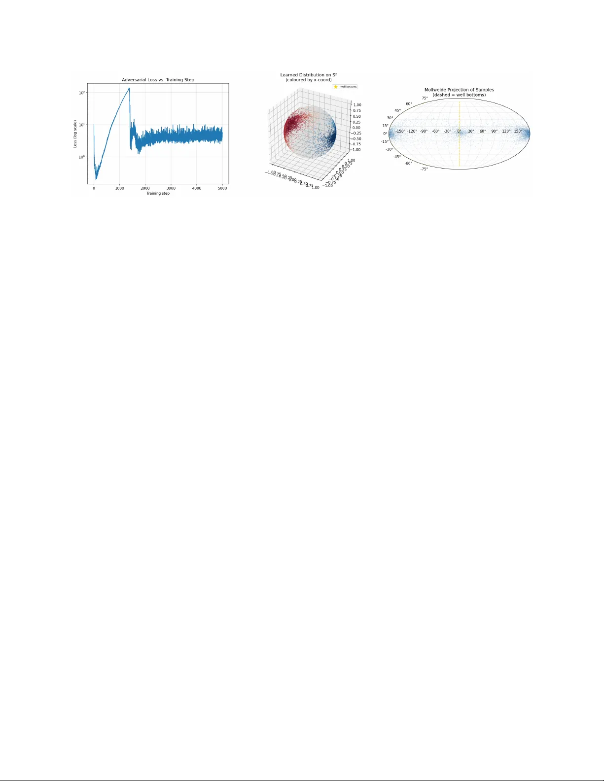
Neural Pushforw ard Samplers for the F okk er–Planc k Equation on Em b edded Riemannian Manifolds Andrew Qing He ∗ W ei Cai † Marc h 2026 Abstract In this pap er, w e extend the weak adv ersarial neural pushforward mapping metho d to the F okk er–Planck equation on compact em b edded Riemannian manifolds. The metho d represents the solution as a probability distribution via a neural pushforward map that is constrained to the manifold b y a retraction lay er, enforcing manifold mem- b ership and probability conserv ation b y construction. T raining is guided b y a weak adv ersarial ob jectiv e using ambien t plane-wa ve test functions, whose intrinsic differen- tial op erators are derived in closed form from the geometry of the embedding, yielding a fully mesh-free and c hart-free algorithm. Both steady-state and time-dep enden t for- m ulations are dev elop ed, and numerical results on a double-well problem on the t wo- sphere demonstrate the capability of the method in capturing m ultimo dal inv ariant distributions on curv ed spaces. Keyw ords: F okk er–Planck equation, Riemannian manifold, neural pushforward map, w eak adv ersarial net work, Laplace–Beltrami operator, plane-wa v e test functions, steady-state dis- tribution, sphere. MSC 2020: 65N75; 68T07; 58J65; 35Q84. Con ten ts 1 In tro duction 3 2 Setting and Notation 4 3 Steady-State W ANPF on a Manifold 4 3.1 Strong F ormulation . . . . . . . . . . . . . . . . . . . . . . . . . . . . . . . . 4 3.2 W eak F orm ulation . . . . . . . . . . . . . . . . . . . . . . . . . . . . . . . . 5 3.3 Pushforw ard Architecture and Adversarial Loss . . . . . . . . . . . . . . . . 5 ∗ Departmen t of Mathematics, Southern Metho dist Universit y , Dallas, TX 75275. andrewho@smu.edu † Departmen t of Mathematics, Southern Metho dist Universit y , Dallas, TX 75275. cai@smu.edu 1 4 Am bient Plane-W a ve T est F unctions 5 4.1 Definition . . . . . . . . . . . . . . . . . . . . . . . . . . . . . . . . . . . . . 5 4.2 Laplace–Beltrami Action on Plane W av es . . . . . . . . . . . . . . . . . . . . 6 5 Manifold-Constrained Pushforward Arc hitecture 6 5.1 Retraction-Based Generator . . . . . . . . . . . . . . . . . . . . . . . . . . . 6 5.2 Net work Sp ecification . . . . . . . . . . . . . . . . . . . . . . . . . . . . . . . 7 6 Time-Dep enden t W ANPF on a Manifold 7 6.1 W eak F orm ulation . . . . . . . . . . . . . . . . . . . . . . . . . . . . . . . . 7 6.2 Mon te Carlo Estimators . . . . . . . . . . . . . . . . . . . . . . . . . . . . . 7 6.3 Adv ersarial T raining Ob jective . . . . . . . . . . . . . . . . . . . . . . . . . . 8 7 Explicit F orm ulae for Key Manifolds 8 7.1 The Unit Sphere S n − 1 ⊂ R n . . . . . . . . . . . . . . . . . . . . . . . . . . . 8 7.2 The Flat T orus T n ⊂ R 2 n . . . . . . . . . . . . . . . . . . . . . . . . . . . . . 9 8 Numerical Exp erimen t: Double-W ell FPE on S 2 9 8.1 Problem Setup . . . . . . . . . . . . . . . . . . . . . . . . . . . . . . . . . . 9 8.2 Am bient Gradient and Drift . . . . . . . . . . . . . . . . . . . . . . . . . . . 9 8.3 Arc hitecture and T raining . . . . . . . . . . . . . . . . . . . . . . . . . . . . 9 8.4 Results . . . . . . . . . . . . . . . . . . . . . . . . . . . . . . . . . . . . . . . 10 9 Discussion 10 9.1 Adv an tages of the Manifold F orm ulation . . . . . . . . . . . . . . . . . . . . 10 9.2 Connection to Geometric Measure Theory . . . . . . . . . . . . . . . . . . . 11 9.3 Extension to Non-Isotropic Diffusion . . . . . . . . . . . . . . . . . . . . . . 11 9.4 Supplemen ting with Spherical Harmonics . . . . . . . . . . . . . . . . . . . . 12 9.5 F uture Directions . . . . . . . . . . . . . . . . . . . . . . . . . . . . . . . . . 12 10 Conclusion 13 2 1 In tro duction A wide class of stochastic differen tial equations (SDEs) arising in molecular dynamics, rob otics, directional statistics, and climate science evolv e not in flat Euclidean space but on a constrain t surface: a sphere, a torus, a Stiefel manifold, or more generally a smo oth Riemannian manifold ( M , g ) [2 – 4]. The natural companion PDE go verning the time evolu- tion of the probabilit y density is the F okker–Planc k equation (FPE) on ( M , g ), ∂ ρ ∂ t = σ 2 2 ∆ g ρ − div g ( ρ b ) , (1) where ∆ g is the Laplace–Beltrami op erator, b is a smo oth tangential drift, and σ > 0 is the diffusion co efficient. Solving (1) numerically is c hallenging for tw o indep enden t reasons. First, classical finite- difference or finite-element metho ds require an explicit triangulation of M , which b ecomes prohibitiv ely exp ensive in mo derate to high dimension. Second, ev en for simple manifolds suc h as S n − 1 with n ≥ 4, the curse of dimensionalit y prev ents grid-based metho ds from b eing practically viable. Recen t w ork has addressed these difficulties for flat-space FPEs b y represen ting the solu- tion distribution rather than a p oint wise density , through a neural pushforward map trained with a weak adversarial ob jectiv e [1]. In that approach, a generator netw ork F ϑ pushes a simple base distribution forward to appro ximate the FPE solution at any queried time, with training guided b y a three-term Monte Carlo w eak form ulation that av oids any spatial mesh. The presen t paper extends this W eak Adv ersarial Neural Pushforw ard Metho d (W ANPF) to the Riemannian setting. The extension rests on tw o structural observ ations. 1. Non-in v ertibility is an asset. The pushforward map F ϑ : R d → M need not b e in vertible, and the base dimension d need not equal dim M . This is imp ossible for normalizing-flo w or c hange-of-v ariables metho ds, and it is what allo ws W ANPF to use a higher-dimensional noise space for greater representational capacit y . 2. W eak in tegrals b ecome point wise exp ectations. After integrating b y parts, ev ery spatial op erator in the w eak form acts on the test function rather than on ρ . The Laplace–Beltrami op erator applied to an ambien t plane-w av e test function can b e computed in closed form at each sample, using only the tangential pro jection P ( x ) = I − xx ⊤ (for the sphere) and the mean-curv ature vector H ( x ). No automatic differen tiation through the intrinsic geometry is required. The result is a fully mesh-free, c hart-free, and Jacobian-free training pro cedure. The generator’s samples are constrained to M via a manifold retraction Π M (e.g., normalization to the unit sphere), and the initial condition is satisfied automatically b y the pushforward arc hitecture. Con tributions. • A complete steady-state W ANPF form ulation for the manifold FPE, including the adv ersarial min-max loss and its Monte Carlo estimator (Section 3). 3 • A time-dep endent W ANPF formulation with a three-term w eak form (Section 6), matc hing the flat-space structure of [1]. • Closed-form Laplace–Beltrami plane-wa ve form ulae for S n − 1 and T n (Sections 4 – 7). • Numerical exp erimen ts on the double-well FPE on S 2 , demonstrating that the trained generator correctly concentrates mass near the t w o Boltzmann minima (Section 8). Organization. Section 2 in tro duces the manifold FPE and fixes notation. Section 3 de- riv es the steady-state W ANPF. Section 4 derives the ambien t plane-wa ve Laplace–Beltrami form ulae. Section 5 sp ecifies the pushforward architecture. Section 6 deriv es the time- dep enden t W ANPF. Section 7 records explicit formulae for the sphere and torus. Section 8 presen ts the n umerical exp eriments. Section 9 discusses extensions. 2 Setting and Notation Throughout, ( M , g ) is a smo oth, compact, connected Riemannian manifold without b ound- ary , isometrically em b edded in R n . Compactness ensures global probabilit y conserv ation and the absence of spatial b oundary conditions. Let m = dim M ≤ n − 1. F or an y x ∈ M , let T x M ⊂ R n denote the tangen t space of M at x . W e write P ( x ) ∈ R n × n for the orthogonal pro jection onto T x M , so P ( x ) 2 = P ( x ), P ( x ) ⊤ = P ( x ), and P ( x ) v is the tangen tial comp onent of an y ambien t vector v ∈ R n . The me an-curvatur e ve ctor H ( x ) ∈ R n of the embedding is H ( x ) = tr  ∂ i P ( x )  , (2) where the trace is ov er the n co ordinate directions. F or a smooth ambien t function f : R n → R , the intrinsic gradien t and Laplace–Beltrami op erator on M are: ∇ g f ( x ) = P ( x ) ∇ f ( x ) , (3) ∆ g f ( x ) = ∇ 2 f ( x ) : P ( x ) − ∇ f ( x ) · H ( x ) , (4) where ∇ f and ∇ 2 f are the Euclidean gradien t and Hessian of the ambien t extension of f , and A : B = tr( A ⊤ B ). F or flat subspaces, H = 0 and (4) reduces to the standard Laplacian restricted to the subspace. The drift b is a smo oth tangen tial v ector field on M , and in applications derived from a p otential V : R n → R it takes the form b ( x ) = − P ( x ) ∇ V ( x ), whic h is automatically tangen tial. 3 Steady-State W ANPF on a Manifold 3.1 Strong F ormulation The steady-state FPE seeks a probability measure ρ on M satisfying: σ 2 2 ∆ g ρ − div g ( ρ b ) = 0 , Z M ρ dV ol g = 1 , ρ ≥ 0 . (5) 4 On a compact manifold without b oundary the F redholm alternativ e guarantees the existence and, under mild irreducibilit y conditions on b , the uniqueness of an in v ariant measure. When b = −∇ g V for a p oten tial V , the unique inv ariant measure is the Gibbs distribution ρ ∞ ∝ e − 2 V /σ 2 . 3.2 W eak F orm ulation Multiplying (5) by a test function f ∈ C ∞ ( M ), integrating ov er M against dV ol g , and in tegrating by parts (b oundary terms v anish by compactness) giv es: Z M ρ ( x ) L ss f ( x ) dV ol g = 0 , (6) where the b ackwar d Kolmo gor ov op er ator for the steady-state problem is: L ss f := σ 2 2 ∆ g f + ⟨ b , ∇ g f ⟩ g . (7) Equation (6) is an exp ectation condition: E x ∼ ρ [ L ss f ( x )] = 0 ∀ admissible f . (8) 3.3 Pushforw ard Arc hitecture and Adv ersarial Loss F or the steady-state problem the pushforward map has no temp oral argumen t: F ϑ : R d → M , F ϑ ( r ) = Π M  ˜ F ϑ ( r )  , (9) where ˜ F ϑ : R d → R n is an unconstrained MLP and Π M is the manifold retraction (Section 5). Giv en M s samples r ( m ) ∼ P base and K adversarial test functions { f ( k ) } , the empirical esti- mator is ˆ E ( k ) = 1 M s M s X m =1 L ss f ( k )  F ϑ ( r ( m ) )  . (10) The adversarial training ob jective is the min-max problem: min ϑ max { η ( k ) } 1 K K X k =1  ˆ E ( k )  2 , (11) where η ( k ) = { w ( k ) , b ( k ) } are the test-function parameters defined in Section 4. 4 Am bien t Plane-W a v e T est F unctions 4.1 Definition F ollowing the flat-space W ANPF [1], the test functions are ambien t plane wa v es: f ( k ) ( x ) = sin  w ( k ) · x + b ( k )  , k = 1 , . . . , K , (12) with learnable parameters w ( k ) ∈ R n and b ( k ) ∈ R . F or the time-dep endent case an additional temp oral phase κ ( k ) t is included (Section 6). 5 4.2 Laplace–Beltrami Action on Plane W a v es Setting ϕ ( k ) := w ( k ) · x + b ( k ) , the am bien t Euclidean deriv ativ es are ∇ f ( k ) = cos( ϕ ( k ) ) w ( k ) and ∇ 2 f ( k ) = − sin( ϕ ( k ) ) w ( k ) ( w ( k ) ) ⊤ . Substituting in to (4) gives the key form ula: ∆ g f ( k )   M = − sin( ϕ ( k ) ) ( w ( k ) ) ⊤ P ( x ) w ( k ) − cos( ϕ ( k ) ) H ( x ) · w ( k ) . (13) The first term in volv es the pr oje cte d squar e d fr e quency | w | 2 P := w ⊤ P ( x ) w , and the second is a curv ature correction prop ortional to H ( x ) · w . Both are computable without automatic differen tiation once P ( x ) and H ( x ) are known for the sp ecific manifold. Remark 4.1 (Flat-space reco v ery) . F or M = R n one has P = I n and H = 0 , so ∆ g f ( k ) = −| w ( k ) | 2 sin ϕ ( k ) , r e c overing the standar d W ANPF formula [1]. Remark 4.2 (Non-eigenfunction c haracter) . Unlike in flat sp ac e, plane waves ar e not eigen- functions of ∆ g on a curve d manifold: the curvatur e c orr e ction intr o duc es a cos ϕ term that mixes phases. Nevertheless, as adversarial ly optimize d test pr ob es, they r emain effe ctive. Using (13) and the tangential drift formula ⟨ b ( x ) , ∇ g f ( k ) ( x ) ⟩ g = cos( ϕ ( k ) ) ⟨ P ( x ) b ( x ) , w ( k ) ⟩ , the backw ard Kolmogoro v op erator on a steady-state plane w a ve ev aluates to: L ss f ( k ) ( x ) = − σ 2 2 sin( ϕ ( k ) ) ( w ( k ) ) ⊤ P ( x ) w ( k ) − σ 2 2 cos( ϕ ( k ) ) H ( x ) · w ( k ) + cos( ϕ ( k ) ) ⟨ P ( x ) b ( x ) , w ( k ) ⟩ . (14) All three terms are closed-form at each sample on M . 5 Manifold-Constrained Pushforw ard Arc hitecture 5.1 Retraction-Based Generator The pushforward map must satisfy F ϑ ( t, x 0 , r ) ∈ M for all arguments. W e achiev e this by comp osing an unconstrained residual net w ork ˜ F ϑ : R 1+ n + d → R n with a manifold retraction Π M : F ϑ ( t, x 0 , r ) = Π M  x 0 + √ t ˜ F ϑ ( t, x 0 , r )  . (15) Here x 0 ∼ ρ 0 is an initial sample on M and r ∼ P base is a d -dimensional noise vector. The √ t prefactor ensures that F ϑ (0 , x 0 , r ) = Π M ( x 0 ) = x 0 since x 0 ∈ M already , so the initial condition ρ (0 , · ) = ρ 0 is satisfied automatically . F or commonly encoun tered manifolds the retraction Π M has an analytical form: • Sphere S n − 1 : Π M ( v ) = v / ∥ v ∥ . • Stiefel manifold St( n, k ): p olar retraction Π( V ) = V ( V ⊤ V ) − 1 / 2 . • Flat torus T n : comp onent wise wrapping Π( v ) =  cos v i , sin v i  n i =1 . 6 Remark 5.1 (Parametrization alternativ e) . When M admits a glob al chart ψ : R m → M (e.g., ster e o gr aphic pr oje ction for S n − 1 , or the exp onential map for Lie gr oups), one c an inste ad define F ϑ := ψ ( ξ ϑ ) wher e ξ ϑ is a network in the p ar ameter sp ac e R m . This avoids the pr oje ction step but intr o duc es chart singularities for most manifolds of inter est; the r etr action appr o ach (15) is ther efor e pr eferr e d. 5.2 Net w ork Sp ecification F or the sphere exp erimen ts in Section 8 we use a ste ady-state generator (no t or x 0 argumen t): F ϑ ( r ) = ˜ F ϑ ( r ) ∥ ˜ F ϑ ( r ) ∥ , ˜ F ϑ : R d MLP − − − → R 3 , (16) with tanh activ ations throughout. The netw ork dimensions and training h yp erparameters are listed in T able 1. 6 Time-Dep enden t W ANPF on a Manifold 6.1 W eak F orm ulation Let f ∈ C ∞ ([0 , T ] × M ) b e a smo oth test function. Multiplying the time-dep endent FPE (1) b y f , in tegrating ov er M × [0 , T ], and in tegrating by parts in both time and space (b oundary terms v anish b y compactness) giv es: Z M f ( T , x ) ρ ( T , x ) dV ol g − Z M f (0 , x ) ρ 0 ( x ) dV ol g − Z T 0 Z M ρ ( t, x )  ∂ t f + σ 2 2 ∆ g f + b ( f )  dV ol g dt = 0 . (17) Since the pushed-forw ard samples x ( t ) = F ϑ ( t, x 0 , r ) are distributed according to ρ ( t, · ) when ϑ is correct, the identit y (17) b ecomes three Monte Carlo estimable terms: ˆ E ( k ) T − ˆ E ( k ) 0 − ˆ E ( k ) = 0 , (18) with the time-dep endent plane-w a ve test functions: f ( k ) ( t, x ) = sin  w ( k ) · x + κ ( k ) t + b ( k )  , (19) where κ ( k ) ∈ R is a learnable temp oral frequency . 6.2 Mon te Carlo Estimators Let ϕ ( k ) := w ( k ) · x + κ ( k ) t + b ( k ) . The three estimators in (18) are: T erminal term. Dra w M T samples x ( m ) 0 ,T ∼ ρ 0 and r ( m ) T ∼ P base : ˆ E ( k ) T = 1 M T M T X m =1 f ( k )  T , F ϑ  T , x ( m ) 0 ,T , r ( m ) T   . (20) 7 Initial term. Draw M 0 samples x ( m ) 0 ∼ ρ 0 directly: ˆ E ( k ) 0 = 1 M 0 M 0 X m =1 f ( k )  0 , x ( m ) 0  . (21) In terior term. Draw M triples t ( m ) ∼ U (0 , T ), x ( m ) 0 ∼ ρ 0 , r ( m ) ∼ P base , and set x ( m ) = F ϑ ( t ( m ) , x ( m ) 0 , r ( m ) ): ˆ E ( k ) = T M M X m =1 h κ ( k ) cos( ϕ ( k ) ) + σ 2 2 ∆ g f ( k ) + cos( ϕ ( k ) ) ⟨ P ( x ) b ( x ) , w ( k ) ⟩ i  t ( m ) , x ( m )  , (22) where ∆ g f ( k ) is ev aluated via (13). 6.3 Adv ersarial T raining Ob j ectiv e The total loss aggregates the squared residuals o ver all K test functions: L total [ ϑ , { η ( k ) } ] = 1 K K X k =1  ˆ E ( k ) T − ˆ E ( k ) 0 − ˆ E ( k )  2 , (23) with η ( k ) = { w ( k ) , κ ( k ) , b ( k ) } . T raining follo ws the min-max scheme: min ϑ max { η ( k ) } L total . (24) The generator (minimiser) and test-function netw ork (maximiser) are updated with separate Adam optimisers, with gradien t ascent for the adv ersary and gradien t descen t (with gradien t clipping) for the generator. 7 Explicit F orm ulae for Key Manifolds W e record the pro jection matrix P ( x ), the mean-curv ature vector H ( x ), and the result- ing Laplace–Beltrami form ula (13) for the tw o manifolds most frequen tly encoun tered in applications. 7.1 The Unit Sphere S n − 1 ⊂ R n F or x ∈ S n − 1 (i.e. ∥ x ∥ = 1), the tangen tial pro jection and mean-curv ature vector are: P ( x ) = I n − xx ⊤ , H ( x ) = − ( n − 1) x. (25) Substituting into (13) giv es: ∆ g f ( k )   S n − 1 = − sin( ϕ ( k ) )  | w ( k ) | 2 − ( x · w ( k ) ) 2  + ( n − 1) cos( ϕ ( k ) ) ( x · w ( k ) ) . (26) F or S 2 ⊂ R 3 (i.e. n = 3) the constan t factor is n − 1 = 2. 8 7.2 The Flat T orus T n ⊂ R 2 n Em b ed the n -torus as M = { (cos θ i , sin θ i ) n i =1 } ⊂ R 2 n . The tangen t space is spanned b y the n v ectors e i = (0 , . . . , − sin θ i , cos θ i , . . . , 0) ⊤ , and the mean-curv ature v ector v anishes b ecause eac h factor is a unit circle: H ( x ) = 0. W riting w = ( w c 1 , w s 1 , . . . , w c n , w s n ) ⊤ ∈ R 2 n , the pro jected squared frequency is: w ⊤ P ( x ) w = n X i =1  − w c i sin θ i + w s i cos θ i  2 , (27) and therefore ∆ g f ( k ) = − sin( ϕ ( k ) ) w ⊤ P ( x ) w , with no curv ature correction. 8 Numerical Exp erimen t: Double-W ell FPE on S 2 8.1 Problem Setup W e consider the steady-state F okk er–Planck equation (5) on the unit sphere S 2 ⊂ R 3 with diffusion co efficient σ = 0 . 5 and p oten tial-deriv ed drift b ( x ) = − P ( x ) ∇ V ( x ). The p otential is a double-well function on R 3 restricted to S 2 : V ( x, y , z ) = α ( x 2 − 1) 2 + β z 2 , α = 4 . 0 , β = 2 . 0 . (28) The t w o w ells of V are lo cated at ( ± 1 , 0 , 0) on S 2 , where V = 0. The β z 2 term confines mass to the equatorial band and prev en ts the distribution from spreading tow ard the p oles. Figure 1 shows the p oten tial V in longitude–latitude co ordinates. The Gibbs in v ariant measure is ρ ∞ ( x ) ∝ e − 2 V ( x ) /σ 2 , which concentrates sharply near ( ± 1 , 0 , 0) for the c hosen parameters. 8.2 Am bien t Gradien t and Drift The Euclidean gradient of V is: ∇ V ( x, y , z ) =  4 α ( x 2 − 1) x, 0 , 2 β z  ⊤ . (29) The manifold drift b ( x ) = − P ( x ) ∇ V ( x ) is then obtained b y pro jecting −∇ V on to the tangen t plane of S 2 at x , using P ( x ) = I 3 − xx ⊤ . 8.3 Arc hitecture and T raining The generator is a tw o-lay er MLP with width 32 and tanh activ ations, mapping a d = 3- dimensional standard Gaussian base distribution r ∼ N (0 , I 3 ) to S 2 via normalization: F ϑ ( r ) = ˜ F ϑ ( r ) ∥ ˜ F ϑ ( r ) ∥ . (30) The adv ersarial test functions are K = 200 am bient plane wa v es (12) with parameters initialized as w ( k ) ∼ N (0 , 4 I 3 ) and b ( k ) ∼ N (0 , 0 . 25). The L ss f ( k ) ( x ) ev aluator uses the 9 T able 1: Hyp erparameters for the S 2 double-w ell exp eriment. P arameter Sym b ol V alue Diffusion co efficient σ 0 . 5 Base dimension d 3 Generator hidden width — 32 Generator depth — 2 lay ers Num b er of test functions K 200 Mon te Carlo batc h size M s 200 T raining steps N 5 , 000 Generator learning rate η ϑ 10 − 3 (cosine annealing) Adv ersary learning rate η η 5 × 10 − 3 P otential parameters α, β 4 . 0 , 2 . 0 closed-form form ula (14) sp ecialized to S 2 via (26), with no automatic differen tiation through the geometry . T raining h yp erparameters are summarized in T able 1. The training lo op alternates one adv ersary gradien t-ascent step (maximizing the loss o ver { η ( k ) } ) with one generator gradien t-descent step (minimizing the loss ov er ϑ ), with gradien t clipping of norm 1 . 0 applied to the generator. A cosine annealing schedule is applied to the generator learning rate from 10 − 3 do wn to 10 − 5 o ver the 5 , 000 steps. 8.4 Results Figure 1 shows the double-w ell p oten tial V on S 2 in a longitude–latitude (Plate Carr´ ee) pro- jection alongside the histogram of learned sample densit y pro duced b y the trained generator. Figure 2 shows additional diagnostics: the adversarial training loss on a log scale, the pushed-forw ard samples on the sphere coloured b y the x -coordinate, and a Mollweide pro- jection of the samples. The key qualitativ e observ ations are as follows. The learned distribution concen trates mass near b oth well b ottoms at ( ± 1 , 0 , 0) and is strongly suppressed near the p oles, as exp ected from the β z 2 confinemen t term in V . The approximate symmetry betw een the t w o w ells is preserv ed, reflecting the x → − x symmetry of V . The training loss conv erges to a stationary level after appro ximately 2 , 000 steps, with subsequent fluctuations characteristic of the min-max adv ersarial dynamics. 9 Discussion 9.1 Adv an tages of the Manifold F ormulation The manifold W ANPF inherits all structural adv antages of the flat-space metho d [1]: samples are generated rather than a p oint wise densit y , so probability conserv ation is exact; the w eak form ulation requires no mesh, no chart atlas, and no Jacobian determinant; and the metho d handles multimodal distributions without any explicit mixture structure. 10 Figure 1: Left: the double-w ell p oten tial V ( x, y , z ) = α ( x 2 − 1) 2 + β z 2 on S 2 , sho wn in longitude–latitude pro jection. The tw o p otential minima ( V = 0) are lo cated at longitude 0 ◦ and ± 180 ◦ on the equator, corresp onding to ( ± 1 , 0 , 0). Righ t: density histogram of 8 , 000 samples generated b y the trained neural pushforw ard map in the same co ordinate system. Mass concentrates near b oth well b ottoms and is absent near the p oles, consisten t with the Gibbs distribution ρ ∞ ∝ e − 2 V /σ 2 for σ = 0 . 5. The manifold extension adds t wo further b enefits. First, the retraction arc hitecture F ϑ = Π M ◦ ˜ F ϑ k eeps all samples on M at no additional training cost beyond a single pro jection p er forw ard pass. Second, the closed-form Laplace–Beltrami formula (13) b ypasses all automatic differen tiation through the geometry of M , making the p er-step cost indep endent of the n umber of la y ers in the intrinsic differential op erators. 9.2 Connection to Geometric Measure Theory The use of am bient test functions is consisten t with the theory of v arifolds, where the k ey iden tity Z M ρ ∆ g f dV ol g = Z M ρ  ∇ 2 f : P − ∇ f · H  dV ol g (31) expresses the Laplace–Beltrami action en tirely through am bient quan tities ev aluated on sam- ples in R n [5]. W ANPF exploits precisely this iden tity . 9.3 Extension to Non-Isotropic Diffusion The deriv ation extends directly to the general FPE with a diffusion tensor a (a positive- definite (2 , 0)-tensor on M ). The backw ard Kolmogorov op erator b ecomes L f = 1 2 div g ( a (d f ))+ b ( f ), and in ambien t co ordinates: L f = 1 2 ∇ 2 f : P AP ⊤ − 1 2 ( AP ⊤ ∇ f ) · H + ⟨ P b , P ∇ f ⟩ , (32) 11 Figure 2: T raining and sampling diagnostics for the S 2 double-w ell exp erimen t. Left: adv er- sarial loss v ersus training step (log scale). The loss rises during early generator exploration and then decreases as training conv erges to a stationary min-max p oint near step 2 , 000. Cen- ter: 8 , 000 generated samples on S 2 , coloured by their x -co ordinate v alue (red near x = +1, blue near x = − 1); gold stars mark the t wo well b ottoms ( ± 1 , 0 , 0). The generator correctly concen trates mass around b oth minima symmetrically . Right: Mollw eide equal-area pro- jection of the same samples; dashed gold lines indicate the longitudes of the w ell b ottoms. Samples cluster near 0 ◦ and ± 180 ◦ longitude, confirming tw o-w ell capture, with near-uniform spreading in longitude about eac h minimum and strong equatorial confinement consisten t with the β z 2 term. where A ∈ R n × n is any ambien t extension of a . F or the isotropic case a = σ 2 g − 1 , P AP ⊤ = σ 2 P and (32) reduces to (14). 9.4 Supplemen ting with Spherical Harmonics As noted in Remark 4.2, ambien t plane w a ves are not eigenfunctions of ∆ g on a curv ed manifold. F or S n − 1 , one could supplemen t the plane-w a ve test-function class with spherical harmonics Y m ℓ , which ar e eigenfunctions with eigenv alue − ℓ ( ℓ + n − 2). In the W ANPF framew ork this amounts to adding additional test functions whose op erator ev aluations are analytically known; the min-max training structure is unc hanged. W e lea ve a systematic comparison to future w ork. 9.5 F uture Directions Sev eral extensions are natural. The time-dependent formulation (Section 6) is directly ap- plicable to the heat equation on S n − 1 or on a Lie group suc h as SO(3); the only c hange is the sp ecification of P ( x ) and H ( x ) for the new manifold. F or the fractional F okker–Planc k equation on a manifold, one w ould need to replace the Laplace–Beltrami op erator with the sp ectral fractional Laplacian ( − ∆ g ) α/ 2 , whose plane-wa v e action on curved manifolds is no longer as clean but could b e approximated via Mon te Carlo integration ov er manifold heat k ernels. Higher-dimensional manifolds (e.g., S n − 1 with n ≥ 10) are a natural stress test for the mesh-free approach. 12 10 Conclusion W e hav e extended the W eak Adv ersarial Neural Pushforw ard Metho d to the F okker–Planc k equation on compact em b edded Riemannian manifolds. The extension rests on three pillars: (i) a retraction-based pushforward arc hitecture that k eeps samples on M by construction; (ii) am bient plane-w av e test functions whose Laplace–Beltrami op erators are computable in closed form via the tangential pro jection P ( x ) and mean-curv ature v ector H ( x ); and (iii) a min-max adv ersarial loss whose Mon te Carlo estimator requires only p oint wise ev aluations at samples on M , with no mesh, no c hart, and no Jacobian computation. The resulting algorithm for the steady-state case is summarized in Algorithm 1. Numer- ical exp eriments on the double-w ell FPE on S 2 confirm that the trained generator correctly concen trates mass near b oth p otential minima, consistent with the Gibbs inv ariant measure. Algorithm 1 Steady-State Manifold W ANPF Require: manifold M with retraction Π M , P ( · ), H ( · ); drift b ; diffusion σ ; learning rates η ϑ , η η ; batch size M s ; steps N . 1: Initialize generator F ϑ and test-function parameters { η ( k ) } K k =1 . 2: for step = 1 , . . . , N do 3: Adv ersary step: sample { r ( m ) } , compute x ( m ) = F ϑ ( r ( m ) ) ∈ M , ev aluate ˆ E ( k ) via (10) and (14), up date η ( k ) += η η ∇ η L (gradient ascent). 4: Generator step: same forward pass, up date ϑ − = η ϑ ∇ ϑ L (gradient descent). 5: end for Ensure: generator F ϑ appro ximating the in v ariant measure ρ ∞ . The framework is directly applicable to an y manifold for which P ( x ) and H ( x ) can b e computed analytically or n umerically , and it scales to dimensions inaccessible b y mesh-based solv ers. References [1] A. Q. He and W. Cai, Neural Pushforw ard Samplers for T ransien t Distributions from F okker–Planc k Equations with W eak Adv ersarial T raining, , 2025. [2] E. P . Hsu, Sto chastic A nalysis on Manifolds , Graduate Studies in Mathematics, vol. 38. American Mathematical So ciety , Pro vidence, RI, 2002. [3] M. Girolami and B. Calderhead, Riemann manifold Langevin and Hamiltonian Monte Carlo metho ds, Journal of the R oyal Statistic al So ciety: Series B , 73(2):123–214, 2011. [4] N. Lei, K. Su, L. Cui, S.-T. Y au, and D. X. Gu, A geometric view of optimal trans- p ortation and generative mo del, Computer Aide d Ge ometric Design , 68:1–21, 2019. [5] L. Simon, L e ctur es on Ge ometric Me asur e The ory , Pro ceedings of the Centre for Mathematical Analysis, vol. 3. Australian National Univ ersit y , Can b erra, 1983. 13 [6] Y. Zang, G. Bao, X. Y e, and H. Zhou, W eak adversarial net works for high-dimensional partial differential equations, Journal of Computational Physics , 411:109409, 2020. [7] M. Raissi, P . Perdik aris, and G. E. Karniadakis, Physics-informed neural netw orks: A deep learning framework for solving forward and inv erse problems inv olving nonlinear partial differential equations, Journal of Computational Physics , 378:686–707, 2019. [8] E. W einan and B. Y u, The deep Ritz metho d: a deep learning-based n umerical algorithm for solving v ariational problems, Communic ations in Mathematics and Statistics , 6(1):1– 12, 2018. 14