Deep learning and the rate of approximation by flows

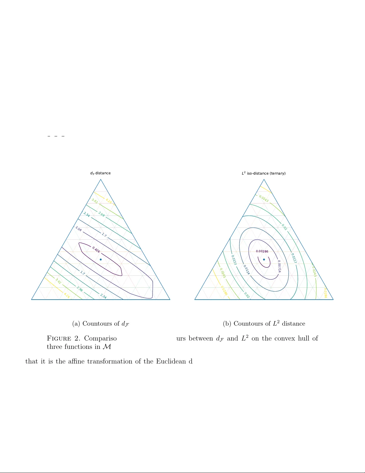
DEEP LEARNING AND THE RA TE OF APPR O XIMA TION BY FLO WS JINGPU CHENG 1 , QIANXIA O LI 2 , TING LIN 3 , AND ZUO WEI SHEN 4 Abstract. W e in vestigate the dep endence of the appro ximation capacity of deep residual netw orks on its depth in a con tinuous dynamical systems setting. This can b e formulated as the general problem of quan tifying the minimal time-horizon required to appro ximate a diﬀeomorphism b y ﬂo ws driven by a given family F of v ector ﬁelds. W e sho w that this minimal time can be iden tiﬁed as a geodesic distance on a sub- Finsler manifold of diﬀeomorphisms, where the lo cal geometry is characterised b y a v ariational principle in volving F . This connects the learning eﬃciency of target relationships to their compatibility with the learning arc hitectural choice. F urther, the results suggest that the key approximation mec hanism in deep learning, namely the approximation of functions by comp osition or dynamics, diﬀers in a fundamental w ay from linear appro ximation theory , where linear spaces and norm-based rate estimates are replaced b y manifolds and geo desic distances. Contents 1. In tro duction 1 2. Problem form ulation and main results 4 2.1. Notations 4 2.2. F ormulation and main results 4 2.3. Implications for appro ximation theory and comp ositional mo dels 7 3. The rate of appro ximation b y ﬂo ws: one dimensional ReLU netw orks 9 3.1. Pro ofs of the results for 1D ReLU control family 12 4. The rate of appro ximation b y ﬂo ws: the general case 22 4.1. Preliminaries on Banac h sub-Finsler geometry 22 4.2. General c haracterization of appro ximation complexit y via Finsler geometry 27 4.3. In terp olation distance, v ariational formula and asymptotic prop erties 32 5. Applications 36 5.1. 1D ReLU revisited 36 5.2. Other applications 39 Computations for the la y er-normalization example 45 References 50 1. Intr oduction Deep residual netw orks (ResNets) form the bac kb one of mo dern deep learning architectures, ranging from conv olution net works for image pro cessing [ 20 ] to transformers p o wering large language mo dels 1 Dep ar tment of Ma thema tics, Na tional University of Singapore, 117543, Singapore 2 Dep ar tment of Ma thema tics and Institute for Functional Intelligent Ma terials, Na tional Univer- sity of Singapore, 117543, Singapore 3 School of Ma thema tical Sciences, Peking University, 100871, China 4 Dep ar tment of Ma thema tics, Na tional University of Singapore, 117543, Singapore E-mail addr esses : chengjingpu@u.nus.edu, qianxiao@nus.edu.sg, lintingsms@pku.edu.cn, matzuows@nus.edu.sg . Date : Marc h 19, 2026. 1 2 DEEP LEARNING AND THE RA TE OF APPRO XIMA TION BY FLOWS [ 48 ]. A t the same time, their success also p ose interesting new mathematical questions. A deep residual net w ork is built from rep eated comp ositions of transformations (1.1) x ( n + 1) = x ( n ) + f n ( x ( n )) , f n ∈ F , n = 0 , 1 , 2 , . . . , N − 1 , where N is the depth of the netw ork, x ( n ) ∈ R d is the hidden state of the net w ork at lay er n and f n : R d → R d is the trainable non-linear transformation applied at each lay er, with F b eing the set of p ossible transformations that is determined b y the arc hitectural c hoice. F or example, in fully connected ResNets, F is the set of all functions that can b e represented b y a single-la yer feedforw ard net w ork [ 47 , 46 , 18 ], whereas for transformers, F is the set of tok en-wise netw orks composed with self-atten tion maps [ 48 , 13 , 15 ]. With this comp ositional structure, one can build complex transformations x (0) 7→ x ( N ) b y increasing the num ber of lay ers N , and this is the main wa y of improving mo del learning capacity in mo dern artiﬁcial in telligence applications. These fall into the following tw o complementary formulations. (i) Appro ximation of functions in sup ervised learning. In standard sup ervised learning tasks, w e consider a set of inputs X ⊂ R d and a set of outputs Y ⊂ R m . The goal of learning is to approximate an unkno wn target function F : X → Y that maps inputs to outputs. F or example, X can b e the set of natural images represented by pixel in tensities, and Y is the corresp onding classiﬁcation of the image in to types, such as cats, birds, cars, etc. F wou ld then b e the function that classify a given image in to its t yp e, realising an image recognition to ol. Residual net w orks tackles this appro ximation problem by considering the comp osition (1.2) ˜ F := β ◦ ϕ N ◦ α, where x (0) 7→ ϕ N ( x (0)) = x ( N ) is the map deﬁned b y the N -la y er residual dynamics in ( 1.1 ), and α : X → R d and β : R d → Y are simple maps (e.g., β can b e aﬃne functions for regression problems and indicator functions of a half-space for binary classiﬁcation problems). The function ˜ F is then used to approximate the target F , with its approximation capacity imparted b y the large num ber of building blo c ks in ϕ N . (ii) Approximations of distributions in generative mo delling. Another highly relev ant applica- tion relying on a similar dynamical approximation sc heme is generative mo delling [ 31 , 21 , 40 ], where the goal is to learn a mo del that can generate samples (e.g. images, text, crystal structure, etc.) from a target data distribution. In this case, a predominant approach is to mo del a transp ort map that pushes forw ard a simple reference distribution µ 0 (e.g., a Gaussian) to a complicated target data distribution µ 1 . More concretely , w e aim to ﬁnd a map ϕ such that (1.3) ϕ # µ 0 ≈ µ 1 . In practice, such transp ort maps are often mo delled as the ﬂow map of an ODE realized by the deep residual structure [ 21 , 40 , 42 , 31 ] (serving as a discrete approximation) in ( 1.1 ). In b oth scenarios discussed ab ov e, one requires the comp ositions of residual lay ers to appro ximate a complicated transformation on X . A primary mathematical question that arises is: how do es such comp ositional structures build complexit y , and ho w is it diﬀeren t from c lassical methods — suc h as ﬁnite elemen ts, splines, and wa v elets — whic h typically rely on linear combinations of simpler functions? A con v enient wa y to study this is the dynamic al systems approac h, whic h idealises the compositions in ( 1.1 ) as a con tin uous dynamics (1.4) ˙ x ( t ) = f t ( x ( t )) , f t ∈ F , t ∈ [0 , T ] . This connects the problem of expressivity of deep ResNets to the study of the approximation or control- labilit y prop erties of ﬂows of diﬀeren tial equations, and this approac h has yielded a n umber of insights in deep learning [ 26 , 45 , 2 , 33 , 8 ], Most notably , it was shown under fairly w eak assumptions on F that the family of ﬂo w maps of ( 1.4 ) is dense in appropriate spaces of maps from R d to itself [ 26 , 8 ]. This DEEP LEARNING AND THE RA TE OF APPRO XIMA TION BY FLOWS 3 implies in particular that as long as ResNets are suﬃciently deep, they can b e used to solve arbitrary tasks, suc h as image recognition, language mo delling and reinforcement learning. Ho w ever, the follow-up (and p erhaps the more imp ortan t) question remains: what maps from R d to itself are more easily appro ximated by a relatively shallow net w ork as opp osed to a very deep one? This connects to the imp ortan t practical problem of why and when one should use deep learning o v er other appro ximation sc hemes. A precise answ er to this question is th us important in both theory and practice. There are familiar analogues in classical approximation theory for whic h the corresp onding issues are well-understoo d. F or example, while W eierstrass [ 14 ] sho wed that p olynomials are dense in the space of contin uous functions on the unit interv al, it do es not tell us which contin uous functions can b e appro ximated well with a low p olynomial order. The classical theorem due to Jac kson [ 14 ] provides an answ er to this question, where it is sho wn that (1.5) inf p ∈P n ∥ F ( x ) − p ( x ) ∥ C ([0 , 1]) ≲ ∥ F ( α ) ∥ C ([0 , 1]) n − α , F ∈ C α ([0 , 1]) , where P n is the set of p olynomials with degree up to and including n , α is a p ositiv e integer, and F ( α ) is the order α deriv ativ e of F , whic h we assume to b e α -times contin uously diﬀerentiable. Jackson’s theorem iden tiﬁes a prop er subset of contin uous functions ( C ( α ) ) as target function spaces, on which we can establish a r ate of appr oximation . In particular, w e see that the smoother the target is, the faster the rate of appro ximation 1 . Under the same smoothness condition, a function with a smaller ∥ · ∥ C ([0 , 1]) admits a low er approximation error. This is a measure of the c omplexity of a target function under p olynomial appro ximation. This result has immediate practical consequences: w e no w understand that it is precisely the contin uously diﬀerentiable functions that admit eﬀectiv e approximations b y p olynomials, and the complexit y is go verned by the size of its deriv atives – the smaller the b etter. The purp ose of this pap er is to study the parallel problem for appro ximation b y ﬂows, as in eq. ( 1.4 ). In our setting, the cost is not the n um b er of terms in a linear com bination of monomials (p olynomial degree) but the depth of the residual arc hitecture, idealised as the time horizon T in eq. ( 1.4 ). W e ask: for whic h target maps can the ﬂow appro ximate arbitrarily w ell within a ﬁnite time T , and ho w do es the minimal suc h T dep end on the target and our c hoice of architecture F ? W e view this minimal time as a notion of complexity of the target. This diﬀers subtly from the classical Jackson-st yle question, which ﬁxes a budget (e.g., degree n ) and b ounds the approximation error as a function of that budget. Here w e in v ert the p ersp ectiv e: for a prescrib ed accuracy (arbitrarily small), we seek the minimal budget T that mak es the approximation p ossible. A simple linear analogy illustrates this distinction. Consider a Hilb ert space H with an orthonormal basis { e i } i ≥ 1 . If one ﬁxes a linear budget S (say , an  1 or  2 constrain t on co eﬃcien ts), the set of functions that can b e approximated arbitrarily w ell under that budget is just the corresp onding ball in H – a trivial c haracterisation. By contrast, in the comp ositional/ﬂo w setting the hypothesis class is closed under comp osition, not addition, and the resulting minimal-budget c haracterisation is non-trivial. This is precisely the ob ject we will study . The problem of minimal time of ﬂows for appro ximation has b een studied in sp eciﬁc settings in previous w orks. F or instance, in [ 33 ], the authors studied the appro ximation using con tin uous-time ResNets with ReLU type activ ations. They pro vided an upp er b ound on the time to ac hiev e a certain accuracy for general L 2 functions. In [ 26 ], the authors provide a quantitativ e estimate on the minimal reachable time in 1D case for ReLU activ ations. In [ 17 ], the estimation of time for interpolating a set of measures using ﬂow-based mo dels with self-attention lay ers is studied. These w orks mainly fo cus on sp eciﬁc architectures and are based on constructive approaches. In con trast, our purp ose is to develop a general framework for studying the minimal time problem for general ﬂow-based mo dels using a geometric viewp oin t. W e no w giv e a informal preview of the main results and insigh ts. First, we show that the righ t space of maps on which we can quantify ﬂow appro ximation should b e a metric space resp ecting the comp ositional structure of the problem. That is, instead of discussing the complexity of approximating 1 A conv erse due to Bernstein [ 14 ] shows that an approximation error deca y rate of n α + δ ( δ > 0) implies F ∈ C ( α ) , meaning that only smo oth functions can b e eﬃciently approximated. 4 DEEP LEARNING AND THE RA TE OF APPRO XIMA TION BY FLOWS one map, w e should instead study the complexity of connecting two maps b y a ﬂow. The appro ximation complexit y will then b e identiﬁed with the metric on this space. Next, this global picture is then supplemen ted by a lo cal one, where w e show that the metric is realised as the geo desic distance on this metric space viewed as a sub-Finsler manifold. Most imp ortantly , the lo cal lengths (Finsler norms) are c haracterised in a v ariational form in v olving the family of v ector ﬁelds F . T ogether, this giv es a concrete picture of the quantitativ e asp ects of ﬂo w (ResNet) appro ximation: the complexity of connecting t wo giv en maps b y a con tin uous deep ResNet is a distance on a manifold of target maps, where the lo cal geometry is generated by the expressiv eness of eac h shallo w lay er architecture of the deep net w ork. This framew ork addresses the basic question of quan titative measures of complexit y for approximation via deep arc hitectures, and holds for in general dimensions and arc hitecture choices. In section 5 we giv e some examples of this approach for problems where the precise manifold can b e identiﬁed and its asso ciated geo desic distances can b e computed or estimated. 2. Pr oblem formula tion and main resul ts In this section, we summarize our main results on the geometric framework for the complexit y class of ﬂo w appro ximation. W e b egin by in tro ducing the notations and the precise form ulation of the problem, follo w ed by the statement and explanation of the main results. 2.1. Notations. In the following, for a ﬁnite-dimensional manifold M , a vector ﬁeld f ∈ V ec( M ) and time t ≥ 0, w e denotes its ﬂo w map ϕ t f as: (2.1) ϕ t f : x (0) → x ( t ) , ˙ x ( t ) = f ( x ( t )) . W e adopt the following conv en tion whenever p ossible: (1) W e use f , g to denote the v ector ﬁelds and ϕ t f as the ﬂo w map of f at time horizon t . (2) W e use ψ , ξ , to denote the target mappings from a manifold M to itself. (3) W e use u, v to denote tangent vectors. Let X b e a vector space. W e write X ∥·∥ as the closure of X under the norm ∥ · ∥ . Moreo v er, if there is a natural linear inclusion X ∥·∥  → Y to some classical space Y , w e will iden tify b oth X and X ∥·∥ as their image in Y under this inclusion. F or u : M → R k , w e write u ∈ W 1 , ∞ ( M ) if u ∈ L ∞ ( M ) and its (weak) deriv ative satisﬁes ∇ u ∈ L ∞ ( M ). W e equip it with the norm (2.2) ∥ u ∥ W 1 , ∞ ( M ) := ∥ u ∥ L ∞ ( M ) + ∥∇ u ∥ L ∞ ( M ) . F or a vector ﬁeld f ∈ V ec( M ), w e interpret f ∈ W 1 , ∞ ( M ) comp onent-wise in lo cal charts (equiv alen tly , via any ﬁxed smo oth atlas on compact M ). W e write Diﬀ W 1 , ∞ ( M ) for the group of homeomorphisms ψ : M → M whose co ordinate represen tations b elong to W 1 , ∞ , i.e. (2.3) ψ , ψ − 1 ∈ W 1 , ∞ ( M ) . 2.2. F orm ulation and main results. Let M ⊂ R d b e a smo oth compact manifold (p ossibly with b oundary). Consider the follo wing con trol system: (2.4) ˙ x ( t ) = f ( x ( t ) , θ ( t )) , x (0) = x 0 ∈ M , θ ( t ) ∈ Θ , t ∈ [0 , T ] , where for eac h parameter θ ∈ Θ the map x 7→ f ( x, θ ) is a v ector ﬁeld on M , i.e., f ( · , θ ) ∈ V ec( M ). W e refer to x ( · ) as the state tra jectory and to θ ( · ) as the con trol signal. The asso ciated family of vector ﬁelds (hereafter called a c ontr ol family ) is (2.5) F := { x 7→ f ( x, θ ) | θ ∈ Θ } ⊂ V ec( M ) , DEEP LEARNING AND THE RA TE OF APPRO XIMA TION BY FLOWS 5 whic h is the set of admissible control functions. W e assume throughout that F is symmetric, i.e., f ∈ F implies − f ∈ F , and functions in F are uniformly b ounded and uniformly Lipschitz on M , i.e., there exists L > 0 suc h that for all f ∈ F , (2.6) ∥ f ∥ L ∞ ( M ) := sup x ∈ M ∥ f ( x ) ∥ ≤ L, and Lip( f ) := sup x,y ∈ M ,x  = y ∥ f ( x ) − f ( y ) ∥ ∥ x − y ∥ ≤ L. F or a given horizon T > 0, w e denote b y A F ( T ) the class of all ﬂo w maps generated b y time-splitting the dynamics in F o v er a total duration T : (2.7) A F ( T ) :=  ϕ t m f m ◦ · · · ◦ ϕ t 1 f 1   m ∈ N , f i ∈ F , t i > 0 , m X i =1 t i = T  , It is no w kno wn that under mild conditions on F , the set (2.8) A F := [ T > 0 A F ( T ) is dense in C ( M , M ) (the class of contin uous maps M → M ) with resp ect to natural top ologies (e.g., uniform on compacta or L p loc ). F or example, in [ 26 , 45 , 33 , 2 , 8 ] it is shown that when M = R d and F is aﬃne-in v ariant and con tains a non-linear vector ﬁeld, then A F is dense in L p loc ( R d , R d ) for an y p ∈ [1 , ∞ ). In [ 16 ], it is also shown that under similar condition, A F is dense in C ( M , M ) top ology in the set of orien tation preserving diﬀeomorphisms o ver M . This means in particular that giv en suﬃciently long time horizons, maps generated b y ﬂo ws of reasonable con trol families F can learn arbitrary relationships to an y desired accuracy . The density results give basic guaran tees on the viability of using deep learning for complex tasks. Ho w ever, quantitativ e rate estimates for suc h appro ximation sc hemes is m uch less explored. Here, we fo cus on the minimal time needed to approximate a giv en target map. Sp eciﬁcally , for ψ ∈ Diﬀ ( M ) we deﬁne (2.9) C F ( ψ ) := inf { T > 0 | ψ ∈ A F ( T ) } . Here, A F ( T ) denotes the closure of A F ( T ) in the C ( M , M ) topology . Th us, C F ( ψ ) is the minimal time for whic h the ﬂows-maps generated b y ( 2.4 ) can appro ximate ψ arbitrarily well. In practice, this quan tit y corresp onds to how deep a residual netw ork with lay er architecture F needs to b e to learn a relationship ψ . W e take as our target space the class of diﬀeomorphisms that are reachable in ﬁnite time: (2.10) T := { ψ ∈ Diﬀ ( M ) | C F ( ψ ) < ∞} . Our goal is to c haracterize, or at least pro vide estimates for, C F ( ψ ) for ψ ∈ T . The quantit y C F ( ψ ) serves as a notion of complexity for maps in T . Appro ximation complexit y in classical linear appro ximation theory is typically characterized by certain norms (e.g. Sob olev norms, Beso v norms), where closure under linear com binations driv es the analysis. In contrast, our hypothesis class A F is generally not closed under linear combinations. Instead, it is closed under comp ositions. That is, giv en ψ , ξ in the class, w e t ypically ha v e ψ ◦ ξ ∈ A F , but not αψ + β ξ for all α, β ∈ R . This leads to fundamen tally diﬀerent approximation mec hanisms. F or example, the approximation of the iden tity function is trivial using the hypothesis space of ﬂo ws/ResNets. How ev er, the diﬀerence 0 = Id − Id is not easy to uniformly approximate using ﬂows/ResNets, at least in 1D [ 26 ]. In other words, the appro ximation error is not compatible with linear com binations of target functions. A key observ ation is that approximation error/complexit y should resp ect the algebraic structure of the h yp othesis space. F or a linear space H closed under linear com binations, one has the triangle inequality (2.11) inf h ∈H ∥ h − ( ψ + ξ ) ∥ ≤ inf h ∈H ∥ h − ψ ∥ + inf h ∈H ∥ h − ξ ∥ . 6 DEEP LEARNING AND THE RA TE OF APPRO XIMA TION BY FLOWS That is, the approximation error of ψ + ξ is controlled by the sum of the individual errors, compatible with linear structure. In our comp ositional setting, an analogous triangle inequalit y holds with resp ect to comp osition: (2.12) C F ( ψ ◦ ξ ) ≤ C F ( ψ ) + C F ( ξ ) . In w ords, the minimal time to appro ximate ψ ◦ ξ is at most the sum of the times for ψ and for ξ . Here w e arrive at an imp ortan t observ ation: C F ( ψ ) c annot b e an y kind of a norm of ψ , for otherwise the usual triangle inequality w ould imply the ease of appro ximation of αψ + β ξ provided the ease of appro ximation of ψ , ξ , which is false. This then hints at the next natural p ossibilit y: an appropriate metric satisfying the comp ositional triangle inequality should describ e ﬂo w approximation complexit y . This turns out to be the correct approac h. Concretely , we extend C F ( · ) to a distance on T . F or ψ 1 , ψ 2 ∈ T deﬁne (2.13) d F ( ψ 1 , ψ 2 ) := inf { T > 0 | ψ 1 ∈ A F ( T ) ◦ ψ 2 } , that is, d F ( ψ 1 , ψ 2 ) is the minimal time to connect ψ 2 to ψ 1 up to arbitrary accuracy . Recall that since F is symmetric ( f ∈ F implies − f ∈ F ), d F is a metric on T . This metric can also b e generalized to an y pairs ψ 1 , ψ 2 ∈ Diﬀ ( M ), by allowing d F ( ψ 1 , ψ 2 ) to tak e v alue + ∞ when ψ 1 is not reac hable from ψ 2 . With this metric, w e ha ve C F ( ψ ) = d F ( ψ , Id) , where Id is the identit y map. The critical question is then: how do es F (the complexity of the con trol family , or in deep learning, the arc hitectural c hoice of each lay er) determine this metric? T o answ er this question, w e develop a geometric viewp oin t, where we consider T ⊆ M ⊂ Diﬀ 0 ( M ) as a subset of some M with Banach manifold structure (e.g., Diﬀ W 1 , ∞ ( M ) for suitable M ), and endo w M with a sub-Finsler structure – a generalisation of a sub-Riemannian structure [ 44 , 1 , 3 ] where a norm on each tangent space replaces the sub-Riemannian inner pro duct. Crucially , as in sub-Riemannian manifolds one can still deﬁne a geo desic distance, which w e sho w is exactly d F . This geo desic distance is called the Carnot-Carath´ eo dory (CC) distance in the literature of sub-Riemannian geometry . F or simplicity , w e adopt the name “geo desic distance” in the rest of this pap er, keeping in mind that in the most general case this should b e understo o d as the CC distance. Remark ably , the lo cal sub-Finsler norm admits a v ariational characterization tied to F , yielding a new lens on appro ximation complexit y for ﬂow-based mo dels. In the following, for s > 0, we deﬁne (2.14) CH s ( F ) := n N X i =1 a i f i : f i ∈ F , N X i =1 | a i | ≤ s o . Then, the k ey intuition of the sub-Finsler structure is as follo ws. An inﬁnitesimal change of a map ψ can b e pro duced by comp osing it with a short-time ﬂow: for a vector ﬁeld v ∈ V ec( M ) and small ε > 0, ( ϕ ε v ◦ ψ )( x ) = ψ ( x ) + ε v ( ψ ( x )) + o ( ε ) . Th us the instantaneous v elo cit y at ψ has the form u = v ◦ ψ . If v b elongs to the s -scaled conv ex h ull CH s ( F ), then (by time-rescaling) this short mo ve can b e realised using con trols from F with time prop ortional to s . This motiv ates measuring the “size” of an inﬁnitesimal velocity u at ψ by the smallest suc h s : (2.15) ∥ u ∥ ψ = inf { s > 0 | u ∈ CH s ( F ) C 0 ◦ ψ } , with the conv en tion ∥ u ∥ ψ = + ∞ when u is not of the form v ◦ ψ . Here, the closure is tak en in the C 0 ( M , R d ) top ology . Sections 4.1 and 4.2 provides the rigorous presentation of this notion, where this lo cal quantit y is deﬁned intrinsically (as a sub-Finsler ﬁb er norm on M ) and pro ved to b e w ell-p osed. In tegrating this lo cal norm along suitable paths in M pro vides computable upp er b ounds on d F , and hence on C F . This result is summarized in the following theorem, whic h is the main result of this pap er. The geometric framew ork built in the main theorem is also illustrated in the diagram Figure 1 . DEEP LEARNING AND THE RA TE OF APPRO XIMA TION BY FLOWS 7 Theorem 2.1. Supp ose ( M , F ) is a c omp atible p air, as deﬁne d in Deﬁnition 4.8 . Then, the ﬂow- c omplexity metric d F c oincides with the ge o desic distanc e induc e d by the lo c al norm ( 2.15 ) . In p articular, for al l ψ 1 , ψ 2 ∈ M , (2.16) d F ( ψ 1 , ψ 2 ) = inf n Z 1 0 ∥ ˙ γ ( t ) ∥ γ ( t ) dt    γ (0) = ψ 1 , γ (1) = ψ 2 o . The pr o of is given in Se ction 4.2 . Remark 2.1. The norm in ( 2.15 ) is also c al le d the atomic norm or Minkowski functional of the set CH s ( F ) ◦ ψ , and is a c onc ept widely applie d in c onvex analysis and inverse pr oblems [ 7 , 32 ] . Figure 1. Diagram illustrating the connection built in the main result b et w een the ap- pro ximation complexit y by ﬂows and sub-Finsler geometry The result ab o ve establishes a geometric framew ork for analyzing the complexit y C F ( ψ ) of approx- imating a target map ψ b y ﬂows of ( 2.4 ). Given ψ ∈ M , one can estimate C F ( ψ ) by constructing a path γ in M connecting Id to ψ , and in tegrating the lo cal norm ∥ · ∥ γ ( t ) along γ . The lo cal norm itself is c haracterized b y a v ariational principle in volving the con vex h ull of the con trol family F , which relates to the appro ximation results for shallo w neural net works and is relativ ely well-studied [ 6 , 29 , 38 , 39 ]. On the mathematical side, this result gives a quantitativ e characterization of the rate of approximation of diﬀeomorphisms b y ﬂows, where the vector ﬁeld at each time is constrained to a family F . On the application side, it also addresses, in an idealised setting, a k ey question of deep learning, namely which target relationships are b est learned using deep as opp osed to shallow netw orks. Notably , this has implications in the t w o appro ximation problems mentioned in the in tro duction. 2.3. Implications for approximation theory and comp ositional mo dels. Appro ximation theory is fundamentally ab out metrics on functions. One needs a metric to quan tify the appro ximation error (ho w close an appro ximant is to a target), and one also needs a notion of complexit y of the target relativ e to a h yp othesis class (ho w hard it is to approximate). A central feature that distinguishes deep neural net w orks from b oth shallow net works and classical linear appro ximation sc hemes is that complexit y is built through function comp ositions, rather than linear combinations. F rom this viewp oint, a k ey question for an appro ximation theory of deep netw orks is: ho w do es comp osition improv e approximation, and ho w should w e measure the corresponding complexit y in a w a y that is compatible with comp osition? Without a goo d understanding of this question, it is diﬃcult to understand the essen tial b eneﬁts of depth in deep learning. Our ﬁrst contribution to this question is the introduction of the distance d F ( · , · ) on the target space T as a measure of comp ositional closeness. As sho wn in Equation ( 2.12 ), the complexity functional 8 DEEP LEARNING AND THE RA TE OF APPRO XIMA TION BY FLOWS C F ( ψ ) = d F ( ψ , I d) satisﬁes a triangle inequalit y with respect to comp osition. This is precisely the compatibilit y one exp ects for a comp ositional hypothesis space: if ψ can b e well-appro ximated by comp osing tw o intermediate maps, then the corresp onding complexity should b e b ounded b y the sum of the in termediate complexities. Moreo v er, Theorem 2.1 provides a quan titative characterization of d F via a sub-Finsler geometry on T induced by the lay er class F . In particular, the lo cal norm at each p oint ψ is given b y a v ariational principle inv olving the (scaled) conv ex hull of F , which is closely related to approximation prop erties of shallo w netw orks. This turns d F from an abstract deﬁnition into a quantit y that is, at least in principle, computable or estimable: one may iden tify the target class T and deriv e b ounds on d F b y analyzing the shallo w appro ximation p o wer of F . This framework has sev eral implications for approximation using deep neural netw orks. Recall that a residual net w ork with depth N builds an input–output map R d → R d , x 0 7→ x N , via (2.17) x k +1 = x k + ∆ t f k ( x k ) , f k ∈ F , k = 0 , . . . , N − 1 , where F is the class of transformations realizable b y one lay er. Letting N → ∞ while keeping the total horizon T = N ∆ t ﬁxed yields the con tin uous-time idealization (2.18) ˙ x ( t ) = f t ( x ( t )) , f t ∈ F , t ∈ [0 , T ] , whose ﬂow map x (0) 7→ x ( T ) represen ts the net work input–output relation. In this setting, the horizon T pla ys the role of an idealized notion of depth. The condition d F ( ψ , ψ 0 ) < ∞ has a direct approximation-theoretic meaning: it asserts that the target map ψ can b e approximated arbitrarily w ell b y comp osing ψ 0 with a ﬁnite-time ﬂow generated b y con trols in F . More precisely , (2.19) d F ( ψ , ψ 0 ) < ∞ ⇐ ⇒ ∃ T < ∞ such that ∀ ε > 0 , ∃ φ ε ∈ A F ( T ) with ∥ φ ε ◦ ψ 0 − ψ ∥ C 0 ( M ) < ε. Th us, within the contin uous-time idealization, lying in the same d F -comp onen t is exactly the statement that one can reac h (up to arbitrary accuracy) in ﬁnite depth by comp osing lay ers. In sup ervised learning, one often mo dels a target map F : K ⊂ R ℓ → R k as (2.20) F ≈ β ◦ ψ ◦ α, where ψ ∈ A F is a representation map generated b y the deep dynamics, while α and β b elong to comparativ ely simple input/output classes (e.g. linear maps or shallo w readouts). If a represen tation ψ that mak es ( 2.20 ) feasible lies in T , then ( 2.19 ) guaran tees that ψ can b e approximated within ﬁnite idealized depth. In particular, applying our framework for higher-dimensional ﬂo ws, w e sho w in Section 5.2.2 that for the introduced ReLU-based control family considered there, for an y compact K and an y suﬃcien tly smo oth target F , there exist linear maps α, β and a horizon T > 0 suc h that for ev ery ε > 0 one can ﬁnd φ ε ∈ A F ( T ) satisfying (2.21) ∥ β ◦ φ ε ◦ α − F ∥ C 0 ( K ) < ε. Imp ortan tly , the same uniform time horizon T works for arbitrarily small ε . This con trasts with ap- pro ximation results in whic h the time needed to approximate a general target function may diverge as the required accuracy increases suc h as in [ 8 , 26 ]. See Section 5.2.2 for further discussion. In ﬂo w-based generativ e modelling, given a reference distribution ν on M (a prior) and a target distribution µ , one seeks a transp ort map ψ suc h that ψ # ν = µ . In general there may b e inﬁnitely man y suc h maps, but their appro ximation complexit y with resp ect to the mo del class A F can be v ery diﬀeren t. Our framew ork provides a principled w a y to compare the complexity of diﬀeren t constructions: one ma y compare d F ( ψ 1 , Id) and d F ( ψ 2 , Id) for candidate transp ort maps ψ 1 , ψ 2 realizing the same pushforw ard. This is particularly relev an t for ﬂo w matc hing [ 27 ], where multiple v ector ﬁelds (and hence multiple ﬂo w maps) can b e used to connect a given prior to the same target distribution. The metric d F oﬀers a theoretical to ol to quan tify whic h constructions are more compatible with the chosen lay er class, and therefore p oten tially easier to approximate in practice. DEEP LEARNING AND THE RA TE OF APPRO XIMA TION BY FLOWS 9 In the following sections, w e demonstrate ho w to apply this framework to obtain estimates for d F through explicit examples. In the one-dimensional case M = [0 , 1], when F is generated b y neural net w orks with activ ation ReLU( x ) := max { 0 , x } , w e can compute d F in closed form for an y pair of diﬀeomorphisms ψ 1 , ψ 2 ∈ T (see Prop osition 3.1 ): (2.22) d F ( ψ 1 , ψ 2 ) = ∥ ln ψ ′ 1 − ln ψ ′ 2 ∥ TV([0 , 1]) . Notice that the righ t-hand side is not a norm of ψ 1 − ψ 2 , highlighting a fundamental diﬀerence from classical linear appro ximation theory . F urthermore, if w e regard ψ 1 , ψ 2 as cumulativ e distribution func- tions, then the right-hand side coincides with the L 1 distance b et w een their score functions, a quantit y frequen tly app earing in ﬂo w-based generativ e mo dels. W e give more details in Section 3 and Section 5 . W e also provide a t w o-dimensional example in Section 5 , where M = S 1 ⊂ R 2 is the unit circle and the con trol family is given b y a t w o-dimensional ReLU control family equipp ed with a la yer-normalization- t yp e constrain t. In this case, while an exact closed form for d F is diﬃcult to obtain, we can still derive explicit estimates for pairs ψ 1 , ψ 2 with C 3 regularit y . Moreo v er, viewing appro ximation complexit y through d F suggests a practical guideline for model design. While deep mo dels are often initialized at the identit y map Id, the metric p erspective indicates that the initialization need not b e Id: the idealized depth required to reac h a target ψ from an initial map ψ 0 is d F ( ψ , ψ 0 ). If domain kno wledge can b e used to select an initialization ψ 0 lying in the same comp onen t as ψ and closer in d F , then the comp ositional eﬀort needed for approximation can b e substan tially reduced. This p ersp ectiv e, together with the connected-comp onen t obstruction, will b e discussed further in Section 5.1.4 . Finally , although our framew ork is dev elop ed for the con tin uous-time idealization, the k ey insigh ts also apply to the discrete-time setting. The dynamical formulation preserves the comp ositional struc- ture of the hypothesis space, which is the k ey feature of deep neural netw orks. By applying suitable time-discretization schemes, one can translate estimates for d F in to corresp onding error and complexity b ounds for the discrete-time approximation complexity C F ( ψ ), whic h is closer to practical implementa- tions. 3. The ra te of appro xima tion by flo ws: one dimensional ReLU networks W e b egin by illustrating the basic ideas and general philosophies of our approac h using an example, where the control family is a set of one-dimensional neural netw ork functions with the ReLU activ ation function. This is a simple case where man y computations hav e closed form. A t the same time, it extends the previous in vestigations of this example in [ 26 ]. Here w e outline the main ﬁndings with the detailed pro ofs and computations deferred to section 3.1 . Let M := [0 , 1] and consider the following control family in V ec( M ): (3.1) F := { f ( x ) = 2 X i =1 w i ReLU( a i x + b i ) | f (0) = f (1) = 0 , 2 X i =1 | w i a i | ≤ 1 } ⊂ V ec( M ) , whic h is the set of shallo w neural net works with b ounded w eights sum and ﬁxed v alues at 0 and 1, with the activ ation function ReLU( x ) := max { 0 , x } . In the language of machine learning, each lay er in this deep ResNet consists of a width-2 ReLU-activ ated fully connected neural netw ork, op erating in one hidden dimension. Observe that for f ∈ F , its ﬂow map ϕ f t has the follo wing prop ert y: ϕ f t is an increasing function from [0 , 1] to [0 , 1] with ϕ f t (0) = 0 and ϕ f t (1) = 1. No w, we in tro duce our target function space as in ( 2.10 ), i.e. the set of all functions that can b e uniformly appro ximated by the ﬂo w maps in A F within ﬁnite time. In this example, we hav e a clearer description of the target function space: any function in M is a non-decreasing function from [0 , 1] to [0 , 1] with ﬁxed endp oints 0 and 1. W e are then in terested in c haracterizing the complexity measure C F ( ψ ) for ψ ∈ M , as w ell as a closed-form c haracterization of M . In [ 26 ], an estimation of C F ( ψ ) is pro vided as follo wing: 10 DEEP LEARNING AND THE RA TE OF APPRO XIMA TION BY FLOWS Prop osition 3.1 (Proposition 4.8 in [ 26 ]) . If ψ is a pie c e-wise smo oth incr e asing function with ψ (0) = 0 , ψ (1) = 1 , and ∥ ln ψ ′ ∥ TV([0 , 1]) < ∞ , then ψ ∈ M . In p articular, (3.2) C F ( ψ ) ≤ ∥ ln ψ ′ ∥ TV([0 , 1]) + | ln ψ ′ (0) | + | ln ψ ′ (1) | . Her e, ∥ · ∥ TV([0 , 1]) denotes the total variation of a function on [0 , 1] , deﬁne d as (3.3) ∥ g ∥ TV([0 , 1]) := sup { n − 1 X i =1 | g ( x i +1 ) − g ( x i ) |    n ∈ N , 0 ≤ x 1 < x 2 < · · · < x n ≤ 1 } . Prop osition 3.1 provides an upper b ound of the complexity measure C F ( ψ ) using a constructiv e approac h [ 26 ], but it w as not shown there whether this b ound is tight, or if an exact formula for C F ( ψ ) can b e obtained. A key observ ation is that M is closed under function comp osition. That is, for any ψ 1 , ψ 2 ∈ M , we ha v e ψ 1 ◦ ψ 2 ∈ M . This inherent algebraic structure parallels the linear structure in classical appro x- imation theory , and thus motiv ates us to consider the compatibilit y of the complexity measure C F ( ψ ) with resp ect to function comp osition. Sp eciﬁcally , for any ψ 1 , ψ 2 ∈ M , w e exp ect the comp ositional triangle inequality in ( 2.12 ) to hold. F rom a dynamical system p ersp ectiv e, the complexit y C F ( ψ ) can b e in terpreted as the minimal time needed to steer the system from the identit y map Id to the target function ψ using the ReLU control family ( 3.1 ). With this in terpretation, the comp ositional triangle inequalit y in ( 2.12 ) can b e understo o d as follo ws: to reac h ψ 1 ◦ ψ 2 from Id, one can ﬁrst reach ψ 2 from Id, and then reach ψ 1 ◦ ψ 2 from ψ 2 . The total time taken is the sum of the t w o individual times, which giv es an upp er b ound for C F ( ψ 1 ◦ ψ 2 ). This observ ation indicates that C F ( ψ ) should b e considered in a pairwise manner, rather than indi- vidually for eac h ψ . In other w ords, instead of fo cusing solely on the complexit y of reaching a single target function from the identit y , w e should in vestigate the complexity of transitioning b etw een an y tw o target functions in M , leading to the deﬁnition of a distance function on M : (3.4) d F ( ψ 1 , ψ 2 ) := inf { T > 0 | ψ 1 ∈ A F ( T ) ◦ ψ 2 } . Here A F ( T ) ◦ ψ 2 := { ξ ∈ C ([0 , 1]) | inf ϕ ∈A F ( T ) ∥ ξ − φ ◦ ψ 2 ∥ C ([0 , 1]) = 0 } . W e can easily v erify that d F ( · , · ) is indeed a metric on M , i.e. it is p ositiv e deﬁnite, symmetric, and satisﬁes the triangle inequalit y . F urthermore, for an y ψ 1 , ψ 2 ∈ M , it can b e directly chec k ed that: (3.5) C F ( f 2 ◦ f 1 ) = d F ( f 2 ◦ f 1 , Id) ≤ d F ( f 2 ◦ f 1 , f 1 ) + d F ( f 1 , Id) = C F ( f 2 ) + C F ( f 1 ) , whic h is the triangular inequality with resp ect to function comp ositions. With this additional structure iden tiﬁed, M is not only a set of functions, but also a metric space equipp ed with the metric d F ( · , · ) that is compatible with function comp ositions, an inherent algebraic structure of M . The next question is then: ho w do es this metric dep end on the control family F ? Unrav elling this relation is crucial for understanding what maps on the unit in terv al are more amenable to appro ximation with a mo derate time horizon. W e b egin with a simple case by ﬁxing a function ψ ∈ M and considering another function ξ ∈ M that is very close to ψ in the metric d F . Ho w can w e connect ψ and ξ with a ﬂo w? F or a v ery small scale τ > 0 and α 1 , · · · , α n > 0, consider the ﬂo w map: (3.6) ϕ α n τ f n ◦ · · · ◦ ϕ α 1 τ f 1 ∈ A F , with f i ∈ F , whic h admits the ﬁrst-order appro ximation: (3.7) ϕ α n t f n ◦ · · · ◦ ϕ α 1 t f 1 ( x ) = x + τ n X i =1 α i f i ( x ) + o ( τ ) . DEEP LEARNING AND THE RA TE OF APPRO XIMA TION BY FLOWS 11 Therefore, the corresp onding function in A F ◦ ψ is close to (3.8) ψ + τ n X i =1 α i f i ◦ ψ + o ( τ ) . If u := ξ − ψ τ is close to P n i =1 α i f i ◦ ψ for some f i ∈ F and α i > 0, then the map ξ = ψ + τ u is appro ximately reac hable from ψ within time τ P n i =1 α i . Therefore, given a perturbation function u and small t > 0, the distance d F ( ψ , ψ + τ u ) is appro ximately giv en by the pro duct of τ and the minimal w eight sum needed to appro ximate u using functions in F comp osed with ξ . F or s > 0, if w e deﬁne (3.9) CH s ( F ) := ( n X i =1 α i f i | f i ∈ F , α i ≥ 0 , n X i =1 α i ≤ s ) as the s -scaled con v ex hull of F in V ec( M ). Then, the lo cal norm (3.10) ∥ u ∥ ψ := inf { s > 0 | u ∈ CH s ( F ) C 0 ◦ ψ } , represen ts the minimal w eight sum needed to appro ximate u using functions in F comp osed with ψ . Then, based the ab o v e lo cal analysis, for a p erturbation function u and small τ > 0, the function ψ + τ u is appro ximately reachable from ψ within time τ ∥ u ∥ ψ . In the one-dimensional ReLU example, w e can explicitly compute ∥ · ∥ ψ b y inv estigating the corre- sp onding v ariational problem in ( 3.10 ), which is essentially a spline approximation problem. Here, w e in tro duce the space BV 2 ([0 , 1]) deﬁned as: (3.11) BV 2 ([0 , 1]) := { u ∈ C ([0 , 1]) | u ′ exists a.e., and u ′ ∈ BV([0 , 1]) } . W e consider the perturbation u to b e in the space BV 2 ([0 , 1]) and with zero b oundary conditions, deﬁned as: (3.12) BV 2 0 ([0 , 1]) := { u ∈ BV 2 ([0 , 1]) | u (0) = u (1) = 0 } . Prop osition 3.2. F or u ∈ BV 2 0 ([0 , 1]) and ψ ∈ M , the fol lowing identity holds (3.13) ∥ u ∥ ψ = inf { s > 0 | u ∈ CH s ( F ) C 0 ◦ ψ } =     u ′ ψ ′     TV[0 , 1] . With this lo cal picture, we can imagine computing the global distance d F ( · , · ) by summing up the lo cal costs along a path connecting tw o target functions. Sp eciﬁcally , consider ψ 1 , ψ 2 ∈ M , we can consider a sequence of intermediate functions ξ 0 = ψ 1 , ξ 1 , · · · , ξ n = ψ 2 in M , such that eac h pair ξ i , ξ i +1 are v ery close to each other, i.e. d F ( ξ i , ξ i +1 ) is very small. The distance d F ( ψ 1 , ψ 2 ) is then b ounded b y: (3.14) d F ( ψ 1 , ψ 2 ) ≤ n − 1 X i =0 d F ( ξ i , ξ i +1 ) ≈ n − 1 X i =0 ∥ ξ i +1 − ξ i ∥ ξ i . T aking the limit as the partition gets ﬁner, w e arrive at the in tegral form: (3.15) d F ( ψ 1 , ψ 2 ) ≤ Z 1 0     d dt γ ( t )     γ ( t ) dt for an y piece-wise smo oth path γ : [0 , 1] → M with γ (0) = ψ 1 and γ (1) = ψ 2 . By taking the inﬁm um o v er all such paths, we obtain a characterization of d F ( · , · ) as the shortest length of the path connecting t w o p oin ts under the lo cal norm ∥ · ∥ · : (3.16) d F ( ψ 1 , ψ 2 ) = inf ( Z 1 0     d dt γ ( t )     γ ( t ) dt   γ : [0 , 1] → M is piece-wise smo oth , γ (0) = ψ 1 , γ (1) = ψ 2 ) . 12 DEEP LEARNING AND THE RA TE OF APPRO XIMA TION BY FLOWS The smo othness of the path γ dep ends on the manifold structure of M , whic h will b e rigorously intro- duced in the next section. With this characterization and the explicit form of the lo cal norm ∥ · ∥ ψ , w e can explicitly deriv e a path that minimizing the distance integral b et ween an y tw o functions ψ , ξ in M (deriv ed in ( 3.92 )): (3.17) ˜ γ t ( x ) = R x 0 ( ψ ′ 1 ( x )) 1 − t ( ψ ′ 2 ( x )) t dx R 1 0 ( ψ ′ 1 ( x )) 1 − t ( ψ ′ 2 ( x )) t dx . Finally , integrating the local norm along this path, w e can deriv e a closed form expression of the distance d F ( · , · ), and an explicit characterization of the manifold T . Summarizing the results, we hav e: Theorem 3.1. T is char acterize d as: (3.18) T = { ψ ∈ BV 2 ([0 , 1]) | ψ (0) = 0 , ψ 1 = 1 , ψ ′ ≥ c > 0 a.e. for some c } . F or any ψ 1 , ψ 2 ∈ T , we have (3.19) d F ( ψ 1 , ψ 2 ) = ∥ ln ψ ′ 1 − ln ψ ′ 2 ∥ TV([0 , 1]) As a corollary , the complexity measure C F ( ψ ) for an y ψ ∈ T is giv en by (3.20) C F ( ψ ) = d F ( ψ , Id) = ∥ ln ψ ′ ∥ TV([0 , 1]) . Compared with the estimation in Prop osition 3.1 [ 26 ], Theorem 3.1 not only sharp ens the upp er b ound, but also provides an exact characterization of the complexit y measure C F ( ψ ) for all ψ ∈ T . Moreov er, we also hav e a closed-form characterization of the target function space T . These improv emen ts are ac hieved b y the extension of C F ( · ) to the distance function d F ( · , · ), and the v ariational relationship b et w een the lo cal norm ∥ · ∥ ψ and the global distance d F ( · , · ) given in Equation ( 3.16 ). The lo cal norm ∥ · ∥ ψ connects the distance d F ( · , · ) to the control family F through the v ariational problem in Prop osition 3.2 , turning the diﬃcult problem of computing the minimal time-horizon to an optimization problem o v er paths, whic h in this case is completely solv able. This analysis pa v es wa y for the general theory w e will present in the next section. 3.1. Pro ofs of the results for 1D ReLU control family. W e pro vide the pro ofs and computations b ehind the results stated in Section 3 . The rigorous statemen t and pro ofs of the connections b et ween the global distance d F ( · , · ), the lo cal norm ∥ · ∥ F , together with the v ariational characterization (( 3.2 ) and ( 3.19 )) are deferred to Section 4.2 , where the results are pro ved in a more general setting. Here, we only fo cus on the computations of the closed-form formulae relev an t for the 1D ReLU control family . 3.1.1. Pr o of of Pr op osition 3.2 . W e ﬁrst giv e the sketc h of the pro of of Prop osition 3.2 , and then provide the detailed computations. The pro of is separated in to the follo wing steps: • Step 1: W e ﬁrst consider the sp ecial case where ψ is the identit y mapping on [0 , 1], and pro v e that (3.21) ∥ u ′ ∥ TV[0 , 1] ≥ inf { s > 0 | u ∈ CH s ( F ) C 0 ◦ ψ } for any u ∈ BV 2 0 ([0 , 1]). This is done by ﬁrst considering a discrete v ersion with in terp olation on equally distributed p oin ts. W e study the weigh t  1 minimization problem deﬁned b y ( 3.24 ) and ( 3.25 ), and provide an exact form ula for the minimum v alue of S N ( w , v ) in Prop osition 3.3 . This pro vides a w ay of constructing the appro ximation ˜ u N with con trolled  1 norm. Then, we tak e the limit N → ∞ to obtain the desired inequalit y . • Step 2: Next, we prov e the reverse inequality (3.22) ∥ u ′ ∥ TV[0 , 1] ≤ inf { s > 0 | u ∈ CH s ( F ) C 0 ◦ ψ } in Prop osition 3.5 . This is prov ed by contradiction. Assume the opp osite inequalit y holds, then one can construct an interpolation scheme with con trolled  1 norm, whic h con tradicts the exact form ula in Prop osition 3.3 . DEEP LEARNING AND THE RA TE OF APPRO XIMA TION BY FLOWS 13 • Step 3: Finally , w e extend the result to general ψ ∈ M by a change of v ariable. W e now provide details for Step 1, assuming that ψ is the iden tit y mapping [0 , 1] → [0 , 1]. W e consider a discrete version with in terpolation on equally distributed points. Sp eciﬁcally , for a giv en p ositiv e in teger N , we consider a shallow netw ork with an additional constant bias term C N : (3.23) ˜ u N ( x ) := N X i =0  w i σ ( x − i N ) + v i σ ( i N − x )  + C N , where σ ( x ) = max { 0 , x } is the ReLU activ ation function, w i , v i and C N are parameters to be determined later. W e study the following  1 minimization problem with in terp olation constraints: min S N ( w , v ) := N X i =0 | w i | + | v i | , (3.24) s.t. ˜ u N ( i N ) = u ( i N ) , i = 0 , 1 , · · · , N . (3.25) among all p ossible choices of ˜ u N . Let dist( x, A ) b e the distance b etw een a p oint x and a set (interv al) A . The follo wing lemma is useful in the follo wing argumen t. Lemma 3.1. The fol lowing r esults hold: (3.26) | a − b | + | b | = | a | + 2 dist( b, [min { a, 0 } , max { a, 0 } ]) for any a, b ∈ R , and (3.27) dist( n X i =1 a i , n X i =1 A i ) ≤ n X i =1 dist( a i , A i ) for any a i ∈ R , and A i ⊂ R , wher e the sum of the intervals is the Minkowski addition. Mor e over, if e ach A i is a close d interval A i = [  i , r i ] , then e quality holds in ( 3.27 ) whenever one of the fol lowing happ ens: (i) a i ∈ [  i , r i ] for al l i, (ii) a i ≤  i for al l i, (iii) a i ≥ r i for al l i. Pr o of. W e ﬁrst pro ve ( 3.26 ). By symmetry it suﬃces to treat a ≥ 0, so the in terv al is [0 , a ]. • If b ∈ [0 , a ], then | a − b | + | b | = ( a − b ) + b = a = | a | , dist( b, [0 , a ]) = 0 . • If b < 0, then | a − b | + | b | = ( a − b ) + ( − b ) = a − 2 b = a + 2( − b ) = | a | + 2 dist( b, [0 , a ]) . • If b > a , then | a − b | + | b | = ( b − a ) + b = 2 b − a = a + 2( b − a ) = | a | + 2 dist( b, [0 , a ]) . This pro v es ( 3.26 ). No w we pro ve ( 3.27 ). Fix ε > 0. F or each i , c ho ose x i ∈ A i suc h that | a i − x i | ≤ dist( a i , A i ) + ε/n . Then x := P n i =1 x i ∈ P n i =1 A i , hence (3.28) dist  n X i =1 a i , n X i =1 A i  ≤    n X i =1 a i − x    =    n X i =1 ( a i − x i )    ≤ n X i =1 | a i − x i | ≤ n X i =1 dist( a i , A i ) + ε. Letting ε → 0 yields ( 3.27 ). 14 DEEP LEARNING AND THE RA TE OF APPRO XIMA TION BY FLOWS Finally , we prov e the equality conditions. Assume A i = [  i , r i ]. Then P i A i = [ P i  i , P i r i ]. If (i) holds, then P i a i ∈ P i A i , so b oth sides are 0. If (ii) holds, then dist( a i , A i ) =  i − a i and (3.29) dist  X i a i , X i A i  =  X i  i  −  X i a i  = X i (  i − a i ) = X i dist( a i , A i ) . Case (iii) is similar. □ The following prop osition pro vides the exact solution of S N ( w , v ) for the  1 minimization problem with in terp olation constrain ts. Prop osition 3.3. L et (3.30) k i = N ∆ 2 u ( i N ) := N ( u ( i + 1 N ) − 2 u ( i N ) + u ( i − 1 N )) , i = 1 , · · · , N − 1 , and (3.31) K + = N − 1 X i =1 max { k i , 0 } , K − = N − 1 X i =1 min { k i , 0 } . Then, we have (3.32) min S N ( w , v ) = N − 1 X i =1 | k i | + dist  − N ( u ( 1 N ) − u (0)) , [ K − , K + ]  . Pr o of. First, notice that the terms w N σ ( x − 1) and v 0 σ ( x ) do not contribute to the in terp olation, and th us w N and v 0 m ust b e zero in an optimal ˜ u N . No w, take x = 0 , 1 N , · · · , 1, b y the in terp olation condition ( 3.25 ), w e ha ve: (3.33) 1 N ( N X i = j +1 iv i + j − 1 X i =0 ( j − i ) w i ) = u ( j N ) − C N , j = 0 , 1 , · · · , N . Here the summation is zero if the index is out of range. No w, we denote ˜ k i = w i + v i for i = 0 , · · · , N . By taking the second order diﬀerence, it follows that the conditions in ( 3.33 ) are equiv alen t to: (3.34) ˜ k 0 = N ( u ( 1 N ) − u (0)) + N X i =1 v i , ˜ k i = k i , i = 1 , · · · , N − 1 , and (3.35) N X i =1 iv i = u (0) − C N . Since C N is a free v ariable, w e can consider the problem without restriction ( 3.35 ). Therefore, we ha v e: (3.36) S N ( w , v ) = N − 1 X i =1 ( | k i − v i | + | v i | ) +      N ( u ( 1 N ) − u (0)) + N X i =1 v i      + | v N | ≥ N − 1 X i =1 ( | k i − v i | + | v i | ) +      N ( u ( 1 N ) − u (0)) + N − 1 X i =1 v i      . DEEP LEARNING AND THE RA TE OF APPRO XIMA TION BY FLOWS 15 Here, w e use the inequalit y that | a + b | + | b | ≥ | a | for any a, b ∈ R . Con tin uing with ( 3.36 ), w e ha ve: (3.37) S N ( w , v ) ≥ N − 1 X i =1 ( | k i − v i | + | v i | ) +      N ( u ( 1 N ) − u (0)) + N − 1 X i =1 v i      = N − 1 X i =1 | k | + 2 N − 1 X i =1 dist( v i , [min { k i , 0 } , max { k i , 0 } ]) +      N ( u ( 1 N ) − u (0)) + N − 1 X i =1 v i      ≥ N − 1 X i =1 | k i | + 2 dist( N − 1 X i =1 v i , N − 1 X i =1 [min { k i , 0 } , max { k i , 0 } ]) +      N ( u ( 1 N ) − u (0)) + N − 1 X i =1 v i      = N − 1 X i =1 | k i | + 2 dist( N − 1 X i =1 v i , [ K − , K + ]) +      N ( u ( 1 N ) − u (0)) + N − 1 X i =1 v i      , where the second line uses ( 3.26 ), and the third line uses ( 3.27 ). Let us denote V = P N − 1 i =1 v i . Then, it can b e readily chec k ed that the minimum of 2 dist( V , [ K − , K + ]) + | N ( u ( 1 N ) − u (0)) + V | can b e achiev ed at (3.38) V =      − N ( u ( 1 N ) − u (0)) , if − N ( u ( 1 N ) − u (0)) ∈ [ K − , K + ] K − , if − N ( u ( 1 N ) − u (0)) < K − , K + , if − N ( u ( 1 N ) − u (0)) > K + . The minim um then can b e calculated as dist( − N ( u ( 1 N ) − u (0)) , [ K − , K + ]). Therefore, w e ha ve (3.39) S N ( w , v ) ≥ N − 1 X i =1 | k i | + dist( − N ( u ( 1 N ) − u (0)) , [ K − , K + ]) . Moreo v er, this v alue can b e achiev ed by taking v N = 0, and for i < N w e choose v i in [min { k i , 0 } , max { k i , 0 } ], and P N − 1 i =1 v i = V to minimize the last equation in ( 3.37 ). The v alue of C N is no w giv en by: (3.40) C N = u (0) − 1 N N X i =1 iv i . □ By taking a con tinuous limit on ( 3.32 ), w e are ready to show the upp er b ound. The follo wing lemma for the limit of second order diﬀerence of u ∈ BV 2 ([0 , 1]) is useful. Lemma 3.2. F or any u ∈ BV 2 ([0 , 1]) , we have (3.41) lim N →∞ N − 1 X i =1 | k i | = ∥ u ′ ∥ TV[0 , 1] . Pr o of. Set (3.42) δ k := N  u ( x k ) − u ( x k − 1 )  = N Z x k x k − 1 g ( x ) , dx, k = 1 , . . . , N . Then (3.43) N  u ( x k +1 ) − 2 u ( x k ) + u ( x k − 1 )  = δ k +1 − δ k , so S N = N − 1 X k =1 | δ k +1 − δ k | 16 DEEP LEARNING AND THE RA TE OF APPRO XIMA TION BY FLOWS Let A N b e the set of contin uous, piecewise linear φ : [0 , 1] → R with no des { x k } , φ (0) = φ (1) = 0, and | φ | ∞ ≤ 1. On each [ x k − 1 , x k ] w e ha ve φ ′ ( x ) = N ( φ ( x k ) − φ ( x k − 1 )) =: N ∆ φ k , hence (3.44) Z 1 0 g φ ′ = N X k =1 N ∆ φ k Z x k x k − 1 g = N X k =1 δ k ∆ φ k = − N − 1 X k =1 ( δ k +1 − δ k ) φ ( x k ) . Therefore, (3.45)     Z 1 0 g φ ′     ≤ N − 1 X k =1 | δ k +1 − δ k || φ ( x k ) | ≤ S N . Cho osing φ ∈ A N with φ ( x k ) = sgn( δ k +1 − δ k ) (and linear in terp olation with φ (0) = φ (1) = 0) gives equalit y , hence (3.46) S N = sup ϕ ∈A N Z 1 0 g φ ′ dx Using the dual represen tation of total v ariation, (3.47) ∥ g ∥ TV([0 , 1]) = sup n Z 1 0 g ϕ ′ : ϕ ∈ C 1 0 ((0 , 1)) , ∥ ϕ ∥ ∞ ≤ 1 o , and the inclusion A N ⊂ { ϕ : ∥ ϕ ∥ ∞ ≤ 1 , ϕ (0) = ϕ (1) = 0 , ϕ Lipschitz } , we hav e: (3.48) lim sup N →∞ S N ≤ ∥ g ∥ TV([0 , 1]) . F or any ψ ∈ C 1 0 ((0 , 1)) with | ψ | ∞ ≤ 1, let φ N ∈ A N b e the piecewise linear in terp olan t of ψ on { x k } . Then φ N → ψ in W 1 , 1 , hence (3.49) Z 1 0 g φ ′ N → Z 1 0 g ψ ′ . Therefore, S N ≥ R 1 0 g φ ′ N . T aking lim inf and then the supremum ov er such ψ yields (3.50) lim inf N →∞ S N ≥ ∥ g ∥ TV([0 , 1]) . Com bining the t wo b ounds giv es S N → ∥ g ∥ TV([0 , 1]) . □ Com bining Prop osition 3.3 and Lemma 3.2 , w e can conclude Step 1 with the following upp er b ound. Prop osition 3.4. F or u ∈ BV 2 0 ([0 , 1]) , the fol lowing identity holds (3.51) inf { s | u ∈ CH s ( F ) C 0 } ≤ ∥ u ′ ∥ TV[0 , 1] Pr o of. F rom ( 3.32 ), the assumption that u ∈ BV 2 0 ([0 , 1]) and Lemma 3.2 , we hav e (3.52) lim N →∞ S N ( w , v ) = ∥ u ′ ∥ TV[0 , 1] + dist  − u ′ (0) ,  Z [0 , 1] min { u ′′ ( x ) , 0 } dx, Z [0 , 1] max { u ′′ ( x ) , 0 } dx  . Note that: (3.53) u ′ (0) − u ′ (1) = Z [0 , 1] min { u ′′ ( x ) , 0 } dx + Z [0 , 1] max { u ′′ ( x ) , 0 } dx, the righ t hand side of equation ( 3.52 ) can b e rewritten in a symmetric form: (3.54) ∥ u ′ ∥ TV[0 , 1] + 1 2 max {| u ′ (0) + u ′ (1) | − ∥ u ′ ∥ TV[0 , 1] , 0 } . According to the follo wing lemma, w e ha ve that (3.55) lim N →∞ S N ( w , v ) = ∥ u ′ ∥ TV[0 , 1] . DEEP LEARNING AND THE RA TE OF APPRO XIMA TION BY FLOWS 17 Lemma 3.3. F or u ∈ BV 2 0 ([0 , 1]) , we have | u ′ (0) + u ′ (1) | ≤ ∥ u ′ ∥ TV[0 , 1] . Pr o of of the lemma. Since u ∈ BV 2 0 ([0 , 1]), we ha ve u ′ ∈ BV ([0 , 1]) ⊂ L 1 (0 , 1) and u is absolutely con tin uous with (3.56) u (1) − u (0) = Z 1 0 u ′ ( s ) ds = 0 . If u ′ (1) = 0, then (3.57) | u ′ (0) + u ′ (1) | = | u ′ (0) − u ′ (1) | ≤ ∥ u ′ ∥ TV[0 , 1] . Assume no w u ′ (1) > 0 (the case u ′ (1) < 0 is analogous). F rom R 1 0 u ′ = 0 it follows that u ′ cannot b e nonnegativ e a.e. unless u ′ = 0 a.e.; hence there exists t ∈ (0 , 1) such that u ′ ( t ) exists and u ′ ( t ) ≤ 0. Then u ′ ( t ) u ′ (1) ≤ 0, so (3.58) | u ′ ( t ) + u ′ (1) | =   | u ′ (1) | − | u ′ ( t ) |   ≤ | u ′ (1) | + | u ′ ( t ) | = | u ′ (1) − u ′ ( t ) | . Therefore, (3.59) | u ′ (0) + u ′ (1) | ≤ | u ′ (0) − u ′ ( t ) | + | u ′ ( t ) + u ′ (1) | ≤ | u ′ (0) − u ′ ( t ) | + | u ′ (1) − u ′ ( t ) | ≤ ∥ u ′ ∥ TV[0 , 1] , where the last inequality follows from the deﬁnition of total v ariation by taking the partition { 0 , t, 1 } : ∥ u ′ ∥ TV[0 , 1] ≥ | u ′ ( t ) − u ′ (0) | + | u ′ (1) − u ′ ( t ) | . □ Here, u ′ (0) and u ′ (1) are the one-sided limits of u ′ at the endp oin ts, which is well-deﬁned since u ∈ BV 2 0 ([0 , 1]). F or each ﬁxed ﬁnite N , we deﬁne a function: (3.60) ¯ u N := ˜ u N − C N + 1 N σ ( x + N C N ) . where C N is the v alue of the constant term in the previous pro of. It is then clear that ¯ u N is in Span F . It follo ws that (3.61) | ¯ u N − ˜ u N | C ([0 , 1]) ≤ 1 N . Also, we hav e that the sum of w eigh ts in ¯ u N is no more than min S N ( w , v ) + 1 N . Notice that ˜ u N is a piecewise linear in terp olan t of u . Since u ∈ BV 2 0 ([0 , 1]), when N → ∞ w e obtain ¯ u N → u . This implies (3.62) inf { s | u ∈ CH s ( F ) } C 0 ≤ lim N →∞  min S N ( w , v ) + 1 N  = ∥ u ′ ∥ TV[0 , 1] + 1 2 max {| u ′ (0) + u ′ (1) | − ∥ u ′ ∥ TV[0 , 1] , 0 } = ∥ u ′ ∥ TV[0 , 1] . The last equalit y uses the follo wing fact: that □ No w, we pro vide the details for Step 2, i.e., we show the cost function (deﬁned as the right-hand side of ( 3.62 )) is also the low er b ound. Prop osition 3.5. F or u ∈ BV 2 0 ([0 , 1]) , the fol lowing identity holds (3.63) inf { s | u ∈ CH s ( F ) C 0 } ≥ ∥ u ′ ∥ TV[0 , 1] 18 DEEP LEARNING AND THE RA TE OF APPRO XIMA TION BY FLOWS Pr o of. Supp ose the opp osite holds, then there exists a sequence (3.64) g k ( x ) = N k X i =1 α i σ ( x − b i ) + M k X j =1 β j σ ( x − c j ) , k = 1 , 2 , · · · , suc h that (3.65) lim k →∞ g k = u, and lim k →∞ N k X i =1 | α i | + M k X j =1 | β j | ! = ∥ u ′ ∥ TV[0 , 1] − ε, for some ε > 0. W e can assume that for each k , ∥ g k − u ∥ C ([0 , 1]) ≤ 1 k b y choosing a prop er subsequence, and  P N k i =1 | α i | + P M k j =1 | β j |  < ∥ u ′ ∥ TV[0 , 1] . The key is to adjust the no de p oin ts b i , c i to some equidistributed p oints. T o see this, we introduce the follo wing mo diﬁcations: F or each b i ∈ [0 , 1], let ˜ b i b e one of { 0 , 1 k , · · · , k − 1 k , 1 } that is closest to b i , for i = 1 , 2 , · · · , N k . Similarly , w e deﬁne ˜ c i . F or all b i < 0 and c j > 1, we rewrite α i σ ( x − b i ) = α i σ ( x ) − α i b i and β j σ ( c j − x ) = β j σ (1 − x ) − β j ( c i − 1) for x ∈ [0 , 1]. Subsequen tly , w e deﬁne (3.66) ˜ g k ( x ) := X i : b i ∈ [0 , 1] α i σ ( x − ˜ b i ) + X j : c j ∈ [0 , 1] β j σ ( x − ˜ c j ) + X i : b i < 0 ( α i σ ( x ) − α i b i ) + X j : c j > 1 ( β j σ (1 − x ) − β j ( c i − 1)) = k X i =0  w i σ ( x − i k ) + v i σ ( i k − x )  + C k , where w i and v i are the w eigh ts after merging, and C k is the constan t term after merging. It then holds that (3.67) k X i =1 ( | w i | + | v i | ) ≤ N k X i =1 | α i | + M k X j =1 | β j | ≤ ∥ u ′ ∥ TV[0 , 1] − ε. Also, for suﬃcien tly large k we hav e: (3.68) ∥ ˜ g k − g k ∥ C ([0 , 1]) ≤ ∥ u ′ ∥ TV[0 , 1] 2 · 1 k , th us (3.69) ∥ ˜ g k − u ∥ C ([0 , 1]) ≤ 1 k ( ∥ u ′ ∥ TV[0 , 1] + 1) . No w we ﬁx k , and sp ecify the error as ε i = ˜ g k ( i k ) − u ( i k ), for i = 0 , 1 , · · · , k, with | ε j | ≤ ∥ ˜ g k − u ∥ C ( K ) . No w w e pivot at ˜ g k , and the co eﬃcien ts solve the following linear system: (3.70) 1 N ( N X i = j +1 iv i + j − 1 X i =0 ( j − i ) w i ) = u ( j N ) − C k + ε i , j = 0 , 1 , · · · , N . In the follo wing, w e denote u i = u ( i k ) for simplicit y , and deﬁne: (3.71) ∆ 2 u i := u i +1 − 2 u i + u i − 1 , i = 1 , · · · , k − 1 , ∆ 2 u 0 := u 1 − u 0 , ∆ 2 u k := u k − u k − 1 . ∆ 2 ε i := ε i +1 − 2 ε i + ε i − 1 , i = 1 , · · · , k − 1 , ∆ 2 ε 0 := ε 1 − ε 0 , ∆ 2 ε k := ε k − ε k − 1 . Thanks to ( 3.70 ) and Prop osition 3.3 , we hav e: (3.72) k X i =0 | w i | + | v i | ≥ k k − 1 X i =1 | ∆ 2 u i + ∆ 2 ε i | + dist  − k (∆ 2 u 0 + ∆ 2 ε 0 ) , [ e K − , e K + ]  DEEP LEARNING AND THE RA TE OF APPRO XIMA TION BY FLOWS 19 where (3.73) e K + = k k − 1 X i =1 max { ∆ 2 u i + ∆ 2 ε i , 0 } , e K − = k k − 1 X i =1 min { ∆ 2 u i + ∆ 2 ε i , 0 } . The term u k and ε k do not app ear explicitly in the terms of ( 3.72 ). Nev ertheless, we can p erform a symmetrization for this discrete coun terpart. It follo ws from k (∆ 2 u 0 + ∆ 2 ε 0 ) + e K − + e K + = k (∆ 2 u k + ∆ 2 ε ) that: (3.74) dist  − k (∆ 2 u 0 + ∆ 2 ε 0 ) , [ e K − , e K + ]  = dist − k  ∆ 2 u 0 + ∆ 2 ε 0  − e K − + e K + 2 , " e K − − e K + 2 , e K + − e K − 2 #! = dist − k ∆ 2 u 0 + ∆ 2 ε 0 + ∆ 2 u k + ∆ 2 ε k 2 , " e K − − e K + 2 , e K + − e K − 2 #! = k 2 max ( | ∆ 2 u 0 + ∆ 2 ε 0 + ∆ 2 u k + ∆ 2 ε k | − k − 1 X i =1 | ∆ 2 u i + ∆ 2 ε i | , 0 ) Therefore, ( 3.72 ) can b e rewritten in a symmetric form: (3.75) k X i =0 ( | w i | + | v i | ) ≥ k − 1 X i =1 k | ∆ 2 u i + ∆ 2 ε i | + k 2 max ( | ∆ 2 u 0 + ∆ 2 ε 0 + ∆ 2 u k + ∆ 2 ε k | − k − 1 X i =1 | ∆ 2 u i + ∆ 2 ε i | , 0 ) , The rest of the pro of is aimed at reducing the error term ε i in the right-hand side. In particular, we pro v e that for any δ > 0 and suﬃcien tly large k we hav e (3.76) k X i =0 ( | w i | + | v i | ) ≥ k k − 1 X i =1 | ∆ 2 u i | + 1 2 k max ( | ∆ 2 u 0 + ∆ 2 u k | − k − 1 X i =1 | ∆ 2 u i | ! , 0 ) − δ. No w w e start from ( 3.75 ). The ﬁrst step is to relax | x | and max { x, 0 } , namely , (3.77) | x | = max ϕ ∈ [ − 1 , 1] φx, max { x, 0 } = max θ ∈ [0 , 1] θ x. W e then hav e the following estimation: (3.78) RHS of ( 3.75 ) ≥ k k − 1 X i =1 | ∆ 2 u i + ∆ 2 ε i | + θ 2 k | ∆ 2 u 0 + ∆ 2 ε 0 + ∆ 2 u k + ∆ 2 ε k | − k − 1 X i =1 | ∆ 2 u i + ∆ 2 ε i | ! = k k − 1 X i =1 (1 − θ 2 ) | ∆ 2 u i + ∆ 2 ε i | + θ 2 k | ∆ 2 u 0 + ∆ 2 ε 0 + ∆ 2 u k + ∆ 2 ε k | ≥ k (1 − θ 2 ) k − 1 X i =1 φ i (∆ 2 u i + ∆ 2 ε i ) + θ 2 k | ∆ 2 u 0 + ∆ 2 ε 0 + ∆ 2 u k + ∆ 2 ε k | , for all θ ∈ [0 , 1] and φ i ∈ [ − 1 , 1] for i = 1 , · · · , k − 1. F or arbitrarily deﬁned φ 0 and φ k , the following discrete in tegration b y parts hold: (3.79) k − 1 X i =1 φ i ∆ 2 ε i = k − 1 X i =1 ε i ∆ 2 φ i + φ k − 1 ε k + φ 1 ε 0 − ε k − 1 φ k − ε 1 φ 0 , 20 DEEP LEARNING AND THE RA TE OF APPRO XIMA TION BY FLOWS where ∆ 2 φ i = φ i +1 − 2 φ i + φ i − 1 is the discrete cen tral diﬀerence. W e then ha v e the estimation: (3.80) k − 1 X i =1 φ i (∆ 2 u i + ∆ 2 ε i ) = k − 1 X i =1 φ i ∆ 2 u i + k − 1 X i =1 ε i ∆ 2 φ i + φ k − 1 ε k + φ 1 ε 0 − ε k − 1 φ k − ε 1 φ 0 ≥ k − 1 X i =1 φ i ∆ 2 u i − C k k − 1 X i =1 | ∆ 2 φ i | | {z } A + φ k − 1 ε k + φ 1 ε 0 − ε k − 1 φ k − ε 1 φ 0 . Here, C := ∥ u ′ ∥ TV[0 , 1] + 1 is indep enden t with k . Therefore, it follows that the right-hand side of ( 3.75 ) is not less than (3.81) k (1 − θ 2 ) A + k (1 − θ 2 )  φ k − 1 ε k + φ 1 ε 0 − ε k − 1 φ k − ε 1 φ 0  + θ 2 k | ∆ 2 u 0 + ∆ 2 ε 0 + ∆ 2 u k + ∆ 2 ε k | . | {z } B F or a ﬁxed δ > 0, and a = sign(∆ 2 ε 0 + ∆ 2 ε 1 ), there exists a function φ ∈ C 2 ([0 , 1]) , such that (a) | φ | C ([0 , 1]) ≤ 1; (b) φ (0) = φ (1) = a ; (c) R [0 , 1] φ ( x ) u ′′ ( x ) dx := R [0 , 1] φd ( D u ′ ) > ∥ u ′ ∥ TV([0 , 1]) − δ. Fix δ and a , for each k , we c ho ose φ i = φ ( i k ) for i = 0 , 1 , · · · , k . F or the term A , we hav e (3.82) lim inf k →∞ k k − 1 X i =1 φ i ∆ 2 u i − C k − 1 X i =1 | ∆ 2 φ i | = lim inf k →∞ Z [0 , 1] φ ( x ) u ′′ ( x ) dx − C k Z [0 , 1] | φ ′′ ( x ) | dx ≥ ∥ u ′ ∥ TV([0 , 1]) − δ. F or the term B , w e ha ve (3.83) k (1 − θ 2 )( φ k − 1 ε k + φ 1 ε 0 − ε k − 1 φ k − ε 1 φ 0 ) + k θ 2 ( | ∆ 2 u 0 + ∆ 2 ε 0 + ∆ 2 u k + ∆ 2 ε k | ) = k (1 − θ 2 )  | ∆ 2 ε 0 + ∆ 2 ε k | + ( a − φ k − 1 ) ε k + ( φ 1 − a ) ε 0  + k θ 2 ( | ∆ 2 u 0 + ∆ 2 ε 0 + ∆ 2 u k + ∆ 2 ε k | ) ≥ k (1 − θ 2 ) | ∆ 2 ε 0 + ∆ 2 ε k | + k θ 2 ( | ∆ 2 u 0 + ∆ 2 u k + ∆ 2 ε 0 + ∆ 2 ε k | ) − C ( | φ k − 1 − a | + | φ 1 − a | ) ≥ k θ 2 ( | ∆ 2 ε 0 + ∆ 2 ε k | + | ∆ 2 u 0 + ∆ 2 u k + ∆ 2 ε 0 + ∆ 2 ε k | ) − C ( | φ k − 1 − a | + | φ 1 − a | ) ≥ k θ 2 | ∆ 2 u 0 + ∆ 2 u k | − C ( | φ k − 1 − a | + | φ 1 − a | ) . As k → ∞ , φ k − 1 → a and φ 1 → a . Therefore, for suﬃciently large k , w e hav e that: (3.84) B ≥ k θ 2 | ∆ 2 u 0 + ∆ 2 u k | − δ. Com bining all results ab o v e, w e hav e shown that for suﬃciently large k , (3.85) k X i =0 ( | w i | + | v i | ) ≥ k k − 1 X i =1 | ∆ 2 u i | + θ 2 k | ∆ 2 u 0 + ∆ 2 u k | − k − 1 X i =1 | ∆ 2 u i | ! − δ for all θ ∈ [0 , 1]. Recall the dual form of max { x, 0 } in ( 3.77 ), we hav e sho wn that: (3.86) k X i =0 ( | w i | + | v i | ) ≥ ∥ u ′ ∥ TV[0 , 1] − 3 δ. DEEP LEARNING AND THE RA TE OF APPRO XIMA TION BY FLOWS 21 Since δ can arbitrarily small, we then hav e a contradiction to ( 3.67 ). □ Therefore, w e sho w (3.87) inf { s | u ∈ CH s ( F ) C 0 } = ∥ u ′ ∥ TV[0 , 1] for all u ∈ BV 2 0 ([0 , 1]). 3.1.2. Pr o of of The or em 3.1 . Now, w e can provide the pro of of Theorem 3.1 . In the pro of, we will use some of the geometric concepts that will b e introduced later in Section 4.2 . Pr o of of The or em 3.1 . W e ﬁrst show that (3.88) M ⊆ { ψ ∈ BV 2 ([0 , 1]) | ψ (0) = 0 , ψ (1) = 1 , ψ ′ ≥ c > 0 a.e. for some c } . Notice that all the functions in F are uniformly Lipschitz and uniformly b ounded in the BV 2 norm. By a Gro wnw all’s inequalit y estimate, ﬂows in A F are also uniformly b ounded in the BV 2 norm. Therefore, for any ψ ∈ M that is the limit of ﬂo ws in A F ( T ) for some T < ∞ , w e hav e deduced that ψ ∈ BV 2 ([0 , 1]) b y the Helly selection principle. Therefore, we hav e shown that M is a subset of BV 2 ([0 , 1]). W e then consider a map: (3.89) α : M → BV ([0 , 1]) : ψ 7→ log ψ ′ . The lo cal norm on M then induces a lo cal norm, i.e. the pushforward, on Im( α ) ⊂ BV ([0 , 1]). F or giv en ξ = α ( ψ ) ∈ Im( α ) and h ∈ BV ([0 , 1]), this norm is given by: (3.90) ∥ h ∥ Im( α ) ξ = ∥ ( dα − 1 ( ξ )) h ∥ ψ = ∥ Z x 0 e g ( t ) h ( t ) dt ∥ ψ = ∥ Z x 0 f ′ ( t ) h ( t ) dt ∥ ψ = ∥ h ∥ TV[0 , 1] With this induced metric, α giv es an isometric em b edding from M onto Im( α ) ⊂ BV([0 , 1]). Notice that under this embedding, the metric is indep enden t of ξ ∈ N , whic h means the metric is ”ﬂat” in N . Then, it is easy to c hec k that the mo diﬁed straigh t line: (3.91) γ t ( x ) = (1 − t ) ξ 1 ( x ) + tξ 2 ( x ) − log Z 1 0 e (1 − t ) ξ 1 ( x )+ tξ 2 ( x ) dx, is a path with minimal length connecting ξ 1 = α ( ψ 1 ) and ξ 2 = α ( ψ 2 ) in N . In the original space M , this path is given by: (3.92) ˜ γ t ( x ) = R x 0 ( ψ ′ 1 ( x )) 1 − t ( ψ ′ 2 ( x )) t dx R 1 0 ( ψ ′ 1 ( x )) 1 − t ( ψ ′ 2 ( x )) t dx . In tegrating the lo cal norm along γ t , w e ac hieve the distance: (3.93) d N ( ξ 1 , ξ 2 ) = Z 1 0 ∥ ξ ′ 2 − ξ ′ 1 ∥ γ t dt = Z 1 0 ∥ ξ ′ 2 − ξ ′ 1 ∥ TV[0 , 1] dt = ∥ ξ 2 − ξ 1 ∥ TV[0 , 1] . Going bac k to M , w e ha ve (3.94) d M ( ψ 1 , ψ 2 ) = ∥ log ψ ′ 2 − log ψ ′ 1 ∥ TV[0 , 1] . As a corollary , this result shows that for any ψ 1 , ψ 2 ∈ { ψ ∈ BV 2 ([0 , 1]) | ψ (0) = 0 , ψ 1 = 1 , ψ ′ ≥ c > 0 a.e. for some c } , d F ( ψ 1 , ψ 2 ) < ∞ . Therefore, we hav e shown that (3.95) M = { ψ ∈ BV 2 ([0 , 1]) | ψ (0) = 0 , ψ 1 = 1 , ψ ′ ≥ c > 0 a.e. for some c } . This completes the pro of. □ 22 DEEP LEARNING AND THE RA TE OF APPRO XIMA TION BY FLOWS 4. The ra te of appro xima tion by flo ws: the general case W e now generalize the approach motiv ated in the ReLU example to analyze the rate of appro ximation b y ﬂows driven b y general con trol families F in d dimensions. Before w e introduce the formulation of the general concepts, let us ﬁrst summarize the approach in the previous section. W e considered the class M of maps that can b e appro ximated, starting from the iden tit y , by ﬂows generated b y F in ﬁnite time. This class is has a comp ositional structure rather than a linear one. W e quantiﬁed the appro ximation complexity b y the minimal reachable time C F ( ψ ) by extending it to a distance d F on M , the minimal time to transp ort one map to another via ﬂows induced by F . T o connect this global quan tit y to F , w e examined the inﬁnitesimal b eha vior of d F and obtained a lo cal norm ∥ · ∥ · whic h c haracterizes the complexit y of transp orting a function to its nearb y functions. This norm captures the “shallo w” approxima tion capability of F , while the global transp ort cost emerges by integrating this norm along a curv e. As what w e will dev elop in the following, the corresp ondence b et ween global distance and lo cal inﬁni- tesimal cost is naturally expressed in a sub-Finsler framework on Diﬀ ( M ), the group of diﬀeomorphisms on M : F induces a horizon tal distribution (the admissible directions) and a ﬁb erwise norm on it; curv es that follo w the distribution are horizontal, and their lengths are the time-integrals of this norm. The resulting geo desic distance (the length of shortest horizontal paths) turns out to coincide with the min- imal reac hable time d F . Intuitiv ely , directions outside the distribution hav e inﬁnite lo cal norm, so only horizon tal motion is allo wed. In what follows, we formalize this viewp oin t in a Banach sub-Finsler setting on Diﬀ ( M ). Section 4.1 in tro duces the basic ob jects (horizontal distribution, lo cal norm, horizon tal curves and length), Sec- tion 4.2 deﬁnes the asso ciated geo desic distance and relates it to ﬂo w approximation, and Section 4.2 pro v es the main theorem that identiﬁes d F with this sub-Finsler geo desic distance and gives the v aria- tional c haracterization of the lo cal norm. This yields a practical recip e for estimating the complexit y of appro ximating maps by ﬂows: estimate the lo cal norm (linked to shallow approximations by F ), design horizon tal paths, and in tegrate the norm to b ound d F and C F . In some cases, one can also design optimal horizon tal paths that completely c haracterizes d F , and hence C F . 4.1. Preliminaries on Banach sub-Finsler geometry . Since there are sometimes diﬀering con- v en tions for inﬁnite-dimensional manifolds and Finsler geometry , we concretely describ e our adopted settings. Banac h manifold generalizes the notion of manifold to inﬁnite dimensions. Lo cally , an n -dimensional manifold lo oks lik e an op en set in R n , while a Banach manifold looks likes an open set in a Banach space ( X , ∥ · ∥ ). W e adopt the deﬁnition of Banach manifolds as follows [ 12 ]: Deﬁnition 4.1 (Banach Manifold) . L et M b e a top olo gic al sp ac e. We c al l M a C r Banach (wher e r is a p ositive inte ger or ∞ ) manifold mo dele d on a Banach sp ac e ( X , ∥ · ∥ ) with c o dimension 0 ≤ k < ∞ , if ther e exists a c ol le ction of c harts ( U i , β i ) , i ∈ I , such that: (1) U i ⊂ M is op en and M = S i ∈ I U i ; (2) Each β i is a home omorphism fr om U i onto a subsp ac e X i ⊂ X with c o dimension k ; (3) The cr ossover map (4.1) β j ◦ β − 1 i : β i ( U i ∩ U j ) ⊂ X i → β j ( U i ∩ U j ) ⊂ X j is a C r function for every i, j ∈ I , in the sense of F r´ echet derivatives. The c ol le ction of charts ( U i , β i ) is c al le d an atlas of M . Example 4.1. The simplest example of a Banach manifold is an op en subset Ω of X . In this c ase, it is an X -manifold with c o dimension 0 , wher e the atlas c ontains only one chart (Ω , Id) . Example 4.2. Another imp ortant example is the sp ac e of diﬀe omorphisms on a c omp act manifold M . L et M ⊂ R d b e a c omp act C ∞ manifold, and ﬁx a C ∞ R iemannian metric on M with exp onential map DEEP LEARNING AND THE RA TE OF APPRO XIMA TION BY FLOWS 23 exp x : T x M → M . Deﬁne (4.2) Diﬀ 1 ( M ) := { ψ : M → M : ψ is C 1 and bije ctive, and ψ − 1 ∈ C 1 ( M , M ) } . We now describ e a c anonic al family of lo c al charts on Diﬀ 1 ( M ) using short ge o desics. Fix ψ ∈ Diﬀ 1 ( M ) . Consider the Banach sp ac e (4.3) V ec 1 ( M ) := { u ∈ C 1 ( M , R d ) | u ( x ) ∈ T x M , for al l x ∈ M } to b e the set of C 1 ve ctor ﬁelds on M e quipp e d with the norm in C 1 ( M , R d ) . F or ε > 0 smal l enough, deﬁne (4.4) β ψ : B V ec 1 ( M ) (0 , ε ) − → C 1 ( M , M ) , β ψ ( u )( x ) := exp ψ ( x )  u ( ψ ( x ))  . F or ε suﬃciently smal l, β ψ ( u ) is a C 1 diﬀe omorphism, and its image U ψ := β ψ ( B V ec 1 ( M ) (0 , ε )) is an op en neighb orho o d of ψ in Diﬀ 1 ( M ) ( [ 50 ] ). Mor e over, for φ ∈ U ψ the inverse chart is given p ointwise by w ( x ) := exp − 1 ψ ( x ) ( φ ( x )) , and the c orr esp onding ve ctor ﬁeld is v := w ◦ ψ − 1 . In wor ds, for e ach x ∈ M , we start at the p oint ψ ( x ) and move along the unique ge o desic with initial velo city u ( x ) (which is smal l), and de clar e the endp oint to b e β ψ ( u )( x ) . The c ol le ction of charts { ( U ψ , β − 1 ψ ) } ψ ∈ Diﬀ 1 ( M ) forms an atlas, ther eby endowing Diﬀ 1 ( M ) with the structur e of a Banach manifold mo dele d on C 1 maps (c o dimension 0 ). T r ansition maps β − 1 ψ 2 ◦ β ψ 1 ar e C 1 in the F r´ echet sense (actual ly C ∞ ac c or ding to [ 50 ] ), sinc e they ar e obtaine d by c omp osing the smo oth ﬁnite-dimensional maps ( p, v ) 7→ exp p ( v ) and ( p, q ) 7→ exp − 1 p ( q ) p ointwise. Similar to ﬁnite-dimensional manifolds, w e can no w deﬁne the tangen t space at a p oin t x ∈ M . Deﬁnition 4.2 (T angent Spaces of Banac h Manifolds) . L et M b e a C 1 Banach manifold mo dele d on X and x 0 ∈ M . Deﬁne (4.5) W x 0 := { γ ∈ C 1 ( E , M ) | E is an op en interval c ontaining 0 , γ (0) = x 0 } b e the set of al l C 1 curves p assing thr ough x 0 . L et (4.6) K x 0 := { φ ∈ C 1 ( N ( x 0 ) , R ) | N ( x 0 ) ⊂ M is a neighb orho o d of x 0 , ϕ ( x 0 ) = 0 } b e the set of al l smo oth functions vanishing at x 0 . Deﬁne an e quivalent r elation on W x 0 by γ 1 ∼ γ 2 iﬀ ( φγ 1 ) ′ (0) = ( φγ 2 ) ′ (0) for al l φ ∈ K x 0 . A n e quivalenc e class [ γ ] of this r elationship is c al le d a tangent ve ctor at x 0 . The set of such tangent ve ctors (4.7) T x 0 M := { [ γ ] | γ ∈ W x 0 } forms a line ar sp ac e, which is c al le d the tangent sp ac e at x 0 . Note that for ﬁnite-dimensional manifold M with dimension n , the tangent space is isomorphic to R n . A corresp onding result holds for Banac h manifolds. Prop osition 4.1. L et M b e an X -Banach manifold with c o-dimension k . F or any x 0 ∈ M , the tangent sp ac e T x 0 M is isomorphic as a line ar sp ac e to a subsp ac e Y ⊂ X with co dim Y = k Sp e ciﬁc al ly, the map (4.8) Φ x 0 : T x 0 M → Y ⊂ X , [ γ ] 7→ ( β ◦ γ ) ′ (0) , is a line ar bije ction, wher e ( U, β ) is a chart such that x 0 ∈ U , and Y is the subsp ac e c orr esp onding to β with c o dimension k . Pr o of. It is straightforw ard to see Φ x 0 is well-deﬁned and linear by the deﬁnition of tangent space. W e then directly c hec k the follo wing: 24 DEEP LEARNING AND THE RA TE OF APPRO XIMA TION BY FLOWS • Ker Φ x 0 = { 0 } : If (4.9) Φ x 0 ([ γ ]) = ( β ◦ γ ) ′ (0) = 0 , then for an y φ ∈ K x 0 , w e ha ve: (4.10) ( φ ◦ γ ) ′ (0) = [( φ ◦ β − 1 ) ◦ ( β ◦ γ )] ′ (0) = ( φ ◦ β − 1 ) ′ ( β ◦ γ (0)) · ( β ◦ γ ) ′ (0) = 0 . By the deﬁnition of tangen t v ectors, w e hav e [ γ ] = 0. • Im Φ x 0 = Y : F or an y x ∈ X , consider the path γ ( t ) := β − 1 ( β ( x 0 ) + tx ), whic h is a smo oth curve passing through x 0 with γ ′ (0) = x . It then follows that (4.11) Φ x 0 ([ γ ]) = ( β ◦ γ ) ′ (0) = ( β ◦ β − 1 ( β ( x 0 ) + tx )) ′ (0) = x. □ Our goal is to mo del the diﬀeomorphisms ov er M ⊂ R d as a Banach manifold, and study the “tra v- elling” on this manifold via ﬂows generated by a control family F . Starting from the identit y map, as w e increase the time-horizon, we will b e able to reach an increasingly complex set of diﬀeomorphisms. The allow ed directions of this trav el are of course determined b y F . In particular, w e motiv ated earlier that only the directions u for which the lo cal norm ( 3.10 ) is ﬁnite are allo wed. In the most general case, the allo w ed directions at each p oin t do es not ﬁll the whole tangen t space. Rather, it is a suitably deﬁned subspace whic h we call a distribution , following the language in sub-Riemannian geometry . W e no w formally introduce this and asso ciated notions. Here, as in the ﬁnite-dimensional case, the union of all tangen t spaces (4.12) T M := [ x ∈M T x M is called the tangen t bundle of M . Deﬁnition 4.3 ( C r submersion b etw een Banach manifolds) . L et N , M b e C r Banach manifolds. A C r map F : N → M is a C r submersion at p ∈ N if the diﬀer ential (4.13) d F p : T p N → T F ( p ) M is a split surje ction, i.e. surje ctive and admits a b ounde d right inverse (e quivalently, k er d F p is a c om- plemente d close d subsp ac e of T p N ). If this holds for al l p ∈ N , we c al l F a C r submersion. The deﬁnition of v ector bundles and distributions can b e generalized to Banach manifolds as follows. Here, w e follo w the deﬁnitions in [ 3 ]. Deﬁnition 4.4 (Banac h vector bundle) . A C r Banach ve ctor bund le over M is a triple ( E , π , F ) wher e: • E and M ar e C r Banach manifolds, and π : E → M is a C r surje ctive submersion in the sense of Deﬁnition 4.3 ; • Each ﬁb er E x := π − 1 ( x ) is a Banach sp ac e line arly isomorphic to a ﬁxe d mo del Banach sp ac e F ; • Ther e exists an op en c over { U i } i ∈ α of M and C r bund le charts (lo c al trivializations) (4.14) τ i : π − 1 ( U i ) ∼ = − − → U i × F that ar e ﬁb erwise line ar and such that the transition maps (4.15) g ij : U i ∩ U j → GL( F ) , τ i ◦ τ − 1 j ( x, v ) = ( x, g ij ( x ) v ) , ar e C r (for the op er ator-norm top olo gy) and satisfy the c o cycle r elations g ii = Id F , g ij = g − 1 j i , g ik = g ij g j k on triple overlaps. In any trivialization, π has the lo c al form ( x, v ) 7→ x , and d π ( x,v ) ( ξ , η ) = ξ . Classically , a distribution is sp eciﬁed b y a subbundle D ⊂ T M via the inclusion map. In Banach manifold setting, this concept can also b e generalized. Here, w e follo w the notion of r elative tangent sp ac e or anchor e d bund le [ 3 ], whic h co vers the subbudle case in a more general w a y . DEEP LEARNING AND THE RA TE OF APPRO XIMA TION BY FLOWS 25 Deﬁnition 4.5 (Relative tangen t space / Anchored bundle) . L et M b e a smo oth Banach manifold. A relativ e tangen t space on M is a triple ( E , π , ρ ) wher e • π : E → M is a smo oth Banach ve ctor bund le morphism with typic al ﬁb er a Banach sp ac e (denote d again by F ); • ρ : E → T M is a smo oth ve ctor-bund le morphism (the anchor ). The asso ciate d horizontal distribution is D := ρ ( E ) ⊂ T M . In tuitiv ely , an anc hored bundle ( E , π , ρ ) ov er M assigns to eac h p oint x ∈ M a subspace of the tangen t space T x M through the anchor map ρ , which v aries smo othly with x . In the context of our minimal reac hable time problem, the distribution D is determined by the con trol family F : it represen ts the set of all lo cally admissible velocities that can b e generated b y F at eac h p oin t. W e equip eac h ﬁb er E x with a norm that dep ends contin uously on x induces a ﬁb erwise norm on the image D := ρ ( E ) ⊂ T M . This generalizes the Riemannian/sub-Riemannian case (inner pro ducts) to a sub-Finsler setting (arbitrary norms). If ρ x is injectiv e, w e simply transp ort the norm to D x ; otherwise w e tak e the minimal-norm preimage. Deﬁnition 4.6 (sub-Finsler structure) . L et ( E , π , ρ ) b e an anchor e d C r Banach ve ctor bund le over M . Assume E is endowe d with a ﬁb erwise norm ﬁeld , i.e. for e ach x ∈ M a Banach norm ∥ · ∥ x on the ﬁb er E x , dep ending c ontinuously on x (e quivalently, the map ( x, v ) 7→ ∥ v ∥ x is c ontinuous on E ). The induc e d sub-Finsler structur e on the anchor e d distribution D := ρ ( E ) ⊂ T M is the family of ﬁb erwise norms: (4.16) ∥ ξ ∥ D ,x := inf  ∥ v ∥ x : v ∈ E x , ρ x v = ξ  , ξ ∈ T x M , with the c onvention ∥ ξ ∥ D ,x = + ∞ if ξ / ∈ D x . If e ach ρ x is inje ctive, then ∥ ξ ∥ D ,x = ∥ ρ − 1 x ξ ∥ x for ξ ∈ D x . With an anchored normed bundle in place, a curve is horizon tal if its velocity lies in D almost ev erywhere, and its length is the time integral of the lo cal norm. Minimizing length ov er horizon tal curv es yields the geo desic distance, exactly as in ﬁnite-dimensional sub-Riemannian geometry , now in the Banac h setting. Deﬁnition 4.7 (Horizontal curv es, length and distance.) . A curve γ : [0 , T ] → M is absolutely c ontin- uous if it is absolutely c ontinuous in lo c al charts; then ˙ γ ( t ) exists for a.e. t and lies in T γ ( t ) M . We c al l γ horizontal if (4.17) ˙ γ ( t ) ∈ D γ ( t ) for a.e. t ∈ [0 , T ] , e quivalently, ther e exists a me asur able control v ( t ) ∈ E γ ( t ) with (4.18) ˙ γ ( t ) = ρ γ ( t ) v ( t ) a.e. The length of a horizontal curve is (4.19) L ( γ ) := Z T 0 ∥ ˙ γ ( t ) ∥ D ,γ ( t ) dt and L ( γ ) := + ∞ if γ is not horizontal. L ength is invariant under absolutely c ontinuous r ep ar ametriza- tions. The asso ciate d ge o desic distanc e (Carnot–Car ath ´ eo dory distanc e) on M is (4.20) d ( x 0 , x 1 ) := inf { L ( γ ) : γ horizontal , γ (0) = x 0 , γ ( T ) = x 1 } ∈ [0 , + ∞ ] . This is an extende d metric on M ; when any two p oints c an b e joine d by a horizontal curve of ﬁnite length, it is a genuine metric. The geo desic distance d enco des precisely the same inﬁnitesimal cost prescrib ed b y the sub-Finsler structure: along admissible (horizon tal) directions, the metric has a ﬁrst-order expansion whose slop e equals the lo cal ﬁb er norm; along non-admissible directions, the lo cal cost is inﬁnite. F ormally , the metric deriv ative of t 7→ d ( x, γ ( t )) at t = 0 reco v ers the sub-Finsler norm at x . This ensures the consistency b et w een the global path-length distance and the lo cal norm structure. 26 DEEP LEARNING AND THE RA TE OF APPRO XIMA TION BY FLOWS Prop osition 4.2 (Recov ering the lo cal sub-Finsler norm from the geo desic distance) . L et ( E , π , ρ ) b e an anchor e d Banach ve ctor bund le over a C 1 Banach manifold M , endowe d with a c ontinuous ﬁb erwise norm ∥ · ∥ x , and let ( D , ∥ · ∥ D ) and d b e the induc e d sub-Finsler structur e and ge o desic distanc e. Fix x ∈ M and v ∈ T x M . (1) If v ∈ D x , then for any C 1 horizon tal curve γ with γ (0) = x and γ ′ (0) = v , (4.21) ∥ v ∥ D ,x = lim t → 0 d ( x, γ ( t )) t . In p articular, the limit exists and is indep endent of the chosen horizontal γ with γ ′ (0) = v . (2) If v / ∈ D x , then for any C 1 curve γ with γ (0) = x and γ ′ (0) = v , (4.22) lim t → 0 + d ( x, γ ( t )) t = + ∞ . Pr o of. W e work in a lo cal C 1 c hart around x so that M is identiﬁed with an op en set of a Banach space X and the anchored bundle ( E , π , ρ ) b ecomes trivial with a contin uous ﬁeld of norms ∥ · ∥ y on the ﬁb er F . In these co ordinates the sub-Finsler sp eed is ∥ ˙ γ ( t ) ∥ D ,γ ( t ) = inf {∥ u ( t ) ∥ γ ( t ) : ρ γ ( t ) u ( t ) = ˙ γ ( t ) } . Lo cal trivialit y and con tinuit y imply uniform equiv alence of the inv olv ed norms on a neighborho o d of x . (i) Horizon tal v ∈ D x . Upp er b ound. Let γ b e horizontal, C 1 , with γ (0) = x and γ ′ (0) = v . By deﬁnition of length and con tin uity of the ﬁb er norms, (4.23) d ( x, γ ( t )) ≤ L ( γ | [0 ,t ] ) = Z t 0 ∥ ˙ γ ( s ) ∥ D ,γ ( s ) ds = t ∥ v ∥ D ,x + o ( t ) , hence lim sup t → 0 + d ( x, γ ( t )) t ≤ ∥ v ∥ D ,x . L ower b ound. Fix a sequence { t k } ∞ k =1 → 0 + . F or eac h k , let σ k b e a horizontal curve joining x to γ ( t k ) with L ( σ k ) ≤ d ( x, γ ( t k )) + 1 k . Reparameterize eac h σ k on [0 , t k ] so that ˙ σ k = ρ σ k u k with u k ∈ L 1 ([0 , t k ]; F ) and R t k 0 ∥ u k ( s ) ∥ σ k ( s ) ds = L ( σ k ). Set the av eraged controls (4.24) ¯ u k := 1 t k Z t k 0 u k ( s ) ds ∈ F . By con tin uity of ρ and the C 1 expansion of γ , (4.25) γ ( t k ) − x t k = 1 t k Z t k 0 ˙ σ k ( s ) ds = 1 t k Z t k 0 ρ σ k ( s ) u k ( s ) ds = ρ x ¯ u k + o (1) ( k → ∞ ) . Hence ρ x ¯ u k → v . By low er semicontin uit y and the con v exity of the ﬁb er norm, (4.26) lim inf k →∞ d ( x, γ ( t k )) t k ≥ lim inf k →∞ 1 t k Z t k 0 ∥ u k ( s ) ∥ σ k ( s ) ds ≥ lim inf k →∞ ∥ ¯ u k ∥ x ≥ inf ρ x u = v ∥ u ∥ x = ∥ v ∥ D ,x . Com bining with the upp er b ound giv es the limit and its v alue, indep enden t of the c hosen horizon tal γ . (ii) Non-horizontal v / ∈ D x . Supp ose by contradiction that lim inf t → 0 + d ( x, γ ( t )) /t < + ∞ for some C 1 curv e γ with γ (0) = x , γ ′ (0) = v . Then there exist t k → 0 + and horizontal σ k from x to γ ( t k ) with L ( σ k ) ≤ C t k . Rep eat the av eraging argument ab o v e: ρ x ¯ u k → v and ∥ ¯ u k ∥ x ≤ C along a subsequence. P assing to the limit yields v ∈ ρ x ( F ) = D x , a con tradiction. Hence lim t → 0 + d ( x, γ ( t )) /t = + ∞ . This pro v es b oth statemen ts. □ W e ha v e no w introduced the Banac h sub-Finsler toolkit needed to study appro ximation complex- it y: Banach manifolds and chart s, tangent bundles, anchored bundles (distributions), ﬁb er-wise norms (sub-Finsler structures), horizontal curv es, and the asso ciated geo desic distance. This framework gives DEEP LEARNING AND THE RA TE OF APPRO XIMA TION BY FLOWS 27 a geometric in terpretation of the distance d F ( · , · ): it coincides with the geo desic distance induced by a righ t-in v arian t sub-Finsler structure on the Banach manifold of W 1 , ∞ -diﬀeomorphisms. In the next subsection w e make this relation precise by identifying the relev ant Banach manifold, the anc hored bundle and its ﬁber-wise norm, and by stating and proving the main theorem that characterizes d F in terms of the sub-Finsler geometry developed ab ov e. 4.2. General c haracterization of appro ximation complexit y via Finsler geometry. W e no w adopt the Banach Finsler geometry framew ork to study the approximation complexity for a general con trol family F . Sp eciﬁcally , let M ⊂ R d b e a compact smo oth manifold with or without b oundary , and F ⊂ V ec( M ) b e a control family . W e assume that F is uniformly b ounded in the W 1 , ∞ norm, i.e. (4.27) sup f ∈F ∥ f ∥ W 1 , ∞ ( M , R d ) < ∞ . Deﬁne the s -scaled con v ex hu ll of F as (4.28) CH s ( F ) := n N X i =1 a i f i : f i ∈ F , N X i =1 | a i | ≤ s o . Then, w e consider the extended norm on V ec( M ) deﬁned as: (4.29) ∥ v ∥ F := inf { s ≥ 0 : v ∈ CH s ( F ) C 0 } , with the con v ention ∥ v ∥ F = + ∞ if v / ∈ span F C 0 . The norm ∥ · ∥ F is naturally ﬁnite on span F . Here, the closure is taken in the C 0 ( M , R d ) top ology . W e denote by X F the closure of span F under the ∥ · ∥ F norm. Since F is uniformly b ounded in W 1 , ∞ , CH s ( F ) is also uniformly b ounded in W 1 , ∞ for eac h s . Since the C 0 closure of a uniformly W 1 , ∞ -b ounded set is still uniformly W 1 , ∞ -b ounded, we ha ve X F ⊂ W 1 , ∞ ( M , R d ). W e mak e the following deﬁnition on the regularit y of F and the choice of the base Banac h manifold M on whic h w e place the sub-Finsler structure. Deﬁnition 4.8 (Compatible pair) . L et M ⊂ Diﬀ ( M ) and F ⊂ V ec( M ) . We say that ( M , F ) is a compatible pair if the fol lowing hold: (1) ( C 1 Banac h manifold structure via exp onen tial c harts) M c arries a C 1 Banach manifold struc- tur e mo dele d on a subsp ac e X ⊂ V ec( M ) whose lo c al charts ar e given by Riemannian exp onential maps (as in Example 4.2 ). (2) (right translation is C 1 ) F or e ach ψ ∈ M , the right-tr anslation map R ψ : M → M , R ψ ( η ) = η ◦ ψ , is of class C 1 . (3) (admissible velocities) F or every ψ ∈ M and f ∈ X F , f ◦ ψ ∈ T ψ M . (4) (Inv ariance of M under Carath ´ eo dory controls) F or any me asur able u ( · ) : [0 , T ] → X F , the ODE (4.30) ˙ γ ( t ) = u ( t ) ◦ γ ( t ) , γ (0) = Id , admits a unique absolutely c ontinuous solution on [0 , T ] , and γ ( t ) ∈ M for al l t ∈ [0 , T ] . The conditions in the ab o v e deﬁnition are quite natural and are satisﬁed in many s ettings of interest, including the one considered in section 3 . In particular, the following example illustrates a typical and general class of compatible pairs. Example 4.3. A typic al typ e of c omp atible p airs is the fol lowing. Supp ose M ⊂ R d is the closur e of a b ounde d op en set, M = Diﬀ W 1 , ∞ ( M ) c onsists of W 1 , ∞ diﬀe omor- phisms ﬁxing the b oundary, and F ⊂ W 1 , ∞ ( M , R d ) such that f vanishes on the b oundary for al l f ∈ F . Then ( M , F ) is a c omp atible p air. Inde e d, (1) holds with mo del sp ac e (4.31) X := { u ∈ W 1 , ∞ ( M , R d ) : u | ∂ M = 0 } , 28 DEEP LEARNING AND THE RA TE OF APPRO XIMA TION BY FLOWS and the lo c al charts ar ound ψ ∈ M c an b e chosen as the aﬃne maps (4.32) β ψ : B X (0 , ε ) → M , β ψ ( u ) := (Id + u ) ◦ ψ , for ε > 0 suﬃciently smal l. Sinc e u | ∂ M = 0 and ψ ﬁxes ∂ M , we have β ψ ( u ) also ﬁxes ∂ M ; mor e over for ε smal l, Id + u is bi-Lipschitz on M , henc e β ψ ( u ) ∈ Diﬀ W 1 , ∞ ( M ) . In these charts, al l tr ansition maps ar e smo oth (in fact aﬃne), so M is a C 1 Banach manifold. (2) is imme diate: right tr anslation is c omp osition on the right, R φ ( η ) = η ◦ ϕ , and in the ab ove charts it c orr esp onds to the aﬃne map u 7→ u ◦ ϕ , which is C 1 as a map X → X (c omp osition by a ﬁxe d W 1 , ∞ diﬀe omorphism is b ounde d on W 1 , ∞ ). (3) holds b e c ause f | ∂ M = 0 for al l f ∈ F implies X F ⊂ X , and henc e for any ψ ∈ M we have X F ◦ ψ ⊂ X ◦ ψ = T ψ M under the ab ove charts. Final ly, (4) fol lows fr om standar d wel l-p ose dness and stability r esults for Car ath´ eo dory ODEs with Lipschitz ve ctor ﬁelds. Inde e d, for a me asur able u ( · ) : [0 , T ] → X F we have ∥ D u ( t ) ∥ L ∞ ≲ ∥ u ( t ) ∥ F , henc e t 7→ ∥ D u ( t ) ∥ L ∞ is inte gr able on [0 , T ] . Existenc e and uniqueness of an absolutely c ontinuous solution to ˙ γ ( t ) = u ( t ) ◦ γ ( t ) then fol low fr om the Car ath´ eo dory the ory. Mor e over, Gr¨ onwal l’s ine quality gives a uniform bi-Lipschitz b ound on γ ( t ) (and on its inverse by time-r eversal), and the c ondition u ( t ) | ∂ M = 0 implies that b oundary p oints ar e stationary tr aje ctories. Ther efor e γ ( t ) ﬁxes ∂ M and b elongs to Diﬀ W 1 , ∞ ( M ) = M for al l t ∈ [0 , T ] . In fact, the 1D example c onsider e d in se ction 3 is a sp e cial c ase of this setting, wher e M = [0 , 1] and F c onsists of R eLU-typ e c ontr ols vanishing at the b oundary. W e now consider a target space T consisting of maps that can b e approximated by the ﬂows driv en with F within a ﬁnite time: (4.33) T := { ψ ∈ M | C F ( ψ ) < ∞} . The complexit y measure C F (deﬁned in ( 2.9 )) can b e extended to a distance function d F on T : (4.34) d F ( ψ 1 , ψ 2 ) := inf { T > 0 | ψ 1 ∈ A F ( T ) ◦ ψ 2 C 0 } , In fact, this distance can b e generalized to an extended metric on M , by deﬁning d F ( ψ 1 , ψ 2 ) := + ∞ if ψ 1 / ∈ A F ( T ) ◦ ψ 2 C 0 for all T > 0. With this extended distance, T can b e viewed as the connected comp onen t of the iden tit y in the extended metric space ( M , d F ). W e then sho w that M can b e endo w ed with a sub-Finsler structure suc h that the asso ciated geo desic distance coincides with d F . Consider the anc hored Banac h bundle ( E , π , ρ ) ov er M deﬁned as: (4.35) E := M × X F , π ( ψ , v ) := ψ , ρ ( ψ , v ) := v ◦ ψ , for all ( ψ , v ) ∈ E . Its image deﬁnes the horizon tal distribution (4.36) D ψ := ρ ψ ( X F ) = X F ◦ ψ ⊂ T ψ M , endo w ed with the ﬁb erwise norm (4.37) ∥ u ∥ ψ := ∥ u ◦ ψ − 1 ∥ F , u ∈ D ψ , ∥ u ∥ ψ = + ∞ if u / ∈ D ψ . This giv es a sub-Finsler structure ( D , ∥ · ∥ D ) on M . With these preparations, w e can give detailed explanations of the main theorem stated in Theorem 2.1 . If we assume ( M , F ) is a compatible pair of a control family F and a base manifold M as deﬁned in Deﬁnition 4.8 . Then, the following statemen ts hold: (1) The maps ∥ · ∥ ψ : T ψ M → [0 , ∞ ] deﬁned in ( 4.37 ) gives a sub-Finsler structure on the distribution D o ver Diﬀ 1 ( M ). (2) F or an y ψ 1 , ψ 2 ∈ M , (4.38) d F ( ψ 1 , ψ 2 ) = inf n Z 1 0 ∥ ˙ γ ( t ) ∥ γ ( t ) dt : γ horizontal , γ (0) = ψ 1 , γ (1) = ψ 2 o . DEEP LEARNING AND THE RA TE OF APPRO XIMA TION BY FLOWS 29 That is, the geo desic distance asso ciated with the sub-Finsler structure ( D , ∥ · ∥ D ) coincides with d F on M . Remark 4.1. This distanc e deﬁne d by the right hand side in ( 4.38 ) is typic al ly c al le d the Carnot- Car ath´ eo dory in the liter atur e of sub-Riemannian ge ometry. We adopt the name ”ge o desic distanc e” for simplicity her e. Mor e over, when D ψ = T ψ M for al l ψ ∈ M , i.e. F sp ans the whole tangent sp ac e, the map ∥ · ∥ ψ gives a Finsler structur e on M . In this c ase, M b e c omes a Finsler manifold, and d F b e c omes an actual ge o desic distanc e. This theorem oﬀers a general geometric p ersp ectiv e to understand the approximation complexity of diﬀeomorhisms induced by a giv en control family F . In particular, the lo cal norm ∥ · ∥ ψ c haracterizes the lo cal complexity of transp orting a function to its nearby functions, while the global distance d F ( · , · ) quan tiﬁes the ov erall complexit y of transp orting one function to another via the shortest path in tegral of the lo cal norm along curves connecting the tw o functions. In general, a closed-form c haracterization of the distance d F ( · , · ) on M may not b e a v ailable. How ev er, this theorem still provides a feasible approach to estimate it. Sp eciﬁcally , w e can follo w the steps b elow: • First, we estimate the lo cal norm ∥ · ∥ ψ at diﬀerent ψ in M . This relates to the approximation complexit y of of eac h shallow lay er of neural net works, which has b een widely studied in the literature [ 29 , 38 , 39 ]. • Next, we construct prop er horizontal paths connecting the t wo target functions in M . This step ma y require insigh ts into the structure of M and the dynamics induced b y F . • Finally , w e compute or estimate the path integral of the lo cal norm along these paths to obtain upp er b ounds on d F ( · , · ). F rom the deep learning p ersp ective, the distance d F measures the idealized depth of netw ork to appro x- imate a target function with la yer-wise arc hitecture induced by F . Therefore, this theorem provides a general framework to iden tify what kind of target functions are more eﬃciently appro ximated by deep net w orks compared to shallo w ones, and ho w this eﬃciency dep ends on the c hoice of the con trol family F . Roughly sp eaking, if the target function can b e connected to the identit y map via a path passing through functions with small lo cal norms, then it can b e eﬃciently appro ximated b y deep net w orks. F or some control families, as w e discuss later in Section 5 , explicit characterisations or estimates can b e obtained. Let us now place this geometric framew ork in the broader context of approximation theory for neural net w orks. Classical results for shallo w net works fo cus on univ ersal approximation and Jac kson-t yp e estimates for one-hidden-la yer architectures, where approximation complexit y is typically quantiﬁed in terms of Sob olev, Beso v, or Barron-type norms of the target function [ 11 , 22 , 6 , 29 , 39 , 38 ]. In con- trast, the theory of deep net w orks must account for the comp ositional structure. One line of work studies discrete–depth architectures directly , deriving explicit appro ximation b ounds for sp eciﬁc archi- tectures via constructive metho ds [ 28 , 35 , 37 , 36 , 53 , 54 ]. A second line of work, closer to our approach, idealizes residual net works [ 20 ] as contin uous–time systems and analyses the asso ciated ﬂo w maps, viewing depth as a time horizon for an ODE or control system [ 49 , 34 , 25 ]. Within this ﬂo w-based p erspective, the universal approximation results for a v ery broad class of architectures hav e b een es- tablished [ 2 , 26 , 8 , 33 , 45 , 9 ]. Appro ximation complexity estimates ha v e also b een studied for sp eciﬁc arc hitectures [ 17 , 33 , 26 ], often by explicit constructions. Although the passage from discrete lay ers to ﬂo ws is an idealization, it preserves the key distinguishing feature of deep mo dels, where complexity generated by function comp osition, while making av ailable to ols from dynamical systems and control theory . Our w ork contributes to this ﬂo w-based p ersp ectiv e by iden tifying a geometric structure on the complexit y class deﬁned b y the ﬂow appro ximation problem, and showing that concrete estimates can be deriv ed within this structure. This geometry is in trinsically non-linear and diﬀers from the linear space setting of classical appro ximation theory , and w e b eliev e it provides a reasonable wa y to understand the complexit y induced b y function comp ositions. 30 DEEP LEARNING AND THE RA TE OF APPRO XIMA TION BY FLOWS In the rest of this part, we present the pro of of Theorem 2.1 . W e ﬁrst sho w that the ﬁb erwise norm in ( 4.37 ) deﬁnes a sub-Finsler structure on the right-in v arian t distribution induced b y X F . Recall the anchored bundle (4.39) E := M × X F π − − → M , π ( ψ , v ) = ψ , ρ ( ψ , v ) = ι ( v ) ◦ ψ . By compatibilit y condition (3) in Deﬁnition 4.8 , the image of ρ deﬁnes a distribution (4.40) D ψ := ρ ψ ( X F ) = X F ◦ ψ ⊂ T ψ M , ψ ∈ M . W e endow D with the ﬁb erwise (extended) norm (4.41) ∥ ξ ∥ ψ := ( ∥ ξ ◦ ψ − 1 ∥ F , ξ ∈ D ψ , + ∞ , ξ / ∈ D ψ . Equiv alently , if ξ = v ◦ ψ for some v ∈ X F , then ∥ ξ ∥ ψ := ∥ v ∥ F . This is w ell-deﬁned b ecause right comp osition by ψ is a bijection on its image. F or each ﬁxed ψ , ξ 7→ ∥ ξ ∥ ψ is a norm on D ψ , since v 7→ v ◦ ψ is a linear isomorphism X F → D ψ . It remains to c heck the lo cal regularity required of a sub-Finsler structure in c harts. Let ( U ψ , β ψ ) b e a C 1 exp onen tial chart of M around ψ , mo deled on a Banach space X . Since ( M , F ) is a compatible pair, righ t translation R φ : η 7→ η ◦ ϕ − 1 is C 1 on M for ϕ in a neighborho o d of ψ . In particular, in the c hart ( U ψ , β ψ ) the map (4.42) ( ϕ, ξ ) 7− → ( dR φ ) φ [ ξ ] is con tinuous, and (b y construction of the righ t-in v arian t distribution) this con tinuit y is exactly what is needed to ensure that ∥ · ∥ φ v aries contin uously with ϕ on the distribution D φ . More concretely , for ξ ∈ D φ w e can write ξ = v ◦ ϕ with v ∈ X F , and then (4.43) ∥ ξ ∥ φ = ∥ v ∥ F , so the only dep endence on ϕ is through the iden tiﬁcation of D φ with X F via right translation, whic h is C 1 b y condition (2). This establishes that {∥ · ∥ ψ } ψ ∈M deﬁnes a sub-Finsler structure on D . W e then show the equality of d F and the geo desic distance. Let d ( · , · ) denote the geo desic distance induced b y the sub-Finsler norm, i.e. (4.44) d ( ψ 1 , ψ 2 ) := inf n Z 1 0 ∥ ˙ γ ( t ) ∥ γ ( t ) dt : γ horizon tal , γ (0) = ψ 2 , γ (1) = ψ 1 o . W e ﬁrst show that d ≤ d F . W e will use the following lemma, whic h is a Y oung measure-t yp e compactness result [ 5 ] for measurable functions taking v alues in a compact set of vector ﬁelds. Lemma 4.1. L et K b e a c omp act metric sp ac e and let u n : [0 , T ] → K b e a se quenc e of me asur able maps. Then ther e exist a subse quenc e u n k and a me asur able family ν t ∈ P ( K ) such that for every Φ ∈ C ( K , R ) and every ϕ ∈ L ∞ ([0 , T ] , R ) , (4.45) Z T 0 ϕ ( t ) Φ( u n k ( t )) dt − → Z T 0 ϕ ( t )  Z K Φ( v ) dν t ( v )  dt. Mor e over, if K is c onvex and close d in a lo c al ly c onvex ve ctor sp ac e (in p articular in C 0 ( M ) ), then the b aryc enter (4.46) u ( t ) := Z K v dν t ( v ) b elongs to K for a.e. t . DEEP LEARNING AND THE RA TE OF APPRO XIMA TION BY FLOWS 31 Pr o of. Deﬁne probability measures µ n ∈ P ([0 , T ] × K ) b y Z ζ ( t, v ) dµ n ( t, v ) := 1 T Z T 0 ζ  t, u n ( t )  dt, ∀ ζ ∈ C ([0 , T ] × K ) . Since [0 , T ] × K is compact, { µ n } is tigh t and hence relatively compact in the w eak top ology; extract µ n ⇒ µ . The time-marginal of eac h µ n is dt/T , hence the same holds for µ . By disin tegration there exists a measurable family ν t ∈ P ( K ) suc h that dµ ( t, v ) = 1 T dt dν t ( v ), whic h yields ( 4.45 ). If K is con v ex and closed in a lo cally conv ex space, then ( 4.46 ) lies in K b y Jensen/barycen ter prop erties of con v ex closed sets. □ Fix ψ 1 , ψ 2 ∈ M . By applying a right translation, it suﬃces to prov e the claim for ( ψ 1 ◦ ψ − 1 2 , Id). Thus, w e assume ψ 2 = Id b elo w. Let T > d F ( ψ 1 , Id). By deﬁnition of d F , there exists a sequence ξ n ∈ A F ( T ) ◦ Id with (4.47) ξ n → ψ 1 in C 0 ( M ) . F or eac h n , choose a piecewise-constan t control u n : [0 , T ] → CH 1 ( F ) driving a curve γ n : [0 , T ] × M → M suc h that (4.48) γ n ( t, x ) = x + Z t 0 u n ( s, γ n ( s, x )) ds, γ n (0 , · ) = Id , γ n ( T , · ) = ξ n . Reparametrize if necessary so that (4.49) ∥ u n ( t ) ∥ F ≤ 1 for a.e. t ∈ [0 , T ] . Set K := CH 1 ( F ) C 0 . Since F is uniformly b ounded in W 1 , ∞ , K is compact in C 0 ( M ) according to the Arzel` a–Ascoli theorem. By the Gr¨ on wall inequalit y , eac h γ n ( t, · ) is uniformly Lipschitz in x , and the family { γ n } is equicontin uous in t with resp ect to the C 0 -metric. By Arzel` a–Ascoli, after extracting a subsequence, (4.50) γ n → γ in C 0 ([0 , T ] × M ) , for some con tin uous γ with γ (0 , · ) = Id and γ ( T , · ) = ψ 1 . By the compactness of K , we can apply Lemma 4.1 to the measurable maps u n : [0 , T ] → K . to obtain a measurable map t → ν t ∈ P ( K ) and deﬁne the barycen ter (4.51) u ( t ) := Z K v dν t ( v ) ∈ K , ∥ u ( t ) ∥ F ≤ 1 for a.e. t. The inclusion in K uses that K is conv ex. Fix x ∈ M and t ∈ [0 , T ]. F rom ( 4.48 ) w e write γ n ( t, x ) − x = Z t 0 u n ( s, γ n ( s, x )) ds. W e claim that (4.52) Z t 0 u n ( s, γ n ( s, x )) ds − → Z t 0 u ( s, γ ( s, x )) ds. Indeed, decomp ose Z t 0 h u n ( s, γ n ( s, x )) − u n ( s, γ ( s, x )) i ds + Z t 0 h u n ( s, γ ( s, x )) − u ( s, γ ( s, x )) i ds =: ( I ) n + ( I I ) n . F or ( I ) n , use the uniform Lipsc hitz b ound on u n ( s, · ) and ( 4.50 ): | ( I ) n | ≤ Z t 0 L ∥ γ n ( s, · ) − γ ( s, · ) ∥ C 0 ds − → 0 . 32 DEEP LEARNING AND THE RA TE OF APPRO XIMA TION BY FLOWS F or ( I I ) n , b y uniform con tinuit y of s 7→ γ ( s, x ), choose a partition 0 = t 0 < · · · < t m = t suc h that (4.53) sup s ∈ [ t j − 1 ,t j ] ∥ γ ( s, x ) − γ ( t j − 1 , x ) ∥ ≤ δ, j = 1 , . . . , m, with δ > 0 to b e c hosen momentarily . Set y j := γ ( t j − 1 , x ). Then, by the Lipschitz b ound, (4.54)      Z t j t j − 1 u n ( s, γ ( s, x )) ds − Z t j t j − 1 u n ( s, y j ) ds      ≤ L δ ( t j − t j − 1 ) , where L is a uniform Lipschitz constan t for u n ( s, · ), and similarly with u in place of u n . Summing ov er j gives (4.55) | ( I I ) n | ≤ m X j =1      Z t j t j − 1  u n ( s, y j ) − u ( s, y j )  ds      + 2 Lδ t. No w, for each ﬁxed y ∈ M , the map Φ y : K → R d , Φ y ( v ) := v ( y ) is con tin uous. Applying Lemma 4.1 with Φ = Φ y j and ϕ = 1 [ t j − 1 ,t j ] yields (4.56) Z t j t j − 1 u n ( s, y j ) ds − → Z t j t j − 1 u ( s, y j ) ds for each j. Hence lim sup n →∞ | ( I I ) n | ≤ 2 Lδ t . Since δ can b e made arbitrarily small, w e get ( I I ) n → 0, proving ( 4.52 ). Passing to the limit in ( 4.48 ) using ( 4.50 ) gives, for all x and t , (4.57) γ ( t, x ) = x + Z t 0 u ( s, γ ( s, x )) ds. Th us γ is a Carath ´ eo dory solution driv en b y the con trol u ( · ). According to the condition (4) in Deﬁni- tion 4.8 , γ ( t, · ) ∈ M for all t . Moreov er, w e ha v e ∥ u ( t ) ∥ F ≤ 1 for a.e. t , so γ is an admissible (horizon tal) curv e from Id to ψ 1 and (4.58) L ( γ ) = Z T 0 ∥ u ( t ) ∥ F dt ≤ T . Therefore d ( ψ 1 , Id) ≤ T . Since T > d F ( ψ 1 , Id) was arbitrary , we conclude d ( ψ 1 , Id) ≤ d F ( ψ 1 , Id), and b y righ t-inv ariance the same holds for general ( ψ 1 , ψ 2 ): (4.59) d ( ψ 1 , ψ 2 ) ≤ d F ( ψ 1 , ψ 2 ) . Finally , let us show that d F ≤ d . Let γ : [0 , 1] → M b e horizontal with ˙ γ ( t ) = v ( t ) ◦ γ ( t ) and v ( · ) measurable with R 1 0 ∥ v ( t ) ∥ F dt < ∞ . W e approximate t 7→ v ( t ) in L 1 b y simple functions taking v alues in CH 1 ( F ). On each subinterv al where the con trol function f = P N i =1 a i f i is the conv ex combination of ﬁnitely many v ector ﬁelds f i ∈ F , we apply the corresp onding piecewise-constan t con trols with total time equal to the sum of the co eﬃcients P N i =1 | a i | , so that the endp oint con v erges to γ (1) while the total time con v erges to R 1 0 ∥ v ( t ) ∥ F dt . T aking inﬁma o v er all horizon tal γ gives d F ( ψ 1 , ψ 2 ) ≤ d ( ψ 1 , ψ 2 ). Com bining the t wo inequalities w e obtain d = d F on Diﬀ 1 ( M ). This completes the pro of. 4.3. In terp olation distance, v ariational form ula and asymptotic prop erties. Our geometric framew ork is closely related to the analysis of reac habilit y and minimal-time problems in classical con trol theory , related to ﬁnite-dimensional sub-Riemannian go emetry [ 30 , 1 ]. The k ey diﬀerence is that the manifold M we study is generally inﬁnite-dimensional, and the lo cal metric ma y not b e induced from an inner pro duct. Another related concept is the univ ersal interpolation problem of ﬂows studied in [ 8 , 10 ]. In [ 8 ], it is sho wn that for a con trol family F and a target function ψ , if an y set of ﬁnite samples { ( x i , ψ ( x i )) } m i =1 can b e in terp olated by some ﬂow in A F ( T ) within a uniform time T indep enden t of m and the samples, then the con trol family F can also appro ximate ψ uniformly within a ﬁnite time. DEEP LEARNING AND THE RA TE OF APPRO XIMA TION BY FLOWS 33 Giv en these connections, it is th us natural to consider what the ﬁnite-dimensional geometry induced b y the corresp onding ﬁnite-p oint in terp olation problem is, and how it relates to the inﬁnite dimensional geometry w e studied b efore. In the follo wing, we will use x, y , z to denote p oin ts in M or T x M , and use x , y , z to denote p oints in M m or T x M m (the m -fold pro duct). W e still use ϕ, ψ to denote ﬂo ws in A F . W e ﬁrst show ho w the control function induces a metric in M m . W e b egin with the case when m = 1. In this case, w e recov er the classical metric induced b y the minimal time control [ 44 ]. That is, for x, y ∈ M , we deﬁne (4.60) d [1] F ( x, y ) = inf { T > 0 | ∃ ϕ ∈ A F ( T ) , ϕ ( x ) = y } . F or the general case, consider x = ( x 1 , x 2 , · · · , x m ) ∈ M m and y = ( y 1 , y 2 , · · · , y m ) ∈ M m . Then we can deﬁne similarly (4.61) d [ m ] F ( x , y ) = inf { T > 0 | ∃ ϕ ∈ A F ( T ) , ϕ ( x i ) = y i , i = 1 , . . . , m } . In fact, the minim um can b e achiev ed as sho wn in the follo wing. Prop osition 4.3. Ther e exists ϕ ∈ A F ( d [ m ] F ( x , y )) , such that ϕ ( x i ) = y i for i = 1 , . . . , m . Pr o of. First, we notice that for any ϕ 1 ∈ A F ( t 1 + t 2 ), there exists ϕ 2 ∈ A F ( t 1 ) suc h that (4.62) ∥ ϕ 2 − ϕ 1 ∥ C ( M ) ≤ ( e t 2 − 1) ∥ ϕ 1 ∥ C ( M ) . This follo ws b y truncating the dynamics of ϕ 1 . F or any p ositiv e integer N > 0, there exists ϕ N ∈ A F ( d [ m ] F ( x , y ) + 1 N ) suc h that (4.63) | ϕ N ( x i ) − y i | < 1 N . According to the ab o v e fact, there exists ˜ ϕ N ∈ A F ( d [ m ] F ( x , y )) suc h that (4.64) ∥ ˜ ϕ N ( x i ) − y i ∥ ≤ e 1 N N . Since F is uniformly b ounded and uniformly Lipschitz, the sequence { ˜ ϕ N } ∞ N =1 is uniformly b ounded and uniformly equicon tinuous. By the Arzela-Ascoli theorem, the sequence { ˜ ϕ N } ∞ i =1 has a con vergece subsequence. Denote this limit as ˜ ϕ ∈ A F ( d [ m ] F ( x , y )), then w e ha ve ˜ ϕ ( x i ) = y i . □ Our goal is now to connect this minimal-time distance to d F . W e ﬁx a sequence of sampling sets Z [ m ] = { z [ m ] i } m i =1 ⊂ M that asymptotically co vers M , that is, (4.65) lim n →∞ min i ∈ [ n ] | y − z i | = 0 , for all y ∈ M . W e next deﬁne the sampling map (4.66) I [ m ] : Diﬀ ( M ) → M m , I [ m ] ( ψ ) :=  ψ ( z [ m ] 1 ) , . . . , ψ ( z [ m ] m )  . F or ψ 1 , ψ 2 ∈ Diﬀ ( M ) write x = I [ m ] ( ψ 1 ), y = I [ m ] ( ψ 2 ) ∈ M m . Now, we can show that for each m , the minimal-time distance d [ m ] F admits a v ariational characterization in terms of the geo desic distance d F , linking ﬁnite-dimensional con trol theory to our form ulation. Prop osition 4.4. We have d [ m ] F ( x , y ) = min I [ m ] ψ 1 = x ,I [ m ] ψ 2 = y d F ( ψ 1 , ψ 2 ) . 34 DEEP LEARNING AND THE RA TE OF APPRO XIMA TION BY FLOWS Pr o of. W e ﬁrst ﬁx ψ 1 and ψ 2 , since d [ m ] F ( I [ m ] ψ 1 , I [ m ] ψ 2 ) ≤ d F ( ψ 1 , ψ 2 ) . W e then ha ve d [ m ] F ( x , y ) ≤ d F ( ψ 1 , ψ 2 ) whenev er I [ m ] ψ 1 = x and I [ m ] ψ 2 = y . Con v ersely , let δ > 0, for x , y ∈ M m , w e take T = d [ m ] F ( x , y ) and consider ﬂow maps in A F ( T ). F or an y ε > 0, there exists ϕ ∈ A F ( T ) such that ϕ ( x i ) = y i b y Prop osition 4.3 . F or an y ψ 1 suc h that I [ m ] ψ 1 = x , we take ψ 2 = ϕ ◦ ψ 1 ∈ A F ( T ) ◦ ψ 1 . Therefore, d F ( ψ 1 , ψ 2 ) ≤ T ≤ d F ( ψ 1 , ψ 2 ) + δ . T ake δ to b e arbitrarily small, we conclude the result. □ Con v ersely , we can sho w that the inﬁnite-dimensional distance d F is actually the limit of the ﬁnite- dimensional Carnot-Carath ´ eo dory distance d [ m ] F as m → ∞ . Prop osition 4.5. Fix ψ 1 , ψ 2 ∈ M , then (4.67) lim m →∞ d [ m ] F  I [ m ] ( ψ 1 ) , I [ m ] ( ψ 2 )  = d F ( ψ 1 , ψ 2 ) . Pr o of. The upp er b ound d [ m ] F ≤ d F follo ws from Prop osition 4.4 . F or lo wer b ound, if for some η > 0, inﬁnitely many m satisfy d [ m ] F ≤ d F − η , then b y Prop osition 4.3 we obtain ϕ m ∈ A F ( T ) with T ≤ d F − η / 2 matc hing the samples. Equicontin uit y of functions in A F ( T ) and density of Z [ m ] giv e a subsequence ϕ m → ϕ uniformly with ϕ ◦ ψ 2 = ψ 1 , con tradicting the minimalit y of d F . □ Recall the relation b etw een lo cal sub-Finsler norms and the global metric d F established in The- orem 2.1 for the inﬁnite-dimensional case. W e no w establish the analogous relations for the ﬁnite- dimensional manifold M m equipp ed with the distance d [ m ] F . W rite ψ [ m ] := I [ m ] ( ψ ) ∈ M m . F or u ∈ T ψ [ m ] M m ≃ ( R d ) m , deﬁne the corresp onding lo cal norm b y (4.68) ∥ u ∥ ψ [ m ] := inf n s > 0    ∃ g ∈ CH s ( F ) s.t. g ◦ ψ  z [ m ] i  = u i , i = 1 , . . . , m o , with the con ven tion that the inﬁm um o ver an empty set equals inﬁnity . W e then hav e the follo wing analogue of ( 2.15 ) in ﬁnite interpolation problems. Prop osition 4.6. L et ψ ∈ M and u ∈ T ψ [ m ] M m . F or any C 1 curve γ : [0 , ε ] → M m with γ (0) = ψ [ m ] and γ ′ (0) = u , (4.69) ∥ u ∥ ψ [ m ] = lim t → 0 d [ m ] F  ψ [ m ] , γ ( t )  t . Pr o of. The argument is similar to the pro of ( 2.15 ) in Theorem 2.1 . Upp er b ound : If for some s > 0, u is realized at the samples by some g ∈ CH s ( F ) (i.e. g ◦ ψ ( z [ m ] i ) = u i ), concatenate short ﬂo ws of generators with total time s t + o ( t ) to pro duce a horizontal curve in M m starting at ψ [ m ] whose endpoint at time t matches γ ( t ) to ﬁrst order. Therefore, d [ m ] F ( ψ [ m ] , γ ( t )) ≤ s t + o ( t ). T aking the limit t → 0 + and then the inﬁmum ov er s gives the upp er b ound. Lo w er b ound : the uniformly Lipsc hitz property of admissible ﬂo ws and sub-additivit y of d [ m ] F imply that an y admissible ﬂo w of time o ( t ) realizing γ ( t ) forces u to b e attained by some g ∈ CH s ( F ) with s arbitrarily close to the metric slop e lim inf t → 0 + d [ m ] F ( ψ [ m ] ,γ ( t )) t . □ Similar to the inﬁnite-dimensional case, we can also characterize the distance d [ m ] F in terms of lengths of curves in M m induced by the lo cal norms. Sp eciﬁcally , let γ : [0 , 1] → M m b e an absolutely contin uous curv e, and deﬁne its discrete length b y (4.70) L [ m ] ( γ ) := Z 1 0   ˙ γ ( t )   γ ( t ) dt. W e then hav e the following, whose pro of is similar to that of ( 2.16 ) in Theorem 2.1 . DEEP LEARNING AND THE RA TE OF APPRO XIMA TION BY FLOWS 35 Prop osition 4.7. F or al l x , y ∈ M m , (4.71) d [ m ] F ( x , y ) = inf n L [ m ] ( γ )    γ : [0 , 1] → M m absolutely c ontinuous , γ (0) = x , γ (1) = y o . Finally , recall the v ariational c haracterization of the lo cal norm in ( 2.15 ) for the inﬁnite-dimensional manifold M : (4.72) ∥ u ∥ ψ = inf n s > 0    u ∈ CH s ( F ) ◦ ψ o . W rite u [ m ] := I [ m ] ( u ) ∈ T ψ [ m ] M m . The follo wing prop osition shows that the discrete lo cal norms con verge to the con tinuous lo cal norm as the n um b er of samples increases. Prop osition 4.8. L et ψ ∈ M and u ∈ T ψ M . We then have: (4.73) lim m →∞   u [ m ]   ψ [ m ] = ∥ u ∥ ψ . Pr o of. Upp er b ound for left-hand side: Fix ε > 0. By deﬁnition of ∥ u ∥ ψ , choose g ε ∈ CH ∥ u ∥ ψ + ε ( F ) such that u = g ε ◦ ψ on M . Ev aluating at the samples giv es, for ev ery m and i = 1 , . . . , m , (4.74) g ε  ψ ( z [ m ] i )  = u ( z [ m ] i ) . Hence, b y the deﬁnition of the ﬁnite-sample lo cal norm, (4.75) ∥ u [ m ] ∥ ψ [ m ] ≤ ∥ u ∥ ψ + ε for all m. T aking lim sup m →∞ and then ε → 0 + yields (4.76) lim sup m →∞ ∥ u [ m ] ∥ ψ [ m ] ≤ ∥ u ∥ ψ . L ower b ound for left-hand side: Assume, by con tradiction, that there exists η > 0 and an inﬁnite subsequence ( m k ) suc h that (4.77) ∥ u [ m k ] ∥ ψ [ m k ] ≤ ∥ u ∥ ψ − η for all k . By the discrete v ariational deﬁnition, for each k there exists g k ∈ CH ∥ u ∥ ψ − η ( F ) such that (4.78) g k  ψ ( z [ m k ] i )  = u ( z [ m k ] i ) , i = 1 , . . . , m k . The family { g k } is uniformly b ounded and uniformly equicontin uous on M ; by the Arzel` a-Ascoli theorem, passing to a further subsequence (not relab eled) we may assume (4.79) g k → g uniformly on M , for some g ∈ CH ∥ u ∥ ψ − η ( F ) (closedness of the hull). W e claim that g ◦ ψ = u on M , which con tradicts the deﬁnition of ∥ u ∥ ψ . Fix an y y ∈ M . Since Z [ m ] asymptotically cov ers M (deﬁned in ( 4.65 )), there exists a choice of indices i ( k ) ∈ { 1 , . . . , m k } suc h that (4.80) z [ m k ] i ( k ) → y ( k → ∞ ) . By con tin uity of ψ and u and uniform conv ergence g k → g , (4.81) u  z [ m k ] i ( k )  → u ( y ) , g k  ψ ( z [ m k ] i ( k ) )  → g  ψ ( y )  . Using the matc hing prop ert y ( 4.78 ) at the indices i ( k ), we conclude (4.82) g  ψ ( y )  = u ( y ) . Since y ∈ M w as arbitrary , g ◦ ψ = u on all of M . But g ∈ CH ∥ u ∥ ψ − η ( F ), hence the deﬁnition of ∥ u ∥ ψ w ould force ∥ u ∥ ψ ≤ ∥ u ∥ ψ − η , a contradiction. 36 DEEP LEARNING AND THE RA TE OF APPRO XIMA TION BY FLOWS Therefore no suc h subsequence can exist, and w e m ust hav e (4.83) lim inf m →∞ ∥ u [ m ] ∥ ψ [ m ] ≥ ∥ u ∥ ψ . Com bining the t wo steps giv es lim m →∞ ∥ u [ m ] ∥ ψ [ m ] = ∥ u ∥ ψ . □ W e hav e shown that the inﬁnite-dimensional sub-Finsler geometry on Diﬀ ( M ) (b oth its lo c al norm and its glob al minimal-time distance d F ) arises as the limit of the corresp onding ﬁnite-sample in terp olation geometry as the sampling sets densify . Sp eciﬁcally , as Z [ m ] b ecomes dense w e hav e the conv ergence of distances (4.84) lim m →∞ d [ m ] F  I [ m ] ( ψ 1 ) , I [ m ] ( ψ 2 )  = d F ( ψ 1 , ψ 2 ) , and the con v ergence of lo cal norms (4.85) lim m →∞   I [ m ] ( u )   I [ m ] ( ψ ) = ∥ u ∥ ψ , Th us the ﬁnite-sample sub-Finsler structure is a consistent discretization of the inﬁnite dimensional one. The relations established in this s ubsection can b e summarized in the follo wing comm utative diagram. (4.86) d F ( · , · ) ∥ · ∥ ψ d [ m ] F ( · , · ) ∥ · ∥ ψ [ m ] deriv ativ e sampling integral sampling m →∞ integral integration m →∞ This is fully consistent with the relation b etw een universal in terpolation and appro ximation studied in [ 8 ]: there, the existence of a uniform time T that interpolates any ﬁnite sample of a target ψ is shown to b e equiv alen t to C 0 appro ximation of ψ in ﬁnite time. The results here provide a geometric reﬁnement of that equiv alence: uniform con trol of the discrete distances d [ m ] F o v er dense samples is equiv alent to con trol of the global distance d F , and the discrete lo cal norms conv erge to the con tin uous sub-Finsler norm that determines d F via the geo desic (path-length) form ula. Practically , this links ﬁnite-sample in terp olation complexit y to the in trinsic (sub-Finsler) complexit y of ﬂow appro ximation. 5. Applica tions The geometric picture w e presen ted holds generally for an y control family F ov er a smo oth compact manifold M ⊂ R d satisfying our assumptions. F or a giv en control family F , our framework provides a w a y to c haracterize or estimate the approximation complexity C F ( ψ ) for given target function ψ ∈ M , b y studying the induced sub-Finsler norm and geo desics. Moreo v er, our framew ork also generalizes the appro ximation complexity C F to a distance d F ( ψ 1 , ψ 2 ) b et ween any tw o diﬀeomorphisms ψ 1 , ψ 2 ∈ M , whic h may provide new insigh ts to function/distribution appro ximation and model building. In the follo wing, we will demonstrate the applicability and discuss the insigh ts of our framew ork using sp eciﬁc examples. 5.1. 1D ReLU revisited. Let us revisit the results for 1D ReLU con trol family studied in Section 3 follo wing the geometric framework established in the previous section. In particular, we will identify all the spaces inv olv ed precisely , and sho w ho w the manifold viewp oin t rev eal new insights to ReLU ﬂow appro ximation. DEEP LEARNING AND THE RA TE OF APPRO XIMA TION BY FLOWS 37 5.1.1. A c omplete summary for the R eLU c ase. W e start from the target function space T asso ciated with the 1D ReLU con trol family F deﬁned in ( 3.1 ). In our geometric viewp oint, T is the connected comp onen t of the identit y in M = Diﬀ W 1 , ∞ ([0 , 1]) under the top ology induced by the geo desic distance induced by the sub-Finsler norm deﬁned b y the con trol family F . According to the general results, the horizon tal (tangen t) space at eac h ψ ∈ M can b e identiﬁed as: (5.1) X F ◦ ψ := { f ◦ ψ | f ∈ X F } . With the lo cal sub-Finsler norm given by (5.2) ∥ u ∥ ψ = inf { s > 0 | u ∈ CH s ( F ) C 0 ◦ ψ } , Moreo v er, d F can b e identiﬁed as the geo desic distance giv en by: (5.3) d F ( ψ 1 , ψ 2 ) = inf n Z 1 0 ∥ ˙ γ ( t ) ∥ γ ( t ) dt : γ horizontal , γ (0) = ψ 1 , γ (1) = ψ 2 o . In the 1D ReLU case, fortunately , the lo cal norm ∥ · ∥ ψ admits a closed-form c haracterization, as given in Prop osition 3.2 . This in turn gives a closed-form characterization of the space X F : it is just all the BV 2 functions on [0 , 1] that v anishes at the b oundary . This also results in a closed-form characterization of M . F urthermore, after a global transformation in ( 3.89 ), we can also c haracterize a geo desic connecting an y tw o target functions in M . With these characterizations, we can compute the distance d F exactly as Prop osition 3.1 by the geo desic c haracterization. Finally , w e ha ve the explicit expression for d F : (5.4) d F ( ψ 1 , ψ 2 ) = ∥ ln ψ ′ 1 − ln ψ ′ 2 ∥ TV([0 , 1]) Z 1 0     ψ ′′ 1 ( x ) ψ ′ 1 ( x ) − ψ ′′ 2 ( x ) ψ ′ 2 ( x )     dx. 5.1.2. Discussions on the close d-form r esults for 1D R eLU. Now, let us take a closer lo ok at the closed- form represen tation of the complexit y C F : (5.5) C F ( ψ ) = d F (Id , ψ ) = Z 1 0     ψ ′′ ( x ) ψ ′ ( x )     dx. W e can see that the complexity dep ends on the ratio b et ween the second deriv ativ e and the ﬁrst deriv ativ e of the target function ψ . Therefore, if a map ψ ∈ M has ﬁrst order deriv ative b ounded b elow by some c > 0, and second order deriv ative b ounded ab ov e by some C > 0, then it has a complexity b ounded by C /c . If C is small and c is relativ ely large, then the function is easy to appro ximate with ReLU ﬂo ws. On the other hand, if the ﬁrst order deriv ative ψ ′ is close to zero at some p oin t, or the second order deriv ative ψ ′′ is large at some p oin t, then the complexit y b ecomes large. F or example, consider ψ ε ( x ) := εx + x 2 for small ε > 0. Then, we ha ve (5.6) C F ( ψ ε ) = Z 1 0     2 ε + 2 x     dx = 2 ln  1 + 2 ε  , whic h go es to inﬁnity as ε → 0. This is consistent with the in tuition that when ε is small, the function ψ ε has a very small ﬁrst order deriv ativ e near x = 0, which mak es approxim ation by ﬂow maps hard. Also, if w e consider ξ n := x + 1 2 nπ sin( nπ x ) for p ositiv e in teger n , then w e ha ve (5.7) ξ ′ n ( x ) = 1 + 1 2 cos( nπ x ) ∈ [ 1 2 , 3 2 ] W e hav e (5.8) C F ( ξ n ) = Z 1 0     − nπ 2 sin( nπ x ) 1 + 1 2 cos( nπ x )     dx = Z 1 0     nπ sin( nπ x ) 2 + cos( nπ x )     dx ≥ 1 3 Z 1 0 nπ | sin( nπx ) | dx = 2 3 n, whic h go es to inﬁnity as n → ∞ . This is also consisten t with the in tuition that when n is large, the deriv ative of ξ n oscillates rapidly , making ﬂow approximation hard. 38 DEEP LEARNING AND THE RA TE OF APPRO XIMA TION BY FLOWS W e also notice that this complexity measure is very diﬀerent from the classical function space norms, suc h as Sob olev norms or Beso v norms, which mainly dep end on the absolute v alues of the deriv ativ es of diﬀerent orders. Instead, our complexity measure dep ends on the ﬁrst order deriv ative relative to the second order deriv ative, which is more related to the geometry of the function graph. F or a more in tuitive understanding of this diﬀerence, we pro vide a visualization of the distance d F ( · , · ) compared to the classical L 2 distance with resp ect to the Leb esgue measure on a set of functions in M . Sp eciﬁcally , w e consider three functions in M deﬁned as (5.9) ψ 1 ( x ) = x + sin(2 π x ) / 7 π , ψ 2 ( x ) = x + sin(4 π x ) / 7 π , ψ 3 ( x ) = x − sin(2 π x ) / 7 π − sin(4 π x ) / 7 π ., By the c haracterization of M , their conv ex combinations aψ 1 + bψ 2 + cψ 3 , with a, b, c ≥ 0 and a + b + c = 1, also belong to M . W e then parametrize the function ψ = aψ 1 + bψ 2 + cψ 3 b y the barycen tric co ordinates ( a, b, c ) in the triangle with v ertices (1 , 0 , 0) , (0 , 1 , 0) , (0 , 0 , 1). Notice that the p oin t ( 1 3 , 1 3 , 1 3 ) in the triangle corresp onds to the identit y map Id. W e then visualize the con tours of the distances d F ( ψ 0 , ψ ) and ∥ ψ 0 − ψ ∥ L 2 ([0 , 1]) to the iden tit y in the triangle. The results are sho wn in Figure 2 . F rom the ﬁgure, the contours of L 2 distance are elliptical, whic h is consisten t with the fact d d i s t a n c e 0.426 1.06 1.7 1.7 2.34 2.34 2.98 2.98 3.62 3.62 4.26 4.26 (a) Coun tours of d F L 2 i s o - d i s t a n c e ( t e r n a r y ) 0.00286 0.00714 0.0114 0.0157 0.0157 0.02 0.02 0.0243 0.0243 0.0243 0.0286 0.0286 (b) Coun tours of L 2 distance Figure 2. Comparison of distance contours b et w een d F and L 2 on the con v ex hull of three functions in M that it is the aﬃne transformation of the Euclidean distance in R 3 . Ho w ev er, the con tours of d F are highly non-elliptical, whic h reﬂects the diﬀerence of the complexit y measure from classical norms. 5.1.3. Conne ctions with ﬂow-b ase d gener ative mo dels. Another in teresting observ ation is that the dis- tance d F ( ψ 1 , ψ 2 ) = | ln ψ ′ 1 − ln ψ ′ 2 | TV([0 , 1]) has a connection to the learning of distributions. Sp eciﬁcally , functions in M can b e naturlly iden tiﬁed as the cumulativ e distribution functions (CDFs) of some prob- abilit y distributions supp orted on [0 , 1]. F or a given ψ ∈ M , we denote its corresp onding probability distribution as µ ψ , which has the density function p ψ = ψ ′ . Then, the metric d F ( · , · ) naturally induces a metric b et w een probabilit y distributions supp orted on [0 , 1] as: (5.10) d F ( µ ψ 1 , µ ψ 2 ) := d F ( ψ 1 , ψ 2 ) = Z [0 , 1] | (ln p ψ 1 ) ′ − (ln p ψ 2 ) ′ | TV([0 , 1]) dx, DEEP LEARNING AND THE RA TE OF APPRO XIMA TION BY FLOWS 39 where µ ψ 1 , µ ψ 2 are measures whose p ositiv e densit y functions that are b ounded and b ounded aw ay from zero, and hav e b ounded v ariance. Notice that the term (ln p ψ ) ′ is known as the score function of the distribution µ ψ in statistics [ 24 ], which is widely used in mo dern generativ e models, such as score- based diﬀusion mo dels [ 40 , 21 , 41 ]. The metric d F ( · , · ) actually measures L 1 distance b et ween the score functions of t wo distributions. Therefore, the results indicates that the complexity of transforming one distribution to another using ﬂow maps of ReLU netw orks is closely related to the distance b et w een their score functions. This pro vides a new p ersp ectiv e to understand the learning of distributions via ﬂow-based mo dels. Similar connections in higher dimensional distributions are w orthy of further in v estigations in the future. 5.1.4. New ways to build mo dels: insights fr om c onne cte d c omp onents. F rom the geometric p ersp ectiv e, the distance d F ( · , · ) oﬀers a more general understanding of the appro ximation complexit y C F : this distance can b e deﬁned betw een an y t wo diﬀeomorphisms on M . Our discussion in Section 3 just fo cuses on the target set T , which is the connected comp onen ts of the iden tit y map under the top ology induced b y d F . More generally , for any ψ ∈ Diﬀ ([0 , 1]), we can consider its connected comp onen t: (5.11) T ψ := { ˜ ψ ∈ Diﬀ ([0 , 1]) | d F ( ψ , ˜ ψ ) < ∞} . Then, according to our general results, T ψ is also a Finsler Banac h manifold mo deled on X F , with similar c haracterizations of the lo cal norm and geo desic distance. This generalization oﬀers us new understandings on function appro ximation: it is not necessarily to appro ximate a target function starting from the iden tit y map. A simple example is, if we choose ψ = − Id as the opp osite of iden tit y map, then T − Id con tains orien tation-rev ersing diﬀeomorphisms. Notice that it is w ell-kno wn that it is imp ossible to uniformly approximate a orien tation-reversing diﬀeomorphism b y ﬂo w maps (i.e. from the iden tity map). Ho wev er, if we start from the opp osite map − Id, the problem b ecomes feasible. In most of applications of deep learning, including ResNets [ 20 ], transformers [ 48 ], and ﬂow-based generativ e mo dels [ 31 , 21 , 43 ], the netw orks are usually initialized as the identit y map. This is of course a natural c hoice, since the identit y map is the simplest function that preserves all information of the input data. Ho w ever, an insigh t from our geometric framew ork is that appro ximation ma y b e easier if w e start from a prop er initial function that is closer to the target function, at least in a top ological sense. With this p ersp ectiv e, our geometric framew ork pro vides a w a y of understanding the approximation complexit y b et ween any tw o functions, instead of only from the iden tity map to the target function. This and its algorithmic consequences will b e explored in future work. 5.2. Other applications. W e further consider some other examples of con trol families and inv estigate the corresp onding target function spaces and complexity measures using the geometric framew ork. 5.2.1. T r ansp ort time on SO(3) . Although the goal of our framework is to study ﬂo ws generated b y neural net works for deep learning and artiﬁcial intelligence applications, it can b e applied to general ﬂo ws on manifolds. Here, w e consider a case where such a ﬂow gives very familiar ob jects in geometry , and discuss what our distance corresp ond to in these settings. W e consider a ﬁnite-dimensional example where the reachable diﬀeomorphisms form a Lie subgroup of Diﬀ ( M ). Let M = S 2 (unit sphere) and consider the family of constant ﬁelds (5.12) x 7→ Ax, A ∈ so (3) , i.e. A is sk ew-symmetric. W riting the ˆ · -map (5.13) \ ( a x , a y , a z ) :=   0 − a z a y a z 0 − a x − a y a x 0   , v ee(ˆ a ) = a, 40 DEEP LEARNING AND THE RA TE OF APPRO XIMA TION BY FLOWS the vector ﬁeld is x 7→ ˆ a x with b o dy angular v elocity a ∈ R 3 . Flo ws are rotations x 7→ Rx with R = exp( t ˆ a ) ∈ SO(3). Hence the reac hable set of diﬀeomorphisms is the ﬁnite-dimensional submanifold M = SO(3) ⊂ Diﬀ ( S 2 ) . F or ψ ∈ SO(3), deﬁne the principal rotation angle and principal logarithm (5.14) θ ( ψ ) := arccos  tr( ψ ) − 1 2  ∈ [0 , π ] , Log ( ψ ) := θ ( ψ ) 2 sin θ ( ψ ) ( ψ − ψ ⊤ ) ∈ so (3) , so that exp(Log ψ ) = ψ and Log ( ψ ) = ˆ ω with ∥ ω ∥ 2 = θ ( ψ ). W e may identify T R SO(3) ≡ R so (3), and deﬁne the anchored bundle ( E , π , ρ ) by (5.15) E := SO(3) × R 3 , π ( R, a ) = R, ρ R ( a ) = R ˆ a ∈ T R SO(3) . Th us ρ is onto at each R (full actuation), so D = ρ ( E ) = T SO(3) and the induced sub-Finsler structure is in fact a Finsler structure. Cho osing a ﬁb er norm on a ∈ R 3 yields a left-inv arian t metric with length (5.16) L ( γ ) = Z 1 0 ∥ a ( t ) ∥ dt, ˙ R ( t ) = R ( t ) ˆ a ( t ) . W e discuss t wo choices for the control family to realize rotations that will lead to diﬀeren t approxi- mation rates. (A)  2 -ﬁb er norm (Riemannian). Let (5.17) F 2 :=  x 7→ ˆ a x   ∥ a ∥ 2 ≤ 1  . By con v exity , the atomic norm coincides with ∥ a ∥ 2 : (5.18) ∥ R ˆ a ∥ R = ∥ a ∥ 2 . This norm is induced by the inner pro duct ⟨ ˆ a, ˆ b ⟩ = a · b on so (3), hence w e obtain the standard bi- in v ariant Riemannian metric on SO(3) [ 23 ]. Geo desics are one-parameter subgroups R ( t ) = R 0 exp( t ˆ ω ) with constan t ω , and the geo desic (minimal-time) distance is (5.19) d F 2 ( ψ 1 , ψ 2 ) =   v ee  Log( ψ 2 ψ ⊤ 1 )    2 = θ ( ψ 2 ψ ⊤ 1 ) , in particular d F 2 ( I , ψ ) = θ ( ψ ). This distance is also called the angle metric on SO(3) in the literature [ 19 ], since it measures the scale of the angle b etw een tw o rotations. (B)  1 -ﬁb er norm (Finsler). Let the control family b e the six axial generators F 1 :=  ± ˆ e 1 x, ± ˆ e 2 x, ± ˆ e 3 x  , so the atomic norm on a ∈ R 3 is ∥ a ∥ 1 : (5.20) ∥ R ˆ a ∥ R = ∥ a ∥ 1 . The induced distance d F 1 is the Finsler distance asso ciated with  1 on the Lie algebra. Using the constan t-v elo cit y path R ( t ) = exp( t Log ψ ) giv es the explicit upp er b ound (5.21) d F 1 ( I , ψ ) ≤   v ee(Log ψ )   1 , d F 1 ( ψ 1 , ψ 2 ) ≤   v ee  Log( ψ 2 ψ ⊤ 1 )    1 . Moreo v er, since ∥ a ∥ 1 ≥ ∥ a ∥ 2 for all a ∈ R 3 , the  1 -Finsler norm dominates the  2 -Riemannian norm p oin t wise; hence the lower b ound (5.22) d F 1 ( ψ 1 , ψ 2 ) ≥ d F 2 ( ψ 1 , ψ 2 ) = θ ( ψ 2 ψ ⊤ 1 ) . Com bining ( 5.21 )-( 5.22 ) and the norm equiv alence ∥ v ∥ 1 ≤ √ 3 ∥ v ∥ 2 yields the t w o-sided estimate (5.23) θ ( ψ 2 ψ ⊤ 1 ) ≤ d F 1 ( ψ 1 , ψ 2 ) ≤ √ 3 θ ( ψ 2 ψ ⊤ 1 ) . Th us the  1 -Finsler transp ort time is quantitativ ely comparable to the canonical geo desic distance, with anisotrop y enco ded b y the p olyhedral  1 unit ball on the Lie algebra. DEEP LEARNING AND THE RA TE OF APPRO XIMA TION BY FLOWS 41 5.2.2. Finite time appr oximation of smo oth functions using additional dimensions. In this example, w e will consider an application of our framew ork to the approximation of general smo oth functions f : R d → R d o v er compact sets, by using ﬂo ws in higher dimensional spaces. F or R > 0, let B R ⊂ R 2 d denote the op en Euclidean ball of radius R centered at the origin. W e will consider the follo wing con trol family F on R 2 d : (5.24) F := { x → ρ ( x ) σ ( Ax + b ) | A ∈ R 2 d × 2 d , b ∈ R 2 d , ∥ A ∥ 2 ≤ 1 , ∥ b ∥ 2 ≤ 1 } where σ is the ReLU activ ation function which is applied elemen twise, and ρ ∈ C ∞ c ( R 2 d ) is a smo oth cutoﬀ function suc h that ρ ≡ 1 on B 1 and ρ ≡ 0 outside B 7 / 4 , and is p ositiv e on B 7 / 4 \ B 1 . Applying our results together with Theorem 2.1 in [ 52 ], we hav e the following result: Prop osition 5.1. L et r ≥ d + 2 b e a p ositive inte ger. F or any given c omp act set K ⊂ R d and any C r function f : R d → R d , ther e exists T > 0 and two line ar maps α : R d → R 2 d , β : R 2 d → R d such that (5.25) f ∈ { β ◦ ϕ ◦ α | ϕ ∈ A F ( T ) } C 0 . That is, one c an appr oximate a function with enough smo othness in d -dimension arbitr arily wel l using a c ontinuous-time neur al network with layer-wise ar chite ctur e given by F in 2 d -dimension in a uniform time T . The application of our framew ork uses the follo wing prop osition: Prop osition 5.2. Given a c omp act set K ⊂ R d . F or any C r function f : R d → R d , ther e exists line ar maps α : R d → R 2 d , β : R 2 d → R d and a C r diﬀe omorphism Φ : R 2 d → R 2 d such that (5.26) β ◦ Φ ◦ α | K = f | K , α ( K ) ⊂ B 1 , Φ is e qual to the identity on B 2 \ B 3 / 2 , and Φ maps B 2 onto itself, and maps α ( K ) to B 1 . Pr o of. First, let α : R d → R 2 d b e the em b edding α 0 ( u ) = ( λu, 0), and β 0 : R 2 d → R d b e the pro jection β ( u, v ) = v /κ , where λ, κ > 0. Since K and f ( K ) are compact, there exists λ, κ > 0 suc h that α 0 ( K ) ⊂ B 1 ⊂ B 2 ⊂ R 2 d and K × f ( K ) ⊂ R 2 d . Choose such λ, κ > 0, and consider the map Ψ : R 2 d → R 2 d b y Ψ( u, v ) = ( u, v + κf (1 /λu )). Then, we hav e β ◦ Ψ ◦ α | K = f | K . Moreo v er, Ψ is a C r diﬀeomorphism of R 2 d , with in v erse Ψ − 1 ( u, v ) = ( u, v − κf (1 /λu )). Also, Ψ maps α ( K ) ⊂ B 1 to B 1 . Next, w e will mo dify Ψ to obtain a diﬀeomorphism Φ that is equal to the identit y on B 2 \ B 3 / 2 , and is equal to Ψ on α ( K ). This is done by the following lemma: Lemma 5.1. Ther e exists a family (Φ t ) t ∈ [0 , 1] such that, for every t ∈ [0 , 1] , (5.27) Φ t : B 2 → B 2 is a C r diﬀe omorphism, and the fol lowing pr op erties hold: Φ 0 = id B 2 , Φ 1 | K = Ψ | K , Φ t = id on B 2 \ B 3 / 2 . In p articular, (Φ t ) t ∈ [0 , 1] is an isotopy of B 2 fr om id B 2 to Φ 1 , and every Φ t is e qual to the identity in a neighb orho o d of ∂ B 2 . Pr o of of the lemma. Denote ˜ f ( x ) := κf ( x/λ ). Cho ose η ∈ C r c ( B 3 / 2 ) suc h that (5.28) 0 ≤ η ≤ 1 , η ≡ 1 on B 1 . Extend η by zero outside B 3 / 2 , and deﬁne a C r v ector ﬁeld on R 2 d b y (5.29) X ( u, v ) := η ( u, v ) (0 , ˜ f ( u )) . 42 DEEP LEARNING AND THE RA TE OF APPRO XIMA TION BY FLOWS Since X has compact supp ort, its ﬂow (Φ t ) t ∈ R is globally deﬁned, and each Φ t is a C r diﬀeomorphism of R 2 d . Moreov er, (5.30) X ≡ 0 on R 2 d \ B 3 / 2 , hence (5.31) Φ t = id on R 2 d \ B 3 / 2 for ev ery t ∈ R . In particular, (5.32) Φ t = id on B 2 \ B 3 / 2 . W e next sho w that each Φ t maps B 2 on to itself. Since Φ t ﬁxes every p oin t of R 2 d \ B 3 / 2 , it ﬁxes in particular every p oin t of R 2 d \ B 2 . If there were x ∈ B 2 suc h that Φ t ( x ) / ∈ B 2 , then Φ t (Φ t ( x )) = Φ t ( x ) as well, contradicting injectivity of Φ t . Th us Φ t ( B 2 ) ⊂ B 2 . Applying the same argumen t to Φ − 1 t giv es Φ t ( B 2 ) = B 2 . Finally , let x = ( u, v ) ∈ K , and deﬁne (5.33) γ x ( t ) := ( u, v + t ˜ f ( u )) = (1 − t ) x + t Ψ( x ) , t ∈ [0 , 1] . Since x ∈ B 1 and Ψ( x ) ∈ B 1 , and B 1 is conv ex, we ha ve γ x ( t ) ∈ B 1 for all t ∈ [0 , 1]. Hence η ( γ x ( t )) = 1 for all t , and therefore (5.34) ˙ γ x ( t ) = (0 , ˜ f ( u )) = X ( γ x ( t )) . Also γ x (0) = x . By uniqueness of solutions to the ODE generated b y X , it follo ws that (5.35) Φ t ( x ) = γ x ( t ) for all t ∈ [0 , 1] . In particular, (5.36) Φ 1 ( x ) = γ x (1) = Ψ( x ) . Since x ∈ K w as arbitrary , we conclude that (5.37) Φ 1 | K = Ψ | K . This pro v es the result. □ The lemma implies that we can extend ψ | α ( K ) to a C r diﬀeomorphism Φ of R 2 d that is equal to the iden tit y on B 2 \ B 3 / 2 , and maps B 1 , B 2 on to themselv es. Then, we hav e β ◦ Φ ◦ α | K = f | K , which completes the pro of of the prop osition. □ No w, w e can provide the pro of of Prop osition 5.1 . Pr o of of Pr op osition 5.1 . With Prop osition 5.2 , we can apply our framework on the diﬀeomorphism Φ from B 2 to itself in R 2 d . W e choose M as the set of W 1 , ∞ diﬀeomorphisms of B 2 to itself that ﬁxes the b oundary . F or an y map g : R 2 d → R 2 d that is supp orted on B 3 / 2 and of class C r , there exists a C r smo oth function h supp orted on B 2 ⊂ R 2 d suc h that g ( x ) = h ( x ) ρ ( x ) for all x ∈ R d . According to the discussion in Example 4.3 , the pair ( M , F ) is a compatible pair. According to Theorem 2.1 in [ 52 ], the C 0 closure of the con v ex hull of the follo wing family (5.38) ˜ F : { x → σ ( Ax + b ) | A ∈ R 2 d × 2 d , b ∈ R 2 d , ∥ A ∥ 2 ≤ 1 , ∥ b ∥ 2 ≤ 1 } con tains a ball in the space C r ( B 2 ). Therefore, the closure of the con vex hull of F con tains a ball in C r ( B 2 ) in tersected with the set of functions supp orted on B 3 / 2 . F urthermore, by the pro of of Lemma 5.1 ab o v e, the diﬀeomorphism Φ can b e connected to the iden tity map by a path of diﬀeomorphisms that k eeps to b e the iden tit y map on B 2 \ B 3 / 2 . This means that the path γ ( t ) from Id to Φ can b e generated DEEP LEARNING AND THE RA TE OF APPRO XIMA TION BY FLOWS 43 b y a ﬂow of C r v ector ﬁelds supp orted on B 3 / 2 , and therefore ∥ ˙ γ ( t ) ∥ γ ( t ) is ﬁnite for all t . This implies that (5.39) d F (Id , Φ) = Z 1 0 ∥ ˙ γ ( t ) ∥ γ ( t ) dt < ∞ . □ 5.2.3. De ep R esNet with layer normalisation. W e now return to learning problems, where w e demon- strate ho w our framew ork can b e used as a recip e to estimate approximation complexities ev en when exact computations are diﬃcult. Let us consider a t wo-dimensional con trol family with normalization, i.e., a pro jection onto the unit circle. Our base manifold is the unit circle M = S 1 ⊂ R 2 . Fix b ∈ [ − 1 , 1] and introduce a control family G b ⊂ V ec( R 2 ) b y (5.40) G b :=  x 7→ W σ ( Ax + b 1 )   W , A ∈ R 2 × 2 , W diagonal , ∥ W ∥ F ≤ 1 , ∥ A i ∥ 2 = 1 , i = 1 , 2  , where σ is the ReLU activ ation and 1 = (1 , 1) ⊤ . Let Pro j : V ec( R 2 ) → V ec( S 1 ) b e the orthogonal pro jection onto the tangent bundle: (5.41) Pro j( V )( x ) := ( I − xx ⊤ ) V ( x ) , x ∈ S 1 , V ∈ V ec( R 2 ) . Deﬁne the pro jected control family on S 1 b y (5.42) F b := { Pro j( g ) | g ∈ G b } ⊂ V ec( S 1 ) . W e in tro duce the manifold M := Diﬀ W 1 , ∞ ( S 1 ), the set of diﬀeomorphisms of S 1 that are bi-Lipschitz and ha v e Lipschitz inv erses, which is a Banach manifold mo deled on W 1 , ∞ ( S 1 ). This construction is motiv ated b y lay er normalization in deep learning [ 4 ]: in a contin uous-time idealization, normalization corresp onds to pro jecting the am bien t vector ﬁeld onto the tangen t space of a sphere; here the pro jection Pro j plays exactly that role. La y er-normalised net w orks are core building blo c ks for deep ResNets (of the transformer t yp e) used in practical applications, esp ecially in large language mo dels [ 4 , 48 , 51 ]. No w, w e chec k that ( M , F b ) satisﬁes Deﬁnition 4.8 . (1) Exp onential charts / C 1 Banach manifold structur e. Iden tify S 1 with R / 2 π Z via the angle co or- dinate θ and write diﬀeomorphisms as ψ ( θ ) = θ + h ( θ ) with h ∈ W 1 , ∞ ( S 1 ) and ∥ h ′ ∥ L ∞ suﬃcien tly small (so that ψ is bi-Lipschitz). In these co ordinates, lo cal c harts are giv en by addition, β ψ ( u ) := ψ + u, u ∈ W 1 , ∞ ( S 1 ) small , whic h is the exp onential chart on the circle (geo desics in θ are aﬃne). Hence M = Diﬀ W 1 , ∞ ( S 1 ) admits a C 1 Banac h manifold structure mo deled on W 1 , ∞ ( S 1 ). (2) R ight tr anslation is C 1 . F or ﬁxed ϕ ∈ M , righ t translation is R φ ( η ) = η ◦ ϕ . In the angle co ordinate, comp osition by a ﬁxed bi-Lipsc hitz map acts b oundedly on W 1 , ∞ ( S 1 ), and the induced map on c harts is u 7→ u ◦ ϕ , which is C 1 (indeed aﬃne in these co ordinates). (3) A dmissible velo cities. Eac h g ∈ G b is globally Lipschitz on R 2 , and Pro j is smo oth on S 1 with uniformly bounded deriv ativ e. Thus every f ∈ F b b elongs to W 1 , ∞ V ec( S 1 ) with a uniform W 1 , ∞ b ound, and consequently X F b em b eds contin uously in to W 1 , ∞ ( S 1 ). Therefore, for an y ψ ∈ M and f ∈ X F b , the comp osition f ◦ ψ giv es a tangen t direction at ψ in the W 1 , ∞ manifold structure. (4) Invarianc e under Car ath ´ eo dory c ontr ols. Let u ( · ) : [0 , T ] → X F b b e measurable. Since X F b ⊂ W 1 , ∞ ( S 1 ) and the uniform W 1 , ∞ b ound imply that u ( t, · ) is Lipschitz in space with an integrable Lips- c hitz mo dulus. Hence the Carath´ eo dory ODE ˙ γ ( t ) = u ( t ) ◦ γ ( t ) admits a unique absolutely contin uous solution. Moreov er, Gr¨ on w all’s inequalit y yields a bi-Lipsc hitz bound on γ ( t ), so γ ( t ) ∈ M for all t ∈ [0 , T ]. The family F b induces an anc hored bundle ( E , π , ρ ) o v er M , with horizon tal distribution D = ρ ( E ) ⊂ T M and ﬁberwise atomic norms yielding a sub-Finsler structure ∥ · ∥ D ,x . Iden tifying the ful l norm 44 DEEP LEARNING AND THE RA TE OF APPRO XIMA TION BY FLOWS ∥ · ∥ D ,x on all of D x is diﬃcult in this example. Instead, we estimate the norm on a ﬁb erwise linear subspace e D x ⊂ D x on which the explicit b ound is easy to compute. This collection { e D x } x ∈M actually deﬁnes a subbundle of the anc hored bundle ( E , π , ρ ). Sp eciﬁcally , w e work on the subset ¯ M :=  ψ ∈ Diﬀ ( S 1 )   ψ , ψ − 1 ∈ C 3 , ψ orientation preserving  , comp osed of smo oth orientation-preserving diﬀeomorphisms whose inv erses are also smo oth. W e pa- rametrize S 1 b y the angle θ ∈ R and iden tify ψ ∈ ¯ M with its 2 π -p eriodic lift ¯ ψ : R → R satisfying (5.43) ¯ ψ ( θ + 2 π ) = ¯ ψ ( θ ) + 2 π , ¯ ψ ′ ( θ ) > 0 , ∀ θ ∈ R , ¯ ψ (0) ∈ [0 , 2 π ) . W e use the identiﬁcation (5.44) C 3 per ([0 , 2 π ]) = { u ∈ C 3 ( R ) | u ( θ + 2 π ) = u ( θ ) for all θ } to represen t a chosen ﬁb erwise subspace e D ψ ⊂ D ψ on whic h w e can compute explicit b ounds; in what follo ws u ∈ C 3 per ([0 , 2 π ]) should b e read as u ∈ e D ψ . W e then hav e the following estimate on the lo cal norm o v er e D ψ for eac h ψ ∈ ¯ M : Prop osition 5.3. Supp ose b = cos β with β /π / ∈ Q . Ther e exist c onstants C b, 1 , C b, 2 > 0 such that for any u ∈ C 3 per ([0 , 2 π ]) and ψ ∈ ¯ M , (5.45) ∥ u ∥ D ,ψ ≤ C b, 1   ( u ◦ ψ − 1 ) (3)   L 2 ([0 , 2 π ]) + C b, 2   u ◦ ψ − 1   C ([0 , 2 π ]) . While a closed form of the geo desic distance on ¯ M is still unav ailable, w e can estimate d F b b y in tegrating the ab ov e b ound along an explicit (not necessarily optimal) curv e whose v elo cit y alwa ys lies in the subbundle e D , consisting of C 3 diﬀeomorhisms o v er [0 , 2 π ]. Consider the linear in terp olation of lifts (5.46) ¯ ψ t := (1 − t ) ¯ ψ 1 + t ¯ ψ 2 , t ∈ [0 , 1] , whic h connects ψ 1 , ψ 2 ∈ ¯ M . Since ˙ ¯ ψ t ∈ C 3 per ([0 , 2 π ]) = e D ψ t , integrating the estimate inProp osition 5.3 along { ¯ ψ t } yields: Prop osition 5.4 (A global upp er b ound via curves tangen t to the subbundle) . Supp ose b = cos β with β /π / ∈ Q . Then ther e exist c onstants C b, 3 , C b, 4 > 0 such that for al l ψ 1 , ψ 2 ∈ ¯ M , (5.47) d F b ( ψ 1 , ψ 2 ) ≤ C b, 3 Z 2 π 0 h A ( ρ ) ( D 2 ρ ) 2 + B ( ρ ) ( D ρ ) 2 ( D 2 ρ ) + C ( ρ ) ( D ρ ) 4 i dx + C b, 4 ∥ ψ 1 − ψ 2 ∥ C ([0 , 2 π ]) , wher e (5.48) ρ ( x ) := ψ ′ 1 ψ ′ 2  ψ − 1 2 ( x )  > 0 , D := d dz , and A ( ρ ) = 67 ρ 6 + 67 ρ 5 + 67 ρ 4 + 67 ρ 3 + 172 ρ 2 − 80 ρ + 60 420 ρ 7 , B ( ρ ) = − 17 ρ 6 + 34 ρ 5 + 51 ρ 4 + 68 ρ 3 + 295 ρ 2 − 150 ρ + 105 140 ρ 8 , C ( ρ ) = 3  ρ 5 + 3 ρ 4 + 6 ρ 3 + 10 ρ 2 + 15 ρ + 21  56 ρ 8 . DEEP LEARNING AND THE RA TE OF APPRO XIMA TION BY FLOWS 45 Although the b ound app ears complicated, it dep ends primarily on the geometric quantit y ρ , i.e., the ratio b et w een the ﬁrst deriv atives of ψ 1 and ψ 2 . When higher-order deriv ativ es of ρ are small and ρ is b ounded aw a y from zero, the length of the ab ov e admissible curv e (hence d F b ( ψ 1 , ψ 2 )) is small, indicating that the appro ximation from ψ 1 to ψ 2 is easy . By iden tifying ψ with an increasing function on [0 , 2 π ], this setting resembles the 1D ReLU case. As there, the lo cal norm admits an upp er b ound in terms of Sob olev-type quantities; here, how ev er, higher- order terms emerge due to comp osition on the circle. Consequen tly , unlik e the 1D ReLU case, there is no global reparametrization (suc h as ( 3.89 )) that ﬂattens the lo cal norm into a classical norm; the global complexity remains go verned b y ρ and its higher deriv atives, as reﬂected in the estimate ab o v e. The qualitativ e message is similar: if ρ stays uniformly aw a y from 0 and its deriv atives up to order 4 are small, then the appro ximation (in the sub-Finsler, minimal-time sense) from ψ 1 to ψ 2 is easy . Computations for the la y er-normalization example. Recall the control family G b and its pro jected family F b in tro duced in the previous subsection. F or completeness, we k eep the explicit parametrizations needed for the estimates b elo w. F or a giv en (scalar) bias parameter b ∈ R (w e write b for b 1 ∈ R 2 ), w e consider functions of the form (5.49) x → W σ ( Ax + b ) , x ∈ R 2 , W , A ∈ R 2 × 2 , W is diagonal , ∥ W ∥ F ≤ 1 , ∥ A i ∥ 2 = 1 , i = 1 , 2 , where A i is the i -th ro w of A , and denote b y G b the collection of all suc h v ector ﬁelds. W e then introduce an asso ciated con trol family on the circle S 1 ⊂ R 2 b y pro jection: (5.50) F b := { Pro j( g ) | g ∈ G b } ⊂ V ec( S 1 ) , where the pro jection op erator is deﬁned as: Pro j( V )( x ) := ( I − xx T ) V ( x ) , for all x ∈ S 1 . P arameterizing the circle b y θ ∈ [0 , 2 π ), an y tangen t vector ﬁeld V on S 1 can b e iden tiﬁed with a 2 π -p erio dic con tinuous function f ( θ ) : R → R b y setting f ( θ ) = V ((cos θ, sin θ )) · ( − sin θ , cos θ ). Under this iden tiﬁcation, the con trol family F b can b e written as (5.51) ¯ F b := { θ → − w 1 σ ( a 1 · (sin θ , cos θ ) + b 1 ) sin θ + w 2 σ ( a 2 · (sin θ , cos θ ) + b 2 ) cos θ | | w 1 | , | w 2 | , | a 1 | , | a 2 | ≤ 1 } . In what follows we work with the induced lo cal norm ∥ · ∥ Id (deﬁned in the general theory) on the tangen t space of the smo oth submanifold ¯ M introduced earlier; the corresp onding estimate at a general base p oin t ϕ ∈ ¯ M is then obtained b y righ t-translation (comp osition with ϕ − 1 ), as summarized b efore. F or eac h φ ∈ ¯ M , the tangen t space T ϕ ¯ M can b e identiﬁed as the set of all C 3 -v ector ﬁelds on S 1 , whic h can b e iden tiﬁed as (5.52) C 3 per ([0 , 2 π ]) := { f ∈ C 3 ( R ) | f ( θ + 2 π ) = f ( θ ) , ∀ θ ∈ R } . No w, w e ﬁrst give an estimate of the lo cal norm ∥ · ∥ ϕ at φ ∈ ¯ M by estimating the lo cal norm at the iden tit y map Id. First, w e can decomp ose a given f ∈ C 3 per ([0 , 2 π ]) in the tangent space as the following: (5.53) f ( θ ) = ( f ( θ ) cos θ ) cos θ + ( f ( θ ) sin θ ) sin θ . W e notice that if | a | ≤ 1, we can write a = (cos ϕ, sin ϕ ) for some ϕ ∈ [0 , 2 π ). Then, we hav e (5.54) a · x = cos( θ − ϕ ) , whic h gives a reparameterization of the control family . W e then approximate f ( θ ) cos θ by P N i =1 w i σ (cos( θ − ϕ i ) + b 1 ) and f ( θ ) sin θ by P M i =1 w i σ (cos( θ − ϕ i ) + b 2 ); our complexit y measure is the sum of | w i | . F or the subproblem, notice that any linear com bination (5.55) m X k =1 w k σ (cos( θ − ϕ i ) + b ) 46 DEEP LEARNING AND THE RA TE OF APPRO XIMA TION BY FLOWS can b e iden tiﬁed as a conv olution of g b ( θ ) := σ (cos θ − b ) with a discrete measure ρ = P m k =1 w k δ φ k , where δ φ is the Dirac measure at ϕ . Based on this observ ation, we hav e the following prop osition: Prop osition 5.5. Supp ose that ther e exists a function ρ ∈ L 1 ([0 , 2 π ]) such that (5.56) Z 2 π 0 g b ( x + t ) ρ ( t ) dt = u ( x ) . Then, we have that (5.57) inf { s | u ∈ CH s ( F b ) } ≤ Z [0 , 2 π ] | ρ ( t ) | dt. Pr o of. Fix ε > 0. Choose a contin uous ρ ε with ∥ ρ − ρ ε ∥ L 1 ([0 , 2 π ]) ≤ ε . Then (5.58)    Z 2 π 0 g b ( · + t ) ρ ( t ) dt − Z 2 π 0 g b ( · + t ) ρ ε ( t ) dt    C ([0 , 2 π ]) ≤ ∥ g b ∥ C ([0 , 2 π ]) ε. Since g b and ρ ε are con tinuous on [0 , 2 π ], a Riemann-sum appro ximation gives p oints t k and w eights w k := ρ ε ( t k )∆ t suc h that (5.59)    Z 2 π 0 g b ( · + t ) ρ ε ( t ) dt − m X k =1 w k g b ( · + t k )    C ([0 , 2 π ]) ≤ ε, m X k =1 | w k | ≤ Z 2 π 0 | ρ ε ( t ) | dt + ε. By construction, P m k =1 w k g b ( · + t k ) ∈ CH s ( F b ) with s := P k | w k | , hence u lies in the C ([0 , 2 π ])-closure of CH ∥ ρ ∥ L 1 + C ε ( F b ) for a constan t C indep enden t of ε . Letting ε → 0 yields the claim. □ No w, w e will show that there exists some b suc h that suc h ρ exists for an y u ∈ C 3 per ([0 , 2 π ]). Prop osition 5.6. L et b = cos β , wher e β is a quadr atic irr ational multiple of π , i.e. β = π α wher e α is a quadr atic irr ational numb er. Then, for any f ∈ C 3 p er ([0 , 2 π ]) , ther e exists ρ ∈ L 1 ([0 , 2 π ]) such that (5.60) Z 2 π 0 g b ( x + t ) ρ ( t ) dt = f ( x ) . Mor e over, ther e exists a c onstanc C b dep ending only on b such that (5.61) ∥ ρ ∥ L 1 ([0 , 2 π ]) ≤ C b ∥ f ∥ W 3 , 2 ([0 , 2 π ]) . DEEP LEARNING AND THE RA TE OF APPRO XIMA TION BY FLOWS 47 Pr o of. Notice that g b ( x ) is an even function, we hav e that its sine co eﬃcients in the F ourier series are all zero. Its cosine co eﬃcien ts can b e calculated as: (5.62) a n = 1 2 π Z 2 π 0 σ (cos x − cos β ) cos( nx ) dx = 1 2 π Z β − β (cos x − cos β ) cos( nx ) dx = 1 2 π  Z β − β cos x cos( nx ) dx − cos β Z β − β cos( nx ) dx  = 1 2 π  1 2 Z β − β  cos(( n − 1) x ) + cos(( n + 1) x )  dx − cos β Z β − β cos( nx ) dx  = 1 2 π 1 2  sin(( n − 1) x ) n − 1 + sin(( n + 1) x ) n + 1  β − β − cos β  sin( nx ) n  β − β ! = 1 2 π  sin(( n − 1) β ) n − 1 + sin(( n + 1) β ) n + 1 − 2 cos β sin( nβ ) n  = 1 2 π  sin(( n − 1) β ) n − 1 + sin(( n + 1) β ) n + 1 − sin(( n + 1) β ) + sin(( n − 1) β ) n  = 1 2 π  sin(( n − 1) β )  1 n − 1 − 1 n  + sin(( n + 1) β )  1 n + 1 − 1 n  =        1 2 π  sin(( n − 1) β ) n ( n − 1) − sin(( n + 1) β ) n ( n + 1)  , n ≥ 2 , 1 2 π  β − sin(2 β ) 2  , n = 1 . Notice that (5.63) 1 2 π  sin(( n − 1) β ) n ( n − 1) − sin(( n + 1) β ) n ( n + 1)  = − 2 n 2 sin β cos nβ + O ( 1 n 3 ) . By the con tin ued fraction appro ximation of quadratic irrational num bers, we hav e that (5.64) inf n | n cos nβ | > 0 . This indicates that there exists s ome constant C 1 ,b > 0, only dep ending on b , such that (5.65) | ˆ g b ( n ) | ≥ C 1 ,b n 3 , for all in teger n  = 0 . If w e assume f to b e C 5 -smo oth(can b e weak er, say f ∈ H 4 ([0 , 2 π ])), we hav e that (5.66) | ˆ f ( n ) | ≤ C n 5 , for some C > 0 , for all int eger n  = 0 . Therefore, the F ourier co eﬃcien ts of ρ satisﬁes (5.67) ˆ f ( n ) ˆ g b ( n ) ≤ C C 1 ,b n 2 , for all in teger n. This indicates that there exists a function ρ ∈ H 1 ([0 , 2 π ]) with F ourier co eﬃcien ts ˆ ρ ( n ) = ˆ f ( n ) ˆ g b ( n ) suc h that: (5.68) f ( x ) = Z 2 π 0 g b ( x + t ) ρ ( t ) dt. 48 DEEP LEARNING AND THE RA TE OF APPRO XIMA TION BY FLOWS Moreo v er, we hav e that (5.69) ∥ ρ ∥ L 1 ([0 , 2 π ]) ≤ √ 2 π ∥ ρ ∥ L 2 ([0 , 2 π ]) ≤ √ 2 π   ( C C 1 ,b ) 2 X n ∈ Z \{ 0 } ( n 3 | ˆ f ( n ) | ) 2 + ( ˆ f (0) ˆ g (0) ) 2   1 2 ≤ C b, 2 ∥ f (3) ∥ L 2 ([0 , 2 π ]) + C b, 3 ∥ f ∥ C ([0 , 2 π ]) , here C b, 2 and C b, 3 are t w o constants that only dep end on b . □ Com bining the ab o v e tw o prop ositions, w e hav e an estimate of the lo cal norm: (5.70) ∥ u ∥ φ ≤ C b, 2 ∥ ( u ◦ ϕ − 1 ) (3) ∥ L 2 [0 , 2 π ] + C b, 3 ∥ u ◦ ϕ − 1 ∥ C ([0 , 2 π ]) . No w, w e provide a global distance estimation b et w een t wo diﬀeomorphisms φ 1 , φ 2 ∈ M . F or any ψ ∈ ¯ M , there exists a natural path (homotopy) from Id to ψ . Sp eciﬁcally , consider the co ver (5.71) p : R → S 1 , θ → e iθ . F or an y ϕ ∈ ¯ M , there exists a lift ˜ ψ ∈ Diﬀ ( R ) which is orien tation preserving suc h that ˜ ψ ( x + 2 π ) = ˜ ψ ( x ) + 2 π and p ◦ ˜ ψ = ψ ◦ p . Therefore, w e iden tify the C 5 -diﬀeomorphism ψ on S 1 as the set of functions: (5.72) N := { ψ ∈ C 5 ([0 , 2 π ]) | ψ ′ ( x ) > 0 for all x ∈ (0 , 2 π ) , ψ (0) + 2 π = ψ (2 π ) , ψ ( i ) (0) = ψ ( i ) (2 π ) for i = 1 , 2 , 3 , 4 , 5 } F or any ψ 1 , ψ 2 ∈ N , (5.73) ψ t := (1 − t ) ψ 1 + tψ 2 giv es a homotop y from ψ 1 to ψ 2 on N . Therefore, we can estimate the global distance d F ( ψ 1 , ψ 2 ) by estimating the length of this path: (5.74) Z 1 0 ∥ ∂ ∂ t ψ t ∥ ψ t dt = Z 1 0 ∥ ( ψ 2 − ψ 1 ) ◦ ψ − 1 t ∥ Id dt ≤  Z 1 0 C b, 2 ∥ (( ψ 2 − ψ 1 ) ◦ ψ − 1 t ) (3) ∥ L 2 [0 , 2 π ] + C b, 3 ∥ ( ψ 2 − ψ 1 ) ◦ ψ − 1 t ∥ C ([0 , 2 π ]) dt.  Denote u := ψ 2 − ψ 1 . F or the ﬁrst term, we hav e (5.75) Z 1 0 C b, 2 ∥ ( u ◦ ψ − 1 t ) (3) ∥ L 2 [0 , 2 π ] dt ≤ C b, 2  Z 1 0 ∥ ( u ◦ ψ − 1 t ) (3) ∥ 2 L 2 [0 , 2 π ] dt  1 / 2 No w, for giv en t ∈ [0 , 1], denote (5.76) y = ψ − 1 t ( x ) , z := ψ 2 ( y ) . Deﬁne (5.77) ρ ( z ) := ψ ′ 1 ψ ′ 2 ( ψ − 1 2 ( z )) > 0 , D := d dz , ρ t = t + (1 − t ) ρ. Then, w e ha ve (5.78) d dx = 1 ψ ′ t ( y ) d dy = ψ ′ 2 ψ t d dz = 1 h D W e also hav e: (5.79) D u = 1 − ρ, D 2 u = − D ρ, D 3 u = − D 2 ρ. Then, w e ha ve DEEP LEARNING AND THE RA TE OF APPRO XIMA TION BY FLOWS 49 (5.80) d dx ( u ◦ ψ − 1 t ) = 1 h D u = 1 − ρ h (5.81) d 2 dx 2 ( u ◦ ψ − 1 t ) ′′ = 1 h D  1 − ρ h  = 1 h  − D ρ h + − (1 − ρ ) D h h 2  . Notice that (5.82) h + (1 − t )(1 − ρ ) =  t + (1 − t ) ρ  + (1 − t )(1 − ρ ) = 1 , w e ha ve (5.83) d 2 dx 2 ( u ◦ ψ − 1 t ) = − D ρ h 3 Finally , we hav e (5.84) d 3 dx 3 ( u ◦ ψ − 1 t ) = 1 h D  − D ρ h 3  = − 1 h  D 2 ρ h 3 − 3 , D h h 4 D ρ  = − D 2 ρ h 4 + 3(1 − t ) ( D ρ ) 2 h 5 = − D 2 ρ ( t + (1 − t ) ρ ) 4 + 3(1 − t ) ( D ρ ) 2 ( t + (1 − t ) ρ ) 5 Therefore, b y switc hing the order of in tegration, we hav e Z 1 0   ( u ◦ ψ − 1 t ) ′′′ x   2 L 2 dt = Z 2 π 0 h A ( ρ ) ( D 2 ρ ) 2 + B ( ρ ) ( D ρ ) 2 ( D 2 ρ ) + C ( ρ ) ( D ρ ) 4 i dx, (5.85) where A ( ρ ) = 67 ρ 6 + 67 ρ 5 + 67 ρ 4 + 67 ρ 3 + 172 ρ 2 − 80 ρ + 60 420 ρ 7 , B ( ρ ) = − 17 ρ 6 + 34 ρ 5 + 51 ρ 4 + 68 ρ 3 + 295 ρ 2 − 150 ρ + 105 140 ρ 8 , C ( ρ ) = 3  ρ 5 + 3 ρ 4 + 6 ρ 3 + 10 ρ 2 + 15 ρ + 21  56 ρ 8 . F or the second term, since ψ t is a diﬀeomorphism, it directly follows that (5.86) Z 1 0 ∥ ( ψ 2 − ψ 1 ) ◦ ψ − 1 t ∥ C ([0 , 2 π ]) dt = Z 1 0 ∥ ( ψ 2 − ψ 1 ) ∥ C ([0 , 2 π ]) dt = ∥ ψ 1 − ψ 2 ∥ C ([0 , 2 π ]) Com bine these, w e hav e the estimation: (5.87) d F ( ψ 1 , ψ 2 ) ≤ C b, 2 Z 2 π 0 h A ( ρ ) ( D 2 ρ ) 2 + B ( ρ ) ( D ρ ) 2 ( D 2 ρ ) + C ( ρ ) ( Dρ ) 4 i dx + C b, 3 ∥ ψ 1 − ψ 2 ∥ C ([0 , 2 π ]) That is, the complexit y is mainly related to the regularit y of ρ . 50 DEEP LEARNING AND THE RA TE OF APPRO XIMA TION BY FLOWS References [1] Andrei Agrachev, Davide Barilari, and Ugo Boscain. A c ompr ehensive intr o duction to sub-Riemannian ge ometry , v olume 181. Cambridge Universit y Press, 2019. [2] Andrei Agrachev and Andrey Sarychev. Con trol on the manifolds of mappings with a view to the deep learning. Journal of Dynamic al and Contr ol Systems , 28(4):989–1008, 2022. [3] Sylv ain Arguillere. Sub-riemannian geom etry and geo desics in banach manifolds. The Journal of Ge ometric Analysis , 30(3):2897–2938, 2020. [4] Jimmy Lei Ba, Jamie Ryan Kiros, and Geoﬀrey E Hinton. La yer normalization. arXiv pr eprint arXiv:1607.06450 , 2016. [5] John M Ball. A version of the fundamental theorem for y oung measures. In PDEs and Continuum Mo dels of Phase T r ansitions: Pr o c e e dings of an NSF-CNRS Joint Seminar Held in Nic e, F r anc e, January 18–22, 1988 , pages 207–215. Springer, 2005. [6] Andrew R Barron. Universal approximation b ounds for sup erp ositions of a sigmoidal function. IEEE T r ansactions on Information the ory , 39(3):930–945, 2002. [7] V enk at Chandrasek aran, Benjamin Rech t, Pablo A. Parrilo, and Alan S. Willsky . The con vex geometry of linear in verse problems. F oundations of Computational Mathematics , 12(6):805–849, 2012. [8] Jingpu Cheng, Qianxiao Li, Ting Lin, and Zuow ei Shen. Interpolation, approximation, and controllabilit y of deep neural net works. SIAM Journal on Contr ol and Optimization , 63(1):625–649, 2025. [9] Jingpu Cheng, Ting Lin, Zuow ei Shen, and Qianxiao Li. A uniﬁed framework for establishing the univ ersal approxi- mation of transformer-type architectures. In The Thirty-ninth Annual Confer enc e on Neur al Information Pr o c essing Systems , 2025. [10] Christa Cuc hiero, Martin Larsson, and Josef T eic hmann. Deep neural netw orks, generic universal interpolation, and con trolled o des. SIAM Journal on Mathematics of Data Scienc e , 2(3):901–919, 2020. [11] George Cybenko. Approximation by sup erp ositions of a sigmoidal function. Mathematics of c ontr ol, signals and systems , 2(4):303–314, 1989. [12] Klaus Deimling. Nonline ar functional analysis . Springer Science & Business Media, 2013. [13] Jacob Devlin, Ming-W ei Chang, Kenton Lee, and Kristina T outanov a. Bert: Pre-training of deep bidirectional trans- formers for language understanding. In Pr o c e e dings of the 2019 c onfer enc e of the North Americ an chapter of the asso ciation for c omputational linguistics: human language te chnolo gies, volume 1 (long and short p ap ers) , pages 4171–4186, 2019. [14] Ronald A DeV ore and George G Lorentz. Constructive appr oximation , v olume 303. Springer Science & Business Media, 1993. [15] Alexey Dosovitskiy , Lucas Bey er, Alexander Kolesniko v, Dirk W eissenborn, Xiaohua Zhai, Thomas Unterthiner, Mostafa Dehghani, Matthias Minderer, Georg Heigold, Sylv ain Gelly , et al. An image is worth 16x16 w ords: T rans- formers for image recognition at scale. arXiv pr eprint arXiv:2010.11929 , 2020. [16] Yifei Duan and Y ongqiang Cai. A minimal control family of dynamical systems for universal appro ximation. IEEE T r ansactions on Automatic Contr ol , 2025. [17] Borjan Geshk o vski, Philippe Rigollet, and Dom ` enec Ruiz-Balet. Measure-to-measure in terp olation using transformers. arXiv pr eprint arXiv:2411.04551 , 2024. [18] Y ury Gorishniy , Iv an Rubachev, V alentin Khrulk o v, and Artem Bab enk o. Revisiting deep learning mo dels for tabular data. A dvanc es in neur al information pr o c essing systems , 34:18932–18943, 2021. [19] Richard Hartley , Jochen T rumpf, Y uc hao Dai, and Hongdong Li. Rotation av eraging. International journal of c om- puter vision , 103(3):267–305, 2013. [20] Kaiming He, Xiangyu Zhang, Shao qing Ren, and Jian Sun. Deep residual learning for image recognition. In Pr o c e e dings of the IEEE Confer enc e on Computer Vision and Pattern R e c o gnition (CVPR) , pages 770–778, 2016. [21] Jonathan Ho, Ajay Jain, and Pieter Abb eel. Denoising diﬀusion probabilistic mo dels. In A dvanc es in Neur al Infor- mation Pr o c essing Systems , volume 33, pages 6840–6851, 2020. [22] Kurt Hornik. Approximation capabilities of multila yer feedforward netw orks. Neur al networks , 4(2):251–257, 1991. [23] Du Q Huynh. Metrics for 3d rotations: Comparison and analysis. Journal of Mathematic al Imaging and Vision , 35(2):155–164, 2009. [24] Erich L. Lehmann and George Casella. The ory of Point Estimation . Springer, New Y ork, NY, 2nd edition, 1998. [25] Qianxiao Li, Long Chen, Cheng T ai, et al. Maxim um principle based algorithms for deep learning. Journal of Machine L e arning R ese ar ch , 18(165):1–29, 2018. [26] Qianxiao Li, Ting Lin, and Zuo wei Shen. Deep learning via dynamical systems: An approximation p erspective. Journal of the Eur op e an Mathematic al So ciety , 25(5):1671–1709, 2023. [27] Y aron Lipman, Ricky T. Q. Chen, Heli Ben-Hamu, Maximilian Nick el, and Matt Le. Flo w matching for generative mo deling. arXiv pr eprint arXiv:2210.02747 , 2022. DEEP LEARNING AND THE RA TE OF APPRO XIMA TION BY FLOWS 51 [28] Jianfeng Lu, Zuow ei Shen, Haizhao Y ang, and Shijun Zhang. Deep netw ork approximation for smo oth functions. SIAM Journal on Mathematic al Analysis , 53(5):5465–5506, 2021. [29] Chao Ma, Lei W u, et al. The barron space and the ﬂow-induced function spaces for neural net work models. Con- structive Appr oximation , 55(1):369–406, 2022. [30] Richard Montgomery . A tour of subriemannian ge ometries, their ge o desics and applic ations . Number 91. American Mathematical So c., 2002. [31] Danilo Rezende and Shakir Mohamed. V ariational inference with normalizing ﬂows. In International c onfer enc e on machine le arning , pages 1530–1538. PMLR, 2015. [32] R. Tyrrell Ro c k afellar. Convex Analysis , v olume 28 of Princ eton Mathematic al Series . Princeton Universit y Press, Princeton, NJ, 1970. [33] Domenec Ruiz-Balet and Enrique Zuazua. Neural o de con trol for classiﬁcation, approximation, and transp ort. SIAM R eview , 65(3):735–773, 2023. [34] Lars Ruthotto and Eldad Hab er. Deep neural net works motiv ated by partial diﬀeren tial equations. Journal of Math- ematic al Imaging and Vision , 62(3):352–364, 2020. [35] Zuow ei Shen, Haizhao Y ang, and Shijun Zhang. Deep netw ork approximation characterized by num ber of neurons. arXiv pr eprint arXiv:1906.05497 , 2019. [36] Zuow ei Shen, Haizhao Y ang, and Shijun Zhang. Neural netw ork appro ximation: Three hidden lay ers are enough. Neur al Networks , 141:160–173, 2021. [37] Zuow ei Shen, Haizhao Y ang, and Shijun Zhang. Optimal approximation rate of relu net works in terms of width and depth. Journal de Math´ ematiques Pur es et Appliqu´ ees , 157:101–135, 2022. [38] Jonathan W Siegel and Jinchao Xu. Appro ximation rates for neural netw orks with general activ ation functions. Neur al Networks , 128:313–321, 2020. [39] Jonathan W Siegel and Jinc hao Xu. Characterization of the v ariation spaces corresp onding to shallo w neural net w orks. Constructive Appr oximation , 57(3):1109–1132, 2023. [40] Y ang Song and Stefano Ermon. Generativ e modeling by estimating gradien ts of the data distribution. In A dvanc es in Neur al Information Pr o c essing Systems , volume 32, pages 11895–11907, 2019. NeurIPS 2019. [41] Y ang Song, Jasc ha Sohl-Dic kstein, Diederik P . Kingma, Abhishek Kumar, Stefano Ermon, and Ben P o ole. Improv ed tec hniques for training score-based generativ e mo dels. arXiv pr eprint , 2020. See also subsequent journal/conference v ersions on score-based / SDE formulations (Song et al., 2021). [42] Y ang Song, Jasc ha Sohl-Dic kstein, Diederik P Kingma, Abhishek Kumar, Stefano Ermon, and Ben Poole. Score-based generativ e mo deling through sto c hastic diﬀeren tial equations. arXiv pr eprint arXiv:2011.13456 , 2020. [43] Y ang Song, Jasc ha Sohl-Dic kstein, Diederik P . Kingma, Abhishek Kumar, Stefano Ermon, and Ben P oole. Score-based generativ e mo deling through sto chastic diﬀerential equations. In International Confer enc e on L e arning R epr esenta- tions . Op enReview.net, 2021. [44] Eduardo D Sontag. Mathematic al c ontr ol the ory: deterministic ﬁnite dimensional systems , volume 6. Springer Science & Business Media, 2013. [45] Paulo T abuada and Bahman Gharesifard. Universal appro ximation p o wer of deep residual neural netw orks through the lens of con trol. IEEE T r ansactions on A utomatic Contr ol , 68(5):2715–2728, 2022. [46] Ilya O T olstikhin, Neil Houlsb y , Alexander Kolesniko v, Lucas Beyer, Xiaohua Zhai, Thomas Unterthiner, Jessica Y ung, Andreas Steiner, Daniel Keysers, Jakob Uszkoreit, et al. Mlp-mixer: An all-mlp arc hitecture for vision. A dvanc es in neur al information pr o c essing systems , 34:24261–24272, 2021. [47] Hugo T ouvron, Piotr Bo jano wski, Mathilde Caron, Matthieu Cord, Alaaeldin El-Nouby , Edouard Grav e, Gautier Izacard, Armand Joulin, Gabriel Synnaeve, Jakob V erb eek, et al. Resmlp: F eedforward netw orks for image classiﬁ- cation with data-eﬃcient training. IEEE tr ansactions on p attern analysis and machine intel ligenc e , 45(4):5314–5321, 2022. [48] Ashish V aswani, Noam Shazeer, Niki Parmar, Jakob Uszkoreit, Llion Jones, Aidan N. Gomez, Luk asz Kaiser, and Illia Polosukhin. Atten tion is all you need. A dvanc es in Neur al Information Pr o c essing Systems (NeurIPS) , 30, 2017. [49] Ee W einan. A prop osal on machine learning via dynamical systems. Communic ations in Mathematics and Statistics , 5(1):1–11, 2017. [50] Johannes Wittmann. The banach manifold c k (m, n). Diﬀer ential Ge ometry and its Applic ations , 63:166–185, 2019. [51] Ruibin Xiong, Y unchang Y ang, Di He, Kai Zheng, Shuxin Zheng, Chen Xing, Huish uai Zhang, Y any an Lan, Liwei W ang, and Tiey an Liu. On lay er normalization in the transformer arc hitecture. In International c onfer enc e on machine le arning , pages 10524–10533. PMLR, 2020. [52] Y unfei Y ang and Ding-Xuan Zhou. Optimal rates of appro ximation b y shallo w relu k neural netw orks and applications to nonparametric regression. Constructive Appr oximation , 62(2):329–360, 2025. [53] Dmitry Y arotsky . Error b ounds for approximations with deep relu netw orks. Neur al networks , 94:103–114, 2017. [54] Dmitry Y arotsky . Optimal appro ximation of con tinuous functions by v ery deep relu netw orks. In Confer enc e on le arning the ory , pages 639–649. PMLR, 2018.

Deep learning and the rate of approximation by flows

Original Paper

Comments & Academic Discussion

Leave a Comment

Original Paper

Related Papers

Comments & Academic Discussion

Leave a Comment