A System-Theoretic Approach to Hawkes Process Identification with Guaranteed Positivity and Stability

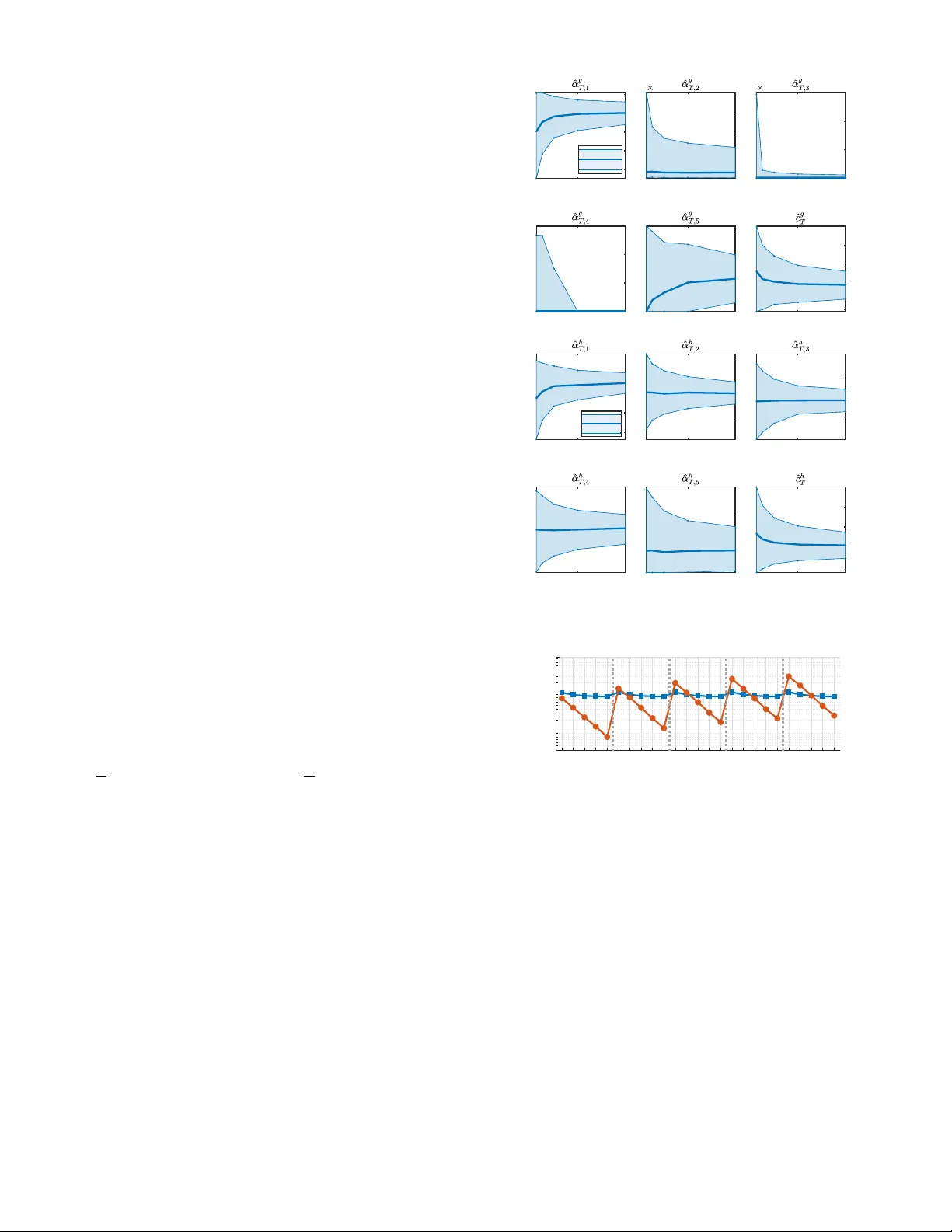
A System-Theor etic A ppr oach to Hawk es Pr ocess Identification with Guaranteed P ositivity and Stability Xinhui Rong and Girish N. Nair Abstract — The Hawkes pr ocess models self-exciting event streams, requiring a strictly non-negative and stable stochastic intensity . Standard identification methods enfor ce these prop- erties using non-negative causal bases, yielding conser vativ e parameter constraints and severely ill-conditioned least-squares Gram matrices at higher model orders. T o overcome this, we introduce a system-theoretic identification framework utilizing the sign-indefinite orthonormal Laguerre basis, which guaran- tees a well-conditioned asymptotic Gram matrix independent of model order . W e formulate a constrained least-squar es problem enfor cing the necessary and sufficient conditions for positivity and stability . By constructing the empirical Gram matrix via a L yapunov equation and repr esenting the constraints through a sum-of-squares trace equivalence, the proposed estimator is efficiently computed via semidefinite programming . I . I N T RO D U C T I O N In recent years, the unprecedented av ailability of asyn- chronous random ev ent data, arising from fields as div erse as computational neuroscience [1], genomics [2] and high- frequency finance [3], has driven a surge in neuromorphic technologies across modern robotics [4] and control systems [5]. The Hawk es process is widely regarded as the standard model for characterizing the history-dependent dynamics inherent in these ev ent-dri ven systems. A Hawk es process is defined by an intensity function that characterizes the instantaneous ev ent rate. The standard maximum likelihood estimation (MLE) [6], computed via direct gradient descent, suf fers from non-con ve xity caused by nonlinear parameters in the Hawk es impulse response (HIR). Therefore, a standard approach is to approximate the HIR using a dictionary of prescribed/user-defined causal basis functions, yielding a linear model. This facilitates the use of expectation-maximization (EM) algorithms [7], [8], [9] with explicit iterations and enables least-squares (LS) algorithms [10], [11], [12], [13] which allow for parameter constraints. Choosing suitable basis functions is a non-trivial task. The orthonormal Laguerre basis [14] is theoretically fav ored for Hawkes processes [7], [15] due to its density [16] in both L 1 [0 , ∞ ) and L 2 [0 , ∞ ) . Y et, the use of the Laguerre basis in Hawk es identification is hindered by its computational complexity and the critical requirement of a non-negati ve intensity . Consequently , the Erlang basis [7] is adopted as a con venient positive alternative with a tractable formula- tion and a guaranteed positivity through positive parameter initialization in EM algorithms [7], [8]. X. Rong ( xinhui.rong@unimelb.edu.au ) and G. N. Nair gnair@unimelb.edu.au ) are with the Department of Electrical and Electronic Engineering, Univ ersity of Melbourne, Australia. Howe ver , this loss of orthogonality incurs a sev ere nu- merical penalty in LS estimation. Our recent work [17] empirically finds that increasing the model order driv es the Hawkes-Erlang Gram matrix towards singularity . This ill- conditioning causes standard LS algorithms to fail and the asymptotic parameter error cov ariance to diver ge. Moreov er , like many other positi ve bases [18], [19], enforcing the non-negati vity of the intensity function by demanding non- negati ve parameters is merely a sufficient condition. This approach becomes increasingly conservati ve as the model order grows, excluding a vast subspace of physically valid Hawkes models. T o overcome these limitations, we model the HIR via the (sign-indefinite) orthonormal Laguerre basis and formu- late a constrained LS estimation framew ork. Our system- theoretic contributions are threefold. First, we deriv e explicit, dimension-independent bounds on the eigen v alues of the asymptotic Gram matrix for this OrthoNormal Hawk es- Laguerre (ON-HL) model, guaranteeing a well-conditioned estimator . Second, we circumvent numerical errors by com- puting the regressors and the empirical Gram matrix exactly via their continuous-time state-space realizations. Finally , we establish the necessary and sufficient conditions for a non-negati ve HIR under the ON-HL formulation. This allows us to cast the constrained LS problem as a tractable semidefinite program (SDP) that simultaneously guarantees both positivity and system stability . W e organize the paper as follows. Section II re views the Hawkes process preliminaries and Laguerre polynomial properties. Section III formulates an unconstrained centered LS problem for ON-HL identification, proving that the asymptotic Gram matrix is well-conditioned. W e also pro vide efficient computational methods for the empirical quantities via a state-space characterization. Section IV formulates the SDP problem for a positiv e and stable ON-HL model. Section V contains comparativ e simulations, and Section VI concludes the paper . All proofs are in the Appendix. I I . P R E L I M I N AR I E S W e revie w the properties of the Hawkes process and the Laguerre polynomials. W e provide the theoretical basis of the synthesis of point process statistics and systems theory . A. Hawkes Pr ocesses The Ha wkes process [20] describes history-dependent self- exciting ev ent streams, a.k.a. point pr ocesses [21]. A point process is equi valent to a counting pr ocess N t ≜ N (( −∞ , t ]) where N ( A ) counts the number of events that occur in the time set A ⊂ R . N t is a non-decreasing step function that jumps by one at each random ev ent time T r . The standard or derliness [21] condition lim δ → 0 Pr[ N ([ t,t + δ )) > 1] Pr[ N ([ t,t + δ ))=1] = 0 is in place throughour the paper The Hawkes process is characterized by a (conditional) intensity function defined as λ 0 ( t ) ≜ lim δ → 0 1 δ Pr[ N ([ t, t + δ )) = 1 |H t − ] with H t − being the history/filtration σ { N s : s < t } and the Hawkes intensity is given by λ 0 ( t ) = c 0 + χ 0 ( t ) = c 0 + Z t − −∞ ϕ 0 ( t − u ) dN u , (2.1) which is itself stochastic, describing the limiting probability rate of an increase in the counting process N conditioned on the full history H t − , and consists of a constant backgr ound rate c 0 and a stochastic memory pr ocess χ 0 ( t ) ≜ R t − −∞ ϕ 0 ( t − u ) dN u = P T r j to represent a stacked vector . W e also define S k + to be the space of real and symmetric positive definite matrices of dimension k × k . Lemma 1: [23] The orthonormal Laguerre polynomials u j ( t ) with w ( t ) = β e − β t 1 t ≥ 0 , satisty a three-term recursion u j +1 ( t ) = ( ρ j t − κ j ) u j ( t ) − γ j u j − 1 ( t ) , (2.3) with ρ j = 2 β j +1 , κ j = 2 j +1 j +1 , γ j = j j +1 , u 0 ( t ) = p 2 /β , and u j ( t ) ≜ 0 for j < 0 . As a property , 1 ρ j = γ j +1 ρ j +1 . For an arbitrary dimension m ≥ 1 , the three-term recursion takes a vector form tu m − 1 0 ( t ) = J m u m − 1 0 ( t ) + 1 ρ m − 1 u m ( t ) e m , with e m = [0 , . . . , 0 , 1] ⊤ ∈ R m and the symmetric tridiagonal Jacobi matrix J m ∈ S m + which contains κ 0 ρ 0 , · · · , κ m − 1 ρ m − 1 down its main diagonal and 1 ρ 0 , · · · , 1 ρ m − 2 down its immediate upper and lower subdiagonals. I I I . U N C O N S T R A I N E D L S F O R O N - H L This section establishes the unconstrained LS estimation using the ON-HL representation to approximate (2.1). W e theoretically show that, unlike the severely ill-conditioned Hawkes-Erlang alternative, the ON-HL asymptotic Gram matrix is inherently well-conditioned at an arbitrary model order . Finally , we deriv e an efficient system-theoretic com- putation for the empirical Gram matrix and its associated regressors. W e assume the following standard assumptions. A1: Stationarity . The true counting process N t admits the unique stationary probability measure [22] associated with the intensity (2.1) with Γ < 1 . The observed counting process ˜ N t ≜ N ((0 , t ]) is a truncation of N t within the deterministic observation period t ∈ [0 , T ] and ˜ N T ≥ 1 . A2: HIR r e gularization. The true HIR ϕ 0 satisfies (a) ϕ 0 ∈ L 1 [0 , ∞ ) ∩ L ∞ [0 , ∞ ) , and (b) R ∞ 0 tϕ 0 ( t ) dt < ∞ . The assumptions A1 and A2 are standard in the literature for asymptotic analysis [24], [22]. Under A1, the increments d ˜ N t = 1 t> 0 dN t remain strictly stationary and ergodic [25, Ch.12]. A2 ensures an almost-surely bounded intensity function and the asymptotic vanishing of the transients orig- inating from the unobserved pre-sample history [22], [17]. A2 is broadly satisfied, including mixtures of exponentials and heavy-tailed defective densities with a finite mean. A. The T runcated Hawkes Intensity A truncated intensity with a causal basis q is defined as ˜ λ q ( t ) = c + α ⊤ ˜ χ q ( t ) = c + Z t − 0 ϕ q ( t − u ; α ) d ˜ N u (3.1) ϕ q ( t ; α ) = α ⊤ q ( t ) ≥ 0 (3.2) ˜ χ q ( t ) = Z t − 0 q ( t − u ) d ˜ N u ∈ R P , (3.3) where ˜ λ q ( t ) is the P -th order truncated intensity parame- terized by the candidate background rate c > 0 and the candidate basis weights α ∈ R P . The candidate HIR ϕ q : [0 , ∞ ) 7→ [0 , ∞ ) is constructed by the prescribed causal basis q ( t ) = q P − 1 0 ( t ) ∈ R P , and ˜ χ q is the stochastic truncated memory r e gressor . The e vents before time 0 are not observed. W e propose using the ON-HL model to approximate an arbitrary Hawkes intensity (2.1) under A1, A2. Define the Laguerre basis vector h ( t ) = h P − 1 0 ( t ) = w ( t ) u ( t ) ∈ R P with u ( t ) = u P − 1 0 ( t ) ∈ R p . The truncated ON-HL intensity ˜ λ h ( t ) is defined through (3.1)-(3.3) by setting q = h . In parallel, the truncated Hawk es-Erlang intensity ˜ λ g ( t ) , currently used in the literature, is defined by replacing q in (3.1)-(3.3) by g with g ( t ) = g P − 1 0 ( t ) = w ( t ) v ( t ) ∈ R P ≥ 0 where g j ( t ) = w ( t ) v j ( t ) is the Erlang density with v j ( t ) = ( β t ) j j ! and v ( t ) = v P − 1 0 ( t ) . The Erlang basis g ( t ) = Lh ( t ) is linearly transformed from the Laguerre basis h by a lower triangular matrix L with L ij = p β / 2  i − 1 j − 1  / 2 i − 1 1 j ≤ i and ( L − 1 ) ij = p 2 /β ( − 1) i − j 2 j − 1  i − 1 j − 1  1 j ≤ i as the ( i, j ) -th component of L and L − 1 , respectively . B. The Unconstrained LS Estimator and the Asymptotics In [13], we established that the equiv alence between the unconstrained LS estimator and its centered version. W e therefore directly formulate a centered LS (CLS) estimation problem to decouple α from the background rate c to accommodate the parameter constraints to be de veloped ne xt. The CLS sets c = ˜ N T T − 1 T R T 0 α ⊤ ˜ χ q ( t ) dt with an objective 1 J q T ( α ) = 1 2 α ⊤ R q T α − α ⊤ s q T , (3.4) where s q T = 1 T R T 0 ˜ χ q ( t ) d ˜ N t − ˆ Λ T ˆ χ q T ∈ R P is the empirical cross-cov ariance with ˆ Λ T = ˜ N T T and ˆ χ q T = 1 T R T 0 ˜ χ q ( t ) dt , and the empirical Gram matrix is R q T = 1 T Z T 0 ˜ χ q ( t ) ˜ χ q ( t ) ⊤ dt − ˆ χ q T ˆ χ q ⊤ T ∈ R P × P . (3.5) Giv en that R q T is positive definite, the LS estimators are ˆ α q T = arg min α ∈ R P J q T ( α ) = ( R q T ) − 1 s q T (3.6) ˆ c q T = ˆ Λ T − ˆ χ q ⊤ T ˆ α q T , (3.7) where (3.6) follows directly from matrix calculus solving ∂ ∂ α J q T ( α ) = 0 and (3.7) recovers the centering. The following theorem on asymptotic con ver gences is a straightforward extension of an ergodic lemma developed in [17] by relaxing the positivity and unit-mass requirements for the kernel basis. W e will e valuate the conditioning of the asymptotic Gram matrix based on this theorem. A3: Basis conditions. (a) q j ∈ L 1 [0 , ∞ ) ∩ L ∞ [0 , ∞ ) , (b) R ∞ 0 t | q j ( t ) | dt < ∞ . Further, (c) for all τ > 0 , there is no pair of x  = 0 ∈ R P and d ∈ R , such that x ⊤ q ( t ) = d , almost everywhere on [0 , τ ] . Theor em 1: Suppose A1-A3 are satisfied. (a) R q T > 0 with probability one (w .p.1), so (3.6) exists and uniquely minimizes (3.4). (b) As T → ∞ , w .p.1, ˆ Λ T → Λ , ˆ χ q T → µ q , and R q T → R q ∗ ≜ E[( χ q (0) − µ q )( χ q (0) − µ q ) ⊤ ] = 1 2 π Z ∞ −∞ ¯ q ( ȷω ) ¯ C ( ω ) ¯ q ( − ȷω ) ⊤ dω ∈ S P + s q T → R ( q , 0) ∗ ≜ E[( χ q (0) − µ q )( χ 0 (0) − ΛΓ)] = 1 2 π Z ∞ −∞ ¯ q ( ȷω ) ¯ C ( ω ) ¯ ϕ 0 ( − ȷω ) ⊤ dω ∈ R P , where R q ∗ ∈ S P + is the asymptotic Gram matrix , χ q ( t ) = R t − −∞ q ( t − u ) dN u is the stationary full memory regressor with µ q ≜ E[ χ q ( t )] = Λ R ∞ 0 q ( t ) dt , and ¯ C ( ω ) = Λ | 1 − ¯ ϕ 0 ( ȷω ) | 2 is the Fourier transform of the covariance density [20] C ( u − v ) = E[ dN u dN v ] − Λ 2 dudv . 1 Heuristically , ˜ N T ≈ R T 0 ˜ λ 1 ( t ; α ) dt ⇒ c ≈ ˜ N T T − 1 T α ⊤ ˜ χ q ( t ) dt . Inserting c into the ordinary LS objective [11] results in a CLS. (c) As T → ∞ , the LS estimators ˆ α q T and ˆ c q T con verge w .p.1 to the pseudo-true values α ∗ and c ∗ , respectively: ˆ α q T → α q ∗ = ( R q ∗ ) − 1 R ( q , 0) ∗ , ˆ c q T → c q ∗ = Λ(1 − Γ q ∗ ) . Γ q ∗ = α q ⊤ ∗ R ∞ 0 q ( t ) dt is the pseudo-true branching ratio. The interpretation of the theorem is as follows. Under the A1-A3, R q T is positiv e definite w .p.1 to guarantee valid closed-form LS estimators (3.6), (3.7). R q T and s q T con verge w .p.1 to the cov ariance R q ∗ > 0 of χ q (0) and the cross- cov ariance R ( q , 0) ∗ between χ q (0) and χ 0 (0) , respectively . The asymptotic cov ariances are expressed in their spectral forms. Since R q ∗ is positiv e definite, the LS estimators con- ver ge w .p.1 to the well-defined pseudo-true parameters. W e omit the analogous definitions for the ON-HL and Hawkes- Erlang models; they respectively replace q with h and g . The following results sho w that the ON-HL model is supe- rior to the Hawkes-Erlang model in the LS setting, regarding the well-conditioning of the asymptotic Gram matrix. W e de- note the smallest and largest absolute eigenv alues of a matrix A by ρ min ( A ) and ρ max ( A ) , and the smallest and largest singular values by σ min ( A ) and σ max ( A ) , respectively . Pr oposition 1.1: Under A1, A2, Theorem 1 holds for both the Laguerre ( h ) and Erlang ( g ) bases, which satisfy A3. Pr oposition 1.2: Under A1 and A2, the asymptotic Gram matrix R h ∗ under the Laguerre basis h satisfies ρ min ( R h ∗ ) ≥ Λ (1 + Γ) 2 , ρ max ( R h ∗ ) ≤ Λ (1 − Γ) 2 , whereas under the Erlang basis g , the asymptotic Gram matrix R g ∗ satisfies R g ∗ = LR h ∗ L ⊤ , and ρ min ( R g ∗ ) ≤ ρ max ( R h ∗ ) σ 2 min ( L ) ≤ β Λ 2(1 − Γ) 2 4 − ( P − 1) ρ max ( R g ∗ ) ≥ ρ min ( R h ∗ ) σ 2 max ( L ) ≥ β Λ 2(1 + Γ) 2 . Both bases h and g satisfy A3. Under A1 and A2, while the LS estimators for both bases con ver ge w .p.1 to well-defined pseudo-true parameters, the Hawkes-Erlang model becomes numerically fragile at high model orders. The condition number of the ON-HL Gram matrix R h ∗ is upper-bounded by (1+Γ) 2 (1 − Γ) 2 , independent of P . Con versely , the Ha wkes-Erlang condition number is lower -bounded by (1 − Γ) 2 (1+Γ) 2 4 P − 1 , indicat- ing exponential ill-conditioning. Finite-precision calculations will frequently render the Erlang matrix R g T indefinite at high orders, while the Laguerre matrix R h T remains robust. The conditioning of both R h ∗ and R g ∗ inevitably worsens as Γ approaches 1 , reflecting a system near instability . C. System-Theor etic Computation of the Estimators Giv en an observation with the total number of the ob- served ev ents ˜ N T = n and the increasing ev ent times [ T 1 , · · · , T ˜ N T ] ⊤ = [ t 1 , · · · , t n ] ⊤ , we need to compute R q T and s q T for the LS estimator . While an efficient component- wise, recursi ve method [7] is a vailable for the Ha wkes-Erlang model, the computation for the ON-HL model is non-trivial. Here, we propose a system-theoretic approach for these computations, viewing the truncated memory regressors ˜ χ h as a continuous-time state space system. In what follows, ˙ f ( t ) = d f ( t ) dt | t represents the temporal deriv ative. Theor em 2: The Laguerre basis satisfies ˙ h ( t ) = Ah ( t ) with h (0) = B , where the state transition matrix A ∈ R P × P is lower -triangular with − β on the main diagonal and ( − 1) i +1 2 β on each i -th lo wer subdiagonal, and B ∈ R P has ( − 1) i +1 √ 2 β at its i -th component. Under ON-HL, ˜ χ h satisfies the stochastic differential equation (SDE) d ˜ χ h ( t ) = A ˜ χ h ( t ) dt + B d ˜ N t . (3.8) Pr oposition 2.1: Calculations of s h T and R h T follow belo w . (a) ˜ χ h ( t 1 ) = 0 , ˜ χ h ( t ( r − 1)+ ) = ˜ χ h ( t r − 1 ) + B , ˜ χ h ( t r ) = e A ( t r − t r − 1 ) ˜ χ h ( t ( r − 1)+ ) , 2 ≤ r ≤ n . (b) ˜ χ h ( T ) = e A ( T − t n ) ˜ χ h ( t n + ) , ˆ χ h T = 1 T A − 1 ( ˜ χ h ( T ) − ˜ N T B ) , ˆ Λ T = n/T , s h T = 1 T P n r =1 ˜ χ h ( t r ) − ˆ Λ T ˆ χ h T . (c) R h T solves the L yapunov equation AR h T + R h T A ⊤ + ˆ Λ T B B ⊤ + B s h ⊤ T + s h T B ⊤ + D T = 0 , where D T = 1 T ˆ χ h T ˆ χ h ⊤ T − 1 T ( ˜ χ h ( T ) − ˆ χ h T )( ˜ χ h ( T ) − ˆ χ h T ) ⊤ . The matrix A is Hurwitz by construction with all eigen- values at − β , ensuring that the L yapunov equation yields a unique, real, and symmetric solution [26] R h T . Although the indefiniteness of D T precludes a direct structural guarantee of positi ve definiteness from the equation itself, the requisite condition R h T > 0 is inherited from Theorem 1(a) and the asymptotic well-conditioning of R h ∗ in Proposition 1.2. Remark 1: Theorem 2 and Proposition 2.1 hold analo- gously for the Erlang basis, where A becomes lo wer bidiag- onal with − β on its main diagonal and β on its first lower subdiagonal, and B is sparse with β solely as its first entry . Remark 2: Under A1 and A2, as T → ∞ , D T → 0 w .p.1 [17] and the L yapunov equation becomes ( A + B α h ⊤ ∗ ) R h ∗ + R h ∗ ( A + B α h ⊤ ∗ ) ⊤ + Λ B B ⊤ = 0 , with Λ B B ⊤ ≥ 0 , R h ∗ > 0 , and ( A, B ) controllable. Then A cl = A + B α h ⊤ ∗ is Hurwitz [26]. Consequently , the pseudo-true parameter α h ∗ acts as a stabilizing state-feedback controller u ( t ) = α h ⊤ ∗ x ( t ) for the open-loop stochastic system dx ( t ) = ( Ax ( t ) + B u ( t )) dt + √ Λ B dW ( t ) , where W ( t ) is a standard Brownian motion. I V . P O S I T I V E A N D S TA B L E L S F O R O N - H L W e formulate the constrained LS for ON-HL to ensure that the identified intensity is positiv e ( ϕ h ( t ; ˆ α h T ) ≥ 0 and ˆ c h T > 0 ) and stable ( R ∞ 0 ϕ h ( t ; ˆ α h T ) dt < 1 ). Howe ver , ˆ c h T > 0 is indicated 2 by the other two conditions. Therefore, it suffices to restrain the weights α in the CLS (3.4). While the stability is enforced by a simple af fine inequality , a non-neg ativ e ON- HL HIR is guaranteed through its necessary and sufficient condition via the sum-of-squares (SOS) characterization. Lemma 2: [23] Let f be a real polynomial of degree k . f is non-negati ve on [0 , ∞ ) , iff f can be expressed as an SOS f ( t ) = a ( t ) 2 + tb ( t ) 2 , where polynomials a and b hav e maximum degrees of ⌊ k / 2 ⌋ and ⌊ ( k − 1) / 2 ⌋ , respectiv ely . 2 From (3.7), we have ˆ c h T = ˆ Λ T − ˆ χ h ⊤ T ˆ α h T , but ˆ χ h ⊤ T ˆ α h T = 1 T R T 0 R t − 0 ˆ α h ⊤ T h ( t − u ) d ˜ N u dt = 1 T R T 0 R t − 0 ϕ h ( t − u ; ˆ α h T ) d ˜ N u dt = 1 T R T 0 R T − u 0 ϕ h ( t ; ˆ α h T ) dtd ˜ N u ≤ 1 T R T 0 R ∞ 0 ϕ h ( t ; ˆ α h T ) dtd ˜ N u < ˆ Λ T . Although [23, Theorem 6] provides an SDP formulation for the SOS characterization via the eigen value decomposi- tion of the Jacobi matrix J m , this representation becomes numerically unstable at moderate model orders ( P ≈ 25 ). W e therefore implement a theoretically equiv alent trace- constrained SDP representation, ensuring robust numerical tractability even at elev ated model orders. Theor em 3: The candidate Laguerre HIR ϕ h ( t ; α ) = α ⊤ h ( t ) = w ( t ) α ⊤ u ( t ) ≥ 0 on [0 , ∞ ) iff there exist Q 1 = Q ⊤ 1 ≥ 0 ∈ R m 1 × m 1 , Q 2 = Q ⊤ 2 ≥ 0 ∈ R m 2 × m 2 with m 1 = ⌊ ( P − 1) / 2 ⌋ + 1 , m 2 = ⌊ P / 2 ⌋ , such that α j = tr { F j Q 1 } + tr { G j Q 2 } , j = 0 , 1 , · · · , P − 1 , where F j := F m 1 ,j ∈ R m 1 × m 1 and G j := G m 2 ,j ∈ R m 2 × m 2 satisfy , with the corresponding dimensions, u m − 1 0 ( t ) u m − 1 0 ( t ) ⊤ = P 2 m − 2 k =0 F m,k u k ( t ) , (4.1) tu m − 1 0 ( t ) u m − 1 0 ( t ) ⊤ = P 2 m − 1 k =0 G m,k u k ( t ) . (4.2) The constrained LS for the ON-HL model enforcing pos- itivity and stability is formulated as a con vex SDP problem with a strictly con ve x objective gi ven by min α ∈ R P ,Q 1 ,Q 2 J h T ( α ) = 1 2 α ⊤ R h T α − α ⊤ s h T subject to α j = tr { F j Q 1 } + tr { G j Q 2 } , j = 0 , · · · , P − 1 P P − 1 j =0 α j < p β / 2 Q 1 = Q ⊤ 1 ≥ 0 , Q 2 = Q ⊤ 2 ≥ 0 . Although SOS formulations for non-negati ve orthonormal polynomials are standard, this paper marks their first appli- cation to Hawkes process identification. Moreov er , the trace- based reformulation using F j and G j is fundamentally novel. Their recursiv e computations—which notably do not yield Hankel matrices as in ordinary polynomial bases (cf. [27, Ch. 2])—are detailed in the Supplementary Material [28]. V . S I M U L A T I O N S In this section, we run comprehensive simulations to compare the proposed ON-HL model and the Hawkes- Erlang model under both unconstrained and constrained LS framew orks. W e design the simulations as follows. The true intensity function λ 0 ( t ) has a background rate c 0 = 1 and the true HIR ϕ 0 ( t ) = P 3 j =1 α 0 ,j β 0 ,j e − β 0 ,j t with α 0 , 1 = α 0 , 2 = 0 . 3 , α 0 , 3 = 0 . 2 and [ β 0 , 1 , β 0 , 2 , β 0 , 3 ] ⊤ = [2 , 6 , 16] ⊤ . Thus, the true branching ratio Γ = 0 . 8 and the expected rate Λ = 5 . W e consider the observ ation period T ∈ { 50 , 100 , 200 , 400 , 800 } and simulate M = 1000 Hawkes process trajectories for each T using the thinning algorithm [29]. W e consider the model orders P ∈ { 5 , 10 , 15 , 20 , 25 } for both ON-HL and Hawkes-Erlang models with a common exponent β = 5 . W e obtain the empirical Gram matrices R h T , R g T and the cross-cov ariance estimators s h T , s g T with system iterations giv en in Proposition 2.1 and Remark 1. Unconstrained LS. First, we compare the conditioning of the empirical Gram matrices R h T and R g T . Under the Laguerre basis, R h T remains positive definite for all trajectories, upper bounded by a worst condition number of ρ max ( R h T ) ρ min ( R h T ) = 106 . 7 . In contrast, under the Erlang basis, while the matrices R g T are computed as positi ve definite for orders P ≤ 15 , around 50% and 67% of the matrices at orders P = 20 and 25 are identified as indefinite, regardless of the observation period T . The best condition numbers for the Hawkes-Erlang model across all realizations scale from 4 × 10 3 at P = 5 to an extreme 6 × 10 16 at P = 25 . W e obtain the unconstrained LS estimators ˆ α h T = ( R h T ) − 1 s h T and ˆ α g T = ( R g T ) − 1 s g T and estimate the asymptotic error covariances ˆ Σ q ( q = h or g ) by av eraging the scaled squared errors T ( ˆ α q T − α q ∗ )( ˆ α q T − α q ∗ ) ⊤ across the M = 1000 realizations at T = 800 . For the ON- HL model, the Frobenius norm ∥ ˆ Σ h ∥ F grows modestly from 3 . 6 at P = 5 to 7 . 0 at P = 25 . In contrast, the Hawkes- Erlang norm ∥ ˆ Σ g ∥ F explodes from 1 . 1 × 10 3 at P = 5 to 2 . 8 × 10 17 at P = 20 , ultimately failing at P = 25 . W e also observe that for both models, the occurrence of unstable estimators increases with the model order , and nearly 100% of the candidate HIRs become sign-indefinite when the order exceeds P = 10 , confirming the need for a constrained LS. Guaranteed Positi vity and Stability . Positivity and sta- bility are enforced via our proposed SDP for the ON-HL model, whereas the Hawkes-Erlang model uses the con- servati ve non-negativ e weights. The recursi ve computational method for F m,j and G m,j is detailed in the Supplementary Material [28]. W e implement and solve the proposed SDP us- ing the CVX package [30] in MA TLAB. All identified HIRs are strictly non-negativ e and stable. W e plot the estimator quantiles against T for model order P = 5 in Fig. 1. Under the conservati ve constraints of the Hawkes-Erlang model, the higher-order basis weights ˆ α g T ,j ( j = 2 , 3 , 4 ) are mostly zeroed out, contributing very weakly to the overall identifica- tion. Con versely , the ON-HL framew ork allows for negati ve scalar weights without violating global non-negati vity . This ensures that all basis functions remain activ e and effecti vely contribute to the LS identification. Higher model orders ( P ≥ 10 ) exhibit similar behavior; these plots are omitted for brevity . Finally , Fig. 2 plots the median squared L 2 errors, R 50 β 0 ( ϕ 0 ( t ) − ϕ h ( t ; ˆ α h T )) 2 dt and R 50 β 0 ( ϕ 0 ( t ) − ϕ g ( t ; ˆ α g T )) 2 dt to quantify the HIR approximation error . For ev ery model order P , the ON-HL model achiev es a lower approximation error than the Hawkes-Erlang model giv en a sufficiently large observation time T , indicating its superior asymptotic capabilities. Notably , the ON-HL error increases with P at smaller T , reflecting the necessary data requirements for identifying more complex parameter sets. In contrast, the Hawkes-Erlang error is completely insensitiv e to model orders, as it forces most parameters to zero. V I . C O N C L U S I O N S A N D F U T U R E W O R K W e proposed a system-theoretic identification frame work for Hawkes processes based on an orthonormal Laguerre (ON-HL) expansion. W e prov ed that the corresponding asymptotic Gram matrix is uniformly well-conditioned in the model order , whereas the Hawkes–Erlang Gram matrix be- comes e xponentially ill-conditioned. A state-space realisation yields an SDE for the Laguerre regressors and a L yapunov equation for the empirical Gram matrix, enabling efficient 50 400 800 T 0.6 0.65 0.7 0.75 0.8 Hawkes-Erlang 50 400 800 T 0 0.01 0.02 0.03 Hawkes-Erlang 50 400 800 T 0 1 2 3 4 10 -8 50 400 800 T 0 0.05 0.1 50 400 800 T 0 2 4 6 10 -7 50 400 800 T 0.8 1 1.2 1.4 10% median 90% Legend 50 400 800 T 1 1.1 1.2 1.3 1.4 ON-HL 50 400 800 T -0.2 -0.1 0 0.1 ON-HL 50 400 800 T -0.4 -0.3 -0.2 -0.1 0 50 400 800 T 0 0.05 0.1 0.15 50 400 800 T 0 0.1 0.2 0.3 0.4 50 400 800 T 0.8 1 1.2 1.4 Legend 10% median 90% Fig. 1. Quantiles of the constrained LS estimators. T50 T100 T200 T400 T800 T50 T100 T200 T400 T800 T50 T100 T200 T400 T800 T50 T100 T200 T400 T800 T50 T100 T200 T400 T800 10 -2 10 0 Squared L 2 Errors P=5 P=10 P=15 P=20 P=25 Hawkes-Erlang ON-HL Fig. 2. The squared L 2 HIR approximation errors for the constrained LS. LS computations. Using an SOS characterisation of non- negati ve polynomials, we formulated a trace-based SDP that enforces both positivity and stability of the identified inten- sity . Simulations confirmed that ON-HL maintains numerical robustness and achieves lower HIR approximation error than the Erlang-based model. In the future, we will extend the ON-HL framework to multiv ariate Hawkes processes. A . A P P E N D I X : P RO O F S Pr oof of Theorem 1. While [17, Theorem 7, Lemmas 12- 14, Theorem 15] established parallel results for a density-like basis ( q ( t ) ∈ R P ≥ 0 , R ∞ 0 q j ( t ) dt = 1 ), those strict conditions are unnecessary here. The proof that R q T > 0 relies on the Cauchy–Schwarz inequality , which does not depend on non- negati vity or unit mass of the basis. The con ver gences stated in Theorem 1 follow under the weaker assumptions stated there by in voking the ergodic lemma [17, Lemma 9] and the results on v anishing pre-sample ef fects and martingale terms in [17, Lemmas 10–11], all of which are independent of the non-negati vity condition. □ Pr oof of Proposition 1.1. Both the Erlang and Laguerre bases trivially satisfy the integral conditions A3(a)(b) be- cause polynomials are dominated by decaying exponentials. The affine independence condition A3(c) is also a conse- quence of the fundamental properties of polynomials. □ Pr oof of Pr oposition 1.2. First, use the inequalities 1 − | a | ≤ | 1 − a | ≤ 1 + | a | , a ∈ C and | ¯ ϕ 0 ( ȷω ) | = | R ∞ 0 e − ȷω t ϕ 0 ( t ) dt | ≤ R ∞ 0 ϕ 0 ( t ) dt = Γ to find Λ (1+Γ) 2 ≤ ¯ C ( ω ) ≤ Λ (1 − Γ) 2 . Since h is orthonormal, we hav e R ∞ 0 h ( t ) h ( t ) ⊤ dt = 1 2 π R ∞ 0 ¯ h ( ȷω ) ¯ h ( − ȷω ) ⊤ dω = I P , by Parse val’ s theorem. The first set of bounds for the ON-HL model follows directly . For the Erlang basis, let x − and y − be the left and right singular vectors of L corresponding to the smallest singu- lar value σ min ( L ) , respectively . By the Rayleigh quotient, ρ min ( R g ∗ ) = min ∥ x ∥ =1 x ⊤ R g ∗ x = min ∥ x ∥ =1 x ⊤ LR h ∗ L ⊤ x ≤ x ⊤ − LR h ∗ L ⊤ x − = σ 2 min ( L ) y ⊤ − R h ∗ y − ≤ σ 2 min ( L ) ρ max ( R h ∗ ) , as quoted. The counterpart for the lower bound of ρ max ( R g ∗ ) follows analogously . Further, for the lower -triangular L and L − 1 , we ha ve ρ max ( L ) = max i | L ii | = p β / 2 and ρ max ( L − 1 ) = max i | ( L − 1 ) ii | = 2 P − 1 p 2 /β . By W e yl’ s inequality , σ min ( L ) = 1 σ max ( L − 1 ) ≤ 1 ρ max ( L − 1 ) = 2 − ( P − 1) p β / 2 and σ max ( L ) ≥ ρ max ( L ) = p β / 2 . Combin- ing these bounds, the results follow . □ Pr oof of Theorem 2. Since a Laguerre basis function has a strictly proper rational L T (2.2), we find h (0) = lim s →∞ s ¯ h ( s ) = B with h j (0) = ( − 1) j √ 2 β . Rearrange the L T ratio ¯ h j ( s ) ¯ h j − 1 ( s ) = β − s β + s recursiv ely to find s ¯ h j ( s ) = − β ¯ h j ( s ) + 2 β P 0 ≤ k ≤ j − 1 ( − 1) j − k +1 ¯ h k ( s ) + ( − 1) j √ 2 β ⇒ ˙ h ( t ) = Ah ( t ) . Applying the differential operator to the con volution integral ˜ χ h ( t ) yields d ˜ χ h ( t ) = ( R t − 0 ˙ h ( t − u ) d ˜ N u ) dt + h (0) d ˜ N t = A ˜ χ h ( t ) dt + B d ˜ N t , as quoted. □ Pr oof of Pr oposition 2.1. Part (a) and the ˜ χ h ( T ) expres- sion in (b) are immediate results from the SDE (3.8). The ˆ χ h T expression follows by integrating (3.8) to find ˜ χ h ( T ) = A R T 0 ˜ χ h ( t ) dt + B ˜ N T and reorganizing with the inv ertible A . Part (c) follo ws by noting that d ( ˜ χ h ( t ) − ˆ χ h T )( ˜ χ h ( t ) − ˆ χ h T ) ⊤ = A ˜ χ h ( t )( ˜ χ h ( t ) − ˆ χ h T ) ⊤ dt + ( ˜ χ h ( t ) − ˆ χ h T ) ˜ χ h ( t ) ⊤ A ⊤ dt + B ( ˜ χ h ( t ) − ˆ χ h T ) ⊤ d ˜ N t + ( ˜ χ h ( t ) − ˆ χ h T ) B ⊤ d ˜ N t + B B ⊤ ( d ˜ N t ) 2 . Thanks to the orderliness condition, we ha ve d ˜ N t ∈ { 0 , 1 } so that ( d ˜ N t ) 2 = d ˜ N t (See [20]). Note that R h T = R T 0 ( ˜ χ h ( t ) − ˆ χ h T )( ˜ χ h ( t ) − ˆ χ h T ) ⊤ dt = R T 0 ˜ χ h ( t )( ˜ χ h ( t ) − ˆ χ h T ) ⊤ dt . Integrate both sides to get ( ˜ χ h ( T ) − ˆ χ h T )( ˜ χ h ( T ) − ˆ χ h T ) ⊤ − ˆ χ h T ˆ χ h ⊤ T = AT R h T + T R h T A ⊤ + B T s h ⊤ T + T s h T B ⊤ + B B ˜ N T . Divide through T and reorganize to get the quoted result. □ Pr oof of Theorem 3. The existence of F m,k , G m,k satis- fying (4.1), (4.2) follows from standard polynomial proper- ties. Theorem 3 follows from Lemma 2, noticing the trace identity , e.g. tr { a ( t ) } = tr { u m 1 − 1 0 ( t ) ⊤ Q 1 u m 1 − 1 0 ( t ) } = tr { u m 1 − 1 0 ( t ) u m 1 − 1 0 ( t ) ⊤ Q 1 } = P 2 m 1 − 1 k =0 tr { F m 1 ,k Q 1 } u k ( t ) . □ R E F E R E N C E S [1] W . Bialek, R. R. V an Stev eninck, F . Rieke, and D. W arland, Spikes: Exploring the Neural Code . MIT press, 1997. [2] L. Carstensen, A. Sandelin, O. Winther , and N. R. Hansen, “Multivari- ate Hawkes process models of the occurrence of regulatory elements, ” BMC Bioinformatics , vol. 11, pp. 456–474, 2010. [3] E. Bacry , I. Mastromatteo, and J.-F . Muzy , “Hawkes processes in finance, ” Mark. Micr ostruct. Liq. , vol. 1, no. 1, p. 1550005, 2015. [4] G. Gallego, T . Delbruck, G. Orchard, C. Bartolozzi, B. T aba, A. Censi, S. Leutenegger , A. J. Davison, J. Conradt, K. Daniilidis, and D. Scara- muzza, “Event-based vision: A survey , ” IEEE T rans. P attern Anal. Mach. Intell. , vol. 44, no. 01, pp. 154–180, 2022. [5] D. Shi, L. Shi, and T . Chen, Event-Based State Estimation: A Stochas- tic P erspective . New Y ork: Springer , 2015. [6] T . Ozaki, “Maximum likelihood estimation of Hawkes’ self-exciting point processes, ” Ann. Inst. Stat. Math. , vol. 31, pp. 145–155, 1979. [7] B. I. Godoy , V . Solo, and S. A. Pasha, “T runcated Hawk es point pro- cess modeling: System theory and system identification, ” Automatica , vol. 113, p. 108733, 2020. [8] E. Lewis and G. Mohler, “ A nonparametric EM algorithm for multi- scale Hawkes processes, ” J. Nonparam. Stat. , vol. 1, pp. 1–20, 2011. [9] A. V een and F . P . Schoenberg, “Estimation of space–time branching process models in seismology using an EM–type algorithm, ” J. Am. Stat. Assoc. , vol. 103, no. 482, pp. 614–624, 2008. [10] E. Bacry , M. Bompaire, S. Ga ¨ ıff as, and J.-F . Muzy , “Sparse and low- rank multivariate Hawk es processes, ” J. Machn. Learn. Res. , vol. 21, no. 50, pp. 1–32, 2020. [11] N. R. Hansen, P . Reynaud-Bouret, and V . Rivoirard, “Lasso and probabilistic inequalities for multiv ariate point processes, ” Bernoulli , vol. 21, no. 1, pp. 83–143, 2015. [12] P . Reynaud-Bouret and S. Schbath, “Adaptive estimation for Hawkes processes; application to genome analysis, ” Ann. Stat. , vol. 38, no. 5, pp. 2781 – 2822, 2010. [13] X. Rong and G. N. Nair , “On the least-squares identification for Hawkes processes, ” in Pr oc. ACC , 2026, p. in press. [14] B. W ahlberg, “System identification using Laguerre models, ” IEEE T rans. Autom. Control , vol. 36, no. 5, pp. 551–562, 1991. [15] Y . Ogata and H. Akaike, “On linear intensity models for mixed doubly stochastic poisson and self-exciting point processes, ” J. R. Stat. Soc. B , vol. 44, no. 1, pp. 102–107, 1982. [16] G. Szeg ¨ o, Orthogonal P olynomials . Rhode Island: Am. Math. Soc., 1939. [17] X. Rong and G. N. Nair , “Hawkes identification with a pre- scribed causal basis: Closed-form estimators and asymptotics, ” arXiv:2602.20795 , 2026. [18] H. Xu, M. Farajtabar , and H. Zha, “Learning Granger causality for Hawkes processes, ” in Pr oc. ICML , 2016, pp. 1717–1726. [19] K. Zhou, H. Zha, and L. Song, “Learning social infectivity in sparse low-rank networks using multi-dimensional Hawkes processes, ” in Pr oc. AIST A TS . PMLR, 2013, pp. 641–649. [20] A. G. Hawkes, “Spectra of some self-exciting and mutually exciting point processes, ” Biometrika , vol. 58, no. 1, pp. 83–90, 1971. [21] D. J. Daley and D. V ere-Jones, An intr oduction to the Theory of P oint Pr ocesses . New Y ork: Springer-V erlag, 2003. [22] P . Br ´ emaud and L. Massouli ´ e, “Stability of nonlinear Hawkes pro- cesses, ” Ann. Pr obab . , vol. 24, no. 3, pp. 1563–1588, 1996. [23] T . Roh and L. V andenberghe, “Discrete transforms, semidefinite pro- gramming, and sum-of-squares representations of nonnegativ e poly- nomials, ” SIAM J. Optim. , vol. 16, no. 4, pp. 939–964, 2006. [24] M. Eichler , R. Dahlhaus, and J. Dueck, “Graphical modeling for multiv ariate Hawkes processes with nonparametric link functions, ” J. T ime Ser . Anal. , vol. 38, no. 2, pp. 225–242, 2017. [25] D. J. Daley and D. V ere-Jones, An intr oduction to the theory of point pr ocesses: volume II: general theory and structur e . Springer Science & Business Media, 2008. [26] T . Kailath, Linear estimation . Prentice Hall, 2000. [27] B. Dumitrescu, P ositive trigonometric polynomials and signal process- ing applications , 2nd ed. Springer, 2007. [28] X. Rong and G. N. Nair, “ A system-theoretic approach to Hawkes process identification with guaranteed positi vity and stability , ” arXiv:2603.14942 , 2026. [29] Y . Ogata, “On Lewis’ simulation method for point processes, ” IEEE T rans. Inf. Theory , vol. 27, no. 1, pp. 23–31, 1981. [30] M. Grant and S. Boyd, “CVX: Matlab software for disciplined con vex programming, version 2.1, ” https://cvxr .com/cvx, Mar . 2014. **Supplementary Material: Recursive calculation for F m,k and G m,k that satisfy (4.1) and (4.2): u m − 1 0 ( t ) u m − 1 0 ( t ) ⊤ = P 2 m − 2 k =0 F m,k u k ( t ) , tu m − 1 0 ( t ) u m − 1 0 ( t ) ⊤ = P 2 m − 1 k =0 G m,k u k ( t ) . Recursive Calculation: The matrices F m,k and G m,k are the top-left block of F M ,k and G M ,k for any M > m and any k ≤ m , respectiv ely , and can be calculated recursiv ely by F m, 0 = p 2 /β I m , F m, 1 = ρ 0 ( J m − κ 0 ρ 0 I m ) F m, 0 , and F m,k +1 = ρ k ( J m − κ k ρ k I m ) F m,k − ρ k ρ k − 1 F m,k − 1 + ρ k ρ m − 1 h 0 ( m − 1) × m F ( m +1) m +1 ,k i , and G m,k = 1 ρ k − 1 F m,k − 1 + κ k ρ k F m,k + 1 ρ k F m,k +1 , where I m is an identity matrix of dimension m , and F ( m +1) m +1 ,k is the last row (the ( m + 1) -th row) of the padded matrix F m +1 ,k . Derivation: W e first find that Z ∞ 0 u m − 1 0 ( t ) u m − 1 0 ( t ) ⊤ u k ( t ) w 2 ( t ) dt = P 2 m − 2 j =0 F m,j Z ∞ 0 u j ( t ) u k ( t ) w 2 ( t ) dt = F m,k , from the definition (4.1) and the orthonormality . Thus, F m, 0 = u 0 ( t ) I m = p 2 /β I m and similarly G m,k = R ∞ 0 tu m − 1 0 ( t ) u m − 1 0 ( t ) ⊤ u k ( t ) w 2 ( t ) dt . Further , by the vector three-term recursion (2.3), we have G m,k = Z ∞ 0 tu m − 1 0 ( t ) u m − 1 0 ( t ) ⊤ u k ( t ) w 2 ( t ) dt = J m Z ∞ 0 u m − 1 0 ( t ) u m − 1 0 ( t ) ⊤ u k ( t ) w 2 ( t ) dt + 1 ρ m − 1 Z ∞ 0 e m u m ( t ) u k ( t ) w 2 ( t ) dt = J m F m,k + 1 ρ m − 1 h 0 ( m − 1) × m F ( m +1) m +1 ,k i . On the other hand, use the scalar three-term recursion in Lemma 1 to find G m,k = P 2 m − 1 j =0 F m,j Z ∞ 0 tu j ( t ) u k ( t ) w 2 ( t ) dt = 1 ρ k − 1 F m,k − 1 + κ k ρ k F m,k + 1 ρ k F m,k +1 . Reformulating the above into recursiv e formulas yields the recursiv e calculations above. In our simulations, F m,j and G m,j requires first calcu- lating the padded matrices F m 1 + P − j,j for j = 0 , 1 , . . . , P . The required F m,j and G m,j are then extracted as the top-left blocks of these padded matrices.