Hyperparameter Trajectory Inference with Conditional Lagrangian Optimal Transport

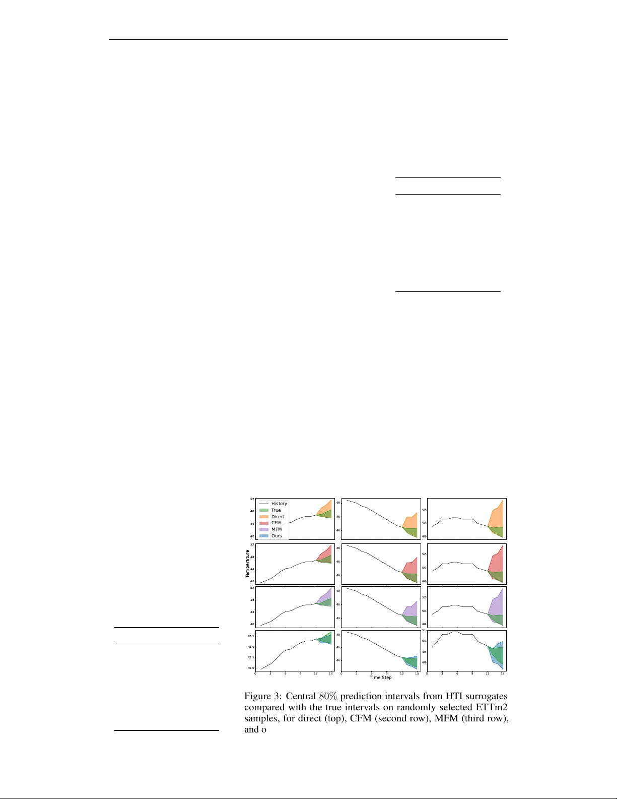
Published as a conference paper at ICLR 2026 H Y P E R P A R A M E T E R T R A J E C T O RY I N F E R E N C E W I T H C O N D I T I O N A L L A G R A N G I A N O P T I M A L T R A N S P O RT Harry Amad, Mihaela van der Schaar Department of Applied Mathematics and Theoretical Physics Univ ersity of Cambridge, UK hmka3@cam.ac.uk A B S T R AC T Neural networks (NNs) often ha ve critical behavioural trade-offs that are set at design time with hyperparameters—such as reward weights in reinforcement learn- ing or quantile tar gets in regression. Post-deployment, ho wev er, user preferences can ev olve, making initial settings undesirable, necessitating potentially expensiv e retraining. T o circumvent this, we introduce the task of Hyperparameter T rajectory Inference (HTI): to learn, from observed data, how a NN’ s conditional output distribution changes with its h yperparameters, and construct a surrogate model that approximates the NN at unobserved hyperparameter settings. HTI requires extend- ing e xisting trajectory inference approaches to incorporate conditions, e xacerbating the challenge of ensuring inferred paths are feasible. W e propose an approach based on conditional Lagrangian optimal transport, jointly learning the Lagrangian function gov erning hyperparameter-induced dynamics along with the associated optimal transport maps and geodesics between observed marginals, which form the surrogate model. W e incorporate inducti ve biases based on the manifold hypothesis and least-action principles into the learned Lagrangian, impro ving surrogate model feasibility . W e empirically demonstrate that our approach reconstructs NN outputs across various h yperparameter spectra better than other alternatives. 1 I N T R O D U C T I O N Neural network (NN) beha viour is critically shaped by hyperparameters, λ , which alter the parameters of the trained netw ork, θ λ , thereby af fecting the distribution of outputs y giv en input x , p θ λ ( y | x ) . 1 Often, hyperparameters go vern subjectiv e trade-offs, requiring users to ﬁx comple x preferences at design time. In deployment, howe ver , e volving conditions can render initial hyperparameters subop- timal, necessitating retraining, which can be infeasible. This moti vates an alternate approach—to learn a surrogate model that can sample outputs across a spectrum of h yperparameter settings. W e introduce Hyperparameter T rajectory Inference (HTI) —inspired by trajectory inference (TI) (Hashimoto et al., 2016; Lav enant et al., 2021)—to address exactly this. The goal of HTI is to learn hyperparameter-induced dynamics λ 7→ p θ λ ( y | x ) between observed distrib utions { p θ λ ( y | x ) } λ ∈ Λ obs and de velop a surrogate model ˆ p ( y | x, λ ) with which the NN conditional probability paths, for some reasonable hyperparameters λ ∈ Λ , can be estimated as ( ˆ p ( y | x, λ )) λ ∈ Λ ≈ ( p θ λ ( y | x )) λ ∈ Λ , permitting approximate inference-time adjustment of λ . Below we expand on tw o potential use cases of HTI. Reinfor cement learning. NN-based RL policies (Zhu et al., 2023; Park et al., 2025) deﬁne a state-conditional action distribution p θ λ ( a | s ) , with fundamental behaviours determined by certain hyperparameters. Consider , for instance, a policy for cancer treatment, with a reward function balancing two objectiv es: reducing tumour volume, and minimising immune system damage, weighted by a scalar λ . The ideal balance can vary per patient, based on factors such as comorbidities (Sarfati et al., 2016). An HTI surrogate polic y ˆ p ( a | s, λ ) would allo w for personalised treatment strategies, by v arying λ at inference time ( § 5.2.1). 1 p θ λ ( y | x ) = δ θ λ ( x ) ( y ) in the deterministic case, but we also consider other distributions e.g. generativ e models, or distributions parameterised by NN outputs. 1 Published as a conference paper at ICLR 2026 Quantile regr ession. Regression tasks can require measures of uncertainty . Quantile regression (K oenker & Bassett Jr, 1978) provides a way to construct prediction interv als, but typically models target individual quantiles τ , or a multi-head model outputs a ﬁxed set of quantiles (W en et al., 2018). This can make examining arbitrary quantiles, to tailor uncertainty bounds, computationally intensi ve. HTI can address this, learning the dynamics τ 7→ p θ τ ( y | x ) across a desired quantile range, yielding a surrogate that can predict all intermediate quantiles ( § 5.3). HTI is challenging, as the dynamics λ 7→ p θ λ ( y | x ) are typically non-linear , given complex deep learning optimisation landscapes (L y & Gong, 2025), making simple interpolation schemes, like conditional ﬂow matching (CFM) (Lipman et al., 2023; Liu et al., 2023; Albergo & V anden-Eijnden, 2023), unlikely to yield feasible surrogates ( ˆ p ( y | x, λ )) λ ∈ Λ . HTI requires an approach capable of capturing complex, non-Euclidean dynamics from sparse ground-truth distributions. Similar problems hav e been addressed in standard TI (T ong et al., 2020; Scarvelis & Solomon, 2023; Kapusniak et al., 2024; Pooladian et al., 2024), ho wev er the effects of conditions on probability paths, which is essential for HTI, are currently under-e xplored. W e aim to enable HTI by addressing this problem of conditional TI (CTI). W e propose an approach grounded in conditional Lagrangian optimal transport (CLOT) theory , allowing us to bias inferred conditional probability paths to remain meaningful. Speciﬁcally , we aim to learn kinetic and potential energy terms that deﬁne a Lagrangian cost function, and to encode inducti ve biases into these terms. This cost function determines what is deemed to be efﬁcient mov ement between { p θ λ ( y | x ) } λ ∈ Λ obs , and we use neural approximate solutions to the optimal transport maps and geodesics that respect this Lagrangian cost to infer conditional probability paths. W e do so in a manner inspired by Pooladian et al. (2024), extending this method to handle conditions, encode more useful inducti ve biases, and perform on more complex and higher-dimensional geometries. Once the Lagrangian and CLO T components are learned, samples for a target h yperparameter λ target ∈ Λ and condition x can be drawn by sampling from a base distribution in { p θ λ ( y | x ) } λ ∈ Λ obs , approximating CLO T maps and geodesic paths, and ev aluating the paths at the λ target position. In short, our main contributions include: 1. W e introduce the problem of Hyper parameter T rajectory Inference to enable inference-time NN behavioural adjustment, using the framing of TI to encourage particular inductiv e biases for modelling hyperparameter dynamics ( § 2.1). 2. W e propose a general method for CTI to learn comple x conditional dynamics from temporally sparse ground-truth samples, based on principles from CLOT ( § 4). W e extend the procedure of Pooladian et al. (2024) in se veral ways, learning a data-dependent potential ener gy term U alongside a kinetic term K ( § 4.1), ele vating the method to the conditional O T setting ( § 4.2), and establishing a more expressiv e neural representation for the learned metric, G θ G , underpinning K that naturally extends to higher dimensions ( § 4.3). 3. W e demonstrate empirically that our approach reconstructs conditional probability paths better than alternativ es in multiple applications of HTI, enabling effecti ve inference-time adaptation of a single hyperparameter in v arious domains ( § 5). 2 P R E L I M I N A R I E S 2 . 1 H Y P E R P A R A M E T E R T R A J E CT O RY I N F E R E N C E TI (Hashimoto et al., 2016; La venant et al., 2021) aims to recover the continuous time-dynamics t 7→ p t of a population from observed samples from a set of temporally sparse distributions { p t } t ∈T obs . CTI is an extension of TI where a conditioning v ariable x ∈ X af fects these dynamics, with a goal of inferring the conditional population dynamics t 7→ p t ( ·| x ) for arbitrary x . Building upon the concept of CTI, we introduce a nov el instantiation that we address in this work—HTI. In HTI, the ‘population’ is the outputs of a NN, with distrib ution p θ λ ( y | x ) conditioned on its input x , and we wish to learn the dynamics λ 7→ p θ λ ( y | x ) induced by a single continuous hyperparameter λ ∈ Λ (acting as ‘time’) from a set of known distrib utions { p θ λ } λ ∈ Λ obs to recov er the conditional probability paths ( p θ λ ( y | x )) λ ∈ Λ . These dynamics can be used to build a surrogate model ˆ p ( y | x, λ ) for the NN in question, allo wing efﬁcient, approximate sampling at arbitrary hyperparam- eter settings within Λ . Since many hyperparameters, by virtue of their effects during NN training, deﬁne families of NNs among which the optimal member is context dependent, such a surrogate model could reduce the need to retrain NNs in dynamic deployment scenarios. 2 Published as a conference paper at ICLR 2026 2 . 2 C O N D I T I O NA L O P T I M A L T R A N S P O RT W e deploy the frame work of conditional optimal transport (CO T) (V illani et al., 2008) to deﬁne optimal maps and paths between conditional distributions, which can be neurally approximated. Let Y 0 and Y 1 be two complete, separable metric spaces, and X be a general conditioning space. For x ∈ X , consider probability measures µ 0 ( ·| x ) ∈ P ( Y 0 ) and µ 1 ( ·| x ) ∈ P ( Y 1 ) and cost function c ( · , ·| x ) : Y 0 × Y 1 → R ≥ 0 . The primal CO T formulation (Kantorovich, 1942) in v olves a coupling π that minimises the transport cost: CO T c ( µ 0 ( ·| x ) , µ 1 ( ·| x )) = inf π ( · , ·| x ) ∈ Π( µ 0 ( ·| x ) ,µ 1 ( ·| x )) Z Y 0 ×Y 1 c ( y 0 , y 1 | x ) dπ ( y 0 , y 1 | x ) (1) where Π( µ 0 ( ·| x ) , µ 1 ( ·| x )) is the collection of all probability measures on Y 0 × Y 1 with marginals µ 0 ( ·| x ) on Y 0 and µ 1 ( ·| x ) on Y 1 . Solving this primal problem is generally intractable, and it cannot be easily neurally approximated as it requires modelling a high-dimensional joint distrib ution. The equiv alent dual formulation simpliﬁes the problem to a constrained optimisation ov er two scalar potential functions f ( ·| x ) and g ( ·| x ) : CO T c ( µ 0 ( ·| x ) , µ 1 ( ·| x )) = sup f ,g Z Y 0 f ( y 0 | x ) dµ 0 ( y 0 | x ) + Z Y 1 g ( y 1 | x ) dµ 1 ( y 1 | x ) (2) subject to the constraint f ( y 0 | x ) + g ( y 1 | x ) ≤ c ( y 0 , y 1 | x ) , ∀ ( y 0 , y 1 ) ∈ ( Y 0 , Y 1 ) . Enforcing this constraint with neural instantiations of f and g across the entire domain is challenging (Seguy et al., 2018). As such, we follow recent literature (Makkuv a et al., 2020; Amos, 2023; Pooladian et al., 2024) and utilise the semi-dual formulation based on the c -transform (V illani et al., 2008), conv erting the problem into an unconstrained optimisation ov er a single potential g ( ·| x ) : CO T c ( µ 0 ( ·| x ) , µ 1 ( ·| x )) = sup g ( ·| x ) ∈ L 1 ( µ 1 ( ·| x )) Z Y 0 g c ( y 0 | x ) dµ 0 ( y 0 | x ) + Z Y 1 g ( y 1 | x ) dµ 1 ( y 1 | x ) (3) where g c ( ·| x ) is the c -transform of g ( ·| x ) : g c ( y 0 | x ) := inf y ′ 1 ∈Y 1 { c ( y 0 , y ′ 1 | x ) − g ( y ′ 1 | x ) } . (4) Denoting g ∗ ( ·| x ) as an optimal potential for (3), the CO T map T c ( ·| x ) : Y 0 → Y 1 can be found as T c ( y 0 | x ) ∈ ar gmin y ′ 1 ∈Y 1 { c ( y 0 , y ′ 1 | x ) − g ∗ ( y ′ 1 | x ) } . (5) 2 . 3 C O N D I T I O NA L L A G R A N G I A N O P T I M A L T R A N S P O RT In the above, the cost function c is where knowledge of system dynamics can be embedded, to shape the CO T maps and paths (Asadulae v et al., 2024). The standard Euclidean cost c ( y 0 , y 1 ) = ∥ y 0 − y 1 ∥ 2 , for example, deems straight paths as the most efﬁcient. T o induce more comple x paths, gi ven our assumed comple x hyperparameter-dynamics, we require a cost function that is path-dependent, which motiv ates us to use principles from Lagrangian dynamics (Goldstein et al., 1980), bringing us to the CLO T setting. Gi ven a smooth, time-dependent curve q t for t ∈ [0 , 1] , with time deriv ativ e ˙ q t , and a Lagrangian L ( q t , ˙ q t | x ) , the action of q , S ( q | x ) , can be determined as S ( q | x ) = Z 1 0 L ( q t , ˙ q t | x ) dt. (6) The resulting Lagrangian cost function c can then be deﬁned using the least-action , or geodesic , curve between y 0 and y 1 c ( y 0 , y 1 | x ) = inf q : q 0 = y 0 ,q 1 = y 1 S ( q | x ) . (7) W e denote geodesics as q ∗ . While ﬂexible in form, a common Lagrangian instantiation is L ( q t , ˙ q t | x ) = K ( q t , ˙ q t | x ) − U ( q t | x ) = 1 2 ˙ q T t G ( q t | x ) ˙ q t − U ( q t | x ) (8) where K and U are kinetic and potential energy terms, respectively , with metric G deﬁning the geometry of the underlying manifold (e.g. for Euclidean manifolds, G = I ). W e consider learning conditional Lagrangians of the abov e form by setting a neural representation of G and estimating U using a kernel density estimate, and learning neural estimates of the transport maps and geodesics for the consequent CLO T problem. W e design U and G to incorporate biases for dense traversal and least-action into the inferred conditional probability paths. 3 Published as a conference paper at ICLR 2026 3 R E L A T E D W O R K S T rajectory inference. TI (Hashimoto et al., 2016; La venant et al., 2021) is prominent in domains such as single-cell genomics, where destructi ve measurements preclude tracking individual cells over time (Macosko et al., 2015; Schiebinger et al., 2019). Successful TI relies on le veraging inducti ve biases to generalise beyond the sparse observed times. One typical bias is based on least-action principles—assuming that populations mov e between observed mar ginals in the most efﬁcient w ay possible—naturally gi ving rise to O T approaches (Y ang & Uhler, 2019; Schiebinger et al., 2019; T ong et al., 2020; Scarvelis & Solomon, 2023; Pooladian et al., 2024). Another potential bias in vokes the manifold hypothesis (Bengio et al., 2013), which posits that data resides on a lo w-dimensional manifold, concentrated around the observ ed data (Arvanitidis et al., 2022; Chadebec & Allassonnière, 2022), to encourage inferred paths to tra verse dense regions of the data space (Kapusniak et al., 2024). Neural optimal transport. NNs hav e been used for OT , especially in high-dimensions where classical O T algorithms are infeasible (Makkuv a et al., 2020; K orotin et al., 2021). The semi-dual O T formulation with neural parametrisations of the Kantorovich potentials and transport maps is standard (Makkuv a et al., 2020; Amos, 2023; Pooladian et al., 2024). Neural CO T has also been explored (W ang et al., 2024; 2025), although with ﬁxed cost functions, and we nov elly extend this to incorporate learned conditional Lagrangian costs. Our work is particularly related to Scarvelis & Solomon (2023) and Pooladian et al. (2024), which jointly learn O T cost functions and resulting transport maps from observed time marginals. W e consider using more e xpressive forms for the cost function, in volving Lagrangians with kinetic and potential energy terms, and we operate in the conditional O T setting. Conditional generative modeling via density transport. Some generati ve models, such as condi- tional dif fusion (Ho & Salimans, 2022) and CFM models (Zheng et al., 2023), operate by transporting mass from a source to a target distrib ution, according to some condition. They can therefore be applied to conditional TI. Ho wev er , generativ e models focus on accurately learning the tar get data distribution, and the y are generally unconcerned with the intermediate distributions formed along the transport paths. While some recent works utilise O T principles to achieve more ef ﬁcient learning and sampling for CFM models (T ong et al., 2024; Pooladian et al., 2023), their primary objecti ve remains high-ﬁdelity sample generation from the target distrib ution. Bayesian optimization. Bayesian hyperparameter optimization (Snoek et al., 2012; Shahriari et al., 2015) b uilds a surrogate model of a NN’ s objecti ve function across hyperparameters. HTI extends this by learning a surrogate for the NN’ s conditional output distribution rather than for a scalar objectiv e function. HTI could allow for more ﬂexible Bayesian hyperparameter optimisation with arbitrary , post-hoc objectiv e functions calculated with surrogate samples (Appendix A). 4 N E U R A L C O N D I T I O N A L L A G R A N G I A N O P T I M A L T R A N S P O RT W e now present our method for general CTI, which inv olves a neural approach to CLO T . From ob- served temporal mar ginals, we seek to learn both the underlying conditional Lagrangian L ( q , ˙ q | x ) = K ( q , ˙ q | x ) − U ( q | x ) that governs dynamics, along with the consequent CLO T maps T c and geodesics q ∗ , such that conditional trajectories can be inferred. W e novelly encode both the inducti ve biases discussed in Section 3—least-action and dense trav ersal—into L to aid generalisation of inferred trajectories beyond the observ ed temporal regions. 4 . 1 P O T E N T I A L E N E R G Y T E R M Firstly , we set the conditional potential energy , ˆ U ( q | x ) , through which we encode a bias for dense trav ersal. By designing ˆ U ( q | x ) to be lar ge in dense regions of the data space, and small elsewhere, the Lagrangian cost function c , as in (7), will lead to geodesics that fa vour dense regions. Let D obs = { ( y i , x i , t i ) } N i =1 be the set of observ ed samples, where y i ∈ Y are the D y -dimensional ambient space observations, x i ∈ X are their D x -dimensional conditions, and t i ∈ { t 0 , t 1 , ..., t T } are the T ‘times’ of observation. W e deﬁne the potential at q ∈ Y for a given condition x ∈ X as: ˆ U ( q | x ) = α log( ˆ p ( q | x ) + ϵ ) , (9) 4 Published as a conference paper at ICLR 2026 where α > 0 is set by the user to control the strength of the density bias, ϵ > 0 is for numerical stability , and ˆ p ( q | x ) is estimated with a Nadaraya-W atson estimator (Nadaraya, 1964; W atson, 1964): ˆ p ( q | x ) = P N i =1 K h y ( q − y i ) K h x ( x − x i ) P N j =1 K h x ( x − x j ) , (10) where K h y and K h x are Gaussian kernel functions with bandwidths h y and h x , respectiv ely: K h y ( u ) = (2 π h 2 y ) − D y / 2 exp  − || u || 2 2 h 2 y  , K h x ( v ) = (2 π h 2 x ) − D x / 2 exp  − || v || 2 2 h 2 x  . (11) W e can see that (9) will be high when ˆ p ( q | x ) is high, and low when ˆ p ( q | x ) is low , thus encoding our desired bias for geodesics to trav erse dense regions of the data space. ˆ U ( q | x ) is ﬁxed throughout the subsequent learning phase for the kinetic energy term K and the CLOT maps and geodesic paths. 4 . 2 J O I N T L E A R N I N G O F K I N E T I C E N E R G Y T E R M A N D C L OT PA T H S T o learn the remaining kinetic term K ( q , ˙ q | x ) = 1 2 ˙ q T G ( q | x ) ˙ q , and solve the consequent CLO T problem, we adopt a neural approach similar to Pooladian et al. (2024), adapting it to our conditional setting. W e operate under the assumption that the observed data display dynamics that are ef ﬁcient in the underlying data manifold, to embed the desired least-action bias into our method. W e consider neural instantiations of the metric G θ G within K , and the T Kantorovich potentials g θ g,k deﬁning the CLO T problems between temporally adjacent observed distrib utions, with parameters θ G and θ g ,k respectiv ely . 2 These networks are learnt with a min-max procedure, alternating between optimising G θ G , with ﬁxed g θ g ,k , to minimise the estimated CLO T cost between observed marginals (encoding the desired least-action principles), and optimising each g θ g ,k , with ﬁxed G θ G , to maximise (3) (to accurately estimate the CLO T cost under the current metric). The overall objecti ve is min θ G X k E x  max θ g,k E y k ∼ µ k ( ·| x ) [ g c θ g,k ( y k | x )] + E y k +1 ∼ µ k +1 ( ·| x ) [ g θ g,k ( y k +1 | x )]  , (12) where µ k ( ·| x ) is the conditional distribution of the data at time t k . W e denote the inner maximisation objectiv e for each interval as L ( k ) dual ( θ g ,k ) , and the outer minimisation objectiv e as L metric ( θ G ) . Calculating g c , as in (4), requires solving an optimisation problem, with a further embedded optimi- sation problem to calculate the transport cost. These nested optimisations can make training computa- tionally infeasible. As such, we adopt the amortisation procedure from Pooladian et al. (2024), simul- taneously training and using neural approximators to output CLO T maps T θ T ,k ( y k | x ) ≈ T c,k ( y k | x ) and the parameters of a spline-based geodesic estimation, q φ ≈ q ∗ , allowing ef ﬁcient c -transform approximation. At a gi ven training iteration, the current learned map T θ T ,k warm-starts the minimisa- tion (4); this estimate is reﬁned with a limited number of L-BFGS (Liu & Nocedal, 1989) steps to yield T c,k ( y k | x ) which is used to calculcate g c in (12), and as a regression tar get for T θ T ,k : L map ( θ T ,k ) = E  ( T θ T ,k ( y k | x ) − T c,k ( y k | x )) 2  . (13) T o efﬁciently calculate the cost function required for these L-BFGS steps we approximate geodesic paths q ∗ with a cubic spline q φ , with parameters φ output by a NN S θ S trained to minimise L path ( θ S ) = E [ S ( q φ | x )] , φ = S θ S ( y k , T θ T ,k ( y k | x ) , x ) . (14) T o condition each network on x , we equip them with FiLM layers (Perez et al., 2018) that modulate the ﬁrst-layer activ ations based on x . The ov erall training procedure (Algorithm 1) alternates between updating each θ g ,k , θ T ,k , and θ s to maximise the inner part of (12), minimise (13), and minimise (14), respectiv ely , and updating θ G to minimise the outer sum in (12). 4 . 3 M E T R I C PA R A M E T R I S AT I O N W ithin the abov e procedure, the parametrisation of the neural metric G θ G is particularly important, as this must be a symmetric, positive-deﬁnite, D y -dimensional matrix to be a valid metric. Critically , 2 g θ g,k denotes the k th Kantorovich potential, for the CLO T between the distributions at t k and t k +1 5 Published as a conference paper at ICLR 2026 Algorithm 1 Neural CLO T T raining Require: Observed data D obs , ambient and conditional bandwidths h y , h x , potential weight α , no. outer training iterations N outer , no. inner training iterations N inner , learning rates η g , η T , η S , η G 1: ˆ U ( q | x ) ← α log( ˆ p ( q | x )) , where ˆ p ( q | x ) = P N i =1 K h y ( q − y i ) K h x ( x − x i ) P N j =1 K h x ( x − x j ) 2: Initialise θ G , { θ g ,k , θ T ,k } k , θ S 3: Deﬁne S ( q | x ) := R 1 0 ( 1 2 ˙ q T t G θ G ( q t | x ) ˙ q t − ˆ U ( q t | x )) dt 4: for i = 1 . . . N outer do 5: for j = 1 . . . N inner do 6: for k = 0 . . . T − 1 do 7: D k ← { ( y, x, t ) ∈ D obs | t = t k } 8: for ( y k , x ) ∈ D k do 9: y ′ k ← T θ T ,k ( y k | x ) 10: y ′∗ k ← L-BFGS ( y ′ k , S ( q ϕ | x ) − g θ g,k ( y ′ k | x )) , where ϕ = S θ S ( y k , y ′ k , x ) 11: g c θ g,k ( y k | x ) ← S ( q ϕ ∗ | x ) − g θ g,k ( y ′∗ k | x ) , where ϕ ∗ = S θ S ( y k , y ′∗ k , x ) 12: end for 13: θ g ,k ← θ g ,k + η g ∇L ( k ) dual ( θ g ,k ) , θ T ,k ← θ T ,k − η T ∇L map ( θ T ,k ) 14: end for 15: θ S ← θ S − η S ∇L path ( θ S ) 16: end for 17: θ G ← θ G − η G ∇L metric ( θ G ) 18: end for 19: return { T θ T ,k } k , S θ S there exist de generate minima to (12) by setting G θ G → 0 , where movement in all directions results in near-zero cost. W e set our parametrisation to ensure G θ G av oids this and maintains suf ﬁcient volume. In Pooladian et al. (2024), where only two-dimensional data spaces are considered, they set G θ G as a ﬁxed diagonal matrix with a neural rotation matrix G θ G ( x ) =  cos( R θ G ( x )) − sin( R θ G ( x )) sin( R θ G ( x )) cos( R θ G ( x ))   1 0 0 0 . 1   cos( R θ G ( x )) − sin( R θ G ( x )) sin( R θ G ( x )) cos( R θ G ( x ))  T (15) where R θ G ( x ) is the output of the NN. This is only applicable to two-dimensional spaces, and av oids degenerate solutions by ﬁxing the local anisotropy of G θ G . W e design a parametrisation that extends to higher dimensions, and is more expressi ve, while still a voiding degenerate solutions without requiring regularisation as in Scarvelis & Solomon (2023). Speciﬁcally , we set G θ G using its eigendecomposition G θ G = R θ G E θ G R T θ G , where a NN parametrises both a D y -dimensional diagonal matrix E θ G , and rotation matrices R θ G . T o a void de generacy , we enforce the entries of E θ G , and therefore the eigen v alues of G θ G , to be positi ve, and sum to a non-zero ‘eigen value budget’, ensuring non-tri vial volume of G θ G while permitting expressi ve levels of anisotropy . T o deﬁne the D y -dimensional rotation matrix R θ G , we multiply D y ( D y − 1) 2 Giv ens rotation matrices (Giv ens, 1958), with angles parametrised by the NN. This can impro ve performance o ver the ﬁx ed approach of Pooladian et al. (2024) in two-dimensions ( § 5.5), while also extending to higher dimensions ( § 5.3). 4 . 4 S A M P L I N G A L O N G T H E I N F E R R E D T R A J E C T O RY T o generate samples from the inferred conditional distribution ˆ p ( y | x, t ∗ ) , we use the neural approxi- mators for the CLO T maps and geodesics, a voiding the need for an y optimisation at inference time. First, samples are drawn from the ground-truth distrib ution with the largest observed base time with t k < t ∗ , y k ∼ p t k ( ·| x ) . The learned map T θ T ,k ( y k | x ) then predicts the transported point y k +1 at the end of the interv al [ t k , t k +1 ] , which contains t ∗ . Subsequently , the parameters for the approximate geodesic path q φ connecting y k to y k +1 can be estimated as φ = S θ s ( y k , y k +1 , x ) , and q φ can be ev aluated at the appropriate time. By normalising t ∗ to s ∗ = ( t ∗ − t k ) / ( t k +1 − t k ) , the inferred sample is obtained as ˆ y t ∗ = q φ ( s ∗ ) . 6 Published as a conference paper at ICLR 2026 5 E X P E R I M E N T S W e now empirically demonstrate the ef ﬁcacy of our method for CTI and some speciﬁc HTI scenarios. All results are averaged over 20 runs, and reported with standard errors. W e provide detailed experimental set-ups in Appendix C. 5 . 1 I L L U S T R A T I V E E X A M P L E O F C T I (a) K I (b) K I − ˆ U (c) K θ (d) K θ − ˆ U Figure 1: Dots represent true samples from the temporal process across t ∈ [0 , 1] , lines represent model estimated trajectories from t = 0 to t = 1 . Each condition has a distinct colour . T o illustrate our method’ s inductiv e biases, we devise a temporal process with conditions x ∈ { 1 , 2 , 3 , 4 } , where each deﬁnes a distribution p t ( y | x ) that e volves from the origin over t ∈ [0 , 1] as a noised v on Mises, with centre mo ving along one of four semicircular paths. Samples from the true process are shown in Figure 1, where each condition has a distinct colour , and lighter samples are from larger t . T o conduct CTI, using observ ations from t ∈ { 0 , 0 . 5 , 1 . 0 } , models must: (1) learn condition-dependent dynamics despite ov erlapping initial distribu- tions; (2) capture the non-Euclidean geometry of semicircular paths; and (3) generalise across t ∈ [0 , 1] from sparse temporal samples. W e compare four ablations of our method, with varying complexity of the learned conditional Lagrangian: (1) K I : Using an identity metric G = I and setting ˆ U = 0 , resulting in Euclidean geometry with no density bias; (2) K θ : Learning the metric G θ G via our method in § 4.2 and setting ˆ U = 0 , to incorporate only the inducti ve bias of least-action; (3) K I − ˆ U : Using an identity metric G = I and learning ˆ U as in § 4.1, to incorporate only the inducti ve bias of dense trav ersal, and; (4) K θ − ˆ U : Our full approach, learning both the metric G θ G and the potential term ˆ U . T able 1: NLL and CD at t ∈ { 0 . 25 , 0 . 75 } . Method NLL ( ↓ ) CD ( ↓ ) K I 105 . 713 (2 . 42) 0 . 323 (0 . 003) K θ 23 . 008 (4 . 62) 0 . 158 (0 . 009) K I − ˆ U − 0 . 532 (0 . 057) 0 . 016 (0 . 001) K θ − ˆ U − 0 . 662 (0 . 046) 0 . 016 (0 . 001) Figure 1 shows the inferred paths of samples from t = 0 to t = 1 . Our full method (Figure 1d) most faithfully reconstructs the true temporal process, as the paths correctly di verge according to their con- dition and closely follow the intended semicircular geometry . W e can see the indi vidual effects of both inductiv e biases, as individually learning ˆ U (Fig- ure 1b) results in straight paths that favour denser regions, a voiding the circle centres, while learning G θ G only (Figure 1c) better captures the underlying curv ature of the semicircular geometry . In T able 1 we ev aluate ˆ p ( y | x, t ) at withheld t ∈ { 0 . 25 , 0 . 75 } , reporting negati ve log-likelihood (NLL) and distance from the tar get circle perimeter (CD). W e can quantitativ ely see that both inducti ve biases improv e the feasibility of the inferred marginals. 5 . 2 H T I F O R R E W A R D - W E I G H T I N G I N R E I N F O R C E M E N T L E A R N I N G W e now transition to speciﬁc applications of HTI, ﬁrst addressing a compelling challenge in RL, to create surrogate policies that allo w for dynamic reward weighting. 5 . 2 . 1 C A N C E R T H E R A P Y W e in vestigate HTI for personalised cancer therapy , mirroring the ﬁrst use case presented in § 1. W e employ an en vironment from DTR-Bench (Luo et al., 2024), which we call Cancer , that simulates tumour progression under chemotherapy and radiotherapy . Natural Killer (NK) cells are pi votal immune system components, and the y can be depleted as a side ef fect of cytotoxic treatments lik e chemotherapy and radiotherap y (Shaver et al., 2021; T of foli et al., 2021), increasing susceptibility to infections and compromising treatment efﬁcac y . This side effect varies substantially with age, 7 Published as a conference paper at ICLR 2026 T able 2: A verage surrogate Cancer rew ard across λ nk ∈ { 1 , 2 , 3 , 4 , 6 , 7 , 8 , 9 } . Method Rew ard ( ↑ ) Direct − 38 . 35 (10 . 65) NLO T 9 . 26 (10 . 55) K θ 30 . 63 (8 . 50) CFM 36 . 03 (6 . 46) MFM 41 . 05 (4 . 16) K I 48 . 72 (7 . 22) K I − ˆ U 83 . 62 (5 . 37) K θ − ˆ U 102 . 49 (5 . 46) 0 2 4 6 8 10 λ N K 0 . 02 0 . 04 0 . 06 P N K T rue HTI Surrogate Figure 2: P N K vs. λ nk for ground truth policies and our surrogate policy . comorbidities, and baseline immune status (Diakos et al., 2014) and, consequently , optimal cancer therapy necessitates a patient-speciﬁc balance between tumour reduction and NK cell preserv ation. The Cancer rew ard function incorporates both tumour v olume and NK cell preservation, with a hyperparameter λ nk weighting an NK cell penalty term, P N K . Training a Proximal Polic y Optimiza- tion (PPO) (Schulman et al., 2017) agent to con ver gence in this environment tak es approximately 3 . 5 hours, so training per-patient policies with tailored λ nk is computationally prohibitiv e. This therefore presents a prime application for HTI, to enable inference-time policy adaptation. T o learn the λ nk -induced dynamics of the policy distrib ution across λ nk ∈ [0 , 10] , we train ground- truth policies with PPO at λ nk ∈ { 0 , 5 , 10 } and sample 1000 state-action pairs from each con ver ged policy , across a shared set of states, to act as the HTI training set. W e assess the four approaches from § 5.1, alongside some baselines. W e compare to: (1) a direct surrogate, where the tar get λ nk , current state, and action from λ nk = 0 are inputs to an MLP that is t rained to output actions at a gi ven λ nk via supervised regression; (2) a CFM surrogate (Lipman et al., 2023), which learns a v ector ﬁeld between the distributions at λ nk ∈ { 0 , 5 , 10 } and generates samples by inte grating actions to the desired λ nk point; (3) a metric ﬂo w matching (MFM) surrogate (Kapusniak et al., 2024) that is similar to CFM, but biases the v ector ﬁeld to point towards dense re gions of the data space; and (4) the NLO T method of Pooladian et al. (2024). W e add FiLM conditioning to these to make them appropriate for HTI. In T able 2 we report the average re ward for each surrogate at held-out λ nk ∈ { 1 , 2 , 3 , 4 , 6 , 7 , 8 , 9 } . Our full method ( K θ − ˆ U ) infers the most realistic trajectory between settings, yielding a surrogate policy with the best a verage re ward. W e also examine NK cell preserv ation in Figure 2, plotting the av erage per-episode P N K penalty for our surrogate and ground-truth policies. Our method closely mirrors the behaviour of the ground-truth policies, correctly fa vouring treatment that preserv es NK cells as λ nk increases. Critically , training our surrogate model takes approximately 15 minutes, after which rapid inference-time adaptation is possible. This contrasts with the 3 . 5 hours required to train each new PPO polic y , highlighting the substantial computational adv antage conferred by HTI. 5 . 2 . 2 R E A C H E R T able 3: A verage surro- gate Reacher re wards across λ c ∈ { 2 , 3 , 4 } . Method Rew ard ( ↑ ) Direct − 6 . 711 (0 . 070) MFM − 6 . 561 (0 . 053) K I − ˆ U − 6 . 397 (0 . 031) K I − 6 . 307 (0 . 041) CFM − 6 . 251 (0 . 028) NLO T − 6 . 173 (0 . 038) K θ − 6 . 158 (0 . 033) K θ − ˆ U − 6 . 093 (0 . 036) T o further demonstrate HTI for rew ard weighting, we ev aluate it in the Reacher en vironment from OpenAI Gym (Brockman et al., 2016), a standard continuous control benchmark. In this setting, an agent controls a two-joint arm with the goal of reaching a random target position. The re ward is designed to minimise distance to the target, while penalising the magnitude of the joint torques, discour - aging high-force movements, and it is weighted by a hyperparameter λ c . Similar to the cancer therap y experiment, we train PPO agents at λ c ∈ { 1 , 5 } , and collect 1000 state-action pairs from each agent to form the HTI training dataset. In T able 3 we ev aluate the same suite of surrogate models as pre viously , assessing inferred policy 8 Published as a conference paper at ICLR 2026 behaviour at unseen λ c ∈ { 2 , 3 , 4 } . Our full method ( K θ − ˆ U ) again yields the most performant surrogate, achie ving the highest average re ward. 5 . 2 . 3 N O N - L I N E A R R E W A R D S C A L A R I Z AT I O N T able 4: A verage surrogate Cancer_nl rew ard across λ nk ∈ { 1 , 2 , 3 , 4 , 6 , 7 , 8 , 9 } . Method Rew ard ( ↑ ) K I 42 . 84 (5 . 86) Direct 49 . 50 (17 . 90) NLO T 52 . 63 (6 . 52) K θ 54 . 44 (7 . 66) CFM 69 . 70 (7 . 73) MFM 78 . 44 (4 . 47) K I − ˆ U 86 . 21 (6 . 32) K θ − ˆ U 91 . 94 (11 . 46) The pre vious reward scalarizations inv olve linear combinations of a main objectiv e (tumour v olume/distance to tar get) and a penalty term (NK penalty/torque penalty). Such scalarization is known to lead to well-behaved trade-offs when tuning reward weights (R ˘ a- dulescu et al., 2020). For a more challenging RL setting, with less well-behav ed hyperparameter dynamics, we modify Cancer to ha ve non-linear rew ard scalarization, with a hinge penalty . In this Cancer_nl setup, the weighted NK penalty is only applied if the change in cell count crosses a threshold (see deﬁnition in Ap- pendix C.2.2). W e emplo y the same training and ev aluation protocol as in § 5.2.1, with results in T able 4. W e see that our method again achie ves the highest a verage re ward across held-out settings, remain- ing robust when the hyperparameter go verns non-linear objecti ves. 5 . 3 H T I F O R Q UA N T I L E R E G R E S S I O N W e no w demonstrate HTI’ s application in a higher -dimensional setting of quantile regression for time-series forecasting, mirroring the second use case presented in § 1. Time-series forecasting is a task where pro viding a full picture of uncertainty , such as through quantile regression, is crucial, but the need to train forecasting models to tar get distinct quantiles can hinder this. W e inv estigate whether HTI can address this by inferring intermediate quantiles from the outputs of models trained at the extremes of the quantile range. Using the ETTm2 forecasting dataset (Zhou et al., 2021), we train two MLPs to forecast a 3 -step horizon from a 12 -step history at the quantiles τ = 0 . 01 and τ = 0 . 99 , using a standard pinball loss. W e then generate a dataset of 1200 forecasts from these two models, across shared inputs, to act as the HTI training set. In T able 5 we e valuate the mean squared error (MSE) for surrogate forecasts at held-out quantiles τ ∈ { 0 . 1 , 0 . 25 , 0 . 5 , 0 . 75 , 0 . 9 } compared to the true NN outputs on unseen input data. Our full method once again outperforms all baselines. Figure 3 provides qualitati ve v alidation of this, visualising the central 80% prediction interv als (between the τ = 0 . 1 and τ = 0 . 9 quantiles) from different surrogates on a random selection of samples, alongside the 80% intervals from the ground-truth NNs. Our method most closely matches the width and shape of the true interval. T able 5: MSE of surro- gate ETTm2 forecasts compared to NNs trained across quantiles τ ∈ { 0 . 1 , 0 . 25 , 0 . 5 , 0 . 75 , 0 . 9 } . Method MSE ( ↓ ) Direct 1 . 845 (0 . 065) CFM 1 . 402 (0 . 008) MFM 1 . 387 (0 . 022) K I 0 . 765 (0 . 070) K I − ˆ U 0 . 651 (0 . 076) K θ 0 . 620 (0 . 057) K θ − ˆ U 0 . 608 (0 . 034) 40 44 48 52 History T rue Dir ect CFM MFM Ours 44 46 48 48 50 52 40 44 48 52 T emperatur e 44 46 48 48 50 52 40 44 48 52 44 46 48 48 50 52 0 3 6 9 12 15 40.0 42.5 45.0 47.5 0 3 6 9 12 15 T ime Step 44 46 48 0 3 6 9 12 15 48 49 50 51 Figure 3: Central 80% prediction interv als from HTI surrogates compared with the true intervals on randomly selected ETTm2 samples, for direct (top), CFM (second row), MFM (third row), and our (bottom) approach. 9 Published as a conference paper at ICLR 2026 5 . 4 H T I F O R D R O P O U T I N G E N E R A T I V E M O D E L L I N G T able 6: WD of surrogate two moons distributions from ground-truth diffusion mod- els, trained at dropout p ∈ { 0 . 1 , 0 . 2 , 0 . 3 , 0 . 4 , 0 . 6 , 0 . 7 , 0 . 8 , 0 . 9 } . Method WD ( ↓ ) K I 0 . 570 (0 . 020) MFM 0 . 480 (0 . 020) CFM 0 . 464 (0 . 021) Direct 0 . 450 (0 . 013) K θ 0 . 404 (0 . 018) NLO T 0 . 291 (0 . 022) K θ − ˆ U 0 . 079 (0 . 003) K I − ˆ U 0 . 060 (0 . 001) T o demonstrate a more general use case for HTI, we consider the dropout hyperparameter , which is often used for regular- isation in NN training. W e consider a simple setting, train- ing a diffusion model (Ho et al., 2020) on the sklearn two moons dataset at dropout settings p ∈ { 0 , 0 . 5 , 0 . 99 } , and we draw 1000 samples from each model to act as the HTI training set. In T able 6 we e valuate surrogate models at held-out set- tings p ∈ { 0 . 1 , 0 . 2 , 0 . 3 , 0 . 4 , 0 . 6 , 0 . 7 , 0 . 8 , 0 . 9 } , measuring the W asserstein distance (WD) between surrogate and ground-truth distributions. Our methods incorporating the density bias ˆ U perform well here, with K I − ˆ U achieving the lo west WD. W e see that HTI can be used to interpolate across a general hyper - parameter such as dropout with minimal error in this setting. 5 . 5 M E T R I C L E A R N I N G A B L A T I O N In T able 7 we compare our neural metric G θ G , with learned rotation R θ G and eigen values E θ G , against the parametrisation from Pooladian et al. (2024), which uses ﬁxed eigen v alues E . W e ev aluate both within our most expressi ve Lagrangian setting across the previous experiments with two-dimensional ambient spaces. Our parametrisation leads to better performance in most tasks, yielding a lo wer NLL in the semicircle task and higher rewards in the Cancer and Reacher en vironments. On the other hand, it achieves a slightly worse WD in the generativ e modelling droput experiment. These results suggest that it is possible to learn the eigen values of G θ G , and this can enable a more accurate recov ery of the underlying conditional dynamics. Furthermore, unlike the parametrisation of Pooladian et al. (2024), ours readily extends to higher-dimensional settings, as demonstrated in § 5.3. T able 7: G θ G ablations in 2D experiments. Semicircle Cancer Reacher Dropout G θ G NLL ( ↓ ) CD ( ↓ ) Rew ard ( ↑ ) Rew ard ( ↑ ) WD ( ↓ ) R θ G E R T θ G − 0 . 602 (0 . 033) 0 . 016 (0 . 001) 98 . 72 (6 . 32) − 6 . 122 (0 . 080) 0 . 076 (0 . 003) R θ G E θ G R T θ G − 0 . 662 (0 . 046) 0 . 016 (0 . 001) 102 . 49 (5 . 46) − 6 . 093 (0 . 036) 0 . 079 (0 . 003) 6 D I S C U S S I O N In this work, we in vestigate CTI, proposing a novel methodology grounded in the principles of CLO T . Our approach extends existing TI techniques by e xplicitly incorporating conditional information, and novelly combining dense trav ersal (via ˆ U ) and least-action (via K θ ) inductive biases. Our empirical results sho w we can eff ectively reconstruct non-Euclidean conditional probability paths from sparsely observed mar ginal distributions ( § 5.1). Our ablation study validates our neural metric parametrisation, highlighting its ability to capture intricate data geometries ( § 5.5) while extending to higher dimensions ( § 5.3). W e also in vestig ate performance at dif ferent sparsity lev els in Appendix E. Furthermore, we propose HTI as a novel and impactful instantiation of CTI, addressing the challenge of adapting NN beha viour without expensi ve retraining. W e showcased the practical utility of HTI for interpolating between rew ard weights in RL ( § 5.2), quantile targets in time-series forecasting ( § 5.3), and dropout settings in generati ve modelling ( § 5.4). For reference on the ef ﬁciency HTI can confer , the ground-truth result in Figure 2 required training 11 PPO policies, taking approximately 38 GPU hours, while the surrogate result requires training three PPO policies and an HTI surrogate, taking only 11 GPU hours. Further potential applications of HTI are discussed in Appendix A. Nev ertheless, HTI will be challenging when the underlying dynamics are chaotic, making inference from sparse samples inherently dif ﬁcult. Given the relati vely simple settings we demonstrate here, further inv estigation across a wider range of hyperparameter landscapes is warranted. Also, our method for HTI is only applicable for varying a single, continuous hyperparameter . Future work should explore e xtensions to handle multiple hyperparameters, which we discuss in Appendix D. 10 Published as a conference paper at ICLR 2026 R E P R O D U C I B I L I T Y S TA T E M E N T W e are committed to ensuring our work is reproducible. As such, we giv e a brief introduction to the mathematical concepts our method is based on in § 2, clearly describe our method in § 4, and provide concrete training and sampling algorithms in Algorithms 1 and 2, respectiv ely . For the results in § 5, we giv e detailed experimental set-ups in Appendix C. This includes detailing the datasets and en vironments used, model hyperparameters and training procedures, and pro viding references and links to ke y libraries. Furthermore, we release our code base here: https://github.com/ harrya32/hyperparameter- trajectory- inference . A C K N O W L E D G E M E N T S Harry Amad’ s studentship is funded by Canon Inc.. This work was supported by Azure sponsorship credits granted by Microsoft’ s AI for Good Research Lab . R E F E R E N C E S Michael Samuel Albergo and Eric V anden-Eijnden. Building normalizing ﬂows with stochastic interpolants. In The Eleventh International Confer ence on Learning Representations , 2023. Brandon Amos. On amortizing con ve x conjug ates for optimal transport. In The Ele venth International Confer ence on Learning Repr esentations , 2023. Georgios Arv anitidis, Miguel González-Duque, Alison Pouplin, Dimitris Kalatzis, and Søren Hauber g. Pulling back information geometry . In 25th International Confer ence on Artiﬁcial Intelligence and Statistics , 2022. Arip Asadulaev , Alexander Korotin, V age Egiazarian, Petr Mokro v , and Evgeny Burnaev . Neural optimal transport with general cost functionals. In The T welfth International Confer ence on Learning Repr esentations , 2024. Y oshua Bengio, Aaron Courville, and P ascal V incent. Representation learning: A revie w and ne w perspectiv es. IEEE transactions on pattern analysis and machine intellig ence , 35(8):1798–1828, 2013. Greg Brockman, V icki Cheung, Ludwig Pettersson, Jonas Schneider , John Schulman, Jie T ang, and W ojciech Zaremba. Openai gym. arXiv preprint , 2016. Christopher P Burgess, Irina Higgins, Arka P al, Loic Matthey , Nick W atters, Guillaume Des- jardins, and Alexander Lerchner . Understanding disentangling in beta-vae. arXiv pr eprint arXiv:1804.03599 , 2018. Clément Chadebec and Stéphanie Allassonnière. A geometric perspectiv e on variational autoencoders. Advances in Neural Information Pr ocessing Systems , 35:19618–19630, 2022. Connie I Diakos, Kellie A Charles, Donald C McMillan, and Stephen J Clarke. Cancer-related inﬂammation and treatment effecti veness. The Lancet Oncology , 15(11):e493–e503, 2014. A Ghaff ari, B Bahmaie, and M Nazari. A mixed radiotherapy and chemotherapy model for treatment of cancer with metastasis. Mathematical methods in the applied sciences , 39(15):4603–4617, 2016. W allace Giv ens. Computation of plain unitary rotations transforming a general matrix to triangular form. Journal of the Society for Industrial and Applied Mathematics , 6(1):26–50, 1958. H Goldstein, C Poole, and J Safko. Classical mechanics, 1980. Ian J Goodfello w , Jonathon Shlens, and Christian Szegedy . Explaining and harnessing adversarial examples. stat , 1050:20, 2015. T atsunori Hashimoto, David Gif ford, and T ommi Jaakkola. Learning population-lev el diffusions with generativ e rnns. In International Confer ence on Machine Learning , pp. 2417–2426. PMLR, 2016. 11 Published as a conference paper at ICLR 2026 Irina Higgins, Loic Matthey , Arka P al, Christopher Burgess, Xavier Glorot, Matthew Botvinick, Shakir Mohamed, and Alexander Lerchner . beta-vae: Learning basic visual concepts with a constrained variational frame work. In International confer ence on learning r epr esentations , 2017. Jonathan Ho and Tim Salimans. Classiﬁer-free dif fusion guidance. arXiv pr eprint arXiv:2207.12598 , 2022. Jonathan Ho, Ajay Jain, and Pieter Abbeel. Denoising diffusion probabilistic models. Advances in neural information pr ocessing systems , 33:6840–6851, 2020. Leonid V Kantorovich. On the translocation of masses. In Dokl. Akad. Nauk. USSR (NS) , volume 37, pp. 199–201, 1942. Kacper Kapusniak, Peter Potaptchik, T eodora Reu, Leo Zhang, Alexander T ong, Michael Bronstein, Joey Bose, and Francesco Di Giov anni. Metric ﬂow matching for smooth interpolations on the data manifold. Advances in Neural Information Pr ocessing Systems , 37:135011–135042, 2024. Diederik P Kingma and Max W elling. Auto-encoding v ariational bayes. stat , 1050:1, 2014. Roger K oenker and Gilbert Bassett Jr . Regression quantiles. Econometrica: journal of the Economet- ric Society , pp. 33–50, 1978. Alexander K orotin, Lingxiao Li, Aude Genev ay , Justin M Solomon, Alexander Filippo v , and Evgeny Burnaev . Do neural optimal transport solvers work? a continuous wasserstein-2 benchmark. Advances in neural information pr ocessing systems , 34:14593–14605, 2021. Hugo Lav enant, Stephen Zhang, Y oung-Heon Kim, and Geoffre y Schiebinger . T owards a mathemati- cal theory of trajectory inference. stat , 1050:18, 2021. Y aron Lipman, Ricky TQ Chen, Heli Ben-Hamu, Maximilian Nickel, and Matthew Le. Flow matching for generati ve modeling. In The Eleventh International Confer ence on Learning Repr esentations , 2023. Y aron Lipman, Marton Ha vasi, Peter Holderrieth, Neta Shaul, Matt Le, Brian Karrer , Ricky TQ Chen, David Lopez-P az, Heli Ben-Hamu, and Itai Gat. Flow matching guide and code. arXiv pr eprint arXiv:2412.06264 , 2024. Dong C Liu and Jorge Nocedal. On the limited memory bfgs method for large scale optimization. Mathematical pr ogramming , 45(1):503–528, 1989. Xingchao Liu, Chengyue Gong, et al. Flow straight and fast: Learning to generate and transfer data with rectiﬁed ﬂow . In The Eleventh International Confer ence on Learning Representations , 2023. Zhiyao Luo, Mingcheng Zhu, Fenglin Liu, Jiali Li, Y angchen Pan, Jiandong Zhou, and T ingting Zhu. Dtr-bench: an in silico en vironment and benchmark platform for reinforcement learning based dynamic treatment regime. arXiv pr eprint arXiv:2405.18610 , 2024. Andrew L y and Pulin Gong. Optimization on multifractal loss landscapes explains a di verse range of geometrical and dynamical properties of deep learning. Natur e Communications , 16(1):3252, 2025. Evan Z Macosko, Anindita Basu, Rahul Satija, James Nemesh, Karthik Shekhar , Melissa Goldman, Itay T irosh, Allison R Bialas, Nolan Kamitaki, Emily M Martersteck, et al. Highly parallel genome- wide e xpression proﬁling of individual cells using nanoliter droplets. Cell , 161(5):1202–1214, 2015. Aleksander Madry , Aleksandar Makelov , Ludwig Schmidt, Dimitris Tsipras, and Adrian Vladu. T ow ards deep learning models resistant to adv ersarial attacks. In International Conference on Learning Repr esentations , 2018. Ashok Makkuv a, Amirhossein T aghvaei, Se woong Oh, and Jason Lee. Optimal transport mapping via input con vex neural netw orks. In International Conference on Mac hine Learning , pp. 6672–6681. PMLR, 2020. 12 Published as a conference paper at ICLR 2026 Elizbar A Nadaraya. On estimating regression. Theory of Pr obability & Its Applications , 9(1): 141–142, 1964. Seohong Park, Qiyang Li, and Ser gey Levine. Flow q-learning. In International Confer ence on Machine Learning (ICML) , 2025. Ethan Perez, Florian Strub, Harm De Vries, V incent Dumoulin, and Aaron Courville. Film: V isual reasoning with a general conditioning layer . In Pr oceedings of the AAAI confer ence on artiﬁcial intelligence , v olume 32, 2018. Aram-Alexandre Pooladian, Heli Ben-Hamu, Carles Domingo-Enrich, Brandon Amos, Y aron Lipman, and Ricky T Chen. Multisample ﬂo w matching: Straightening ﬂows with minibatch couplings. ICML 2023 , 2023. Aram-Alexandre Pooladian, Carles Domingo-Enrich, Ricky T ian Qi Chen, and Brandon Amos. Neural optimal transport with lagrangian costs. In Pr oceedings of the F ortieth Confer ence on Uncertainty in Artiﬁcial Intelligence , pp. 2989–3003, 2024. Roxana R ˘ adulescu, Patrick Mannion, Diederik M Roijers, and Ann Nowé. Multi-objecti ve multi- agent decision making: a utility-based analysis and survey . Autonomous Agents and Multi-Agent Systems , 34(1):10, 2020. Antonin Rafﬁn, Ashley Hill, Adam Gleave, Anssi Kanervisto, Maximilian Ernestus, and Noah Dormann. Stable-baselines3: Reliable reinforcement learning implementations. J ournal of Machine Learning Researc h , 22(268):1–8, 2021. URL http://jmlr.org/papers/v22/ 20- 1364.html . Diana Sarfati, Bogda K oczwara, and Christopher Jackson. The impact of comorbidity on cancer and its treatment. CA: a cancer journal for clinicians , 66(4):337–350, 2016. Christopher Scarvelis and Justin Solomon. Riemannian metric learning via optimal transport. In International Confer ence on Learning Repr esentations . OpenRevie w , 2023. Geoffre y Schiebinger , Jian Shu, Marcin T abaka, Brian Cleary , V idya Subramanian, Aryeh Solomon, Joshua Gould, Siyan Liu, Stacie Lin, Peter Berube, et al. Optimal-transport analysis of single-cell gene expression identiﬁes de velopmental trajectories in reprogramming. Cell , 176(4):928–943, 2019. John Schulman, Filip W olski, Prafulla Dhariwal, Alec Radford, and Ole g Klimov . Proximal policy optimization algorithms. arXiv preprint , 2017. V ivien Seguy , Bharath Bhushan Damodaran, Remi Flamary , Nicolas Courty , Antoine Rolet, and Math- ieu Blondel. Large-scale optimal transport and mapping estimation. In ICLR 2018-International Confer ence on Learning Repr esentations , pp. 1–15, 2018. Bobak Shahriari, Ke vin Swersk y , Ziyu W ang, Ryan P Adams, and Nando De Freitas. T aking the human out of the loop: A revie w of bayesian optimization. Proceedings of the IEEE , 104(1): 148–175, 2015. Kari A Shav er, T ayler J Croom-Perez, and Alicja J Copik. Natural killer cells: the linchpin for successful cancer immunotherapy . F r ontiers in immunology , 12:679117, 2021. Jasper Snoek, Hugo Larochelle, and Ryan P Adams. Practical bayesian optimization of machine learning algorithms. Advances in neural information pr ocessing systems , 25, 2012. Elisa C T offoli, Abdolkarim Sheikhi, Y annick D Höppner , Pita de K ok, Mahsa Y azdanpanah-Samani, Jan Spanholtz, Henk MW V erheul, Hans J v an der Vliet, and T anja D de Gruijl. Natural killer cells and anti-cancer therapies: reciprocal ef fects on immune function and therapeutic response. Cancers , 13(4):711, 2021. Alexander T ong, Jessie Huang, Guy W olf, David V an Dijk, and Smita Krishnasw amy . T rajectorynet: A dynamic optimal transport network for modeling cellular dynamics. In International confer ence on machine learning , pp. 9526–9536. PMLR, 2020. 13 Published as a conference paper at ICLR 2026 Alexander T ong, Kilian Fatras, Nik olay Malkin, Guillaume Huguet, Y anlei Zhang, Jarrid Rector- Brooks, Guy W olf, and Y oshua Bengio. Improving and generalizing ﬂow-based generati ve models with minibatch optimal transport. T ransactions on Machine Learning Resear ch , pp. 1–34, 2024. Cédric V illani et al. Optimal transport: old and new , volume 338. Springer , 2008. Richard von Mises. Über die “ganzzahligkeit" der atomgewichte und v erwandete fragen. Physikalis- che Zeitsc hrift , 19:490, 1918. Jun W ang, Bohan Lei, Liya Ding, Xiao yin Xu, Xianfeng Gu, and Min Zhang. Autoencoder-based conditional optimal transport generativ e adversarial network for medical image generation. V isual Informatics , 8(1):15–25, 2024. Zheyu Oliv er W ang, Ricardo Baptista, Y oussef Marzouk, Lars Ruthotto, and Deepanshu V erma. Ef ﬁcient neural network approaches for conditional optimal transport with applications in bayesian inference. SIAM Journal on Scientiﬁc Computing , 47(4):C979–C1005, 2025. Geoffre y S W atson. Smooth regression analysis. Sankhy ¯ a: The Indian J ournal of Statistics, Series A , pp. 359–372, 1964. Ruofeng W en, Kari T orkkola, Balakrishnan Narayanaswamy , and Dhruv Madeka. A multi-horizon quantile recurrent forecaster . stat , 1050:28, 2018. KD Y ang and C Uhler . Scalable unbalanced optimal transport using generati ve adversarial networks. In International Confer ence on Learning Repr esentations , 2019. Qinqing Zheng, Matt Le, Neta Shaul, Y aron Lipman, Aditya Gro ver , and Ricky TQ Chen. Guided ﬂows for generati ve modeling and decision making. CoRR , 2023. Haoyi Zhou, Shanghang Zhang, Jieqi Peng, Shuai Zhang, Jianxin Li, Hui Xiong, and W ancai Zhang. Informer: Beyond efﬁcient transformer for long sequence time-series forecasting. In Pr oceedings of the AAAI confer ence on artiﬁcial intelligence , volume 35, pp. 11106–11115, 2021. Zhengbang Zhu, Hanye Zhao, Haoran He, Y ichao Zhong, Shenyu Zhang, Haoquan Guo, T ingting Chen, and W einan Zhang. Diffusion models for reinforcement learning: A survey . arXiv pr eprint arXiv:2311.01223 , 2023. 14 Published as a conference paper at ICLR 2026 A F U RT H E R A P P L I C AT I O N S O F H T I W e will now elaborate on some especially compelling potential applications for HTI. In general, HTI can be useful in scenarios when a user is deploying a NN in a dynamic en vironment, where behavioural preferences are context-dependent, and where the NN has a hyperparameter with a kno wn, tangible behavioural ef fect. Traditionally , in such deployment scenarios, a user would either ha ve to compromise with some ﬁxed NN beha vioural setting, determined at training time, or allo w dynamic behaviours by undergoing slo w and expensi ve retraining at dif ferent hyperparameter settings when deemed necessary . HTI can alleviate this by enabling much faster inference time NN behavioural adaptation, by sampling estimated outcomes from the surrogate model ˆ p ( y | x, λ ) for a nov el λ setting. For a visual depiction of HTI in action, see Figure 4. A . 1 V A RY I N G N E U R A L N E T W O R K R O B U S T N E S S I N DY N A M I C N O I S E S E T T I N G S Perturbations (e.g. Gaussian noise) of magnitude ϵ added to NN training data can increase rob ustness during inference for noisy inputs (Goodfello w et al., 2015; Madry et al., 2018). Calibrating the training noise to that expected to be seen in deployment can lead to optimal results in terms of inference-time accurac y . The hyperparameter ϵ directly controls this trade-off: higher ϵ typically increases robustness to noisy inputs b ut may decrease accuracy on clean data. Consider an image classiﬁcation NN used in a quality control system on a manufacturing line, where the input x image is an image of a product. The desired le vel of robustness ϵ ∗ might change based on sev eral factors: • En vironmental conditions: Changes in factory lighting can alter image noise. • Operational mode: A user might decide to temporarily increase sensitivity to minor defects (requiring lo wer ϵ ∗ for higher accurac y on subtle features) during a speciﬁc batch run, or prioritise ov erall stability (higher ϵ ∗ ) if the line is known to be e xperiencing vibrations. • Sensor age: As the camera ages, its noise proﬁle might change, warranting an adjustment to ϵ ∗ . HTI would learn a surrogate model p ( y class | x image , ϵ ) . At inference time, based on the current conditions and any explicit user preference for robustness, an appropriate ϵ ∗ can be selected. The system then samples from p ( y class | x image , ϵ ∗ ) to obtain predictions as if from a model speciﬁcally tuned for that desired robustness le vel, without needing on-the-ﬂy retraining. A . 2 V A RY I N G S H O RT - V S . L O N G - T E R M F O C U S I N R E I N F O R C E M E N T L E A R N I N G The discount factor γ ∈ [0 , 1) in reinforcement learning (RL) determines an agent’ s preference for immediate versus future rewards. A low γ leads to myopic, short-term rew ard-seeking beha viour , while a γ closer to 1 encourages far-sighted planning, v aluing future rew ards more highly . Consider an RL agent managing a patient’ s chronic disease treatment, such as T ype 2 Diabetes, where actions in volve adjusting medication dosage or recommending lifestyle interventions. The state s includes physiological markers (e.g., blood glucose le vels, HbA1c) and patient-reported outcomes. The optimal planning horizon, and thus the desired discount factor γ ∗ , can v ary based on patient preference. For example, a patient might express a desire to prioritize aggressi ve short-term glycemic control before an important impending e vent, or prefer a more conserv ativ e approach at other times when they kno w their activity will be lo w . W ith HTI, users could then adjust the desired γ ∗ based on the current clinical context. The system would then sample actions from p ( a | s, γ ∗ ) , allowing the treatment strategy to dynamically shift its focus between immediate needs and long-term objectiv es without retraining the entire RL policy for each desired γ . A . 3 V A RY I N G FI D E L I T Y A N D D I V E R S I T Y I N G E N E R A T I V E M O D E L L I N G V ariational Autoencoders (V AEs) (Kingma & W elling, 2014) are generati ve models that learn a latent representation of data. The β -V AE (Higgins et al., 2017) introduces a hyperparameter β that modiﬁes the V AE objecti ve function by weighting the Kullback-Leibler (KL) div ergence term, which acts as a regulariser on the latent space. The choice of β critically inﬂuences the model’ s behaviour: 15 Published as a conference paper at ICLR 2026 Figure 4: Example inference-time adjustment enabled by HTI. W e illustrate disparate user preferences affecting desired NN beha viour (desired λ lev el) for different users in this abstract example. Having a ﬁx ed number of trained NNs ( p θ λ i ) only allows partial exploration of the full hyperparameter trajectory , while an HTI surrogate model ( ( ˆ p ( ·| x i , λ )) λ ∈ Λ ) can estimate outputs across the entire spectrum of hyperparameters (estimated conditional probability paths represented by solid blue/red lines). Crucially , hyperparameter-induced dynamics can dif fer amongst input conditions ( x i ), as the true conditional distributions mo ve along their own respecti ve manifolds ( M x i ), so an effecti ve HTI model must learn conditional dynamics. • Low β (e.g., β < 1 ): W ith less pressure on the KL di vergence term, the model prioritizes reconstruction accurac y . This often leads to generated samples with high ﬁdelity (i.e., they closely resemble the training data and are sharp/realistic). Howe ver , the latent space might be less structured or more "entangled," potentially leading to lower diversity in no vel generations and poorer disentanglement of underlying factors of v ariation. • High β (e.g., β > 1 ): A higher β places more emphasis on making the learned latent distribution q ( z | x ) close to the prior p ( z ) (typically a standard Gaussian). This encourages a more disentangled latent space, where individual latent dimensions might correspond to distinct, interpretable factors of variation in the data (Burgess et al., 2018). While this can lead to greater diversity in generated samples and better generalisation for tasks lik e latent space interpolation, it might come at the cost of reconstruction ﬁdelity , potentially resulting in blurrier or less detailed samples as the model sacriﬁces some reconstruction capacity to satisfy the stronger regularisation. Consider a β -V AE trained to generate images. If a user needs to generate photorealistic images, a lower β ∗ would be preferred to maximise the sharpness and detail, ensuring the generated image is of high perceptual quality . On the other hand, if a user is brainstorming image ideas, a higher β ∗ would be beneﬁcial, encouraging the model to generate a wider v ariety of images and styles, e ven if indi vidual samples are slightly less photorealistic. HTI could learn a surrogate generati ve model p ( y image | z , β ) . The user could then dynamically adjust β ∗ based on their current task. A . 4 F L E X I B L E H Y P E R PA R A M E T E R O P T I M I S A T I O N W I T H B A Y E S I A N O P T I M I S A T I O N Standard Bayesian Optimization (BO) (Snoek et al., 2012; Shahriari et al., 2015) typically in volv es learning a probabilistic surrogate model for a speciﬁc scalar objective function f : Λ → R (e.g., validation accuracy). This creates a rigid dependency: if the user’ s preference changes during deployment—for instance, shifting from maximising pure accuracy to maximising accurac y subject to a fairness constraint or an inference latency budget—the learned surrogate is no longer v alid for the new objecti ve, and the hyperparameter search process must be restarted. HTI can decouple the surrogate model from the objecti ve function. Because HTI learns a surrogate for p θ λ ( y | x ) rather than a scalar objecti ve, it can be used to calculate any performance metric deriv ed from the model outputs as so: 16 Published as a conference paper at ICLR 2026 1. The HTI model is trained on a sparse set of anchor models to learn the conditional probability paths. 2. Post-training, a user can deﬁne an arbitrary objecti ve function J ( λ ) based on the model outputs (e.g., Expected Calibration Error , F1-score, or a custom utility function balancing risk and rew ard). 3. A BO optimiser searches for the optimal λ ∗ that minimises J ( λ ) by querying the HTI surrogate ˆ p ( y | x, λ ) . Critically , ev aluating the objecti ve J via the HTI surrogate is much faster than retraining the original neural network. This could allow users to e xplore arbitrary Pareto frontiers of competing objectiv es without the need for further expensi ve ground-truth model training, or training multiple surrogate objectiv es as in standard BO. 17 Published as a conference paper at ICLR 2026 B S A M P L I N G A L G O R I T H M W e summarise our sampling procedure, as detailed in § 4, below in Algorithm 2. Algorithm 2 Sampling from ˆ p ( y | x, t ∗ ) Require: T rue distributions { p t k ( ·| x ) } t k ∈T obs , CLO T maps { T θ T ,k } k , geodesic path generator S θ S , target mar ginal t ∗ , condition x ∈ X Find k such that t k , t k +1 ∈ T obs and t k < t ∗ < t k +1 . y k ∼ p t k ( ·| x ) . ˆ y k +1 = T θ T ,k ( y k | x ) Deﬁne spline geodesic path q φ ( · ) with φ = S θ S ( y k , ˆ y k +1 , x ) s ∗ = ( t ∗ − t k ) / ( t k +1 − t k ) . ▷ Normalise target mar ginal for current interval ˆ y t ∗ = q φ ( s ∗ ) retur n ˆ y t ∗ 18 Published as a conference paper at ICLR 2026 C E X P E R I M E N T A L D E TA I L S W e now provide detailed experimental set-ups for each of our experiments in § 5. The code implementation of our method is included here: https://github.com/harrya32/ hyperparameter- trajectory- inference . W e ran all e xperiments on an Azure VM A100 GPU. A single run for the semicircles experiment took between 5-10 minutes, depending on the surrogate model. T o produce data for the re ward-weighting experiments, it took 3.5 hours to train a PPO agent at each setting. For the cancer experiment, it took between 2-15 minutes to train the surrogate models. For the reacher experiment, it took between 1-7 minutes to train the surrogate models. For the quantile regression experiment, it took approximately 5 minutes to train the MLP quantile forecasters, and between 2-15 minutes to train the surrogate models. F or the generativ e modelling dropout experiment, it took between 6-20 minutes to train the surrogate models. Ultimately , ﬁnal e xperimental runs inv olve approximately 120 GPU hours of training time. W e base the implementation of our method off the code from Pooladian et al. (2024) (CC BY -NC 4.0 License, https://github.com/facebookresearch/lagrangian- ot ), which we adapt for our speciﬁc setting. C . 1 S E M I C I R C L E S E X P E R I M E N T C . 1 . 1 S E M I C I R C L E S D A TA S E T W e describe here the temporal process we used to generate the conditional semicircles synthetic dataset from § 5.1. The dataset comprises 2D points ( x, y ) associated with one of four discrete conditions c ∈ { 1 , 2 , 3 , 4 } , generated at a continuous time t ∈ [0 , 1] . For each condition and time, points are generated by ﬁrst sampling an angle from a V on Mises distribution (v on Mises, 1918), with a time- and condition-dependent mean, and then sampling a radius from a Log-Normal distribution centred around a unit circle radius. Speciﬁcally , the generation process for a single point under condition c at time t is as follows: Global parameters: • r nom = 1 : Nominal radius of the semicircles. • σ rad = 0 . 05 : Standard deviation of the logarithm of the radial component, controlling radial spread. • κ ang = 5 . 0 : Angular concentration parameter for the V on Mises distribution. Generation: For each condition c and time t : 1. Sample radius ( R ): The radial component R is drawn from a Log-Normal distrib ution, such that log( R ) is normally distrib uted: log( R ) ∼ N ( µ log , σ 2 log ) where µ log = log( r nom ) and σ log = σ rad . Thus, R ∼ LogNormal (log ( r nom ) , σ 2 rad ) This distribution is independent of condition c and time t . 2. Mean angle ( µ ang ( c, t ) ) and semicir cle centre ( x offset ,c ): The mean angle µ ang ( c, t ) and the x-coordinate of the semicircle’ s center x offset ,c are determined by the condition c and time t : x offset ,c =  − 1 . 0 if c ∈ { 1 , 2 } 1 . 0 if c ∈ { 3 , 4 } µ ang ( c, t ) =        tπ if c = 1 ( top-left semicircle, 0 → π ) − tπ if c = 2 ( bottom-left semicircle, 0 → − π ) (1 − t ) π if c = 3 ( top-right semicircle, π → 0) ( t − 1) π if c = 4 ( bottom-right semicircle, − π → 0) 19 Published as a conference paper at ICLR 2026 3. Sample angle ( Φ c ( t ) ): The angular component Φ c ( t ) is drawn from a V on Mises distribution centred at the mean angle: Φ c ( t ) ∼ V onMises ( µ ang ( c, t ) , κ ang ) 4. Cartesian coordinates ( x c ( t ) , y c ( t ) ): The 2D coordinates are obtained by con verting the sampled polar coordinates ( R, Φ c ( t )) to Cartesian, relativ e to the semicircle’ s center: x c ( t ) = x offset ,c + R cos(Φ c ( t )) y c ( t ) = R sin(Φ c ( t )) The full dataset at a given time t consists of N samples drawn from each of the four conditional distributions. In § 5.1 and § 5.5 our training data consists of 100 samples for each condition at times t ∈ { 0 , 0 . 5 , 1 . 0 } . The geodesics plotted in Figure 1 begin at true points sampled at t = 0 and end at their estimated CLO T maps at t = 1 . For the numerical results in T ables 1 and 7, we compare estimated distrib utions from the respectiv e models to the true distributions at t ∈ { 0 . 25 , 0 . 75 } . C . 1 . 2 M O D E L D E TA I L S The hyperparameters for the surrogate models used in the semicircles experiments are listed in T able 8. Note that, since we ha ve discrete conditions in this e xperiment, we construct separate NW density estimators for each condition, hence we set h x as N/A. Hyperparameter V alue α 0 . 05 for models with ˆ U , 0 otherwise h y 0 . 05 h x N/A Epochs 2001 G θ G learning rate 5 × 10 − 3 G θ G MLP hidden layer sizes [128 , 128] G θ G activ ations ReLU G θ G eigen value b udget 2 g θ g , T θ T MLP hidden layer sizes [64 , 64 , 64 , 64] S θ S MLP hidden layer sizes [1024 , 1024] g θ g , T θ T , S θ S learning rate 10 − 4 g θ g , T θ T , S θ S activ ations ReLU Spline knots 15 FiLM layer size (applied to ﬁrst layer activ ations) 16 c -T ransform solver LBFGS, 10 iterations Min-max optimisation 1 × G θ G update per 10 × g θ g , T θ T , S θ S updates T able 8: Hyperparameters for semicircle experiments in § 5.1. C . 2 C A N C E R T H E R A P Y E X P E R I M E N T C . 2 . 1 E N V I R O N M E N T W e conduct this e xperiment using the ‘Ghaf fariCancerEn v-continuous’ en vironment from DTR-Bench / DTR-Gym (Luo et al., 2024) ( https://github.com/GilesLuo/DTRGym , MIT license) which is based on the mathematical model for treatment of cancer with metasta- sis using radiotherapy and chemotherapy proposed in Ghaf fari et al. (2016). The implementation deviates from Ghaffari et al. (2016) by treating the dynamics of circulating lymphocytes ( c 1 ) and tumor-inﬁltrating c ytotoxic lymphocytes ( c 2 ) as constant. The state at time t is an 8-dimensional continuous vector representing k ey biological and treatment- related quantities: S t = [ T p,t , N p,t , L p,t , C t , T s,t , N s,t , L s,t , M t ] T where: 20 Published as a conference paper at ICLR 2026 • T p,t : T otal tumour cell population at the primary site. • N p,t : Concentration of Natural Killer (NK) cells at the primary site (cells/L). • L p,t : Concentration of CD8+T cells at the primary site (cells/L). • C t : Concentration of lymphocytes in blood (cells/L). • T s,t : T otal tumour cell population at the secondary (metastatic) site. • N s,t : Concentration of NK cells at the secondary site (cells/L). • L s,t : Concentration of CD8+T cells at the secondary site (cells/L). • M t : Concentration of chemotherapy agent in the blood (mg/L). All state components are non-negati ve real v alues. The action at time t is a 2-dimensional continuous vector representing the treatment intensities: A t = [ D t , v t ] T where: • D t : The effect of radiotherapy applied at time t . • v t : The effect of chemotherapy applied at time t . These actions inﬂuence the dynamics of the state v ariables according to the underlying mathematical ODE model. The rew ard R t receiv ed after taking action A t in state S t and transitioning to state S t +1 is designed to encourage tumor reduction while penalizing signiﬁcant deviations in Natural Killer (NK) cell populations, with an additional re ward or penalty in terminal states. Let S 0 = [ T p, 0 , N p, 0 , . . . ] T be the initial state of an episode. The components of the reward at each non-terminal step are: T umor r eduction component ( R tumor ): This component measures the relativ e reduction in total tumor cells. First, the total tumor populations at the current step k (representing S t +1 ) and at the initial step 0 are calculated: T tot ,k = T p,k + T s,k and T tot , 0 = T p, 0 + T s, 0 These are then log-transformed: T k = ln(max( e, T tot ,k )) and T 0 = ln(max( e, T tot , 0 )) The tumor reduction rew ard is then: R tumor ,t = 1 − T t +1 T 0 NK cell population penalty ( R nk ): This component penalizes deviations of the total NK cell population from its initial value. The total NK cell populations are: N tot ,k = N p,k + N s,k and N tot , 0 = N p, 0 + N s, 0 These are also log-transformed: N k = ln(max( e, N tot ,k )) and N 0 = ln(max( e, N tot , 0 )) The penalty is then calculated, with weighting factor λ nk : R nk ,t = − λ nk     N t +1 N 0 − 1     Finally , a termination reward ( R term ) is added if the episode ends: R term =    100 if positiv e termination (no more tumour) − 100 if negati ve termination (max tumour size) 0 if non-terminal step The total rew ard at step t is: R t = R step ,t + R term =  1 − T t +1 T 0  − λ nk     N t +1 N 0 − 1     + R term 21 Published as a conference paper at ICLR 2026 C . 2 . 2 N O N - L I N E A R R E W A R D V A R I A N T : For the non-linear rew ard scalarization experiment ( § 5.2.3), denoted as Cancer_nonlin , we modify the re ward function to incorporate a hinge mechanism on the NK penalty term, employing the non-linear reward scalarization discussed in eq. (6) in (R ˘ adulescu et al., 2020). In this setting, the weighted NK cell penalty is only active if the relati ve de viation exceeds a threshold of 0 . 01 . The modiﬁed penalty term R nk ,t is deﬁned as: R nk ,t = ( − λ nk    N t +1 N 0 − 1    if    N t +1 N 0 − 1    > 0 . 01 0 otherwise All other components of the rew ard function remain unchanged. C . 2 . 3 P O L I C I E S W e train PPO agents (Schulman et al., 2017) for the true distrib utions p θ λ ( a | s ) at various λ nk settings using the implementation in Stable Baselines3 (Rafﬁn et al., 2021) (MIT license, https://github.com/DLR- RM/stable- baselines3 ), with all other hyperparameters left at default, using the MLPPolicy architecture. For each agent, we train for 500 , 000 timesteps. Once trained, we use samples from the models with λ nk ∈ { 0 , 5 , 10 } as the training dataset for each surrogate model. Speciﬁcally , we run the agent with λ nk = 10 for 100 steps in the environment, collecting 10 actions from each (stochastic) polic y per observ ation. W e e valuate each surrogate model at λ nk ∈ { 1 , 2 , 3 , 4 , 6 , 7 , 8 , 9 } . C . 2 . 4 M O D E L D E TA I L S The hyperparameters for our surrogate models for the adapti ve re ward-weighting experiment are listed in T able 9. Hyperparameter V alue α 0 . 01 for models with ˆ U , 0 otherwise h y 1 . 0 h x 1 . 0 Epochs 2001 G θ G learning rate 5 × 10 − 3 G θ G MLP hidden layer sizes [128 , 128] G θ G activ ations ReLU G θ G eigen value b udget 2 g θ g , T θ T MLP hidden layer sizes [64 , 64 , 64 , 64] S θ S MLP hidden layer sizes [1024 , 1024] g θ g , T θ T , S θ S learning rate 10 − 4 g θ g , T θ T , S θ S activ ations ReLU Spline knots 15 FiLM layer size (applied to ﬁrst layer activ ations) 16 c -T ransform solver LBFGS, 3 iterations Min-max optimisation 1 × G θ G update per 10 × g θ g , T θ T , S θ S updates T able 9: Hyperparameters for our surrogate models in the cancer therapy e xperiment in § 5.2.1 and § 5.2.3. For the direct surrogate model, we train a four -layer MLP using supervised learning, with inputs of the base action, condition, and target h yperparameter, and output of the target action at the rele vant hyperparameter setting. W e list the direct surrogate hyperparameters in T able 10. For the CFM surrog ate model (Lipman et al., 2023), we train two ﬂo w matching models, to model the vector ﬁelds between the distrib utions at λ nk = 0 and λ nk = 5 , and between λ nk = 5 and λ nk = 10 respectiv ely . W e base our implementation on the open source code from Lipman et al. (2024), found here: https://github.com/facebookresearch/flow_matching (CC BY -NC 22 Published as a conference paper at ICLR 2026 Hyperparameter V alue Epochs 10000 Early stopping patience 100 V alidation set 10% Batch size 256 Learning rate 10 − 3 Hidden layer sizes [64 , 64 , 64 , 64] Activ ation function Swish FiLM layer size (applied to ﬁrst layer activ ations) 16 T able 10: Hyperparameters for the direct surrogate model in the cancer therapy experiment in § 5.2.1. 4.0 License). W e extend this implementation to incorporate external conditions via a FiLM layer . The hyperparameters for both of the CFM models in this surrogate model are listed in T able 11. Hyperparameter V alue Epochs 10000 Early stopping patience 100 V alidation set 10% Batch size 1000 Learning rate 10 − 3 Hidden layer sizes [64 , 64 , 64 , 64] Activ ation function Swish FiLM layer size (applied to ﬁrst layer activ ations) 16 T able 11: Hyperparameters for the CFM surrogate model in the cancer treatment experiment in § 5.2.1. For the MFM surrogate model, we base our implementation on the open source code from Kapusniak et al. (2024), found here: https://github.com/kkapusniak/ metric- flow- matching (MIT License). This method is similar to ﬂo w matching, howe ver it aims to learn a vector ﬁeld that leads to interpolants staying on the data manifold deﬁned by the observed data. It does so by learning a NN-based correction to the straight line interpolants used in CFM training, that is designed to minimise the transport cost associated with a data-dependent Riemannian metric. These corrected interpolants are then used to train a neural vector ﬁeld. For the data-depended metric, we use their LAND formulation, which sets a diagonal metric G LAND ( x ) = diag ( h ( x ) + εI ) − 1 , where h α ( x ) = N X i =1 ( x α i − x α ) 2 exp( − || x − x i || 2 2 σ 2 ) , (16) with kernel size σ . W e extend the original implementation to incorporate external conditions via a FiLM layer in both the NN-based interpolant correction, and the neural v ector ﬁeld. The hyperparameters we use for the MFM method are listed in T able 12. For the NLO T surrogate model, this is equiv alent to our method, b ut setting ˆ U = 0 and using the ﬁxed eigen value metric from Pooladian et al. (2024). W e use the same hyperparameters as our surrogate models for this method. 23 Published as a conference paper at ICLR 2026 Hyperparameter V alue Epochs 2000 Early stopping patience 100 V alidation set 10% Batch size 128 Interpolant learning rate 10 − 4 V ector ﬁeld learning rate 10 − 3 Interpolant hidden layer sizes [64 , 64 , 64] V ector ﬁeld hidden layer sizes [64 , 64 , 64] Activ ation function SELU FiLM layer size (applied to ﬁrst layer activ ations) 16 ε 0.001 α 1 σ 3 T able 12: Hyperparameters for the MFM surrogate model in the cancer treatment experiment in § 5.2.1. C . 3 R E A C H E R C . 3 . 1 E N V I R O N M E N T W e conduct this experiment using the Reacher-v2 en vironment from OpenAI Gym ( https: //github.com/openai/gym , MIT License). This en vironment consists of a two-jointed robotic arm where the goal is to mov e the arm’ s end-effector to a randomly generated tar get location. The state at time t is an 11-dimensional continuous vector representing the angles and v elocities of the arm’ s joints, as well as the location of the tar get and the vector from the ﬁngertip to the target: S t = [cos( θ 1 ) , cos( θ 2 ) , sin( θ 1 ) , sin( θ 2 ) , x target , y target , ˙ θ 1 , ˙ θ 2 , x ﬁngertip − x target , y ﬁngertip − y target , z ﬁngertip − z target ] T where: • cos( θ 1 ) , cos( θ 2 ) : Cosine of the angles of the two joints. • sin( θ 1 ) , sin( θ 2 ) : Sine of the angles of the two joints. • x target , y target : The x and y coordinates of the target location. • ˙ θ 1 , ˙ θ 2 : The angular velocities of the two joints. • x ﬁngertip − x target , y ﬁngertip − y target , z ﬁngertip − z target : The vector from the ﬁngertip to the tar get. The action at time t is a 2-dimensional continuous vector representing the torque applied to the two joints: A t = [ τ 1 , τ 2 ] T and each τ i ∈ [ − 1 , 1] . The reward R t receiv ed at each step is the sum of a distance-to-target re ward and a control cost penalty: R t = −∥  p ﬁngertip ,t +1 −  p target ∥ 2 − λ control ∥  a t ∥ 2 2 where the ﬁrst term is the ne gativ e Euclidean distance between the ﬁngertip and the tar get, and the second is the ne gative squared Euclidean norm of the action v ector , which penalises large torques. W e introduce the weighting hyperparameter , λ control , that controls the strength of the control penalty in the rew ard. C . 3 . 2 P O L I C I E S W e train PPO agents (Schulman et al., 2017) at the setting λ control ∈ { 1 , 2 , 3 , 4 , 5 } using the im- plementation in Stable Baselines3 (Rafﬁn et al., 2021) (MIT license, https://github. 24 Published as a conference paper at ICLR 2026 com/DLR- RM/stable- baselines3 ). W e use the MLPPolicy architecture with default hy- perparameters. Each agent is trained for 1 , 000 , 000 total timesteps. Once trained, we use samples from the models with λ control ∈ { 1 , 5 } as the training dataset for our surrogate model ˆ p ( a | s, λ ) . Speciﬁcally , we run the agent with λ control = 1 for 1000 steps in the en vironment, collecting actions from each policy per observation. W e ev aluate each surrogate model at λ control ∈ { 2 , 3 , 4 } . C . 3 . 3 M O D E L D E TA I L S The hyperparameters for our surrogate models for the Reacher experiment are listed in T able 13. Hyperparameter V alue α 0 . 001 for models with ˆ U , 0 otherwise h y 2 . 0 h x 1 . 0 Epochs 2001 G θ G learning rate 5 × 10 − 3 G θ G MLP hidden layer sizes [128 , 128] G θ G activ ations ReLU G θ G eigen value b udget 2 g θ g , T θ T MLP hidden layer sizes [64 , 64 , 64 , 64] S θ S MLP hidden layer sizes [1024 , 1024] g θ g , T θ T , S θ S learning rate 10 − 4 g θ g , T θ T , S θ S activ ations ReLU Spline knots 15 FiLM layer size (applied to ﬁrst layer activ ations) 16 c -T ransform solver LBFGS, 3 iterations Min-max optimisation 1 × G θ G update per 10 × g θ g , T θ T , S θ S updates T able 13: Hyperparameters for reacher experiment in § 5.2.2. For the direct surrogate model, we train a four -layer MLP in the same fashion as the cancer therapy experiment, with the same hyperparameters (T able 10). For the CFM surrogate model, we train one ﬂow matching model, between the distrib utions at λ control = 1 and λ control = 5 with the same hyperparameters as in the cancer experiment (T able 11). For the MFM surrogate model, we train with the same hyperparameters as in the cancer e xperiment (T able 12), but with σ = 1 . C . 4 Q U A N T I L E R E G R E S S I O N C . 4 . 1 D A TA W e use the ETTm2 dataset from the Electricity T ransformer T emperature (ETT) collection (Zhou et al., 2021) ( https://github.com/zhouhaoyi/ETDataset , CC BY -ND 4.0 License), which contains data on electricity load and oil temperature. W e formulate a forecasting task for oil temperature, with an input horizon of 12 steps to predict an output horizon of 3 steps. The dataset is partitioned chronologically , with the ﬁrst 70% used for training the ground-truth models and the subsequent 15% for validation. From the remaining data, the next 1200 samples form the training set for the HTI surrogates, and the ﬁnal 180 samples are used as the HTI testing set to e valuate surrogate model performance. C . 4 . 2 G R O U N D - T R U T H F O R E C A S T E R S The ground-truth forecasters are three-layer MLPs with hidden dimensions of [256 , 128 , 128] . W e train a separate model for each target quantile τ ∈ { 0 . 01 , 0 . 1 , 0 . 25 , 0 . 5 , 0 . 75 , 0 . 9 , 0 . 99 } . Training is performed for up to 2000 epochs using the pinball loss function, with a learning rate of 10 − 3 and a batch size of 32 . W e employ early stopping with a patience of 10 epochs. 25 Published as a conference paper at ICLR 2026 The pinball loss, L τ ( y , ˆ y ) , for a true value y and a quantile forecast ˆ y at quantile lev el τ is deﬁned as: L τ ( y , ˆ y ) =  τ ( y − ˆ y ) if y ≥ ˆ y (1 − τ )( ˆ y − y ) if y < ˆ y This loss function penalizes under-prediction and o ver-prediction asymmetrically , which encourages the model to learn the speciﬁed quantile. T o create the HTI training dataset, we use the ground-truth forecasters trained for τ = 0 . 01 and τ = 0 . 99 to generate forecasts on the 1200 inputs of the HTI training set. For ev aluation, the forecasts from the remaining ground-truth models (for τ ∈ { 0 . 1 , 0 . 25 , 0 . 5 , 0 . 75 , 0 . 9 } ) on the 180 HTI test inputs serve as the ground-truth quantiles. C . 4 . 3 M O D E L D E TA I L S The hyperparameters for our surrogate models for the quantile regression experiment are listed in T able 14. Hyperparameter V alue α 0 . 01 for models with ˆ U , 0 otherwise h y 1 . 0 h x 1 . 0 Epochs 1001 G θ G learning rate 5 × 10 − 3 G θ G MLP hidden layer sizes [128 , 128] G θ G activ ations ReLU G θ G eigen value b udget 3 g θ g , T θ T MLP hidden layer sizes [64 , 64 , 64 , 64 , 64 , 64 , 64 , 64] S θ S MLP hidden layer sizes [1024 , 1024] g θ g , T θ T , S θ S learning rate 10 − 4 g θ g , T θ T , S θ S activ ations ReLU Spline knots 15 FiLM layer size (applied to ﬁrst layer activ ations) 16 c -T ransform solver LBFGS, 10 iterations Min-max optimisation 1 × G θ G update per 10 × g θ g , T θ T , S θ S updates T able 14: Hyperparameters for ETT experiment in § 5.3. For the direct surrogate model, we train an eight-layer MLP with a hidden dimension of 64, to match the increase in the number of layers for the Kantoro vich potential and CLO T map MLPs in our surrogate models. The other hyperparameters are the same as in the cancer experiment (T able 10). For the CFM surrogate model, we also use an eight-layer MLP with a hidden dimension of 64 for the ﬂow matching model. The other hyperparameters are the same as in the cancer e xperiment (T able 11). For the MFM surrogate model, we train with the same hyperparameters as in the cancer e xperiment (T able 12), but with σ = 0 . 01 . C . 5 D R O P O U T E X P E R I M E N T C . 5 . 1 D A TA The tw o-moons dataset was generated with sklearn.datasets.make_moons using n = 2000 points and noise of 0 . 05 . The 2D co-ordinates were standardised to zero mean and unit variance prior to any modelling; the binary class label x ∈ 0 , 1 was used as the conditioning v ariable. For the HTI training set we trained ground-truth diffusion models at anchor dropout levels p ∈ { 0 , 0 . 5 , 0 . 99 } and drew 1000 samples from each con verged model (balanced across classes). 26 Published as a conference paper at ICLR 2026 C . 5 . 2 D I FF U S I O N M O D E L Ground-truth models were implemented as DDPMs (Ho et al., 2020) with a conditional MLP score network. The network recei ves the noisy coordinates y ∈ R 2 , a normalised timestep scalar t and the class condition x , and predicts the noise ε ∈ R 2 . The MLP has two hidden layers of size 256 , ReLU acti vations and dropout applied after each hidden layer . The forward schedule uses T = 100 timesteps with β linearly spaced from 1e − 4 to 0 . 02 . Models were trained with Adam (learning rate 1e − 3 ), batch size 128 , and for 250 epochs. Sampling was performed via the standard ancestral rev erse diffusion loop using the trained netw ork and the same noise schedule. C . 5 . 3 M O D E L D E TA I L S Surrogate HTI models were trained to interpolate between the three anchor dif fusion marginals and e valuated at held-out dropout settings p ∈ { 0 . 1 , 0 . 2 , 0 . 3 , 0 . 4 , 0 . 6 , 0 . 7 , 0 . 8 , 0 . 9 } . Evaluation compares the W asserstein distance between surrogate pushforward samples and samples from ground-truth dif fusion models trained at the target p v alues. Hyperparameters used to train our surrogates are listed in T able 15. Hyperparameter V alue α 0 . 01 for models with ˆ U , 0 otherwise h y 0 . 2 h x 1 . 0 Epochs 2001 G θ G learning rate 5 × 10 − 3 G θ G MLP hidden layer sizes [128 , 128] G θ G activ ations ReLU G θ G eigen value b udget 3 g θ g , T θ T MLP hidden layer sizes [64 , 64 , 64 , 64] S θ S MLP hidden layer sizes [1024 , 1024] g θ g , T θ T , S θ S learning rate 10 − 4 g θ g , T θ T , S θ S activ ations ReLU Spline knots 15 FiLM layer size (applied to ﬁrst layer activ ations) 16 c -T ransform solver LBFGS, 10 iterations Min-max optimisation 1 × G θ G update per 10 × g θ g , T θ T , S θ S updates T able 15: Hyperparameters for dropout experiment in § 5.4. For the direct surrogate model, we train a four -layer MLP in the same fashion as the cancer therapy experiment, with the same hyperparameters (T able 10). For the CFM surrogate model with the same hyperparameters as in the cancer experiment (T able 11). For the MFM surrogate model, we train with the same hyperparameters as in the cancer e xperiment (T able 12), but with σ = 0 . 5 . 27 Published as a conference paper at ICLR 2026 D E X T E N D I N G T O M U LT I P L E H Y P E R PA R A M E T E R S A limitation of our current approach is its design is only immediately appropriate for a single, continuous hyperparameter . W e see extensions to multiple and discrete hyperparameter settings as a key direction for future research. Extending our current HTI method to this setting is non-tri vial. One simple extension that would allo w for interpolation between multiple hyperparameters with our current method in volves e xtablishing a mapping from the multi-dimensional hyperparameter space to a single ’ time’ space, allowing our interpolation scheme that works on a single dimensional ’ time’ variable to apply . W e have considered tw o representative strate gies for creating such a mapping—a data-driv en Principal Curve and a geometric space-ﬁlling Hilbert Curve—b ut there are outstanding limitations to both potential approaches. • Principal Curves: A principal curv e, a non-linear generalisation of PCA, is the smooth curve that captures the most v ariance a dataset. If we ha ve multiple observed multi-dimensional hyperparameters, we could ﬁnd the principle curve through them, which could serv e as our 1D ’ time’ axis. The primary limitation of this approach is that it only allo ws for interpolation to hyperparameter settings deﬁned along this learned curve. T o approximate an arbitrary setting that is not on the curve, one would ﬁrst ha ve to project it onto the curv e. • Hilbert Curves: Conv ersely , a space-ﬁlling Hilbert Curv e is a pre-deﬁned geometric con- struction whose single, continuous line is guaranteed to pass through every point in a multi-dimensional space, ensuring full co verage. While this could guarantee cov erage, its critical ﬂa w is that it breaks locality . Our method is grounded in Optimal T ransport and least-action principles, which assume that small changes in our "time" variable should lead to small changes in the output distribution. A Hilbert curve would not necessarily respect this intuition, potentially mapping two very dif ferent distributions to be ’ temporal neighbours’. 28 Published as a conference paper at ICLR 2026 E S PA R S I T Y I N V E S T I G A T I O N T o in vestigate sensiti vity of different surrogates to data sparsity , we ev aluate HTI performance with various number of anchor distrib utions in the Cancer and Reacher en vironments. W e range from the sparse settings from § 5.2.1 and § 5.2.2 to a dense setting, where training data is av ailable at every ev aluation setting. Figure 5 sho ws that, in both en vironments, the performance gap between methods is negligible in the dense regime, where interpolation is tri vial, and this widens as sparsity increases. Our method degrades the least as interpolation becomes more dif ﬁcult, conﬁrming the effect of our inductiv e biases and their importance in sparse settings. 3 5 7 9 11 Number of Anchors 40 20 0 20 40 60 80 100 120 R ewar d Dir ect CFM I I 2 3 4 5 Number of Anchors 6.8 6.6 6.4 6.2 6.0 5.8 5.6 5.4 R ewar d Dir ect CFM I I Figure 5: Surrogate model reward in Cancer (left) and Reacher (right). 29 Published as a conference paper at ICLR 2026 F L L M U S A G E In this work, we used LLMs to assist with the writing of this manuscript. This primarily in v olved consulting LLMs to reﬁne drafts, improving the coherence and clarity of our work, and simplifying the writing process. W e also used LLMs during the experimental process, to help write code. 30

Hyperparameter Trajectory Inference with Conditional Lagrangian Optimal Transport

Original Paper

Comments & Academic Discussion

Leave a Comment

Original Paper

Related Papers

Comments & Academic Discussion

Leave a Comment