NashOpt - A Python Library for Computing Generalized Nash Equilibria

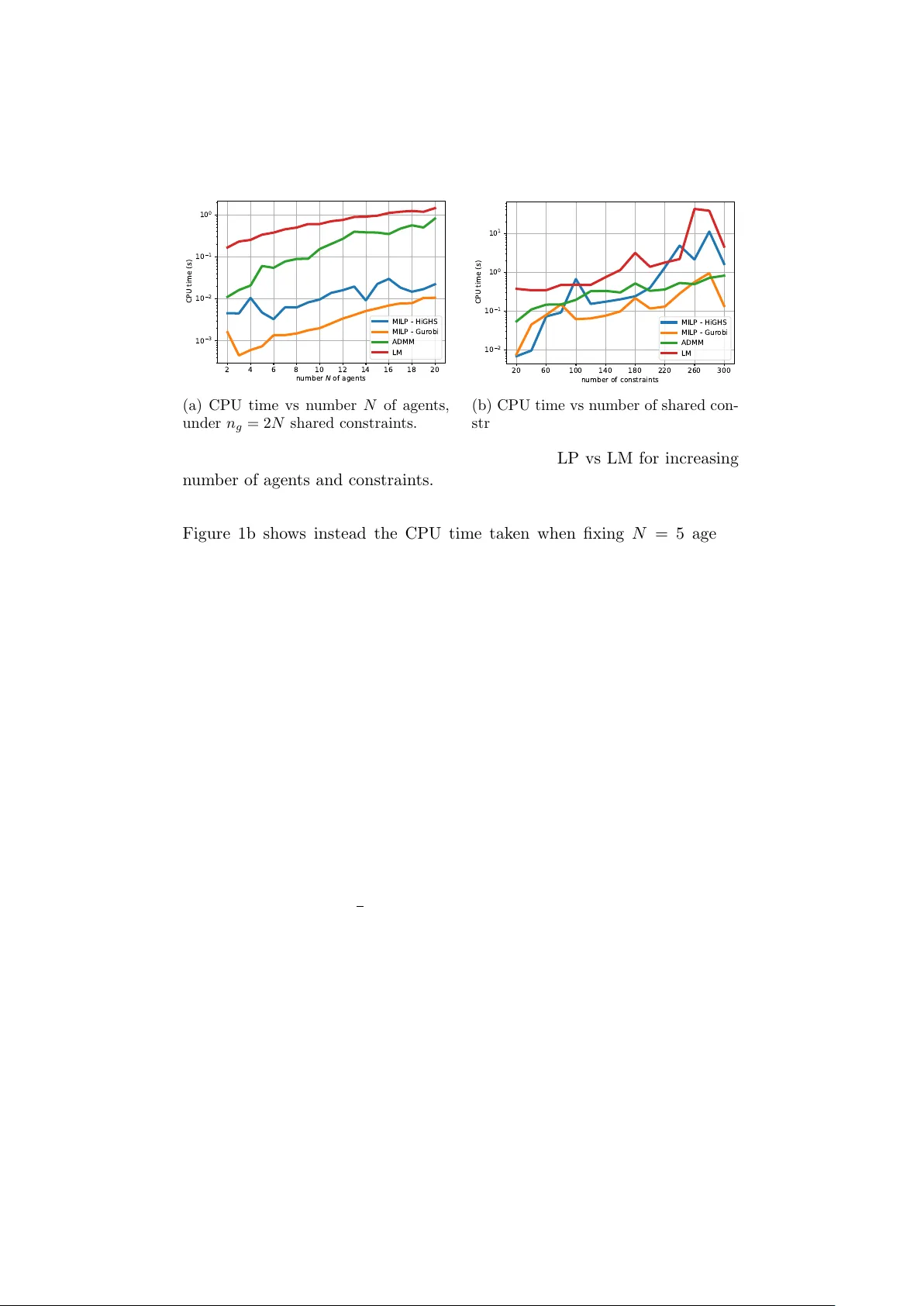
NashOpt - A Python Library for Computing Generalized Nash Equilibria Alb erto Bemp orad ∗ Marc h 19, 2026 Abstract NashOpt is an op en-source Python library for computing and de- signing generalized Nash equilibria (GNEs) in nonco operative games with shared constraints and real-v alued decision v ariables. The library exploits the join t Karush-Kuhn-T uc ker (KKT) conditions of all pla yers to handle b oth general nonlinear GNEs and linear–quadratic games, including their v ariational v ersions. Nonlinear games are solved via nonlinear least-squares formulations, relying on JAX for automatic differen tiation. Linear-quadratic GNEs are reformulated as mixed- in teger linear programs, enabling efficient computation of multiple equilibria. The framew ork also supp orts inv erse-game and Stack elb erg game-design problems. The capabilities of NashOpt are demonstrated through sev eral examples, including noncoop erativ e game-theoretic con- trol problems of linear quadratic regulation and mo del predictiv e con- trol. The library is a v ailable at https://github.com/bemporad/nashopt . 1 In tro duction Generalized games describ e situations where sev eral agents tak e decisions b y optimizing individual ob jective functions under lo cal and coupling con- strain ts on their decision v ariables. Examples include traffic participan ts us- ing the same roads, wireless systems sharing limited bandwidth, energy sys- tems where prosumers share transmission capacity and balance constraints [11, 40], or firms comp eting in a mark et [3]. The solution concept for these prob- lems, in whic h the cost function and the feasible set of each agen t dep ends ∗ The author is with the IMT Sc ho ol for Adv anced Studies, Piazza San F rancesco 19, Lucca, Italy . Email: alberto.bemporad@imtlucca.it . This work was funded by the Europ ean Union (ERC Adv anced Research Grant COMP A CT, No. 101141351). Views and opinions expressed are ho wev er those of the authors only and do not necessarily reflect those of the Europ ean Union or the Europ ean Research Council. Neither the Europ ean Union nor the gran ting authorit y can b e held responsible for them. on the decisions taken b y the other agen ts, is the generalized Nash equilib- rium (GNE), a state in which no agent has an incentiv e or the p ossibility to c hange their decision [2]. GNEPs hav e b een widely studied in the literature, with v arious algo- rithms prop osed for their solution, including splitting-based operator frame- w orks [41, 3], approaches built on augmented Lagrangian form ulations [36, 28, 9, 29], interior-point optimization strategies [13], Newton-t yp e algo- rithms [17], distributed algorithms [41, 39, 3], and learning-based meth- o ds only relying on measuring b est resp onses [15]. F or the sp ecific class of GNEPs in whic h the shared constrain ts are linear, efficien t solution metho ds exist for linear ob jectives [14, 21], multiparametric quadratic programming for strictly conv ex quadratic ob jectives [25], and distributed pay off-based algorithms for con v ex games [38]. 1.1 Con tribution Motiv ated by the relative scarcit y of softw are pack ages for solving rather general classes of GNEPs and their application to game-theoretic c on trol problems, in this paper w e describe the mathematical form ulations of our pac k age NashOpt , a Python library for solving GNEPs based on satisfying the KKT conditions of each play er join tly . The library supp orts nonlinear GNEPs, which are solved via nonlinear least-squares metho ds, and linear- quadratic GNEPs, whic h can b e solved more efficien tly via mixed-integer linear programming (MILP) and can b e used to enumerate multiple equi- libria for the same game corresp onding to different combinations of active constrain ts at optimality . W e also address game-design problems, where a cen tral authorit y can optimize some parameters of the game to ac hiev e a desired equilibrium in accordance with the optimistic Single-Leader-Multi- F ollo w er (SLMF) Stac kelberg game setting [1]. Moreo v er, w e lev erage the GNE solution metho ds to solv e game-theoretic c on trol problems, includ- ing non-coop erative linear quadratic regulation (LQR) and model predictiv e con trol (MPC) problems [24, 31]. The main purpose of the tool is to analyze and predict the effect of different agents pursuing their own ob jectives in a shared environmen t, and to design the game to promote desired equilibrium b eha viors. F or nonlinear GNEs, w e lev erage JAX [8] for automatic differen tiation and just-in-time compilation to achiev e high p erformance, and on the op en- source MILP solver HiGHS [27] or Gurobi [23] for the linear-quadratic case, using the so-called “big-M” form ulation to enco de the complemen tary slac k- ness conditions of the KKT system [26, 20]. The library is op en-source and can b e easily installed via pip install nashopt . W e refer the reader to the online do cumen tation at https:// github.com/bemporad/nashopt for a detailed description of the syntax and usage of the library . 2 1.2 Notation W e denote by R the set of real num b ers. Giv en N v ectors x i ∈ R n i , i = 1 , . . . , N , we denote b y x = col( x 1 , . . . , x N ) ∈ R n their vertical con- catenation, where n = P N i =1 n i . W e denote by 1 the vector of all ones of appropriate dimension, by I the identit y matrix, and b y e i the i th column of I . Given a matrix A , we denote b y A ⊤ its transpose and b y ∥ A ∥ F its F rob enius norm. 2 Problem F orm ulation Consider the follo wing game-design problem based on a multiparametric generalized Nash equilibrium problem (GNEP) with N play ers: min x ⋆ ,p ∈ P J ( x ⋆ , p ) s.t. x ⋆ i ∈ arg min x i f i ( x, p ) s.t. g ( x, p ) ≤ 0 h ( x, p ) = 0 ℓ i ≤ x ≤ u i x − i = x ⋆ − i i = 1 , . . . , N (1) where x i ∈ R n i collects the decision v ariables optimized by agen t i , i = 1 , . . . , N , x − i collects those of all other agents, x = col( x 1 , . . . , x N ) ∈ R n is the stack ed v ector of all agents’ decision v ariables, x ⋆ is constrained to b e a generalized Nash equilibrium (GNE) of the game corresponding to the parameter vector p ∈ R n p , n p ≥ 0, where by n p = 0 we mean that no parameter en ters (1). In (1), f i : R n → R is the ob jective of agent i , g : R n → R n g and h : R n → R n h define, resp ectively , shared inequality and equalit y constraints, and ℓ i ∈ ( R ∪ {−∞} ) n i , u i ∈ ( R ∪ { + ∞} ) n i define the (lo cal) b ox constraints for each play er i . Moreo ver, J : R n × R n p → R is the ob jectiv e function used to shap e the desired equilibrium of the game, and P ⊆ R n p is a giv en feasible set for the parameter v ector p , suc h as the h yp er- b o x P = { p ∈ R n p : ℓ p ≤ p ≤ u p } where ℓ p , u p are (p ossibly infinite) b ounds. Problem (1) is also referred to as an optimistic equilibrium of Single-Leader- Multi-F ollo w er (Stac k elb erg) game [1], with the leader optimizing p and the follo w ers pla ying the GNEP determined b y p . F or an y given p , a GNE x ⋆ is a vector for which no agent can reduce their cost giv en the strategies of the other pla y ers and feasibilit y constrain ts, i.e., f i (col( x ⋆ i , x ⋆ − i ) , p ) ≤ f i (col( x i , x ⋆ − i ) , p ) ∀ x i ∈ X i ( x ⋆ − i , p ) where, with a slight abuse of notation, we denoted by col( x i , x − i ) the v ector obtained by collecting the comp onen ts of x i and x − i in the right order, and 3 X i ( x ⋆ − i , p ) ⊆ R n i is the feasible set of play er i defined by the constraints in (1) giv en the strategies x − i of the other play ers. W e highlight special cases of (1) in the next sections. 2.1 Solving a sp ecific GNEP T o just solv e a given game, we set J ( x ⋆ , p ) ≡ 0 and P = { p 0 } a singleton, leading to the standard GNEP: x ⋆ i = arg min ℓ i ≤ x i ≤ u i f i ( x, p 0 ) s.t. g ( x, p 0 ) ≤ 0 , h ( x, p 0 ) = 0 x − i = x ⋆ − i , i = 1 , . . . , N . (2) 2.2 Finding a parameter v ector for which a GNE exists If no specific equilibrium is desired, we can set J ( x ⋆ , p ) ≡ 0 and let P b e a non-singleton set, leading to the problem of finding a parameter vector p ∈ P for which an equilibrium exists. 2.3 In v erse game problem Giv en an observ ed agents’ equilibrium x d es (or a desired one we wish to ac hiev e), b y setting J ( x ⋆ , p ) = ∥ x ⋆ − x des ∥ 2 2 (or J ( x ⋆ , p ) = ∥ x ⋆ − x des ∥ ∞ , ∥ x ⋆ − x des ∥ 1 ), we solve the inverse game of finding a vector p (if one exists) suc h that x ⋆ ≈ x d es . 3 KKT Conditions and Nonlinear Least-Squares F orm ulation Let us assume that f i , g , and h are con tin uously differen tiable with resp ect to x i and that suitable constraint qualifications hold, such as the Linear Indep endence Constraint Qualification (LICQ) condition at the GNE x ⋆ ( p ) 1 . Then, the necessary KKT conditions of optimality for each pla y er i read as 1 The LICQ condition is v erified if the gradien ts of the activ e constraints at x ⋆ ( p )  ∇ x i g j ( x ⋆ , p ) : j ∈ A ( x ⋆ )  ∪  ∇ x i h k ( x ⋆ , p )  ∪  ± e k : x ⋆ i,k = ℓ i,k or u i,k  are linearly indep endent, where e k is the k -th unit v ector of appropriate dimension, A ( x ⋆ ) = { j : g j ( x ⋆ , p ) = 0 } is the set of active inequality constraints at x ⋆ , and x i,k , ℓ i,k , and u i,k are the k -th comp onents of x i , ℓ i , and u i , respectively . 4 follo ws [34, Theorem 12.1]: ∇ x i f i ( x, p ) + ∇ x i g ( x, p ) ⊤ λ i + ∇ x i h ( x, p ) ⊤ µ i − v i + y i = 0 (3a) h ( x, p ) = 0 (3b) g ( x, p ) ≤ 0 , ℓ ≤ x ≤ u (3c) λ i ≥ 0 , v i ≥ 0 , y i ≥ 0 (3d) λ i,j g j ( x, p ) = 0 , v i,k ( x i,k − ℓ i,k ) = 0 , y i,k ( u i,k − x i,k ) = 0 (3e) j = 1 , . . . , n g , k = 1 , . . . , n i , i = 1 , . . . , N where λ i ∈ R m i denotes the vector of Lagrange multipliers of pla y er i asso- ciated with the shared inequalit y constraints g ( x, p ) ≤ 0, µ i the multipliers corresp onding to the shared equality constraints h ( x, p ) = 0, and v i , y i the m ultipliers asso ciated with bound constraints on x i . Note that the prob- lem setting in (1) could b e immediately extended to allo w for player-sp e cific constrain ts with coupling of the form g i ( x, p ) ≤ 0, h i ( x, p ) = 0 in the KKT system (3). A generalized Nash equilibrium is a p oin t x ⋆ for whic h the KKT sys- tem (3) holds for al l players simultane ously . The KKT conditions can be expressed as the follo wing zero-finding problem: 0 = ∇ x i f i ( x, p ) + ∇ x i g ( x, p ) ⊤ λ i + ∇ x i h ( x, p ) ⊤ µ i 0 = h ( x, p ) 0 = q λ 2 i,j + g j ( x, p ) 2 − λ i,j + g j ( x, p ) 0 = q v 2 i,k + ( ℓ i,k − x i,k ) 2 − v i,k + ℓ i,k − x i,k 0 = q y 2 i,k + ( x i,k − u i,k ) 2 − y i,k + x i,k − u i,k k = 1 , . . . , n i , i = 1 , . . . , N , j = 1 , . . . , n g (4) where the last three residuals enco de the primal feasibility (3c), dual feasi- bilit y (3d), and complementary slac kness conditions (3e) using the Fischer- Burmeister nonlinear complementarit y problem (NCP) function ϕ : R → R [19, 16] comp onen t wise ϕ ( α, β ) ≜ p α 2 + β 2 − α − β = 0 ⇐ ⇒ αβ = 0 , α ≥ 0 , β ≥ 0 . By letting z b e the vector collecting x , { λ i } , { µ i } , { v i } , and { y i } , we can express the join t KKT conditions as R ( z , p ) = 0 (5) where R ( z , p ) is the residual function defined in (4). In the sequel, we will denote by ν = col( λ, µ, v , y ) the stack ed vector of all dual v ariables, 5 so that z = col( x, ν ) is the o verall v ector of primal and dual v ariables. Giv en a solution z ⋆ ( p ) satisfying (5), we will implicitly denote by x ⋆ ( p ) the corresp onding GNE is obtained by extracting from z ⋆ ( p ) the comp onen ts corresp onding to the primal v ariables. W e will also denote by R ( z ) the residual function when p is om itted or fixed. F or conditions of existence of a GNE for a given p , such as nonemptiness and compactness of the set of feasible decision vectors, conv exity assump- tions on f , g , and linearity of h , and constraint qualifications, we refe r the reader to [18]. W e remark that only relying on the joint KKT conditions (3) to characterize GNEs would require additional regularit y assumptions. In NashOpt , these conditions are not v erified n umerically b y the soft ware. Con- sequen tly , when the assumptions ab ov e are violated, solving the KKT system should b e in terpreted as a heuristic computational approach for computing stationary points of the join t KKT system that, how ever, are not guaranteed a priori to be GNEs. On the other hand, in the case a zero residual R is ac hiev ed within a given tolerance at a certain x ⋆ , whether this corresp onds to a GNE or not can b e immediately chec ked a p osteriori by verifying that, for each play er i , the b est resp onses ¯ x i ( x ⋆ − i , p ) ≈ x ⋆ i , or that the asso ciated v alue function f i (col( ¯ x i , x ⋆ − i ) , p ) ≈ f i ( x ⋆ , p ). 3.1 Determining a GNE via nonlinear least-squares F or a giv en parameter p 0 , we can compute the corresponding z ⋆ ( p 0 ) by minimizing the squared residual z ⋆ ( p 0 ) ∈ arg min z 1 2 ∥ R ( z , p 0 ) ∥ 2 2 (6) that serv es as a merit function for the zero-finding problem (5) [16, 13]. The nonlinear least-squares problem (6) can b e solv ed via standard metho ds, suc h as Lev en b erg-Marquardt (LM) algorithms [30, 33], p ossibly exploiting sparsit y in the Jacobian of R ( z , p 0 ) with resp ect to z . If the minim um residual R ( z ⋆ ( p 0 ) , p 0 ) of the nonlinear least-squares problem (6) is zero (or, more realistically , b elo w a giv en p ositiv e tolerance), then z ⋆ ( p 0 ) con tains a GNE solution x ⋆ ( p 0 ) and the asso ciated Lagrange multipliers for each agen t’s problem asso ciated with the parameter v ector p 0 . 3.2 V ariational GNE V ariational GNEs (vGNEs) are obtained b y simply enforcing that the La- grange m ultipliers associated with the shared constraints are the same for all pla y ers, i.e., by replacing { λ i } with a single vector λ and { µ i } with a single v ector µ , which further reduces the num b er of v ariables in the zero-finding problem (5). 6 3.3 Game design T o solve the game-design problem (1), w e can em b ed the KKT conditions (3) in the optimization of p , leading to the following mathematical program with equilibrium constrain ts (MPEC) [32, 22]: min p,z J ([ I 0] z , p ) s.t. R ( z , p ) = 0 , p ∈ P . (7) Problem (7) can b e solved via constrained nonlinear programming metho ds with resp ect to b oth z and p . T o av oid the complexity of dealing with the equilibrium constrain ts, in our approach we solve the game-design problem (1) b y relaxing them and solving instead the follo wing nonlinear programming problem: min p,z J ([ I 0] z , p ) + ρ 2 ∥ R ( z , p ) ∥ 2 2 s.t. p ∈ P (8) where ρ > 0 is a p enalty parameter. By letting ρ → ∞ , the solution of (8) approac hes that of (7). When P is a h yp er-b o x (with p ossibly infinite lo wer and/or upp er b ounds on some parameters), Problem (8) can b e solved very efficien tly via b ound-constrained nonlinear optimization methods, such as L-BF GS-B [10]. The c hoice of the initial p oin t ( z , p ) and of the p enalt y ρ are crucial to ac hiev e conv ergence to a meaningful solution of (8); in particular, excessiv ely small v alues of ρ ma y lead to solutions that are far from satisfying the KKT conditions, while very large v alues of ρ ma y cause the n umerical solv er to ignore the game-design ob jectiv e J ( x, p ). In practice, we can solve (8) with a mo derate v alue of ρ to get a v alue ( ¯ z ⋆ , ¯ p ⋆ ) and then refine the GNE b y solving the nonlinear least-squares problem (6) with hot-start at ( ¯ z ⋆ , ¯ p ⋆ ). 3.4 Non-smo oth regularization When designing a parameter v ector p , or finding an equilibrium among man y existing ones for a giv en p 0 , w e can add the regularization term J reg ( x, p ) = α 1 ∥ x ∥ 1 + α 2 ∥ x ∥ 2 2 , α 1 , α 2 ≥ 0 in the game-design ob jective J ; for example, w e can promote sparsity of the GNE x ⋆ b y choosing a sufficiently large α 1 . When α 1 > 0, due to the non-differen tiabilit y of the ℓ 1 -norm at zero, we can reformulate the problem b y splitting x in to p ositiv e and negativ e parts, x = x p − x m , with x p , x m ≥ 0 and apply the result in [5, Corollary 1] to minimize min p,x p ,x m ,ν J ( x p − x m , p ) + ρ 2 ∥ R (col( x p − x m , ν ) , p ) ∥ 2 2 + α 1 1 ⊤ ( x p + x m ) + α 2 ( ∥ x p ∥ 2 2 + ∥ x m ∥ 2 2 ) s.t. p ∈ P , x p ≥ 0 , x m ≥ 0 (9) 7 where ν collects all dual v ariables. In the sp ecial case we are just lo oking for a sparse GNE with no game- design ob jective (i.e., J ( x, p ) ≡ 0) and α 2 > 0, by letting α 3 ≜ √ 2 α 2 , w e ha v e J reg ( x, p ) = α 1 1 ⊤ ( x p + x m ) + α 2 ( ∥ x p ∥ 2 2 + ∥ x m ∥ 2 2 ) = 1 2     α 3 x p + α 1 α 3 1     2 2 + 1 2     α 3 x m + α 1 α 3 1     2 2 + const. Then, w e can equiv alen tly solv e min p,x p ,x m ,ν 1 2             α 3 x p + α 1 α 3 1 α 3 x m + α 1 α 3 1 √ ρ R (col( x p − x m , ν ) , p )             2 2 s.t. p ∈ P , x p ≥ 0 , x m ≥ 0 . (10) When P is a hyper-b ox (with p ossibly infinite lo w er and/or upp er bounds on some parameters), or a singleton { p 0 } as a sp ecial case, Problem (9) can b e solv ed as a b ound-constrained nonlinear least-squares problem, suc h as via a trust-region reflective algorithm [12]. Low er and upp er b ounds ℓ ≤ x ≤ u can b e explicitly included in (9) and (10) by tightening the nonnegativity constrain ts on x p and x m , i.e., b y setting max { 0 , ℓ } ≤ x p ≤ max { 0 , u } , max { 0 , − u } ≤ x m ≤ max { 0 , − ℓ } . The approac h can b e immediately extended to the case J ( x, p ) = 1 2 ∥ f J ( x, p ) ∥ 2 2 for some vector function f J : R n × R n p → n f b y extending the residual v ector in (10) with f J ( x p − x m , p ). 4 Linear Quadratic Games Consider the follo wing sp ecial case of (1) where the agents’ cost functions are quadratic and the constrain ts are linear: min p,x ⋆ J ( x ⋆ , p ) s.t. x ⋆ i ∈ arg min x i f i ( x, p ) = 1 2 x ⊤ Q i x + ( c i + F i p ) ⊤ x s.t. Ax ≤ b + S p A eq x = b eq + S eq p ℓ i ≤ x ≤ u i x − i = x ⋆ − i i = 1 , . . . , N (11) 8 where x ⋆ is the generalized Nash equilibrium of the Linear-Quadratic (LQ) game with N play ers, ( Q i , c i , F i ) define the quadratic cost function for agen t i , with Q i = ( Q i ) ⊤ ∈ R n × n , and the diagonal blo ck Q i ii ⪰ 0, c i ∈ R n , F i ∈ R n × n p , matrices A ∈ R n g × n , b ∈ R n g , S ∈ R n g × n p define the shared linear inequality constraints, A eq ∈ R n h × n , b eq ∈ R n h , S eq ∈ R n h × n p define the shared linear equalit y constrain ts. W e consider as game-design function J ( x, p ), if any is given, the sum of con v ex piecewise affine functions J PW A ( x, p ) = n J X j =1 max k =1 ,...,n j D j k x + E j k p + h j k (12a) or the con v ex quadratic function J Q ( x, p ) = 1 2 [ x T p T ] Q J " x p # + c T J " x p # (12b) where Q J = Q ⊤ J ⪰ 0, Q J  = 0, Q J ∈ R ( n + n p ) × ( n + n p ) , c J ∈ R n + n p , or the sum of b oth, i.e., J ( x, p ) = J PW A ( x, p ) + J Q ( x, p ) . (12c) Sp ecial cases are: ( i ) J PW A ( x, p ) = J Q ( x, p ) ≡ 0 for no game design; ( ii ) J PW A ( x, p ) = ∥ x − x des ∥ ∞ (i.e., n J = 1, n 1 = 2 n , D 1 = [ I − I ] ⊤ , E 1 = 0, h 1 = col( − x des , x des )), or J PW A ( x, p ) = ∥ x − x des ∥ 1 (i.e., n J = n , n j = 2, D j, 1 = e ⊤ j , D j, 2 = − e ⊤ j , E j, 1 = E j, 2 = 0, h j, 1 = − x des , j , h j, 2 = x des , j ), or J Q ( x, p ) = 1 2 ∥ x − x des ∥ 2 2 for inv erse game problems; ( iii ) the so cial welfar e quadratic ob jectiv e J Q ( x, p ) = P N i =1 f i ( x, p ). F or conv enience, let us embed finite low er and upp er b ounds on x into the inequalit y constrain ts b y defining ¯ A =     A I u − I ℓ     , ¯ b =     b u u − ℓ ℓ     , ¯ S =     S 0 0     where I ℓ and I u collect the rows of the iden tit y matrix corresponding, resp ec- tiv ely , to finite upp er and low er b ound, and ℓ ℓ and u u are the corresp onding b ounds. Let m b e the total num b er of resulting inequality constraints. The KKT conditions for eac h pla y er’s optimization problem are neces- sary and sufficient for optimality , due to the conv exity of the cost functions and constraints, and can b e used to c haracterize the generalized Nash equi- 9 libria of the game: Q i i x + c i i + F i i p + ¯ A ⊤ i λ i + A ⊤ eq ,i µ i = 0 ¯ Ax ≤ ¯ b + ¯ S p A eq x = b eq + S eq p λ i ≥ 0 λ i,j ( ¯ A j x − ¯ b j − ¯ S j p ) = 0 , i = 1 , . . . , N (13) where Q i i collects the rows of Q i corresp onding to play er i ’s v ariables, ¯ A i collects the columns and rows of ¯ A where x i is inv olved, A eq ,i is defined sim- ilarly , and λ i , µ i , are the Lagrange m ultipliers asso ciated with the inequalit y and equality constraints, respec tiv ely , where the v ariables in x i app ear. Note that the LQ problem (11) could b e extended to handle play er-sp ecific linear constrain ts with coupling of the form A i x ≤ b i + S i p , A i eq x = b i eq + S i eq p , by c hanging (13) accordingly . By stacking the KKT conditions (13) for all pla yers, w e can rewrite the generalized Nash equilibrium conditions as a single mixed-in teger linear program (MILP) using standard big-M constrain ts to mo del the comple- men tarit y conditions (see, e.g., [26, Prop osition 2]): min p,x,λ,µ,δ,σ 1 2 [ x T p T ] Q J " x p # + c T J " x p # + n J X j =1 σ j s.t. σ j ≥ D j k x + E j k p + h j k , k = 1 , . . . , n j Q i i x + c i i + F i i p + ¯ A ⊤ i λ i + A ⊤ eq ,i µ i = 0 ¯ Ax ≤ ¯ b + ¯ S p A eq x = b eq + S eq p λ i ≥ 0 , i = 1 , . . . , N ¯ Ax − ¯ b − ¯ S p ≤ M (1 − δ ) λ i ≤ M δ, i = 1 , . . . , N δ ∈ { 0 , 1 } m (14) where M ∈ R is a sufficiently large p ositive constant, δ is a vector of binary v ariables in tro duced to mo del the complementarit y conditions, and σ is a v ector of auxiliary v ariables used to define an upp er-b ound the ob jective function, σ ∈ R n J . Clearly , at optimality P n J i =1 σ j = J PW A ( x, p ), as the first n j inequalities in (14) b ecome all active. Note that using the same vector δ for all pla yers ensures that shared constrain ts are activ e/inactiv e for all pla y ers sim ultaneously . Problem (14) can b e either solved with respect to p, x, λ, µ, δ, σ b y MILP when J Q ( x, p ) ≡ 0, or by mixed-integer quadratic programming (MIQP) otherwise. 10 4.1 Extracting m ultiple equilibria F or the same parameter vector p , multiple generalized Nash equilibria ma y exist that corresp ond to differen t com binations ¯ δ of activ e inequality con- strain ts, as recently explicitly characterized in [25]. T o extract multiple equilibria, we can iteratively solv e the MILP ab ov e after adding the follow- ing “no-go o d“ constraint X i : ¯ δ i =1 δ i − X i : ¯ δ i =0 δ i ≤ m X i =1 ¯ δ i ! − 1 (15) whic h preven ts the MILP from returning the same combination ¯ δ of activ e constrain ts in all subsequen t iterations. 4.2 V ariational GNE of LQ games As for the nonlinear case, a vGNE can b e obtained b y enforcing that the Lagrange m ultipliers asso ciated with the shared constrain ts are the same for all pla y ers, whic h further reduces the num b er of v ariables in (14). 4.2.1 Pro ximal ADMM solver F or vGNEs of LQ games with fixed parameter p = p 0 and no game ob jectiv e, w e also consider the pro ximal-ADMM algorithm in [7] as an alternative approac h to compute a vGNE. T o apply the metho d, that only handles equalit y constraints, we reformulate the problem as the following LQ game with N + 1 play ers: x ⋆ i ∈ arg min x i 1 2 x ′ Q i x + ( c i ) T x s.t. ¯ Ax + s ⋆ = ¯ b, A eq x = b eq x − i = x ⋆ − i , i = 1 , . . . , N s ⋆ ∈ arg min s 1 2   ¯ Ax ⋆ + s − ¯ b   2 2 s.t. ¯ Ax ⋆ + s = ¯ b, s ≥ 0 (16) where, without loss of generalit y , we hav e tak en p 0 = 0. The proximal- ADMM iterations for the reform ulation (16) are as follo ws: x k +1 i ∈ arg min x i 1 2 x ′ i Q i ii x i + ( c i i + Q i i, − i ¯ x k − i + ( λ k ) ⊤ ¯ A i + ( µ k ) ⊤ A eq ,i ) x i + γ 2 ∥ x i − x k i ∥ 2 2 + ρ 2 ( ∥ ¯ A i x k i + ¯ A − i ¯ x k − i + s k − ¯ b ∥ 2 2 + ∥ A eq ,i x i + A eq , − i ¯ x k − i − d ∥ 2 2 ) (17a) s k +1 ∈ arg min s ≥ 0 1 + ρ 2    ¯ Ax k +1 + s − ¯ b    2 2 + ( λ k ) ⊤ s + γ 2 ∥ s − s k ∥ 2 2 (17b) λ k +1 = λ k + ρ ( ¯ Ax k +1 + s k +1 − ¯ b ) (17c) µ k +1 = µ k + ρ ( A eq x k +1 − b eq ) (17d) 11 where ¯ x k − i collects the comp onen ts of x k +1 1 , . . . , x k +1 i − 1 , x k i +1 , . . . , x k N , γ > 0 is the pro ximal parameter, and ρ is the augmented Lagrangian parameter. The iterations (17) admit a closed-form solution: the x i -up date in (17a) is an unconstrained strongly conv ex quadratic program (QP) that can b e solv ed b y caching the Cholesky decomp ositions of Q i ii + γ I + ρ ( ¯ A ⊤ i ¯ A i + A ⊤ eq ,i A eq ,i ) for each pla y er i and then, at eac h iteration k , solving tw o triangular linear systems; the ev aluation of s k +1 also admits the closed-form solution s k +1 = 1 1 + ρ + γ max  (1 + ρ )( ¯ b − ¯ Ax k +1 ) + γ s k − µ k , 0  as, by completing the squares, (17b) is equiv alent to the pro jection of a v ector on to the nonnegativ e orthant. 5 Game-Theoretic Con trol 5.1 Game-theoretic linear quadratic regulation W e consider a non-co op erativ e multi-agen t linear-quadratic regulator (LQR) problem where N agents control a shared discrete-time linear dynamical system x ( t + 1) = Ax ( t ) + B u ( t ) , u ( t ) = col( u 1 ( t ) , . . . , u N ( t )) y ( t ) = C x ( t ) (18) where x ( t ) ∈ R n x is the state vector at step t = 0 , 1 , . . . , y ( t ) is the output v ector, and u ( t ) ∈ R n u is the input vector partitioned among the N agents, with u i ( t ) ∈ R n i b eing the input applied b y agent i at time t , and n u = P N i =1 n i . Each agen t applies their control input u i ( t ) according to the state- feedbac k la w u i ( t ) = − K i x ( t ) where K i ∈ R n i × n x is the LQR gain corresp onding to weigh t matrices Q i ∈ R n x × n x ⪰ 0, suc h as Q i = C ⊤ Q y i C with Q y i ⪰ 0, and R i ∈ R n i , R i ≻ 0. W e approximate the desired LQR gain K i as a function of the other agen ts’ gains K − i b y running the follo wing Riccati-based iterations K k i = ( R i + B T i X k i B i ) − 1 B T i X k i ( A − B − i K − i ) A k = A − B − i K − i − B i K k i X k +1 i = Q i + A T k X k i A k + ( K k i ) T R i K k i (19) from X 0 i = Q i for k = 1 , . . . , N LQR . Then, w e define eac h agen t’s cost function as the squared F rob enius norm of the deviation from its optimal gain K N LQR i ( K − i ): f i ( K i , K − i ) = 1 2 ∥ K N LQR i ( K − i ) − K i ∥ 2 F . 12 Let K = [ K ⊤ 1 · · · K ⊤ N ] ⊤ denote the stack ed feedback gain. A Nash equilib- rium is a feedbac k gain matrix K ⋆ suc h that K ⋆ i ∈ arg min K i f i ( K i , K ⋆ − i ) ∀ i = 1 , . . . , N . The equilibrium can b e computed as the solution of a Nash equilibrium problem by using the nonlinear least-squares approach (6) (without param- eter p 0 ), using the cen tralized LQR solution K LQR asso ciated with ( A, B , P i Q i , blkdiag( R 1 , . . . , R N )) as initial guess. Note that, in this case, the op- timalit y conditions (4) reduce to ∇ K i f i ( K i , K − i ) = K N LQR i ( K − i ) − K i = 0 for all i = 1 , . . . , N , where with a slight abuse of notation, we considered K i as its v ectorized version; hence, the nonlinear least-squares problem (6) reduces to minimizing the sum of the squared deviations from the optimal gains, i.e., P N i =1 ∥ K N LQR i ( K − i ) − K i ∥ 2 F . Alternativ ely , the coupled discrete-time algebraic Riccati equations can b e solved using Riccati-based iterations as describ ed in [35, Section I I I.B] un til con v ergence is reached within a giv en tolerance. 5.2 Game-theoretic model predictiv e con trol Consider again the discrete-time linear system (18) with N agents com- p eting to mak e the output y ( t ) trac k a given set-p oint r ( t ) ∈ R n y . By letting ∆ u ( t ) = u ( t ) − u ( t − 1) denote the input increment at time t , eac h agen t i c ho oses the sequence ∆ u i ≜ { ∆ u i,k } T − 1 k =0 of input incremen ts o v er a prediction horizon of T b y solving the following standard discrete-time finite-horizon linear optimal con trol problem [6, 4]: (∆ u i , ϵ i ) ∈ arg min T − 1 X k =0 ( y k +1 − r ( t )) ⊤ Q y ,i ( y k +1 − r ( t )) + ∆ u ⊤ i,k Q ∆ u,i ∆ u i,k ! + q ϵ,i ϵ i s.t. x k +1 = Ax k + B u k y k +1 = C x k +1 u k,i = u k − 1 ,i + ∆ u k,i u − 1 = u ( t − 1) ∆ u min ≤ ∆ u k ≤ ∆ u max u min ≤ u k ≤ u max y min − P N i =1 ϵ i ≤ y k +1 ≤ y max + P N i =1 ϵ i ϵ i ≥ 0 i = 1 , . . . , N , k = 0 , . . . , T − 1 . (20) In (20), Q ∆ u,i ≻ 0 and Q y ,i ⪰ 0; for example, if an agen t is interested in con trolling only a subset I i of the components of the output v ector with unit w eigh ts, w e ha v e Q y ,i = P j ∈ I i e j e ⊤ j . The slac k v ariables ϵ i ≥ 0 are used to soften the shared output constrain ts (with linear p enalt y q ϵ,i ≥ 0). The predicted tra jectories { x k , y k , u k } in (20) satisfy the dynamic equa- tions (18) ov er the prediction horizon k = 0 , . . . , T , with initial condition 13 x 0 = x ( t ) and u − 1 = u ( t − 1). Note that eac h agent optimizes the sequence of input incremen ts ∆ u i and the slac k v ariable ϵ i , so that constraints on inputs, input incremen ts, and slacks are local to each agent, while output constrain ts are shared among all agents, each one softening them with p os- sibly different slacks ϵ i . Hence, the resulting game-theoretic MPC problem is the GNE problem of finding sequences { ∆ u ⋆ i } N i =1 (and slacks { ϵ ⋆ i } N i =1 ) optimizing (20) for all agen ts i = 1 , . . . , N sim ultaneously . In a receding- horizon fashion, only the first inputs u i ( t ) = u i ( t − 1) + ∆ u ⋆ i, 0 are applied for i = 1 , . . . , N , and the en tire pro cedure is rep eated at t + 1. The n um b er of constraints in each agen t’s problem (20) can b e reduced b y imp osing the constraints only on a shorter constraint horizon of T c < T steps. This can b e especially useful when T is large but w e wan t to limit the num b er of Lagrange multipliers and binary v ariables inv olved in the MILP reformulation (14) of the GNEP , in whic h w e remov e p , σ , and the ob jectiv e function (12a), as w e are only interested in computing the GNE of the nonco op erativ e MPC problem. If a variational equilibrium is requested, the additional equalities enforc- ing common Lagrange multipliers for the shared output constraints in (20) can be imp osed. In Section 6.5, we will consider an example of nonco op- erativ e MPC and show that it can deviate significantly from the c o op er a- tive and c entr alize d MPC solution in which all mov es are optimized join tly b y solving a quadratic programming (QP) problem with decision v ariables ∆ u = col(∆ u 1 , . . . , ∆ u N ), ϵ = col( ϵ 1 , . . . , ϵ N ) and cost function giv en by the sum of all agen ts’ costs in (20). 6 Examples W e rep ort several numerical tests to illustrate the metho ds describ ed in the previous sections for computing and designing generalized Nash equilibria. All tests are run on a Macb o ok Pro with Apple M4 Max chip and 64 GB RAM using JAX [8] for automatic differentiation and just-in-time compila- tion of the in v olv ed functions when required. 6.1 Linear-quadratic game Let us first consider a simple linear-quadratic game with N = 3 agents, eac h con trolling t w o decision v ariables x i ∈ R 2 , i = 1 , 2 , 3, with cost functions f i ( x ) = 1 2 x ⊤ x + i 1 ⊤ x (21) 14 where x = col( x 1 , x 2 , x 3 ) ∈ R 6 , and shared constrain ts        − 0 . 4 − 0 . 1 − 2 . 1 1 . 6 − 1 . 8 − 0 . 8 0 . 5 − 1 . 2 − 1 . 1 − 0 . 9 0 . 6 2 . 3 0 − 1 . 1 0 . 5 − 0 . 6 0 . 0 1 . 2 − 0 . 7 0 − 0 . 9 − 0 . 2 0 . 3 − 1        x ≤        1 1 1 1        . The GNE is computed b y solving the MILP (14) with no parameter p , and optimal combinations extracted by iteratively adding the no-go o d con- strain t (15), leading to the three equilibrium solutions: x ⋆ 1 = [11 . 0588 2 . 7647 − 1 − 1 − 2 − 2] ⊤ x ⋆ 2 = [0 0 − 0 . 3436 − 1 . 5001 − 1 . 1599 − 0 . 7387] ⊤ x ⋆ 3 = [0 0 − 0 . 7966 − 0 . 8336 − 0 . 2783 − 0 . 1998] ⊤ . These corresp ond to the optimal active constraint com binations (1), (1 , 4), and (1 , 2 , 4), resp ectiv ely . By imp osing the additional constrain t that the Lagrange m ultipliers asso ciated with the shared constrain ts are the same for all agen ts, w e get the vGNE x ⋆ v = [0 . 3553 0 . 037 0 . 0431 − 1 . 5324 − 1 . 4232 − 1 . 408] ⊤ corresp onding to the activ e constrain t combination (1 , 4). The CPU time for computing eac h equilibrium ranges b etw een 4 . 7 and 10 . 1 ms for the non-v ariational case and is 8 . 3 ms for the v ariational one using the HiGHS solv er [27]. Note that infinitely many differen t GNEs ma y exist for the same com bination of activ e constrain ts, as clearly shown in [25]. F or comparison, w e also use the nonlinear least-squares approach (6) and compute the same vGNE x ⋆ v as ab o ve in 229 . 9 ms (10 LM iterations) starting from the initial guess x 0 = 0. The same vGNE is found again by running the pro ximal ADMM approach described in Section 4.2.1, where w e set γ = 1, ρ = 1, x 0 = 0, λ 0 = 0, which takes 13 . 9 ms (229 ADMM iterations). Next, w e further compare the MILP, LM, and proximal ADMM ap- proac hes on random GNE problems of increasing size. W e consider linear- quadratic games with N agen ts, each controlling n i = 2 decision v ariables, with cost functions f as in (21) and shared constraints defined by n g = 2 N random linear inequalities with unit right-hand side. The results are shown in Figure 1a, where, for an increasing n umber N of agen ts, w e report the CPU time for computing a GNE via MILP and for computing a vGNE b y LM and proximal ADMM. Computing GNEs on LQ games via MILP with HiGHS is ab out tw o orders of magnitude more efficient than b y LM, and ev en more by using Gurobi’s state-of-the-art MILP solver; it also out- p erforms proximal ADMM (which takes b etw een 258 and 1794 iterations). 15 2 4 6 8 10 12 14 16 18 20 n u m b e r N o f a g e n t s 1 0 3 1 0 2 1 0 1 1 0 0 CPU time (s) MILP - HiGHS MILP - Gur obi ADMM LM (a) CPU time vs num b er N of agents, under n g = 2 N shared constraints. 20 60 100 140 180 220 260 300 number of constraints 1 0 2 1 0 1 1 0 0 1 0 1 CPU time (s) MILP - HiGHS MILP - Gur obi ADMM LM (b) CPU time vs num b er of shared con- strain ts, with N = 5 agents. Figure 1: CPU time for computing a GNE via MILP vs LM for increasing n um b er of agen ts and constrain ts. Figure 1b shows instead the CPU time taken when fixing N = 5 agents and increasing the num b er of shared constraints n g up to 300, showing that MILP metho ds degrade more in p erformance compared to pro ximal ADMM due to the increasing n um b er of binary v ariables in (14). 6.2 In v erse linear-quadratic game design W e consider an inv erse game-design problem for a GNEP with N = 10 agen ts, each optimizing a vector x i ∈ R n i of n i = 10 v ariables ( x ∈ R 100 ), parameterized by a v ector p ∈ R n p , with n p = 5, with ∥ p ∥ ∞ ≤ 100. F or eac h giv en p , eac h agent i = 1 , . . . , N solves the con vex quadratic optimization problem defined in (11) with b ∈ R 50 , b eq ∈ R 5 . All matrices and vectors are randomly generated with appropriate dimensions, with Q i ≻ 0, and the b o x constrain ts are defined b y u = − ℓ = 10 · 1 . T o formulate the inv erse game problem in an ideal setting, we first com- pute a reference equilibrium x des and a corresp onding parameter vector ˆ p b y solving (11) with zero ob jective J ( x ⋆ , p ) = 0. Then, we solv e the inv erse game-design problem (14) by using either J ( x ⋆ , p ) = ∥ x ⋆ − x des ∥ ∞ (MILP problem) or J ( x ⋆ , p ) = 1 2 ∥ x ⋆ − x des ∥ 2 2 (MIQP problem) to retriev e a param- eter v ector p ⋆ that yields an equilibrium x ⋆ ( p ⋆ ) ≈ x des . W e use Gurobi’s solv ers in b oth cases. The parameter v ector p ⋆ is retrieved, resp ectively , in 0 . 0394 s by MILP with ∥ x ⋆ ( p ⋆ ) − x des ∥ ∞ = 5 . 4712 · 10 − 13 , and 0 . 0660 s by MIQP with ∥ x ⋆ ( p ⋆ ) − x des ∥ 2 = 1 . 2434 · 10 − 14 . 6.3 Stac k elb erg game Consider a problem with N agents (the follow ers), eac h controlling a decision v ariable x i ≥ 0, i = 1 , . . . , N , sub ject to the shared constraint P N i =1 x i ≤ C . 16 Eac h agen t i minimizes: f i ( x, p ) = a i x 2 i + N X j =1 Γ ij x i x j + π i ( x, p ) x i where a i > 0 is a self-cost co efficien t, Γ ∈ R N × N is a symmetric interaction matrix, and π i ( x, p ) is the nonlinear price function π i ( x, p ) = p 1 ,i + p 2   N X j =1 x j   2 . Here p = col( p 1 , 1 , . . . , p 1 ,N , p 2 ) is the vector of game parameters c hosen by the leader to minimize the loss function J ( x, p ) = N X i =1 x − D ! 2 + η N X i =1 ( p 1 ,i − ¯ p 1 ,i ) 2 − ρ N X i =1 π i ( x, p ) x i with p 1 ,i ∈ [ p 1 , min , p 1 , max ] and p 2 ∈ [ p 2 , min , p 2 , max ]. The numerical v alues are set as follows: N = 8, C = 1, D = 0 . 9, p 1 , min = − 5, p 1 , max = 0, p 2 , min = 0, p 2 , max = 0 . 2, ¯ p 1 ,i = − 2, η = 0 . 1, ρ = 0 . 3, and Γ =                  0 0 . 2 0 0 0 . 1 0 0 0 0 . 2 0 0 . 1 0 0 0 0 0 0 0 . 1 0 0 . 15 0 0 0 0 0 0 0 . 15 0 0 . 1 0 0 0 0 . 1 0 0 0 . 1 0 0 . 2 0 0 0 0 0 0 0 . 2 0 0 . 1 0 0 0 0 0 0 0 . 1 0 0 . 2 0 0 0 0 0 0 0 . 2 0                  , a =                  1 . 0 1 . 5 0 . 8 1 . 2 2 . 0 0 . 9 1 . 8 1 . 1                  . By setting ρ = 10 8 , (8) is solv ed with 83 LM iterations in 1.057 s starting from the initial guess p (0) 1 = p 1 , min + p 1 , max 2 , p (0) 2 = p 2 , min + p 2 , max 2 , and x (0) i = C N . The optimal parameters and related GNE are p ⋆ 1 = − [1 . 6174 1 . 8083 1 . 553 1 . 6970 1 . 9523 1 . 5737 1 . 9009 1 . 6576] ⊤ p ⋆ 2 = 0 . 1990 x ⋆ ( p ⋆ ) = [0 . 0882 0 . 1745 0 . 0413 0 . 1325 0 . 2002 0 . 0565 0 . 1945 0 . 1124] ⊤ where P N i =1 x ⋆ i ( p ⋆ ) ≈ 1 = C . The optimal v alue of the leader’s loss function is J ( x ⋆ ( p ⋆ ) , p ⋆ ) = 0 . 5637. W e observed that different initializations lead to differen t GNEs with differen t v alues of the leader’s loss function, due to the noncon v exit y of the optimization problem (8). 17 0 5 10 15 20 time step t − 5 . 0 − 2 . 5 0 . 0 2 . 5 5 . 0 game-theoretic LQR 0 5 10 15 20 time step t − 5 . 0 − 2 . 5 0 . 0 2 . 5 5 . 0 cen tralized LQR Figure 2: Game-theoretic vs centralized LQR 6.4 LQR game W e consider a linear system as in (18) with n x = 10 states and n u = 10 inputs, each one controlled by a different agent ( n i = 1 for all i = 1 , . . . , N , N = 10 agent s), with A, B ∈ R 10 × 10 randomly generated and scaled so that A is unstable with sp ectral radius equal to 1.1. W e consider state-weigh ting matrices Q i = e i e T i and R i = 10 for all i = 1 , . . . , N . In (19), w e set N L QR = 50, whic h is a long-enough horizon used to appro ximate the infinite-horizon cost, therefore pro viding a go o d appro xi- mation of the solution of the algebraic Riccati equation asso ciated with the quadruple (( A − B − i K − i ) , B i , Q i , R i ) for eac h agen t i . The problem is solved as in (6) (without parameter p 0 ) in 6.05 s (6 LM iterations), leading to an asymptotically closed-lo op matrix A − B K ⋆ with sp ectral radius 0.7525. F or comparison, the cen tralized (co op erativ e) LQR solution leads to a sp ectral radius of 0.3965. Solving the same problem by using the Riccati-based iterations described in [35, Section II I.B] leads to the same solution in 0.11 s (7 Riccati iterations). Figure 2 compares the closed-lo op step resp onses of the com bined output v ector y ( t ) = 1 ⊤ x ( t ) from v arious initial conditions x (0) for the nonco op er- ativ e LQR gain K ⋆ and the cen tralized LQR gain K LQR . 6.5 Game-theoretic MPC W e consider a linear system as in (18) with n x = 6 states, n u = 3 inputs, and n y = 3 outputs, eac h one controlled by a differen t agent ( n i = 1 for all i = 1 , 2 , 3, N = 3 agen ts), with A, B ∈ R 6 × 3 randomly generated and scaled so that A is stable with spectral radius equal to 0.95. The output matrix C ∈ R 3 × 6 is scaled so that the steady-state gain from inputs to outputs is the iden tit y matrix. Each agent i has state-w eighting matrix Q i = C ⊤ Q y ,i C , with Q y ,i = e i e ⊤ i , Q y ,i ∈ R 3 × 3 , and input-incremen t weigh ting Q ∆ u,i = 0 . 5 for i = 1 , 2 , 3. The prediction horizon is T = 10 and the constraint horizon 18 0 10 20 30 40 0 1 2 3 game-theoretic MPC y 1 y 2 y 3 0 10 20 30 40 time step t 0 1 2 3 4 u 1 u 2 u 3 (a) Game-theoretic MPC 0 10 20 30 40 0 1 2 3 centralized MPC y 1 y 2 y 3 0 10 20 30 40 time step t 0 1 2 3 4 u 1 u 2 u 3 (b) Centralized MPC Figure 3: Closed-loop tra jectories for linear MPC: comparison b etw een game-theoretic (comp etitiv e) and cen tralized (co op erativ e) form ulations. is T c = 3. F or all i = 1 , 2 , 3, the input constrain ts are 0 ≤ u i ≤ 4 and the output constrain ts are 0 ≤ y i ≤ 5, with slack p enalty q ϵ,i = 10 3 . The nonco op erativ e MPC problem is solv ed at each time step t = 0 , . . . , T sim − 1, with T sim = 40, by solving the MILP reformulation (14) of the GNEP (without parameter p and ob jectiv e function (12)) using the HiGHS solver [27]. The resulting closed-lo op tra jectories are sho wn in Figure 3a. F or compari- son, w e also sho w the closed-lo op tra jectories obtained b y solving a co op era- tiv e and cen tralized MPC problem at eac h time step t b y join tly optimizing all agen ts’ mo v es via the QP solver osQP [37]. The CPU time for solving eac h GNEP ranges b et w een 4 . 36 and 65 . 62 ms (HiGHS MILP), while the CPU time for solving eac h cen tralized MPC prob- lem ranges b et w een 0 . 57 and 2 . 80 ms (QP). 6.6 Computing sparse equilibria Consider a Nash equilibrium problem with N = 40 agents, eac h one con trol- ling a scalar decision v ariable x i and no free parameter (e.g., p = 0). The agen ts are grouped in to pairs (2 k − 1 , 2 k ), k = 1 , . . . , 20, with the agents’ ob jectiv es defined as f i ( x ) =  x 2 k − 1 − x 2 k  2 , k = ⌊ ( i + 1) / 2 ⌋ . Clearly , if for ev ery agent-pair k the corresponding v ariables x 2 k − 1 = x 2 k , w e ha v e a Nash equilibrium x ⋆ ∈ R N . Among the infinitely many Nash 19 0 1 2 3 4 5 α 1 0 10 20 30 40 n umber of nonzeros 0 20 40 60 optimal cost Figure 4: Num b er of nonzeros in x ⋆ and optimal cost J ( x ⋆ , 0) as a function of the ℓ 1 -regularization parameter α 1 . equilibria, w e w an t to minimize the game-design ob jectiv e J ( x, 0) = N X i =1 ( x i − x ref i ) 2 + α 1 ∥ x ∥ 1 where the comp onents of the reference vector x ref i = ⌈ ( i +1) / 2 ⌉ 10 , i = 1 , . . . , N , and α 1 > 0 promotes sparsity in the equilibrium solution. Figure 4 sho ws the num b er of nonzeros in the computed Nash equilib- rium x ⋆ and the optimal cost J ( x ⋆ , 0) as a function of the ℓ 1 -regularization parameter α 1 , obtained by solving Problem (10) with ρ = 10 4 and P = { 0 } . The CPU time is 1.4350 s on the first run due to JAX compilation time, and 29.9 ms on a v erage on the subsequent runs. As exp ected, as α 1 increases, the num b er of zeros in x ⋆ increases, leading to sparser Nash equilibria, at the expense of a larger optimal cost J ( x ⋆ , 0). Clearly , due to the equilibrium condition x ⋆ 2 k − 1 = x ⋆ 2 k , the num b er of nonzeros in x ⋆ can only decrease by t w o at a time as α 1 increases. Figure 5 shows the CPU time required to compute the sparse solution as a function of the num b er N of agents for α 1 = 2 using L-BFGS-B. The CPU time gro ws roughly linearly with N . Ac kno wledgmen ts W e thank the anonymous reviewers for their constructive comments and suggestions. 7 Conclusions In this pap er, w e hav e prop osed differen t simple metho ds for designing and computing generalized Nash equilibria in nonco op erative games with lo- 20 0 100 200 300 400 N 0 1 2 3 4 5 CPU time (s) Figure 5: CPU time to compute the Nash equilibrium as a function of the n um b er N of agents. cal and shared constraints. W e ha ve presented a mixed-integer linear or quadratic programming reformulation for computing all generalized Nash equilibria of a linear-quadratic game, as well as a nonlinear least-squares approac h for computing ge neralized Nash equilibria of a rather general class of nonlinear games. W e ha ve illustrated the prop osed metho ds on several n umerical examples, including linear-quadratic games, game-theoretic LQR and MPC con trol, inv erse games, and sparsity-promoting GNE computa- tions. W e believe that the prop osed methods and the associated open-source library can b e a useful to ol for researchers and practitioners working in the field of game-theory and game-theoretic control and its applications to en- gineering and economic systems. References [1] D. Aussel and A. Sv ensson. A short state of the art on m ulti-leader- follo w er games. In S. Demp e and J. Zemk oho, editors, Bilevel Opti- mization , v olume 161, pages 53–76. Springer, 2020. [2] D. Bauso. Game The ory with Engine ering Applic ations . SIAM, 2016. [3] G. Belgioioso, P . Yi, S. Grammatico, and L. P a v el. Distributed gen- eralized Nash equilibrium seeking: An operator-theoretic persp ective. IEEE Contr ol Systems Magazine , 42(4):87–102, August 2022. [4] A. Bemp orad. Hybrid T o olb ox – User’s Guide . Jan uary 2004. http: //cse.lab.imtlucca.it/ ~ bemporad/hybrid/toolbox . [5] A. Bemp orad. An L-BFGS-B approach for linear and nonlinear system iden tification under ℓ 1 and group-lasso regularization. IEEE T r ansac- 21 tions on A utomatic Contr ol , 70(7):4857–4864, 2025. code av ailable at https://github.com/bemporad/jax- sysid . [6] A. Bemp orad, M. Morari, and N.L. Rick er. Mo del Pr e dictive Contr ol T o olb ox for MA TLAB – User’s Guide . The Math works, Inc., 2004. http://www.mathworks.com/access/helpdesk/help/toolbox/mpc/ . [7] E. B¨ orgens and C. Kanzo w. ADMM-t yp e methods for generalized Nash equilibrium problems in Hilb ert spaces. SIAM Journal on Optimization , 31(1):377–403, 2021. [8] J. Bradbury , R. F rostig, P . Hawkins, M.J. Johnson, C. Leary , D. Maclaurin, G. Necula, A. Paszk e, J. V anderPlas, S. W anderman- Milne, and Q. Zhang. JAX: comp osable transformations of Python+NumPy programs, 2018. [9] L.F. Bueno, G. Haeser, and F.N. Ro jas. Optimalit y conditions and constrain t qualifications for generalized Nash equilibrium problems and their practical implications. SIAM Journal on Optimization , 29(1):31– 54, 2019. [10] R.H. Byrd, P . Lu, J. No cedal, and C. Zhu. A limited memory algo- rithm for b ound constrained optimization. SIAM Journal on Scientific Computing , 16(5):1190–1208, 1995. [11] H. Le Cadre, P . Jacquot ab d C. W an, and C. Alasseur. P eer-to-p eer electricit y mark et analysis: F rom v ariational to generalized Nash equi- librium. Eur op e an Journal of Op er ational R ese ar ch , 282:753–771, 2020. [12] T.F. Coleman and Y. Li. An interior trust region approach for nonlin- ear minimization sub ject to b ounds. SIAM Journal on Optimization , 6(2):418–445, 1996. [13] A. Drev es, F. F acc hinei, C. Kanzow, and S. Sagratella. On the solution of the KKT conditions of generalized Nash equilibrium problems. SIAM Journal on Optimization , 21(3):1082–1108, 2011. [14] A. Drev es and N. Sudermann-Merx. Solving linear generalized Nash equilibrium problems n umerically . Optimization Metho ds and Softwar e , 31(5):1036–1063, 2016. [15] F. F abiani and A. Bemp orad. An activ e learning metho d for solving comp etitiv e multi-agen t decision-making and control problems. IEEE T r ansactions on Automatic Contr ol , 70(4):2374–2389, 2025. co de av ail- ble at https://github.com/bemporad/gnep- learn . [16] F. F acchinei, A. Fischer, and C. Kanzo w. Regularity prop erties of a semismo oth reformulation of v ariational inequalities. SIAM Journal on Optimization , 8(3):850–869, 1998. 22 [17] F. F acchinei, A. Fisc her, and V. Piccialli. Generalized Nash equilibrium problems and Newton metho ds. Mathematic al Pr o gr amming , 117(1- 2):163–194, July 2007. [18] F. F acc hinei and C. Kanzow. Generalized Nash equilibrium problems. A nnals of Op er ations R ese ar ch , 175:177–211, 2010. [19] A. Fisc her. A sp ecial Newton-type optimization metho d. Optimization , 24(3–4):269–284, 1992. [20] B. F ranci, F. F abiani, M. Sc hmidt, and M. Staudigl. A Gauss–Seidel metho d for solving multi-leader-m ulti-follow er games. In Eur op e an Con- tr ol Confer enc e , pages 2775–2780, 2025. [21] G. Graser, T. Kreimeier, and A. W alther. Solving linear generalized Nash games using an active signature metho d. Optimization Metho ds and Softwar e , pages 1–24, 2025. [22] L. Guo, G.-H. Lin, and J.J. Y e. Solving mathematical programs with equilibrium constraints. Journal of Optimization The ory and Applic a- tions , 166:234–256, 2015. [23] Gurobi Optimization, LLC. Gurobi Optimizer Reference Man ual, 2024. [24] S. Hall, G. Belgioioso, D. Liao-McPherson, and F. D¨ orfler. Reced- ing horizon games with coupling constrain ts for demand-side manage- men t. In Pr o c. IEEE 61st Confer enc e on De cision and Contr ol , page 3795–3800, Decem b er 2022. [25] S. Hall and M. Bemp orad. Solving multiparametric generalized Nash equilibrium problems and explicit game-theoretic model predictive con- trol. 2025. a v ailable on arXiv at . Co de av ailable at https://github.com/bemporad/nash_mpqp . [26] W.P .M.H. Heemels, B. De Sch utter, and A. Bemp orad. Equiv alence of h ybrid dynamical mo dels. Automatic a , 37(7):1085–1091, July 2001. [27] Q. Huangfu and J.A.J. Hall. P arallelizing the dual revised sim- plex method. Mathematic al Pr o gr amming Computation , 10(1):119–142, 2018. [28] C. Kanzo w and D. Steck. Augmented Lagrangian metho ds for the solution of generalized Nash equilibrium problems. SIAM Journal on Optimization , 26(4):2034–2058, 2016. [29] S. Le Cleac’h, M. Sc hw ager, and Z. Manchester. ALGAMES: a fast aug- men ted Lagrangian solv er for constrained dynamic games. Autonomous R ob ots , 46(1):201–215, 2022. 23 [30] K. Lev enberg. A metho d for the solution of certain non-linear problems in least squares. Quarterly of Applie d Mathematics , 2(2):164–168, 1944. [31] M. Liu and I.V. Kolmanovsky . Input-to-state stability of Newton meth- o ds in Nash equilibrium problems with applications to game-theoretic mo del predictive control. arXiv pr eprint arXiv:2412.06186 , 2024. [32] Z.-Q. Luo, J.-S. Pang, and D. Ralph. Mathematic al pr o gr ams with e quilibrium c onstr aints . Cambridge Universit y Press, 1996. [33] D.W. Marquardt. An algorithm for least-squares estimation of non- linear parameters. Journal of the So ciety for Industrial and Applie d Mathematics , 11(2):431–441, 1963. [34] J. No cedal and S.J. W right. Numeric al Optimization . Springer, 2 edi- tion, 2006. [35] B. Nortmann, A. Monti, M. Sassano, and T. Mylv aganam. Nash equi- libria for linear quadratic discrete-time dynamic games via iterativ e and data-driven algorithms. IEEE T r ansactions on A utomatic Contr ol , 69(10):6561–6575, 2024. [36] J.-P . P ang and M. F ukushima. Quasi-v ariational inequalities, general- ized Nash equilibria, and m ulti-leader-follow er games. Computational Management Scienc e , 2(1):21–56, January 2005. [37] B. Stellato, G. Banjac, P . Goulart, A. Bemp orad, and S. Boyd. OSQP: An operator splitting solv er for quadratic programs. Mathematic al Pr o- gr amming Computation , 12:637–672, 2020. [38] T. T atarenko and M. Kamgarp our. Learning generalized Nash equi- libria in a class of conv ex games. IEEE T r ansactions on Automatic Contr ol , 64(4):1426–1439, 2018. [39] T. T atarenko, W. Shi, and A. Nedi ´ c. Geometric conv ergence of gra- dien t play algorithms for distributed Nash equilibrium seeking. IEEE T r ansactions on Automatic Contr ol , 66(11):5342–5353, 2021. [40] Z. W ang, F. Liu, Z. Ma, Y. Chen, W. W ei, and Q. W u. Dis- tributed generalized Nash equilibrium seeking for energy sharing games in prosumers. IEEE T r ansactions on Power Systems , 36(6):3973–3986, Septem b er 2021. [41] P . Yi and L. Pa vel. An op erator splitting approach for distributed gen- eralized Nash equilibria computation. Automatic a , 102:111–121, 2019. 24