A Structured Nonparametric Framework for Nonlinear Accelerated Failure Time Models (KAN-AFT)

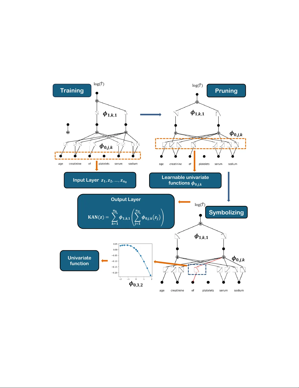
A Structured Nonparametric F ramew ork for Nonlinear Accelerated F ailure Time Mo dels (KAN-AFT) Mebin Jose 1 Jisha F rancis 1 ∗ Sudheesh Kumar Kattumannil 2 † 1 Departmen t of Mathematics, School of Adv anced Sciences, V ellore Institute of T ec hnology , V ellore, India, 632014 2 Applied Statistics Unit, Indian Statistical Institute, Chennai, India, 600029 Abstract Accelerated failure time (AFT) mo dels pro vide a direct and in terpretable time- scale description of cov ariate effects in lifetime data analysis, but classical form ula- tions rely on linear predictors and are therefore limited in their ability to represent nonlinear relationships. Moreo v er, in heterogeneous clinical settings with complex co v ariate structures and v arying censoring mec hanisms, standard surviv al mo dels suc h as the Cox prop ortional hazards mo del or AFT formulations ma y b e inade- quate due to restrictiv e structural assumptions. W e prop ose a structured nonparametric extension of the AFT framew ork in whic h the regression function gov erning log-surviv al time is an unknown smo oth function represented through Kolmogorov–Arnold representations. W e formalize the nonlinear AFT estimand under indep endent righ t-censoring and sho w that the prop osed function class strictly contains the classical linear AFT model as a sp ecial case. Estimation is carried out through a unified framework that accommo dates sev eral censoring-adjusted losses suc h as Buckley–James, in v erse probabilit y of cen- soring weigh t and transformation methods. Structural regularization and pruning promote parsimony , and symbolic approximation yields analytic represen tations of learned comp onent functions. Sim ulation studies show that the metho d reco v- ers linear structure when appropriate and captures nonlinear effects when present. Applications to m ultiple clinical datasets demonstrate comp etitive predictiv e p er- formance and transparent co v ariate-effect estimation. Keyw ords: Accelerated failure time mo dels; In terpretable regression mo dels; Kolmogoro v– Arnold representation; Right-censored data; Structured nonparametric regression; Time- to-ev ent mo deling. ∗ Corresp onding author: jishafrancis@vit.ac.in † sudheesh@isic hennai.res.in 1 1 In tro duction Lifetime data analysis is a sp ecialized statistical field concerned with mo deling the time un til the occurrence of a sp ecific even t, such as failure, relapse, or death. Unlike standard regression problems, surviv al data are c haracterized b y censoring, most commonly righ t- censoring, where the exact ev en t time is not alwa ys observ ed. In man y studies, it is only kno wn that the even t did not o ccur up to a certain observ ation time. Ignoring this partial information leads to biased estimates, making sp ecialized surviv al mo dels essen tial for reliable inference [16], [20], [17], [31]. Bey ond estimating baseline surviv al probabilities and mo deling the temp oral dis- tribution of even ts, surviv al models aim to quantify the impact of specific co v ariates on even t timing. In practice, this inv olves mo deling the effect of cov ariates (individual features) such as age , creatinine lev el, ejection fraction, platelet count, serum mark ers, and sodium concen tration on critical ev en ts (endpoints), such as heart failure-asso ciated mortalit y . This enables tasks such as risk stratification, treatment comparison, and pre- diction of surviv al time under different conditions. Ov er the past decades, t w o classes of mo dels ha v e play ed a central role in this field: the Cox Prop ortional Hazards (Co xPH) mo del and the Accelerated F ailure Time (AFT) mo del. The Co xPH mo del [6] is a semi-parametric framew ork that mo dels the instan taneous risk of an even t for individual i as a function of the cov ariate v ector z i ∈ R n cov . The hazard function is defined as h i ( t | z i ) = h 0 ( t ) exp( z ⊤ i β ) , t > 0 , where h 0 ( t ) is an unsp ecified baseline hazard function and β is a v ector of regression co efficien ts. The term z ⊤ i β represen ts a linear predictor that multiplicativ ely scales the baseline hazard. While the CoxPH mo del a voids parametric assumptions on the hazard shap e, it relies critically on the prop ortional hazards assumption, whic h requires co v ariate effects to remain constan t ov er time. This assumption is frequently violated in practice, leading to unreliable inference and degraded predictive p erformance [18]. In contrast to the hazard-based CoxPH mo del, the AFT model [32] directly relates co v ariates to the surviv al time itself, providing a time-centric in terpretation of cov ari- ate effects [14]. Rather than mo deling instan taneous risk, AFT mo dels describ e ho w co v ariates accelerate or decelerate the time to an even t through a multiplicativ e time- scaling mechanism. The classical AFT mo del sp ecifies the log surviv al time for the i th individual as log( T i ) = z ⊤ i β + σ ϵ i , (1) where T i denotes the even t time, z i ∈ R n cov is the cov ariate vector for individual i , β is a v ector of regression coefficients, σ > 0 is a scale parameter, and ϵ i is a random error term with a sp ecified distribution. Here, cov ariates act by rescaling time relativ e to the baseline distribution. The acceleration factor exp( z ⊤ i β ) directly quantifies this scaling effect, where v alues exceeding unit y indicate a deceleration of the even t pro cess (prolonged surviv al), while v alues less than unit y indicate an acceleration (shortened surviv al). 2 This intuitiv e time-scaling interpretation makes AFT mo dels particularly app ealing in applications where the timing of an even t is of primary in terest, such as lifespan anal- ysis, recov ery studies, and reliabilit y mo deling [32, 12]. Moreov er, AFT models remain applicable in settings where the prop ortional hazards assumption is violated [16]. De- spite these adv an tages, classical AFT mo dels ha ve notable limitations, which primarily arise from the restrictive assumption of a linear relationship b et ween the logarithm of surviv al time and co v ariates [14]. This linearit y assumption is often unrealistic in com- plex clinical, biological, and engineering systems, where cov ariate effects are frequently nonlinear and in teracting. T o address the limitations of classical Co xPH and AFT mo dels, researc h has evolv ed along tw o distinct tra jectories. Man y early extensions emphasize interpretabilit y through structured mo deling, but rely on substantial man ual sp ecification of functional forms, basis expansions, or dep endence structures, whic h limit scalabilit y and flexibility in com- plex settings. Represen tative examples include Generalized Additiv e Mo dels (GAMs) [10, 11, 33], structured additiv e regression mo dels [30], spline-based surviv al regression [9, 25], and joint mo deling framew orks [29]. While these approac hes retain transparency b y construction, they often require careful basis selection, knot placemen t, or parametric assumptions, making them less suited to high-dimensional co v ariate spaces and complex nonlinear interactions without extensive man ual tuning. In parallel, flexible data-driv en metho ds ha v e b een increasingly adopted as alterna- tiv es to rigid parametric surviv al mo dels. Approac hes such as random surviv al forests and bo osting-based models accommo date nonlinear effects and in teractions through adaptiv e partitioning and w eigh ted likelihoo d formulations [13, 4]. More recently , deep learning extensions replace linear predictors with highly flexible represen tations, includ- ing DeepSurv [15] and DeepHit [19] for Cox-t yp e mo dels and DeepAFT [22] within the AFT framew ork. Although these metho ds often ac hieve strong predictiv e p erformance, they typically op erate as black b oxes, offering limited insigh t in to co v ariate-sp ecific effects and w eakening in terpretability in scientific and clinical applications [18]. These limitations ha v e motiv ated gro wing interest in regression frameworks that bal- ance flexibility with structural transparency and prop er handling of censoring. Struc- tured nonparametric representations, in which regression functions are built from low- dimensional components such as univ ariate transformations, provide a promising direc- tion. Kolmogoro v–Arnold represen tations [2, 26] supply a theoretical foundation b y ex- pressing m ultiv ariate functions through sums and comp ositions of univ ariate functions, enabling rich appro ximation while retaining in terpretable structure. This p ersp ective motiv ates a structured nonparametric extension of the AFT framework in which the ef- fect of co v ariates on log-surviv al time is mo deled as a smo oth, structured function. The resulting form ulation preserv es the time-scaling interpretation of AFT models, relaxes restrictiv e linearity assumptions, and accommo dates nonlinear effects and controlled in teractions, while supp orting robust estimation under righ t-censoring through estab- lished censoring-adjusted loss constructions. W e ev aluate the prop osed framework through simulation studies and analyses of m ultiple real-world clinical surviv al datasets. The sim ulations consider b oth linear and nonlinear settings to examine whether the method reduces to simple parametric 3 structure when appropriate and adapts to nonlinear effects when present. The real- data applications include lung cancer, breast cancer, liver disease, and heart failure, spanning a range of censoring lev els and cov ariate complexit y . Across these studies, the framew ork achiev es predictiv e p erformance that is comp etitiv e with or sup erior to classical parametric AFT mo dels and deep learning–based approac hes, while yielding transparen t and clinically meaningful co v ariate-effect representations. The remainder of the pap er is organized as follo ws. Section 2 in tro duces a struc- tured nonparametric formulation of AFT mo dels and defines the asso ciated statistical estimand. Section 3 presents a Kolmogoro v-Arnold net work based realization of this framew ork, detailing the mo del arc hitecture, estimation procedures, regularization and pruning strategies, and methods for handling righ t-censored data. Section 4 in v estigates finite-sample and empirical performance through sim ulation studies and applications to m ultiple real-w orld surviv al datasets, with emphasis on predictive accuracy and inter- pretabilit y . Section 5 concludes with a discussion and directions for future research. 2 A Structured Nonparametric F ramew ork for AFT Mo d- els 2.1 A Generalized AFT F ramework The classical AFT mo del in Equation (1) pro vides a transparent description of how co v ariates influence ev ent timing through a linear predictor. While attractiv e for its in terpretability , this formulation assumes that cov ariate effects on the logarithm of surviv al time are linear and additiv e. Empirical evidence in man y applications, how ev er, suggests that suc h effects ma y be nonlinear or v ary across the cov ariate domain. T o retain the defining time-scale interpretation of AFT mo dels while allowing greater flexibilit y , w e consider a generalized form ulation in which the linear predictor is replaced b y an unknown regression function η ( · ): log( T i ) = η ( z i ) + σ ϵ i , (2) where z i ∈ R n cov is the co v ariate vector, σ > 0 is a scale parameter, and ϵ i is a mean-zero error term independent of z i . This generalized AFT formulation defines the statistical estimand, the co v ariate- dep enden t acceleration function, without specifying how it is represented or estimated. This separation provides a flexible foundation for modeling complex co v ariate effects while maintaining the core interpretiv e structure that motiv ates AFT models. 2.2 Structured Nonparametric AFT Regression Under the generalized AFT formulation in Equation (2), the regression function η ( · ) go verns the conditional mean of log( T ) giv en the co v ariates and is treated as an unkno wn p opulation-lev el function. T o balance flexibility with in terpretability , w e restrict η ( · ) to a structured nonparametric function class in whic h nonlinear effects are localized to 4 univ ariate transformations of individual cov ariates, and m ultiv ariate dep endence arises only through explicit and shallo w aggregation. This structure p ermits nonlinear main effects and con trolled in teractions while preserving clear marginal interpretations and encouraging parsimon y through pruning when interaction effects are unsupported b y the data. This form ulation cleanly separates the statistical mo del from its numerical realiza- tion. The function η ( · ) defines the nonparametric AFT estimand, while estimation is carried out using a structured sieve appro ximation whose complexity is regulated through regularization and pruning. As a result, the framew ork relaxes the linearit y assumption of classical AFT mo dels while preserving the defining time-scaling interpre- tation via the acceleration factor exp ( η ( z )). 3 Kolmogoro v-Arnold Represen tations for Structured AFT Mo dels This section presents a practical structured nonparametric representation of the AFT regression function η ( · ) based on Kolmogorov-Arnold representations, yielding an im- plemen table estimator that accommo dates nonlinear cov ariate effects while preserving in terpretability . 3.1 Kolmogoro v-Arnold Netw orks Kolmogoro v-Arnold representations c haracterize multiv ariate functions through sums and comp ositions of univ ariate functions. In particular, the Kolmogoro v-Arnold repre- sen tation theorem states that an y con tinuous function f : R n 0 → R can b e appro ximated arbitrarily well by a finite sum of comp ositions of univ ariate contin uous functions. This result motiv ates a structured nonparametric function class in whic h nonlinearit y is lo- calized to univ ariate transformations, while m ultiv ariate dep endence arises only through explicit aggregation. The resulting structure provides a natural compromise b e t ween mo deling flexibility and interpretabilit y . Kolmogoro v-Arnold Net works (KANs) offer a concrete parameterization of this rep- resen tation by associating eac h univ ariate component with a flexible function estimator. Belo w, w e outline the KAN construction and con trast it with standard multila y er p er- ceptrons (MLPs) to highligh t the key structural differences. T o facilitate a transparen t comparison and to align with the Kolmogoro v–Arnold represen tation, both MLPs and KANs are considered under the same single hidden- la yer architecture [ n 0 , n h , 1], comprising input lay er ( l = 0) with n 0 no des, hidden lay er ( l = 1) with n h no des, and output lay er ( l = 2) with a single no de pro ducing a scalar resp onse ˆ y ∈ R . The corresp onding input v ector is x = ( x 1 , x 2 , . . . , x n 0 ) ⊤ ∈ R n 0 . An MLP appro ximates an unkno wn m ultiv ariate function b y composing affine linear transformations with fixed nonlinear activ ation functions. At each no de, the input v ariables are first combined through a w eighted linear sum and subsequently passed through a predefined nonlinear activ ation function. The single hidden la y er [ n 0 , n h , 1] 5 MLP netw ork defines the mapping ˆ y = σ out   n h X k =1 w 1 ,k, 1 σ k   n 0 X j =1 w 0 ,j,k x j + b 1 ,k   + b 2   , where w l,q ,r ∈ R denotes the scalar w eight connecting node q in la yer l to node r in la yer l + 1, and b l,q ∈ R denotes the bias asso ciated with no de q in lay er l . Since the output lay er con tains a single no de, b 2 is a scalar bias. The functions σ k ( · ) and σ out ( · ) denote the fixed nonlinear activ ation function applied a priori at each hidden no de and the output activ ation function, resp ectively . KANs [21] dra w theoretical inspiration from the Kolmogoro v-Arnold represen tation theorem [2], whic h states that any con tinuous m ultiv ariate function can b e expressed as a finite sum of comp ositions of univ ariate contin uous functions. The single hidden la yer [ n 0 , n h , 1] KAN net work defines the mapping ˆ y = KAN( x ) = n h X k =1 ϕ 1 ,k, 1   n 0 X j =1 ϕ 0 ,j,k ( x j )   , where ϕ l,q ,r ( · ) denotes a learnable univ ariate function asso ciated with the edge connect- ing no de q in lay er l to no de r in lay er l + 1. The inner summation aggregates the transformed contributions of each input v ariable x j to the k -th hidden node, while the outer summation combines the transformed hidden-lay er outputs into the final scalar prediction. In a KAN, all nonlinear behavior is explicitly captured b y the univ ariate edge func- tions ϕ l,q ,r ( · ), while no des themselves p erform only linear aggregation. This explicit separation of nonlinearit y and aggregation fundamen tally distinguishes KANs from con- v entional MLPs. F or compactness, the single hidden lay er KAN can also b e expressed as a comp osition of lay er op erators, ˆ y = Φ 1 ◦ Φ 0 ( x ) , where Φ 0 : R n 0 → R n h and Φ 1 : R n h → R denote collections of univ ariate functions defining the la yer mappings whose entries are given b y ϕ l,q ,r ( · ). Eac h edge function ϕ l,q ,r ( · ) is parameterized as a com bination of a fixed base function b ( x ) and a flexible B-spline e xpansion: ϕ ( x ) = w b b ( x ) + w s G + d − 1 X m =0 c m B m,d ( x ) , where w b and w s are trainable scaling w eights, c m are spline co efficients, and B m,d ( x ) denotes B-spline basis functions of degree d defined o ver G grid interv als. Eac h edge function is equipp ed with its own set of spline co efficien ts, enabling input-sp ecific non- linear transformations and supp orting fine-grained interpretabilit y of individual effects. 6 3.2 Estimation F ramew ork for Structured Nonlinear AFT Mo dels In the structured nonlinear AFT framew ork of Section 2, the regression function η : R n cov → R is an unkno wn m ultiv ariate function of the cov ariate vector z , restricted to a structured nonparametric function class defined through compositions of univ ariate functions. F or estimation, this function is appro ximated using a Kolmogoro v-Arnold represen tation. Without loss of generalit y , the KAN input is tak en to coincide with the co v ariate vector, so that x i ≡ z i ∈ R n 0 with n 0 = n cov . The nonlinear predictor is therefore parameterized as η ( z i ) = KAN( z i ) . Let { ( T i , C i , z i ) } n i =1 denote an indep enden t sample of size n , where T i is the laten t ev ent time for individual i , C i is the corresp onding censoring time, and z i ∈ R n cov is the associated cov ariate v ector. The observ ed data consist of ( ˜ T i , δ i , z i ), where ˜ T i = min( T i , C i ) and δ i = I ( T i ≤ C i ). Define Y i = log( ˜ T i ). In the absence of censoring, estimation of the nonlinear AFT regression function η ( · ) may b e formulated through the squared-error loss function L AFT = 1 n n X i =1 ( Y i − KAN( z i )) 2 , (3) whic h corresp onds to estimating the regression function E [log( T i ) | z i ]. 3.2.1 Estimation under Right-Censoring Under right-censoring, the idealized ob jectiv e discussed in Equation (3) is no longer directly applicable, as log( T i ) is unobserved when δ i = 0. T o accommo date censoring, w e replace L AFT b y a censoring-aw are loss, denoted L surviv al , whose form depends on the chosen censoring-handling strategy . The resulting estimation problem is defined through the regularized ob jectiv e L T otal = L surviv al + L R , (4) where L surviv al denotes a censoring-adjusted AFT loss and L R enforces structural regu- larization of the KAN parameterization. The ob jective function L T otal com bines a censoring-aw are regression loss with struc- tural regularization and is optimized using gradient-based metho ds. This differen tiable loss pro vides a suitable surrogate for parameter estimation under right-censoring. Mo del selection and structural decisions, ho w ever, are guided b y the concordance index (C- index), which ev aluates the concordance of predicted surviv al times in the presence of censoring. W e consider three established censoring-handling strategies adapted from the Deep- AFT framew ork: iterativ e Buc kley–James imputation, inv erse probabilit y of censoring w eights (IPCW), and a censoring-adjusted transformation. These strategies represent complemen tary trade-offs. Buc kley–James employs iterativ e residual-based imputation 7 and is robust under heavy censoring at increased computational cost. IPCW yields a non-iterativ e, w eigh ted ob jective that is computationally efficient but dep ends on ac- curate estimation of the censoring distribution. The transformation-based approach em b eds censoring adjustmen t directly in to the regression target, simplifying optimiza- tion while increasing sensitivity under substan tial censoring. Detailed algorithms for the censoring-handling strategies are provided in A. 3.2.2 Regularization and Structural Sparsity The regularization term L R in Equation (4) promotes parsimon y and in terpretability of the KAN parameterization and is defined as L R = 1 X l =0 ( ∥ Φ l ∥ 1 + λ 1 S ( Φ l ) + λ 2 ∥ C l ∥ 1 ) , where Φ l denotes the matrix of univ ariate edge functions in lay er l and C l the corre- sp onding spline co efficient matrix. The quan tit y ∥ Φ l ∥ 1 denotes the sum of the L 1 norms of all edge functions in la y er l and induces edge-lev el sparsit y by shrinking negligible functions tow ard zero. The entrop y S ( Φ l ) defined b y S ( Φ l ) = − X j,k ∥ ϕ l,j,k ∥ 1 ∥ Φ l ∥ 1 log  ∥ ϕ l,j,k ∥ 1 ∥ Φ l ∥ 1  constructed from the relativ e L 1 norms of the univ ariate edge functions within lay er l encourages modular functional pathw a ys, while the penalty ∥ C l ∥ 1 fa vors smooth, low- complexit y spline representations. Consisten t with the principle of parsimony , estimation is carried out in a staged manner. The pro cedure b egins with a purely additiv e KAN representation, corresp ond- ing to a netw ork without a hidden lay er, in whic h the regression function is expressed as a sum of univ ariate transformations of the cov ariates. This additive specification pro vides a highly interpretable baseline and represen ts the simplest mo del within the prop osed structured nonparametric class. In this case, the nonlinear AFT regression function takes the form η ( z ) = n cov X j =1 ˜ ϕ 0 ,j, 1 ( z j ) . Only when the additive representation pro ves inadequate to capture the observed de- p endence structure is the model extended to a KAN arc hitecture with a single hidden la yer. In this setting, l = 0 denotes input–hidden edges and l = 1 denotes hidden– output edges. This shallo w arc hitecture is sufficien t for univ ersal approximation under the Kolmogoro v-Arnold represen tation theorem, while remaining compatible with in- terpretabilit y and identifiabilit y considerations and a voiding the complexit y associated with deep er functional comp ositions. The resulting regression function is giv en b y η ( z ) = n h X k =1 ϕ 1 ,k, 1   n cov X j =1 ϕ 0 ,j,k ( z j )   . (5) 8 F ollowing estimation with sparsity-inducing regularization, further simplification is p erformed through explicit no de-lev el pruning. F or the k th hidden-la y er no de ( l = 1), define the incoming and outgoing imp ortance scores I 1 ,k = max j   ϕ 0 ,j,k   1 , O 1 ,k =   ϕ 1 ,k, 1   1 , where ϕ 0 ,j,k and ϕ 1 ,k, 1 denote the univ ariate edge functions on the input–hidden and hidden–output connections, resp ectively . Hidden no des satisfying min( I 1 ,k , O 1 ,k ) < θ , a threshold, are pruned. The follo wing prop osition establishes that the prop osed regression function in Equa- tion (5) strictly generalizes the classical linear AFT mo del, which arises as a sp ecial case under simple linearit y constraints on the component functions. R emark 1 (Linear AFT as a Sp ecial Case) . Supp ose that ϕ 0 ,j,k ( z j ) = a j,k z j , ϕ 1 ,k, 1 ( u ) = b k u. Then the prop osed regression function reduces to a linear function of z , and the resulting mo del coincides with the classical AFT formulation. Pr o of. Under the stated assumptions, η ( z ) = n h X k =1 b k n cov X j =1 a j,k z j = n cov X j =1  n h X k =1 b k a j,k  z j , Defining β j = P n h k =1 b k a j,k , we obtain η ( z ) = n cov X j =1 β j z j = β ⊤ z . Substituting into log T = η ( Z ) + ε yields the classical linear AFT model. R emark 2 . Remark 1 implies that the prop osed framew ork is bac kw ard compatible with classical AFT mo deling: when the true relationship is linear, the structured represen- tation can reco ver the standard linear AFT form without imposing nonlinear effects. 3.2.3 Sym b olic Regression and In terpretabilit y F ollowing sparsity-induced pruning, the remaining spline-based univ ariate comp onent functions are appro ximated using symbolic regression, ϕ l,j,k ( z ) ≈ ˜ ϕ l,j,k ( z ) , with the goal of obtaining explicit analytical representations. F ollowing [21], eac h learned component function is approximated b y fitting an affine transformation of candidate elemen tary functions drawn from a predefined library . The sym b olic approximation proceeds in stages. Simple functions, such as linear or lo w-degree polynomial functions, are considered first to fa vor parsimon y . If no candidate ac hieves an adequate R 2 threshold, the procedure is extended to a broader library of el- emen tary functions, including exp onen tial, logarithmic, and trigonometric forms. Only when these candidates fail to provide a satisfactory fit is a more flexible ev olutionary sym b olic regression search in vok ed using the PySR library [7]. 9 In the AFT con text, the resulting sym b olic expressions directly c haracterize how individual cov ariates accelerate or decelerate surviv al time. F or example, ˜ ϕ ( z ) = exp( z ) corresp onds to exp onential time acceleration, while ˜ ϕ ( z ) = log (1 + z 2 ) reflects diminish- ing marginal effects. This pro cedure preserves predictive fidelity while yielding trans- paren t and interpretable co v ariate effects. Hereafter, we refer to the prop osed estimator as KAN-AFT, highligh ting that the nonparametric AFT regression function is represen ted using a Kolmogorov-Arnold sieve. This terminology reflects the c hosen functional approximation and do es not alter the underlying AFT model or its statistical in terpretation. 4 Sim ulation Study and Data Analysis 4.1 Sim ulation design and ev aluation criteria Estimation under the prop osed KAN-AFT framework follows a structured three-stage pro cedure, consisten t with the metho dology dev elop ed in Sections 2 and 3. First, the regression function is estimated by minimizing the regularized censoring-aw are loss in Equation (4) using the L-BFGS optimizer with a maximum of 50 iterations. The limited- memory quasi-Newton scheme is adopted for its numerical stabilit y and its abilit y to pro duce smo oth functional estimates, whic h is adv an tageous for subsequent symbolic appro ximation. Early stopping is employ ed to prev ent o verfitting; training terminates when the v alidation loss fails to impro ve b y at least 10 − 3 for a presp ecified n umber of consecutiv e iterations (patience). Second, structural simplification is p erformed via explicit pruning. F ollo wing esti- mation, univ ariate component functions with L 1 norm b elow the threshold θ = 10 − 2 are remo ved together with their asso ciated connections. This step reduces estimator complexit y , enhances interpretabilit y , and enforces the principle of parsimon y described in Section 3.2.2. The hidden-la yer width is initialized in the range n 0 ≤ n h ≤ 2 n 0 + 1, where n 0 denotes the n umber of cov ariates, and is subsequently reduced through pruning to adapt model complexit y to the data. Third, the remaining univ ariate component functions are approximated via symbolic regression to obtain explicit analytical expressions. F ollowing [21], eac h comp onent is appro ximated by an affine transformation of candidate elemen tary functions from a pre- defined auto symbolic library , ˜ ϕ ( z ) = c f ( az + b ) + g , with affine parameters ( a, b, c, g ) estimated b y least squares. Appro ximation qualit y is assessed using the co efficient of determination R 2 . If no candidate attains the presp ecified accuracy threshold, a broader sym b olic searc h is conducted using the PySR library [7]. The KAN-AFT mo del is ev aluated under three censoring-handling strategies: Buc kley– James imputation, in verse probability of censoring w eighting (IPCW), and a censoring- adjusted transformation. F or all exp eriments, data are randomly partitioned in to train- ing and test sets in an 80:20 ratio. T uning parameters controlling mo del flexibility and regularization are selected using random searc h [1] with five-fold cross-v alidation, using the av erage concordance index (C-index) as the selection criterion. The tuning is p erformed o ver spline degree d ∈ { 3 , 5 } , grid size G ∈ { 5 , 10 , 15 } , base function 10 b ( · ) ∈ { x, silu( x ) } , regularization w eigh t (decay) λ 2 ∈ { 0 . 01 , 0 . 02 , 0 . 03 , 0 . 04 , 0 . 05 , 0 . 06 } with λ 1 = 0 . 01 λ 2 , patience ∈ { 5 , 7 , 10 , 15 } , and pruning threshold θ = 10 − 2 . Mo del p erformance is assessed using the concordance index (C-index) and the mean squared error (MSE) of log ( T ). Comparativ e results are rep orted for classical parametric AFT mo dels, DeepAFT, and the prop osed KAN-AFT under eac h censoring strategy . Detailed hyperparameter settings for all real-data applications are provided in B. 4.2 Linear syn thetic data The linear synthetic dataset consists of n = 1000 indep endent observ ations, eac h com- prising an observ ed time, an even t indicator, and three co v ariates. The cov ariate v ector z = ( z 1 , z 2 , z 3 ) ⊤ has indep endent comp onen ts drawn from the standard normal distri- bution. Laten t ev ent times are generated according to a linear AFT mo del. Sp ecifically , the logarithm of the laten t ev ent time T ′ is defined as log( T ′ ) = 0 . 5 z 1 − 0 . 3 z 2 + z 3 + ϵ, (6) where ϵ ∼ N (0 , 0 . 5) indep enden tly across observ ations, consisten t with the classical AFT formulation in Equation (1). Righ t-censoring is introduced by generating censoring times C ∼ Exp( λ = 10) indep enden tly of T ′ . The observed data consist of ( ˜ T , δ ), where ˜ T = min( T ′ , C ) and δ = I ( T ′ ≤ C ). Figure 1 presents the estimated univ ariate comp onent functions obtained under the Buc kley–James, IPCW, and transformation-based censoring-handling strategies. After sym b olic simplification, the corresponding regression functions for log ( ˆ T ) are provided in Equations (7a)–(7c). log( ˆ T ) = 0 . 5113 z 1 − 0 . 3081 z 2 + 0 . 9483 z 3 − 0 . 0556 , (7a) log( ˆ T ) = 0 . 4043 z 1 − 0 . 2086 z 2 + 0 . 7463 z 3 − 0 . 0842 , (7b) log( ˆ T ) = 0 . 4556 z 1 − 0 . 2529 z 2 + 0 . 8480 z 3 − 0 . 0208 . (7c) The estimates in Equation (7) closely approximate the true regression function in Equation (6), up to sampling v ariability and the effects of censoring. Across all censoring strategies, the estimated univ ariate component functions are appro ximately linear, and all additional comp onents are eliminated through pruning. Consequen tly , the fitted KAN-AFT mo del reduces to a purely additive linear represen- tation. This b eha vior demonstrates that the prop osed framework do es not in tro duce spurious nonlinearit y when the underlying relationship is linear, and instead recov ers a parsimonious mo del aligned with the true data-generating pro cess. T able 1 summarizes predictiv e p erformance. KAN-AFT achiev es C-index v alues comparable to correctly sp ecified parametric AFT mo dels and consisten tly higher than those obtained b y DeepAFT. In addition, KAN-AFT yields substantially low er MSE, reflecting accurate estimation of the conditional mean E [log ( T ) | z ]. 11 Bu c k le y James IPCW T r ansf or m log ( ෠ 𝑇 ) log ( ෠ 𝑇 ) log ( ෠ 𝑇 ) Figure 1: Estimated univ ariate comp onent functions in the KAN-AFT mo del for linear syn thetic data. 12 T able 1: Comparison of AFT estimators on linear synth etic data Mo del C-index MSE T rain T est T rain T est AFT-W eibull 0.8684 0.8724 1.1223 0.9754 AFT-Log-normal 0.8686 0.8741 1.1389 0.8755 AFT-Log-logistic 0.8684 0.8741 1.1376 0.8724 DeepAFT-Buc kleyJames 0.8241 0.7835 4.3393 3.2239 DeepAFT-IPCW 0.8070 0.8018 2.2439 1.1326 DeepAFT-T ransform 0.8158 0.8107 3.9888 2.2821 KAN-AFT-Buc kleyJames 0.8690 0.8750 0.2500 0.2879 KAN-AFT-IPCW 0.8641 0.8691 0.3333 0.3554 KAN-AFT-T ransform 0.8675 0.8727 0.2616 0.3072 4.3 Nonlinear syn thetic data The nonlinear synthetic dataset consists of n = 1000 independent observ ations, eac h comprising an observed time, an ev ent indicator, and three co v ariates. The co v ariate v ector z = ( z 1 , z 2 , z 3 ) ⊤ has indep endent components dra wn from the standard normal distribution. Laten t even t times are generated from a nonlinear accelerated failure time mo del. Sp ecifically , log( T ′ ) = 0 . 5 z 2 1 + 0 . 3 exp( z 2 ) + 0 . 8 sin( z 3 ) + ϵ, (8) where ϵ ∼ N (0 , 0 . 5) indep endently across observ ations. This sp ecification induces het- erogeneous nonlinear cov ariate effects while preserving the multiplicativ e time-scaling in terpretation of the AFT framew ork. Righ t-censoring is introduced by generating censoring times C ∼ Exp( λ = 10) indep enden tly of T ′ . The observed data consist of ( ˜ T , δ ), where ˜ T = min( T ′ , C ) and δ = I ( T ′ ≤ C ). Figure 2 sho ws the estimated univ ariate comp onent functions obtained from the KAN-AFT mo del after regularization and pruning. In contrast to the linear case , the reco vered comp onen ts exhibit clear nonlinear structure, capturing the quadratic, ex- p onen tial, and p erio dic effects sp ecified in Equation (8). The corresponding symbolic appro ximations deriv ed under the Buckley–James, IPCW, and transformation-based KAN-AFT fits are rep orted in Equations (9a)–(9c). log( ˆ T ) = 0 . 016(0 . 200 − 5 . 386 z 1 ) 2 + 0 . 778 exp(0 . 510 z 2 ) + 0 . 840 sin(1 . 022 z 3 + 6 . 383) − 1 . 380 , (9a) log( ˆ T ) = 0 . 003( − 8 . 164 z 1 − 0 . 621) 2 + 0 . 375 exp(0 . 510 z 2 ) + 0 . 471 sin(1 . 223 z 3 + 3 . 396) − 0 . 804 , (9b) log( ˆ T ) = 0 . 024(0 . 032 − 3 . 511 z 1 ) 2 + 0 . 552 exp(0 . 510 z 2 ) + 0 . 617 sin(1 . 208 z 3 − 2 . 997) − 0 . 958 . (9c) 13 Bu c k le y James IPCW T r ansf or m log ( ෠ 𝑇 ) log ( ෠ 𝑇 ) log ( ෠ 𝑇 ) Figure 2: Estimated univ ariate comp onen t functions in the KAN-AFT model for non- linear synthetic data. 14 All fitted represen tations reco v er the correct qualitativ e structure of the data-generating mec hanism: quadratic in z 1 , exponential in z 2 , and sin usoidal in z 3 , up to affine rescaling and additive constan ts. Differences in n umerical co efficien ts are exp ected, as the non- linear AFT regression function is identifiable only up to equiv alent reparameterizations and is estimated under noise and righ t-censoring. Imp ortan tly , the KAN-AFT framework ac hieves accurate structural reco very of non- linear co v ariate effects rather than exact co efficient matching, demonstrating its abilit y to adaptively capture complex functional relationships while retaining interpretabilit y . T able 2: Comparison of AFT estimators on nonlinear syn thetic data Mo del C-index MSE T rain T est T rain T est AFT-W eibull 0.7387 0.7251 6.9738 7.2768 AFT-Log-normal 0.7415 0.7293 6.4513 6.7199 AFT-Log-logistic 0.7432 0.7328 6.4807 6.7034 DeepAFT-Buc kleyJames 0.7477 0.7228 6.2107 6.4105 DeepAFT-IPCW 0.7892 0.7797 4.0080 4.3852 DeepAFT-T ransform 0.7691 0.7560 5.8764 6.1042 KAN-AFT-Buc kleyJames 0.8505 0.8409 0.2781 0.2948 KAN-AFT-IPCW 0.8317 0.8281 0.4354 0.4087 KAN-AFT-T ransform 0.8430 0.8373 0.2865 0.2751 T able 2 rep orts predictive p erformance. P arametric AFT mo dels p erform po orly un- der this nonlinear sp ecification due to mo del missp ecification, while DeepAFT exhibits mo derate impro vemen t. In con trast, KAN-AFT attains substan tially higher C-index v alues and low er MSE across all censoring strategies. 4.4 V eteran Lung Cancer Data The V eteran lung cancer dataset [14] arises from a randomized clinical trial comparing t wo treatment regimens for adv anced lung cancer and con tains surviv al information for n = 137 patien ts, with appro ximately 7% righ t-censored observ ations. The outcome of in terest is surviv al time (in da ys) from initiation of treatmen t. W e consider three co v ariates: age ( z 1 ), Karnofsky p erformance score ( z 2 ), and months from diagnosis to randomization ( z 3 ). Sc ho enfeld residual diagnostics are reported in T able 3. Small p-v alues suggest a departure from the proportional hazards assumption. The prop ortional hazards assump- tion is violated for the Karnofsky performance score and at the global level, motiv ating the use of AFT–based mo dels for this dataset. Equations (10a)–(10c) presen t the symbolic approximations obtained under the Buc kley–James, IPCW, and transformation-based KAN-AFT fits, resp ectively . 15 T able 3: Schoenfeld residual test for prop ortional hazards assumption in the V eteran lung cancer dataset. Co v ariate χ 2 statistic p-v alue Age ( z 1 ) 2.135 0.1439 Karnofsky score ( z 2 ) 13.096 0.0003 Diagnosis time ( z 3 ) 0.008 0.9304 Global test 17.805 0.0005 log( ˆ T ) = 0 . 002( − 5 . 028 z 1 − 6 . 44) 2 + 0 . 840 z 2 + 1 . 37 × 10 − 5 ( − 6 . 808 z 3 − 9 . 960) 2 − 0 . 097 , (10a) log( ˆ T ) = 0 . 002( − 6 . 259 z 1 − 8 . 018) 2 + 0 . 740 z 2 + 1 . 15 × 10 − 4 ( − 5 . 265 z 3 − 7 . 69) 2 − 0 . 290 , (10b) log( ˆ T ) = 0 . 168 z 1 + 0 . 730 z 2 + 2 . 14 × 10 − 5 ( − 6 . 48 z 3 − 9 . 48) 2 − 0 . 017 . (10c) T able 4 shows that KAN-AFT with Buckley–James imputation attains the highest test-set C-index, indicating sup erior ranking performance under righ t-censoring. While parametric AFT mo dels p erform comp etitiv ely , KAN-AFT provides impro ved robust- ness by relaxing linearity and distributional assumptions and b y yielding transparen t co v ariate-sp ecific effect shap es. T able 4: Predictive p erformance (C-index) of AFT estimators on the V eteran lung cancer dataset. Mo del T raining C-index T est C-index AFT–W eibull 0.7064 0.7285 AFT–Log-normal 0.7113 0.7064 AFT–Log-logistic 0.7111 0.7091 DeepAFT–Buc kley–James 0.7124 0.6884 DeepAFT–IPCW 0.7179 0.6911 DeepAFT–T ransform – – KAN-AFT–Buc kley–James 0.7124 0.7313 KAN-AFT–IPCW 0.7091 0.7091 KAN-AFT–T ransform 0.7117 0.7147 Insp ection of the Buckley–James sym b olic represen tation in Equation (10a) rev eals a simple additive structure in which the dominan t con tribution to log( ˆ T ) arises from the Karnofsky performance score ( z 2 ), which enters linearly with a large positive coefficient. This indicates a strong monotone effect whereb y impro ved functional status is asso ciated with substantially longer surviv al, iden tifying z 2 as the primary prognostic factor in 16 the mo del. Age ( z 1 ) en ters through a quadratic transformation with a comparatively small co efficient, indicating a weak but nonlinear association in whic h surviv al v aries smo othly across age levels rather than follo wing a strictly monotone trend. Months from diagnosis to randomization ( z 3 ) appears only through a v ery low-magnitude quadratic term, suggesting a negligible independent contribution once functional status and age are accoun ted for. This indicates that surviv al in this dataset is driv en predominan tly b y functional performance, with age acting as a secondary nonlinear modifier and diagnosis time exerting minimal influence. These findings are consistent with the strong violation of the proportional hazards assumption for the Karnofsky score and with established analyses of the V eteran lung cancer data [14]. Bu c k le y James IPCW T r ansf or m Qu adr a tic L i n ear Qu adr a tic Li near Qu adr a tic L i n ear Qu adr a tic Li near Qu adr a tic 𝝓 𝟎 , 𝟏 , 𝟏 𝝓 𝟎 , 𝟐 , 𝟏 𝝓 𝟎 , 𝟑 , 𝟏 𝝓 𝟎 , 𝟏 , 𝟏 𝝓 𝟎 , 𝟐 , 𝟏 𝝓 𝟎 , 𝟑 , 𝟏 𝝓 𝟎 , 𝟏 , 𝟏 𝝓 𝟎 , 𝟐 , 𝟏 𝝓 𝟎 , 𝟑 , 𝟏 𝝓 𝟎 , 𝟏 , 𝟏 𝝓 𝟎 , 𝟐 , 𝟏 𝝓 𝟎 , 𝟑 , 𝟏 𝝓 𝟎 , 𝟏 , 𝟏 𝝓 𝟎 , 𝟐 , 𝟏 𝝓 𝟎 , 𝟑 , 𝟏 𝝓 𝟎 , 𝟏 , 𝟏 𝝓 𝟎 , 𝟐 , 𝟏 𝝓 𝟎 , 𝟑 , 𝟏 lo g ( ෠ 𝑇 ) lo g ( ෠ 𝑇 ) lo g ( ෠ 𝑇 ) Figure 3: Structured KAN-AFT represen tation for the V eteran lung cancer dataset. 17 Figure 3 illustrates the KAN-AFT representation for this dataset. Examination of the pruned KAN-AFT mo del without hidden in teractions rev eals a structurally simple form ulation with transparent and clinically interpretable co v ariate effects. 4.5 German Breast Cancer Study Group (GBSG) Data The German Breast Cancer Study Group (GBSG) dataset arises from a m ulticenter clinical trial of patients with no de-p ositive breast cancer [24]. The analysis retains 686 patients with complete cov ariate information, among whom appro ximately 56% are righ t-censored. The outcome of in terest is recurrence-free surviv al time, defined as the time to first recurrence, death, or last follow-up. W e consider five prognostic co v ariates: age ( z 1 ), tumor size ( z 2 ), n um b er of p ositive lymph no des ( z 3 ), progesterone receptor lev el ( z 4 ), and estrogen receptor level ( z 5 ). Sc ho enfeld residual diagnostics for the GBSG dataset are reported in T able 5. Sig- nifican t violations of the prop ortional hazards assumption are observed for age, pro- gesterone receptor, estrogen receptor, and at the global lev el, motiv ating the use of AFT-based mo dels for this dataset. T able 5: Schoenfeld residual test for prop ortional hazards assumption in the GBSG dataset. Co v ariate χ 2 statistic p-v alue Age ( z 1 ) 11.582 0.00067 T umor size ( z 2 ) 0.120 0.72949 No des ( z 3 ) 0.897 0.34347 Progesterone receptor ( z 4 ) 4.954 0.02603 Estrogen receptor ( z 5 ) 6.599 0.01020 Global test 18.448 0.00243 Equations (11a)–(11c) present the sym b olic approximations corresponding to the Buc kley–James, IPCW, and transformation-based KAN-AFT fits, resp ectively . log( ˆ T ) = 0 . 0002( − 5 . 6756 z 1 − 7 . 5027) 2 − 0 . 0002( − 5 . 7468 z 2 − 7 . 5802) 2 − 0 . 0016( − 4 . 6948 z 3 − 6 . 5282) 2 + 0 . 1179 z 4 + 0 . 0548 z 5 + 0 . 0917 , (11a) log( ˆ T ) = − 0 . 0003( − 7 . 1999 z 3 − 9 . 9989) 2 − 0 . 1479 exp  − ( − 1 . 4629 z 4 − 0 . 5791) 2  + 0 . 0545 z 5 − 0 . 0354 , (11b) log( ˆ T ) = − 0 . 0001( − 5 . 4763 z 2 − 7 . 2239) 2 − 0 . 0004( − 7 . 1960 z 3 − 9 . 9933) 2 + 0 . 0251 z 4 + 0 . 0466 z 5 + 0 . 0549 . (11c) T able 6 rep orts the predictiv e p erformance of parametric AFT, DeepAFT, and KAN- AFT models on the GBSG dataset. P arametric sp ecifications attain the highest test-set C-index v alues, indicating that a relatively simple parametric AFT structure is adequate 18 for this dataset. Nev ertheless, the proposed KAN-AFT mo del achiev es test-set C- index v alues that are close to those of the b est-p erforming parametric AFT mo dels and substan tially higher than those obtained by DeepAFT under all censoring strategies. T able 6: Predictive performance (C-index) of AFT estimators on the GBSG dataset. Mo del T raining C-index T est C-index AFT–W eibull 0.6756 0.7088 AFT–Log-normal 0.6759 0.6999 AFT–Log-logistic 0.6762 0.7004 DeepAFT–Buc kley–James 0.5427 0.5200 DeepAFT–IPCW 0.5446 0.5375 DeepAFT–T ransform 0.5532 0.5378 KAN-AFT–Buc kley–James 0.6598 0.6812 KAN-AFT–IPCW 0.6534 0.6648 KAN-AFT–T ransform 0.6587 0.6934 Insp ection of the Buckley–James sym b olic represen tation in Equation (11a) rev eals a parsimonious additiv e structure dominated by nodal inv olvemen t and hormone re- ceptor status. The num b er of p ositive lymph no des ( z 3 ) enters through a negativ e quadratic term with the largest magnitude, identifying no dal burden as the primary adv erse prognostic factor for recurrence-free surviv al. Progesterone receptor ( z 4 ) and estrogen receptor ( z 5 ) appear as positive linear terms, indicating impro ved progno- sis with increasing hormone receptor expression. Age ( z 1 ) and tumor size ( z 2 ) en ter through lo w-amplitude quadratic comp onen ts in the Buc kley–James fit and are pruned in the IPCW mo del, suggesting comparatively w eak indep endent effects once no dal sta- tus and receptor expression are accounted for. The mo del highlights no dal burden as the dominant driver of recurrence risk, with hormone receptor levels providing strong protectiv e effects, consistent with established clinical understanding of breast cancer prognosis. Figure 4 illustrates the KAN-AFT represen tation for this dataset. This example further illustrates that when co v ariate effects are largely smo oth and simple, the pro- p osed KAN-AFT framew ork naturally adapts by selecting a parsimonious structure while maintaining comp etitiv e predictiv e performance. 4.6 Primary Biliary Cholangitis (PBC) Data The Ma y o Clinic Primary Biliary Cholangitis (PBC) dataset [28] contains clinical in- formation on 418 patients diagnosed with primary biliary cholangitis, an autoimm une liv er disease, with appro ximately 53% righ t-censored observ ations after remov al of in- complete records. The outcome of in teres t is time to death or liver transplantation. W e consider ten prognostic co v ariates: age ( z 1 ), serum bilirubin ( z 2 ), serum cholesterol ( z 3 ), 19 Bu c k le y James IPCW T r ansf or m lo g ( ෠ 𝑇 ) lo g ( ෠ 𝑇 ) lo g ( ෠ 𝑇 ) Figure 4: Structured KAN-AFT represen tation for the GBSG dataset. 20 albumin ( z 4 ), urine copp er ( z 5 ), alk aline phosphatase ( z 6 ), aspartate aminotransferase (AST; z 7 ), triglycerides ( z 8 ), platelet coun t ( z 9 ), and prothrom bin time ( z 10 ). Sc ho enfeld residual diagnostics are rep orted in T able 7. Several co v ariates, includ- ing bilirubin, cholesterol, triglycerides, platelet count, and prothrombin time, exhibit significan t departures from the proportional hazards assumption, and the global test is also significant. These results motiv ate the use of AFT–based mo dels for this dataset. T able 7: Sc ho enfeld residual test for prop ortional hazards assumption in the PBC dataset. Co v ariate χ 2 statistic p-v alue Age ( z 1 ) 2.52 0.1122 Bilirubin ( z 2 ) 10.50 0.0012 Cholesterol ( z 3 ) 9.69 0.0019 Albumin ( z 4 ) 1.57 0.2095 Copp er ( z 5 ) 0.42 0.5171 Alk aline phosphatase ( z 6 ) 1.53 0.2160 AST ( z 7 ) 1.35 0.2450 T riglycerides ( z 8 ) 5.98 0.0145 Platelet count ( z 9 ) 3.94 0.0472 Prothrom bin time ( z 10 ) 4.51 0.0338 Global test 26.90 0.0027 Equations (12a)–(12c) presen t the sym b olic appro ximations obtained resp ectively under the Buc kley–James, IPCW, and transformation-based KAN-AFT fits. 21 log( ˆ T ) = − 1 . 331 sin(0 . 303 z 1 − 7 . 477) − 1 . 256 sin(0 . 388 z 2 − 7 . 402) − 0 . 101 sin(0 . 357 z 3 − 1 . 138) − 0 . 350 cos(0 . 357 z 3 + 0 . 433) + 0 . 002( − 4 . 983 z 4 − 7 . 983) 2 + 0 . 002( − 5 . 655 sin(0 . 369 z 5 + 2 . 012) − 2 . 883) 2 − 0 . 671 cos(0 . 368 z 5 − 8 . 983) + 0 . 105 sin(0 . 325 z 8 − 1 . 150) − 0 . 472 cos(0 . 377 z 9 − 5 . 828) + 0 . 603 sin(0 . 360 z 10 + 1 . 995) − 2 . 730 , (12a) log( ˆ T ) = 0 . 008(6 . 355 cos(0 . 466 z 2 + 3 . 608) − 3 . 121 sin(0 . 461 z 10 − 7 . 377) − 2 . 646) 2 − 1 . 102 sin(0 . 385 z 1 − 7 . 401) − 0 . 469 sin(0 . 466 z 2 − 7 . 388) − 0 . 677 sin(0 . 368 z 3 + 2 . 021) + 0 . 462 sin(0 . 370 z 5 + 2 . 017) − 0 . 205 cos(0 . 405 z 6 + 3 . 583) + 0 . 200 sin(0 . 475 z 8 − 7 . 372) + 0 . 325 sin(0 . 358 z 9 + 5 . 157) − 0 . 640 sin(0 . 461 z 10 − 7 . 378) − 1 . 841 , (12b) log( ˆ T ) = ϕ 1 , 1 , 1 ( x ) − 0 . 722 sin(0 . 387 z 1 − 7 . 398) − 0 . 460 sin(0 . 466 z 2 − 7 . 387) − 0 . 255 sin(0 . 369 z 3 + 2 . 021) + 0 . 543 sin(0 . 370 z 5 + 2 . 017) + 0 . 186 sin(0 . 475 z 8 − 7 . 372) + 0 . 786 sin(0 . 353 z 9 + 5 . 152) − 0 . 551 sin(0 . 461 z 10 − 7 . 378) − 0 . 905 , where, ϕ 1 , 1 , 1 ( x ) = ( − x − 2 . 6495) sin  x − 4 . 2497  . (12c) Here x denotes the aggregated hidden-lay er input, x = P j ϕ 0 ,j, 1 ( z j ), so that ϕ 1 , 1 , 1 ( · ) represen ts a nonlinear calibration applied to the combined cov ariate effect rather than to any single cov ariate. T able 8 shows that KAN-AFT with Buckley–James imputation attains the highest test-set C-index. Across censoring strategies, KAN-AFT consisten tly outp erforms Dee p- AFT and ac hieves p erformance comparable to, or exceeding, parametric AFT mo dels, while additionally pro viding transparent nonlinear cov ariate-effect represen tations. T able 8: Predictive performance (C-index) of AFT estimators on the PBC dataset. Mo del T raining C-index T est C-index AFT–W eibull 0.8058 0.7958 AFT–Log-normal 0.8046 0.7993 AFT–Log-logistic 0.8045 0.7958 DeepAFT–Buc kley–James 0.7504 0.7729 DeepAFT–IPCW 0.6595 0.6474 DeepAFT–T ransform 0.7053 0.6955 KAN-AFT–Buc kley–James 0.8040 0.8142 KAN-AFT–IPCW 0.7751 0.7901 KAN-AFT–T ransform 0.8008 0.7833 22 Insp ection of the Buckley–James symbolic represen tation in Equation (12a) shows that the dominan t contributions to log ( ˆ T ) arise from co v ariates z 1 (age) and z 2 (serum bilirubin), each en tering through single smooth trigonometric components with com- parativ ely large magnitudes. These large-amplitude sine terms indicate that b oth age and bilirubin exert strong nonlinear effects on surviv al, with increasing v alues shifting the laten t index to ward regions asso ciated with lo wer log-surviv al time. Serum choles- terol ( z 3 ) app ears through a combination of sine and cosine comp onents with mo derate co efficien ts, implying a smooth but weak er nonlinear influence relative to z 1 and z 2 . Albumin ( z 4 ) en ters via a quadratic transformation with a small p ositive coefficient, reflecting a smo oth protective effect with diminishing marginal gains at higher albumin lev els. Urine copper ( z 5 ) con tributes through b oth a quadratic modulation and a co- sine comp onent, indicating a nonlinear adv erse effect that saturates at extreme v alues. T riglycerides ( z 8 ) en ter through a low-amplitude sine term, suggesting a secondary role in determining surviv al. Platelet count ( z 9 ) is asso ciated with a mo derate-magnitude cosine component, consistent with the adv erse prognostic impact of thrombo cytop enia. Prothrom bin time ( z 10 ) appears through a sine term, indicating a clinically meaningful nonlinear effect consistent with impaired coagulation and adv anced liv er dysfunction. Notably , alk aline phosphatase ( z 6 ) and AST ( z 7 ) are pruned from the Buc kley–James fit, implying negligible indep endent contribution once the remaining bio c hemical markers are accounted for. The mo del structure suggests that surviv al in PBC is driv en primarily by age ( z 1 ) and serum bilirubin ( z 2 ), with additional modulation from albumin ( z 4 ), urine copp er ( z 5 ), platelet count ( z 9 ), and prothrombin time ( z 10 ), while alk aline phosphatase ( z 6 ) and AST ( z 7 ) contribute little independent information. This co v ariate imp ortance ordering is broadly consisten t with the classical Ma yo PBC risk mo del and related analyses [28]. Figure 5 illustrates the KAN-AFT representation for this dataset. Although the sym b olic appro ximations inv olve trigonometric basis functions, the corresponding learned univ ariate comp onents exhibit smo oth, largely monotone or threshold-t yp e shapes ov er the observ ed cov ariate ranges. Thus, these terms should be interpreted as flexible smo oth approximations rather than as evidence of true perio dic biological mechanisms. 4.7 Heart F ailure Clinical Records Data The Heart F ailure Clinical Records dataset [5] contains longitudinal information on 299 patients diagnosed with heart failure, with approximately 68% of observ ations sub- ject to right-censoring. The outcome of interest is time to death due to heart failure. W e consider six clinically relev an t co v ariates: age ( z 1 ), creatinine phosphokinase ( z 2 ), ejection fraction ( z 3 ), platelet count ( z 4 ), serum creatinine ( z 5 ), and serum so dium ( z 6 ). Figure 6 illustrates the structured estimation pip eline of KAN-AFT, comprising training of univ ariate edge functions, sparsit y-inducing pruning, and symbolic approx- imation. Equations (13a)–(13c) presen t the symbolic appro ximations obtained under the Buckley–James, IPCW, and transformation-based KAN-AFT fits, resp ectively . 23 Buc k le y J ames IP C W T r ans f or m 𝝓 𝟏 , 𝟑 , 𝟏 𝝓 𝟏 , 𝟐 , 𝟏 𝝓 𝟏 , 𝟏 , 𝟏 𝝓 𝟏 , 𝟑 , 𝟏 𝝓 𝟏 , 𝟐 , 𝟏 𝝓 𝟏 , 𝟏 , 𝟏 𝝓 𝟏 , 𝟐 , 𝟏 𝝓 𝟏 , 𝟏 , 𝟏 Inter actio n 𝝓 𝟏 , 𝟏 , 𝟏 Inter actio n 𝝓 𝟏 , 𝟐 , 𝟏 Inte r acti o n 𝝓 𝟏 , 𝟐 , 𝟏 lo g ( ෠ 𝑇 ) lo g ( ෠ 𝑇 ) lo g ( ෠ 𝑇 ) Figure 5: Structured KAN-AFT represen tation for the PBC dataset. 24 In p u t L a ye r             L e a rn a b le u n iv a ria t e f u n c t io n s       Ou t p u t L a y e r                                Un iv a ria t e fu n c t io n T r aini n g P r u n in g S ym bol izin g                                             󰇛   󰇜   󰇛   󰇜   󰇛   󰇜 Figure 6: Structured KAN-AFT mo deling pip eline applied to the Heart F ailure dataset. 25 log( ˆ T ) = − 0 . 0038  0 . 0040( − 7 . 0626 z 6 − 9 . 4790) 2 − 6 . 0886 sin(0 . 4505 z 2 − 7 . 4185) + 1 . 4180 cos(0 . 5260 z 5 + 6 . 7696) − 14 . 4968  2 + 1 . 2650 cos  1 . 4002 cos(0 . 3902 z 1 − 5 . 8161) + 0 . 7494 sin(0 . 4496 z 2 − 7 . 4182) + 0 . 0005( − 6 . 8905 z 3 − 8 . 6681) 2 + 0 . 1331 sin(0 . 5386 z 5 − 4 . 2229) + 0 . 0008( − 7 . 1317 z 6 − 9 . 5680) 2 + 4 . 7440  − 0 . 4753 , (13a) log( ˆ T ) = − 0 . 0043  − 3 . 3001 sin(0 . 3907 z 1 + 5 . 1802) + 5 . 0622 sin(0 . 4496 z 2 − 7 . 4178) − 4 . 3440  2 + 0 . 5486 sin  1 . 1127 cos(0 . 3924 z 1 − 5 . 8138) + 1 . 4473 sin(0 . 4498 z 2 − 7 . 4182) − 0 . 0010( − 5 . 3534 z 3 − 6 . 7313) 2 + 0 . 3155 cos(0 . 4178 z 4 − 5 . 7958) − 1 . 6492 cos(0 . 5110 z 5 − 8 . 9444) + 0 . 0005( − 7 . 0926 z 6 − 9 . 5162) 2 − 1 . 6123  + 1 . 3977 cos  0 . 3398 sin(0 . 3915 z 1 + 5 . 1810) + 0 . 5987 sin(0 . 4496 z 2 − 7 . 4181) − 0 . 0005( − 6 . 8965 z 6 − 9 . 2546) 2 + 7 . 6565  − 1 . 2173 , (13b) log( ˆ T ) = 0 . 2437 − 0 . 0038  1 . 2662 sin(0 . 3996 z 1 + 5 . 1880) − 6 . 0283 sin(0 . 4499 z 2 − 7 . 4183) − 1 . 4292 cos(0 . 4020 z 4 − 5 . 8093) + 0 . 6694 sin(0 . 5572 z 5 − 4 . 2166) − 11 . 5618  2 . (13c) T able 9: Predictive p erformance (C-index) of AFT estimators on the Heart F ailure Clinical Records dataset. Mo del T raining C-index T est C-index AFT–W eibull 0.7149 0.7593 AFT–Log-normal 0.7145 0.7593 AFT–Log-logistic 0.7155 0.7581 DeepAFT–Buc kley–James 0.6800 0.7182 DeepAFT–IPCW 0.5339 0.5262 DeepAFT–T ransform 0.5403 0.5461 KAN-AFT–Buc kley–James 0.6703 0.7618 KAN-AFT–IPCW 0.6825 0.7170 KAN-AFT–T ransform 0.7011 0.7382 T able 9 summarizes predictive performance. Across all censoring strategies, KAN- AFT consistently outp erforms DeepAFT on the test s et and achiev es p erformance 26 comparable to, or exceeding, parametric AFT mo dels. In particular, KAN-AFT with Buc kley–James imputation attains the highest test-set C-index. F or ease of interpretation, the symbolic representation in Equation (13a) can b e view ed through a simplified interaction structure obtained b y neglecting the weak er quadratic blo c k while retaining the dominan t cosine blo ck and constant term. Under this approximation, log( ˆ T ) ≈ 1 . 2650 cos( B ) − 0 . 4753 , where B denotes a nonlinear additiv e index of the co v ariates. Cov ariates therefore influence surviv al primarily b y shifting the latent index B . Within the observ ed clinical range, B lies in a lo cally monotone decreasing region of the cosine transformation, such that increases in physiological risk mark ers that raise B corresp ond to shorter predicted surviv al times, whereas decreases in B corresp ond to longer surviv al exp ectations. Serum creatinine ( z 5 ) app ears as the dominant adv erse prognostic factor, en ter- ing through high-magnitude trigonometric comp onen ts that ensure marginal increases in lev els lead to substan tial positive shifts in B and sharp reductions in ˆ T . Ejection fraction ( z 3 ) and serum so dium ( z 6 ) con tribute through smo oth quadratic te rms, cap- turing protective effects and the risk asso ciated with hyponatremia, resp ectively . The quadratic nature of the ejection fraction term sp ecifically reflects a diminishing marginal b enefit, where surviv al gains plateau once cardiac efficiency reaches a certain threshold. Creatinine phosphokinase ( z 2 ) is represen ted b y b ounded sinusoidal comp onents, reflect- ing a secondary asso ciation where the impact of enzyme spikes is capp ed b y the perio dic nature of the function, prev en ting outliers from dominating the global prediction. Age ( z 1 ) en ters via a smo oth nonlinear cosine transformation that acts as a progressiv e driv er of the laten t index, steadily mo ving the phase to ward the cosine trough with adv ancing age. Platelet coun t ( z 4 ) is fully pruned from the mo del, indicating a lack of indep endent prognostic v alue. These findings closely mirror prior analyses of the same dataset, whic h consistently iden tify serum creatinine and ejection fraction as the most influen tial predictors of sur- viv al, with age and serum so dium also exhibiting clear associations with mortality , while CPK shows a w eak e r secondary effect and platelet coun t provides limited independent prognostic information [5, 27]. The simulation exp erimen ts demonstrate that the prop osed KAN-AFT framew ork adapts its structural complexity to the underlying data-generating mec hanism. In the linear setting, the model collapses to a parsimonious additive form without introduc- ing spurious nonlinearities. Under nonlinear sp ecifications, it accurately recov ers the qualitativ e functional structure of cov ariate effects. Across multiple real-w orld surviv al datasets with v arying degrees of censoring and structural complexit y , KAN-AFT attains comp etitiv e or sup erior predictive p erformance while yielding transparen t symbolic rep- resen tations of cov ariate effects. Collectively , these results establish that the proposed approac h ac hiev es a fa v orable balance b etw een flexibility , interpretabilit y , and predictiv e accuracy in censored surviv al settings. 27 5 Conclusion This work develops a structured nonparametric form ulation of accelerated failure time regression that extends the classical AFT paradigm beyond linear predictors while pre- serving its fundamen tal time-scale in terpretation. By expressing the AFT regression function through comp ositions of univ ariate smo oth comp onents, the prop osed frame- w ork provides a practical compromise b et ween mo del flexibility and in terpretability , t wo features that are often in tension in mo dern lifetime data analysis . F rom a mo deling persp ective, the framew ork unifies classical AFT regression and flexible nonlinear regression within a single form ulation. The linear AFT model arises as a sp ecial case under simple structural restrictions on the component functions, clarifying the connection b etw een the proposed approac h and standard metho dology . A t the same time, the structured representation enables nonlinear co v ariate effects and limited in teraction patterns to be captured in a transparen t manner, without requiring ad ho c basis sp ecification or man ual construction of nonlinear terms. The metho dology is designed for direct use with right-censored data and accom- mo dates several established censoring-adjusted estimation strategies. This mo dularity allo ws analysts to select estimation pro cedures according to data characteristics and computational considerations, while retaining a common regression representation. The resulting fitted mo dels admit co v ariate-specific effect functions that can b e visualized or expressed sym b olically , facilitating substan tiv e in terpretation in applied studies. The framework is broadly applicable to time-to-ev en t problems in clinical researc h, epidemiology , reliabilit y engineering, and related areas where in terest cen ters on ho w co v ariates mo dify even t timing rather than instan taneous risk. In suc h settings, the abilit y to obtain sm o oth, in terpretable co v ariate effects while av oiding restrictiv e linear assumptions can pro vide meaningful scien tific insigh t in addition to accurate prediction. The preceding analysis naturally op ens up sev eral questions that warran t further in vestigation. The curren t fo cus on a single ev en t t yp e and independent censoring, for instance, in vites metho dological extensions to more intricate observ ational settings. Adapting the estimation pro cedure to accommodate comp eting risks or multi-state pro- cesses w ould not only broaden the framew ork’s applicability but also test the stabilit y of the disco vered sym b olic forms under more complex time-to-ev en t settings. In summary , this w ork con tributes a flexible and in terpretable extension of accel- erated failure time mo deling that remains closely connected to classical lifetime data analysis while addressing the demands of con temp orary applied problems. Data Av ailabilit y Statemen t The authors confirm that the data supp orting the findings of this study are a v ailable within the article. All results can b e reproduced from the equations and metho dolog- ical details provided in the manuscript. Where external data sources are used, the appropriate references ha ve been cited and the data are publicly a v ailable. 28 A Censoring Mec hanisms The accelerated failure time (AFT) mo del aims to estimate the conditional mean of the log-failure time. Let T i denote the latent ev en t time and C i the censoring time for sub ject i . The observed data are ˜ T i = min( T i , C i ) , δ i = I ( T i ≤ C i ) , z i ∈ R n cov . W e assume that conditional on the cov ariates, the failure time T i and the c ensoring time C i are indep endent, that is, C i ⊥ T i | z i . Throughout this appendix, the nonlinear AFT model is sp ecified by log T i = η ( z i ) + ε i , E ( ε i | z i ) = 0 , where η ( · ) is approximated b y univ ariate functions, η ( z ) ≈ KAN( z ). A.1 KAN-AFT–Buc kley–James (Iterative Imputation) The Buc kley–James approac h [3] extends least-squares regression to right-censored data through iterativ e imputation of conditional residuals. Let Y i = log( ˜ T i ) denote the w ork- ing resp onse. The Buckley–James KAN–AFT estimator is obtained via the following iterativ e pro cedure: 1. Initialization: Set ˆ η (0) ( z i ) = 0 for all i . 2. Residual computation (iteration k ): r ( k − 1) i = ˜ T i exp {− ˆ η ( k − 1) ( z i ) } . 3. Estimate residual surviv al: Apply the Kaplan–Meier estimator to { r ( k − 1) i } . 4. Imputation: r ∗ ( k − 1) i =    r ( k − 1) i , δ i = 1 , E  r | r > r ( k − 1) i  , δ i = 0 . 5. Up dated pseudo-resp onse: Y ∗ ( k ) i = ˆ η ( k − 1) ( z i ) + log r ∗ ( k − 1) i . 6. KAN fitting: ˆ η ( k ) = arg min η 1 n P n i =1  Y ∗ ( k ) i − KAN( z i )  2 . 7. Rep eat until 1 n P n i =1   ˆ η ( k ) ( z i ) − ˆ η ( k − 1) ( z i )   < τ , where τ > 0 denotes a con v ergence tolerance, set to 10 − 3 in our implementation. This pro cedure yields ˆ η ( z ), the Buc kley–James KAN-AFT estimator. A.2 KAN-AFT–IPCW The IPCW (Inv erse Probabilit y of Censoring W eigh ting) metho d corrects for censoring b y weigh ting uncensored observ ations b y the in verse probability of b eing uncensored [23]. 29 Let ˆ G ( t ) denote the Kaplan–Meier estimator of the censoring surviv al function G ( t ) = P ( C > t ). Define w eigh ts w i = δ i ˆ G ( ˜ T i ) . The w eighted loss is given b y L IPCW = 1 n n X i =1 w i ( Y i − KAN( z i )) 2 . Only uncensored observ ations con tribute, while the w eights correct selection bias. This estimator is non-iterativ e and computationally efficient. A.3 KAN-AFT–T ransform (T ransformation Metho d) F ollowing F an and Gijb els [8], a transformed outcome is constructed so that standard least-squares regression remains v alid under censoring. Let T ∗ i = ϕ 1 ( ˜ T i ) δ i + ϕ 2 ( ˜ T i )(1 − δ i ) , where ϕ 1 ( t ) = (1 + α ) Z t 0 du ˆ G ( u ) − α t ˆ G ( t ) , ϕ 2 ( t ) = (1 + α ) Z t 0 du ˆ G ( u ) . The constant α is c hosen so that T ∗ i ≥ 0 for all i : α = min i : δ i =1 R ˜ T i 0 ˆ G ( u ) − 1 du − ˜ T i ˜ T i ˆ G ( ˜ T i ) − 1 − R ˜ T i 0 ˆ G ( u ) − 1 du . The KAN model is trained using L T rans = 1 n P n i =1 (log T ∗ i − KAN( z i )) 2 . This approach av oids iterativ e imputation and weigh ting while retaining consistency . B Hyp erparameter Sp ecifications This section summarizes the h yp erparameter settings adopted for the KAN–AFT mo d- els across all real-data applications. Dimensions, denote the structural tuple ( n cov , n h , 1), corresp onding to the num b ers of co v ariate comp onents, latent aggregation comp onents, and the output regression comp onen t, where the case n h = 0 yields a purely additiv e represen tation. Spline degree (d) sp ecifies the degree of the spline basis, grid size (G) the n um b er of spline knots p er component, decay ( λ 2 ) the regularization parameter, and patience specifies the num b er of ep o chs with no improv ement p ermitted before early stopping is applied. 30 T able 10: Hyperparameter settings for KAN–AFT mo dels across real-data applications Dataset Censoring metho d Dimensions d G λ 2 P atience V eteran Buc kley James (3, 0, 1) 3 15 0.06 5 IPCW (3, 0, 1) 3 5 0.05 5 T ransform (3, 0, 1) 5 15 0.05 5 GBSG Buc kley James (6, 0, 1) 3 5 0.05 15 IPCW (6, 0, 1) 3 5 0.05 15 T ransform (6, 0, 1) 3 5 0.04 15 PBC Buc kley James (10, 3, 1) 3 15 0.05 5 IPCW (10, 3, 1) 3 15 0.02 5 T ransform (10, 2, 1) 3 15 0.05 5 Heart F ailure Buc kley James (6, 2, 1) 3 15 0.05 7 IPCW (6, 3, 1) 3 15 0.02 5 T ransform (6, 2, 1) 3 15 0.03 5 References [1] James Bergstra and Y oshua Bengio. Random searc h for h yp er-parameter optimiza- tion. The Journal of Machine L e arning R ese ar ch , 13(1):281–305, 2012. [2] J ¨ urgen Braun and Michael Grieb el. On a constructiv e pro of of kolmogoro v’s su- p erp osition theorem. Constructive Appr oximation , 30(3):653–675, 2009. [3] Jonathan Buckley and Ian James. Linear regression with censored data. Biometrika , 66(3):429–436, 1979. [4] Yifei Chen, Zhen yu Jia, Dan Mercola, and Xiaohui Xie. A gradient bo os ting algo- rithm for surviv al analysis via direct optimization of concordance index. Compu- tational and Mathematic al Metho ds in Me dicine , 2013(1):873595, 2013. [5] Da vide Chicco and Giusepp e Jurman. Machine learning can predict surviv al of patien ts with heart failure from serum creatinine and ejection fraction alone. BMC Me dic al Informatics and De cision Making , 20(1):16, 2020. [6] Da vid R Co x. Regression mo dels and life-tables. Journal of the R oyal Statistic al So ciety: Series B (Metho dolo gic al) , 34(2):187–202, 1972. [7] Miles Cranmer. In terpretable mac hine learning for science with p ysr and symboli- cregression.jl. arXiv pr eprint arXiv:2305.01582 , 2023. [8] Jianqing F an, Irene Gijbels, and Martin King. Lo cal likelihoo d and lo cal partial lik eliho o d in hazard regression. The Annals of Statistics , 25(4):1661–1690, 1997. 31 [9] Rob ert J Gra y . Flexible metho ds for analyzing surviv al data using splines, with applications to breast cancer prognosis. Journal of the Americ an Statistic al Asso- ciation , 87(420):942–951, 1992. [10] T rev or Hastie and Rob ert Tibshirani. Generalized additiv e models. Statistic al Scienc e , 1(3):297–310, 1986. [11] T rev or J Hastie. Generalized additive mo dels. Statistic al Mo dels in S , pages 249– 307, 2017. [12] Jane L Hutton and PF Monaghan. Choice of parametric accelerated life and pro- p ortional hazards mo dels for surviv al data: asymptotic results. Lifetime Data A nalysis , 8(4):375–393, 2002. [13] Heman t Ish waran, Uda ya B Kogular, Eugene H Blackstone, and Michael S Lauer. Random surviv al forests. The Annals of Applie d Statistics , 2(3):841–860, 2008. [14] John D Kalbfleisch and Ross L Pren tice. The statistic al analysis of failur e time data . John Wiley & Sons, 2002. [15] Jared L Katzman, Uri Shaham, Alexander Cloninger, Jonathan Bates, Tingting Jiang, and Y uv al Kluger. Deepsurv: p ersonalized treatmen t recommender system using a co x prop ortional hazards deep neural netw ork. BMC Me dic al R ese ar ch Metho dolo gy , 18(1):24, 2018. [16] John P . Klein and Melvin L. Moesch b erger. Survival Analysis: T e chniques for Censor e d and T runc ate d Data . Springer, New Y ork, 2003. [17] Da vid G Kleinbaum and Mitchel Klein. Survival analysis: A self-le arning text . Springer Science & Business Media, 2006. [18] William Knottenbelt, William McGough, Reb ecca W ray , W o o dy Zhidong Zhang, Jiash uai Liu, Ines Prata Mac hado, Zeyu Gao, and Mireia Crispin-Ortuzar. Coxk an: Kolmogoro v-arnold net works for in terpretable, high-p erformance surviv al analysis. Bioinformatics , 41(8):btaf413, 2025. [19] Changhee Lee, William Zame, Jinsung Y o on, and Mihaela V an Der Sc haar. Deep- hit: A deep learning approach to surviv al analysis with comp eting risks. In Pr o- c e e dings of the AAAI c onfer enc e on artificial intel ligenc e , v olume 32, 2018. [20] Elisa T Lee and John W ang. Statistic al metho ds for survival data analysis , v olume 476. John Wiley & Sons, 2003. [21] Ziming Liu, Yixuan W ang, Sachin V aidy a, F abian Ruehle, James Halv erson, Marin Solja ˇ ci ´ c, Thomas Y Hou, and Max T egmark. Kan: Kolmogorov-arnold net works. arXiv pr eprint arXiv:2404.19756 , 2024. 32 [22] P atrick A Norman, W anlu Li, W enyu Jiang, and Bingshu E Chen. deepaft: A nonlinear accelerated failure time mo del with artificial neural net w ork. Statistics in Me dicine , 43(19):3689–3701, 2024. [23] James M Robins and Andrea Rotnitzky . Recov ery of information and adjustment for dependent censoring using surrogate markers. In AIDS Epidemiolo gy: Metho d- olo gic al Issues , pages 297–331. Springer, 1992. [24] P atrick Royston and Douglas G Altman. External v alidation of a co x prognostic mo del: principles and metho ds. BMC Me dic al R ese ar ch Metho dolo gy , 13(1):33, 2013. [25] P atrick Ro yston and Mahesh KB Parmar. Flexible parametric prop ortional- hazards and prop ortional-o dds models for censored surviv al data, with application to prognostic mo delling and estimation of treatment effects. Statistics in Me dicine , 21(15):2175–2197, 2002. [26] Johannes Schmidt-Hieber. The k olmogoro v–arnold representation theorem revis- ited. Neur al Networks , 137:119–126, 2021. [27] B Srujana, Dhananja y V erma, and Sameen Naqvi. Machine learning vs. surviv al analysis mo dels: a study on right censored heart failure data. Communic ations in Statistics-Simulation and Computation , 53(4):1899–1916, 2024. [28] T erry M Therneau and P atricia M Gram bsch. The cox model. In Mo deling survival data: extending the Cox mo del , pages 39–77. Springer, 2000. [29] Anastasios A Tsiatis and Marie Da vidian. Join t mo deling of longitudinal and time- to-ev ent data: an o verview. Statistic a Sinic a , pages 809–834, 2004. [30] Nik olaus Umlauf, Daniel Adler, Thomas Kneib, Stefan Lang, and Ac him Zeileis. Structured additive regression mo dels: An r interface to ba yesx. Journal of Statis- tic al Softwar e , 63:1–46, 2015. [31] Ping W ang, Y an Li, and Chandan K Reddy . Machine learning for surviv al analysis: A survey . A CM Computing Surveys (CSUR) , 51(6):1–36, 2019. [32] Lee-Jen W ei. The accelerated failure time mo del: a useful alternativ e to the cox regression mo del in surviv al analysis. Statistics in Me dicine , 11(14-15):1871–1879, 1992. [33] Simon N W oo d. Generalized additiv e models. Annual R eview of Statistics and its Applic ation , 12(1):497–526, 2025. 33