Vector Optimization with Gaussian Process Bandits

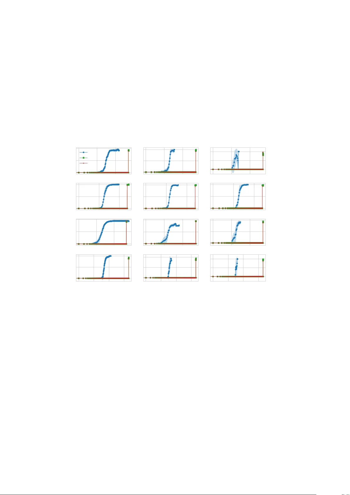
V ector Optimization with Gaussian Pro cess Bandits İlter Onat K orkmaz 1 , Y aşar Cahit Y ıldırım 1 , Çağın Ararat 1 , Cem T ekin 1* 1* Bilk en t Univ ersit y , Ank ara, Türkiy e. *Corresp onding author(s). E-mail(s): cem tekin@ee.bilken t.edu.tr ; Con tributing authors: onat.k orkmaz@bilk ent.edu.tr ; cahit.yildirim@bilk en t.edu.tr ; cararat@bilk en t.edu.tr ; Abstract W e study blac k-b o x v ector optimization with Gaussian pro cess bandits, where there is an incomplete order relation on ob jective vectors describ ed by a p oly- hedral con vex cone. Existing black-box vector optimization approac hes either suﬀer from high sample complexity or lack theoretical guaran tees. W e prop ose V e ctor Optimization with Gaussian Pr o c ess (V OGP), an adaptiv e elimination algorithm that identiﬁes P areto optimal solutions sample eﬃciently by exploiting the smo othness of the ob jectiv e function. W e establish theoretical guarantees, deriving information gain-based and k ernel-sp eciﬁc sample complexity bounds. Finally , we conduct a thorough empirical ev aluation of VOGP and compare it with the state-of-the-art multi-ob jective and v ector optimization algorithms on sev eral real-world and synthetic datasets, emphasizing V OGP’s eﬃciency ( e.g. , ∼ 18 × lo wer sample complexit y on av erage). W e also pro vide heuristic adap- tations of VOGP for cases where the design space is contin uous and where the Gaussian pro cess model lacks access to the true k ernel hyperparameters. This work op ens a new fron tier in sample-eﬃcient m ulti-ob jective blac k-b ox optimization b y incorp orating preference structures while maintaining theoretical guarantees and practical eﬃciency . Keyw ords: V ector optimization, ordering cones, Gaussian pro cess bandits, Bay esian optimization, sample complexity bounds 1 1 In tro duction In div erse ﬁelds suc h as engineering, economics, and computational biology , the problem of identifying the b est set of designs across multiple black-box ob jectives is a recurren t c hallenge. Often, the ev aluation of a particular design is b oth exp ensiv e and noisy , leading to the need for eﬃcient and reliable optimization metho ds. This issue is exempliﬁed in ﬁelds lik e aerospace engineering and drug discov ery , where each ev aluation can inv olv e costly exp erimen ts or simulations ( Muk aidaisi, V u, Gran tham, T chagang, & Li , 2022 ; Oba yashi, Y amaguchi, & Nak am ura , 1997 ). A common framew ork for dealing with suc h m ulti-ob jective optimization problems is to fo cus on identifying P areto optimal designs, for which there are no other designs that are b etter in all ob jectives. How ev er, this approach can b e restrictiv e, as it only p ermits a certain set of trade-oﬀs b et w een ob jectives where a disadv antage on one ob jective cannot b e comp ensated b y adv antages on other ob jectives, i.e., the domination relation requires sup eriorit y in all dimensions. A more comprehensive solution to this issue lies in vector optimization, where the partial ordering relations induced by conv ex cones are used. The core idea is to deﬁne a “cone” in the ob jective space that represents preferred directions of impro v ement. A solution is considered b etter than another if the vector diﬀerence b et ween their ob jectives falls within this preference cone. The use of ordering cones in this wa y gives users a framework that can model a wide range of trade-oﬀ preferences ( Jahn , 2010 ). Consider the c hallenge of optimizing the reactor parameters for n ucleophilic aro- matic substitution (SnAr) reaction, an imp ortant pro cess in synthetic c hemistry ( Grant et al. , 2018 ; T ak ao & Inagaki , 2022 ). In this scenario, the goal is to maximize the space-time yield and minimize the w aste-to-pro duct ratio, i.e., the E-factor. 1 Consider t wo designs where one of the designs has sligh tly less space-time yield and a muc h lo wer E-factor. A reasonable preference would b e to opt for the design that signiﬁcan tly reduces environmen tal impact, provided that the loss in space-time yield is not to o substan tial. Similarly , c ho osing designs that oﬀer considerably higher space-time yield, alb eit with a slightly increased en vironmen tal fo otprin t, might also be justiﬁed. In v ector optimization, this preference can b e enco ded with an obtuse cone (Figure 1 ). The regular Pareto optimality concept falls short in conv eying such preferences as it requires sup eriorit y in all ob jectives for domination relations. In Figure 1 , it can be seen that some of the designs (sho wn in red) in the Pareto front of traditional multi- ob jective order are not in the obtuse cone-based Pareto front, i.e., they are dominated b y designs that are m uch b etter in one ob jective and slightly w orse in the other. The example we just discussed demonstrates vector optimization within a t wo- dimensional ob jective space, as this low er dimensionality allo ws for straightforw ard visualization. How ever, when extending to higher dimensions, the structure of the p olyhedral cone ma y b e more intricate with high n um b er of faces. This is exempliﬁed b y Figure 2 , which shows a polyhedral cone with six faces in three dimensions. Such cones are not uncommon in the literature. F or example, Hunt, Wiecek, and Hughes ( 2010 ) pro vide a mo del of relativ e importance where allo wable trade-oﬀs betw een pairs of (p ossibly man y) ob jectives are giv en. They provide a complete algebraic 1 W e provide exp erimen ts on this optimization task in Section 6 . 2 θ ◦ Y ield − E f actor i / ∈ P ∗ ∪ P ∗ π/ 2 i ∈ P ∗ i ∈ P ∗ π/ 2 \ P ∗ Fig. 1 : V ector optimization on nucleophilic aromatic substitution (SnAr) reaction data ( Hone et al. , 2017 ). (Left) The ordering cone. (Right) Cone-sp eciﬁc Pareto front ( P ∗ ) and its comparison to P areto fron t of the comp onen t wise order ( P ∗ π / 2 ). Fig. 2 : A 3D cone. c haracterization of the cones corresponding to these kinds of preferences and sho w that they result in highly faceted polyhedral cones. While there exists previous w ork addressing P areto set identiﬁcation with resp ect to an ordering cone in noisy en vironments with theoretical guarantees ( Ararat & T ekin , 2023 ; Karagözlü, Yıldırım, Ararat, & T ekin , 2024 ), they tend to require v ast amounts of samples from the ob jective function, making them impractical in real-world scenarios. In this pap er, we address the problem of iden tifying the Pareto set with respect to an ordering cone C from a given set of designs with a minim um n umber of noisy black-box function queries. W e propose V e ctor Optimization with Gaussian Pr o c ess (V OGP), an ( ϵ, δ )- pr ob ably appr oximately c orr e ct (P A C) adaptive elimination algorithm that p erforms black-box v ector optimization by utilizing the mo deling p o wer of Gaussian pro cesses (GPs). In particular, V OGP lev erages conﬁdence regions formed by GPs to p erform cone-dep enden t, probabilistic elimination and Pareto identiﬁcation steps, whic h adaptively explore the Pareto front with Bay esian optimization ( Garnett , 2023 ). Similar to P areto Activ e Learning (P AL) and ϵ -P AL ( Zuluaga, Krause, & Püschel , 2016 ; Zuluaga, Sergent, Krause, & Püschel , 2013 ) for the multi-ob jectiv e case (see next subsection), VOGP op erates in a fully exploratory setting, where the least certain design is queried at eac h round. When V OGP is considered with the sp ecial case of comp onen twise order (p ositiv e orthant cone in vector optimization), it can b e seen as 3 a v ariant of P AL and ϵ -P AL that can handle correlated ob jectives. W e prov e strong theoretical guaran tees on the conv ergence of VOGP and derive information gain-based sample complexity b ounds. Our main contributions can b e listed as follo ws: • W e prop ose VOGP , an ( ϵ, δ )-P AC adaptive elimination algorithm that p erforms v ector optimization by utilizing GPs. This is the ﬁrst w ork to provide a theoretical foundation for vector optimization within the framew ork of GP bandits. • When the design set is ﬁnite, we theoretically prov e that VOGP returns an ( ϵ, δ )-P AC P areto set with a cone-dep enden t sample complexit y b ound in terms of the maxim um information gain. W e also provide explicit kernel-speciﬁc sample complexity b ounds. • W e empirically sho w that V OGP satisﬁes the theoretical guarantees across diﬀeren t datasets and ordering cones. W e also demonstrate that VOGP outp erforms existing metho ds on v ector optimization and its sp ecial case, multi-ob jectiv e optimization. • W e extend VOGP to w ork on contin uous design sets by using tree-based adaptive discretization tec hniques. W e empirically ev aluate this extension in con tin uous design sets. W e also study a heuristic v ariant of VOGP to handle the case of unknown GP k ernel hyperparameters. 2 Related W ork There is considerable existing w ork on P areto set identiﬁcation that utilizes GPs ( Candelieri, Pon ti, & Archetti , 2024 ; Emmeric h, Deutz, & Klink enberg , 2011 ; Lyu, Y ang, Y an, Zhou, & Zeng , 2018 ; Mathern et al. , 2021 ; Pic hen y , 2013 ; Shu, Jiang, Shao, & W ang , 2020 ; Suzuki, T ak eno, T amura, Shitara, & Karasuyama , 2020 ; Svenson & San tner , 2016 ). Some of these works use information-theoretic acquisition functions. F or instance, PESMO tries to sample designs that optimize the mutual information b et ween the observ ation and the P areto set, given the dataset ( Hernandez-Lobato, Hernandez-Lobato, Shah, & A dams , 2016 ). MESMO tries to sample designs that maximize the m utual information b etw een observ ations and the P areto front ( Belak aria, Desh wal, & Doppa , 2019 ). JES tries to sample designs that maximize the mutual information b et ween observ ations and the join t distribution of the Pareto set and P areto fron t ( T u, Gandy , Kantas, & Shafei , 2022 ). Diﬀerent from entrop y search-based metho ds, some other metho ds utilize high-probability conﬁdence regions formed by the GP p osterior. F or instance, P ALS ( Barracosa et al. , 2022 ), P AL and ϵ -P AL are conﬁdence region-based adaptiv e elimination algorithms that aim to categorize the input data points into three groups using the mo dels they hav e learned: those that are P areto optimal, those that are not Pareto optimal, and those whose statuses are uncertain ( Zuluaga et al. , 2016 , 2013 ). In every iteration, these algorithms choose a p oten tial design for ev aluation with the aim of reducing the quantit y of data p oin ts in the uncertain category . Thanks to GP-based mo deling, a substantial n umber of designs can b e explored b y a single query . Assuming indep endent ob jectives, P AL and ϵ -P AL work in the ﬁxed conﬁdence setting and hav e a v ariable sampling budget. On the other hand, entrop y search-based metho ds are often in vestigated in ﬁxed-budget setting without any theoretical guarantees on the accuracy of Pareto set identiﬁcation. Ho wev er, all the algorithms mentioned ab o ve try to iden tify the Pareto set with resp ect 4 to the comp onen twise order. They are not able to incorp orate user preferences enco ded b y ordering cones. In the context of multi-ob jectiv e Bay esian optimization, there is a limited amount of work that incorp orates user preferences. Ab dolshah, Shilton, Rana, Gupta, and V enk atesh ( 2019 ) propose M OBO-PC, a multi-ob jective Bay esian optimization algo- rithm which incorp orates user preferences in the form of preference-order constrain ts. MOBO-PC uses exp ected Pareto h yp erv olume improv emen t weigh ted by the proba- bilit y of ob eying preference-order constraints as its acquisition function. K. Y ang, Li, Deutz, Bac k, and Emmerich ( 2016 ) prop ose a method that uses truncated exp ected h yp erv olume imp ro vemen t and considers the predictiv e mean, v ariance, and the pre- ferred region in the ob jective space. Some works employ preference learning ( Bemp orad & Piga , 2021 ; Chu & Ghahramani , 2005a ; Hak anen & Kno wles , 2017 ; Ignatenko, K ondrashov, Cox, & de V ries , 2021 ; T aylor, Ha, Li, Chan, & Li , 2021 ; Ungredda & Brank e , 2023 ), where the user interacts sequentially with the algorithm to learn the user preference ( Astudillo & F razier , 2019 ; Lin, Astudillo, F razier, & Bakshy , 2022 ). Astudillo and F razier ( 2019 ) emplo y Bay esian preference learning where the user’s preferences are mo deled as a utilit y function and they prop ose tw o nov el acquisition functions that are robust to utility uncertain ty . Lin et al. ( 2022 ) consider v arious preference exploration metho ds while also representing user preferences with a utility function which is mo deled with a GP . Ahmadianshalc hi, Belak aria, and Doppa ( 2024 ) prop ose P A C-MOO, a constrained multi-ob jectiv e Ba yesian optimization algorithm whic h incorp orates preferences in the form of weigh ts that add up to one. P AC-MOO uses the information gained ab out the optimal constrained Pareto front w eighted by preference weigh ts as its acquisition function. Khan, Dietric h, and Wirth ( 2022 ) pro- p ose a metho d that learns a utility function oﬄine b y using exp ert knowledge to a v oid the rep eated and exp ensiv e exp ert inv olvemen t. In the broader context of gradient-free optimization, zeroth-order optimization tec hniques hav e b een explored to handle optimization problems where gradient infor- mation is una v ailable ( Dang, Y ang, Liu, & Ruan , 2024 ). In the multi-ob jective case, n umerous studies employ evolutionary algorithms in order to estimate the Pareto front, thereb y accomplishing this task through the iterative developmen t of a p opulation of ev aluated designs ( Dang, Zhang, W ang, Y ang, & Zhan , 2023 , 2024 ; Deb, Pratap, Agarw al, & Meyariv an , 2002 ; Kno wles , 2006 ; Seada & Deb , 2015 ; Zhang & Li , 2007 ). Some of these metho ds use h yp erv olume calculation to guide their metho d ( Bader & Zitzler , 2011 ; Beume, Naujoks, & Emmeric h , 2007 ; Z. Y ang, W ang, Y ang, Back, & Emmerich , 2016 ). Dang, Zhang, et al. ( 2024 ) incorp orates generativ e adversarial net works into ev olutionary algorithms to impro v e oﬀspring diversit y in the context of m ultimo dal m ulti-ob jective optimization. Dang et al. ( 2023 ) uses m ulti-ob jective ev o- lutionary algorithms in federated learning for device selection, where m ulti-ob jective form ulation helps balance resource eﬃciency and test accuracy . There is a signiﬁcant b ody of research that deals with the integration of user preferences into multi-ob jectiv e ev olutionary algorithms ( Branke & Deb , 2005 ; Co ello , 2000 ; H. Li & Silv a , 2008 ; Phelps & Köksalan , 2003 ; Sinha, Korhonen, W allenius, & Deb , 2010 ; Zhou et al. , 2011 ). Using evolutionary algorithms, preferences can b e articulated a priori , a p oste- riori , or interactiv ely . V arious methods for expressing preferences hav e b een suggested, 5 primarily encompassing techniques based on ob jective comparisons, solution rank- ing, and exp ectation-based approaches ( Zhou et al. , 2011 ). There are also w orks that emplo y preference cones in multi-ob jectiv e ev olutionary algorithms. Batista, Campelo, Guimarães, and Ramírez ( 2011 ) utilize p olyhedral cones as a metho d of managing the resolution of the estimated Pareto fron t. F erreira, Meneghini, Brandao, and Guimarães ( 2020 ) apply preference cone-based multi-ob jectiv e evolutionary algorithm to optimize distributed energy resources in microgrids. There are techniques that transform a multi-ob jectiv e optimization problem into a single-ob jective problem by assigning w eights to the ob jectiv es ( Knowles , 2006 ; P onw eiser, W agner, Biermann, & Vincze , 2008 ). The transformed problem can b e solv ed using standard single-ob jective optimization metho ds. ParEGO introduced in Kno wles ( 2006 ) transforms the m ulti-ob jective optimization problem into a single- ob jective one by using T c heb ycheﬀ scalarization and solves it by Eﬃcient Global Optimization (EGO) algorithm, whic h was designed for single-ob jective exp ensiv e optimization problems. There are existing works that incorp orate p olyhedral structures to guide the design iden tiﬁcation task. As an example, Katz-Sam uels and Scott ( 2018 ) introduce the concept of feasible arm iden tiﬁcation. Their ob jectiv e is to identify arms whose av erage rew ards fall within a sp eciﬁed p olyhedron, using ev aluations that are sub ject to noise. Ararat and T ekin ( 2023 ) propose a Naïv e Elimination (NE) algorithm for P areto set iden tiﬁcation with p olyhedral ordering cones. They pro vide sample complexity b ounds on the ( ϵ , δ )-P AC Pareto set iden tiﬁcation p erformance of this algorithm. How ever, their algorithm assumes independent arms and do es not perform adaptiv e elimination. As a result, they only hav e worst-case sample complexit y bounds for this algorithm. Exp erimen ts show that identiﬁcation requires a large sampling budget which renders NE impractical in real-world problems of interest. Karagözlü et al. ( 2024 ) introduce the PaV eBa algorithm, designed for identifying Pareto sets using polyhedral ordering cones. They also establish sample complexity bounds for the ( ϵ , δ )-P AC Pareto set iden tiﬁcation task within bandit settings. How ever, their analysis lacks theoretical guaran tees when Gaussian pro cesses are employ ed. T able 1 : Comparison with Related W orks Paper Cone- based prefer- ences Sample complexity bounds ( ϵ , δ )- P A C Utilizes GPs Contin uous domain This work Y es Y es Y es Y es Y es Karagözlü et al. ( 2024 ) Y es Y es Y es No No Ararat and T ekin ( 2023 ) Y es Y es Y es No No T u et al. ( 2022 ) No No No Y es Y es Belak aria et al. ( 2019 ) No No No Y es Y es Hernandez-Lobato et al. ( 2016 ) No No No Y es Y es Zuluaga et al. ( 2016 ) No Y es Y es Y es No 6 T able 1 compares our work with the most closely related prior w orks in terms of key asp ects. An imp ortan t distinction is that our metho d supp orts cone-based preferences while also oﬀering theoretical sample complexity guaran tees in P AC framew ork. While Karagözlü et al. ( 2024 ) and Ararat and T ekin ( 2023 ) also incorporate cone-based preferences and pro vide sample complexit y b ounds, they do not utilize Gaussian pro cesses and are restricted to discrete domains. In contrast, information theoretic metho ds suc h as PESMO ( Hernandez-Lobato et al. , 2016 ), MESMO ( Belak aria et al. , 2019 ), and JES ( T u et al. , 2022 ) use Gaussian pro cesses and op erate in contin uous domains but do not oﬀer sample complexit y guarantees, nor do they incorp orate cone- based preferences. Zuluaga et al. ( 2013 ) employs Gaussian pro cesses but do es not incorp orate cone-based preferences, and is also restricted to discrete domains. 3 Bac kground and problem deﬁnition The aim of this w ork is to incorporate p olyhedral cones as preference structures to guide the multi-ob jectiv e optimization, while maintaining theoretical guaran tees and practical eﬃciency . F ormally , we consider the problem of sequentially maximizing a v ector-v alued function f : X → R M o ver a ﬁnite set of designs 2 X ⊂ R D with resp ect to a p olyhedral ordering cone C ⊂ R M . In each iteration t , a design p oin t x t is selected, and a noisy observ ation is recorded as y t = f ( x t ) + ν t . Here, the noise comp onent ν t has the multiv ariate Gaussian distribution N  0 , σ 2 I M × M  , where σ 2 denotes the v ariance of the noise. T o deﬁne the optimalit y of designs, we use the partial order induced by C . A detailed table of notations can b e found in App endix A . 3.1 P artial order induced b y a cone The partial order among designs is induced by a kno wn p olyhedral ordering cone C ⊆ R M , that is, a p olyhedral closed con v ex cone whose interior, denoted b y in t ( C ) , is nonempt y with C ∩− C = { 0 } . Suc h a cone can b e written as C =  x ∈ R M | W x ≥ 0  , where W is a N × M matrix, N is the num b er of halfspaces that deﬁne C , and N ≥ M . Without loss of generality , the ro ws w ⊤ 1 , . . . , w ⊤ N are assumed to b e unit normal vectors of these halfspaces with resp ect to the Euclidean norm ∥ · ∥ 2 . F or r ≥ 0 , we write B ( r ) : = { y ∈ R M | ∥ y ∥ 2 ≤ r } . W e say that y ∈ R M w eakly dominates y ′ ∈ R M with resp ect to C if their diﬀerence lies in C : y ′ ≼ C y ⇔ y − y ′ ∈ C . By the structure of C , an equiv alent expression is: y ′ ≼ C y ⇔ w ⊤ n ( y − y ′ ) ≥ 0 , ∀ n ∈ [ N ] := { 1 , . . . , N } . (1) Moreo ver, we say that y strictly dominates y ′ with resp ect to C if their diﬀerence lies in in t ( C ) : y ′ ≺ C y ⇔ y − y ′ ∈ int ( C ) . This is equiv alent to: y ′ ≺ C y ⇔ w ⊤ n ( y − y ′ ) > 0 , ∀ n ∈ [ N ] . Similarly , w e write y ′ ≼ C \{ 0 } y ⇔ y − y ′ ∈ C \ { 0 } to exclude the case where the t wo vectors coincide. The P areto set with respect to cone C is the set of 2 Extension to contin uous case is discussed in Section 6 . 7 designs that are not weakly dominated b y any other design with respect to C giv en as P ∗ := P ∗ C := { x ∈ X | ∄ x ′ ∈ X : f ( x ) ≼ C \{ 0 } f ( x ′ ) } . Example 1 Consider a scenario with tw o ob jectives ( M = 2) , denoted by f 1 and f 2 . In this example, we assume that f 2 is prioritized ov er f 1 , meaning the user is willing to trade oﬀ some amount of f 1 for a suﬃcient gain in f 2 . Figure 3 illustrates the corresp onding preference cone, where the red square is preferred ov er the blue circle. This preference structure diﬀers from the component wise order, under which these designs would b e incomparable. f 1 f 2 (Priority ob jective) ≼ C  ≼ R 2 + Fig. 3 : Visualization of a t wo-dimensional cone that prioritizes the f 2 ob jective. Unlik e the comp onen twise order, the cone order establishes a domination relation b y prioritizing f 2 . The dominance relation under the preference cone is evident, as the diﬀerence of red square from blue circle lies inside the cone , conﬁrming that the red square is preferred according to this ordering. R emark 1 The relation ≼ C induced by the cone C is a vector preorder on R N that is non- total (incomplete). The c hoice C = R M + corresp onds to the usual comp onen twise order i n m ulti-ob jective optimization. In general, using a larger cones results in a smaller Pareto set; we refer the reader to Ararat and T ekin ( 2023 , Remark 2.3) for possible uses of larger cones in small molecule drug discov ery problem. In multi-asset markets with prop ortional transaction costs in ﬁnance, C can b e chosen as the so-called solv ency cone determined by the transaction costs rates; see Kabano v ( 1999 ). Cone-induced preorders form an imp ortan t sp ecial class of preorders. The underlying scaling prop ert y , enco ded by C b eing a cone, is a strong assumption whose suitability should be justiﬁed in the particular application. F or instance, in the case of solvency cones, the assumption that the transaction costs are incurred in prop ortion to the v olume at a ﬁxed rate justiﬁes the use of a cone naturally . 8 R emark 2 In this pap er, we assume that the non-total order relation ≼ C is given a priori and the optimization task is performed with resp ect to it. A diﬀeren t strand of literature fo cuses on the problem of le arning the underlying order relation from data; see, e.g., Audiﬀren and Ralaiv ola ( 2017 ); Chau, Gonzalez, and Sejdino vic ( 2022 ); Chu and Ghahramani ( 2005b ); Y ue, Bro der, Klein b erg, and Joachims ( 2012 ). Since the focus of the current paper is optimization with resp ect to a known vector preorder, the approach of these references is orthogonal to our work. 3.2 ( ϵ, δ ) -P AC P areto set W e use the cone-dep endent, direction-free sub optimalit y gaps deﬁned in Ararat and T ekin ( 2023 ). The gap b et ween designs x, x ′ ∈ X is giv en as m ( x, x ′ ) := inf { s ≥ 0 | ∃ u ∈ B (1) ∩ C : f ( x ) + s u / ∈ f ( x ′ ) − int( C ) } , the − op eration on sets is the Minko wski diﬀerence (vectors b eing treated as singletons). The sub optimalit y gap of design x is deﬁned as ∆ ∗ x := max x ′ ∈ P ∗ m ( x, x ′ ) . Deﬁnition 1. Let ϵ > 0 , δ ∈ (0 , 1) . A random set P ⊆ X is called an ( ϵ, δ ) -P AC Par eto set if the subsequent conditions are satisﬁed at least with probability 1 − δ : (i) S x ∈ P ( f ( x ) + B ( ϵ ) ∩ C − C ) ⊇ S x ∈ P ∗ ( f ( x ) − C ) ; (ii) ∀ x ∈ P \ P ∗ : ∆ ∗ x ≤ 2 ϵ . R emark 3 Condition (i) of Deﬁnition 1 is equiv alent to the following: F or every x ∗ ∈ P ∗ , there exist x ∈ P and u ∈ B ( ϵ ) ∩ C suc h that f ( x ∗ ) ≼ C f ( x ) + u . Even though certain designs in P ma y not b e optimal, condition (ii) of Deﬁnition 1 limits the exten t of the inadequacies in these designs. Consequen tly , it ensures the ov erall qualit y of all the designs pro duced. Our aim is to design an algorithm that returns an ( ϵ, δ ) -P AC Pareto set ˆ P ⊆ X with as little sampling from the expensive ob jective function f as p ossible. 3.3 Mo deling of the ob jective function W e mo del the ob jective function f as a realization of an M -output GP with zero mean and a p ositiv e deﬁnite co v ariance function k with b ounded v ariance: k j j ( x, x ) ≤ 1 for ev ery x ∈ X and j ∈ [ M ] . Let ˜ x i b e the i th design observed and y i the corresp onding observ ation. The posterior distribution of f conditioned on the ﬁrst t observ ations is that of an M -output GP with mean ( µ t ) and cov ariance ( k t ) functions given b elo w, where k t ( x ) = [ k ( x, x 1 ) , . . . , k ( x, x t )] ∈ R M × M t , y [ t ] =  y ⊤ 1 , . . . , y ⊤ t  ⊤ , K t = ( k ( x i , x j ) ) i,j ∈ [ t ] , and I M t is the M t × M t identit y matrix: µ t ( x ) = k t ( x )  K t + σ 2 I M t  − 1 y ⊤ [ t ] , (2) k t ( x, x ′ ) = k ( x, x ′ ) − k t ( x )  K t + σ 2 I M t  − 1 k t ( x ′ ) ⊤ . (3) 9 Our sample complexity results will depend on the diﬃculty of learning f , which is c haracterized by its maxim um information gain. Deﬁnition 2. The maxim um information gain at round t is deﬁned as γ t : = max A ⊆X : | A | = t I( y A ; f A ) , where y A is the collection of observ ations corresponding to the designs in A , f A is the collection of the corresp onding function v alues, and I( y A ; f A ) is the mutual information b et ween the t wo. 4 Metho d W e prop ose V e ctor Optimization with Gaussian Pr o c ess (V OGP), an ( ϵ, δ )-P AC adap- tiv e elimination algorithm that p erforms vector optimization b y utilizing the mo deling p o wer of GPs (see Algortihm 1 ). VOGP tak es as input the design set X , cone C , accuracy parameter ϵ , and conﬁdence parameter δ . V OGP adaptiv ely classiﬁes designs as sub optimal, Pareto optimal, and uncertain. Initially , all designs are put in the set of uncertain designs, denoted b y S t . Designs that are classiﬁed as sub optimal are dis- carded and never considered again in comparisons, making it sample-eﬃcien t. Designs that are classiﬁed as Pareto optimal are mov ed to the predicted Pareto set ˆ P t . VOGP trac ks the set of active designs by assigning them to A t b efore discarding and W t afterw ards. VOGP terminates and returns ˆ P = ˆ P t when the set of uncertain designs b ecomes empty . Decision-making in each round is divided into four phases named mo deling , disc ar ding , Par eto identiﬁc ation , evaluating . Below, we describ e each phase in detail. Algorithm 1 VOGP Input: Design set X , ϵ ≥ 0 , δ ∈ (0 , 1) , polyhedral ordering cone C , kernel k Initialize: Predicted Pareto set P 1 = ∅ , set of uncertain designs S 1 = X , sets of activ e designs A 1 = ∅ and W 1 = ∅ , R 0 ( x ) = R M for each x ∈ S 1 , t = 1 Compute: Accuracy vector u ∗ ∈ C given in Deﬁnition 4 while S t  = ∅ do Run Modeling ( S t , P t ) in Algorithm 2 Run Discarding ( S t , A t ) in Algorithm 3 Run P aretoIdentifica tion ( S t , P t ) in Algorithm 4 Run Ev alua ting ( S t , W t ) in Algorithm 5 P t +1 = P t , S t +1 = S t t = t + 1 end while return Predicted Pareto set ˆ P = P t R emark 4 Our theoretical results, similar to other theoretical w orks related to ours ( Sriniv as, Krause, Kak ade, & Seeger , 2012 ; Zuluaga et al. , 2013 ), assume that the kernel is known and ﬁxed. In practice, how ever, the k ernel may b e unknown and must b e estimated from data concurren tly with the decision-making pro cess; see, e.g., Berk enk amp, Sc ho ellig, and Krause 10 ( 2019 ); Ziomek, Adac hi, and Osb orne ( 2024 ). W e discuss this practical case in Section 6.5 , where we pro vide an empirical adaptation of Algorithm 1 for unknown h yp erparameters. 4.1 Mo deling This phase is summarized in Algorithm 2 . V OGP uses the GP posterior means and v ariances of designs to deﬁne conﬁdence regions in the form of M -dimensional h yp errectangles whic h are scaled b y β t , a function of the conﬁdence parameter δ . The probabilit y that these h yp errectangles include the true ob jectiv e v alues of the designs is at least 1 − δ . Using these conﬁdence h yp errectangles allows for the form ulation of probabilistic success criteria and the quantiﬁcation of uncertaint y with designs. A t eac h round t , the h yp errectangle Q t ( x ) = { y ∈ R M | µ j t ( x ) − β 1 / 2 t σ j t ( x ) ≤ y j ≤ µ j t ( x ) + β 1 / 2 t σ j t ( x ) , ∀ j ∈ [ M ] } (4) is computed for design x , where β t = 2 ln  M π 2 |X | t 2 / (3 δ )  . Algorithm 2 Mo deling Subroutine Compute: Set of active designs A t = S t ∪ P t ; for x ∈ A t do Obtain GP p osterior for x : µ t ( x ) and σ t ( x ) given in Equation 2 ; Construct conﬁdence hyperrectangle Q t ( x ) given in Equation 4 ; R t ( x ) = R t − 1 ( x ) ∩ Q t ( x ) ; end for Moreo ver, all the calculated h yp errectangles up to round t are intersected cum ulatively to obtain the cum ulativ e conﬁdence hyperrectangle R t ( x ) of design x . 4.2 Discarding This phase is summarized in Algorithm 3 . VOGP discards undecided designs that are dominated with resp ect to C with high probability . The designs that are to b e discarded with low probability are identiﬁed and are used to form the p essimistic P areto set P ( C ) pess ,t ( A t ) as deﬁned b elo w. The illustration of discarding phase can b e seen in Figure 4 (Left, Middle). Deﬁnition 3 (Pessimistic Pareto Set) . Let t ≥ 1 and let D ⊆ A t b e a nonempt y set of no des. The p essimistic Par eto set of D with resp ect to C at round t , denoted by P ( C ) pess ,t ( D ) , is the set of all nodes x ∈ D for whic h there is no no de x ′ ∈ D suc h that R t ( x ′ ) + C ⊊ R t ( x ) + C . 11 Algorithm 3 Discarding Subroutine Compute: P pess ,t = P ( C ) pess ,t ( A t ) as in Deﬁnition 3 for x ∈ S t \ P pess ,t do if ∃ x ′ ∈ P pess ,t ∀ y ∈ R t ( x ) : R t ( x ′ ) + ϵ u ∗ ⊆ y + C then S t = S t \ { x } ; end if end for R emark 5 In the setting of Deﬁnition 3 , P ( C ) pess ,t ( D ) can b e seen as the set of all no des that yield maximal elemen ts of a certain partial order relation on sets. Indeed, for A, A ′ ⊆ R M , let us write A ′ ⪯ C A if and only if A ′ ⊆ A + C , which holds if and only if A ′ + C ⊆ A + C . Then, it is easy to chec k that the set relation ⪯ C is a preorder, i.e., a reﬂexiv e and transitive binary relation, on the pow er set of R M . Let ∼ C denote the symmetric part of this relation, i.e., A ′ ∼ C A if and only if A ′ ⪯ C A and A ⪯ C A ′ , which holds if and only if A ′ + C = A + C . Then, ∼ C is an equiv alence relation on the p o wer set of R M and the set of equiv alence classes can b e identiﬁed b y the collection M C := { A ⊆ R M | A = A + C } . Then, M C is a partially ordered set with resp ect to ⪯ C and the relation ⪯ C coincides with the usual ⊆ relation on M C . It then follows that P ( C ) pess ,t ( D ) is the set of all no des x ∈ D for which R t ( x ) + C is a maximal elemen t of { R t ( x ′ ) + C | x ′ ∈ A t } with respect to ⪯ C . In particular, since every ﬁnite nonempty partially ordered set has a maximal element, we hav e P ( C ) pess ,t ( D )  = ∅ . The reader is referred to Hamel, Heyde, Löhne, Rudloﬀ, and Sc hrage ( 2015 , Section 2.1) for more details on set relations. V OGP computes p essimistic Pareto set of A t b y chec king for eac h design in A t whether there is another design that prev en ts it from b eing in the p essimistic Pareto set. T o see if design x prev ents design x ′ from b eing in the p essimistic P areto set, by solving a con vex optimization problem, V OGP chec ks if every v ertex of R t ( x ′ ) can b e expressed as the sum of a v ector in C and a vector in R t ( x ) . VOGP reﬁnes the undecided set by utilizing the p essimistic Pareto set. It eliminates designs based on the follo wing criteria: for a given design x , if all v alues inside its conﬁdence h yp errectangle, when added to an "accuracy v ector" ϵ u ∗ , are dominated with resp ect to C b y all v alues in the conﬁdence h yp errectangle of another design x ′ , then the dominated design x is discarded. The dominating design x ′ should be a member of the p essimistic Pareto set. Deﬁnition 4. Let A C : = T u ∈ S M − 1 ( u + C ) and d C : = inf {∥ z ∥ 2 | z ∈ A C } . Then, there exists a unique vector z ∗ ∈ A C suc h that d C = ∥ z ∗ ∥ 2 and we deﬁne u ∗ : = z ∗ d C . Lemma 1. L et y , z ∈ R M and ˜ p ∈ B ( ϵ d C ) . 1. If y + ˜ p ≼ C z , then y ≼ C z + ϵ u ∗ . 2. If ˜ p ∈ int( B ( ϵ d C )) and y + ˜ p ≼ C z , then y ≺ C z + ϵ u ∗ . Due to its tec hnical nature, the pro of of Lemma 1 is given in Section 5.1 along with the pro ofs of several other technical lemmas. 12 f 1 f 2 f ( x 1 ) f ( x 2 ) f ( x 3 ) x 1 / ∈ P pess,t . f 1 f 2 ϵ ϵ ϵ ϵ f ( x 2 ) f ( x 1 ) f ( x 3 ) x 1 is discarded. f 1 f 2 f ( x 2 ) ϵ ϵ ϵ ϵ f ( x 3 ) x 2 is not identiﬁed as Pareto. x 3 is identiﬁed as Pareto. Fig. 4 : (Left, Middle) Visualization of discarding, and (Right) Pareto identiﬁcation phases of VOGP in tw o dimensional ob jective space. Note that all b o xes corresp ond to the R t ( x i ) for corresp onding true ob jective v alues f ( x i ) for i = 1 , 2 , 3 . In this simple case, in the middle plot, the intersection of the tw o cones are equiv alent to the in tersection of all cones coming out of R t ( x 1 ) . R emark 6 d C corresp onds to the magnitude of the smallest translation of a unit sphere so that the whole unit sphere is inside the cone C (i.e., so that the origin dominates the unit sphere). u ∗ is the direction of this smallest translation. d C quan tiﬁes how hard it is to reach to a domination relation when using a sp eciﬁc ordering cone. W e call this term the or dering har dness of cone C . 4.2.1 Computation of the p essimistic Pareto set Let t ∈ N . According to Deﬁnition 3 , to c hec k if a design x ∈ A t is included in P pess ,t , the condition R t ( x ′ ) + C ⊊ R t ( x ) + C needs to b e chec ked for every x ′ ∈ A t . W e ﬁrst formulate this condition in terms of conv ex feasibility problems. These problems can also b e expressed as conv ex optimization problems whose ob jective functions are zero and we solve them n umerically using the CVXPY library ( Agraw al, V ersch ueren, Diamond, & Boyd , 2018 ; Diamond & Bo yd , 2016 ). Let x, x ′ ∈ A t . Since R t ( x ′ ) is a conv ex polytop e, we hav e R t ( x ′ ) + C ⊆ R t ( x ) + C ⇐ ⇒ R t ( x ′ ) ⊆ R t ( x ) + C ⇐ ⇒ ∀ v ′ ∈ vert( R t ( x ′ )) : v ′ ∈ R t ( x ) + C ⇐ ⇒ ∀ v ′ ∈ vert( R t ( x ′ )) ∃ y ∈ R t ( x ) : y ≼ C v ′ . Hence, for eac h v ′ ∈ vert ( R t ( x ′ )) , w e chec k the condition ∃ y ∈ R t ( x ) : y ≼ C v ′ b y solving the following conv ex feasibility problem: minimize y 0 sub ject to y ∈ R M , y j ≥ µ j s ( x ) − β 1 / 2 s σ j s ( x ) , ∀ j ∈ [ M ] , ∀ s ∈ [ t ] y j ≤ µ j s ( x ) + β 1 / 2 s σ j s ( x ) , ∀ j ∈ [ M ] , ∀ s ∈ [ t ] w T n y ≤ w T n v ′ , ∀ n ∈ [ N ] . ( F t ( x, v ′ ) ) 13 Moreo ver, under the condition R t ( x ′ ) + C ⊆ R t ( x ) + C , we hav e R t ( x ′ ) + C  = R t ( x ) + C ⇐ ⇒ R t ( x ) ⊆ R t ( x ′ ) + C ⇐ ⇒ ∃ v ∈ vert( R t ( x )) : v / ∈ R t ( x ′ ) + C ⇐ ⇒ ∃ v ∈ vert( R t ( x ))  ∃ y ′ ∈ R t ( x ′ ) : y ′ ≼ C v . Hence, for eac h v ∈ v ert ( R t ( x )) , w e chec k the condition ∃ y ′ ∈ R t ( x ′ ) : y ′ ≼ C v b y solving ( F t ( x ′ , v ) ) deﬁned in the same wa y: minimize y ′ 0 sub ject to y ′ ∈ R M , ( y ′ ) j ≥ µ j s ( x ′ ) − β 1 / 2 s σ j s ( x ′ ) , ∀ j ∈ [ M ] , ∀ s ∈ [ t ] ( y ′ ) j ≤ µ j s ( x ′ ) + β 1 / 2 s σ j s ( x ′ ) , ∀ j ∈ [ M ] , ∀ s ∈ [ t ] w T n y ′ ≤ w T n v , ∀ n ∈ [ N ] . ( F t ( x ′ , v ) ) Hence, if there exists x ′ ∈ A t suc h that ( F t ( x, v ′ ) ) is feasible for every v ′ ∈ vert ( R t ( x ′ )) and ( F t ( x ′ , v ) ) is infeasible for at least one v ∈ v ert ( R t ( x )) , then x is not added to P pess ,t . Otherwise, x is added to P pess ,t . 4.2.2 Computation of discarded designs In its original form, the discarding criteria of VOGP (see Algorithm 3 ) requires c hecking domination relations b et ween inﬁnitely man y p oint pairs from tw o conﬁdence h yp errectangles. In this section, we show that the suﬃcient num b er of chec ks can b e reduced signiﬁcantly by considering only the vertex pairs of the hyperrectangles, allo wing for an eﬃcient implementation. This is achiev ed thanks to the next lemma. F or a nonempt y conv ex polytop e A ⊆ R M , we denote by v ert ( A ) its set of all vertices. Lemma 2. L et x, x ′ ∈ X and t ∈ N . F or the cumulative c onﬁdenc e hyp err e ctangles R t ( x ) , R t ( x ′ ) , the fol lowing statements ar e e quivalent. (i) ∀ y ∈ R t ( x ) ∀ y ′ ∈ R t ( x ′ ) : y ≼ C y ′ . (ii) ∀ v ∈ v ert( R t ( x )) ∀ v ′ ∈ vert( R t ( x ′ )) : v ≼ C v ′ . Pr o of. It is clear that (i) implies (ii) since v ert ( R t ( x )) ⊆ R t ( x ) and v ert ( R t ( x ′ )) ⊆ R t ( x ′ ) . T o show the reverse implication, supp ose that (ii) holds; let y ∈ R t ( x ) and y ′ ∈ R t ( x ′ ) . W e proceed in t wo steps. First, let us further assume that y ∈ v ert ( R t ( x )) . Moreov er, since y ′ ∈ R t ( x ′ ) and R t ( x ′ ) is a conv ex polytop e, we may write y ′ = X v ′ ∈ vert( R t ( x ′ )) λ v ′ v ′ , 14 where λ v ′ ≥ 0 for each v ′ ∈ vert( R t ( x ′ )) such that X v ′ ∈ vert( R t ( x ′ )) λ v ′ = 1 . Note that (ii) implies that ∀ v ′ ∈ vert( R t ( x ′ )) : y ≼ C v ′ , whic h implies that ∀ v ′ ∈ vert( R t ( x ′ )) : λ v ′ y ≼ C λ v ′ v ′ . Then, summing ov er all v ′ ∈ vert( R t ( x ′ )) yields y = X v ′ ∈ vert( R t ( x ′ )) λ v ′ y ≼ C X v ′ ∈ vert( R t ( x ′ )) λ v ′ v ′ = y ′ . Hence, (i) holds in this step. Next, we consider the general case, where y ∈ R t ( x ) . Since R t ( x ) is a conv ex p olytope, we ma y write y = X v ∈ v ert( R t ( x )) α v v , where α v ≥ 0 for each v ∈ v ert( R t ( x )) such that X v ∈ v ert( R t ( x )) α v = 1 . By the ﬁrst step, we ha ve ∀ v ∈ v ert( R t ( x )) : v ≼ C y ′ . Then, we obtain ∀ v ∈ v ert( R t ( x )) : α v v ≼ C α v y ′ . Finally , summing o ver all v ∈ vert( R t ( x )) yields y = X v ∈ v ert( R t ( x )) α v v ≼ C X v ∈ v ert( R t ( x )) α v y ′ = y ′ . Hence, (i) holds in the general case to o. □ Let t ∈ N . In Algorithm 3 , to decide if a design x ∈ S t is going to be discarded, the condition ∃ x ′ ∈ P pess ,t ∀ y ∈ R t ( x ) : R t ( x ′ ) + ϵ u ∗ ⊆ y + C needs to b e chec ked, whic h requires en umerating all designs in P pess ,t . Giv en x ′ ∈ P pess ,t , observ e that ∀ y ∈ R t ( x ) : R t ( x ′ ) + ϵ u ∗ ⊆ y + C ⇐ ⇒ ∀ y ∈ R t ( x ) ∀ y ′ ∈ R t ( x ′ ) : y ≼ C y ′ + ϵ u ∗ 15 ⇐ ⇒ ∀ y ∈ R t ( x ) ∀ ¯ y ∈ R t ( x ′ ) + ϵ u ∗ : ¯ y ≼ C y . Hence, the last condition can be c heck ed equiv alen tly instead of the original condition. Notice that R t ( x ′ ) + ϵ u ∗ is a shifted h yp errectangle, which is also a h yp errectangle. Therefore, by Lemma 2 , the abov e conditions are also equiv alen t to the following: ∀ v ∈ v ert( R t ( x )) , ∀ v ′ ∈ vert( R t ( x ′ )) : v ≼ C v ′ + ϵ u ∗ . (5) Hence, in the implemen tation of V OGP , to determine if x ∈ S t is going to b e discarded, w e chec k if there exists x ′ ∈ P pess ,t suc h that Equation ( 5 ) holds. 4.3 P areto iden tiﬁcation V OGP aims to identify the designs that are not dominated by any other design with high probability with resp ect to the ordering cone C . It do es so by pinp oin ting designs that, after adding the accuracy v ector to the v alues in their conﬁdence hyperrectangles, remain non-dominated with resp ect to C when compared to the v alues in the conﬁdence h yp errectange of any other design. The iden tiﬁed designs are mo ved from the set of undecided designs to the predicted Pareto set. It is important to note that, once a design b ecomes a member of the predicted P areto set, it rem ains a p ermanent member of that set. The illus tration of Pareto identiﬁcation phase can b e seen in Figure 4 (Righ t). Algorithm 4 Pareto Identiﬁcation Subroutine Compute: Set of active designs W t = S t ∪ P t ; for x ∈ S t do if ∄ x ′ ∈ W t : ( R t ( x ) + ϵ u ∗ + C ) ∩ R t ( x ′ )  = ∅ then S t = S t \ { x } , P t = P t ∪ { x } ; end if end for 4.3.1 Computation of the P areto iden tiﬁcation subroutine Let t ∈ N . According to Algorithm 4 , to determine if a design x ∈ S t is going to be added to P t , the condition ( R t ( x ) + ϵ u ∗ + C ) ∩ R t ( x ′ )  = ∅ needs to b e c heck ed for every x ′ ∈ W t , which can b e rewritten as ∃ y ′ ∈ R t ( x ′ ) ∃ y ∈ R t ( x ) : y + ϵ u ∗ ≼ C y ′ . (6) W e ﬁrst restate ( 6 ) as a conv ex feasibility problem. Then, in the implemen tation of V OGP , this con v ex feasibility problem is solv ed using the CVXPY library ( Agra wal et al. , 2018 ; Diamond & Boyd , 2016 ). 16 Note that ( 6 ) can b e chec ked b y solving the following feasibility problem: minimize y , y ′ 0 sub ject to y , y ′ ∈ R M , y j ≥ µ j s ( x ) − β 1 / 2 s σ j s ( x ) , ∀ j ∈ [ M ] , ∀ s ∈ [ t ] y j ≤ µ j s ( x ) + β 1 / 2 s σ j s ( x ) , ∀ j ∈ [ M ] , ∀ s ∈ [ t ] ( y ′ ) j ≥ µ j s ( x ′ ) − β 1 / 2 s σ j s ( x ′ ) , ∀ j ∈ [ M ] , ∀ s ∈ [ t ] ( y ′ ) j ≤ µ j s ( x ′ ) + β 1 / 2 s σ j s ( x ′ ) , ∀ j ∈ [ M ] , ∀ s ∈ [ t ] w T n ( y ′ − y − ϵ u ∗ ) ≥ 0 , ∀ n ∈ [ N ] . If this problem turns out to b e infeasible for all x ′ ∈ W t , then x is added to P t . Otherwise, x is not added to P t . 4.4 Ev aluating V OGP selects the design whose conﬁdence hyperrectangle has the widest diagonal. The diagonal of the hyperrectangle R t ( x ) is given b y ω t ( x ) = max y , y ′ ∈ R t ( x ) ∥ y − y ′ ∥ 2 2 . The motiv ation b ehind this step is to acquire as m uc h information about the ob jective space as p ossible, so that the distinction betw een P areto and non-Pareto designs can b e made fast with high probability . Algorithm 5 Ev aluating Subroutine if S t  = ∅ then Select design x t ∈ arg max x ∈W t ω t ( x ) ; Observ e y t = f ( x t ) + ν t ; end if 5 Main theoretical results and analysis In this section, we provide theoretical guarantees for V OGP . W e ﬁrst state the main theorems. Theorem 1 L et η := σ − 2 / ln  1 + σ − 2  . When VOGP is run, at le ast with pr obability 1 − δ , an ( ϵ, δ ) -Pareto set c an b e identiﬁe d with no mor e than T function evaluations, wher e T : = min n t ∈ N : r 8 β t σ 2 η M γ t t < ϵ d C o . (7) This theorem pro vides an implicit b ound on the sample complexity in terms of the maximum information gain γ t . Given a sp eciﬁc kernel, one can n umerically solve ( 7 ) to compute T . It is ob vious that when the slac kness term ϵ gets smaller, sample 17 complexit y increases. Similarly , as the cone-sp eciﬁc ordering hardness d C gets larger, sample complexity increases. Here, w e sketc h the idea b ehind the pro of of Theorem 1 . W e ﬁrst deﬁne E to b e the even t that the conﬁdence hyperrectangles of designs incl ude their true ob jective v alues and prov e that P ( E ) ≥ 1 − δ . Then, we deﬁne d C ( · ) and A C ( · ) and show that they hav e the homogeneity property (see Lemma 4 ). Using this result, we establish the stopping criterion for VOGP by demonstrating that the algorithm concludes when the diagonals of the conﬁdence hyperrectangles are less than ϵ d C (see Lemmata 7 , 8 ). Finally , by bounding the diagonals using the maximum information gain and noting their monotonic decrease, we determine the sample complexity . The resulting sample complexit y is the smallest n umber of samples needed for the upp er bound of the diagonals to drop b elo w ϵ d C (see Lemma 9 ). The next theorem provides a more explicit b ound on the sample complexit y for a sp eciﬁc choice of the kernel. Theorem 2 L et the GP kernel k have the multiplic ative form k ( x, x ′ ) = [ ˜ k ( x, x ′ ) k ∗ ( p, q )] p,q ∈ [ M ] , wher e ˜ k : X × X → R is a kernel for the design sp ac e and k ∗ : [ M ] × [ M ] → R is a kernel for the obje ctive sp ac e. Assume that ˜ k is a squar e d exp onential kernel. Then, with at least 1 − δ pr ob ability, the sample c omplexity of VOGP is given by T = ˜ O  d 2 C ϵ 2  . T o prov e Theorem 2 , we use the b ound on maximum information gain for single output GPs given in V akili, Khezeli, and Pichen y ( 2021 ) to bound the maximum information gain of an M -output GP (see Lemma 11 ). Then, by algebraic manipulations, w e establish that the prop osed sampling budget satisﬁes the inequalit y in ( 7 ) . The sample complexity of VOGP when using Matérn k ernel w as also established using a similar approach and can b e found in App endix B . Theorems 1 and 2 provide sample complexit y analysis of VOGP in terms of ordering hardness d C . Theorem 1 provides a b ound that is applicable in a very general context where the kernel k can b e an y b ounded p ositiv e deﬁnite k ernel. Theorem 2 pro vides a more explicit and practical form ulation of sample complexit y . The following remark compares the established b ounds with the b ounds in prior work. R emark 7 The sample complexity b ounds of V OGP established in Theorems 1 and 2 exactly matc h the sample complexit y b ounds of previous works in m ulti-ob jective Bay esian optimiza- tion literature, namely P AL ( Zuluaga et al. , 2013 ), ϵ -P AL ( Zuluaga et al. , 2016 ) in terms of ϵ . These works present b ounds of O ( 1 ϵ 2+ ρ ) for any ρ > 0 . Additionally , some studies fo cusing on P areto identiﬁcation in the multi-ob jectiv e multi-armed bandit setting, which do not utilize GPs, also provide sample complexity b ounds ( Ararat & T ekin , 2023 ; Auer, Chiang, Ortner, & Drugan , 2016 ; Drugan , 2017 ) that matches those of VOGP up to logarithmic terms with ˜ O ( 1 ϵ 2 ) . In contrast, other baseline methods in this study that employ GPs—suc h as JES, MESMO, and EHVI— do not pro vide sample complexit y b ounds. The following tw o subsections are dedicated to the pro ofs of Theorems 1 and 2 . 18 5.1 Pro of of Theorem 1 Let accuracy parameter ϵ > 0 and conﬁdence parameter δ ∈ (0 , 1) b e given. Let N : = { 1 , 2 , . . . } . Lemma 3. L et us deﬁne the event that c onﬁdenc e hyp err e ctangles include the true obje ctive values of designs as E : = n ∀ j ∈ [ M ] ∀ t ∈ N ∀ x ∈ X : | f j ( x ) − µ j t ( x ) | ≤ β 1 / 2 t σ j t ( x ) o , wher e β t : = ln  M π 2 |X | t 2 3 δ  . Then, P ( E ) ≥ 1 − δ . Pr o of. F or an ev en t E ′ , we denote by I ( E ′ ) its probabilistic indicator function, i.e., { I ( E ′ ) = 1 } = E ′ and { I ( E ′ ) = 0 } = Ω \ E ′ , where Ω is the underlying sample space. Note that 1 − P ( E ) = E h I n ∃ j ∈ [ M ] ∃ t ∈ N ∃ x ∈ X : | f j ( x ) − µ j t ( x ) | > β 1 / 2 t σ j t ( x ) oi ≤ E   M X j =1 ∞ X t =1 X x ∈X I n | f j ( x ) − µ j t ( x ) | > β 1 / 2 t σ j t ( x ) o   = M X j =1 ∞ X t =1 X x ∈X E h E h I n | f j ( x ) − µ j t ( x ) | > β 1 / 2 t σ j t ( x ) o   y [ t − 1] ii (8) = M X j =1 ∞ X t =1 X x ∈X E h P n | f j ( x ) − µ j t ( x ) | > β 1 / 2 t σ j t ( x ) o   y [ t − 1] i ≤ M X j =1 ∞ X t =1 X x ∈X 2 e − β t / 2 (9) = 2 M |X | ∞ X t =1 e − β t / 2 = 2 M |X | ∞ X t =1  M π 2 |X | t 2 3 δ  − 1 = 6 δ π 2 ∞ X t =1 1 t 2 = δ , where ( 8 ) uses the to wer rule and linearity of exp ectation and ( 9 ) uses Gaussian tail bound; here note that, giv en y [ t − 1] , the conditional distribution of f j ( x ) is N ( µ j t ( x ) , σ j t ( x )) . □ 19 F or each s > 0 , let us in tro duce the set A C ( s ) , which consists of v ectors that dominate all p oints on a sphere of radius s cen tered at the origin. W e deﬁne d C ( s ) as the inﬁmum of the norms of the elemen ts in this set. These concepts are formally expressed as follows: A C ( s ) : = \ u ∈ S M − 1 ( s u + C ) , d C ( s ) : = inf {∥ z ∥ 2 | z ∈ A C ( s ) } . When s = 1 , we recov er the quantities in Deﬁnition 4 , since d C (1) = d C , A C (1) = A C . Lemma 4. L et s > 0 . Then, A C ( s ) =  z ∈ R M | w ⊤ n z ≥ s, ∀ n ∈ [ N ]  . In p articular, A C ( s ) = sA C (1) : = { s y | y ∈ A C (1) } and d C ( s ) = sd C (1) . Mor e over, ther e exists a unique z s ∈ A C ( s ) such that d C ( s ) = ∥ z s ∥ 2 , wher e the sup erscript denotes dep endenc e on s (not exp onentiation). Pr o of. Let s > 0 . Then, it can b e shown that y ∈ A C ( s ) ⇔ y ∈ s u + C , ∀ u ∈ S M − 1 ⇔ y − s u ∈ C , ∀ u ∈ S M − 1 ⇔ w ⊤ n ( y − s u ) ≥ 0 , ∀ n ∈ [ N ] , ∀ u ∈ S M − 1 (10) ⇔ w ⊤ n y ≥ s w ⊤ n u , ∀ n ∈ [ N ] , ∀ u ∈ S M − 1 ⇔ w ⊤ n y ≥ s sup u ∈ S M − 1  w ⊤ n u  , ∀ n ∈ [ N ] , (11) where ( 10 ) follows from ( 1 ). Let n ∈ [ N ] . By the deﬁnition of w n , we hav e sup u ∈ S M − 1 w ⊤ n u = sup u ∈ B (1) w ⊤ n u = || w n || 2 = 1 . (12) Com bining ( 11 ) and ( 12 ), w e get y ∈ A C ( s ) ⇔ w ⊤ n y ≥ s, ∀ n ∈ [ N ] . Therefore, A C ( s ) =  z ∈ R M | w ⊤ n z ≥ s, ∀ n ∈ [ N ]  , which implies that A C ( s ) = sA C (1) and hence d C ( s ) = sd C (1) . The existence and uniqueness of z s is a direct consequence of the strict conv exity and contin uit y of the ℓ 2 -norm ∥ · ∥ 2 together with the closedness and conv exity of A C ( s ) . □ R emark 8 The last part of Lemma 4 justiﬁes the deﬁnition of u ∗ (see Deﬁnition 4 ). 20 In what follo ws, w e denote b y S M − 1 ( r ) the boundary of B ( r ) , where r > 0 ; in particular, S M − 1 (1) = S M − 1 is the unit sphere. W e next prov e Lemma 1 as a consequence of Lemma 4 . Pr o of of L emma 1 . 1. Supp ose that y + ˜ p ≼ C z . Equiv alently , we hav e z ∈ y + ˜ p + C . Then, by ( 1 ), we ha ve ∀ n ∈ [ N ] : w T n ( z − y − ˜ p ) ≥ 0 . (13) Since ˜ p ∈ B ( ϵ d C ) , by Cauch y-Sch w arz inequality , w e hav e   w T n ˜ p   ≤ ∥ w n ∥ 2 ∥ ˜ p ∥ 2 ≤ ϵ d C (14) for every n ∈ [ N ] . Moreov er, by Lemma 4 and Deﬁnition 4 , we ha ve w T n u ∗ = w T n z ∗ d C ≥ 1 d C (15) for every n ∈ [ N ] . Note that w T n z ∗ ≥ 1 follows from the deﬁnition of A C and that z ∗ ∈ A C . Hence, by ( 13 ), ( 14 ), and ( 15 ), we get w T n ( z + ϵ u ∗ − y ) ≥ w T n ˜ p + ϵ w T n u ∗ ≥ − ϵ d C + ϵ d C ≥ 0 for every n ∈ [ N ] . This shows that z + ϵ u ∗ − y ∈ C , i.e., y ≼ C z + ϵ u ∗ . 2. Supp ose that ˜ p ∈ in t ( B ( ϵ d C )) and y + ˜ p ≼ C z . In particular, ( 13 ) and ( 15 ) still hold. Since ˜ p ∈ int( B ( ϵ d C )) , by Cauch y-Sch w arz inequality , w e hav e   w T n ˜ p   ≤ ∥ w n ∥ 2 ∥ ˜ p ∥ 2 < ϵ d C (16) for every n ∈ [ N ] . Hence, by ( 13 ), ( 15 ), and ( 16 ), w e get w T n ( z + ϵ u ∗ − y ) ≥ w T n ˜ p + ϵ w T n u ∗ > − ϵ d C + ϵ d C ≥ 0 for every n ∈ [ N ] . This shows that z + ϵ u ∗ − y ∈ int( C ) , i.e., y ≺ C z + ϵ u ∗ . □ In the following lemma, we sho w that the predicted Pareto set returned by VOGP satisﬁes the ﬁrst success condition. The pro of establishes that under even t E , ev ery P areto optimal design x ∈ P ∗ has a corresp onding design z ∈ ˆ P suc h that f ( x ) ≼ C f ( z ) + ϵ u ∗ . If x is not directly in ˆ P , it must ha v e b een dis carded at some round. In that case, the discarding subroutine ensures the existence of a design z 1 in the p essimistic P areto set that caused x to b e discarded. If z 1 is in ˆ P , the success condition holds. Otherwise, z 1 m ust ha v e been excluded from the p essimistic Pareto set b y another design z 2 . If z 2 ∈ ˆ P , the success condition holds and if it do es not, some design z 3 m ust ha ve excluded z 2 from the p essimistic Pareto set, contin uing this pro cess iteratively . 21 The chain even tually leads to a design that is included in ˆ P , ensuring that the success condition holds. Lemma 5. Under event E , the set ˆ P r eturne d by VOGP satisﬁes c ondition (i) in Deﬁnition 1 . Pr o of. W e assume that even t E o ccurs and claim that for every x ∈ P ∗ , there exists z ∈ ˆ P suc h that f ( x ) ≼ C f ( z ) + ϵ u ∗ . If x ∈ ˆ P , then the claim holds with z = x , i.e., f ( x ) ≼ C f ( x ) + ϵ u ∗ , since ϵ u ∗ ∈ C . Suppose that x ∈ ˆ P . Then, x m ust hav e b een discarded at some round s 1 . By the discarding rule, there exists z 1 ∈ P pess ,s 1 suc h that R s 1 ( z 1 ) + ϵ u ∗ ⊆ y + C (17) holds for every y ∈ R s 1 ( x ) . A t each round, the initial conﬁdence hyperrectangle of an arbitrary design x ′ ∈ X giv en by ( 4 ) can be expressed as Q t ( x ′ ) = n y ∈ R M | µ t ( x ′ ) − β 1 / 2 t σ t ( x ′ ) ≼ R M + y ≼ R M + µ t ( x ′ ) + β 1 / 2 t σ t ( x ′ ) o (18) and the initial conﬁdence h yp errectangle is intersected with previous h yp errectangles to obtain the conﬁdence hyperrectangle of the curren t round, that is, R t ( x ′ ) = R t − 1 ( x ′ ) ∩ Q t ( x ′ ) . (19) It can be c heck ed that, due to Lemma 3 , w e hav e f ( x ′ ) ∈ R s 1 ( x ′ ) for ev ery x ′ ∈ X under even t E . In particular, by ( 17 ), we ha v e R s 1 ( z 1 ) + ϵ u ∗ ⊆ f ( x ) + C , (20) where z 1 ∈ P pess ,s 1 . Since f ( z 1 ) ∈ R s 1 ( z 1 ) , ( 20 ) implies that f ( z 1 ) + ϵ u ∗ ∈ f ( x ) + C , whic h is equiv alent to f ( x ) ≼ C f ( z 1 ) + ϵ u ∗ . Therefore, if z 1 ∈ ˆ P , then the claim holds by choosing z = z 1 . If z 1 ∈ ˆ P , then it must ha v e b een discarded at some round s 2 ≥ s 1 . Because VOGP discards from the set S t \ P pess ,t at any round t , we hav e z 1 ∈ P pess ,s 2 . Then, using the deﬁnition of the p essimistic Pareto set (see Deﬁnition 3 ), there exists z 2 ∈ A s 2 suc h that R s 2 ( z 2 ) + C ⊊ R s 2 ( z 1 ) + C , which implies that R s 2 ( z 2 ) ⊆ R s 2 ( z 2 ) + C ⊆ R s 2 ( z 1 ) + C . (21) T o pro ceed, we use ( 20 ) and the fact that C + C = C to obtain R s 1 ( z 1 ) + ϵ u ∗ + C ⊆ f ( x ) + C + C = f ( x ) + C. (22) In addition, ( 21 ) implies that R s 2 ( z 2 ) + ϵ u ∗ ⊆ R s 1 ( z 1 ) + ϵ u ∗ + C . 22 Com bining the ab o ve display with ( 22 ) yields R s 2 ( z 2 ) + ϵ u ∗ ⊆ R s 1 ( z 1 ) + ϵ u ∗ + C ⊆ f ( x ) + C . A ccording to Lemma 3 , under even t E , we ha v e f ( z 2 ) ∈ R s 2 ( z 2 ) . Hence, it holds that f ( z 2 ) + ϵ u ∗ ∈ f ( x ) + C . So, if z 2 ∈ ˆ P , then the claim holds with z = z 2 . If z 2 ∈ ˆ P , then z 2 m ust hav e b een discarded at some round s 3 ≥ s 2 . Because V OGP discards from the set S t \ P pess ,t at an y round t , w e hav e z 2 ∈ P pess ,s 3 . Then, using the deﬁnition of the pessimistic set, there exists z 3 ∈ A s 3 suc h that R s 3 ( z 3 ) + C ⊊ R s 3 ( z 2 ) + C , which implies that R s 3 ( z 3 ) ⊆ R s 3 ( z 3 ) + C ⊆ R s 3 ( z 2 ) + C ⊆ R s 2 ( z 2 ) + C , (23) where the last inclusion follo ws from the fact that R s 3 ( z 2 ) ⊆ R s 2 ( z 2 ) as s 3 ≥ s 2 . Then, com bining ( 21 ) and ( 23 ) and using the fact that R s 2 ( z 1 ) ⊆ R s 1 ( z 1 ) yield R s 3 ( z 3 ) ⊆ R s 2 ( z 2 ) + C ⊆ R s 2 ( z 1 ) + C + C = R s 2 ( z 1 ) + C ⊆ R s 1 ( z 1 ) + C. Then, by ( 22 ), w e get R s 3 ( z 3 ) + ϵ u ∗ ⊆ R s 1 ( z 1 ) + ϵ u ∗ + C ⊆ f ( x ) + C . Since f ( z 3 ) ∈ R s 3 ( z 3 ) under even t E , we hav e f ( z 3 ) + ϵ u ∗ ∈ f ( x ) + C . So, if z 3 ∈ ˆ P , then the claim holds with z = z 3 . If z 3 ∈ ˆ P , then a similar argument can b e made un til z n ∈ ˆ P , where n ≤ |X | . Indeed, in the worst case, there exists some z n ∈ P pess ,t s and it must b e the case that z n ∈ ˆ P since the algorithm terminates at round t s . Then, the claim holds with z = z n . □ The next lemma sho ws that if a design x has a gap ∆ ∗ x > 2 ϵ , then it cannot b e in the predicted Pareto set ˆ P . T o sho w this by contradiction, supp ose suc h an x is included in ˆ P . By the deﬁnition of ∆ ∗ x ′ , there m ust exist a Pareto optimal design x ′ ∈ P ∗ suc h that m ( x, x ′ ) > 2 ϵ . If x ′ is activ e when x is added to ˆ P , P areto iden tiﬁcation rule (Equation 6 ) leads to a contradiction. If x ′ is not active, w e consider tw o further cases: (i) if the design that discarded x ′ w as active when x w as added to ˆ P , the Pareto iden tiﬁcation rule leads to a contradiction again; (ii) if the mentioned design w as not activ e, it must hav e b een discarded and th us remov ed from the p essimistic Pareto set b y another design. In this case, this pro cess contin ues iteratively , until the ﬁnal design in this sequence is active at the round at which x is added to ˆ P , again leading to a con tradiction via the Pareto iden tiﬁcation rule. 23 Lemma 6. Under event E , the set ˆ P r eturne d by VOGP satisﬁes c ondition (ii) in Deﬁnition 1 . Pr o of. W e will show that if ∆ ∗ x > 2 ϵ , then x / ∈ ˆ P \ P ∗ . T o pro ve this by contradic- tion, supp ose that ∆ ∗ x > 2 ϵ for a design x ∈ ˆ P \ P ∗ . By deﬁnition of m ( x, x ′ ) , this means that there exists x ′ ∈ P ∗ suc h that m ( x, x ′ ) > 2 ϵ . Since x ∈ ˆ P , it m ust hav e b een added to ˆ P at some round t . By the ϵ -co vering rule of VOGP , that means for all z ∈ W t , ( R t ( x ) + ϵ u ∗ + C ) ∩ ( R t ( z ) − C ) = ∅ . W e complete the proof b y considering t wo cases: • Case 1 : x ′ ∈ W t . • Case 2 : x ′ / ∈ W t . Case 1 : If x ′ ∈ W t , then ( R t ( x ) + ϵ u ∗ + C ) ∩ ( R t ( x ′ ) − C ) = ∅ . (24) By the prop erties of the Minko wski sum, we hav e R t ( x ) + ϵ u ∗ ⊆ R t ( x ) + ϵ u ∗ + C . This together with ( 24 ) results in ( R t ( x ) + ϵ u ∗ ) ∩ ( R t ( x ′ ) − C ) = ∅ . (25) A ccording to Lemma 3 , under the go o d even t E , f ( x ) ∈ R t ( x ) and f ( x ′ ) ∈ R t ( x ′ ) . Com bining this with ( 25 ), w e conclude that f ( x ) + ϵ u ∗ / ∈ f ( x ′ ) − C . (26) Because f ( x ) + ϵ u ∗ / ∈ f ( x ′ ) − int ( C ) , b y the deﬁnition of m ( x, x ′ ) , m ( x, x ′ ) ≤ ϵ and w e get a contradiction for the case of x ′ ∈ W t . Case 2 : If x ′ / ∈ W t , it m ust ha v e b een discarded at an earlier round s 1 < t . By the discarding rule, ∃ z 1 ∈ P pess ,s 1 suc h that R s 1 ( z 1 ) + ϵ u ∗ ⊆ y + C , ∀ y ∈ R s 1 ( x ′ ) . (27) W e pro ceed in Case 2, by considering the follo wing tw o cases based on the status of z 1 : • Case 2.1 : z 1 ∈ W t . • Case 2.2 : z 1 / ∈ W t . Case 2.1 : If z 1 ∈ W t , since R t ( z 1 ) ⊆ R s 1 ( z 1 ) , ( 27 ) also implies that R t ( z 1 ) + ϵ u ∗ ⊆ y + C , ∀ y ∈ R s 1 ( x ′ ) ⇐ ⇒ ∀ y x ′ ,s 1 ∈ R s 1 ( x ′ ) , ∀ y z 1 ,t ∈ R t ( z 1 ) : y z 1 ,t ∈ y x ′ ,s 1 − ϵ u ∗ + C ⇐ ⇒ ∀ y x ′ ,s 1 ∈ R s 1 ( x ′ ) , ∀ y z 1 ,t ∈ R t ( z 1 ) : y x ′ ,s 1 − ϵ u ∗ ≼ C y z 1 ,t . (28) 24 Since z 1 ∈ W t , the ϵ -co vering rule at round t b et ween x and z 1 pairs should hold. Com bined with the fact that R t ( x ) + ϵ u ∗ ⊆ R t ( x ) + ϵ u ∗ + C , it holds that ( R t ( x ) + ϵ u ∗ + C ) ∩ ( R t ( z 1 ) − C ) = ∅ (29) = ⇒ ( R t ( x ) + ϵ u ∗ ) ∩ ( R t ( z 1 ) − C ) = ∅ ⇐ ⇒ ∀ y z 1 ,t ∈ R t ( z 1 ) , ∀ y x,t ∈ R t ( x ) : y x,t + ϵ u ∗  ≼ C y z 1 ,t . (30) Then, b y combining ( 28 ) and ( 30 ), we get y x,t + ϵ u ∗  ≼ C y x ′ ,s 1 − ϵ u ∗ , ∀ y x,t ∈ R t ( x ) and ∀ y x ′ ,s 1 ∈ R s 1 ( x ′ ) . Therefore, according to Lemma 3 , under the go od ev en t F 1 it holds that f ( x ) + 2 ϵ u ∗  ≼ C f ( x ′ ) . Since 2 ϵ u ∗ ∈ B (2 ϵ ) ∩ C , by the deﬁnition of m ( x, x ′ ) , m ( x, x ′ ) ≤ 2 ϵ which is a contradiction. Case 2.2 : Next, we examine the case z 1 / ∈ W t . P articularly , consider the collection of designs denoted by z 1 , . . . , z n − 1 , z n where z i has b een discarded at some round s i +1 b y b eing remo v ed from P pess ,s i +1 b y z i +1 , as they fulﬁll the condition R s i +1 ( z i +1 ) + C ⊊ R s i +1 ( z i ) + C . Notice that this implies R s i +1 ( z i +1 ) ⊆ R s i +1 ( z i ) + C . Assume that z n ∈ W t . Notice that it’s alwa ys p ossible to identify such a design, b ecause of the w ay the sequence was deﬁned. T ogether with ( 19 ) , w e observe that the following set relations hold. R s 2 ( z 1 ) + C ⊇ R s 2 ( z 2 ) ⊇ R s 3 ( z 2 ) R s 3 ( z 2 ) + C ⊇ R s 3 ( z 3 ) ⊇ R s 4 ( z 3 ) . . . R s n − 1 ( z n − 2 ) + C ⊇ R s n − 1 ( z n − 1 ) ⊇ R s n ( z n − 1 ) R s n ( z n − 1 ) + C ⊇ R s n ( z n ) ⊇ R t ( z n ) . (31) In particular, ( 31 ) holds since t ≥ s n . By the deﬁnition of Minko wski sum and the conv exit y of C , for any i ∈ { 2 , . . . , n − 1 } , w e hav e R s i ( z i − 1 ) + C ⊇ R s i +1 ( z i ) = ⇒ R s i ( z i − 1 ) + C + C ⊇ R s i +1 ( z i ) + C = ⇒ R s i ( z i − 1 ) + C ⊇ R s i +1 ( z i ) + C . Hence, it holds that R s 2 ( z 1 ) + C ⊇ R s 3 ( z 2 ) + C R s 3 ( z 2 ) + C ⊇ R s 4 ( z 3 ) + C . . . R s n − 1 ( z n − 2 ) + C ⊇ R s n ( z n − 1 ) + C = ⇒ R s 2 ( z 1 ) + C ⊇ R s n ( z n − 1 ) + C . (32) 25 Using the fact that R s 1 ( z 1 ) ⊇ R s 2 ( z 1 ) when s 1 ≤ s 2 , ( 32 ), and ( 31 ) in order, we obtain R s 1 ( z 1 ) + C ⊇ R s 2 ( z 1 ) + C ⊇ R s n ( z n − 1 ) + C ⊇ R t ( z n ) . (33) Next, by combining ( 27 ) and ( 33 ), and using the prop erties of Minko wski sum, we ha ve ∀ y ∈ R s 1 ( x ′ ) : R s 1 ( z 1 ) + ϵ u ∗ ⊆ y + C ⇐ ⇒ ∀ y ∈ R s 1 ( x ′ ) : R s 1 ( z 1 ) ⊆ y − ϵ u ∗ + C = ⇒ ∀ y ∈ R s 1 ( x ′ ) : R s 1 ( z 1 ) + C ⊆ y − ϵ u ∗ + C = ⇒ ∀ y ∈ R s 1 ( x ′ ) : R t ( z n ) ⊆ y − ϵ u ∗ + C . (34) Alternativ ely , ( 34 ) can b e re-written as ∀ y x ′ ,s 1 ∈ R s 1 ( x ′ ) , ∀ y z n ,t ∈ R t ( z n ) : y x ′ ,s 1 − ϵ u ∗ ≼ C y z n ,t . (35) Since z n ∈ W t , the ϵ -co vering rule at round t b et ween x and z n pairs should hold. Com bined with R t ( x ) + ϵ u ∗ ⊆ R t ( x ) + ϵ u ∗ + C , it holds that ( R t ( x ) + ϵ u ∗ + C ) ∩ ( R t ( z n ) − C ) = ∅ (36) = ⇒ ( R t ( x ) + ϵ u ∗ ) ∩ ( R t ( z n ) − C ) = ∅ = ⇒ ∀ y z n ,t ∈ R t ( z n ) , ∀ y x,t ∈ R t ( x ) : y x,t + ϵ u ∗  ≼ C y z n ,t . (37) Then, b y combining ( 35 ) and ( 37 ), we get y x,t + ϵ u ∗  ≼ C y x ′ ,s 1 − ϵ u ∗ , ∀ y x,t ∈ R t ( x ) and ∀ y x ′ ,s 1 ∈ R s 1 ( x ′ ) . Then, according to Lemma 3 , under the go od even t E it holds that f ( x ) + 2 ϵ u ∗  ≼ C f ( x ′ ) . Since 2 ϵ u ∗ ∈ B (2 ϵ ) ∩ C , by the deﬁnition of m ( x, x ′ ) , m ( x, x ′ ) ≤ 2 ϵ which is a contradiction. □ The following tw o lemmas sho w that, as conﬁdence regions shrink o ver rounds, a p oin t is reached where domination relations b et w een any tw o p oin ts within a conﬁdence h yp errectangle hold when ϵ u ∗ help is included. This ensures that the algorithm can mak e all the necessary decisions, leading to even tual termination. Speciﬁcally , w e prov e that given that all the conﬁdence hyperrectangles ha v e shrunk b elo w a cone dep enden t threshold, at that round, any design that is not to be added in the predicted P areto set must hav e been discarded. Consequen tly , the algorithm terminates. Lemma 7. L et t ∈ N and supp ose that ω t = max x ∈W t ω t ( x ) < ϵ d C . Then, for every x ∈ W t and y , y ′ ∈ R t ( x ) , it holds y ≺ C y ′ + ϵ u ∗ . Pr o of. Let x ∈ W t and y , y ′ ∈ R t ( x ) . By the deﬁnition of ω t ( x ) , we hav e ˜ p := y ′ − y ∈ int  B  ϵ d C  . 26 Moreo ver, we ha ve y + ˜ p = y ′ ≼ C y ′ trivially . Hence, b y Lemma 1 (ii), w e directly get y ≺ C y ′ + ϵ u ∗ . □ Lemma 8. L et t ∈ N and supp ose that ω t < ϵ d C (1) . Then, V OGP terminates at r ound t . Pr o of. Let S t, 0 ( P t, 0 ) , S t, 1 ( P t, 1 ) , and S t, 2 ( P t, 2 ) denote the set S t ( P t ) at the end of mo deling, discarding and P areto identiﬁcation phases, resp ectiv ely . F or a no de x ∈ S t, 0 \ P t, 2 , if x ∈ S t, 1 , then it must hav e b een discarded at round t . Hence, VOGP terminates at round t if and only if every x ∈ S t, 0 is either discarded or mov ed to P t, 2 . In order to prov e this, w e sho w that if x ∈ S t, 0 \ P t, 2 holds, then x / ∈ S t, 1 . T o pro ve this by contradiction, let x ∈ S t, 0 \ P t, 2 and assume that x ∈ S t, 1 . Since x has not b een added to P t, 2 , according to the ϵ -co vering rule in Algorithm 4 , there exists some z ∗ ∈ P t, 1 ∪ S t, 1 suc h that ( R t ( x ) + ϵ u ∗ + C ) ∩ R t ( z ∗ )  = ∅ . Hence, there exist y z ∗ ∈ R t ( z ∗ ) and y x ∈ R t ( x ) such that y x + ϵ u ∗ ≼ C y z ∗ . (38) Since we assume that x ∈ S t, 1 ⊆ P t, 1 ∪ S t, 1 = W t , by Lemma 7 , w e ha ve ∀ ˜ y x ∈ R t ( x ) : ˜ y x ≺ C y x + ϵ u ∗ . (39) Again, by Lemma 7 , since z ∗ ∈ W t , we hav e ∀ ˜ y z ∗ ∈ R t ( z ∗ ) : y z ∗ ≺ C ˜ y z ∗ + ϵ u ∗ . (40) Then, using ( 38 ) using ( 40 ), we ha v e ∀ ˜ y z ∗ ∈ R t ( z ∗ ) : y x + ϵ u ∗ ≼ C y z ∗ ≺ C ˜ y z ∗ + ϵ u ∗ , (41) whic h implies that ∀ ˜ y z ∗ ∈ R t ( z ∗ ) : y x ≺ C ˜ y z ∗ so that R t ( z ∗ ) ⊆ y x + int( C ) , whic h then implies that R t ( z ∗ ) + C ⊆ y x + int( C ) + C = y x + int( C ) . In particular, we hav e R t ( z ∗ ) + C ⊊ y x + C . T ogether with y x + C ⊆ R t ( x ) + C , we get R t ( z ∗ ) + C ⊊ R t ( x ) + C . (42) On the other hand, using ( 38 ) and ( 39 ), we ha ve ∀ ˜ y x ∈ R t ( x ) : ˜ y x ≺ C y x + ϵ u ∗ ≼ C y z ∗ , 27 whic h implies that ∀ ˜ y x ∈ R t ( x ) : ˜ y x ≺ C y z ∗ . (43) Then, by ( 43 ) and ( 40 ), we obtain ∀ ˜ y x ∈ R t ( x ) ∀ ˜ y z ∗ ∈ R t ( z ∗ ) : ˜ y x ≺ C y z ∗ ≺ C ˜ y z ∗ + ϵ u ∗ , whic h implies that ∀ ˜ y x ∈ R t ( x ) ∀ ˜ y z ∗ ∈ R t ( z ∗ ) : ˜ y x ≼ C ˜ y z ∗ + ϵ u ∗ so that ∀ ˜ y x ∈ R t ( x ) : R t ( z ∗ ) + ϵ u ∗ ⊆ ˜ y x + C . (44) Then, by ( 42 ) , we obtain x / ∈ P pess ,t . If z ∗ ∈ P pess ,t , then ( 44 ) sho ws that x m ust b e discarded. If z ∗ / ∈ P pess ,t , then ∃ z ′ ∈ A t suc h that ∀ y z ′ ∈ R t ( z ′ ) , ∃ y z ′′ ∈ R t ( z ∗ ) : y z ′′ ≼ C y z ′ (45) ⇐ ⇒ ∀ y z ′ ∈ R t ( z ′ ) , ∃ y z ′′ ∈ R t ( z ∗ ) : y z ′′ + ϵ u ∗ ≼ C y z ′ + ϵ u ∗ . (46) Fix y z ′′ as given in ( 45 ). Starting from ( 44 ) and using ( 46 ), we ha ve y ˜ x ≼ C y z ′′ + ϵ u ∗ ≼ C y z ′ + ϵ u ∗ , ∀ y z ′ ∈ R t ( z ′ ) and ∀ y ˜ x ∈ R t ( x ) (47) = ⇒ y ˜ x ≼ C y z ′ + ϵ u ∗ , ∀ y z ′ ∈ R t ( z ′ ) and ∀ y ˜ x ∈ R t ( x ) . (48) ( 48 ) sho ws that if z ′ ∈ P pess ,t , x should b e discarded. If z ′ / ∈ P pess ,t , a similar argumen t can b e made un til the condition to b e inside P pess ,t holds since A t is a ﬁnite set and P pess ,t is not empty . Hence, the lemma is pro ved. □ The following lemma establishes an upp er b ound on the sum of maximum diagonal distances of the conﬁdence regions ov er rounds, linking it to the maximum information gain. The pro of follo ws b y relating the maximum diagonal distance of conﬁdence regions to the sum of v ariances and leveraging kno wn bounds on information gain. Finally , by applying the stopping condition from Lemma 8 , we obtain a b ound on the n umber of rounds required for termination, completing the pro of of Theorem 1 . Lemma 9. L et t s r epr esent the r ound in which the algorithm terminates. W e have t s X t =1 ω t ≤ p t s ( 8 β t s σ 2 η M γ t s ) , wher e η = σ − 2 ln(1+ σ − 2 ) and γ t s is the maximum information gain in t s evaluations. 28 Pr o of. Since the diagonal distance of the hyperrectangle Q t ( x ) is the largest distance b et ween an y tw o p oin ts in the hyperrectangle, we ha ve t s X t =1 ω 2 t = t s X t =1 max y , y ′ ∈ R t ( x t ) ∥ y − y ′ ∥ 2 2 (49) ≤ t s X t =1 max y , y ′ ∈ R t − 1 ( x t ) ∥ y − y ′ ∥ 2 2 ≤ t s X t =1 max y , y ′ ∈ Q t − 1 ( x t ) ∥ y − y ′ ∥ 2 2 = t s X t =1 M X j =1  2 β 1 / 2 t − 1 σ j t − 1 ( x t )  2 (50) ≤ 4 β t s t s X t =1 M X j =1 ( σ j t − 1 ( x t )) 2 (51) = 4 β t s σ 2 t s X t =1 M X j =1 σ − 2 ( σ j t − 1 ( x t )) 2 ≤ 4 β t s σ 2 η   t s X t =1 M X j =1 ln  1 + σ − 2 ( σ j t − 1 ( x t )) 2    (52) ≤ 8 β t s σ 2 η M I ( y [ t s ] ; f [ t s ] ) (53) ≤ 8 β t s σ 2 η M γ t s , (54) where η := σ − 2 / ln  1 + σ − 2  and σ is the noise standard deviation; ( 49 ) is due to the deﬁnition of ¯ ω t ; ( 50 ) follows from ( 18 ); ( 51 ) holds since β t is nondecreasing in t ; ( 52 ) follo ws from the fact that s ≤ η ln ( 1 + s ) for all 0 ≤ s ≤ σ − 2 and that we hav e σ − 2  σ j t − 1 ( x t )  2 = σ − 2  k j j ( x t , x t ) −  k [ t − 1] ( x t )  K [ t − 1] + Σ [ t − 1]  − 1 k [ t − 1] ( x t ) T  j j  ≤ σ − 2 k j j ( x t , x t ) ≤ σ − 2 , (55) where ( 55 ) follo ws from the fact that k j j ( x, x ′ ) ≤ 1 for all x, x ′ ∈ X , and ( 53 ) follo ws from Nik a, Bozgan, Elahi, Ararat, and T ekin ( 2021 , Prop osition 1). Finally , b y Cauc hy-Sc hw arz inequality , we hav e t s X t =1 ω t ≤ v u u t t s t s X t =1 ω 2 t ≤ p t s ( 8 β t s σ 2 η M γ t s ) . 29 □ By deﬁnition, ω t = ω t ( x t ) ≤ ω t − 1 ( x t ) ≤ max x ∈W t − 1 ω t − 1 ( x ) = ω t − 1 , where the ﬁrst inequalit y is due to R t ( x ) ⊆ R t − 1 ( x ) for x ∈ X and the last inequality is due to the selection rule of VOGP . Hence, we conclude that ω t ≤ ω t − 1 . By ab o ve and by Lemma 9 , we hav e ω t s ≤ P t s t =1 ω t t s ≤ s 8 β t s σ 2 η M γ t s t s . By using the stopping condition of Lemma 8 , we get T : = min ( t ∈ N : r 8 β t σ 2 η M γ t t < ϵ d C (1) ) . Hence, the pro of of Theorem 1 is complete. 5.2 Pro of of Theorem 2 The following auxiliary lemma will be helpful. Lemma 10 ( Bro xson ( 2006 ), Theorem 15) . L et A ∈ R n × n , B ∈ R m × m b e two r e al squar e matric es, wher e m, n ∈ N . If λ is an eigenvalue of A with c orr esp onding eigenve ctor v ∈ R n and µ is an eigenvalue of B with c orr esp onding eigenve ctor u ∈ R m , then λµ is an eigenvalue of A ⊗ B ∈ R mn × mn , the Kr one cker pr o duct of A and B , with c orr esp onding eigenve ctor v ⊗ u ∈ R mn . Mor e over, the set of eigenvalues of A ⊗ B is { λ i µ j : i ∈ [ n ] , j ∈ [ m ] } , wher e λ 1 , . . . , λ n ar e the eigenvalues of A and µ 1 , . . . , µ m ar e the eigenvalues of B (including algebr aic multiplicities). In p articular, the set of eigenvalues of A ⊗ B is the same as the set of eigenvalues of B ⊗ A . The following lemma asso ciates the information gain of an M -output GP with the maxim um information gain of single output GPs. Lemma 11. L et f b e a r e alization fr om an M -output GP with a sep ar able c ovarianc e function of the form ( x, x ′ ) 7→ k ( x, x ′ ) = [ ˜ k ( x, x ′ ) k ∗ ( p, q )] p,q ∈ [ M ] , wher e ˜ k : X × X → R is an RBF or Matérn kernel for the design sp ac e and k ∗ : [ M ] × [ M ] → R is a kernel for the obje ctive sp ac e. F or e ach p ∈ [ M ] , let Ψ p b e the maximum information gain for a single output GP whose kernel is ( x, x ′ ) 7→ ˜ k ( x, x ′ ) k ∗ ( p, p ) . Then, for every t ∈ N , we have I ( y [ t ] ; f [ t ] ) ≤ M max p ∈ [ M ] Ψ p . Pr o of. Our proof is similar to the pro of of C.-Y. Li, Rakitsch, and Zimmer ( 2022 , Theorem 2). The diﬀerence comes from the structures of the cov ariance matrices, where the order of Kroneck er pro ducts are swapped in our case. In other w ords, Kroneck er pro duct of input and output kernels to form the co v ariance matrix has sw app ed order. 30 Recall that K t = ( k ( x i , x j ) ) i,j ∈ [ t ] . Hence, we hav e I ( y [ t ] ; f [ t ] ) = H ( y [ t ] ) − H ( y [ t ] | f [ t ] ) = 1 2 ln   2 π e  K t + σ 2 I M t    − 1 2 ln   2 π eσ 2 I M t   = 1 2 ln   2 π e  K t + σ 2 I M t    | 2 π eσ 2 I M t | ! = 1 2 ln     K t + σ 2 I M t  ·  σ 2 I M t  − 1    = 1 2 ln     I M t + 1 σ 2 K t     . By the separable form of k , we hav e K t = [ ˜ k ( x i , x j )] i,j ∈ [ t ] ⊗ [ k ∗ ( p, q ) ] p,q ∈ [ M ] . Hence, by Lemma 10 and using the identit y | I + A ⊗ B | = | I + B ⊗ A | , we get I ( y [ t ] ; f [ t ] ) = 1 2 ln     I M t + 1 σ 2 [ k ∗ ( p, q )] p,q ∈ [ M ] ⊗ [ ˜ k ( x i , x j )] i,j [ t ]     . Notice that I M t + 1 σ 2 [ k ∗ ( q , p )] p,q ∈ [ M ] ⊗ [ ˜ k ( x i , x j )] i,j ∈ [ t ] =    I t + k ∗ (1 , 1)[ ˜ k ( x i , x j )] i,j ∈ [ t ] σ − 2 , . . . , k ∗ (1 , M )[ ˜ k ( x i , x j )] i,j ∈ [ t ] σ − 2 . . . . . . k ∗ ( M , 1)[ ˜ k ( x i , x j )] i,j ∈ [ t ] σ − 2 , . . . , I t + k ∗ ( M , M )[ ˜ k ( x i , x j )] i,j ∈ [ t ] σ − 2    . Since the matrix itself and all of its diagonal blocks are p ositiv e deﬁnite symmetric real matrices, we can apply Fisc her’s inequality and obtain I ( y [ t ] ; f [ t ] ) ≤ 1 2 M X p =1 ln    I t + k ∗ ( p, p ) σ − 2 [ ˜ k ( x i , x j )] i,j ∈ [ t ]    . This is actually the sum of mutual informations of single output GPs f l ∼ G P ( 0 , k ∗ ( l, l )[ ˜ k ( x i , x j )] i,j ∈ [ t ] ) . Notice that a p ositive constant multiple of an RBF (resp. Matérn) k ernel is still an RBF (resp. Matérn) kernel. Since the mutual information is b ounded b y maximum information gain, w e obtain I ( y [ t ] ; f [ t ] ) ≤ M max p ∈ [ M ] Ψ p , whic h completes the pro of. □ 31 No w, we can contin ue with the pro of of Theorem 2 . By Lemma 8 , w e hav e to show that taking t = 32 d 2 C ϵ 2 ϕM 2 σ 2 η · ln D +2 r M |X | 3 δ π · 32 d 2 C ϵ 2 ϕM 2 σ 2 η ! satisﬁes 8 β t σ 2 η M γ t t < ϵ 2 d 2 C (1) where ϕ is the multiplicativ e constant that comes from O ( · ) notation of the bound on single output GP’s information gain. W e will ﬁrst upp er-bound the LHS of this inequality and show that its smaller than or equal to the RHS of the inequality . W e are using an RBF kernel ˜ k for the design space. Then, by Lemma 11 and the b ounds on maximum information gain established in V akili et al. ( 2021 ), we hav e I ( y [ t ] ; f [ t ] ) ≤ M · O  ln D +1 ( t )  = ⇒ γ t ≤ M · O  ln D +1 ( t )  . Notice that in Theorem 1 , as ϵ go es to 0, T go es to inﬁnity . Therefore, we can use the b ounds on maximum information gain established in Sriniv as et al. ( 2012 ). W e hav e β t = ln  M π 2 |X | t 2 3 δ  . 8 β t σ 2 η M γ t t = 8 ln  M π 2 |X | t 2 3 δ  σ 2 η M γ t t ≤ 8 ln  M π 2 |X | t 2 3 δ  σ 2 η M 2 ϕ ln D +1 ( t ) t = 16 ln  q M |X | 3 δ · tπ  σ 2 η M 2 ϕ ln D +1 ( t ) t < 16 ln D +2  q M |X | 3 δ · tπ  σ 2 η M 2 ϕ t where ϕ is the multiplicativ e constant that comes from the O ( · ) notation. The last inequalit y follows from M ≥ 1 , δ ∈ (0 , 1) , |X | ≥ 1 and π > √ 3 . Now, we can plug in t = 32 d 2 C ϵ 2 M 2 σ 2 η ϕ · ln D +2 r M |X | 3 δ π · 32 d 2 C ϵ 2 ϕM 2 σ 2 η ! to the last expression: 16 ln D +2  q M |X | 3 δ π 32 d 2 C ϵ 2 ϕM 2 σ 2 η · ln D +2  q M |X | 3 δ π · 32 d 2 C ϵ 2 ϕM 2 σ 2 η  ϕM 2 σ 2 η 32 d 2 C ϵ 2 ϕM 2 σ 2 η · ln D +2  q M |X | 3 δ π 32 d 2 C ϵ 2 ϕM 2 σ 2 η  32 = ln D +2  q M |X | 3 δ π 32 d 2 C ϵ 2 ϕM 2 σ 2 η · ln D +2  q M |X | 3 δ π · 32 d 2 C ϵ 2 ϕM 2 σ 2 η  2 ln D +2  q M |X | 3 δ π 32 d 2 C ϵ 2 ϕM 2 σ 2 η  · ϵ 2 d 2 C T o show that the last expression is smaller than or equal to ϵ 2 d 2 C , we need to show that ln D +2  B ln D +2 ( B )  ≤ 2 ln D +2 ( B ) = ln D +2 B  2 1 D +2  ! where B = q M |X | 3 δ π 32 d 2 C ϵ 2 ϕM 2 σ 2 η for conv enience. This holds because ln D +2 B ≤ B  2 1 D +2 − 1  for suﬃciently large B . Hence, the pro of is complete. □ 6 Numerical results In this section, we analyze where V OGP stands when compared to the state-of-the-art. 6.1 Datasets, cones and p erformance b enc hmarks BC (Branin-Currin, D = 2 , M = 2 , |X | = 500 ) Simultaneous optimization of tw o widely used single-output test b enchmarks. LA C (Lactose, D = 2 , M = 2 , |X | = 250 ) A chemical reaction for the isomerization of lactulose from lactose ( Hashemi & Ash tiani , 2010 ; Müller et al. , 2022 ). VS (V ehicle Safety , D = 5 , M = 3 , |X | = 500 ) Optimization of vehicle structures concerning safety , i.e., crashw orthiness ( Liao, Li, Y ang, Zhang, & Li , 2008 ). SnAr ( D = 4 , M = 2 , |X | = 2000 ) Optimization of the n ucleophilic aromatic substitution reaction (SnAr) in v olving 2,4-diﬂuoronitrob enzene and pyrrolidine ( Hone et al. , 2017 ). BCC (Branin-Currin Con tinuous, D = 2 , M = 2 ) W e use the same test b enc hmark functions as in BC dataset with con tin uous domain ov er [0 , 1] 2 . ZDT3 ( D = 2 , M = 2 ) A commonly used test b enc hmark function with con tinuous domain ov er [0 , 1] 2 ( Zitzler, Deb, & Thiele , 2000 ). In our exp erimen ts, we use three cones which we call acute , right , and obtuse . F or M = 2 , they corresp ond to C 60 ◦ , C 90 ◦ , and C 120 ◦ in Deﬁnition 5 b elo w, respectively . Figure 5 illustrates these ordering cones. How ever, for VC dataset, which is a tri- ob jective problem ( M = 3 ), we deﬁne acute and obtuse cones with W matrices given as A cute cone: W = √ 21   1 − 2 4 4 1 − 2 − 2 4 1   , Obtuse cone: W = √ 3 . 72   1 0 . 4 1 . 6 1 . 6 1 0 . 4 0 . 4 1 . 6 1   alongside the p ositiv e orthant cone (right cone) with identit y matrix. 33 Deﬁnition 5. Giv en θ ∈ (0 , 180) , the cone C θ ◦ ⊆ R 2 is deﬁned as the conv ex cone whose tw o b oundary rays make ± θ 2 degrees with the identit y line (see Figure 5 ). R emark 9 Cone C 90 ◦ in Deﬁnition 5 corresp onds to multi-ob jectiv e optimization with M = 2 . y 1 y 2 C 60 ◦ C 90 ◦ C 120 ◦ Fig. 5 : Acute, righ t and obtuse ordering cones for M = 2 . Since our task is simply the classiﬁcation of the Pareto designs, in the spirit of the widely used F1 score, we use the following deﬁnition that integrates our success condition (Deﬁnition 1 ) into a p erformance measure. Deﬁnition 6. ( Karagözlü et al. , 2024 ) Giv en a ﬁnite set of designs X , set of Pareto designs P ∗ and a set of predicted Pareto designs P w.r.t. the ordering cone C , and an ϵ , we deﬁne; a p ositive class as Π ϵ = { x ∈ X : ∆ ∗ x ≤ ϵ } , where ∆ ∗ x is the sub optimalit y gap, and an ϵ lenient F1 classiﬁcation score ( ϵ -F1) as ϵ -F1 = 2 | Π ϵ ∩ P | 2 | Π ϵ ∩ P | + | Π ϵ \ P | + | P \ Π ϵ | , where Π ϵ \ P is the set of P areto optimal arms that do not satisfy Deﬁnition 1 part (i). In m ulti-ob jective optimization, hypervolume indicator, denoted HV ( ˆ P ) , is an ubiquitous metric and it corresp onds to the volume dominated by a set representing the found Pareto front, i.e., ˆ P , and a reference p oin t. This metric is esp ecially useful when working with contin uous domains. F urther, HV discrepancy , deﬁned by d HV = | HV( P ∗ ) − HV( ˆ P ) | , is a well-kno wn measure of ho w well the set ˆ P represen ts a known, true P areto front, i.e., P ∗ . Belo w, we extend the deﬁnition of HV to vector optimization. W e also establish a theoretical equiv alence with the original deﬁnition in the case where M = N , using the Jacobian of cone matrix W . 34 Deﬁnition 7. Given a reference p oin t r ∈ R M and N × M matrix W of ordering cone C , hypervolume indicator ( HV C ) of a ﬁnite approximate Pareto set ˆ P is the N -dimensional Leb esgue measure λ N of the space dominated by P and b ounded from b elo w by r : HV C ( ˆ P , r ) = λ N  S | ˆ P | i =1 [ W r , W y i ]  , where [ W r , W y i ] denotes the h yp errectangle bounded b y v ertices W r and W y i . R emark 10 The cone hypervolume HV C deﬁned in Deﬁnition 7 provides a general deﬁnition of hypervolume for any dimensions N , M . How ever, when N = M , by Theorem 2.3.15 of Heil ( 2019 ), the HV C simpliﬁes to | det W | λ M  S | ˆ P | i =1 ( r + C ) ∩ ( y i − C )  where r ∈ R M is the reference p oin t. This represents the hypervolume that is cone dominated b y the Pareto front. A t wo dimensional illustration of this transformation and the corresp onding h yp erv olume scaling is pro vided in Figure 6 . f 1 f 2 r y i V C ( W f ) 1 ( W f ) 2 W r W y i | det W | × V W Fig. 6 : Illustration of Deﬁnition 7 in a simple tw o dimensional case. The left plot sho ws the dominated region V under the cone C , and the right plot shows its image after the linear transformation induced by W , where the region b ecomes axis-aligned and its volume scales b y | det W | . 6.2 Exp erimen tal setup and comp eting algorithms W e apply min-max normalization to inputs. W e also standardize the outputs to work on a uniﬁed scale of [0 , 1] , i.e., for ϵ and σ . W e ﬁx ϵ = 0 . 1 , δ = 0 . 05 , σ = 0 . 1 . The GP mo del is initialized using a single randomly selected design p oin t to start the optimization. W e use RBF kernel featuring automatic relev ance determination for all exp eriments as it is fairly standard, and in line with our GP assumption in Section 3 , we assume kno wn hyperparameters and choose them using maximum likelihoo d estimation prior to optimization. Similar to the other works with the same conﬁdence hyperrectangle deﬁnition ( Zuluaga et al. , 2016 ), we scale do wn β t b y an empirical factor, in this case 2 5 = 32 . W e report our results as av erage of 10 runs. W e use a series of algorithms to compare against. Previous w ork in tro duced Naïv e Elimination (NE) ( Ararat & T ekin , 2023 ) algorithm that is designed for vector 35 Acute Cone Right Cone Obtuse C one Dataset Alg. S.C. ϵ -F1 ( ↑ ) S.C. ϵ -F1 ( ↑ ) S.C. ϵ -F1 ( ↑ ) BC NE 500 0.89 ± .07 500 0.92 ± .07 500 0.98 ± .06 PaV eBa 517.7 ± 5.3 0.95 ± .03 504.5 ± 3.0 0.96 ± .04 500.9 ± 1.1 0.93 ± .09 VOGP 93.5 ± 32.6 0.93 ± .04 28.2 ± 3.8 0.96 ± .08 18.3 ± 2.6 0.99 ± .03 LAC NE 250 0.95 ± .02 250 0.93 ± .03 250 0.93 ± .05 PaV eBa 290.0 ± 4.2 1.00 ± .00 266.4 ± 2.1 0.99 ± .01 264.1 ± 3.7 0.98 ± .02 VOGP 69.9 ± 13.7 1.00 ± .00 27.4 ± 3.8 0.99 ± .01 37.9 ± 6.5 0.99 ± .01 VS NE 500 0.93 ± .03 500 0.95 ± .04 500 0.90 ± .10 PaV eBa 515.2 ± 3.1 0.90 ± .03 503.3 ± 1.7 0.94 ± .03 502.4 ± 1.8 0.90 ± .05 VOGP 406.2 ± 158.9 0.93 ± .02 34.8 ± 10.2 0.77 ± .06 23.6 ± 3.9 0.87 ± .11 SnAr NE 2000 0.89 ± .08 2000 0.89 ± .12 2000 0.86 ± .30 PaV eBa 2016.9 ± 5.7 0.91 ± .03 2005.2 ± 2.6 0.87 ± .10 2001.8 ± 1.7 0.92 ± .11 VOGP 102.5 ± 15.2 0.97 ± .02 41.4 ± 3.8 0.87 ± .12 36.4 ± 3.7 1.00 ± .00 T able 2 : ϵ -F1 score comparison of VOGP with NE and PaV eBa on several datasets. S.C. refers to sample complexities of the algorithms. optimization using ordering cones. Even though it is an ( ϵ, δ )-P AC algorithm, since its theoretical sampling budget is impractically high, we treat NE as a ﬁxed-budget algorithm. It uses a p er-design sampling budget L , and w e set L = ⌈ T / |X |⌉ where T is the sampling complexity of VOGP for that sp eciﬁc exp eriment. Another w ork on vector optimization that do es ( ϵ, δ )-P AC Pareto set iden tiﬁcation is P aV eBa ( Karagözlü et al. , 2024 ). PaV eBa, samples all designs that are not discarded at all rounds. W e scale do wn their conﬁdence radius r t b y 32 in this metho d to limit high sample complexities. As NE and PaV eBa also assume ﬁnite design set, we start by comparing V OGP with these tw o and report the results in T able 2 . Also, w e pro vide the conv ergence plots for the results in T able 2 in Appendix C . T o in tro duce further baselines, we refer to m ulti-ob jective optimization literature, which is a sp ecial case of vector optimization where the ordering cone is the p ositiv e orthan t cone. W e devise ﬁxed-budget v ariants for widely used information theoretic acquisition functions MESMO ( Belak aria et al. , 2019 ) and JES ( T u et al. , 2022 ). As these algorithms work in con tin uous domains, w e prop ose an adaptive discretization ( Bub ec k, Munos, Stoltz, & Szep esvári , 2011 ) based V OGP as a v arian t to compare. W e run these acquisition functions o v er the design set X with GPs using the same kernel as V OGP and with the same sample complexity as V OGP . W e compute the predicted Pareto set w.r.t. the ordering cone on the p osterior mean for MESMO, JES and VOGP . A naiv e approach of adapting these acquisition functions would be transforming the problem b y applying the linear mapping induced b y matrix W and then using the metho ds as if doing a m ulti-ob jective optimization. Ho wev er, this approach prov es ineﬀective and a more in depth discussion on this can b e found in Section 6.4 . W e do not compare VOGP with ϵ -P AL since in the multi- ob jective setting, V OGP can b e considered as an extension of it and adapting ϵ -P AL to the ordering cones is non-trivial. 36 0 5 10 15 20 Round − 3 − 2 − 1 0 1 2 log ( d H V ) VOGP MESMO JESMO 0 5 10 15 20 25 30 35 Round − 2 . 0 − 1 . 5 − 1 . 0 − 0 . 5 log ( d H V ) VOGP MESMO JESMO Fig. 7 : Mean logarithm hypervolume discrepancy vs. rounds on BCC (Left) and ZDT3 (Right) datasets, using righ t cone. Number of rounds is selected as the median S.C. Shaded regions corresp ond to half standard deviation. 6.3 Ablation study for contin uous domain adaptation Although theoretical b ounds for V OGP are obtaine d for a ﬁnite set of designs |X | , as an ablation, we implement a heuristic on top of V OGP to make it suitable for con tinuous problems. W e adaptively discretize ( Bub ec k et al. , 2011 ; Nik a et al. , 2021 ) the contin uous design space into cells, forming a tree structure with a hyperparameter that decides the maxim um depth the tree can reach. W e ﬁx the maximum depth as 5 in this case. W e treat leaf no des as designs while running VOGP . W e split a leaf no de into its 2 M c hild branches if it has high enough conﬁdence and is not discarded (pruned) y et. W e delay epsilon cov ering un til the tree is maximally expanded and w e run the remaining phases of V OGP as usual. Since the returned Pareto set after this pro cess is not highly informative of what the Pareto fron t lo oks lik e in the contin uous sense (as it is sparse), we treat VOGP like an exploration algorithm with adaptive maxim um v ariance reduction as its acquisition function. Concretely , after the termination of V OGP we calculate the cone-dependent Pareto set using a uniform discretization ov er the p osterior distribution of the GP . W e do the same for MESMO and JES as w ell. W e, then, calculate logarithm HV discrepancy for the found Pareto set for all algorithms. Since our theoretical conﬁdence interv als assume ﬁnite domain, we consult to the literature for a conﬁdence in terv al that is tight and has a theoretical underpinnings for con tinuous domains. W e use the b ound in Fiedler, Scherer, and T rimp e ( 2021 , Theorem 1). Even though their repro ducing kernel Hilb ert space (RKHS) assumption do es not coincide with our GP sample assumption, we found that this b ound is empirically very sound. W e run VOGP b y taking the RKHS b ound as B = 0 . 1 and β t scaled by a factor 32 for BCC and 48 for ZDT3 problem. W e presen t the results of this exp erimen t in T able 3 and Figure 7 . 6.4 A dapting MO metho ds to vector optimization via linear transformations The cone ordering can be c haracterized b y the usual comp onent wise ordering via the linear mapping induced by matrix W . This can b e conﬁrmed b y observing that x ≼ C y ⇐ ⇒ W ( y − x ) ≥ 0 ⇐ ⇒ W y ≥ W x ⇐ ⇒ W x ≤ W y , (56) 37 Acute Cone Right Cone Obtuse Cone Dataset Alg. S.C. log ( d HV ) ( ↓ ) S.C. log ( d HV ) ( ↓ ) S.C. log ( d HV ) ( ↓ ) BCC MESMO -0.96 ± 0.50 -1.52 ± 0.89 -1.37 ± 2.22 JES -0.75 ± 0.73 -2.22 ± 0.61 -4.28 ± 1.35 VOGP 168.6 ± 75.02 0.05 ± 0.72 27.5 ± 8.3 -2.31 ± 0.72 23.3 ± 7.29 -4.30 ± 1.30 ZDT3 MESMO -2.35 ± 0.65 -1.59 ± 0.87 -1.12 ± 0.52 JES -2.62 ± 0.71 -1.28 ± 0.89 -1.12 ± 0.97 VOGP 152.0 ± 69.0 -2.65 ± 0.67 64.8 ± 101.2 -1.75 ± 0.67 38.9 ± 15.8 -1.68 ± 0.96 T able 3 : Logarithm hypervolume discrepancy comparison of V OGP with MESMO and JES on BCC and ZDT3 problems in contin uous domain. S.C. refers to sample complexities of the algorithms. Low er is b etter for b oth metrics. N Alg. Time (sec.) S.C. ϵ -F1 9 V OGP 22.38 28 . 50 ± 3 . 8 0 . 88 ± 0 . 09 9 MESMO 104.26 0 . 83 ± 0 . 08 9 JES DNF − 27 VOGP 59.68 28 . 30 ± 3 . 20 0 . 86 ± 0 . 09 27 MESMO 299.50 0 . 82 ± 0 . 06 27 JES DNF − 81 VOGP 173.56 28 . 30 ± 3 . 20 0 . 86 ± 0 . 09 81 MESMO 879.76 0 . 84 ± 0 . 08 81 JES DNF − T able 4 : Comparison using diﬀerent num b er of half spaces for ice cream cone appro ximation exp erimen t. "DNF" means "Did not ﬁnish." where ≤ , ≥ are comp onen twise orders (i.e. p ositiv e orthant order). A naiv e approac h of adapting multi-ob jectiv e optimiz ation (MO) methods to v ector optimization is using them p er usual with the transformed ob jective function W ◦ f . Please note that this linear transformation is R M → R N , where M is the num b er of ob jectiv es and N is the num b er of halfspaces that deﬁne the p olyhedral cone. In the pap er, the concept of v ector optimization is demonstrated mostly for the case M = 2 since it is p ossible to visualize this case easily . Note that when M = 2 , we necessarily hav e N = 2 for a solid p ointed ordering cone C . Ho wev er, when M ≥ 3 , in general, the n umber of halfspaces N can b e (muc h) larger than the num b er of ob jectives M . Hence, applying comp onen twise optimization metho ds (e.g. JES) to the transformed predicted ob jective v alues results in running these metho ds in the N -dimensional ob jective space (hence, an N -ob jective GP), whic h increases the computational cost of these methods dramatically , rendering them ineﬀectiv e. In this section w e illustrate the se challenges, particularly when the ob jective space dimension is mo dest (for instance, M = 3 ) yet the complexity introduced by a large n umber of halfspaces deﬁning the p olyhedral cone ( N > M ) is signiﬁcant—a scenario common in practice (e.g. P1 of Hunt et al. ( 2010 )). This is a crucial distinction b ecause it underscores a unique adv an tage of VOGP: its ability to eﬃcien tly na vigate the 38 solution space in v ector optimization problems, even when the the num b er of halfspaces deﬁning the p olyhedral cone (indicated by N ) is h igh. Consider the ice cream cone (expressed by the inequality x 3 ≥ p x 2 1 + x 2 2 ) for M = 3 , and take its rotated version whose symmetry axis lies in the ray in R 3 + giv en b y the equation x 1 = x 2 = x 3 . Notice that the rotated ice cream cone is not p olyhedral but one can construct a p olyhedral appro ximation C that is deﬁned as the intersection of N ≥ 3 halfspaces. The cone in Figure 2 is a p olyhedral approximation of the ice cream cone with N = 6 . W e conduct an exp erimen t on VS dataset using diﬀeren t W matrices that yield p olyhedral approximations of the rotated ice cream cone with an increasing num b er ( N ) of halfspaces. W e conduct the exp eriments on a discrete domain to limit acquisition ev aluation of MO methods and since it con veys the message well enough. W e use the original V OGP with β t set as the same as the con tin uous domain ablation. It can b e seen that the computation times of MO metho ds (MESMO and JES) increase drastically with the num b er of halfspaces ( N ), highlighting that the form ulation suggested is not really practical. On the contrary , we are able to obtain the results for N = 81 with VOGP in reasonable computation time. F or N = 9 (and also N = 27 and N = 81 ), while running JES algorithm, we observ ed hundreds of gigabytes of RAM usage and the algorithm raised out-of-memory error in our system with 128GB of RAM and 256GB of swap area. 6.5 Ablation study for unknown GP hyperparameters In some situations, neither the correct hyperparameters are inaccessible to us, nor do we p ossess reliable initial estimates for them. In suc h situations, even though the initial hyperparameters are not quite correct, a common approac h is to gradually learn and adjust the hyperparameters as more queries get included in observ ations. So, in this ablation study w e start with a random set of GP h yp erparameters and after each ev aluation phase, we up date them by a maximum likelihoo d estimation(MLE) using the observ ations made so far. Normally , after VOGP p erforms discarding and P areto identiﬁcation phases, it do es not chec k the v alidity of decisions made in these phases in the subsequent rounds. This is b ecause giv en that the GP mo del is accurate, the se decisions are guaran teed to b e go od enough with high probability . How ever, in the unkno wn parameters setting, the parameters are yet to b e meaningful in the earlier rounds. Hence, the decisions made in the earlier rounds can b e erroneous. T o adapt VOGP to this setting, at the end of each round, we reset the sets S t and P t . With this adaptation, V OGP only terminates when all the designs are either discarded or mov ed to P t in a single round. This ultimately allo ws VOGP to defer its decisions to when the kernel hyperparameters had b een learned with the cost of doing rep etitiv e work. W e do not alter the rest of the algorithm. The results seem to impro ve ov er the known hyperparameters setting. W e sp eculate this is b ecause tw o things: (i) sample comp exit y of VOGP increases and (ii) these problems are not actually GP samples. First, sample complexity of V OGP is likely to b e increased b ecause it needs a high lev el of conﬁdence of all designs to terminate in the span of a single round. Second, under the kno wn h yp erparameters setting, when MLE is done b efore the optimization process to ﬁnd the "correct" h yp erparameters, ov erall smo othness of the whole problem space is learned. Instead, if we could fo cus on and 39 Dataset S.C. ϵ -F1 BC 117.10 ± 20.27 0.99 ± .01 VS 555.10 ± 147.16 1.00 ± .00 SnAr 126.60 ± 19.77 0.96 ± .01 LA C 99.70 ± 18.63 1.00 ± .00 T able 5 : ϵ -F1 scores of VOGP on several datasets under unkno wn hyperparameters setting. W e only report results for acute cone. S.C. refers to sample complexit y . learn the lo cal smo othness around the P areto set, it would yield b etter results. Indeed, w e think that this is what is happening when we start with unknown hyperparameters setting and learn them iteratively as VOGP fo cuses on identifying the Pareto set. 6.6 Discussion of n umerical results T able 2 demonstrates VOGP’s high sample eﬃciency compared to the state-of-the- art metho ds in vector optimization. Sp eciﬁcally , we observ e ∼ 18 . 1 × and ∼ 18 . 3 × lo wer sample complexity compared with NE and P aV eBa, resp ectively . These results are calculated as the mean of ratios of our method’s av erage samples to those of NE’s and P aV eBa’s for each dataset/cone conﬁguration in T able 2 . This drastic diﬀerence in sample complexit y is possible since the theory of VOGP , sp eciﬁcally the use of surrogate GPs, allows for sequen tial decision making to happ en after each observ ation, whereas other metho ds mak e decisions less frequently . Despite its low er sample complexit y , VOGP still outperforms the other metho ds in most cases. T able 3 and Figure 7 illustrate V OGP’s robust p erformance when extended to contin uous domains using adaptive discretization. VOGP remains competitive with the state-of- the-art information theoretic acquisition metho ds. Additionally , T able 5 shows that V OGP can b e adapted to unkno wn hyperparameter settings and still p erform very eﬀectiv ely . Most notably , T able 4 , whic h uses linear transformations, emphasizes that V OGP or v ector optimization in general is non-trivial. These results show cases the eﬀectiv eness of VOGP and its adaptability to diﬀerent scenarios. 7 Conclusion In this work we studied the problem of blac k-b o x v ector optimization with Gaussian pro cess bandits. W e prop osed VOGP , a sample eﬃcient vector optimization algorithm, and pro vided success guarantees and upp er b ounds on its sample complexit y . T o the b est of our kno wledge, this is the ﬁrst work that pro vides theoretical guaran tees for black-box vector optimization with Gaussian pro cess bandits. Through extensive exp erimen ts and ablations on v arious datasets and ordering cones, we show ed our algo- rithms’ eﬀectiveness ov er the existing w orks on v ector optimization and straightforw ard adaptations of the MO metho ds. A limitation of our approach is that the theoretical guaran tees are established under the assumption that the underlying surrogate mo del is a Gaussian pro cess and its hyperparameters are kno wn a priori. Extending the theoretical analysis to unknown hyperparameters or to more general mo del classes, 40 suc h as Ba yesian neural netw orks remains an op en challenge. F uture researc h could explore suc h extensions, p oten tially broadening the applicability of vector optimiza- tion in settings where alternative surrogate mo dels oﬀer adv antages in scalability or expressiv eness. Other interesting future research directions include providing theoreti- cal guaran tees for the problem in contin uous spaces and developing coun terparts of information theoretic acquisition functions for v ector optimization. 41 App endix A T able of notation Belo w, we present a table of symbols that are used in the pro ofs. Sym b ol Description X The design space M The dimension of the ob jective space S M − 1 The unit sphere in R M C The p olyhedral ordering cone ζ The ordering complexit y of the cone C f The ob jectiv e function ϵ A ccuracy level given as input to the algorithm y [ t ] V ector that represen ts the ﬁrst t noisy observ ations where y [0] = ∅ . µ t ( x ) The p osterior mean of design x at round t whose j th comp onen t is µ j t ( x ) σ t ( x ) The p osterior v ariance of design x at round t whose j th comp onen t is σ j t ( x ) β t The conﬁdence term at round t P t The predicted Pareto set of designs at round t S t The undecided sets of designs at round t ˆ P The estimated Pareto set of designs returned by VOGP P ∗ The set of true Pareto optimal designs P ∗ θ The set of true Pareto optimal designs when M = 2 and C = C θ A t The union of sets S t and P t at the b eginning of round t W t The union of sets S t and P t at the end of the discarding phase of round t Q t ( x ) The conﬁdence hyperrectangle asso ciated with design x at round t R t ( x ) The cum ulative conﬁdence hyperrectangle asso ciated with design x at round t x t The design ev aluated at round t ω t ( x ) The diameter of the cumulativ e conﬁdence hyperrectangle of design x at round t ω t The maximum v alue of ω t ( x ) ov er all active designs x at round t m ( x, x ′ ) inf { s ≥ 0 | ∃ u ∈ B (1) ∩ C : f ( x ) + s u / ∈ f ( x ′ ) − int( C ) } γ t The maximum information that can be gained ab out f in t ev aluations t s The round in which V OGP terminates 42 App endix B Analysis for a Matérn k ernel The algorithm takes at most O   d 2 C (1) ϵ 2 2 ν 2 ν + D − 4 ν + D 2 ν + D ! M 2 σ 2 η · ln 4 ν + D 2 ν + D    π 2 M |X | 3 δ  ( ν 2 ν + D ) · 2 ν 2 ν + D − 4 ν + D 2 ν + D ! d 2 C (1) ϵ 2 M 2 σ 2 η     samples, when it is run using a Matérn kernel where ν is the smo othness parameter. Pr o of. By Lemma 8 , we hav e to sho w that taking t =   32 d 2 C (1) ϵ 2 2 ν 2 ν + D − 4 ν + D 2 ν + D ! M 2 σ 2 η ϕ · ln 4 ν + D 2 ν + D    π 2 M |X | 3 δ  ( ν 2 ν + D ) · 2 ν 2 ν + D − 4 ν + D 2 ν + D ! 32 d 2 C (1) ϵ 2 M 2 σ 2 η ϕ     2 ν + D 2 ν satisﬁes 8 β t σ 2 η M γ t t < ϵ 2 d 2 C (1) . ϕ is the multiplicativ e constan t that comes from O ( · ) notation of the b ound on single output GP’s information gain. W e will ﬁrst upp er-b ound the LHS of this inequality and show that its smaller than or equal to the RHS of the inequality . W e are using an Matérn kernel kernel ˜ k for the design space. Then, by Lemma 11 and the b ounds on maxim um information gain established in V akili et al. ( 2021 ), w e hav e I ( y [ t ] , f [ t ] ) ≤ M · O  T D 2 ν + D ln 2 ν 2 ν + D ( T )  = ⇒ γ t ≤ M · O  T D 2 ν + D ln 2 ν 2 ν + D ( T )  . Notice that in Theorem 1 , as ϵ go es to 0, T go es to inﬁnity . Therefore, we can use the b ounds on maximum information gain established in Sriniv as et al. ( 2012 ). W e hav e β t = ln  M π 2 |X | t 2 3 δ  . 8 β t σ 2 η M γ t t = 8 ln  M π 2 |X | t 2 3 δ  σ 2 η M γ t t ≤ 8 ln  M π 2 |X | t 2 3 δ  σ 2 η M 2 ϕt D 2 ν + D ln 2 ν 2 ν + D ( t ) t = 16 ln  q M |X | 3 δ · tπ  σ 2 η ϕM 2 ln 2 ν 2 ν + D ( t ) t 2 ν 2 ν + D < 16 ln 4 ν + D 2 ν + D  q M |X | 3 δ · tπ  σ 2 η ϕM 2 t 2 ν 2 ν + D = 16 α ln 4 ν + D 2 ν + D  q M |X | 3 δ · tπ  σ 2 η ϕM 2 αt 2 ν 2 ν + D 43 = 16( α 2 ν + D 4 ν + D ) 4 ν + D 2 ν + D ln 4 ν + D 2 ν + D  q M |X | 3 δ · tπ  σ 2 η ϕM 2 αt 2 ν 2 ν + D = 16 ln 4 ν + D 2 ν + D   π 2 M |X | 3 δ ( α 2 ν + D 4 ν + D 2 ) · t ( α 2 ν + D 4 ν + D )   σ 2 η ϕM 2 αt 2 ν 2 ν + D The strict inequality follows from M ≥ 1 , δ ∈ (0 , 1) , |X | ≥ 1 and π > √ 3 . Now, we can plug in α = 2 ν 2 ν + D 4 ν + D 2 ν + D and after cancellations we get: = 16  2 ν 2 ν + D − 4 ν + D 2 ν + D  ln 4 ν + D 2 ν + D   π 2 M |X | 3 δ  ( ν 2 ν + D ) · t ( 2 ν 2 ν + D )  σ 2 η ϕM 2 t 2 ν 2 ν + D No w, we can plug in t 2 ν 2 ν + D = 32 d 2 C (1) ϵ 2 2 ν 2 ν + D − 4 ν + D 2 ν + D ! M 2 σ 2 η ϕ · ln 4 ν + D 2 ν + D    π 2 M |X | 3 δ  ( ν 2 ν + D ) · 2 ν 2 ν + D − 4 ν + D 2 ν + D ! 32 d 2 C (1) ϵ 2 M 2 σ 2 η ϕ   to the last expression: = 16  2 ν 2 ν + D − 4 ν + D 2 ν + D  ln 4 ν + D 2 ν + D   π 2 M |X | 3 δ  ( ν 2 ν + D ) · 32 d 2 C (1) ϵ 2  2 ν 2 ν + D − 4 ν + D 2 ν + D  M 2 σ 2 ηϕ · ln 4 ν + D 2 ν + D   π 2 M |X | 3 δ  ( ν 2 ν + D ) ·  2 ν 2 ν + D − 4 ν + D 2 ν + D  32 d 2 C (1) ϵ 2 M 2 σ 2 ηϕ  σ 2 ηϕM 2 32 d 2 C (1) ϵ 2  2 ν 2 ν + D − 4 ν + D 2 ν + D  M 2 σ 2 ηϕ · ln 4 ν + D 2 ν + D   π 2 M |X | 3 δ  ( ν 2 ν + D ) ·  2 ν 2 ν + D − 4 ν + D 2 ν + D  32 d 2 C (1) ϵ 2 M 2 σ 2 ηϕ  = ln 4 ν + D 2 ν + D   π 2 M |X | 3 δ  ( ν 2 ν + D ) · 32 d 2 C (1) ϵ 2  2 ν 2 ν + D − 4 ν + D 2 ν + D  M 2 σ 2 ηϕ · ln 4 ν + D 2 ν + D   π 2 M |X | 3 δ  ( ν 2 ν + D ) ·  2 ν 2 ν + D − 4 ν + D 2 ν + D  32 d 2 C (1) ϵ 2 M 2 σ 2 ηϕ  2 ln 4 ν + D 2 ν + D   π 2 M |X | 3 δ  ( ν 2 ν + D ) ·  2 ν 2 ν + D − 4 ν + D 2 ν + D  32 d 2 C (1) ϵ 2 M 2 σ 2 ηϕ  · ϵ 2 d 2 C (1) T o show that the last expression is smaller than or equal to ϵ 2 d 2 C (1) , w e need to show that ln 4 ν + D 2 ν + D  B ln 4 ν + D 2 ν + D ( B )  ≤ 2 ln 4 ν + D 2 ν + D ( B ) = ln 4 ν + D 2 ν + D ( B  2 2 ν + D 4 ν + D  ) where B =   π 2 M |X | 3 δ  ( ν 2 ν + D ) ·  2 ν 2 ν + D − 4 ν + D 2 ν + D  32 d 2 C (1) ϵ 2 M 2 σ 2 η ϕ  for conv enience. This holds b ecause ln 4 ν + D 2 ν + D B ≤ B  2 2 ν + D 4 ν + D − 1  for suﬃcien tly large B . Hence, the pro of is complete. 44 App endix C Con v ergence plots for T able 2 Figure C1 provides conv ergence plots of vector optimization metho ds, presenting ϵ -F1 scores o ver sample counts. The experiment setup is exactly same as T able 2 . Each subﬁgure corresp onds to a sp eciﬁc dataset and a sp eciﬁc ordering cone, indicated in the subﬁgure titles. In these plots, we presen t av erage ϵ -F1 scores ov er sample coun ts of diﬀerent iterations. Naturally , for eac h sample count, only the iterations that reach that sp eciﬁc sample coun t is considered. Therefore, note that some plots illustrate only some iterations around the end. The Naive Elimination and PaV eBa algorithms require a large n um b er of samples b efore making decisions, which leads to stagnant regions in the plots. In contrast, VOGP mak es decisions at eac h round, resulting in a smo other decision tra jectory and sup erior sample eﬃciency . 10 0 10 1 10 2 Sample count 0 . 0 0 . 5 1 . 0  -F1 Score VOGP PaV eBa NE 10 0 10 1 10 2 Sample count 0 . 0 0 . 5 1 . 0  -F1 Score 10 0 10 1 10 2 Sample count 0 . 0 0 . 5 1 . 0  -F1 Score 10 0 10 1 10 2 Sample count 0 . 0 0 . 5 1 . 0  -F1 Score 10 0 10 1 10 2 Sample count 0 . 0 0 . 5 1 . 0  -F1 Score 10 0 10 1 10 2 Sample count 0 . 0 0 . 5 1 . 0  -F1 Score 10 0 10 1 10 2 Sample count 0 . 0 0 . 5 1 . 0  -F1 Score 10 0 10 1 10 2 Sample count 0 . 0 0 . 5 1 . 0  -F1 Score 10 0 10 1 10 2 Sample count 0 . 0 0 . 5 1 . 0  -F1 Score 10 0 10 1 10 2 10 3 Sample count 0 . 0 0 . 5 1 . 0  -F1 Score 10 0 10 1 10 2 10 3 Sample count 0 . 0 0 . 5 1 . 0  -F1 Score 10 0 10 1 10 2 10 3 Sample count 0 . 0 0 . 5 1 . 0  -F1 Score Acute Cone Right Cone Obtuse Cone BC Dataset LAC Dataset VS Dataset SnAr Dataset Fig. C1 : Con vergence plots of v ector optimization metho ds, presenting ϵ -F1 scores o ver sample counts (logarithmic scale is used for sample coun ts). App endix D A c knowledgemen ts This work was supp orted by the Scientiﬁc and T ec hnological Research Council of Türkiy e (TÜBİT AK) Grant No 121E159. İ.O.K. and Y.C.Y were also supp orted b y Türk T elekom as part of 5G and Beyond Joint Graduate Supp ort Programme co ordinated by 45 Information and Communication T echnologies Authorit y . C .T. ackno wledges supp ort b y the T urkish Academ y of Sciences Distinguished Y oung Scien tist A ward Program (TÜBA-GEBİP-2023) and the Scientiﬁc and T echnological Researc h Council of Türkiy e (TÜBİT AK) 2024 Incen tive A ward. App endix E Declarations Comp eting In terests The authors declare that there are no comp eting interests. Co de A v ailability The co de is a v ailable at https://gith ub.com/Bilken t-CYBORG/ V OGP . Data A v ailabilit y All data supp orting the ﬁndings of this study is av ailable at h ttps://github.com/Bilk ent-CYBOR G/VOGP . Author Con tributions İ.O.K. authored most of the man uscript and derived the theoretical contributions. He also took part in developmen t of the V OGP algorithms. İ.O.K. contributed in designing and executing the exp eriments and ﬁgure preparation. Y.C.Y. authored the exp erimen tal section, conducted all exp erimen ts, and signiﬁcantly con tributed to the man uscript editing and ﬁgure preparation. Ç.A. and C.T. provided critical o versigh t, veriﬁed theoretical pro ofs, and guided the strategic direction of the pro ject. Both also and contributed to the manuscript’s writing and editing, and conceptualized the idea. Ethics Approv al Not applicable. Consen t to Participate Not applicable. References Ab dolshah, M., Shilton, A., Rana, S., Gupta, S., V enk atesh, S. (2019). Multi-ob jective Ba yesian optimisation with preferences o ver ob jectives. A dvanc es in Neur al Information Pr o c essing Systems (V ol. 32). Agra wal, A., V ersc h ueren, R., Diamond, S., Boyd, S. (2018). A rewriting system for con vex optimization problems. Journal of Contr ol and De cision , 5 (1), 42–60. Ahmadianshalc hi, A., Belak aria, S., Doppa, J.R. (2024). Preference-aw are constrained m ulti-ob jective Ba y esian optimization. Pr o c e e dings of the 7th Joint International Confer enc e on Data Scienc e & Management of Data (pp. 182–191). Ararat, Ç., & T ekin, C. (2023). V ector optimization with sto c hastic bandit feedbac k. Pr o c e e dings of The 26th International Confer enc e on Artiﬁcial Intel ligenc e and Statistics (V ol. 206, pp. 2165–2190). Astudillo, R., & F razier, P .I. (2019). Multi-attribute Ba yesian optimization with in teractive preference learning. Pr o c e e dings of The 23r d International Confer enc e on Artiﬁcial Intel ligenc e and Statistics (V ol. 108, pp. 4496–4507). Audiﬀren, J., & Ralaiv ola, L. (2017). Bandits dueling on partially ordered sets. A dvanc es in Neur al Information Pr o c essing Systems , 30 , . 46 Auer, P ., Chiang, C.-K., Ortner, R., Drugan, M. (2016). Pareto fron t identiﬁcation from sto c hastic bandit feedback. Pr o c e e dings of The 19th International Confer enc e on Artiﬁcial Intel ligenc e and Statistics (V ol. 51, pp. 939–947). Bader, J., & Zitzler, E. (2011). HypE: An algorithm for fast hypervolume-based man y-ob jective optimization. Evolutionary Computation , 19 (1), 45-76. Barracosa, B., Bect, J., Baraﬀe, H.D., Morin, J., F ournel, J., V azquez, E. (2022). Bayesian multi-obje ctive optimization for sto chastic simulators: an extension of the Par eto active le arning metho d. (arXiv eprint 2207.03842) Batista, L.S., Camp elo, F., Guimarães, F.G., Ramírez, J.A. (2011). Pareto cone ε - dominance: improving conv ergence and div ersit y in multiob jectiv e evolutionary algorithms. Evolutionary Multi-Criterion Optimization (V ol. 6576, pp. 76–90). Belak aria, S., Deshw al, A., Doppa, J.R. (2019). Max-v alue en trop y search for multi- ob jective Bay esian optimization. A dvanc es in Neur al Information Pr o c essing Systems (V ol. 32). Bemp orad, A., & Piga, D. (2021). Global optimization based on active preference learning with radial basis functions. Machine L e arning , 110 (2), 417-448. Berk enk amp, F., Schoellig, A.P ., Krause, A. (2019). No-regret bay esian optimization with unknown h yp erparameters. Journal of Machine L e arning R ese ar ch , 20 (50), 1–24. Beume, N., Naujoks, B., Emmerich, M. (2007). SMS-EMOA: Multiob jective selection based on dominated h yp erv olume. Eur op e an Journal of Op er ational R ese ar ch , 181 (3), 1653–1669. Brank e, J., & Deb, K. (2005). Integrating user preferences into evolutionary multi- ob jective optimization. Know le dge Inc orp or ation in Evolutionary Computation (pp. 461–477). Springer. Bro xson, B.J. (2006). The Kr one cker Pr o duct (Unpublished master’s thesis). Universit y of North Florida. Bub ec k, S., Munos, R., Stoltz, G., Szepesvári, C. (2011). X-armed bandits. Journal of Machine L e arning R ese ar ch , 12 (5), 1655–1695. Candelieri, A., Pon ti, A., Archetti, F. (2024). F air and green h yp erparameter optimiza- tion via multi-ob jectiv e and multiple information source Bay esian optimization. Machine L e arning , 113 (5), 2701-2731. Chau, S.L., Gonzalez, J., Sejdino vic, D. (2022). Learning inconsistent preferences with gaussian pro cesses. International c onfer enc e on artiﬁcial intel ligenc e and statistics (pp. 2266–2281). 47 Ch u, W., & Ghahramani, Z. (2005a). Preference learning with Gaussian processes. Pr o c e e dings of the 22nd International Confer enc e on Machine Le arning (pp. 137–144). Ch u, W., & Ghahramani, Z. (2005b). Preference learning with gaussian pro cesses. Pr o c e e dings of the 22nd international c onfer enc e on machine le arning (pp. 137– 144). Co ello, C.A.C. (2000). Handling preferences in ev olutionary multiob jectiv e optimiza- tion: a survey . Pr o c e e dings of the 2000 Congr ess on Evolutionary Computation (pp. 30–37). Dang, Q., Y ang, S., Liu, Q., Ruan, J. (2024). A daptive and comm unication-eﬃcient zeroth-order optimization for distributed in ternet of things. IEEE Internet of Things Journal , . Dang, Q., Zhang, G., W ang, L., Y ang, S., Zhan, T. (2023). Hybrid iot device selection with knowledge transfer for federated learning. IEEE Internet of things journal , 11 (7), 12216–12227. Dang, Q., Zhang, G., W ang, L., Y ang, S., Zhan, T. (2024). A generative adversarial net works model based ev olutionary algorithm for m ultimo dal multi-ob jectiv e opti- mization. IEEE T r ansactions on Emer ging T opics in Computational Intel ligenc e , . Deb, K., Pratap, A., Agarwal, S., Meyariv an, T. (2002). A fast and elitist multiob jectiv e genetic algorithm: NSGA-I I. IEEE T r ansactions on Evolutionary Computation , 6 (2), 182-197. Diamond, S., & Bo yd, S. (2016). CVXPY: A Python-embedded mo deling language for conv ex optimization. Journal of Machine L e arning R ese ar ch , 17 (83), 1–5. Drugan, M.M. (2017). P AC mo dels in sto c hastic m ulti-ob jective m ulti-armed bandits. Pr o c e e dings of the Genetic and Evolutionary Computation Confer enc e (pp. 409– 416). Emmeric h, M.T.M., Deutz, A.H., Klinken b erg, J.W. (2011). Hyp erv olume-based exp ected improv emen t: monotonicity prop erties and exact computation. IEEE Congr ess of Evolutionary Computation (pp. 2147–2154). F erreira, W.M., Meneghi ni, I.R., Brandao, D.I., Guimarães, F.G. (2020). Preference cone based m ulti-ob jective ev olutionary algorithm applied to optimal man- agemen t of distributed energy resources in microgrids. Applie d Ener gy , 274 , 115326. Fiedler, C., Sc herer, C.W., T rimp e, S. (2021). Practical and rigorous uncertain ty b ounds for gaussian pro cess regression. Pr o c e e dings of the AAAI Confer enc e on 48 Artiﬁcial Intel ligenc e (V ol. 35, pp. 7439–7447). Garnett, R. (2023). Bayesian Optimization . Cam bridge Universit y Press. Gran t, E., P an, Y., Richardson, J., Martinelli, J.R., Armstrong, A., Galindo, A., A djiman, C.S. (2018). Multi-ob jective computer-aided solven t design for selec- tivit y and rate in reactions. 13th International Symp osium on Pr o c ess Systems Engine ering (V ol. 44, p. 2437-2442). Elsevier. Hak anen, J., & Knowles, J. (2017). On using decision maker preferences with P arEGO. Evolutionary Multi-Criterion Optimization (V ol. 10173, pp. 282–297). Hamel, A.H., Heyde, F., Löhne, A., Rudloﬀ, B., Sc hrage, C. (2015). Set optimization - a rather short in tro duction. A.H. Hamel, F. Heyde, A. Löhne, B. Rudloﬀ, & C. Schrage (Eds.), Set Optimization and Applic ations - the state of the art. Fr om set r elations to set-value d risk me asur es (pp. 65–141). Springer-V erlag, Berlin. Hashemi, S.A., & Ash tiani, F.Z. (2010). The isomerization kinetics of lactose to lactulose in the presence of so dium h ydro xide at constant and v ariable pH. F o o d and Biopr o ducts Pr o c essing , 88 (2), 181–187. Heil, C. (2019). Intr o duction to r e al analysis (1st ed.). Springer Cham. Hernandez-Lobato, D., Hernandez-Lobato, J., Shah, A., A dams, R. (2016). Predictive en tropy search for multi-ob jectiv e Bay esian optimization. Pr o c e e dings of the 33r d International Confer enc e on Machine Le arning (V ol. 48, pp. 1492–1501). Hone, C.A., Holmes, N., Akien, G.R., Bourne, R.A., Muller, F.L. (2017). Rapid m ultistep kinetic mo del generation from transien t ﬂow data. R e action Chemistry & Engine ering , 2 , 103–108. Hun t, B.J., Wiecek, M.M., Hughes, C.S. (2010). Relative imp ortance of criteria in multiob jective programming: a cone-based approac h. Eur op e an Journal of Op er ational R ese ar ch , 207 (2), 936–945. Ignatenk o, T., Kondrasho v, K., Co x, M., de V ries, B. (2021). On pr efer enc e le arning b ase d on se quential Bayesian optimization with p airwise c omp arison. (arXiv eprin t 2103.13192) Jahn, J. (2010). V e ctor Optimization (2nd ed.). Springer. Kabano v, Y.M. (1999). He dging and liquidation under tr ansaction c osts in curr ency markets (V ol. 3). Karagözlü, E.M., Yıldırım, Y.C., Ararat, Ç., T ekin, C. (2024). Learning the Pareto set under incomplete preferences: pure exploration in vector bandits. Pr o c e e dings of The 27th International Confer enc e on Artiﬁcial Intel ligenc e and Statistics (V ol. 238, pp. 3070–3078). 49 Katz-Sam uels, J., & Scott, C. (2018). F easible arm identiﬁcation. Pr o c e e dings of the 35th International Confer enc e on Machine Le arning (V ol. 80, pp. 2535–2543). Khan, F.A., Dietric h, J.P ., Wirth, C. (2022). Eﬃcient utility function le arning for multi-obje ctive p ar ameter optimization with prior know le dge. (arXiv eprint 2208.10300) Kno wles, J. (2006). P arEGO: a h ybrid algorithm with on-line landscap e appro ximation for exp ensiv e multiob jective optimization problems. IEEE T r ansactions on Evolutionary Computation , 10 (1), 50–66. Li, C.-Y., Rakitsc h, B., Zimmer, C. (2022). Safe active learning for multi-output Gaus- sian pro cesses. Pr o c e e dings of The 25th International Confer enc e on A rtiﬁcial Intel ligenc e and Statistics (V ol. 151, pp. 4512–4551). Li, H., & Silv a, D.L. (2008). Ev olutionary m ulti-ob jective simulated annealing with adaptiv e and comp etitiv e search direction. Pr o c e e dings of the 2008 IEEE Congr ess on Evolutionary Computation (pp. 3311–3318). Liao, X., Li, Q., Y ang, X., Zhang, W., Li, W. (2008). Multiob jective optimization for crash safet y design of vehicles using stepwise regression mo del. Structur al and Multidisciplinary Optimization , 35 , 561–569. Lin, Z.J., Astudillo, R., F razier, P .I., Bakshy , E. (2022). Preference exploration for eﬃcien t Bay esian optimization with multiple outcomes. Pr o c e e dings of The 25th International Confer enc e on Artiﬁcial Intel ligenc e and Statistics (V ol. 151, pp. 4235–4258). Lyu, W., Y ang, F., Y an, C., Zhou, D., Zeng, X. (2018). Multi-ob jective Ba yesian optimization for Analog/RF circuit synthesis. 55th ACM/ESDA/IEEE Design Automation Confer enc e (pp. 1–6). Mathern, A., Steinholtz, O.S., Sjöberg, A., Önnheim, M., Ek, K., Rempling, R., . . . Jirstrand, M. (2021). Multi-ob jective constrained Bay esian optimization for structural design. Structur al and Multidisciplinary Optimization , 63 (2), 689–701. Muk aidaisi, M., V u, A., Gran tham, K., T chagang, A., Li, Y. (2022). Multi- ob jective drug design based on graph-fragment molecular representation and deep evolutionary learning. F r ontiers in Pharmac olo gy , 13 , 920747. Müller, P ., Cla yton, A.D., Manson, J., Riley , S., Ma y , O.S., Go v an, N., . . . Bourne, R.A. (2022). Automated multi-ob jectiv e reaction optimisation: whic h algorithm should I use? R e action Chemistry and Engine ering , 7 (4), 987–993. Nik a, A., Bozgan, K., Elahi, S., Ararat, Ç., T ekin, C. (2021). Par eto active le arning with Gaussian pr o c esses and adaptive discr etization. (arXiv eprin t 2006.14061) 50 Oba yashi, S., Y amaguchi, Y., Nak am ura, T. (1997). Multiob jective genetic algorithm for m ultidisciplinary design of transonic wing planform. Journal of Air cr aft , 34 (5), 690–693. Phelps, S.P ., & Köksalan, M. (2003). An in teractive evolutionary metaheuristic for multiob jectiv e combinatorial optimization. Management Scienc e , 49 (12), 1726–1738. Pic heny , V. (2013). Multiob jectiv e optimization using Gaussian process em ulators via step wise uncertaint y reduction. Statistics and Computing , 25 , 1265–1280. P onw eiser, W., W agner, T., Biermann, D., Vincze, M. (2008). Multiob jective optimiza- tion on a limited budget of ev aluations using mo del-assisted s-metric selection. Par al lel Pr oblem Solving fr om Natur e (V ol. 5199, pp. 784–794). Seada, H., & Deb, K. (2015). U-NSGA-II I: A uniﬁed evolutionary optimization pro cedure for single, m ultiple, and man y ob jectives: pro of-of-principle results. Evolutionary Multi-Criterion Optimization (V ol. 9019, pp. 34–49). Sh u, L., Jiang, P ., Shao, X., W ang, Y. (2020). A new multi-ob jectiv e Bay esian optimization form ulation with the acquisition function for con vergence and div ersity . Journal of Me chanic al Design , 142 (9), 091703. Sinha, A., Korhonen, P ., W allenius, J., Deb, K. (2010). An interactiv e ev olutionary m ulti-ob jective optimization method based on polyhedral cones. L e arning and Intel ligent Optimization (V ol. 6073, pp. 318–332). Sriniv as, N., Krause, A., Kak ade, S.M., Seeger, M.W. (2012). Information-theoretic regret b ounds for Gaussian process optimization in the bandit setting. IEEE T r ansactions on Information The ory , 58 (5), 3250–3265. Suzuki, S., T ak eno, S., T amura, T., Shitara, K., Karasuyama, M. (2020). Multi- ob jective Bay esian optimization using pareto-fron tier entrop y . Pr o c e e dings of the 37th International Confer enc e on Machine Le arning (V ol. 119, pp. 9279–9288). Sv enson, J., & Santner, T. (2016). Multiob jectiv e optimization of exp ensiv e-to-ev aluate deterministic computer simulator mo dels. Computational Statistics & Data A nalysis , 94 , 250–264. T ak ao, T., & Inagaki, A. (2022). Mono- and bis-cyclop en tadien yl complexes of ruthenium and osmium. Compr ehensive Or ganometal lic Chemistry IV (V ol. 7, pp. 294–443). Elsevier. T aylor, K., Ha, H., Li, M., Chan, J., Li, X. (2021). Bay esian preference learning for in teractive m ulti-ob jective optimisation. Pr o c e e dings of the Comp anion Confer enc e on Genetic and Evolutionary Computation (pp. 466–475). 51 T u, B., Gandy , A., Kantas, N., Shafei, B. (2022). Joint entrop y search for multi- ob jective Bay esian optimization. A dvanc es in Neur al Information Pr o c essing Systems (V ol. 35). Ungredda, J., & Brank e, J. (2023). When to elicit preferences in m ulti-ob jective Ba yesian optimization. Pr o c e e dings of the Comp anion Confer enc e on Genetic and Evolutionary Computation (pp. 1997–2003). V akili, S., Khezeli, K., Pichen y , V. (2021). On information gain and regret bounds in Gaussian pro cess bandits. Pr o c e e dings of The 24th International Confer enc e on artiﬁcial Intel ligenc e and Statistics (pp. 82–90). Y ang, K., Li, L., Deutz, A., Bac k, T., Emmeric h, M. (2016). Preference-based m ultiob jective optimization using truncated exp ected h yp erv olume improv ement. 12th International Confer enc e on Natur al Computation, Fuzzy Systems and Know le dge Disc overy (pp. 276–281). Y ang, Z., W ang, H., Y ang, K., Bac k, T., Emmerich, M. (2016). SMS-EMOA with m ultiple dynamic reference p oin ts. 12th International Confer enc e on Natur al Computation, Fuzzy Systems and Know le dge Disc overy (pp. 282–288). Y ue, Y., Bro der, J., Kleinberg, R., Joac hims, T. (2012). The k-armed dueling bandits problem. Journal of Computer and System Scienc es , 78 (5), 1538–1556. Zhang, Q., & Li, H. (2007). MOEA/D: A m ultiob jective evolutionary algorithm based on decomp osition. IEEE T r ansactions on Evolutionary Computation , 11 (6), 712–731. Zhou, A., Qu, B.-Y., Li, H., Zhao, S.-Z., Suganthan, P .N., Zhang, Q. (2011). Multi- ob jective evolutionary algorithms: a surv ey of the state of the art. Swarm and Evolutionary Computation , 1 (1), 32–49. Ziomek, J., Adac hi, M., Osb orne, M.A. (2024). Bay esian optimisation with unknown h yp erparameters: regret b ounds logarithmically closer to optimal. A dvanc es in Neur al Information Pr o c essing Systems , 37 , 86346–86374. Zitzler, E., Deb, K., Thiele, L. (2000). Comparison of m ultiob jective ev olutionary algorithms: Empirical results. Evolutionary Computation , 8 (2), 173–195. Zuluaga, M., Krause, A., Püschel, M. (2016). e-P AL: an active learning approac h to the m ulti-ob jective optimization problem. Journal of Machine L e arning R ese ar ch , 17 (104), 1–32. Zuluaga, M., Sergent, G., Krause, A., Püschel, M. (2013). A ctiv e learning for multi- ob jective optimization. Pr o c e e dings of the 30th International Confer enc e on Machine Le arning (V ol. 28, pp. 462–470). 52

Vector Optimization with Gaussian Process Bandits

Original Paper

Comments & Academic Discussion

Leave a Comment

Original Paper

Related Papers

Comments & Academic Discussion

Leave a Comment