Information Revelation and Alignment Faking in Stochastic Differential Games
In competitive games with private objectives, actions can reveal information about hidden parameters. Quantifying such information revelation, however, is substantially more challenging, since it depends not only on the opponent's hidden parameter bu…
Authors: Daniel Ralston, Xu Yang, Ruimeng Hu
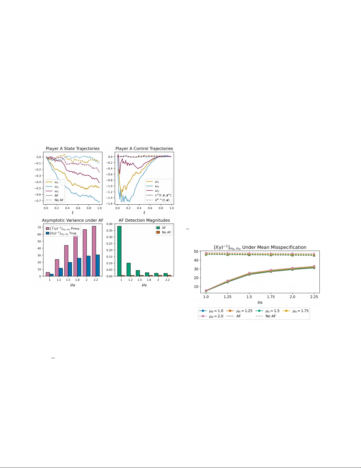
Inf ormation Rev elation and Alignment F aking in Stochastic Differ ential Games Daniel Ralston 1 , Xu Y ang 1 and Ruimeng Hu 1 , 2 Abstract — In competitive games with pri vate objectives, ac- tions can reveal inf ormation about hidden parameters. Quan- tifying such information r evelation, ho wever , is substantially more challenging, since it depends not only on the opponent’ s hidden parameter but also on the opponent’s model of the game. W e study this pr oblem via a two-player linear -quadratic stochastic differential game under partial information, in which each player knows its own coupling parameter and models the opponent’ s hidden parameter thr ough a prior . Starting from the full-information game, we characterize the Nash equilib- rium by coupled Riccati equations. W e then define baseline implementable controls by av eraging the equilibrium under each player’ s prior . Building on this baseline, we f ormulate an alignment-faking contr ol problem in which one play er trades off fidelity to its implementable policy against inf ormation acquisi- tion about the opponent’s hidden parameter . The information incentive is constructed from a proxy Fisher inf ormation matrix based only on the player’ s av ailable model. This leads to a tractable saddle-point formulation with semi-explicit control characterization through Riccati systems. Numerical illustra- tions show that alignment faking can substantially improve information gain ov er baseline play when the faker’ s model is accurate, but often at the cost of greater detectability . They also show that the proxy Fisher information can systematically differ from the true inf ormation under model misspecification. I . I N T RO D U C T I O N Information can be re vealed by actions in competitiv e games with pri v ate objecti ves. By observing an opponent’ s behavior , a player may infer features of its hidden objecti ve. Howe ver , quantifying such information revelation is non- trivial, since it depends not only on the opponent’ s priv ate objectiv e but also on the opponent’ s model of the game, a challenge described by T ownsend in [1] as “forecasting the forecasts of others. ” In games with priv ate information, a player must therefore reason through a proxy for the true information, constructed from its o wn av ailable quantities. This raises a further strategic question: Can a player delib- erately modify its behavior to rev eal more information about an opponent’ s hidden objective, while still appearing close to ordinary play? This paper addresses that question through what we call alignment faking (AF) contr ol . In our setting, AF refers to a control strategy that remains close to the This work was partially supported by the ONR grant #N00014-24-1-2432, the Simons Foundation (MP-TSM-00002783) and the NSF grant DMS- 2420988. 1 Department of Mathematics, University of California, Santa Barbara, CA 93106, USA. Email: { danielralston, xy6, rhu } @ucsb.edu . 2 Department of Statistics and Applied Probability , University of Califor- nia, Santa Barbara, CA 93106, USA. This work has been submitted to the IEEE for possible publication. Copyright may be transferred without notice, after which this version may no longer be accessible. Player A (AF) Public state: X A t , t ∈ [0 , T ] Hidden private parameter: m A Goal: track m A X B t Internal model: prior π B for m B Player B (Opponent) Public state: X B t , t ∈ [0 , T ] Hidden private parameter: m B Goal: track m B X A t Internal model: prior π A for m A AF control v ∗ Baseline implementable control u A, ∗ Baseline implementable control e u B , ∗ Observed trajectories X A t , X B t or Q1. Ho w does player A ’ s information about m B change depending on π A and π B ? Q2. Can the AF control yield trajectories that rev eal more information about m B ? Q3. Can player B detect the use of alignment faking v ∗ from observed trajectories? Fig. 1. Schematic of the alignment faking game. Each player kno ws its own coupling parameter and holds a prior on the opponent’s. Player A may deviate from the baseline implementable control via AF , while player B plays the baseline. player’ s baseline implementable control while intentionally steering the trajectory to extract more information about the opponent’ s hidden parameter . The term “alignment faking” is borrowed from the AI safety literature, where it refers to systems that strategically conceal their true objectives from overseers [2], [3]. Our model gi ves a continuous-time game-theoretic analogue: the player using the AF control plays the role of the AI system, while the opponent plays the role of the o verseer . Unlike much of the AI safety literature, where the objectiv e of AF is often left implicit, our framew ork makes the underlying tradeoff explicit through a control objective which balances information gain and closeness to baseline behavior . T o study this tradeoff, we consider a two-player linear- quadratic stochastic dif ferential game; see Figure 1 for a schematic illustration. W ithin this setting, we de velop an ana- lytically tractable quantitativ e framework that addresses how priv ate beliefs shape information rev elation, how purposeful deviations from baseline behavior affect information gain, and how such deviations may be detected. 1. Symmetric partial-information game with alignment faking: W e formulate a two-player continuous-time stochas- tic dif ferential game under partial information, extending earlier Stackelberg-type models [4] to a symmetric setting. W e deri ve implementable controls as expectations of the full- information Nash equilibrium under each player’ s prior on the opponent’ s hidden parameter . Building on this baseline, we introduce an additional information-seeking control ob- jectiv e defined through a proxy Fisher information matrix constructed from the player’ s a vailable quantities. W e obtain semi-explicit characterizations of the implementable and AF controls, and establish their well-posedness through coupled Riccati systems. 2. Numerical validation and discov ery: Numerical e x- periments sho w that the AF control can yield substantial information gains over baseline play when the alignment faker’ s model is well specified, b ut becomes more detectable. W e also sho w that the proxy Fisher information can sys- tematically misestimate the true information under model misspecification. Finally , we find that information quality depends mainly on the alignment faker’ s own model, while the opponent’ s model has a secondary but noticeable effect. Related Literatur e . Dynamic games hav e long been used to model strategic interactions among competing agents [5], [6], [7], [8], [9], [10]. Games with incomplete information, where parameters in the dynamics or cost functionals are not known to all players, are especially relev ant in adversarial settings arising in areas such as economics [11], cyber security [12], and, more recently , AI systems [3]. Previous works hav e studied Nash equilibria in linear-quadratic games with asymmetric information using the stochastic maximum principle [13] and with continuous type spaces via viscosity solutions of Hamilton–Jacobi equations [14]. In contrast, rather than solving for a full incomplete-information equi- librium, we model implementable controls by averaging the full-information Nash equilibrium under each player’ s prior , and then study how a player can strate gically deviate from this baseline to improve information extraction. Our work is also related to in verse learning and in verse optimal control, where the goal is to infer cost functions or unknown parameters from observed behavior [15], [16], [4], [17]. In the linear-quadratic setting, this in verse problem is closely tied to the coupled Riccati equations governing optimal controls, whose existence and solv ability hav e been widely studied [18], [19]. The ke y dif ference is that we do not study passi ve inference alone. Instead, we introduce an active control problem in which one player deliberately modifies its behavior to increase the information rev ealed by the trajectory . Notations. Boldface letters denote vectors. Super/subscripts A (resp. B ) index values associated with player A (resp. player B ), and the superscript AF indexes v alues associated with player A ’ s alignment faking problem. The operator diag {·} constructs a (block) diagonal matrix from its argu- ments. W e use ( · ) T for transpose, ∥ · ∥ F for the Frobenius norm, and S n × n for the space of n × n real symmetric matrices. An overline ( · ) and a tilde f ( · ) denotes quantities computed using player A ’ s and player B ’ s av ailable information (prior), while f ( · ) denotes a player A proxy for a player B quantity . I I . P RO B L E M S E T U P A N D B A S E L I N E N A S H E Q U I L I B R I U M This section formulates a stochastic differential game between two competing players, A and B . Assuming all model parameters are known to both players, we characterize the Nash equilibrium through a coupled Riccati system and provide conditions for its global existence. This full- information setting serves as a baseline for the partial- information case. A. State Dynamics and Cost Functionals Fix T > 0 and let (Ω , F , {F t } t ≥ 0 , P ) be a filtered probability space supporting a two-dimensional Brownian motion W t = [ W A t , W B t ] T . W e model players A and B by the R -v alued state processes X t = [ X A t , X B t ] T , controlled by u t = [ u A t , u B t ] T and subject to noise from W t , ev olving according to dX i t = u i t dt + σ i dW i t , i ∈ { A, B } , σ i > 0 . (1) Let m A , m B ∈ R be fixed parameters. Player i minimizes the cost functional J i [ u ] := E h Z T 0 f i ( t, x , u ; m i ) dt i , i ∈ { A, B } , (2) where the running cost of player i is quadratic, defined as f i ( t, x , u ; m i ) := q i ( x i − m i x − i ) 2 + r i ( u i ) 2 , with q i , r i > 0 , and − i refers to the player who is not i . For the baseline full-information game, we assume both players kno w both m A and m B , both dynamics (1), and cost functionals (2). The notion of interest is a Nash equilibrium (NE), namely , a pair of controls ( u A, ∗ , u B , ∗ ) such that neither player can reduce her cost by a unilateral deviation. In particular, we focus on Markovian NE of the form u i, ∗ t = u i, ∗ ( t, x ) , where u i, ∗ : [0 , T ] × R 2 → R is measurable for i ∈ { A, B } . B. Baseline Nash Equilibrium For i ∈ { A, B } , define the best-response value function V i ( t, x ) := inf u i E h Z T t f i ( s, X s , u s ; m i ) ds | X t = x i . By dynamic programming [6, Section 5.1.4], V A and V B satisfy a coupled HJB system 0 = ∂ t V A + inf u A u A ∂ x A V A + f A + u B , ∗ ∂ x B V A + σ 2 A 2 ∂ x A x A V A + σ 2 B 2 ∂ 2 x B x B V A , 0 = ∂ t V B + inf u B u B ∂ x B V B + f B + u A, ∗ ∂ x A V B + σ 2 A 2 ∂ x A x A V B + σ 2 B 2 ∂ 2 x B x B V B , with terminal conditions V i ( T , x ) = 0 , where u i, ∗ = inf u i { u i ∂ x i V i + f i } . Using the quadratic ansatz V i ( t, x ) = x T θ i ( t ) x + ψ i ( t ) , the NE takes the form u A, ∗ ( t, x ; m A , m B ) = − 1 r A x A θ A 11 ( t ) + x B θ A 12 ( t ) , (3) u B , ∗ ( t, x ; m A , m B ) = − 1 r B x A θ B 12 ( t ) + x B θ B 22 ( t ) . (4) Here, for each pair ( m A , m B ) , the matrices θ A ( t ) , θ B ( t ) ∈ S 2 × 2 solve the coupled Riccati system ˙ θ A ( t ) = θ A R A θ A + θ A R B θ B + θ B R B θ A − Q A , (5) ˙ θ B ( t ) = θ B R B θ B + θ A R A θ B + θ B R A θ A − Q B , (6) with terminal conditions θ A ( T ) = θ B ( T ) = 0 , where θ i j k ( t ) denotes the ( j, k ) -entry of θ i ( t ) , and Q A = q A − m A q A − m A q A m 2 A q A , R A = 1 r A 0 0 0 , Q B = m 2 B q B − m B q B − m B q B q B , R B = 0 0 0 1 r B . These equations follo w by substituting the ansatz into the coupled HJB system and matching coef ficients. Later, we sometimes put m A , m B after the semi-colon and write u i, ∗ ( t, x ; m A , m B ) and θ i ( t ; m A , m B ) , to emphasize the dependence on both parameters. Next, we state a proposition that will be important for the existence of implementable controls, discussed in Section III. Pr oposition 1: Let θ = diag { θ A , θ B } , and suppose T ≤ T ( m A , m B ) = ( c 1 c 2 ) − 1 / 2 · arctan (1 + m 2 A + m 2 B )( c 2 /c 1 ) − 1 / 2 , (7) where c 1 = 5( r − 2 A + r − 2 B ) 1 / 2 and c 2 = p q 2 A + q 2 B (1 + m 2 A + m 2 B ) . Then any solution to (5)–(6) on [0 , T ] satisfies θ ( t ; m A , m B ) F ≤ 1 + m 2 A + m 2 B . Pr oof: Write the coupled Riccati system in block form as ˙ θ = F ( θ ) − Q where Q := diag { Q A , Q B } , F ( θ ) := θ R A 0 0 R B θ + θ 0 R B R A 0 θ 0 I 2 I 2 0 + θ 0 R B R A 0 θ 0 I 2 I 2 0 T . By submultiplicati vity of the Frobenius norm, one has ∥ F ( θ ) ∥ F ≤ c 1 ∥ θ ∥ 2 F , ∥ Q ∥ F ≤ c 2 . Now define the time-rev ersed v ariable Y ( t ) := θ ( T − t ) . Then ˙ Y ( t ) = − F ( Y ( t )) + Q , and hence ∥ ˙ Y ( t ) ∥ F ≤ ∥ F ( Y ( t )) ∥ F + ∥ Q ∥ F ≤ c 1 ∥ Y ( t ) ∥ 2 F + c 2 . Consider the scalar ODE ˙ u = c 1 u 2 + c 2 , u (0) = 0 , with explicit solution u ( t ) = p c 2 /c 1 tan( √ c 1 c 2 t ) . It remains finite for t < π / (2 √ c 1 c 2 ) . Restricting t ≤ T ( m A , m B ) , we hav e u ( t ) ≤ (1 + m 2 A + m 2 B ) . Therefore, by [20, Corollary 6.3], ∥ Y ( T − t ) ∥ F ≤ u ( T − t ) , and the result follows. Pr oposition 2: Let T ≤ T ( m A , m B ) as in (7). Then the coupled Riccati system (5)–(6) for θ A , θ B admits a unique solution over [0 , T ] . Pr oof: Using the same definitions as in Proposition 1, let Y ( t ) = θ ( T − t ) so that Y solves the initial value problem ˙ Y = − F ( Y ) + Q , Y (0) = 0 . The right-hand side G ( Y ) := − F ( Y ) + Q is quadratic in Y , and is therefore locally Lipschitz on an y bounded subset of R 4 × 4 . By the Picard–Lindelhof theorem, there exists a unique solution of Y on [0 , T ∗ ) , where T ∗ is maximal. Suppose that T ∗ ≤ T ; then ∥ Y ( t ) ∥ F → ∞ as t → T ∗ . Howe ver , on [0 , T ∗ ) where the solution of Y ( t ) exists, Proposition 1 applies, yielding ∥ Y ( t ) ∥ F ≤ 1 + m 2 A + m 2 B for all t ∈ [0 , T ∗ − ϵ ] , contradicting blowup at T ∗ . I I I . G A M E U N D E R P A RT I A L I N F O R M A T I O N In the partial-information setting, the states and the cost functionals are fully kno wn to both players, b ut player A knows only m A and not the parameter m B in player B ’ s cost, while player B knows only m B and not m A . T o model this information structure, let M A ∈ [ m − A , m + A ] and M B ∈ [ m − B , m + B ] be random v ariables describing the players’ beliefs about m A and m B . Player A knows M A = m A and assigns a prior π B to M B , while player B kno ws M B = m B and assigns a prior π A to M A . The bounded supports ensure that the ODE bounds hold uniformly over all admissible realizations of M A and M B (cf. Proposition 1). Since the full-information NE controls (3)–(4) depend on both parameters, the y are generally not implementable in the partial-information setting. W e therefore introduce implementable controls, which depend only on each player’ s av ailable information, and deriv e their explicit forms. W e define implementable contr ols by taking expectations of the full-information NE controls under each player’ s prior: u A, ∗ ( t, x ; m A ) := E π B u A, ∗ ( t, x ; m A , M B ) , e u B , ∗ ( t, x ; m B ) := E π A u B , ∗ ( t, x ; M A , m B ) . The resulting controls are therefore u A, ∗ ( t, x ; m A ) = − 1 r A x A θ A 11 ( t ; m A ) + x B θ A 12 ( t ; m A ) , e u B , ∗ ( t, x ; m B ) = − 1 r B x A e θ B 12 ( t ; m B ) + x B e θ B 22 ( t ; m B ) , where θ i , e θ i , i ∈ { A, B } , are defined as θ A ( t ; m A ) := E π B θ A ( t ; m A , M B ) , e θ B ( t ; m B ) := E π A θ B ( t ; M A , m B ) , (8) and θ A ( t ; m A , M B ) , θ B ( t ; M A , m B ) are the matrix-valued solution of (5)–(6) corresponding to the parameter pair ( m A , M B ) and ( M A , m B ) ev aluated at time t . Note that θ A and e θ B are well defined by Proposition 1 and the compactness of [ m − A , m + A ] and [ m − B , m + B ] . Under the implementable controls, the state dynamics become dX A t = u A, ∗ ( t, X t ; m A ) dt + σ A dW A t , dX B t = e u B , ∗ ( t, X t ; m B ) dt + σ B dW B t . (9) Equiv alently , d X t = − θ A 11 ( t ; m A ) r A − θ A 12 ( t ; m A ) r A − e θ B 12 ( t ; m B ) r B − e θ B 22 ( t ; m B ) r B X t dt + Σ d W t , (10) with Σ := diag { σ A , σ B } . Since the drift is linear in X , with coefficients bounded on [0 , T ] , the system admits a unique strong solution. I V . A L I G N M E N T F A K I N G A N D I N F O R M A T I O N R E V E L A T I O N W e now formulate the alignment faking (AF) problem for player A . This choice is without loss of generality , and the same construction could be instead carried out for player B . The goal is for player A to choose a control that extracts information about player B ’ s hidden parameter m B , while also remaining close to the baseline implementable control u A, ∗ so as to reduce the risk that player B detects the deviation from the baseline play . Assumption 1 (T runcated Gaussian Priors): For the rest of the paper , we assume that both players model the op- ponent’ s unknown parameter by truncated Gaussians π A = N ( µ A , ρ 2 A ; m − A , m + A ) , π B = N µ B , ρ 2 B ; m − B , m + B , where N ( µ, ρ 2 ; a, b ) denotes a truncated Gaussian with density f ( m ; µ, ρ, a, b ) = ϕ m − µ ρ ρ Φ( b − µ ρ ) − Φ( a − µ ρ ) 1 [ a,b ] ( m ) , (11) and ϕ and Φ represent the density and cumulati ve distrib ution functions of a standard Gaussian N (0 , 1) . Under Assumption 1, player A kno ws m A and the prior parameters ( µ B , ρ B ) of π B , but does not know player B ’ s realized parameter m B nor player B ’ s prior parameters ( µ A , ρ A ) on m A . W e collect the quantities unknown to player A relev ant to player B ’ s control in γ := ( m B , µ A , ρ A ) . Let v t denote player A ’ s AF control, and let player B use the implementable control e u B , ∗ . The joint dynamics are d X t = b γ dt + Σ d W t , b γ := v t e u B , ∗ ( t, X t ; m B ) . (12) The objecti ve here will balance closeness to the baseline control (i.e. minimize ( v t − u A, ∗ t ) 2 ) with information acqui- sition about m B (cf. (14)). T o ensure v t is implementable, we impose the following assumption. Assumption 2: The AF control v t does not explicitly de- pend on the hidden quantities m B , µ A , or ρ A . Thus player A designs v t using only its available information, namely the realized parameter m A and the prior π B . In the sequel, we focus on implementable Marko vian AF controls for player A , namely controls of the form v t = v ( t, X t ; m A , π B ) , with E R T 0 | v t | 2 dt < ∞ . A. Likelihood Ratio and F isher Information (FI) T o quantify the information generated by player A ’ s control about γ , we deri ve its Fisher information matrix I ( γ ) . W e begin with the log-likelihood of γ based on the observed path { X t } 0 ≤ t ≤ T . Let P 0 be a reference measure under which X is driftless. By [21, Theorem 1.12], the log- likelihood is ℓ ( γ ) = Z T 0 b T γ (ΣΣ T ) − 1 d X t − 1 2 Z T 0 b T γ (ΣΣ T ) − 1 b γ dt. Differentiating with respect to γ j and using (12), we obtain ∂ γ j ℓ ( γ ) = R T 0 ( ∂ γ j b γ ) T (ΣΣ T ) − 1 Σ d W t . Hence the Fisher information matrix I ( γ ) has entries I ( γ ) j k = E h Z T 0 ( ∂ γ j b γ ) T (ΣΣ T ) − 1 ( ∂ γ k b γ ) dt i = 1 σ 2 B E h Z T 0 ∂ γ j e u B , ∗ t · ∂ γ k e u B , ∗ t dt i , where the second equality uses Assumption 2, as ∂ γ j v = 0 . The deriv ativ es ∂ γ e u B , ∗ are computed via differentiating the functions e θ B defined in (8). A direct calculation giv es ∂ µ A e θ B ( t ; m B ) = E π A [ θ B ( t ; M A , m B ) s µ A ( M A )] , ∂ ρ A e θ B ( t ; m B ) = E π A [ θ B ( t ; M A , m B ) s ρ A ( M A )] , (13) ∂ m B e θ B ( t ; m B ) = E π A [ ∂ m B θ B ( t ; M A , m B )] , where M A has density (11), ∂ m B θ B is obtained by dif ferenti- ating the Riccati system (5)–(6) with respect to m B , yielding linear ODEs with terminal conditions ∂ m B θ i ( T ) = 0 , and s µ A ( m ) = m − µ A ρ 2 A + ϕ m + A − µ A ρ A − ϕ m − A − µ A ρ A ρ A Φ m + A − µ A ρ A − Φ m − A − µ A ρ A , s ρ A ( m ) = ( m − µ A ) 2 ρ 3 A − 1 ρ A + m + A − µ A ρ A ϕ m + A − µ A ρ A − m − A − µ A ρ A ϕ m − A − µ A ρ A ρ A Φ m + A − µ A ρ A − Φ m − A − µ A ρ A . Remark 1 (FI and Information Revelation): Since player A seeks to re veal m B as much as possible, we use the asymp- totic variance of its maximum likelihood estimator (MLE) as a surrogate objective. Under regularity assumptions, if c M ( n ) B is an MLE estimator based on n independent repetitions of the game, then c M ( n ) B is consistent and asymptotically efficient: √ n c M ( n ) B − m B → N 0 , [ I ( γ ) − 1 ] m B ,m B . W e refer interested readers to [21, Theorem 2.8] or to [22, Theorem 5.1] for the finite dimensional case. Although we do not explicitly model a repeated-game estimation procedure, we use the asymptotic v ariance [ I ( γ ) − 1 ] m B ,m B as a surrogate for the information-gathering component of player A ’ s AF objective. T o characterize this quantity , we use Schur complement and write [ I ( γ ) − 1 ] m B ,m B = I m B ,m B − I m B , ( µ A ,ρ A ) ( I ( µ A ,ρ A ) , ( µ A ,ρ A ) ) − 1 I ( µ A ,ρ A ) ,m B − 1 , (14) with I ( µ A ,ρ A ) , ( µ A ,ρ A ) in vertible and I ( γ ) partitioned as I ( γ ) = I m B ,m B I m B , ( µ A ,ρ A ) I ( µ A ,ρ A ) ,m B I ( µ A ,ρ A ) , ( µ A ,ρ A ) . Moreov er , we observe that I m B ,m B − I m B , ( µ A ,ρ A ) ( I ( µ A ,ρ A ) , ( µ A ,ρ A ) ) − 1 I ( µ A ,ρ A ) ,m B = min z ∈ R 2 I m B ,m B + 2 z ⊤ I ( µ A ,ρ A ) ,m B + z ⊤ I ( µ A ,ρ A ) , ( µ A ,ρ A ) z . (15) This representation introduces an auxiliary variable z and av oids explicit products of Fisher-information entries, which is useful when constructing a quadratic AF objectiv e. B. Pr oxy Alignment F aking Objective The quantity [ I ( γ ) − 1 ] m B ,m B depends on parameters ( µ A , ρ A , m B ) which are unkno wn to player A , and cannot be optimized directly by player A. W e therefore construct a proxy objecti ve using only the quantities known to player A , namely ( m A , µ B , ρ B ) , yielding a max-min problem (16). T o motiv ate the proxy construction of [ I ( γ ) − 1 ] , suppose the truncation interval [ m − A , m + A ] is wide relativ e to ρ A , so that π A is close to the standard Gaussian N ( µ A , ρ 2 A ) . Writing M A ≈ µ A + ρ A Z with Z ∼ N (0 , 1) , the sensitivities in (13) may then be approximated by E Z ∂ m A θ B ( t ; µ A + ρ A Z, m B ) , E Z Z ∂ m A θ B ( t ; µ A + ρ A Z, m B ) , E Z ∂ m B θ B ( t ; µ A + ρ A Z, m B ) . Since player A does not kno w µ A and ρ A , we take this same approximate form b ut simply switch the randomness in arguments; we define pr oxy sensiti vities as ∂ µ A e θ B ( t ; m A ) := E Z ∂ m A θ B ( t ; m A , µ B + ρ B Z ) , ∂ ρ A e θ B ( t ; m A ) := E Z Z ∂ m A θ B ( t ; m A , µ B + ρ B Z ) , ∂ m B e θ B ( t ; m A ) := E π B [ ∂ m B θ B ( t ; m A , M B )] . where the last definition is for notational consistency . This can be understood as the worst case scenario of player A , in the sense that player B knows exactly her hidden parameter A and her prior π B on M B . Player A then uses ∂ γ e θ B as a pr oxy for ∂ γ e θ B . This yields the proxy Fisher information matrix I , whose j k -th entry is 1 σ 2 B r 2 B E h Z T 0 X A t ∂ γ j e θ B 12 + X B t ∂ γ j e θ B 22 · X A t ∂ γ k e θ B 12 + X B t ∂ γ k e θ B 22 dt i . As with I ( γ ) , we partition I as I = I m B ,m B I m B , ( µ A ,ρ A ) I ( µ A ,ρ A ) ,m B I ( µ A ,ρ A ) , ( µ A ,ρ A ) . Using the proxy I and the v ariational identity (15), we define the proxy AF cost functional J AF as J AF [ v , z ] := E h Z T 0 q AF ( v t − u A, ∗ t ) 2 + r AF v 2 t dt i − λ AF I m B ,m B +2 z T I ( µ A ,ρ A ) ,m B + z T I ( µ A ,ρ A ) , ( µ A ,ρ A ) z , where q AF , r AF > 0 penalize deviation from implementable baseline u A, ∗ t and control effort respectiv ely , while λ AF > 0 rewards information acquisition. W e then consider the saddle-point problem max z ∈ R 2 min v J AF [ v , z ] . (16) Importantly , player A optimizes J AF under dynamics d X t = v t , u B , ∗ t dt + Σ d W t , (17) where e u B , ∗ in (12) is replaced by u B , ∗ t := u B , ∗ ( t, X t ; m A ) with u B , ∗ ( t, x ; m A ) = E π B u B , ∗ ( t, x ; m A , M B ) since player A is unable to compute B ’ s true control e u B , ∗ . C. Solution via Quadratic Ansatz and Gradient Descent W e now solve the saddle-point problem (16)–(17). For z = [ z 1 , z 2 ] T , define the terms g 12 ( t, z ) := 1 r B z 1 ∂ µ A e θ B 12 + z 2 ∂ ρ A e θ B 12 + ∂ m B e θ B 12 , g 22 ( t, z ) := 1 r B z 1 ∂ µ A e θ B 22 + z 2 ∂ ρ A e θ B 22 + ∂ m B e θ B 22 . For fixed z ∈ R 2 , let V AF ( t, x ; z ) be the value function associated with J AF starting at X t = x . Using the HJB approach and a quadratic ansatz V AF ( t, x ; z ) = x T θ AF ( t ; z ) x + ψ AF ( t ; z ) , with θ AF ( t ) ∈ S 2 × 2 , the minimizer over v is given by v ∗ ( t, x ; z ) = − 1 q AF + r AF q AF r A x A θ A 11 ( t ) + x B θ A 12 ( t ) + x A θ AF 11 ( t ; z ) + x B θ AF 12 ( t ; z ) , (18) where θ AF ( t ; z ) solves the Riccati ODE ˙ θ AF = 1 q AF + r AF θ AF R A θ AF + q AF ( q AF + r AF ) r A θ AF R A θ A + θ A R A θ AF + θ AF R B θ B + θ B R B θ AF − q AF r AF ( q AF + r AF ) r 2 A θ A R A θ A − λ AF σ 2 B g 12 ( t, z ) g 22 ( t, z ) g 12 ( t, z ) g 22 ( t, z ) T , (19) with terminal condition θ AF ( T ) = 0 . Computing the saddle-point solution of (16) requires solv- ing (19) for each candidate z , simulating the corresponding controlled state paths, and optimizing over z . W e therefore propose an iterative scheme in Algorithm 1, which alternates between exact minimization in v through the Riccati ODEs and one gradient-ascent step in z using Monte Carlo esti- mates and automatic differentiation. Algorithm 1: Optimization of J AF Input: Initial value z (0) ∈ R 2 , conv ergence tolerance ϵ > 0 , learning rate α > 0 , sample size N MC ∈ N . Initialize k ← 0 , J AF prev ← −∞ , J AF curr ← ∞ ; while J AF curr − J AF prev > ϵ do Set J AF prev ← J AF curr ; Compute θ AF ( t ; z ( k ) ) ; Compute v ∗ ( t, x ; z ( k ) ) according to (18); Sample N MC paths of X A under v ∗ ( t, X t ; z ( k ) ) and X B under u B , ∗ ( t, X t ; m A ) ; Compute J AF curr ≈ J AF [ v ∗ ( · ; z ( k ) ) , z ( k ) ] with Monte Carlo; Compute ∇ z J AF curr ≈ ∇ z J AF [ v ∗ ( · ; z ( k ) ) , z ( k ) ] with automatic differentiation; Set z ( k +1) ← z ( k ) + α ∇ z J AF curr ; retur n z ∗ , v ∗ ( t, x ; z ∗ ) . Pr oposition 3 (Existence and Uniqueness of θ AF ): Let c A := max {| m − A | , | m + A |} , c B := max {| m − B | , | m + B |} , and assume ∥ z ∥ < r for some r > 0 . Define the constants c θ = max sup [0 , T ( c A ,c B )] ∥ θ A ∥ F , sup [0 , T ( c A ,c B )] ∥ θ B ∥ F , c g = sup [0 , T ( c A ,c B )] , ∥ z ∥
Original Paper
Loading high-quality paper...
Comments & Academic Discussion
Loading comments...
Leave a Comment