Asymmetric Nash Seeking via Best Response Maps: Global Linear Convergence and Robustness to Inexact Reaction Models

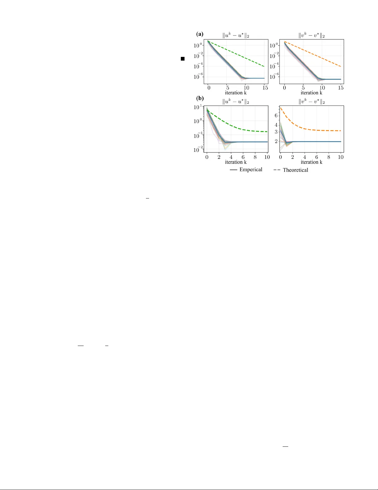
Asymmetric Nash Seeking via Best–Response Maps: Global Linear Con ver gence and Rob ustness to Inexact Reaction Models Mahdis Rabbani 1 , Navid Mojahed 1 , and Shima Nazari 1 Abstract — Nash equilibria pro vide a principled framework for modeling interactions in multi-agent decision-making and control. Howev er , many equilibrium-seeking methods implicitly assume that each agent has access to the other agents’ objectives and constraints, an assumption that is often unrealistic in practice. This letter studies a class of asymmetric-inf ormation two-player constrained games with decoupled feasible sets, in which Player 1 knows its o wn objective and constraints while Player 2 is av ailable only through a best-response map. For this class of games, we propose an asymmetric projected gradient descent–best response iteration that does not requir e full mutual knowledge of both players’ optimization problems. Under suitable regularity conditions, we establish existence and uniqueness of the Nash equilibrium and prov e global linear con vergence of the proposed iteration when the best-response map is exact. Recognizing that best-response maps are often learned or estimated, we further analyze the inexact case and show that, when the approximation error is uniformly bounded by ε , the iterates enter an explicit O ( ε ) neighborhood of the true Nash equilibrium. Numerical results on a benchmark game corr oborate the predicted con vergence behavior and error scaling. I . I N T RO D U C T I O N Strategic decision-making in multi-agent systems is central to autonomy , robotics, and networked control, where agents pursue indi vidual objecti ves while influencing one another through coupled decisions and shared en vironments [1]–[4]. In such settings, Nash equilibrium (NE) provides a principled notion of interaction-consistent behavior and underlies a broad class of game-theoretic planning and control methods [3]–[5]. This viewpoint is especially appealing in interaction- aware autonomy , where mutual adaptation arises naturally in scenarios such as lane changes, mer ges, overtaking, and human–robot interaction [3], [4], [6], [7]. A central limitation of many equilibrium-based methods is their information assumption. Classical equilibrium analysis and computation typically assume that the game is explicitly known, including all players’ objecti ves and feasible sets [5], [8]–[10]. This assumption is b uilt into both foundational theory and practical game solvers, including VI/KKT -based approaches and modern constrained dynamic-game solvers such as ALGAMES and DG-SQP [6], [8], [9], [11]. A complementary fixed-point vie wpoint leads to iterati ve best- response (IBR) schemes and related Jacobi/Gauss–Seidel updates [3], [12], [13]. Ho we ver , both perspecti ves still rely on access to either the full joint game model or repeatedly ev aluable opponent best responses, which is restrictive in 1 Authors are with Department of Mechanical and Aerospace Engineer- ing, University of California, Davis, One Shield A ve, Davis, CA 95616. { mrabbani, nmojahed, snazari } @ucdavis.edu interactiv e settings where surrounding agents are observed only through beha vior rather than through their internal optimization problems [12], [14]. T o address this asymmetry , recent efforts hav e sought to recover missing opponent information from data, for example by learning latent objectiv es or adapting opponent models online [14]–[16]. In contrast, we study a class of asymmetric-information two-player constrained games with decoupled feasible sets, in which Player 1 kno ws its o wn objectiv e and constraints, while Player 2 is represented only through a best-response map [17]. Thus, Player 2’ s objectiv e, model, and constraints need not be explicitly accessible. Importantly , the best-response map is treated here as an information structur e , not as a leader–follo wer reformulation; our goal is to characterize and seek the simultaneous-move Nash equilibrium of the original game under asymmetric information, rather than a Stackelberg solution [7], [18]. The main contributions of this paper are as follo ws: • W e introduce a class of asymmetric-information two- player constrained games with decoupled feasible sets, in which the opponent is represented directly through a best-response map rather than an explicit objecti ve model, and establish existence and uniqueness of Nash equilibrium for this class under regularity assumptions. • W e propose an asymmetric projected gradient descent– best response iteration and show that, under stronger regularity assumptions, it con verges globally and lin- early to the unique Nash equilibrium. • W e analyze the practically important case of an approx- imate best-response map and prov e rob ustness: under a uniform approximation error bound, the proposed iteration enters an e xplicit O ( ε ) neighborhood of the true Nash equilibrium. T ak en together , these results turn the best-response-map viewpoint from a modeling abstraction into a prov ably con vergent equilibrium-seeking frame work for constrained games with asymmetric information. I I . P RO B L E M F O R M U L A T I O N W e consider a constrained two-player game with decision variables x 1 ∈ X 1 ⊂ R n 1 and x 2 ∈ X 2 ⊂ R n 2 for Player 1 and Player 2, respectiv ely . The feasible sets are decoupled, so the joint feasible set is X ≜ X 1 × X 2 , and there is no explicit coupling through shared constraints. Thus, the interaction enters through the cost functions and the induced reaction beha vior rather than through joint feasibility conditions. Player 1 is described by a cost function J 1 : X 1 × X 2 → R , ( x 1 , x 2 ) 7→ J 1 ( x 1 , x 2 ) , (1) which may depend on both players’ decisions. In contrast, Player 2 is represented, from the standpoint of Player 1, through its best-response correspondence BR 2 : X 1 ⇒ X 2 , BR 2 ( x 1 ) ≜ arg min x 2 ∈ X 2 J 2 ( x 1 , x 2 ) , (2) for some objectiv e J 2 that need not be known to Player 1. Accordingly , the algorithmic de velopment relies only on access to BR 2 ( · ) , or later , an approximation thereof. Pr oblem 1 (Asymmetric-Information T wo-Player Game): Giv en the feasible sets X 1 , X 2 , Player 1’ s cost J 1 in (1), and Player 2’ s best-response correspondence BR 2 ( · ) in (2), consider the two-player game in which Player 1 solves min x 1 ∈ X 1 J 1 ( x 1 , x 2 ) , while Player 2 simultaneously reacts according to x 2 ∈ BR 2 ( x 1 ) . Definition 1 (Nash equilibrium): A pair ( x ⋆ 1 , x ⋆ 2 ) ∈ X 1 × X 2 is a Nash equilibrium of Problem 1 if x ⋆ 1 ∈ arg min x 1 ∈ X 1 J 1 ( x 1 , x ⋆ 2 ) , x ⋆ 2 ∈ BR 2 ( x ⋆ 1 ) . The next section characterizes conditions under which Problem 1 admits a Nash equilibrium and when that equi- librium is unique. I I I . E X I S T E N C E & U N I Q U E N E S S O F T H E E Q U I L I B R I U M This section inv estigates e xistence and uniqueness of a Nash equilibrium for Problem 1. W e first establish existence under general re gularity conditions that allo w Player 2’ s best- response map to be set-valued, and then impose stronger assumptions under which the best response becomes single- valued and the equilibrium is unique. Assumption A.1: The feasible sets X 1 and X 2 are nonempty , conv ex, and compact. Assumption A.2: The function J 1 : X 1 × X 2 → R is continuous on X 1 × X 2 . Moreover , for e very fixed x 2 ∈ X 2 , the function J 1 ( · , x 2 ) is con vex on X 1 . Assumption A.3: For ev ery x 1 ∈ X 1 , the correspondence BR 2 ( x 1 ) ⊆ X 2 is nonempty , con vex, and compact, and BR 2 : X 1 ⇒ X 2 is upper hemicontinuous. Theor em 1 (Existence of Nash equilibrium): Under Assumptions A.1–A.3, Problem 1 admits at least one Nash equilibrium. Pr oof: Define Player 1’ s best-response correspondence BR 1 ( x 2 ) ≜ arg min x 1 ∈ X 1 J 1 ( x 1 , x 2 ) , x 2 ∈ X 2 . (3) Fix any x 2 ∈ X 2 . By Assumption A.1, X 1 is nonempty and compact, and by Assumption A.2, J 1 ( · , x 2 ) is contin- uous. Hence, by the W eierstrass extreme value theorem, BR 1 ( x 2 ) is nonempty and compact. Moreover , by conv ex- ity of J 1 ( · , x 2 ) (Assumption A.2), the set of minimizers BR 1 ( x 2 ) is con vex. Next, Assumption A.2 ensures that J 1 is jointly continuous on X 1 × X 2 , while Assumption A.1 guarantees that X 1 is compact. Therefore, Berge’ s maximum theorem implies that BR 1 : X 2 ⇒ X 1 is upper hemicontinuous and compact- valued. Now define the product correspondence F : X ⇒ X on X = X 1 × X 2 by F ( x 1 , x 2 ) ≜ BR 1 ( x 2 ) × BR 2 ( x 1 ) . By the preceding arguments and Assumption A.3, for ev- ery ( x 1 , x 2 ) ∈ X the set F ( x 1 , x 2 ) is nonempty , con vex, and compact, and F is upper hemicontinuous. Since X is nonempty , conv ex, and compact by Assumption A.1, Kakutani’ s fixed-point theorem guarantees the existence of ( x ⋆ 1 , x ⋆ 2 ) ∈ X such that ( x ⋆ 1 , x ⋆ 2 ) ∈ F ( x ⋆ 1 , x ⋆ 2 ) , i.e., x ⋆ 1 ∈ BR 1 ( x ⋆ 2 ) and x ⋆ 2 ∈ BR 2 ( x ⋆ 1 ) . By the definition of BR 1 in (3), the first inclusion is equi v alent to x ⋆ 1 ∈ arg min x 1 ∈ X 1 J 1 ( x 1 , x ⋆ 2 ) , and together with x ⋆ 2 ∈ BR 2 ( x ⋆ 1 ) this matches Definition 1. Therefore, ( x ⋆ 1 , x ⋆ 2 ) is a Nash equilibrium of Problem 1. T o state a uniqueness condition aligned with our sub- sequent con vergence analysis, we impose the follo wing stronger assumptions. Assumption B.1: The function J 1 : X 1 × X 2 → R is continuous on X 1 × X 2 . Moreover , for e very fixed x 2 ∈ X 2 , the function J 1 ( · , x 2 ) is differentiable and µ -strongly con ve x on X 1 for some µ > 0 . Assumption B.2: For every fixed x 1 ∈ X 1 , the mapping x 2 7→ ∇ x 1 J 1 ( x 1 , x 2 ) is Lipschitz on X 2 with constant L 12 ≥ 0 , i.e., ∀ x 2 , y 2 ∈ X 2 , ∥∇ x 1 J 1 ( x 1 , x 2 ) − ∇ x 1 J 1 ( x 1 , y 2 ) ∥ ≤ L 12 ∥ x 2 − y 2 ∥ . Assumption B.3: For e very x 1 ∈ X 1 , the best response map BR 2 ( x 1 ) is single-v alued. Assumption B.4: The (single-valued) best response map BR 2 : X 1 → X 2 is Lipschitz on X 1 with constant L 2 ≥ 0 . Theor em 2 (Uniqueness of Nash equilibrium): Suppose Assumptions A.1 and B.1 – B.4 hold. If µ > L 12 L 2 , then the Nash equilibrium of Problem 1 is unique. Pr oof: Assumption B.1 implies Assumption A.2. In addition, Assumptions B.3 and B.4 imply that BR 2 is a continuous single-valued map, hence upper hemicontinuous as a correspondence with nonempty , con ve x, and compact singleton values. Therefore, Assumption A.3 also holds. T ogether with Assumption A.1, existence follows from The- orem 1. T o prove uniqueness, let ( a 1 , b 1 ) and ( a 2 , b 2 ) be two Nash equilibria of Problem 1. By Definition 1 and Assumption B.3, b 1 = BR 2 ( a 1 ) , b 2 = BR 2 ( a 2 ) . (4) Since a 1 minimizes J 1 ( · , b 1 ) ov er the conv ex set X 1 , the first- order optimality condition for con vex constrained problems yields ⟨∇ x 1 J 1 ( a 1 , b 1 ) , a 2 − a 1 ⟩ ≥ 0 . Similarly , optimality of a 2 for J 1 ( · , b 2 ) implies ⟨∇ x 1 J 1 ( a 2 , b 2 ) , a 1 − a 2 ⟩ ≥ 0 . Adding the two inequalities gives ⟨∇ x 1 J 1 ( a 1 , b 1 ) − ∇ x 1 J 1 ( a 2 , b 2 ) , a 1 − a 2 ⟩ ≤ 0 . (5) Add and subtract ∇ x 1 J 1 ( a 2 , b 1 ) inside the inner product in (5). By µ -strong con vexity of J 1 ( · , b 1 ) (Assumption B.1), we hav e ⟨∇ x 1 J 1 ( a 1 , b 1 ) − ∇ x 1 J 1 ( a 2 , b 1 ) , a 1 − a 2 ⟩ ≥ µ ∥ a 1 − a 2 ∥ 2 . (6) For the remaining term, Cauchy–Schwarz yields ⟨∇ x 1 J 1 ( a 2 , b 1 ) − ∇ x 1 J 1 ( a 2 , b 2 ) , a 1 − a 2 ⟩ ≥ −∥∇ x 1 J 1 ( a 2 , b 1 ) − ∇ x 1 J 1 ( a 2 , b 2 ) ∥ ∥ a 1 − a 2 ∥ . Using Assumption B.2 and (4) together with Assump- tion B.4, we obtain ⟨∇ x 1 J 1 ( a 2 , b 1 ) − ∇ x 1 J 1 ( a 2 , b 2 ) , a 1 − a 2 ⟩ ≥ − L 12 ∥ b 1 − b 2 ∥ ∥ a 1 − a 2 ∥ ≥ − L 12 L 2 ∥ a 1 − a 2 ∥ 2 . (7) Combining (5)–(7) yields ( µ − L 12 L 2 ) ∥ a 1 − a 2 ∥ 2 ≤ 0 . If µ > L 12 L 2 , then a 1 = a 2 . Substituting into (4), and gi ven Assumption B.3, gi ves b 1 = b 2 , hence ( a 1 , b 1 ) = ( a 2 , b 2 ) . Therefore, the Nash equilibrium is unique. The same dominance condition µ > L 12 L 2 also induces a monotonicity mar gin that will be central to the con vergence analysis of the iterati ve scheme developed next. I V . A L G O R I T H M & G L O B A L L I N E A R C O N V E R G E N C E T O T H E E Q U I L I B R I U M Under Assumptions A.1 and B.1 – B.4, and whenever µ > L 12 L 2 , Problem 1 admits a unique Nash equilibrium by Theorem 2. W e now study a projected best-response/gradient iteration and sho w that it con ver ges globally and linearly to this equilibrium. Assumption C.1: For e very fixed x 2 ∈ X 2 , the function J 1 ( · , x 2 ) is L 1 -smooth on X 1 , i.e., ∀ x 1 , y 1 ∈ X 1 , ∥∇ x 1 J 1 ( x 1 , x 2 ) − ∇ x 1 J 1 ( y 1 , x 2 ) ∥ ≤ L 1 ∥ x 1 − y 1 ∥ . W e consider the projected best-response/gradient iteration x k 2 = BR 2 ( x k 1 ) , x k +1 1 = Π X 1  x k 1 − α ∇ x 1 J 1 ( x k 1 , x k 2 )  , (8) where Π X 1 ( · ) denotes the Euclidean projection onto X 1 . Since X 1 is closed and con vex (Assumption A.1), the pro- jection is nonexpansi ve: ∥ Π X 1 ( u ) − Π X 1 ( v ) ∥ ≤ ∥ u − v ∥ , ∀ u, v ∈ R n 1 . (9) Theor em 3 (Global linear conver gence): Suppose Assumptions A.1, B.1 – B.4, and C.1 hold. Let m ≜ µ − L 12 L 2 and L G ≜ L 1 + L 12 L 2 , and note that m > 0 follows from µ > L 12 L 2 . Then, for any stepsize α satisfying 0 < α < 2 m L 2 G = 2( µ − L 12 L 2 ) ( L 1 + L 12 L 2 ) 2 , the iterates generated by (8) satisfy ∥ x k 1 − x ⋆ 1 ∥ ≤ ρ ( α ) k ∥ x 0 1 − x ⋆ 1 ∥ , ∥ x k 2 − x ⋆ 2 ∥ ≤ L 2 ρ ( α ) k ∥ x 0 1 − x ⋆ 1 ∥ , where ( x ⋆ 1 , x ⋆ 2 ) is the unique Nash equilibrium of Problem 1 and ρ ( α ) ≜ q 1 − 2 αm + α 2 L 2 G ∈ (0 , 1) . Pr oof: Define the map T : X 1 → X 1 by T ( x 1 ) := Π X 1  x 1 − α ∇ x 1 J 1  x 1 , BR 2 ( x 1 )  , (10) and define the operator G : X 1 → R n 1 as G ( x 1 ) := ∇ x 1 J 1  x 1 , BR 2 ( x 1 )  . For any x 1 , y 1 ∈ X 1 , add and subtract ∇ x 1 J 1 ( y 1 , BR 2 ( x 1 )) to obtain ∥ G ( x 1 ) − G ( y 1 ) ∥ ≤ ∥∇ x 1 J 1 ( x 1 , BR 2 ( x 1 )) − ∇ x 1 J 1 ( y 1 , BR 2 ( x 1 )) ∥ + ∥∇ x 1 J 1 ( y 1 , BR 2 ( x 1 )) − ∇ x 1 J 1 ( y 1 , BR 2 ( y 1 )) ∥ . By Assumption C.1, the first term is bounded by L 1 ∥ x 1 − y 1 ∥ . By Assumptions B.2 and B.4, the second term is bounded by L 12 ∥ BR 2 ( x 1 ) − BR 2 ( y 1 ) ∥ ≤ L 12 L 2 ∥ x 1 − y 1 ∥ . Therefore, G is Lipschitz on X 1 with constant L G = L 1 + L 12 L 2 , i.e., ∥ G ( x 1 ) − G ( y 1 ) ∥ ≤ L G ∥ x 1 − y 1 ∥ . (11) Next, using the same add–subtract decomposition and Assumption B.1, we ha ve ⟨ G ( x 1 ) − G ( y 1 ) , x 1 − y 1 ⟩ = ⟨∇ x 1 J 1 ( x 1 , BR 2 ( x 1 )) − ∇ x 1 J 1 ( y 1 , BR 2 ( x 1 )) , x 1 − y 1 ⟩ + ⟨∇ x 1 J 1 ( y 1 , BR 2 ( x 1 )) − ∇ x 1 J 1 ( y 1 , BR 2 ( y 1 )) , x 1 − y 1 ⟩ . The first inner product is lower bounded by µ ∥ x 1 − y 1 ∥ 2 . For the second, Cauchy–Schwarz together with Assumptions B.2 and B.4 yields ⟨∇ x 1 J 1 ( y 1 , BR 2 ( x 1 )) − ∇ x 1 J 1 ( y 1 , BR 2 ( y 1 )) , x 1 − y 1 ⟩ ≥ − L 12 L 2 ∥ x 1 − y 1 ∥ 2 . Thus, G is strongly monotone on X 1 with constant m = µ − L 12 L 2 > 0 , i.e., ⟨ G ( x 1 ) − G ( y 1 ) , x 1 − y 1 ⟩ ≥ m ∥ x 1 − y 1 ∥ 2 . (12) By nonexpansi veness of the projection (9), ∥ T ( x 1 ) − T ( y 1 ) ∥ ≤ ∥ ( x 1 − y 1 ) − α ( G ( x 1 ) − G ( y 1 )) ∥ . Expanding the square and applying the Lipschitz and strong monotonicity bounds in (11) and (12) gives ∥ T ( x 1 ) − T ( y 1 ) ∥ 2 ≤  1 − 2 αm + α 2 L 2 G  ∥ x 1 − y 1 ∥ 2 =: q ( α ) ∥ x 1 − y 1 ∥ 2 . (13) For 0 < α < 2 m/L 2 G , we ha ve q ( α ) ∈ (0 , 1) , hence T is a contraction with modulus ρ ( α ) = p q ( α ) ∈ (0 , 1) . Therefore, by the Banach fix ed-point theorem, T has a unique fixed point x ∗ 1 ∈ X 1 and the iterates satisfy ∥ x k 1 − x ∗ 1 ∥ ≤ ρ ( α ) k ∥ x 0 1 − x ∗ 1 ∥ . (14) Let x ∗ 2 := BR 2 ( x ∗ 1 ) . Since BR 2 is Lipschitz (B.4),   x k 2 − x ∗ 2   =   BR 2 ( x k 1 ) − BR 2 ( x ∗ 1 )   ≤ L 2   x k 1 − x ∗ 1   . Combining with (14) gi ves   x k 2 − x ∗ 2   ≤ L 2 ρ ( α ) k   x 0 1 − x ∗ 1   . It remains to show that x ∗ 1 minimizes J 1 ( · , x ∗ 2 ) ov er X 1 . From x ∗ 1 = T ( x ∗ 1 ) , we ha ve x ∗ 1 = Π X 1 ( x ∗ 1 − α ∇ x 1 J 1 ( x ∗ 1 , x ∗ 2 )) . By the characterization of Euclidean projection onto a closed con vex set, y = Π X 1 ( z ) if and only if ⟨ z − y , x − y ⟩ ≤ 0 , ∀ x ∈ X 1 . Applying this with y = x ∗ 1 and z = x ∗ 1 − α ∇ x 1 J 1 ( x ∗ 1 , x ∗ 2 ) yields ⟨∇ x 1 J 1 ( x ∗ 1 , x ∗ 2 ) , x − x ∗ 1 ⟩ ≥ 0 , ∀ x ∈ X 1 . Since J 1 ( · , x ∗ 2 ) is con ve x and differentiable (B.1), this first- order condition is suf ficient for optimality , hence x ∗ 1 ∈ arg min x 1 ∈ X 1 J 1 ( x 1 , x ∗ 2 ) . T ogether with x ∗ 2 = BR 2 ( x ∗ 1 ) , Definition 1 implies that ( x ∗ 1 , x ∗ 2 ) is a Nash equilibrium. By uniqueness (Theorem 2), ( x ∗ 1 , x ∗ 2 ) = ( x ⋆ 1 , x ⋆ 2 ) , which completes the proof. V . I N E X AC T B E S T R E S P O N S E & R O B U S T N E S S O F T H E A L G O R I T H M The con ver gence result in Section IV assumes access to the exact best-response map BR 2 . In practice, howe ver , an agent typically has access only to an approximation or estimate of its opponent’ s reaction behavior . W e therefore study the robustness of the projected best-response/gradient iteration when BR 2 is replaced by an ine xact map. Let d BR 2 : X 1 → X 2 denote an approximation of BR 2 , and assume a uniform error bound: there exists ε > 0 such that ∥ d BR 2 ( x 1 ) − BR 2 ( x 1 ) ∥ ≤ ε, ∀ x 1 ∈ X 1 . (15) W e consider the inexact variant of (8): x k 2 = d BR 2 ( x k 1 ) , x k +1 1 = Π X 1  x k 1 − α ∇ x 1 J 1 ( x k 1 , x k 2 )  . (16) Theor em 4 (Rob ustness to ine xact best r esponse): Let ( x ⋆ 1 , x ⋆ 2 ) ∈ X denote the unique Nash equilibrium of Problem 1 under Assumptions A.1, B.1 – B.4, and C.1, and suppose µ > L 12 L 2 . Let m ≜ µ − L 12 L 2 , L G ≜ L 1 + L 12 L 2 , and choose α ∈ (0 , 2 m/L 2 G ) . If d BR 2 satisfies (15), then the iterates (16) satisfy , for all k ≥ 0 , ∥ x k +1 1 − x ⋆ 1 ∥ ≤ ρ ( α ) ∥ x k 1 − x ⋆ 1 ∥ + αL 12 ε, (17) where ρ ( α ) = q 1 − 2 αm + α 2 L 2 G ∈ (0 , 1) . Consequently , lim sup k →∞ ∥ x k 1 − x ⋆ 1 ∥ ≤ αL 12 1 − ρ ( α ) ε. (18) Moreov er , the sequence x k 2 = d BR 2 ( x k 1 ) satisfies ∥ x k 2 − x ⋆ 2 ∥ ≤ L 2 ∥ x k 1 − x ⋆ 1 ∥ + ε, (19) and hence lim sup k →∞ ∥ x k 2 − x ⋆ 2 ∥ ≤  L 2 αL 12 1 − ρ ( α ) + 1  ε. (20) Pr oof: Let T : X 1 → X 1 denote the exact map from (10) and define the ine xact map b T : X 1 → X 1 by b T ( x 1 ) := Π X 1  x 1 − α ∇ x 1 J 1  x 1 , d BR 2 ( x 1 )   . By Theorem 3, T is a contraction on X 1 with modulus ρ ( α ) ∈ (0 , 1) , i.e. (13). Moreover , using nonexpansi veness of the projection (9), Assumption B.2, and (15), we obtain, for any x 1 ∈ X 1 , ∥ b T ( x 1 ) − T ( x 1 ) ∥ ≤ α    ∇ x 1 J 1  x 1 , d BR 2 ( x 1 )  − ∇ x 1 J 1  x 1 , BR 2 ( x 1 )     ≤ αL 12 ∥ d BR 2 ( x 1 ) − BR 2 ( x 1 ) ∥ ≤ αL 12 ε. (21) Now , since x k +1 1 = b T ( x k 1 ) and x ⋆ 1 = T ( x ⋆ 1 ) , we ha ve ∥ x k +1 1 − x ⋆ 1 ∥ = ∥ b T ( x k 1 ) − T ( x ⋆ 1 ) ∥ ≤ ∥ b T ( x k 1 ) − T ( x k 1 ) ∥ + ∥ T ( x k 1 ) − T ( x ⋆ 1 ) ∥ . Using the contraction property of T from Theorem 3 together with (21), immediately prov es (17). Iterating (17) yields ∥ x k 1 − x ⋆ 1 ∥ ≤ ρ ( α ) k ∥ x 0 1 − x ⋆ 1 ∥ + αL 12 ε k − 1 X i =0 ρ ( α ) i . Since ρ ( α ) ∈ (0 , 1) , k − 1 X i =0 ρ ( α ) i = 1 − ρ ( α ) k 1 − ρ ( α ) , and therefore, for all k ≥ 0 , ∥ x k 1 − x ⋆ 1 ∥ ≤ ρ ( α ) k ∥ x 0 1 − x ⋆ 1 ∥ + 1 − ρ ( α ) k 1 − ρ ( α ) αL 12 ε. T aking lim sup as k → ∞ giv es (18). Finally , since x k 2 = d BR 2 ( x k 1 ) and x ⋆ 2 = BR 2 ( x ⋆ 1 ) , we write ∥ x k 2 − x ⋆ 2 ∥ = ∥ d BR 2 ( x k 1 ) − BR 2 ( x ⋆ 1 ) ∥ ≤ ∥ d BR 2 ( x k 1 ) − BR 2 ( x k 1 ) ∥ + ∥ BR 2 ( x k 1 ) − BR 2 ( x ⋆ 1 ) ∥ . The first term is bounded by ε via (15), and the second is bounded by L 2 ∥ x k 1 − x ⋆ 1 ∥ via Assumption B.4, proving (19). Combining (19) with (18) yields (20) and concludes the proof. Theorem 4 shows that under a uniform approximation error in the opponent’ s best-response map, the projected best-response/gradient iteration remains practically stable: the Player 1 iterate ultimately enters an O ( ε ) neighborhood of the e xact Nash equilibrium, and the resulting Player 2 estimate remains within an O ( ε ) neighborhood of x ⋆ 2 as well. If, in addition, d BR 2 is single-valued and Lipschitz on X 1 with constant b L 2 such that µ > L 12 b L 2 , then the same contraction argument as in Theorem 3 applies with BR 2 replaced by d BR 2 , implying linear con vergence of (16) to the unique equilibrium of the perturbed game induced by d BR 2 . V I . N U M E R I C A L E X A M P L E W e illustrate the theoretical results on a one-dimensional tug-of-war cart in which two agents apply opposing longi- tudinal forces to a point mass with viscous drag. Player 1 selects an open-loop control sequence u , while Player 2 reacts through a best-response map. The example is designed to instantiate the assumptions of Theorems 1 – 4 and to illus- trate exact con ver gence, robustness to inexact best-response information, and the predicted O ( ε ) neighborhood scaling. Let z t = [ p t , ˙ p t ] ⊤ ∈ R 2 denote position and velocity of the cart at time step t . With sampling time ∆ t , mass m , and viscous drag coef ficient b , the discrete-time dynamics are z t +1 = A d z t + B u u t + B v v t , t = 0 , . . . , N − 1 , where z 0 = [0 , 0] ⊤ and A d =  1 ∆ t 0 1 − ∆ t ( b/m )  , B u = − B v =  0 ∆ t/m  . Stacking the horizon v ariables as u = [ u 0 , . . . , u N − 1 ] ⊤ , v = [ v 0 , . . . , v N − 1 ] ⊤ , results in the predicted state trajectory of the affine form Z ( u, v ) = S 0 + S u u + S v v . Player 1 selects u ∈ X 1 to minimize J 1 ( u, v ) = q u 2 ∥ u ∥ 2 2 + 1 2 Z ( u, v ) ⊤ QZ ( u, v ) − r pull C ⊤ x Z ( u, v ) + γ u ⊤ v , where Q = blkdiag( q pos , q vel , . . . , q pos , q vel ) ⪰ 0 penalizes predicted states, and C x selects position components so that C ⊤ x Z ( u, v ) = P N t =1 p t . The feasible set of Player 1 is the box X 1 := { u ∈ R N | u min ≤ u t ≤ u max , t = 0 , . . . , N − 1 } . Player 2 is modeled through a stage wise best-response map BR 2 ( u ) = v max tanh  κ ( v bar + c react u )  , which captures a saturating reaction. Consistent with the asymmetric-information formulation of Problem 1, Player 2 Fig. 1. Conv ergence under e xact and inexact best responses. (a) exact best response gives linear con vergence from multiple initializations; (b) inexact best response yields conv ergence to an ε -dependent neighborhood. is specified here only through its reaction map BR 2 ( · ) ; an explicit objecti ve model J 2 is not required for the example. Since | BR 2 ( u ) t | ≤ v max , we take X 2 := { v ∈ R N | ∥ v ∥ ∞ ≤ v max } . The constants ( µ, L 1 , L 12 , L 2 ) are computed analytically from the quadratic cost and the slope bounds of the reaction map using eigen value and spectral-norm bounds; in particu- lar , µ and L 1 come from the Hessian with respect to u . W e use N = 5 , | u | ≤ 3 , (∆ t, m, b ) = (0 . 2 , 1 . 0 , 0 . 6) , ( q u , q pos , q vel ) = (0 . 35 , 0 . 32 , 0 . 01) , ( r pull , γ ) = (5 . 4 , 0 . 01) , and ( v max , κ, v bar , c react ) = (1 . 8 , 0 . 6 , 0 . 9 , 0 . 9) . These yield µ = 0 . 3502 , L 1 = 0 . 3725 , L 12 = 0 . 0125 , L 2 = 0 . 9720 , so µ > L 12 L 2 holds and the Nash equilibrium is unique by Theorem 2. The corresponding stepsize limit is α max = 4 . 57 . W e first consider the exact iteration (8) with α = 0 . 5 α max , which gives ρ ( α ) = 0 . 48 < 1 . Fig. 1(a) sho ws ∥ u k − u ⋆ ∥ 2 and ∥ v k − v ⋆ ∥ 2 from multiple random initializations, together with the theoretical decay references from Theorem 3. A reference equilibrium ( u ⋆ , v ⋆ ) is computed by iterating the exact map to a tight tolerance. The observ ed trajectories exhibit the predicted linear con vergence, while the late-stage flattening is due to numerical tolerance. T o model limited access to BR 2 ( · ) , we approximate the scalar map b ( u ) = v max tanh  κ ( v bar + c react u )  by its first- order T aylor expansion about u = 0 , b b ( u ) = v max tanh( κv bar ) +  v max ( κc react ) sech 2 ( κv bar )  u, and define d BR 2 ( u ) by applying b b ( · ) elementwise. Letting ε stage ≜ sup u ∈ U | b b ( u ) − b ( u ) | , the induced uniform ℓ 2 approximation error satisfies ∥ d BR 2 ( u ) − BR 2 ( u ) ∥ 2 ≤ ε ≜ √ N ε stage , ∀ u ∈ X 1 . Fig. 2. O ( ε ) scaling of the steady-state deviation. W e then run the inexact iteration (16) with the same stepsize. Fig. 1(b) sho ws that the iterates no longer conv erge to the exact Nash equilibrium, b ut instead enter and remain in a neighborhood, in agreement with Theorem 4. For the present parameters, the asymptotic bounds are lim sup k →∞ ∥ u k − u ⋆ ∥ 2 ≤ 0 . 1641 , lim sup k →∞ ∥ v k − v ⋆ ∥ 2 ≤ 3 . 16 . The bound on v k is conservati ve because (19) contains the additiv e approximation term ε directly . Finally , to validate the predicted O ( ε ) scaling, we sweep the uniform error le vel ε by injecting a constant additiv e perturbation d ∈ R N into the best-response oracle, i.e., d BR 2 ( u ) = BR 2 ( u ) + d with ∥ d ∥ 2 = ε , and estimate ∆ u ( ε ) ≜ lim sup k →∞ ∥ u k − u ⋆ ∥ 2 , using a tail-limsup o ver the final iterations. Fig. 2 shows that the measured steady-state deviation scales approximately linearly with ε and remains below the theoretical en velopes R u ( ε ) = αL 12 1 − ρ ( α ) ε, R v ( ε ) = L 2 R u ( ε ) + ε. The corresponding Player 2 de viation exhibits the same linear scaling up to the additive approximation term. V I I . C O N C L U S I O N This paper studied a class of constrained tw o-player games under asymmetric information, where Player 1 kno ws its own objecti ve and constraints while Player 2 is represented only through a best-response map. W e established e xistence of a Nash equilibrium, derived a suf ficient uniqueness con- dition, and proposed a projected gradient descent–best re- sponse iteration with global linear conv ergence to the unique equilibrium when the best-response map is exact. For the practically relev ant inexact case, we showed that a uniformly bounded best-response approximation error yields an explicit O ( ε ) neighborhood bound around the true Nash equilibrium. Numerical results corroborated the predicted exact-case con- ver gence and inexact robustness behavior . Overall, the paper shows that equilibrium seeking can remain both analyzable and robust ev en without an explicit opponent model. Sev eral directions remain for future work. One is to extend the framew ork beyond decoupled feasible sets to games with coupled constraints, which arise naturally in shared-resource and safety-critical multi-agent settings. Another is to relax the sufficient condition µ > L 12 L 2 , which can be restrictive in strongly coupled interactions. A C K N O W L E D G M E N T The authors used a generativ e AI tool for language editing and grammar refinement only . All technical content, analysis, and conclusions were v erified and finalized by the authors. R E F E R E N C E S [1] F . Chen and W . Ren, “On the control of multi-agent systems: A survey , ” F oundations and T r ends in Systems and Contr ol , v ol. 6, no. 4, pp. 339–499, 2019. [2] X.-M. Zhang, Q.-L. Han, X. Ge, D. Ding, L. Ding, D. Y ue, and C. Peng, “Networked control systems: A survey of trends and tech- niques, ” IEEE/CAA Journal of A utomatica Sinica , vol. 7, no. 1, pp. 1–17, 2020. [3] M. W ang, Z. W ang, J. T albot, J. C. Gerdes, and M. Schwager, “Game theoretic planning for self-driving cars in competitiv e scenarios, ” in Pr oceedings of Robotics: Science and Systems , Freiburg im Breisgau, Germany , June 2019. [4] A. Turnwald, D. Althoff, D. W ollherr, and M. Buss, “Understanding human av oidance behavior: Interaction-aware decision making based on game theory , ” International Journal of Social Robotics , vol. 8, no. 2, pp. 331–351, 2016. [5] J. B. Rosen, “Existence and uniqueness of equilibrium points for concav e N-person games, ” Econometrica , vol. 33, no. 3, pp. 520–534, 1965. [6] S. Le Cleac’h, M. Schwager , and Z. Manchester, “ALGAMES: A fast solver for constrained dynamic games, ” in Pr oceedings of Robotics: Science and Systems , Corvallis, Oregon, USA, July 2020. [7] K. Ji, M. Orsag, and K. Han, “Lane-merging strategy for a self-dri ving car in dense traffic using the stackelberg game approach, ” Electr onics , vol. 10, no. 8, p. 894, 2021. [8] F . Facchinei and J.-S. Pang, F inite-Dimensional V ariational Inequali- ties and Complementarity Pr oblems , ser . Springer Series in Operations Research and Financial Engineering. New Y ork, NY : Springer, 2003. [9] P . T . Harker and J.-S. Pang, “Finite-dimensional variational inequality and nonlinear complementarity problems: A surve y of theory , algo- rithms and applications, ” Mathematical Pro gramming , vol. 48, pp. 161–220, 1990. [10] M. C. Ferris and T . S. Munson, “Complementarity problems in GAMS and the P A TH solver , ” J ournal of Economic Dynamics and Control , vol. 24, no. 2, pp. 165–188, 2000. [11] E. L. Zhu and F . Borrelli, “ A sequential quadratic programming approach to the solution of open-loop generalized nash equilibria for autonomous racing, ” arXiv preprint arXiv:2404.00186 [cs.RO], 2024. [12] J. Lei, U. V . Shanbhag, J.-S. Pang, and S. Sen, “On synchronous, asynchronous, and randomized best-response schemes for stochastic nash games, ” Mathematics of Operations Resear ch , v ol. 45, no. 1, pp. 157–190, 2020. [13] G. Williams, B. Goldfain, P . Drews, J. M. Rehg, and E. A. Theodorou, “Best response model predictiv e control for agile interactions between autonomous ground vehicles, ” in 2018 IEEE International Confer ence on Robotics and Automation (ICRA) , 2018, pp. 2403–2410. [14] X. Liu, L. Peters, and J. Alonso-Mora, “Learning to play trajectory games against opponents with unknown objectiv es, ” IEEE Robotics and Automation Letters , vol. 8, no. 7, pp. 4139–4146, 2023. [15] S. Allen, J. P . Dickerson, and S. A. Gabriel, “Using in verse optimiza- tion to learn cost functions in generalized nash games, ” Computers & Operations Research , vol. 142, p. 105721, 2022. [16] S. Y . Soltanian and W . Zhang, “P A CE: A frame work for learning and control in linear incomplete-information differential games, ” in Pr oceedings of the 7th Annual Learning for Dynamics & Control Confer ence , 2025, pp. 1419–1433. [17] M. Rabbani, N. Mojahed, and S. Nazari, “ A data driven structural decomposition of dynamic games via best response maps, ” arXiv preprint arXiv:2602.05324 [cs.GT], 2026. [18] B. Bateman, M. Xin, H. E. Tseng, and M. Liu, “Nash or stackelberg? – a comparative study for game-theoretic autonomous vehicle decision- making, ” IF AC-P apersOnLine , vol. 58, no. 28, pp. 504–509, 2024.