From Non-Identifiability to Goal-Integrated Decision-Making in Parametric Inverse Optimization

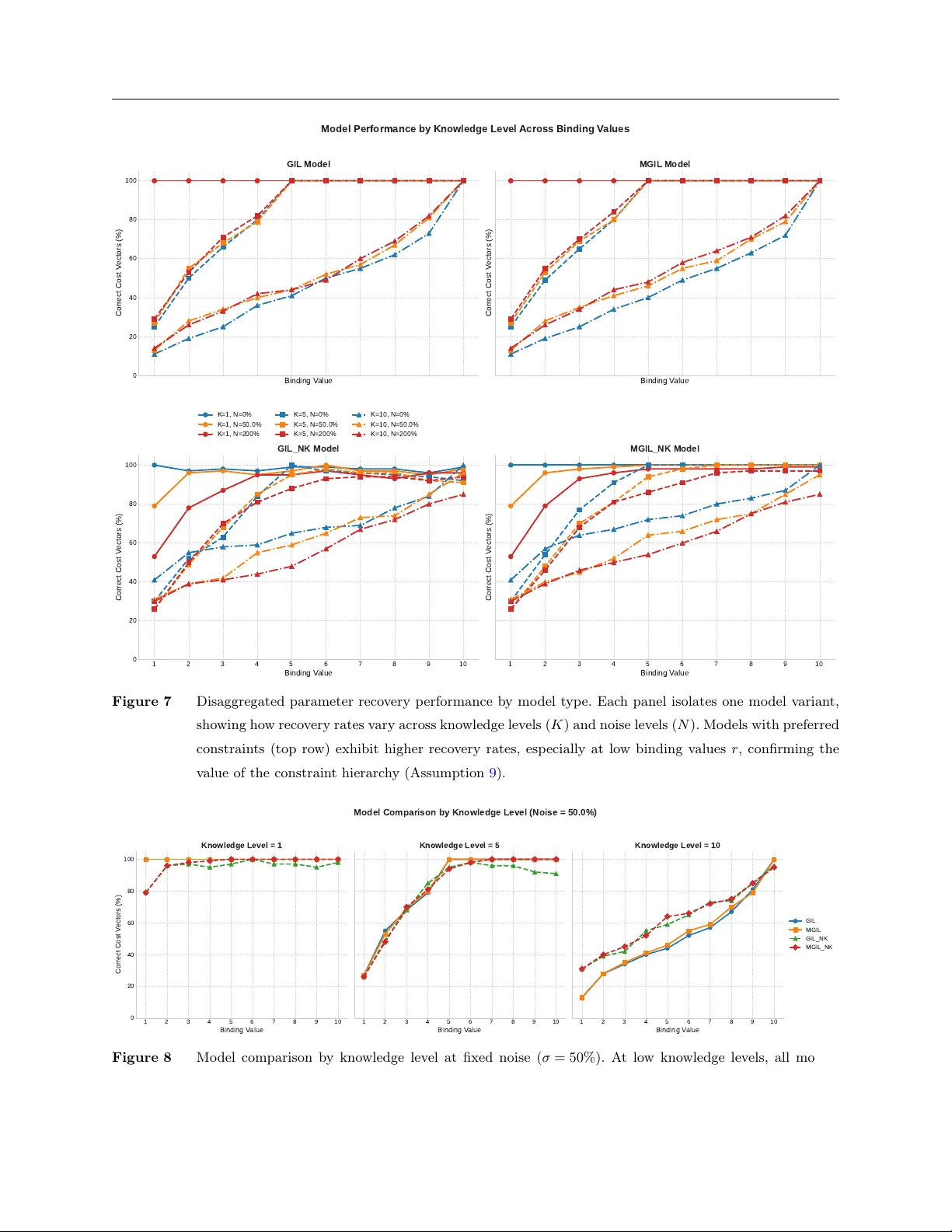
F rom Non-Iden tiﬁabilit y to Goal-In tegrated Decision-Making in P arametric In v erse Optimization F arzin Ahmadi, F ardin Ganjkhanlo o, Kimia Ghobadi Department of Civil and Systems Engineering, The Center for Systems Science and Engineering, The Malone Center for Engineering in Healthcare, Johns Hopkins University , Baltimore, MD 21218, fahmadi1@jh u.edu, fganjkh1@jhu.edu, kimia@jhu.edu In verse optimization seeks to recov er unknown ob jectiv e parameters from observ ed decisions, yet fundamen tal questions about when reco very is p ossible ha ve receiv ed limited formal treatment. This pap er dev elops a comprehensive theoretical framework for inv erse optimization in parametric conv ex mo dels. W e ﬁrst establish that non-identiﬁabilit y is the generic case: ev en with normalization and m ultiple observ ations, the parameter set compatible with data is generically multi-dimensional, and regularization do es not resolv e this. W e derive necessary and suﬃcient conditions for iden tiﬁabilit y . Motiv ated by these negative results, w e introduce the Inv erse Learning (IL) framework, which shifts the inferential target from the unknown parameter to the latent optimal solution, achieving a complexit y reduction that is indep endent of the num b er of observ ations. I L explicitly c haracterizes the full set of compatible parameters rather than returning an arbitrary elemen t. T o address the tension b etw een observ ational ﬁdelity and constrain t adherence, w e formalize the Observ ation-Constrain t T radeoﬀ and dev elop Goal-In tegrated In verse Learning mo dels that enable structured navigation of this sp ectrum with guaranteed monotonicity . Numerical exp eriments demonstrate sup erior solution accuracy , higher parameter recov ery rates, and signiﬁcant computational sp eedups. W e apply the framework to p ersonalized dietary recommendations using NHANES data, pro of- of-concept demonstrating improv ed glycemic control in a prospective feasibilit y study . Key words : in verse optimization, parametric con vex optimization, data-driven decision-making 1 F. Ahmadi is currently at the Deaprtmen t of Health Sciences, T o wson Universit y , T o wson, MD 21252. 1 F. Ganjkhanlo o is currently at the Cen ter for Health Systems and Policy Mo deling, Johns Hopkins Univ ersity , W ashington DC 20001. 1 Authors’ Names Blinded: Inverse L e arning 2 1. Intro duction A fundamen tal question in op erations research is ho w to infer the ob jectiv es driving observed decisions. When a decision-mak er rep eatedly solves an optimization problem whose constraints are kno wn but whose ob jectiv e function is not, the inverse optimization problem seeks to recov er the unkno wn parameters from observed solutions. Since the seminal form ulation b y Ahuja and Orlin ( 2001 ), in verse optimization has gro wn in to a mature metho dological area with applications spanning healthcare ( Chan et al. 2014 , Ajayi et al. 2022 ), transp ortation ( Cho w and Rec ker 2012 ), energy systems ( Saez-Gallego et al. 2017 , Ratliﬀ et al. 2014 ), and ﬁnance ( Bertsimas et al. 2012 , Utz et al. 2014 ). Recent surveys ( Chan et al. 2024 , Heub erger 2004 ) and methodological adv ances in statistical consistency ( Asw ani et al. 2018 ), online learning ( Dong et al. 2018 , Besb es et al. 2023 ), loss function design, and uncertaint y quan tiﬁcation ( Lin and Others 2024 ) hav e substan tially expanded the ﬁeld’s scop e and rigor. Despite this progress, t wo c hallenges hav e imp eded the practical deploymen t of in v erse optimization in data-rich settings. The ﬁrst is non-identiﬁability : when can the unkno wn ob jective parameters b e uniquely recov ered from observed decisions, and what happ ens when they cannot? The issue has b een ac knowledged in speciﬁc con texts, for instance, Asw ani et al. ( 2018 ) noted that constraints can render parameters unidentiﬁable, and Chan et al. ( 2019 ) dev elop ed closed- form solutions under sp ecial structures. How ever, a systematic characterization of when and why iden tiﬁability fails in general con vex mo dels has been lac king. The second c hallenge is c omputational sc alability : classical KKT-based inv erse formulations ha v e v ariables and constraints scaling linearly with the n um b er of observ ations. F or mo dern applications with thousands of observ ations, this scaling renders standard formulations impractical. This pap er addresses b oth c hallenges within a uniﬁed framew ork for parametric conv ex optimization. W e adopt a structured ob jectiv e with known conv ex basis functions and an unknown parameter v ector, encompassing linear programs, conv ex quadratic programs, and broader con vex mo dels as sp ecial cases. Our con tributions are organized around three interconnected themes. 1.1. Contributions 1. Non-iden tiﬁability is the generic case. W e provide, to our kno wledge, the ﬁrst comprehensive non-iden tiﬁability analysis for inv erse optimization in parametric con vex models. F or linear programs, w e c haracterize iden tiﬁabilit y through the geometry of normal cone intersections: parameter uniqueness requires the common normal cone to collapse to a single ray (Theorem 1 ), a condition that is generically violated whenever observ ations share tw o or more non-collinear activ e constrain t normals (Prop osition 2 ). F or general conv ex mo dels, w e identify tw o distinct sources of Authors’ Names Blinded: Inverse L e arning 3 am biguity , namely , normal cone dimensionality and basis function degeneracy , and sho w that the parameter feasibility set S is a polyhedral cone whose dimension depends on both the gradien t structure and the constraint geometry (Theorem 2 ). Critically , regularization do es not resolve non- iden tiﬁability; it can only enlarge the feasible parameter set (Corollary 1 ). W e then establish sharp suﬃcien t conditions for identiﬁabilit y based on a nov el ortho gonal p ersistent excitation condition: the excitation matrix must b e positive deﬁnite (Theorem 3 ). This condition is b oth necessary and suﬃcien t (Prop osition 5 ), precisely separating the iden tiﬁable and non-identiﬁable comp onents of the data’s information conten t. 2. Inv erse Learning: scalability and solution iden tiﬁability . Motiv ated b y the prev alence of non-identiﬁabilit y and the computational burden of classical form ulations, w e in tro duce Inverse L e arning (IL). Rather than imputing separate optimal solutions for eac h observ ation (as in classical in verse optimization), I L learns a single r epr esentative optimal solution that minimizes aggregate distance to observ ations while satisfying the KKT conditions for some parameter. This reform ulation ac hieves tw o k ey properties. First, problem complexit y drops to linear order of v ariables and constrain ts of the forward problem, indep endent of the numb er of observations K (Theorem 4 ). F or squared Euclidean loss, the data enter only through the sample centroid (Prop osition 6 ), enabling streaming up dates, parallelization, and memory-eﬃcient implemen tations. Second, I L ac hieves solution identiﬁability (uniqueness of the recov ered optimal solution) -under conditions that are strictly diﬀerent from, and in many practical settings less restrictive than, those required for parameter identiﬁabilit y (Theorem 7 ). I L do es not require one-dimensional normal cones or excitation conditions; it requires only lo cal conv exit y of the optimality set near the true solution. Rather than returning an arbitrary feasible parameter, I L explicitly characterizes the full set of compatible parameters (Theorem 5 ), making non-uniqueness transparent. 3. The Observ ation-Constraint T radeoﬀ and Goal-Integrated mo dels. W e formalize the tension b etw een ﬁtting observed behavior and enforcing domain constraints as the Observation- Constr aint T r ade oﬀ (Deﬁnition 2 ) and dev elop Go al-Inte gr ate d Inverse L e arning mo dels to navigate it. G I L controls the num b er r of binding relev an t constraints via a cardinality parameter, enabling systematic exploration of the tradeoﬀ sp ectrum. MG I L pro vides structured sequen tial na vigation b y iteratively adding constraints while inheriting previously active ones, yielding monotone distance sequences (Theorem 10 ) o v er nested faces (Theorem 11 ). Both mo dels preserv e the K -independence of I L , enforce complete KKT conditions guaran teeing forward optimalit y , and characterize the compatible parameter set at each solution. A constrain t hierarch y—relev an t (exp ert knowledge), preferred (priorit y subset), and trivial (structural feasibility)—supports data-driven constrain t selection while maintaining mathematical v alidity . Authors’ Names Blinded: Inverse L e arning 4 1.2. Relevant Literature The inv erse optimization literature has ev olved along sev eral in terrelated threads. The classical strand, initiated by Ah uja and Orlin ( 2001 ) and developed by Heub erger ( 2004 ), Iyengar and Kang ( 2005 ), Chan et al. ( 2014 ), fo cuses on reco vering parameters under the assumption that observ ations are exactly optimal. The data-driven strand relaxes this assumption, accommo dating noisy or sub optimal observ ations through loss-function-based formulations ( Keshav arz et al. 2011 , Bertsimas et al. 2015 , Asw ani et al. 2018 , Esfahani et al. 2018 ). Recent work has further extended these foundations: Besb es et al. ( 2023 ) develop oﬄine and online contextual inv erse optimization with logarithmic regret b ounds, introducing the circumcen ter p olicy and ellipsoidal cone machinery for minimax regret; Zattoni Scro ccaro et al. ( 2025 ) prop ose the complementary incenter cost vector with tractable con v ex reformulations, introduce the augmented sub optimality loss (ASL) as a relaxation for inconsistent data, and develop a stochastic appro ximate mirror descen t algorithm with pro v able conv ergence rates; Lin and Others ( 2024 ) prop ose conformal in verse optimization, learning uncertain ty sets rather than point estimates; and Shahmoradi and Lee ( 2022 ) dev elop quan tile-based approac hes to improv e stability . Our work intersects with but is distinct from these con tributions in sev eral resp ects. First, while identiﬁabilit y has b een discussed as a technical assumption supp orting consistency results ( Asw ani et al. 2018 ) or as a geometric property of sp eciﬁc mo dels ( Chan et al. 2019 ), w e pro vide a systematic analysis establishing that non-identiﬁabilit y is structurally inherent in inv erse con vex optimization. Our orthogonal excitation condition oﬀers a precise geometric characterization that uniﬁes and extends scattered conditions in the literature. Second, whereas classical and data-driv en approac hes b oth scale linearly in K , our I L framework eliminates this dep endence en tirely through a reform ulation that targets the laten t solution rather than the parameter—a fundamen tally diﬀerent inferen tial ob jectiv e. Third, the Goal-Integrated framew ork addresses a gap largely unaddressed in the in verse optimization literature: the in tegration of domain exp ertise through constraint hierarc hies and con trolled constraint activ ation, pro viding practitioners with in terpretable mechanisms to balance data ﬁdelity against normative goals. The observ ation-constraint tradeoﬀ that w e formalize also connects to the broader literature on decision-a ware learning ( Elmach toub and Grigas 2022 ) and prescriptive analytics, where the goal is not merely to estimate parameters but to generate actionable decisions. Our framework provides a structured path from descriptiv e (what do people do?) through normativ e (what should they do?) to prescriptiv e (what achiev able c hanges would improv e outcomes?), a progression of particular v alue in b eha vioral applications. F rom an application p erspective, p ersonalized health in terv en tions and dietary recommendations in particular represent a natural domain for in verse optimization. Observ ed dietary b eha viors reﬂect Authors’ Names Blinded: Inverse L e arning 5 laten t preferences that may conﬂict with clinical guidelines, and the gap b etw een p opulation-level recommendations and individual adherence remains a signiﬁcant challenge ( Sac ks et al. 2001 , Liese et al. 2009 ). Our framework addresses this gap b y generating recommendations that resp ect habitual patterns while progressiv ely incorporating n utritional constrain ts, with eac h step quantifying the marginal b eha vioral cost of additional guideline adherence. The remainder of this pap er is organized as follows. Section 2 formalizes the in verse optimization problem for parametric conv ex mo dels, establishes the non-identiﬁabilit y results, and derives iden tiﬁability conditions. Section 3 dev elops the Inv erse Learning framework, including complexity reduction, statistical guarantees, and solution iden tiﬁability . Section 4 in tro duces the Goal- In tegrated mo dels (GIL and MG I L ) and the Observ ation-Constraint T radeoﬀ. Section 5 presen ts n umerical experiments comparing the I L framew ork against classical inv erse optimization. Section 6 applies the metho dology to p ersonalized dietary recommendations using NHANES data and a prosp ectiv e feasibilit y study . Section EC.2 in the electronic companion describes the interactiv e decision-supp ort to ols dev elop ed to op erationalize the framew ork. 2. Inverse Optimization fo r P arametric Convex Models 2.1. Prelimina ries W e adopt a structured parametric ob jective of the form f ( x, θ ) = p X j =1 θ j ϕ j ( x ) , (1) where θ = ( θ 1 , . . . , θ p ) ⊤ ∈ R p are unknown parameters and ϕ j : R n → R are known, contin uously diﬀeren tiable conv ex basis functions. T o ensure that F O ( θ , Ω) is a con v ex optimization problem for every admissible parameter vector, we restrict attention to nonnegative combinations of conv ex basis functions, i.e., θ ∈ R p + (see Assumption 3 ). Under this restriction, f ( · , θ ) is conv ex on Ω . This parametric form cov ers several standard mo dels: (i) for linear programs, ϕ j ( x ) = x j yields f ( x, θ ) = θ ⊤ x ; and (ii) for conv ex quadratic programs, ϕ j ( x ) = x ⊤ Q j x with Q j ⪰ 0 (and optionally aﬃne terms ϕ j ( x ) = x i ) yields f ( x, θ ) = x ⊤ ( P j θ j Q j ) x + c ( θ ) ⊤ x with a p ositive semideﬁnite quadratic term. W e base our metho dology on the following assumptions. Assumption 1 (Basis F unction Prop erties) . W e assume: (i) { ϕ j } p j =1 ar e line arly indep endent on Ω ; (ii) some ϕ j 0 is non-c onstant on Ω ; (iii) e ach ϕ j is c onvex and c ontinuously diﬀer entiable on Ω ; and (iv) the gr adient matrix [ ∇ ϕ 1 ( x ) · · · ∇ ϕ p ( x )] has r ank at le ast min( p, n ) for generic x ∈ Ω . Assumption 2 (Constraint Qualiﬁcation and Smo othness) . The c onstr aint functions g i : R n → R ar e c onvex and c ontinuously diﬀer entiable. The fe asible set Ω = { x ∈ R n : g i ( x ) ≤ 0 , i = 1 , . . . , m } satisﬁes Slater’s c ondition: ther e exists ˆ x ∈ R n such that g i ( ˆ x ) < 0 for al l i . Authors’ Names Blinded: Inverse L e arning 6 Assumption 3 (Parameter Normalization) . T o avoid sc ale invarianc e and pr eserve c onvexity of f ( · , θ ) , we r estrict p ar ameters to Θ =  θ ∈ R p + : ∥ θ ∥ q = 1 , θ j 0 ≥ α > 0  , (2) wher e q ∈ [1 , ∞ ] and α > 0 ensur es the non-c onstant b asis function ϕ j 0 r e c eives nonzer o weight. Giv en noisy observ ations X = { x k : k = 1 , . . . , K } , the in verse conv ex optimization problem seeks parameters θ suc h that eac h observ ation is close to an optimal solution of F O ( θ , Ω) . Under Assumption 2 , the following KKT-based formulation enforces optimality: I C O ( X , Ω) : min θ, { λ k } , { z k } K X k =1 ∥ x k − z k ∥ 2 2 (3) s.t. z k ∈ Ω , ∀ k , p X j =1 θ j ∇ ϕ j ( z k ) + m X i =1 λ k i ∇ g i ( z k ) = 0 , ∀ k , λ k i g i ( z k ) = 0 , ∀ i, k , λ k ∈ R m + , ∀ k , θ ∈ Θ . This enforces the Karush–Kuhn–T uck er (KKT) conditions of the forward problem. As is w ell known from the literature on in verse linear and con v ex optimization (see, e.g., Ah uja and Orlin 2001 , Chan et al. 2014 , Aswani et al. 2018 ), this problem is generally noncon v ex and NP-hard due to complemen tarity constrain ts. Under Slater’s condition (Assumption 2 ), the KKT conditions are b oth necessary and suﬃcien t for optimality of z k in the forw ard problem, and strong dualit y holds. When ϕ j ( x ) = x j and g i ( x ) = b i − a ⊤ i x , the problem reduces to the classical in verse linear optimization mo del: I LO ( X , Ω) : min θ, { λ k } , { z k } K X k =1 ∥ x k − z k ∥ 2 2 (4) s.t. Az k ≥ b, ∀ k , θ = A ⊤ λ k , ∀ k , θ ⊤ z k = b ⊤ λ k , ∀ k , λ k ∈ R m + , ∀ k , ∥ θ ∥ q = 1 . Note that in the linear case, the stationarity condition θ = A ⊤ λ k com bined with primal feasibility Az k ≥ b , dual feasibilit y λ k ≥ 0 , and the strong dualit y equalit y θ ⊤ z k = b ⊤ λ k together imply complemen tary slackness: λ k i ( a ⊤ i z k − b i ) = 0 for all i, k . This form ulation has b een studied extensiv ely (e.g., Chan et al. 2014 , Bertsimas et al. 2015 ) and admits tractable con vex reform ulations under certain norms and error measures. Ho wev er, Authors’ Names Blinded: Inverse L e arning 7 computational scaling issues persist with large datasets. F ollowing Keshav arz et al. ( 2011 ) and Asw ani et al. ( 2018 ), a regularized version relaxes the KKT conditions by a tolerance ϵ > 0 : R - I C O ( X , Ω , ϵ ) : min θ, { λ k } , { z k } K X k =1 ∥ x k − z k ∥ 2 2 (5) s.t. g i ( z k ) ≤ ϵ, ∀ i, k , λ k ∈ R m + , ∀ k ,    p X j =1 θ j ∇ ϕ j ( z k ) + m X i =1 λ k i ∇ g i ( z k )    2 ≤ ϵ, ∀ k , θ ∈ Θ . This relaxation impro ves robustness to noise and av oids exact complementarit y constraints. Under Assumptions 1 – 3 , iden tiﬁabilit y of θ requires suﬃcien tly ric h observ ations. If the basis ev aluations { ϕ j ( x k ) } are linearly indep enden t across k , then distinct parameters yield distinct ob jective functions, ensuring uniqueness up to normalization. Similar rank conditions app ear in Bertsimas et al. ( 2015 ) and Aswani et al. ( 2018 ). Remark 1 (St a tistical Consistency). When observ ations are generated as x k = x ∗ ( θ 0 ) + ξ k with zero-mean noise, estimators based on R - I C O are statistically consistent under regularity conditions ( Aswani et al. 2018 ). The con vergence rate dep ends on the noise v ariance, the num b er of samples K , and the geometry of the basis functions. Consistency of the p ar ameter estimator strictly requires the mo del to b e iden tiﬁable. As we establish in Section 2.2 , these identiﬁabilit y conditions are generically violated in practice. Remark 2 (Comput a tional Complexity). F or general con vex basis functions, b oth I C O and R - I C O are nonconv ex due to bilinearities in ( 3 ) and complementarit y constraints; only local or heuristic methods are tractable in general. F or the linear case with aﬃne ϕ j and g i , the relaxed form ulation R - I C O reduces to a conv ex quadratic or second-order cone program, hence polynomial- time solv able via interior-point metho ds. The exact formulation I C O remains NP-hard even in the linear case due to complemen tarity constraints. F or quadratic or nonlinear forward mo dels, R - I C O remains biconv ex, and global tractabilit y is not guaran teed; in practice, alternating optimization and conv ex relaxations are used ( Aswani et al. 2018 ). When F O ( θ , Ω) admits m ultiple optimal solutions, the inv erse form ulation imputes v ariables z k that pro ject each observ ation x k on to the corresp onding optimal set, thereby resolving non uniqueness of solutions for a ﬁxed θ . How ev er, ev en with multiple (p ossibly noisy) observ ations, more than one parameter vector θ often rationalizes the data equally w ell. In linear mo dels, an y ob jectiv e v ector within the cone spanned b y active constraint normals yields the same optimal face. The in verse optimization framew ork mitigates this am biguity b y enforcing join t consistency Authors’ Names Blinded: Inverse L e arning 8 across all samples and b y imp osing normalization, but uniqueness of θ is rarely guaranteed. As suc h, the feasible set of parameters may remain large, and the solution to I C O or R - I C O should b e in terpreted as one element of a p otentially non-unique set. 2.2. Non-Identiﬁabilit y of I C O and R - I C O In general, the in v erse problems I C O and R - I C O are set-value d , i.e., even with normalization, the parameter θ ∈ Θ compatible with a dataset need not b e unique. W e establish this for the inv erse linear case and then extend the analysis to general conv ex mo dels. Let Ω = { x ∈ R n : Ax ≥ b } with ro ws a ⊤ i of A ∈ R m × n , and let f ( x, θ ) = θ ⊤ x (i.e., ϕ j ( x ) = x j ). F or z ∈ Ω , let I ( z ) := { i : a ⊤ i z = b i } denote the active set, and let N Ω ( z ) = cone { a i : i ∈ I ( z ) } be the normal cone at z . The forw ard KKT conditions imply that any optimal z m ust satisfy θ ∈ N Ω ( z ) , up to scaling. Pr oposition 1 (Normal Cone Intersection Structure) . L et { z k } K k =1 ⊆ Ω b e impute d optima. Deﬁne the c ommon normal c one interse ction C := K \ k =1 N Ω ( z k ) . Then C is a p olyhe dr al c one. Mor e over, let I ∩ := T K k =1 I ( z k ) denote the c ommon active set. Then: (i) cone { a i : i ∈ I ∩ } ⊆ C . (ii) If I ∩  = ∅ , then C is nonempty. (iii) C r e duc es to a single r ay if and only if dim( C ) = 1 . The following prop osition establishes explicit conditions under which C contains multiple rays, whic h is the key requirement for non-identiﬁabilit y . Pr oposition 2 (Conditions for Multiple Rays in C ) . L et C = T K k =1 N Ω ( z k ) and let I ∩ = T K k =1 I ( z k ) . The c one C c ontains at le ast two distinct r ays under any of the fol lowing c onditions: (i) (R ich c ommon active set) | I ∩ | ≥ 2 and the ve ctors { a i : i ∈ I ∩ } ar e not al l c ol line ar, i.e., dim(span { a i : i ∈ I ∩ } ) ≥ 2 . (ii) (Single observation at non-simple vertex) K = 1 and | I ( z 1 ) | ≥ 2 with { a i : i ∈ I ( z 1 ) } not al l c ol line ar. (iii) (A ligne d active sets) F or al l k , the active sets satisfy I ( z 1 ) ⊆ I ( z k ) , and c ondition (ii) holds for z 1 . Conversely, C is a single r ay if and only if dim( C ) = 1 , which r e quir es the observations to c ol le ctively imp ose suﬃcient line arly indep endent r estrictions on fe asible obje ctive dir e ctions to le ave exactly one de gr e e of fr e e dom. Authors’ Names Blinded: Inverse L e arning 9 Condition (ii) of Prop osition 2 is satisﬁed at any vertex of a p olyhedron in R n where at least n constraints are active with linearly indep endent normals (the generic case). Ev en with multiple observ ations, condition (i) holds whenever all observ ations share at least tw o non-collinear active constrain t normals—a common occurrence when observ ations cluster near a particular face or vertex. The single-ra y case dim( C ) = 1 is thus non-generic and requires precise geometric alignmen t across observ ations. W e now state the main non-identiﬁabilit y theorem for in verse linear programming. Theorem 1 (Non-Identiﬁabilit y of I C O in Linear Programs) . L et { z k } K k =1 ⊆ Ω b e impute d optima and let C = T K k =1 N Ω ( z k ) . If any of the c onditions in Pr op osition 2 hold, then the fe asible set C ∩ Θ c ontains at le ast two distinct p oints for any normalization set Θ of the form Θ = { θ : ∥ θ ∥ 2 = 1 } or Θ = { θ : 1 ⊤ θ = 1 , θ ≥ 0 } . Conse quently, I C O admits multiple fe asible p ar ameters for the same dataset, and the inverse pr oblem is non-identiﬁable. Cor ollar y 1 (P ersistence of Non-Iden tiﬁabilit y Under Regularization) . Under the c onditions of The or em 1 , the fe asible set of R - I C O ( X , Ω , ϵ ) also c ontains multiple fe asible θ for al l ϵ ≥ 0 . That is, r e gularization do es not r esolve the non-identiﬁability pr esent in I C O . W e now extend the non-identiﬁabilit y analysis to parametric conv ex ob jectives of the form f ( x, θ ) = P p j =1 θ j ϕ j ( x ) . Let A ( z ) := [ ∇ ϕ 1 ( z ) · · · ∇ ϕ p ( z )] ∈ R n × p denote the matrix of basis function gradien ts ev aluated at z . The KKT stationarity condition for z to b e optimal can b e written as A ( z ) θ ∈ − N Ω ( z ) . (6) F or a collection of imputed optima { z k } K k =1 , deﬁne the parameter feasibility set S := K \ k =1  θ ∈ R p : A ( z k ) θ ∈ − N Ω ( z k )  . (7) Pr oposition 3 (F easibilit y Set Structure for Con v ex Mo dels) . The set S is a (p ossibly empty) p olyhe dr al c one in R p . Its dimension dep ends on b oth the r ank structur e of the gr adient matric es { A ( z k ) } K k =1 and the dimensions of the normal c ones { N Ω ( z k ) } K k =1 . Pr oposition 4 (Conditions for Non-Identiﬁabilit y in Conv ex Mo dels) . The set S c ontains at le ast two non-c ol line ar r ays (henc e S ∩ Θ c ontains multiple p oints for standar d normalizations) under any of the fol lowing c onditions: (i) T K k =1 k er( A ( z k ))  = { 0 } , i.e., ther e exists θ 0  = 0 with A ( z k ) θ 0 = 0 for al l k , and S c ontains at le ast one element ¯ θ not p ar al lel to θ 0 . (ii) F or some k 0 , dim( N Ω ( z k 0 )) ≥ 2 , A ( z k 0 ) has ful l c olumn r ank p , and dim  range( A ( z k 0 )) ∩ N Ω ( z k 0 )  ≥ 2 Authors’ Names Blinded: Inverse L e arning 10 (a) Single observ ation at v ertex g 1 g 2 g 3 g 5 Ω z 1 a 2 a 3 θ (1) θ (2) N Ω ( z 1 ) | I ( z 1 ) | = 2 with non-collinear a 2 , a 3 ⇒ dim( N Ω ( z 1 )) = 2 ⇒ Multiple θ feasible (Prop. 2 (ii)) (b) Intersection C = T k N Ω ( z k ) Ω z 1 N Ω ( z 1 ) z 2 N Ω ( z 2 ) C shared If dim( C ) = 1 : unique θ (up to scale) If dim( C ) ≥ 2 : non-identiﬁable (Thm. 1 ) Generic case: dim( C ) ≥ 2 Figure 1 Geometric Illustration of non-identiﬁabilit y in inv erse linear optimization. (a) At a vertex z 1 where tw o non-collinear constraints are active, the normal cone N Ω ( z 1 ) is tw o-dimensional, admitting multiple feasible parameters θ (1) , θ (2) ∈ N Ω ( z 1 ) ∩ Θ (Prop osition 2 (ii)). (b) With tw o observ ations z 1 , z 2 , the feasible parameter set is the intersection C = N Ω ( z 1 ) ∩ N Ω ( z 2 ) . Non-identiﬁabilit y p ersists unless observ ations reduce C to a single ray (Theorem 1 ). (iii) The excitation matrix S = P K k =1 A ( z k ) ⊤ P k A ( z k ) is singular, S is non-empty, and ther e exists ¯ θ ∈ S not p ar al lel to any ∆ θ ∈ ker( S ) \ { 0 } . The rank of the excitation matrix satisﬁes rank( S ) ≤ P K k =1 rank( P k A ( z k )) ≤ K ( p − 1) (eac h summand has rank at most min( n − 1 , p ) ≤ p − 1 under Assumption 5 ). Hence S is necessarily singular when K ( p − 1) < p , i.e., K < p/ ( p − 1) . F or p ≥ 2 this gives K < 2 , conﬁrming the intuition that a single observ ation is generically insuﬃcient for iden tiﬁability in m ulti-parameter mo dels. More generally , for S ≻ 0 one typically needs K ≥ p observ ations with suﬃcient geometric diversit y (Corollary 2 ). The condition dim(range( A ( z k 0 )) ∩ N Ω ( z k 0 )) ≥ 2 is automatically satisﬁed in the follo wing cases: (a) Linear programs: A ( z ) = I n for all z , so range( A ) = R n and the condition reduces to dim( N Ω ( z k 0 )) ≥ 2 . (b) Ov erparameterized mo dels ( p ≥ n ): A ( z k 0 ) maps R p on to R n , so again range( A ) = R n . (c) Generic p osition with p + dim( N Ω ( z k 0 )) > n + 1 : a p -dimensional subspace generically in tersects a d -dimensional cone in dimension max( p + d − n, 0) , which is ≥ 2 when p + d ≥ n + 2 . Theorem 2 (Global Non-Iden tiﬁabilit y in Con vex In verse Optimization) . If any of the c onditions in Pr op osition 4 hold, then b oth I C O and R - I C O admit multiple fe asible p ar ameters θ , and the inverse pr oblem is glob al ly non-identiﬁable. Authors’ Names Blinded: Inverse L e arning 11 Remark 3 (Sources of Ambiguity in Convex Models). Equation ( 6 ) reveals tw o distinct sources of parameter ambiguit y: (i) Normal cone dimensionalit y: If N Ω ( z k ) is high-dimensional (e.g., when z k lies at a vertex with man y active constraints), m ultiple ob jective gradien t directions − A ( z k ) θ can supp ort the same optimum. (ii) Basis function degeneracy: If A ( z k ) is rank-deﬁcient, then distinct parameter vectors θ can map to the same gradient ∇ x f ( z k , θ ) . Uniqueness of θ requires b oth that the data suﬃcien tly excite the basis directions (making the stack ed matrix [ A ( z 1 ) ⊤ · · · A ( z K ) ⊤ ] ⊤ ha ve full column rank) and that the intersection of normal cones collapse to a single ray . Absent these strong conditions—which are generically violated—the inv erse problem remains set-v alued. In R - I C O , the exact stationarit y condition ( 6 ) is relaxed to dist( A ( z k ) θ , − N Ω ( z k )) ≤ ϵ , whic h only enlarges the feasible set. An y non-uniqueness present in I C O p ersists under regularization, and additional am biguit y ma y b e in tro duced unless further structure, suc h as strong con v exity , full-rank conditions, or explicit priors, is imposed. This motiv ates the alternative approaches developed in subsequen t sections. 2.3. Suﬃcient Conditions fo r P arameter Identiﬁabilit y The non-iden tiﬁability results of Theorems 1 – 2 establish that parameter recov ery is generically set- v alued. W e no w pro vide suﬃcien t conditions under whic h the inv erse parameter b ecomes unique (up to normalization). These conditions directly address the tw o sources of am biguit y iden tiﬁed in Remark 3 . Assumption 4 (Strong Con v exity in Decision V ariable) . F or every θ ∈ Θ , the function x 7→ f ( x, θ ) = P p j =1 θ j ϕ j ( x ) is µ -str ongly c onvex on Ω for some µ > 0 indep endent of θ . Strong conv exity ensures that the forward problem F O ( θ , Ω) admits a unique optimal solution x ∗ ( θ ) for eac h θ . This eliminates ambiguit y in the forw ard direction but do es not, b y itself, guaran tee iden tiﬁability of the inv erse problem. Assumption 5 (One-Dimensional Normal Cones) . F or e ach impute d optimum z k , the normal c one is one-dimensional: N Ω ( z k ) = cone { n k } , with ∥ n k ∥ 2 = 1 . Assumption 5 directly addresses the ﬁrst source of non-identiﬁabilit y from Proposition 2 (ii): it rules out high-dimensional normal cones by requiring eac h z k to lie on a smo oth p ortion of the b oundary ∂ Ω where exactly one constrain t is active, or more generally , where the active constrain t normals are collinear. Authors’ Names Blinded: Inverse L e arning 12 Assumption 6 (Orthogonal P ersisten t Excitation) . L et A ( z ) := [ ∇ ϕ 1 ( z ) · · · ∇ ϕ p ( z )] ∈ R n × p denote the gr adient matrix and P k := I n − n k ( n k ) ⊤ the ortho gonal pr oje ction onto the hyp erplane p erp endicular to n k . The fol lowing excitation matrix is p ositive deﬁnite, S ≻ 0 : S := K X k =1 A ( z k ) ⊤ P k A ( z k ) ∈ R p × p . Assumption 6 addresses the second source of non-identiﬁabilit y from Prop osition 4 (i): it ensures that no nonzero parameter p erturbation ∆ θ can pro duce gradient chan ges lying en tirely along the normal directions { n k } . The pro jection P k extracts the comp onen t of A ( z k )∆ θ orthogonal to n k , and p ositiv e deﬁniteness of S ensures this orthogonal comp onen t is nonzero for any ∆ θ  = 0 . Remark 4. The matrix S measures how well the observ ations { z k } excite the parameter space in directions distinguishable from rescaling the dual m ultipliers. Consider the KKT condition A ( z k ) θ = − α k n k for some α k ≥ 0 . A p erturbation θ → θ + ∆ θ can b e absorb ed b y adjusting α k → α k + ∆ α k if and only if A ( z k )∆ θ is parallel to n k . The condition S ≻ 0 ensures that across all observ ations, no suc h hidden p erturbation direction exists. Theorem 3 (Parameter Iden tiﬁability Under Orthogonal Excitation) . Under Assumptions 4 – 6 , and a normalization c onvention θ ∈ Θ (e.g., ∥ θ ∥ 2 = 1 with a sign c onvention, or 1 ⊤ θ = 1 with θ ≥ 0 ), the p ar ameter θ solving I C O is unique. Pr oposition 5 (Necessity of Orthogonal Excitation for Identiﬁabilit y) . Under Assumptions 4 – 5 , if S = P K k =1 A ( z k ) ⊤ P k A ( z k ) is singular, then ther e exist distinct p ar ameters θ , θ ′ ∈ R p (prior to normalization) that b oth satisfy the KKT c onditions at al l impute d optima { z k } K k =1 . Conse quently, I C O admits multiple solutions, and identiﬁability fails. The n ull space of S characterizes the unidentiﬁable directions in parameter space: p erturbations ∆ θ ∈ k er( S ) pro duce gradien t changes A ( z k )∆ θ that are entirely absorb ed by adjusting the dual m ultipliers α k . These directions are in visible to the in v erse problem and represen t fundamental limitations of the av ailable data. An alternativ e identiﬁabilit y approach requires the stac ked gradient matrix ¯ A := [ A ( z 1 ) ⊤ · · · A ( z K ) ⊤ ] ⊤ ∈ R K n × p to ha ve full column rank. This condition is neither necessary nor suﬃcien t for identiﬁabilit y: (i) Not ne c essary: Ev en if ¯ A is rank-deﬁcient, S may still be p ositive deﬁnite if the rank deﬁciency o ccurs along normal dire ctions that are pro jected aw ay . (ii) Not suﬃcient: Ev en if ¯ A has full rank, parameter p erturbations along normal directions can remain uniden tiﬁable if dim( N Ω ( z k )) > 1 , violating Assumption 5 . The orthogonal excitation condition precisely captures the identiﬁable information conten t of the data. Authors’ Names Blinded: Inverse L e arning 13 Remark 5. The matrix M := P K k =1 A ( z k ) ⊤ n k ( n k ) ⊤ A ( z k ) captures alignment of gradien t directions along the normals n k . Note the decomp osition S + M = P k A ( z k ) ⊤ A ( z k ) , the standard Gramian. While M measures how w ell the data determine the dual multipliers α k , it is S that go verns parameter iden tiﬁabilit y: M ≻ 0 alone do es not imply identiﬁabilit y; S ≻ 0 is both necessary and suﬃcien t (under Assumptions 4 – 5 ); and the decomp osition separates the Gramian in to identiﬁable ( S ) and non-identiﬁable ( M ) comp onents. The positive deﬁniteness of S may b e diﬃcult to v erify a priori since it depends on the (unkno wn) imputed optima { z k } . W e provide simpler suﬃcient conditions. Cor ollar y 2 (Suﬃcien t Conditions for P ositive Deﬁnite S ) . Assumption 6 ( S ≻ 0 ) is satisﬁe d if either of the fol lowing holds: (i) The normal dir e ctions { n k } K k =1 sp an R n , and for e ach k , A ( z k ) has ful l c olumn r ank p . (ii) A t le ast one observation z k 0 lies in the interior of Ω (so N Ω ( z k 0 ) = { 0 } and P k 0 = I ), and A ( z k 0 ) has ful l c olumn r ank. Corollary 2 (ii) indicates that iden tiﬁability is easiest to ac hieve when some observ ations corresp ond to interior optima. In constrained settings, condition (i) requires geometric diversit y in the activ e constraints across observ ations, which is a form of exp erimental design for in v erse optimization. When these conditions fail, the practitioner should exp ect set-v alued parameter reco very and may employ the characterization metho ds dev elop ed in subsequen t sections. 3. Inverse Learning: A Scalable Framew o rk fo r Data-Rich Inverse Optimization The classical form ulations I C O and R - I C O face tw o fundamen tal c hallenges in data-rich settings: (i) Computational in tractability: I C O requires O ( K n + K m ) v ariables and O ( K m ) constrain ts. F or mo dern applications with thousands of data p oin ts, this scaling renders classical form ulations impractical. (ii) Inheren t non-iden tiﬁabilit y: Theorems 1 – 2 establish that parameter reco very is generically set-v alued. Classical approac hes either ignore this m ultiplicit y (returning an arbitrary feasible θ ) or require stringen t conditions (Theorem 3 ) that are rarely satisﬁed in practice. W e prop ose Inverse L e arning ( I L ), whic h addresses b oth challenges through a fundamental reform ulation: rather than imputing K separate optimal solutions { z k } K k =1 , I L learns a single r epr esentative optimal solution z ∗ ∈ Ω that b est ﬁts the observed data. This approach targets settings where observ ations are noisy measuremen ts of a common laten t optimal decision—a natural assumption when a single decision-maker’s b ehavior is observed rep eatedly under noise. Authors’ Names Blinded: Inverse L e arning 14 3.1. The Inverse Lea rning F ormulation Giv en observ ations X = { x k } K k =1 and feasible set Ω , the In verse Learning problem seeks a single optimal solution z ∗ suc h that: (1) z ∗ minimizes the aggregate distance to observ ations; (2) z ∗ is optimal for F O ( θ , Ω) for some θ ∈ Θ ; and (3) the set of all compatible parameters Θ ∗ ( z ∗ ) is c haracterized. The I L mo del can b e written as follows: I L ( X , Ω) : min z ,θ,λ K X k =1 ∥ x k − z ∥ 2 2 (8a) s.t. g i ( z ) ≤ 0 , i = 1 , . . . , m, (8b) p X j =1 θ j ∇ ϕ j ( z ) + m X i =1 λ i ∇ g i ( z ) = 0 , (8c) λ i g i ( z ) = 0 , i = 1 , . . . , m, (8d) λ ≥ 0 , θ ∈ Θ . (8e) The ob jectiv e ( 8a ) minimizes aggregate squared error. Constraint ( 8b ) ensures primal feasibilit y . Constrain ts ( 8c )–( 8e ) enco de the KKT conditions, ensuring z is optimal for some forward problem with parameters ( θ , λ ) . Theorem 4 (Complexity Reduction) . The pr oblem I L ( X , Ω) has O ( n + p + m ) variables and O ( n + m ) c onstr aints, independent of the num b er of observ ations K . In c ontr ast, I C O ( X , Ω) has O ( K n + p + K m ) variables and O ( K n + K m ) c onstr aints. Theorem 4 establishes data sc alability : the problem size is indep endent of K (See T able 1 for summary comparison). How ever, I L remains nonconv ex due to bilinear terms in ( 8c ) and complemen tarity constrain ts ( 8d ). The computational adv antage lies in the ability to process arbitrarily large datasets through aggregated statistics (Prop osition 6 ) and problem size reduction indep enden t of K , not in polynomial-time solv abilit y . F or the linear case with polyhedral Ω , complemen tarity can b e handled via mixed-integer programming with O ( m ) binary v ariables, indep enden t of K . Pr oposition 6 (Data Aggregation Prop ert y) . The obje ctive function satisﬁes K X k =1 ∥ x k − z ∥ 2 2 = K ∥ z − ¯ x ∥ 2 2 + K X k =1 ∥ x k − ¯ x ∥ 2 2 , (9) wher e ¯ x = 1 K P K k =1 x k is the sample c entr oid. Conse quently, I L ( X , Ω) is e quivalent to min z ,θ,λ K ∥ z − ¯ x ∥ 2 2 s.t. ( 8b ) – ( 8e ) , (10) which dep ends on the data only thr ough the c entr oid ¯ x . Authors’ Names Blinded: Inverse L e arning 15 The reduction ( 9 ) is speciﬁc to squared Euclidean loss. F or ℓ 1 loss, the analogous aggregation uses the component wise median. F or general ℓ p losses with p  = 1 , 2 , no ﬁnite-dimensional aggregation exists, and the solv er must retain all K data p oints. The scalabilit y of I L via aggregation is thus loss-dep enden t, though the constraint-side complexity reduction (Theorem 4 ) holds univ ersally . The aggregation prop erty enables: (i) Streaming up dates: ¯ x K +1 = K K +1 ¯ x K + 1 K +1 x K +1 ; (ii) P arallelization: partial cen troids from data partitions can b e combined via weigh ted av eraging; and (iii) Memory eﬃciency: only ¯ x ∈ R n need b e stored, not the full dataset X ∈ R n × K . 3.2. Cha racterization of I L Prop erties Unlik e classical IO, which returns a single (often arbitrary) feasible parameter, I L explicitly c haracterizes all compatible parameters. Under Assumption 2 , the KKT conditions are necessary and suﬃcient for optimality , and the normal cone admits the representation N Ω ( z ) =    X i ∈ I ( z ) µ i ∇ g i ( z ) : µ i ≥ 0    = cone {∇ g i ( z ) : i ∈ I ( z ) } , (11) where I ( z ) = { i : g i ( z ) = 0 } is the active set. Theorem 5 (Parameter Set Characterization) . L et ( z ∗ , θ ∗ , λ ∗ ) solve I L ( X , Ω) . Deﬁne the active set I ( z ∗ ) = { i : g i ( z ∗ ) = 0 } . Under Assumption 2 , the set of al l p ar ameters for which z ∗ is optimal is Θ ∗ ( z ∗ ) = { θ ∈ Θ : A ( z ∗ ) θ ∈ − N Ω ( z ∗ ) } , (12) wher e A ( z ∗ ) = [ ∇ ϕ 1 ( z ∗ ) · · · ∇ ϕ p ( z ∗ )] and N Ω ( z ∗ ) is given by ( 11 ) . F or the linear case, I L admits a geometric characterization that clariﬁes its structure. Assumption 7 (Regularity for Consistency) . The fol lowing c onditions hold: (i) Θ is c omp act and the mapping ( z , θ ) 7→ A ( z ) θ is c ontinuous; (ii) the fe asible r e gion Ω is close d and c onvex; (iii) the true solution z 0 lies in the r elative interior of a fac e F 0 of Z ∗ ; and (iv) ther e exists a neighb orho o d U of z 0 such that Z ∗ ∩ U = F 0 ∩ U , wher e F 0 is a close d c onvex set. Pr oposition 7 (Geometric In terpretation for Linear I L ) . Consider the line ar c ase with ϕ j ( x ) = x j and p olyhe dr al Ω = { x : Ax ≥ b } . L et Z ∗ = { z ∈ Ω : ∃ θ ∈ Θ such that z ∈ arg min x ∈ Ω θ ⊤ x } b e the set of p oints that c an b e made optimal for some θ . Under Assumption 7 (iv), in a neighb orho o d U of ¯ x wher e Z ∗ ∩ U c oincides with a single c onvex fac e F , the I L solution satisﬁes z ∗ I L = arg min z ∈ F ∥ z − ¯ x ∥ 2 2 = pro j F ( ¯ x ) , i.e., z ∗ I L is the pr oje ction of the data c entr oid onto the lo c al ly active fac e. Authors’ Names Blinded: Inverse L e arning 16 T o establish the statistical prop erties of the In verse Learning framework, w e ﬁrst formalize the data-generating pro cess. W e assume that the observed data represen t noisy deviations around a single latent optimal decision. Assumption 8 (Data Generating Pro cess) . Observations ar e gener ate d as x k = z 0 + ξ k , wher e z 0 ∈ Ω is optimal for F O ( θ 0 , Ω) for some true p ar ameter θ 0 ∈ Θ , and { ξ k } K k =1 ar e i.i.d. r andom ve ctors with E [ ξ k ] = 0 and E [ ∥ ξ k ∥ 2 2 ] = σ 2 < ∞ . Under this noise model, we can establish the asymptotic consistency of the I L estimator. Sp eciﬁcally , as the sample size grows, the reco vered solution almost surely conv erges to the true laten t optimum, and the reco vered parameter set correctly b ounds the compatible true parameters. Theorem 6 (Consistency of Inv erse Learning) . Under Assumptions 2 , 7 , and 8 , as K → ∞ : (i) ¯ x a.s. − − → z 0 . (ii) z ∗ I L a.s. − − → z 0 . (iii) The p ar ameter set mapping is outer semic ontinuous: lim sup K →∞ Θ ∗ ( z ∗ I L ) ⊆ Θ ∗ ( z 0 ) . Bey ond asymptotic consistency , the centroid aggregation prop erty of the I L framework also imparts a natural degree of ﬁnite-sample robustness against anomalous observ ations, provided the structural neighborho od is preserved. Pr oposition 8 (Robustness to Outliers) . L et X out = X ∪ { x out } wher e ∥ x out − ¯ x ∥ 2 = R . Under Assumption 7 (iv), if the c orrupte d c entr oid ¯ x out = K ¯ x + x out K +1 r emains in U , then ∥ z ∗ out − z ∗ I L ∥ 2 ≤ ∥ ¯ x out − ¯ x ∥ 2 = R/ ( K + 1) . 3.3. Identiﬁabilit y of Inverse Lea rning W e establish the central theoretical contribution: I L achiev es solution identiﬁability under conditions that diﬀer from—and are in many cases less restrictiv e than—those required by classical I O for p ar ameter identiﬁability . Classical inv erse optimization seeks to iden tify the true parameter θ 0 , whic h requires one-dimensional normal cones (Assumption 5 ) and orthogonal p ersisten t excitation S ≻ 0 (Assumption 6 ). These conditions are restrictiv e. In v erse Learning instead fo cuses on iden tifying the true optimal solution z 0 rather than the parameter θ 0 , enabling iden tiﬁability under diﬀerent conditions. Definition 1 (Solution Identifiability). The inv erse problem is solution-identiﬁable if the optimal solution z ∗ is uniquely determined b y the data X , even when m ultiple parameters θ ∈ Θ ∗ ( z ∗ ) are compatible with z ∗ . In verse Learning uniquely pinpoints the true optimal solution, pro vided the optimalit y set is suﬃcien tly well-behav ed in the neighborho o d of that solution. Authors’ Names Blinded: Inverse L e arning 17 Theorem 7 (Solution Iden tiﬁabilit y of I L ) . Under Assumptions 2 and 7 , the I L solution z ∗ I L is unique. Mor e over, z ∗ I L is c onsistently estimable: z ∗ I L a.s. − − → z 0 as K → ∞ under Assumption 8 . T able 2 summarizes the divergen t requirements for classical I O versus I L . The following prop osition explicitly details why these tw o sets of conditions are mathematically incomparable. Pr oposition 9 (IL A chiev es Solution Identiﬁabilit y Under Diﬀeren t Conditions) . The c onditions for solution identiﬁability in I L (Assumption 7 ) diﬀer fr om those for p ar ameter identiﬁability in classic al I O (Assumptions 5 – 6 ) as fol lows: (i) I L do es not r e quir e one-dimensional normal c ones. The solution z ∗ I L c an lie at a vertex wher e multiple c onstr aints ar e active. (ii) I L do es not r e quir e ortho gonal excitation. The gr adient matrix A ( z ) ne e d not satisfy any r ank c ondition for solution uniqueness. (iii) I L r e quir es lo c al c onvexity of the optimality set Z ∗ ne ar the true solution (Assumption 7 (iv)), a c ondition not ne e de d by classic al I O . The two sets of c onditions ar e thus inc omp ar able: neither strictly implies the other. Although I L do es not require parameter iden tiﬁability , it can ac hieve it under the same conditions as classical I O . Cor ollar y 3 (P arameter Identiﬁabilit y via I L ) . If the c onditions of The or em 3 hold (Assumptions 4 – 6 ), then Θ ∗ ( z ∗ I L ) is a singleton, and I L r e c overs the unique true p ar ameter θ 0 (up to normalization). When parameter identiﬁabilit y fails, I L provides explicit c haracterization of the admissible parameter set. Pr oposition 10 (Structure of Θ ∗ ( z ∗ ) ) . The set Θ ∗ ( z ∗ ) = { θ ∈ Θ : A ( z ∗ ) θ ∈ − N Ω ( z ∗ ) } has the fol lowing structur e: (i) Gener al c ase: Θ ∗ ( z ∗ ) is the interse ction of Θ with the pr eimage of the c one − N Ω ( z ∗ ) under the line ar map θ 7→ A ( z ∗ ) θ . This set is c onvex. (ii) Polyhe dr al c ase: If Ω is p olyhe dr al, then N Ω ( z ∗ ) is a p olyhe dr al c one, and Θ ∗ ( z ∗ ) is a c onvex p olyhe dr on. (iii) One-dimensional normal c one: If N Ω ( z ∗ ) = cone { n ∗ } for some n ∗ ∈ R n , then Θ ∗ ( z ∗ ) = { θ ∈ Θ : A ( z ∗ ) θ = − α n ∗ for some α ≥ 0 } , and dim(Θ ∗ ( z ∗ ) ∩ { θ : ∥ θ ∥ 2 = 1 } ) = p − 1 − rank( P n ∗ A ( z ∗ )) , wher e P n ∗ = I − n ∗ ( n ∗ ) ⊤ pr oje cts ortho gonal ly to n ∗ . In verse Learning pro vides a computationally scalable and theoretically rigorous framew ork for in verse optimization in data-rich settings, where observ ations represent noisy measurements of Authors’ Names Blinded: Inverse L e arning 18 a common latent optimal decision. Its k ey prop erties are: (1) Data scalability: Problem size is O ( n + m + p ) , indep endent of K , with data en tering only through the cen troid ¯ x . (2) Explicit non-uniqueness handling: I L returns the full parameter set Θ ∗ ( z ∗ ) , making am biguity explicit. (3) Statistical guarantees: Consistency holds under standard regularit y assumptions. (4) Solution iden tiﬁability: The optimal solution z ∗ is uniquely identiﬁed under conditions that do not require parameter identiﬁabilit y . IL and classical I C O address diﬀerent mo deling scenarios: I L assumes a single laten t optimal solution observ ed with noise, while I C O allows heterogeneous b ehavior across observ ations. The next section extends this framew ork to address the tradeoﬀ betw een ﬁdelit y to observ ations and adherence to domain-sp eciﬁc constrain ts. 4. Goal-Integrated Inverse Lea rning: Navigating the Observation-Constraint T radeoﬀ The I L framework pro vides a computationally eﬃcient approac h to learning optimal solutions from observ ed data. How ev er, a fundamental tension emerges in man y applications: the solution z ∗ I L that b est ﬁts observed b ehaviors may not adequately reﬂect exp ert-deﬁned constraints or organizational goals. In healthcare contexts suc h as dietary managemen t, a patien t’s observed fo o d intak e ma y systematically deviate from n utritional guidelines enco ded in the constrain ts. While I L recov ers a solution optimal for some ob jectiv e function, Theorem 5 establishes that this solution t ypically activ ates only a minimal set of constraints. This section develops the Go al-Inte gr ate d Inverse L e arning ( G I L ) framework, pro viding decision- mak ers with explicit mec hanisms to navigate the tradeoﬀ b etw een observ ational ﬁdelity and constrain t satisfaction. W e in tro duce t wo complementary mo dels: G I L (Section 4.1 ) con trols the exact n um b er r of binding relev ant constrain ts, enabling sy stematic exploration of the tradeoﬀ sp ectrum; and Mo diﬁe d GIL ( MG I L ) (Section 4.2 ) provides structured sequential na vigation b y iterativ ely adding constraints while maintaining all previously active ones. Definition 2 (Obser v a tion-Constraint Tradeoff). Let z pro j := arg min z ∈ Ω P K k =1 ∥ x k − z ∥ 2 2 b e the pro jection of observed data onto the feasible region (ignoring forward-optimalit y structure), and let z goal ∈ Ω be a solution binding a maximal set of expert-deﬁned constrain ts. The Observation- Constr aint T r ade oﬀ is the sp ectrum of solutions that balance observ ational ﬁdelit y against constrain t satisfaction, parameterized by the num b er and type of active constrain ts. Assumption 9 (Constraint Hierarc hy) . The c onstr aint index set { 1 , . . . , m } admits a p artition into thr e e disjoint subsets: (i) R elevant Constr aints R : c onstr aints r epr esenting exp ert know le dge or go als that may not al l b e simultane ously active in pr actic e; (ii) Pr eferr e d Constr aints P ⊆ R : a subset Authors’ Names Blinded: Inverse L e arning 19 de eme d p articularly imp ortant by domain exp erts; and (iii) T rivial Constr aints T = { 1 , . . . , m } \ R : c onstr aints ne c essary for wel l-p ose dness (e.g., non-ne gativity) but not of primary inter est. W e assume that for e ach r ∈ { 1 , . . . , n } , ther e exist subsets of R of size r whose c onstr aint gr adients ar e line arly indep endent at r elevant fe asible p oints (a lo c al LICQ-typ e c ondition). If no domain knowledge distinguishes constrain t importance, set R = { 1 , . . . , m } , P = ∅ , and T = ∅ . The framework reduces to standard I L in limiting cases. 4.1. Goal-Integrated Inverse Lea rning (GIL) GIL prov ides direct control ov er the num b er of binding relev an t constrain ts through a cardinality parameter r ∈ { 1 , . . . , n } . G I L ( X , Ω , R , P , r, ω ) : min z ,θ,λ,v ω K X k =1 ∥ x k − z ∥ 2 2 − (1 − ω ) X i ∈P v i (13a) s.t. p X j =1 θ j ∇ ϕ j ( z ) + m X i =1 λ i ∇ g i ( z ) = 0 , (13b) g i ( z ) ≤ 0 , ∀ i ∈ { 1 , . . . , m } , (13c) λ i ≤ M v i , ∀ i ∈ { 1 , . . . , m } , (13d) g i ( z ) ≤ − ε (1 − v i ) , ∀ i ∈ R , (13e) v i = 1 ⇒ g i ( z ) = 0 , ∀ i ∈ { 1 , . . . , m } , (13f ) v i ∈ { 0 , 1 } , ∀ i ∈ { 1 , . . . , m } , (13g) X i ∈R v i = r , (13h) λ ≥ 0 , θ ∈ Θ , (13i) where M > 0 is a suﬃciently large constant (see Remark 6 ), ε > 0 is a small slack parameter ensuring inactiv e relev an t constraints are strictly slack, ω ∈ [0 , 1] controls the tradeoﬀ weigh t, and v i ∈ { 0 , 1 } indicates whether constraint i is selected as active. Remark 6. Constraint ( 13f ) can b e linearized as − g i ( z ) ≤ M (1 − v i ) for suﬃciently large M . W e assume M is c hosen as a v alid upp er bound satisfying M ≥ max { λ ∗ i : ( z ∗ , θ ∗ , λ ∗ ) is KKT-optimal for some θ ∈ Θ } and M ≥ max z ∈ Ω | g i ( z ) | for all i . Mo dern MIP solv ers (Gurobi, CPLEX) supp ort indic ator c onstr aints directly (e.g., v i = 0 ⇒ λ i = 0 and v i = 1 ⇒ g i ( z ) = 0 ), which are numerically more stable and av oid sp ecifying explicit b ounds. Remark 7. Constraints ( 13d )–( 13f ) enforce a chosen complemen tarit y pattern: v i = 0 forces λ i = 0 and g i ( z ) ≤ − ε (strictly slac k for i ∈ R ), while v i = 1 forces g i ( z ) = 0 (active) and allo ws λ i ∈ [0 , M ] . Com bined with stationarit y ( 13b ), primal feasibilit y ( 13c ), and dual feasibilit y ( 13i ), an y Authors’ Names Blinded: Inverse L e arning 20 feasible solution satisﬁes the KKT conditions for some forward problem. Under Assumption 2 , KKT conditions are suﬃcient for optimalit y , so each feasible ( z , θ , λ, v ) corresp onds to a p oint z that is forw ard-optimal for parameter θ . The slack constrain t ( 13e ) ensures that for i ∈ R with v i = 0 , w e hav e g i ( z ) ≤ − ε < 0 , so the constrain t is strictly inactive. This preven ts accidental activ ation where g i ( z ) = 0 but v i = 0 , ensuring ( 13h ) guarantees exactly r relev an t constrain ts are binding. Note that for trivial constrain ts i ∈ T , no slack enforcement applies; these may b e incidentally activ e regardless of their v i v alue. 4.1.1. Theoretical Prop erties of G I L W e b egin by establishing the computational complexit y of the G I L formulation. Lik e the base Inv erse Learning mo del, G I L preserv es the critical prop ert y of sample-size indep endence. Pr oposition 11 ( G I L Complexit y) . G I L has O ( n + p + m ) c ontinuous variables, m binary variables, and O ( m ) c onstr aints—al l indep endent of K . The obje ctive dep ends on data only thr ough ¯ x = 1 K P k x k . In order to ensure the user-sp eciﬁed constraint cardinality is actually attainable within the problem geometry , a standard realizability condition is required. Assumption 10 (Realizability) . F or the given c ar dinality r , ther e exists at le ast one p oint z ∈ Ω such that: (i) exactly r r elevant c onstr aints ar e active: |{ i ∈ R : g i ( z ) = 0 }| = r ; (ii) the r emaining r elevant c onstr aints satisfy g i ( z ) < 0 ; (iii) the gr adients of the active c onstr aints ar e line arly indep endent at z (LICQ); and (iv) ther e exist ( θ , λ ) satisfying stationarity ( 13b ) with θ ∈ Θ and λ ≥ 0 . W e can formally guarantee that G I L is w ell-p osed and yields a solution that is optimal for the forw ard problem. Theorem 8 ( G I L F easibility and Optimality) . Under Assumptions 2 , 9 , and 10 , and if Ω is non-empty and c omp act, then: (a) the fe asible set of G I L is non-empty; (b) an optimal solution ( z ∗ , θ ∗ , λ ∗ , v ∗ ) exists; and (c) the solution z ∗ is optimal for F O ( θ ∗ , Ω) . Similar to the Inv erse Learning mo del, G I L pro vides an explicit mathematical b oundary for all parameters compatible with the forced constraint activ ation pattern. Theorem 9 ( G I L P arameter Set Characterization) . L et ( z ∗ , θ ∗ , λ ∗ , v ∗ ) solve G I L . Deﬁne the active set A ( z ∗ ) := { i : g i ( z ∗ ) = 0 } . Under the slack enfor c ement ( 13e ) , A ( z ∗ ) ∩ R = { i ∈ R : v ∗ i = 1 } . The set of al l p ar ameters for which z ∗ is optimal is: Θ ∗ ( z ∗ ) = { θ ∈ Θ : A ( z ∗ ) θ ∈ − N Ω ( z ∗ ) } , (14) wher e N Ω ( z ∗ ) = cone {∇ g i ( z ∗ ) : i ∈ A ( z ∗ ) } under Assumption 2 . Authors’ Names Blinded: Inverse L e arning 21 GIL does not guaran tee monotone increase of D r := P k ∥ x k − z ∗ r ∥ 2 2 with r . The feasible sets for diﬀeren t r v alues are disjoint (not nested), so optimal v alues cannot b e compared via con tainment argumen ts. Practitioners should solv e G I L for a range of r v alues to c haracterize the tradeoﬀ empirically . As suc h, w e also consider the Modiﬁed Goal-Integrated Inv erse Learning in the follo wing. 4.2. Mo diﬁed Goal-Integrated Inverse Learning ( MG I L ) While G I L explores the tradeoﬀ by v arying r , solutions for diﬀerent r may lie on ent irely diﬀeren t faces of Ω . MG I L pro vides a structur e d se quential p ath : eac h iteration adds at least one new binding constrain t while maintaining all previously active ones. Giv en a seed solution z prev ∈ Ω with activ e set A prev = { i ∈ R : g i ( z prev ) = 0 } : MG I L ( X , Ω , R , P , z prev , ω ) : min z ,θ,λ,v ω K X k =1 ∥ x k − z ∥ 2 2 − (1 − ω ) X i ∈P v i (15a) s.t. p X j =1 θ j ∇ ϕ j ( z ) + m X i =1 λ i ∇ g i ( z ) = 0 , (15b) g i ( z ) ≤ 0 , ∀ i ∈ { 1 , . . . , m } , (15c) g i ( z ) = 0 , ∀ i ∈ A prev , (15d) λ i ≤ M v i , ∀ i ∈ { 1 , . . . , m } , (15e) g i ( z ) ≤ − ε (1 − v i ) , ∀ i ∈ R \ A prev , (15f ) v i = 1 ⇒ g i ( z ) = 0 , ∀ i ∈ { 1 , . . . , m } , (15g) v i ∈ { 0 , 1 } , ∀ i ∈ { 1 , . . . , m } , (15h) X i ∈R\A prev v i ≥ 1 , (15i) λ ≥ 0 , θ ∈ Θ . (15j) T w o constrain ts distinguish MG I L from G I L : (i) Inheritance ( 15d ) forces all constraints active at z prev to remain activ e, ensuring solutions lie on nested faces; and (ii) Increment ( 15i ) requires at least one new relev ant constrain t to bind, creating a structured path z 0 → z 1 → z 2 → · · · of increasing constrain t satisfaction. The following theorems provide the main theoretical prop erties of MG I L . Theorem 10 (Monotone Distance Sequence) . L et { z ℓ } L ℓ =0 b e gener ate d by iter atively solving MG I L with ω = 1 and P = ∅ , starting fr om z 0 . Deﬁne D ℓ := P K k =1 ∥ x k − z ℓ ∥ 2 2 . Then D 0 ≤ D 1 ≤ D 2 ≤ · · · ≤ D L . This monotonic increase in distance is a direct consequence of the underlying problem geometry . By iteratively adding binding constraints while maintaining all previously active ones, MG I L restricts the optimization to a sequence of progressively lo w er-dimensional, nested faces of the feasible region. Authors’ Names Blinded: Inverse L e arning 22 Theorem 11 (F ace Containmen t) . F or a se quenc e { z ℓ } L ℓ =0 gener ate d by MG I L , deﬁne F ℓ := { z ∈ Ω : g i ( z ) = 0 , ∀ i ∈ A ℓ } , wher e A ℓ = { i : g i ( z ℓ ) = 0 } . Then F 0 ⊇ F 1 ⊇ · · · ⊇ F L and z ℓ ∈ F ℓ for al l ℓ . A p ow erful theoretical b eneﬁt of this nested geometric structure is that parameter compatibility is partially preserv ed along the sequential path. Sp eciﬁcally , for linear programs, the constant ob jectiv e gradien ts mean that an y parameter vector rationalizing an earlier solution remains structurally v alid for all subsequent solutions in the sequence. Theorem 12 (Persisten t Optimality (Linear Case)) . Assume f ( x, θ ) = θ ⊤ x with p = n and ϕ j ( x ) = x j (line ar obje ctive). L et { z ℓ } L ℓ =0 b e gener ate d by MG I L . F or any ℓ ′ ∈ { 0 , . . . , L } and any ℓ ≤ ℓ ′ , the solution z ℓ ′ is optimal for F O ( θ , Ω) for any θ ∈ cone { a i : i ∈ A ℓ } ∩ Θ , wher e a i ar e the c onstr aint normals. F or general con v ex ob jectives where A ( z ) dep ends on z , the p ersisten t optimalit y statemen t requires mo diﬁcation. The normal cone N Ω ( z ℓ ′ ) contains the cone generated by inherited constraint gradien ts, ensuring existence of some θ ∈ Θ making z ℓ ′ optimal, but this θ ma y diﬀer from parameters supp orting earlier solutions. Cor ollar y 4 (Structured T radeoﬀ Quan tiﬁcation) . The se quenc e { z ℓ , D ℓ , Θ ∗ ( z ℓ ) } L ℓ =0 char acterizes the observation-c onstr aint tr ade oﬀ: e ach step r eve als the mar ginal c ost ∆ D ℓ = D ℓ +1 − D ℓ ≥ 0 of activating additional c onstr aints. Theorem 13 ( MG I L Consistency) . Under Assumptions 2 , 8 , and 7 , let { z 0 ℓ } L 0 ℓ =0 b e the p opulation se quenc e (inﬁnite data) and { z K ℓ } L K ℓ =0 the ﬁnite-sample se quenc e. F or any ﬁxe d ℓ : z K ℓ P − → z 0 ℓ as K → ∞ . Algorithm 1 op erationalizes the observ ation-constraint tradeoﬀ. The pro cedure is initialized by solving the base I L mo del to anchor the sequence at the p oint of maximum observ ational ﬁdelit y ( z 0 ). A t each iteration, the algorithm tigh tens the feasible region b y solving the MG I L formulation, forcing at least one additional relev ant constrain t to bind while strictly inheriting all previously activ e ones. The algorithm in tro duces a user-deﬁned marginal cost threshold ( τ ). If the degradation in observ ational ﬁt ( D ℓ +1 − D ℓ ) required to satisfy the next constrain t exceeds this tolerance, the sequen tial path terminates. This yields a structured, reliable men u of decision options that explicitly maps the cost of adherence. W e next theorize the relationship b etw een G I L and MG I L . 4.3. Relationship Bet ween G I L and MG I L Let z 0 b e the I L solution with |A 0 | = r 0 activ e relev an t constraints. (a) G I L with r = r 0 + k explores solutions binding exactly r 0 + k relev an t constraints, but these may lie on any face satisfying the Authors’ Names Blinded: Inverse L e arning 23 Algorithm 1 Mo diﬁed Goal-Integrated Inv erse Learning (MGIL) Require: Observ ations X , constraint sets R , P , region Ω , max iterations L max , w eigh t ω , threshold τ Ensure: Sequence { z ℓ , θ ℓ , D ℓ , A ℓ } L ℓ =0 1: Solve I L ( X , Ω) to obtain z 0 , θ 0 2: A 0 ← { i ∈ R : g i ( z 0 ) = 0 } ; D 0 ← P k ∥ x k − z 0 ∥ 2 2 ; ℓ ← 0 3: while ℓ < L max and |A ℓ | < min( |R| , n ) do 4: Solv e MG I L ( X , Ω , R , P , z ℓ , ω ) to obtain ( z ℓ +1 , θ ℓ +1 , λ ℓ +1 , v ℓ +1 ) 5: A ℓ +1 ← { i : g i ( z ℓ +1 ) = 0 } ; D ℓ +1 ← P k ∥ x k − z ℓ +1 ∥ 2 2 6: if D ℓ +1 − D ℓ > τ then 7: break {Marginal cost exceeds threshold} 8: end if 9: ℓ ← ℓ + 1 10: end while 11: return { z ℓ , θ ℓ , D ℓ , A ℓ } L ℓ =0 cardinalit y requiremen t. Diﬀerent r v alues yield solutions on p otentially disconnected f aces. (b) MG I L iterated k times from z 0 yields { z ℓ } k ℓ =1 with |A ℓ | ≥ r 0 + ℓ , and all solutions lie on nested faces: z ℓ ∈ F ℓ ⊆ F ℓ − 1 . It is b est to use G I L when: exploring qualitatively diﬀerent solutions across the tradeoﬀ, a sp eciﬁc target r is known, or parallel computation is av ailable. Use MG I L when: incremen tal adjustments are needed, marginal cost quantiﬁcation is imp ortant, or consistency with an initial solution is required. 4.4. P arameter Selection from the Cone Both G I L and MG I L c haracterize the full parameter set Θ ∗ ( z ∗ ) . When a single representativ e is needed: Definition 3 (Obser v a tion-Aligned P arameter). Given solution z ∗ with active set A ( z ∗ ) , the observ ation-aligned parameter is: θ ∗ ∈ arg min θ ∈ Θ ∗ ( z ∗ ) K X k =1 f ( x k , θ ) . F or linear f ( x, θ ) = θ ⊤ x , this reduces to θ ∗ ∈ arg min θ ∈ Θ ∗ ( z ∗ ) θ ⊤ ¯ x : the parameter assigning low est cost to av erage observed b ehavior. Authors’ Names Blinded: Inverse L e arning 24 4.5. Compa rison with Classical Inverse Optimization Under comparable conditions, the G I L approach inheren tly dominates the traditional “recov er-then- optimize” pipeline in terms of data ﬁdelity . Theorem 14 (Dominance Ov er Recov er-then-Optimize) . L et θ ICO b e r e c over e d fr om classic al I C O , and let z FO ∈ arg min x ∈ Ω f ( x, θ ICO ) . Supp ose z FO satisﬁes Assumption 10 with r = |A ( z FO ) ∩ R| , i.e., z FO is fe asible for G I L with this c ar dinality. L et z ∗ GIL solve G I L with the same r , ω = 1 , and P = ∅ . Then: P K k =1 ∥ x k − z ∗ GIL ∥ 2 2 ≤ P K k =1 ∥ x k − z FO ∥ 2 2 . Theorem 14 establishes that when the reco v er-then-optimize solution is compatible with G I L ’s feasibilit y structure, G I L provides equal or b etter observ ational ﬁt while maintaining the same constrain t satisfaction level. The conditioning reﬂects that forward-optimal solutions may ha v e acciden tal activity patterns (e.g., constraints that are active but not strictly slack aw a y from the b oundary) that violate G I L ’s exact cardinality and strict slack requirements. Pr oposition 12 (Scalability) . Mo del Continuous V ars Binary V ars Dep endenc e on K I C O O ( K n + K m ) 0 Line ar I L O ( n + m ) 0 None G I L / MG I L O ( n + m ) m None The Goal-In tegrated In v erse Learning framew ork pro vides principled mec hanisms to na vigate the observ ation-constraint tradeoﬀ: (1) G I L enables direct con trol o ver constraint satisfaction lev el via cardinality parameter r , supp orting parallel exploration without monotonicit y guaran tees. (2) MG I L enables sequential navigation with guaran teed monotonicit y (Theorem 10 ) and nested face structure (Theorem 11 ), pro viding in terpretable marginal costs for each additional constraint. (3) Both maintain K -independence, enforce complete complemen tarit y patterns (yielding forward- optimal solutions under Slater’s condition), and characterize full parameter sets Θ ∗ ( z ∗ ) . The choice b et w een G I L and MG I L depends on application requirements: G I L for broad exploration, MG I L for incremental, interpretable transitions. 5. Numerical Exp eriments W e ev aluate the prop osed In verse Learning framework, sp eciﬁcally I L ( 8 ), G I L ( 13 ), and MG I L ( 15 ), against the classical inv erse linear optimization b enc hmark ( I LO ) ( 4 ). The experiments are designed to assess three dimensions of performance: (i) solution accuracy (proximit y to the true optimal solution), (ii) parameter reco very rates (correct identiﬁcation of the true cost vector cone), and (iii) computational eﬃciency , under controlled conditions across v arying noise levels and constrain t binding conﬁgurations. Authors’ Names Blinded: Inverse L e arning 25 5.1. Exp erimental Design Instance Generation. W e generate random linear programming instances in R n with n = 10 . F or each instance, a p olyhedral feasible set Ω = { x ∈ R n : Ax ≥ b, x ≥ 0 } is constructed with randomly generated constraint matrices, ensuring full-dimensional and non-empty feasible regions. Decision v ariables are bounded in [ − 10 , 10] n . F ollo wing Assumption 9 , the non-negativity constrain ts form the trivial set T , while the structural constraints Ax ≥ b constitute the relev ant set R . Data Generation. The I L framework and classical I O rest on distinct mo deling assumptions regarding the data-generating pro cess. T o provide a fair ev aluation, w e employ tw o data generation pro cedures, illustrated in Figure 2 . 1. IL Assumption Sc enario (consistent with Assumption 8 ): A true optimal solution x ∗ ∈ Ω is randomly selected from the b oundary of Ω asso ciated with relev an t constrain ts. A corresp onding true parameter vector θ ∗ is determined suc h that x ∗ is optimal for F O ( θ ∗ , Ω) ; note that θ ∗ need not b e unique (Theorem 1 ). Observ ations X = { x k } K k =1 (with K randomly c hosen b etw een 2 and 8) are generated as x k = x ∗ + ξ k , where ξ k ∼ N (0 , σ 2 I ) . 2. IO Assumption Sc enario (the classical I O setting): A true parameter v ector θ ∗ is randomly generated. The forw ard problem F O ( θ ∗ , Ω) is solv ed to ﬁnd the optimal set Ω opt ( θ ∗ ) . K p oints { x ∗ k } K k =1 are sampled from Ω opt ( θ ∗ ) (or the unique optim um is rep eated K times if the optimal face is a singleton). Observ ations are generated by adding noise: x k = x ∗ k + ξ k , where ξ k ∼ N (0 , σ 2 I ) . F or b oth scenarios, three noise levels corresponding to standard deviations σ of 0%, 5%, and 20% relativ e to the diameter of the feasible set are tested. Observ ations may lie inside or outside Ω . Mo dels and P arameters. W e solv e I L , I LO , G I L , and MG I L for each generated instance. F or G I L and MG I L , w e v ary the cardinalit y parameter r ∈ { 1 , 2 , . . . , 10 } (Section 4.1 ) and consider conﬁgurations b oth with and without randomly designated preferred constrain ts P (Assumption 9 ). W e also v ary the “kno wledge lev el”—that is, the num b er of true binding constraints kno wn a priori— across v alues { 1 , 5 , 10 } to test robustness to v arying degrees of structural information. P erformance Metrics. W e ev aluate p erformance using three metrics: Solution Distanc e. The ℓ 2 -norm distance betw een the learned solution ( z ∗ for I L mo dels; z IO obtained by solving F O with the reco vered θ IO ) and the true optimal solution. Par ameter R e c overy R ate. Since parameters are generically non-unique (Theorems 1 – 2 ), we deﬁne reco very success as the ev ent that the true parameter θ ∗ lies within the c one of parameters compatible with the reco v ered solution. F or G I L / MG I L , this is Θ ∗ ( z ∗ ) = { θ ∈ Θ : A ( z ∗ ) θ ∈ − N Ω ( z ∗ ) } (Theorem 9 ). F or I L / I LO , the analogous cone asso ciated with the recov ered solution’s activ e set is used. Authors’ Names Blinded: Inverse L e arning 26 − 1 0 . 0 − 7 . 5 − 5 . 0 − 2 . 5 0 . 0 2 . 5 5 . 0 7 . 5 1 0 . 0 x − 1 0 . 0 − 7 . 5 − 5 . 0 − 2 . 5 0 . 0 2 . 5 5 . 0 7 . 5 1 0 . 0 y IL Assumptions Hold Optimal Solution Noisy Points Cost Vector − 1 0 . 0 − 7 . 5 − 5 . 0 − 2 . 5 0 . 0 2 . 5 5 . 0 7 . 5 1 0 . 0 x − 1 0 . 0 − 7 . 5 − 5 . 0 − 2 . 5 0 . 0 2 . 5 5 . 0 7 . 5 1 0 . 0 y IO Assumptions Hold Optimal Solution Noisy Points Cost Vector Figure 2 Data generation under the tw o exp erimental scenarios. (Left) IL Assumption Scenario: noise is added to a single true optimal solution x ∗ , consistent with Assumption 8 . (Righ t) IO Assumption Scenario: noise is added to p otentially diﬀeren t optimal solutions x ∗ k for a single true parameter θ ∗ . Computational Time. A verage wall-clock time p er instance. F or eac h conﬁguration (noise level, kno wledge level, binding parameter), 100 indep enden t instances are generated and solv ed. All optimization mo dels are implemen ted in Gurobi 11.0 via Python. The bilinear form ulation ( 4 ) is solv ed using a decomposition approac h for tractabilit y , consisten t with the discussion in Remark 2 . 5.2. Results and Discussion 5.2.1. Solution Accuracy . Figure 3 presen ts the distribution of distances b etw een learned solutions and the true optimal solution under the I L Assumption Scenario for n = 10 , across v arying noise levels (columns) and true solution binding lev els (rows). Fiv e mo dels are compared: I L , G I L with r ∈ { 5 , 10 } , MG I L with r ∈ { 5 , 10 } , and the classical b enc hmark I LO . Three ﬁndings emerge. First, the I L framew ork mo dels consistently pro duce solutions closer to the true x ∗ than the b enchmark I LO . This adv antage is most pronounced when the true solution activ ates relativ ely few constrain ts (Binding = 1 and Binding = 5 ), where I L ac hieves near-zero distances while I LO produces solutions far from observ ations. Second, as r increases in G I L and MG I L , the solution distance generally increases, quantitativ ely demonstrating the observ ation- constrain t tradeoﬀ formalized in Deﬁnition 2 . This conﬁrms the theoretical prediction: forcing more relev an t constrain ts to bind (higher r ) mov es the solution further from the data cen troid. Third, when the true solution itself binds many constraints (Binding = 10 ), all mo dels conv erge in p erformance, as the constrained feasible set narrows substantially . The MG I L sequence (Theorem 10 ) exhibits Authors’ Names Blinded: Inverse L e arning 27 the expected monotone distance increase, consisten t with the nested face structure (Theorem 11 ). Under the I O Assumption Scenario, the qualitative patterns are similar, though absolute distances are generally larger for all mo dels. The I L mo dels still pro vide solutions closer to the mean true solution compared to the extreme p oint typically returned by I LO . 0 2 0 4 0 6 0 Distance Binding = 1, Noise = 0% 0 2 0 4 0 6 0 Binding = 1, Noise = 5.0% 0 2 0 4 0 6 0 Binding = 1, Noise = 20% 0 2 0 4 0 6 0 Distance Binding = 5, Noise = 0% 0 2 0 4 0 6 0 Binding = 5, Noise = 5.0% 0 2 0 4 0 6 0 Binding = 5, Noise = 20% IL GIL(5) MGIL(5) GIL(10) MGIL(10) IO 0 5 1 0 1 5 Distance Binding = 10, Noise = 0% IL GIL(5) MGIL(5) GIL(10) MGIL(10) IO 0 5 1 0 1 5 Binding = 10, Noise = 5.0% IL GIL(5) MGIL(5) GIL(10) MGIL(10) IO 0 . 0 2 . 5 5 . 0 7 . 5 1 0 . 0 1 2 . 5 1 5 . 0 Binding = 10, Noise = 20% Figure 3 Solution distance comparison ( ℓ 2 -norm to true solution) under the I L Assumption Scenario ( n = 10 ). Bo xplots show distributions across 100 instances for v arying noise levels (columns) and true solution binding lev els (ro ws). Models include I L , G I L ( r ) , MG I L ( r ) with r ∈ { 5 , 10 } , and the classical b enc hmark I LO . The I L framework mo dels consistently yield smaller distances than I LO . Distance increases with r , illustrating the observ ation-constraint tradeoﬀ. 5.2.2. P arameter Reco very . Figures 5 – 7 presen t parameter reco v ery rates, i.e., the p ercen tage of instances in which the true θ ∗ lies within the compatible cone Θ ∗ ( z ∗ ) , as a function of the binding parameter r . W e rep ort results for G I L and MG I L , b oth with preferred constraints (using kno wledge of a subset of truly binding constrain ts) and without preferred constrain ts (denoted G I L _NK and MG I L _NK), alongside I L and I LO as ﬂat baselines. Sev eral important patterns emerge. First, b oth G I L and MG I L achiev e substantially higher reco very rates than I L and I LO as r increases. At lo w knowledge lev els (Kno wledge = 1 ), Authors’ Names Blinded: Inverse L e arning 28 0 2 0 4 0 6 0 8 0 1 0 0 Distance Binding = 1, Noise = 0% 0 2 0 4 0 6 0 8 0 1 0 0 Binding = 1, Noise = 5.0% 0 2 0 4 0 6 0 8 0 1 0 0 Binding = 1, Noise = 20% 0 2 0 4 0 6 0 8 0 Distance Binding = 5, Noise = 0% 0 2 0 4 0 6 0 8 0 Binding = 5, Noise = 5.0% 0 2 0 4 0 6 0 8 0 Binding = 5, Noise = 20% IL GIL(5) MGIL(5) GIL(10) MGIL(10) IO 0 . 0 2 . 5 5 . 0 7 . 5 1 0 . 0 1 2 . 5 Distance Binding = 10, Noise = 0% IL GIL(5) MGIL(5) GIL(10) MGIL(10) IO 0 . 0 2 . 5 5 . 0 7 . 5 1 0 . 0 1 2 . 5 Binding = 10, Noise = 5.0% IL GIL(5) MGIL(5) GIL(10) MGIL(10) IO 0 5 1 0 1 5 Binding = 10, Noise = 20% Figure 4 Solution distance comparison under the I O Assumption Scenario ( n = 10 ). Structure and in terpretation mirror Figure 3 . I L framew ork mo dels main tain their proximit y adv antage. reco very rates approach 100% even at mo derate r v alues, conﬁrming that the cardinalit y parameter directly addresses the non-identiﬁabilit y established in Theorems 1 – 2 : by forcing more constraints to bind, the compatible cone Θ ∗ ( z ∗ ) is narro wed, increasing the lik eliho od that it con tains the true parameter. Second, models with preferred constraints ( G I L , MG I L ) consisten tly outp erform their no-kno wledge coun terparts ( G I L _NK, MG I L _NK), v alidating the constraint hierarc hy mec hanism of Assumption 9 . Third, p erformance degrades with increasing knowledge lev el (i.e., when the true solution binds many constraints), b ecause the combinatorial challenge of identifying the correct activ e set gro ws. Even in these harder regimes, MG I L with preferred constrain ts main tains a clear adv antage. Increasing noise degrades p erformance for all mo dels, but the relative ranking p ersists. Notably , MG I L with preferred constraints is the most robust to noise, consistent with its sequential constrain t activ ation mechanism: inherited constraints from previous iterations provide stable structure even as the centroid ¯ x shifts due to noise (Theorem 13 ). Figure 8 compares all four mo del v arian ts at a ﬁxed noise lev el ( σ = 50% ) across knowledge lev els. When kno wledge is low (Knowledge = 1 ), all mo dels p erform w ell. As the knowledge level increases Authors’ Names Blinded: Inverse L e arning 29 0 20 40 60 80 100 Correct Cost V ectors (%) Knowledge = 1, Noise = 0% IL (100.0%) IO (100.0%) GIL MGIL GIL_NK MGIL_NK Knowledge = 1, Noise = 50.0% Knowledge = 1, Noise = 200% 0 20 40 60 80 100 Correct Cost V ectors (%) Knowledge = 5, Noise = 0% Knowledge = 5, Noise = 50.0% Knowledge = 5, Noise = 200% 1 2 3 4 5 6 7 8 9 10 Binding Parameter V alue 0 20 40 60 80 100 Correct Cost V ectors (%) Knowledge = 10, Noise = 0% 1 2 3 4 5 6 7 8 9 10 Binding Parameter V alue Knowledge = 10, Noise = 50.0% 1 2 3 4 5 6 7 8 9 10 Binding Parameter V alue Knowledge = 10, Noise = 200% Effect of Binding Parameter (1-10) on Model Performance with IL and IO Benchmarks () Figure 5 P arameter recov ery rate as a function of the binding parameter r across knowledge levels (rows) and noise levels (columns). Flat lines represent I L and I LO baselines (indep endent of r ). The goal- in tegrated mo dels G I L and MG I L (with and without preferred constraints, denoted “NK”) achiev e monotonically increasing recov ery rates with r , substantially outp erforming the baselines. Preferred constrain t knowledge pro vides consistent additional beneﬁt. (Kno wledge = 5 , 10 ), the gap b etw een mo dels with and without preferred constrain ts widens, and MG I L with preferred constraints dominates uniformly . 5.2.3. Computational Eﬃciency . T able 3 rep orts av erage solution times across 100 instances for n = 10 . MG I L is consistently the fastest among the goal-integrated mo dels, follow ed by G I L . The basic I L model is more expensive than the goal-in tegrated v arian ts (whic h b eneﬁt from tighter feasible regions due to binding constraints), and the b enc hmark I LO (solved via LP decomp osition) is signiﬁcantly the slo west. This eﬃciency hierarc hy is consistent with the complexit y analysis in Theorem 4 and Prop osition 11 : the I L framew ork models hav e O ( n + m + p ) v ariables indep endent of K , whereas I LO requires O ( K n + K m ) v ariables. Authors’ Names Blinded: Inverse L e arning 30 0 10 20 30 40 50 60 Correct Cost V ectors (%) Knowledge = 1, Noise = 0% IL (4.0%) IO (4.0%) GIL MGIL GIL_NK MGIL_NK Knowledge = 1, Noise = 50.0% Knowledge = 1, Noise = 200% 0 10 20 30 40 50 60 Correct Cost V ectors (%) Knowledge = 5, Noise = 0% Knowledge = 5, Noise = 50.0% Knowledge = 5, Noise = 200% 1 2 3 4 5 6 7 8 9 10 Binding Parameter V alue 0 10 20 30 40 50 60 Correct Cost V ectors (%) Knowledge = 10, Noise = 0% 1 2 3 4 5 6 7 8 9 10 Binding Parameter V alue Knowledge = 10, Noise = 50.0% 1 2 3 4 5 6 7 8 9 10 Binding Parameter V alue Knowledge = 10, Noise = 200% Effect of Binding Parameter (1-10) on Model Performance with IL and IO Benchmarks () Figure 6 P arameter recov ery rate under the I O Assumption Scenario. The G I L / MG I L mo dels maintain their adv antage even under classical I O assumptions, demonstrating robustness to the data-generating mec hanism. The numerical exp erimen ts v alidate the theoretical properties established in Sections 3 – 4 . The I L framew ork mo dels, particularly G I L and MG I L , oﬀer three adv antages ov er classical I LO : (i) sup erior solution pro ximit y to the true optimal solution, (ii) substan tially higher parameter reco very rates when structural kno wledge is incorporated through the binding parameter r and preferred constraints P , and (iii) signiﬁcan t computational speedups due to K -indep endence (Theorem 4 ). These adv antages are robust across data generation scenarios, noise lev els, and structural conﬁgurations, conﬁrming that the goal-integrated approac h provides a principled mec hanism for navigating the observ ation-constraint tradeoﬀ (Deﬁnition 2 ). 6. Application: Personalized Diet Recommendations via Inverse Learning W e demonstrate the practical v alue of the Inv erse Learning framework through a healthcare application: generating dietary recommendations for patients with hypertension. In this domain, Authors’ Names Blinded: Inverse L e arning 31 Binding V alue 0 20 40 60 80 100 Correct Cost V ectors (%) GIL Model K=1, N=0% K=1, N=50.0% K=1, N=200% K=5, N=0% K=5, N=50.0% K=5, N=200% K=10, N=0% K=10, N=50.0% K=10, N=200% Binding V alue Correct Cost V ectors (%) MGIL Model 1 2 3 4 5 6 7 8 9 10 Binding V alue 0 20 40 60 80 100 Correct Cost V ectors (%) GIL_NK Model 1 2 3 4 5 6 7 8 9 10 Binding V alue Correct Cost V ectors (%) MGIL_NK Model Model Performance by Knowledge Level Across Binding V alues Figure 7 Disaggregated parameter recov ery performance by mo del type. Each panel isolates one mo del v ariant, sho wing how recov ery rates v ary across knowledge levels ( K ) and noise levels ( N ). Mo dels with preferred constrain ts (top row) exhibit higher reco very rates, esp ecially at low binding v alues r , conﬁrming the v alue of the constraint hierarc hy (Assumption 9 ). 1 2 3 4 5 6 7 8 9 10 Binding V alue 0 20 40 60 80 100 Correct Cost V ectors (%) Knowledge Level = 1 1 2 3 4 5 6 7 8 9 10 Binding V alue Knowledge Level = 5 1 2 3 4 5 6 7 8 9 10 Binding V alue Knowledge Level = 10 GIL MGIL GIL_NK MGIL_NK Model Comparison by Knowledge Level (Noise = 50.0%) Figure 8 Mo del comparison by kno wledge level at ﬁxed noise ( σ = 50% ). A t lo w knowledge lev els, all mo dels p erform comparably . At higher kno wledge levels, the adv an tage of preferred constraints and sequen tial constrain t activ ation ( MG I L ) b ecomes pronounced. Authors’ Names Blinded: Inverse L e arning 32 exp ert guidelines suc h as the Dietary Approaches to Stop Hyp ertension (DASH) diet deﬁne n utritional targets that patients should satisfy . Ho wev er, strict adherence is often po or due to the gap b etw een guidelines and eating habits. The I L framew ork addresses this by treating observed dietary behavior as noisy observ ations of an individual’s laten t optimal diet (Assumption 8 ), then na vigating the tradeoﬀ b et w een preserving habitual patterns and satisfying n utritional constraints. 6.1. Data Sources and Feasible Set Construction The application requires t wo inputs: observ ational data X reﬂecting dietary behavior, and a feasible region Ω enco ding exp ert nutritional guidelines. Observational Data. W e use the National Health and Nutrition Examination Survey (NHANES) dataset ( CDC 2020 ), whic h contains detailed t wo-da y , self-reported dietary in take records for 9,544 individuals. F rom this cohort, w e identify 2,090 individuals who self-rep orted a hypertension diagnosis, yielding 4,024 daily intak e observ ations. These observ ations constitute X . F e asible R e gion. The feasible region Ω is deﬁned using linear constraints deriv ed from the D ASH diet ( Sacks et al. 2001 , Liese et al. 2009 ). Sp eciﬁcally , low er and upp er b ounds on 22 k ey n utrients (so dium, p otassium, fats, carb ohydrates, ﬁb er, protein, etc.) are established based on DASH guidelines and tailored to demographic clusters deﬁned by age and gender. These n utritional b ounds form the relev ant constrain ts R (Assumption 9 ). Nutrient conten t p er serving is obtained from the USD A F o o dData Cen tral database ( USDA 2019 ); appro ximately 5,000 detailed fo o d t yp es are aggregated in to 38 foo d groups (Electronic Companion T able EC.1 ), deﬁning the constrain t coeﬃcient matrices. Bo x constraints (0–8 servings p er fo o d group p er day) form the trivial constrain ts T . Sample n utrien t b ounds and foo d group co eﬃcients for one demographic group are sho wn in T able 4 . F o cus Population. F or detailed analysis, w e fo cus on a subgroup of 230 female patients aged 51+ rep orting b oth hypertension and pre-diab etes, yielding 460 daily observ ations. Descriptive statistics for this subgroup are presen ted in T able 5 . A comparison with D ASH b ounds rev eals substan tial non- adherence: a verage so dium intak e (3,413 mg) exceeds the DASH upp er limit (2,300 mg), with ov er 70% of observ ations violating this constraint. This gap exempliﬁes the practical challenge addressed b y the Goal-Integrated framework: bridging observed b ehavior and exp ert guidelines through the observ ation-constrain t tradeoﬀ. 6.2. Retrosp ective Diet Recommendations W e apply the I L framew ork retrospectively to the NHANES data. Under Assumption 8 , eac h patien t’s observed in take is treated as a noisy measuremen t of their laten t preferred diet, and the relev an t constraints enco de DASH nutritional targets. Authors’ Names Blinded: Inverse L e arning 33 W e use the ℓ 1 -norm for the distance metric in the I L ob jectiv es. T o generate suﬃcient v ariability for m ulti-observ ation analysis, 20 noisy p erturbations are generated around each of the 460 real observ ations, creating input sets for the mo dels. The I L mo del ( 8 ) is solv ed for eac h set, yielding a recommended diet z ∗ that represen ts the minimal adjustmen t from the observ ed pattern required to ac hieve forw ard optimality while satisfying D ASH constraints. Figure 9 compares the distribution of recommended fo o d group intak es against the original observ ations. The I L recommendations main tain structural similarit y to observed patterns while ensuring feasibility—a direct consequence of the centroid pro jection prop erty (Prop osition 7 ). The MG I L mo del ( 15 ) is then applied iteratively , starting from the I L solution and sequentially binding additional DASH nutritional constraints (Algorithm 1 ). This generates a sequence of diets z 0 , z 1 , . . . , z L corresp onding to increasing v alues of activ e relev ant constrain ts. Figure 10 displays the resulting nutrien t distributions for diﬀeren t lev els of constraint activ ation ( r = 1 , 2 , 3 , 4 ). As r increases, nutrien t distributions tighten around DASH targets: sodium decreases tow ard the 2,300 mg upp er limit, ﬁber increases tow ard the 25 g low er b ound, and saturated fat decreases. This demonstrates the monotone distance sequence (Theorem 10 ) in practice: each step increases adherence to nutritional guidelines at the cost of greater deviation from observed b ehavior. These results demonstrate how the G I L framework emp o w ers practitioners to select p ersonalized diets across the tradeoﬀ sp ectrum. A dietitian migh t start with the I L solution (minimal change from habitual b eha vior) and progressively tighten adherence via MG I L , assessing at eac h step whether the marginal cost ∆ D ℓ = D ℓ +1 − D ℓ (Corollary 4 ) in behavioral deviation is acceptable. The framework can b e further customized by sp ecifying preferred constraints P (e.g., prioritizing so dium reduction) within the G I L ob jective ( 13a ). 6.3. Prosp ective F easibilit y Study T o assess real-world applicability , we conducted a prosp ective feasibilit y study with a health y v olunteer seeking a low-carbohydrate, 2,000-k cal diet. The participant wore a contin uous glucose monitor (CGM) for tw o w eeks. W eek 1 serv ed as baseline (usual diet logged). During W eek 2, recommendations generated b y applying MG I L (with r = 3 , prioritizing sugar reduction) to the baseline data were provided. The participant retained full autonomy o ver fo o d choices. P ost-recommendation CGM data (Figure 11 , T able 6 ) indicated impro ved glycemic con trol: mean glucose decreased from 81.9 to 77.2 mg/dL, and the prop ortion of readings exceeding 100 mg/dL dropp ed from 6.6% to 0.4%. Nutritional analysis (T ables 7 – 8 , Figure 13 ) conﬁrmed substan tial reductions in targeted nutrien ts (calories − 14 . 8% , sugar − 40 . 4% ) while main taining in take of others (fat, ﬁb er), reﬂecting the p ersonalized nature of the recommendations. F o o d group Authors’ Names Blinded: Inverse L e arning 34 Milk Cream Ice Cream Cheese Beef Pork 0 1 2 3 4 5 6 7 Servings Observed IL MGIL Red Meat (Other) Chick en, T urkey Sussages Fish Stew F rozen Meal 0 1 2 3 4 5 6 7 Servings Egg Meals Beans Nuts Seeds Bread Cakes 0 2 4 6 8 10 12 14 Servings Noo dle, Rice Cereal F ast F oo d Meat Substitutes Citrus F ruits Dried F ruits 0 1 2 3 4 5 6 7 Servings T ropical F ruits F ruit Juice Potato pro ducts Greens Squash/Roots T omato products 0 2 4 6 8 10 12 Servings Smoothies Butters, Oils Salad Dressing Desserts Caﬀeinated Drinks Nutritional Shakes 0 5 10 15 20 Servings Figure 9 Comparison of observed daily fo o d in takes (left, green; N = 230 patients) and recommended in takes from I L ( 8 ) (center, orange) and MG I L ( 15 ) (right, blue) applied to p erturb ed observ ations. The I L mo del preserves the structure of observ ed patterns while ensuring feasibility . MG I L with additional binding constraints pro duces further adjustmen ts tow ard DASH guidelines. analysis (Figure 12 ) indicated partial adherence, demonstrating b oth the mo del’s abilit y to generate actionable recommendations and the practical complexities of dietary change. Authors’ Names Blinded: Inverse L e arning 35 Observ ations r=1 r=2 r=3 r=4 200 400 600 Carbohydrate (gm) Observ ations r=1 r=2 r=3 r=4 0 50 100 150 200 Protein (gm) Observ ations r=1 r=2 r=3 r=4 0 100 200 T otal F at (gm) Observ ations r=1 r=2 r=3 r=4 0 100 200 300 400 Sugars (gm) Observ ations r=1 r=2 r=3 r=4 0 20 40 Dietary Fib er (gm) Observ ations r=1 r=2 r=3 r=4 0 20 40 60 Saturated F at (gm) Observ ations r=1 r=2 r=3 r=4 0 500 1000 Cholesterol (mg) Observ ations r=1 r=2 r=3 r=4 0 2500 5000 7500 10000 Sodium (mg) Figure 10 Distribution of key nutrien t levels in diets recommended b y iteratively applying MG I L ( 15 ) for v arying n umbers of binding relev ant constrain ts ( r ). Green shaded regions indicate DASH guideline b ounds. As r increases, nutrien t distributions progressiv ely align with targets (e.g., so dium tightens tow ard 2,300 mg), illustrating the observ ation-constraint tradeoﬀ (Deﬁnition 2 ). Figure 11 Con tinuous glucose monitoring (CGM) data b efore (blue) and after (green) implementing MG I L - based dietary recommendations. Left: time series of glucose readings. Righ t: histogram of glucose lev els sho wing a shift tow ard low er, more concentrated v alues post-recommendation. This single-participant study has clear limitations (short duration, health y volun teer, no control group) and should b e in terpreted as a pro of-of-concept rather than a clinical trial. Nev ertheless, the results pro vide preliminary evidence that the I L framew ork can generate p ersonalized, actionable dietary recommendations that lead to measurable physiological improv ements while resp ecting individual eating patterns. The framework’s theoretical guarantees, namely consistency Authors’ Names Blinded: Inverse L e arning 36 Figure 12 Comparison of original dietary b ehavior (blue), recommended adjustments from MG I L (green), and actual post-recommendation b ehavior (orange) across fo o d groups. V alues are normalized relative to original b ehavior (1.0). P artial adherence is visible: the participant increased a vocado and meat intak e as recommended, while decreasing cheeses and hazeln ut spreads b eyond the recommendation lev el. (Theorem 13 ), monotone tradeoﬀ navigation (Theorem 10 ), and full parameter set c haracterization (Theorem 9 ), pro vide a rigorous foundation for the dietary recommendations, distinguishing this approac h from ad ho c clinical heuristics. The nested face structure (Theorem 11 ) ensures that as constrain t adherence increases, all previously satisﬁed nutritional targets remain satisﬁed. 7. Conclusion This pap er develops a uniﬁed theoretical and computational framework for inv erse optimization in parametric con v ex mo dels. W e show that parameter non-iden tiﬁability is structurally inherent in in verse conv ex optimization, establish conditions that separate identiﬁable from non-iden tiﬁable information, and in tro duce Inverse L e arning ( I L ) as a scalable alternative to classical formulations. In I L (Section 3 ), the inferential target shifts from recov ering the unknown parameter θ 0 to learning the laten t optimal solution z 0 directly from data, mitigating non-iden tiﬁabilit y while improving computational tractabilit y . W e further formalize the Observ ation-Constraint T radeoﬀ (Deﬁnition 2 ) via Go al-Inte gr ate d Inverse L e arning (Section 4 ): G I L con trols the n umber of binding relev an t constrain ts through a cardinality parameter r , and MG I L provides sequential na vigation with monotone distance guarantees (Theorem 10 ) and nested face containmen t (Theorem 11 ). Numerical exp eriments (Section 5 ) supp ort the theory: I L reco vers solutions closer to the true optim um than classical inv erse linear optimization baselines while reducing run times by an order Authors’ Names Blinded: Inverse L e arning 37 Figure 13 Daily n utrient in take b efore (blue) and after (green) implementation of MG I L -based dietary recommendations. Dashed lines indicate p erio d means. T argeted nutrien ts (calories, carb ohydrates, sugar) sho w clear reductions p ost-recommendation, while non-targeted nutrien ts (fat, ﬁb er) remain relativ ely stable, demonstrating the p ersonalized nature of the MG I L approac h. of magnitude, and goal-integrated v ariants impro ve parameter recov ery when preferred constraint kno wledge is av ailable. A dietary case study (Section 6 ) illustrates how the framew ork can bridge Authors’ Names Blinded: Inverse L e arning 38 habitual b ehavior and DASH n utritional guidelines, with a prosp ective feasibility study pro viding preliminary evidence of improv ed glycemic control. Sev eral limitations remain. First, the current I L framew ork assumes observ ations are noisy realizations of a single laten t optimal solution (Assumption 8 ); this matches repeated decisions under stationary conditions but do es not capture heterogeneous p opulations or time-v arying preferences. When observ ations arise from m ultiple optima (e.g., across individuals or changing contexts), classical multi-observ ation formulations may b e more appropriate, and the choice b etw een I L and I C O should reﬂect the assumed data-generating process. Second, while I L and its goal-integrated extensions remo v e dep endence on the num b er of observ ations K , the current form ulations remain noncon vex due to bilinearities and complemen tarity constrain ts and are handled via mixed-integer reform ulations (linear case) or lo cal/heuristic methods (general conv ex case); further research is needed to dev elop scalable decomp osition and cutting-plane metho ds, particularly for v ery large instances where G I L and MG I L in tro duce m binary v ariables. Third, the dietary application is pro of-of-concept: the prosp ective study in volv ed a single healthy volun teer o ver a short duration without a con trol group, and further ev aluation in larger randomized studies with target patien t p opulations is needed to assess clinical eﬃcacy . Lo oking forw ard, sev eral extensions would broaden applicabilit y and strengthen statistical guaran tees. The curren t w ork assumes a common laten t optim um; extending I L to con textual and heterogeneous settings, where ob jectives or constrain ts dep end on co v ariates, w ould enable p ersonalization while preserving computational adv an tages, but requires new mo deling and algorithms that share information across con texts b eyond naive partitioning ( Besb es et al. 2023 ). The centroid’s streaming property suggests online and adaptive v arian ts with regret guarantees and c hange-detection for shifts in the latent optimum, p oten tially leveraging the sequential structure of MG I L for adaptive constraint-activ ation paths. F or uncertain t y quantiﬁcation, Θ ∗ ( z ∗ ) is set-v alued and not directly probabilistic; in tegrating conformal in verse optimization ideas could yield co v erage- guaran teed uncertaint y sets while retaining K -indep endent scalability ( Lin and Others 2024 ). Finally , the current framework fo cuses on conv ex forward mo dels; extending the non-iden tiﬁability analysis and goal-in tegrated mechanisms to nonlinear noncon vex and in teger forward problems w ould expand relev ance to combinatorial domains suc h as sc heduling and routing, building on but going b ey ond existing in v erse integer programming foundations ( Schaefer 2009 ). Co de and Data A vailabilit y All co de used in the n umerical exp erimen ts (Sections 5 – 6 ) is av ailable at https:// anonymous.4open.science/r/Dietary- Behavior- Dataset- 946C/README.md , along with a README ﬁle describing the computational environmen t, data preparation steps, and instructions for Authors’ Names Blinded: Inverse L e arning 39 repro ducing all rep orted results. The NHANES dietary intak e data used in Section 6 are publicly a v ailable from the U.S. Centers for Disease Control and Preven tion ( CDC 2020 ). Nutrient comp osition data are publicly av ailable from the USD A F o o dData Cen tral database ( USD A 2019 ). The interactiv e decision-supp ort tools describ ed in Section EC.2 are accessible at https:// optimal- lab.com/nutrition- recommender/ and https://optimal- lab.com/optimal- diet . All optimization mo dels were implemen ted using Gurobi 11.0 via Python; solv er version and pack age dep endencies are do cumen ted in the README . References Ah uja RK, Orlin JB (2001) Inv erse optimization. Op er ations R ese ar ch 49(5):771–783. Aja yi T, Lee T, Schaefer AJ (2022) Ob jectiv e selection for cancer treatment: an in v erse optimization approac h. Op er ations R ese ar ch . Asw ani A, Shen ZJ, Siddiq A (2018) Inv erse optimization with noisy data. Op er ations R ese ar ch 66(3):870– 892. Bertsimas D, Gupta V, P asc halidis IC (2012) In verse optimization: A new persp ective on the blac k-litterman mo del. Op er ations r ese ar ch 60(6):1389–1403. Bertsimas D, Gupta V, Pasc halidis IC (2015) Data-driv en estimation in equilibrium using inv erse optimization. Mathematic al Pr o gr amming 153(2):595–633. Besb es O, F onseca Y, Lob el I (2023) Con textual in verse optimization: Oﬄine and online learning. Op er ations R ese ar ch . CDC (2020) Nhanes dietary data. URL https://wwwn.cdc.gov/nchs/nhanes/Search/DataPage.aspx? Component=Dietary . Chan TC, Craig T, Lee T, Sharpe MB (2014) Generalized inv erse multiob jective optimization with application to cancer therapy . Op er ations R ese ar ch 62(3):680–695. Chan TC, Lee T, T erekho v D (2019) In verse optimization: Closed-form solutions, geometry , and go o dness of ﬁt. Management Scienc e 65(3):1115–1135. Chan TC, Mahmo o d R, Zh u IY (2024) Inv erse optimization: Theory and applications. Op er ations R ese ar ch 72(4):1427–1454. Cho w JY, Reck er WW (2012) In verse optimization with endogenous arriv al time constrain ts to calibrate the household activit y pattern problem. T r ansp ortation R ese ar ch Part B: Metho dolo gic al 46(3):463–479. D ASH (2018) Dash eating plan. URL https://www.nhlbi.nih.gov/health- topics/dash- eating- plan . Dong C, Chen Y, Zeng B (2018) Generalized inv erse optimization through online learning. A dvanc es in Neur al Information Pr o c essing Systems , 86–95. Elmac h toub AN, Grigas P (2022) Smart “predict, then optimize”. Management Scienc e 68(1):9–26, URL http://dx.doi.org/10.1287/mnsc.2020.3922 . Esfahani PM, Shaﬁeezadeh-Abadeh S, Hanasusan to GA, Kuhn D (2018) Data-driven inv erse optimization with imperfect information. Mathematic al Pr o gr amming 167(1):191–234. Authors’ Names Blinded: Inverse L e arning 40 Heub erger C (2004) Inv erse combinatorial optimization: A survey on problems, metho ds, and results. Journal of c ombinatorial optimization 8(3):329–361. Iy engar G, Kang W (2005) In verse conic programming with applications. Op er ations R ese ar ch L etters 33(3):319–330. Kesha v arz A, W ang Y, Boyd S (2011) Imputing a con vex ob jective function. 2011 IEEE International Symp osium on Intel ligent Contr ol , 613–619 (IEEE). Liese AD, Nichols M, Sun X, D’Agostino RB, Haﬀner SM (2009) Adherence to the dash diet is inv ersely asso ciated with incidence of t yp e 2 diab etes: the insulin resistance atherosclerosis study . Diab etes c ar e 32(8):1434–1436. Lin Y, Others (2024) Conformal inv erse optimization. arXiv pr eprint . Ratliﬀ LJ, Jin M, Konstan tak op oulos IC, Spanos C, Sastry SS (2014) Social game for building energy eﬃciency: Incentiv e design. 2014 52nd Annual A l lerton Confer enc e on Communic ation, Contr ol, and Computing (Al lerton) , 1011–1018 (IEEE). Ro c k afellar R T, W ets RJB (2009) V ariational Analysis (Springer Science & Business Media). Sac ks FM, Svetk ey LP , V ollmer WM, App el LJ, Bray GA, Harsha D, Obarzanek E, Conlin PR, Miller ER, Simons-Morton DG, et al. (2001) Eﬀects on blo o d pressure of reduced dietary sodium and the dietary approac hes to stop hypertension (dash) diet. New England journal of me dicine 344(1):3–10. Saez-Gallego J, Morales JM, Madsen H (2017) Short-term forecasting of price-resp onsive loads using inv erse optimization. IEEE T r ansactions on Smart Grid 9(5):4805–4814. Sc haefer AJ (2009) Inv erse integer programming. Optimization L etters 3(4):483–489. Shahmoradi Z, Lee T (2022) Quantile inv erse optimization: Impro ving stabilit y in in verse linear programming. Op er ations r ese ar ch 70(4):2538–2562. USD A (2019) F oo ddata central. URL fdc.nal.usda.gov. Utz S, Wimmer M, Hirsc h b erger M, Steuer RE (2014) T ri-criterion in v erse portfolio optimization with application to socially resp onsible mutual funds. Eur op e an Journal of Op er ational R ese ar ch 234(2):491– 498. Zattoni Scroccaro P , A taso y B, Moha jerin Esfahani P (2025) Learning in in verse optimization: Incenter cost, augmented sub optimality loss, and algorithms. Op er ations R ese ar ch 73(5):2661–2679, URL http: //dx.doi.org/10.1287/opre.2023.0254 . Authors’ Names Blinded: Inverse L e arning 41 8. T ables T able 1 Complexity comparison betw een classical in verse optimization and Inv erse Learning. I C O I L V ariables O ( K n + K m + p ) O ( n + m + p ) Constrain ts O ( K n + K m ) O ( n + m ) Dep endence on K Linear None T able 2 Comparison of iden tiﬁabilit y requiremen ts for classical I O parameter recov ery vs. I L solution reco very . Requiremen t Classical I O IL T arget of identiﬁcation P arameter θ 0 Solution z 0 Normal cone dimension Must b e 1 An y dimension Excitation condition S ≻ 0 required Not required Lo cal con vexit y of Z ∗ Not explicitly required Required lo cally A chiev es unique θ Y es (under conditions) Returns set Θ ∗ A chiev es unique z Not necessarily Y es T able 3 A verage solution times (seconds p er 100 instances, n = 10 ) across models and data generation scenarios. G I L / MG I L times reﬂect the maxim um observed across tested r v alues. The classical I LO formulation w as solv ed via LP decomp osition due to bilinear terms. Data Scenario I LO ∗ I L G I L MG I L I L Assumptions 46.85 14.75 6.23 3.58 I O Assumptions 47.40 15.48 4.67 3.21 ∗ Classical I LO ( 4 ) solv ed via decomp osition in to a sequence of LPs. Otherwise I LO exceeded 10000s in man y instances. T able 4 DASH nutrien t b ounds (relev ant constrain ts) for women, age 51+, and sample n utrient co eﬃcien ts p er serving. D ASH Bounds Nutrien t P er Serving (Sample F o o ds) Nutrien t Lo wer Upp er Milk (244g) Stew (140g) Bread (25g) T rop. F ruits (182g) Carbs (g) 225 ∗ 325 18.8 21.3 12.3 27.8 Protein (g) 50 150 ∗ 7.2 16.8 2.5 1.4 T otal F at (g) 45 ∗ 80 6.3 14.3 1.5 1.9 T otal Sugars (g) 0 ∗ 100 18.0 4.5 1.7 19.0 Fib er (g) 25 40 ∗ 0.2 1.5 0.9 4.1 Sat. F at (g) 10 ∗ 22 3.3 4.6 0.4 0.31 Cholesterol (mg) 0 ∗ 150 14.0 53.9 1.2 0.0 So dium (mg) 1000 ∗ 2300 108.3 639.4 119.0 10.7 ∗ Indicates the b ound designated as relev ant in this setup. Authors’ Names Blinded: Inverse L e arning 42 T able 5 Descriptive statistics of observ ed daily nutrien t intak e for the fo cus subgroup (W omen, 51+, Hyp ertension and Pre-diab etes, N = 230 , 460 observ ations). Nutrien t Mean Std Dev Min 25% 50% 75% Max Energy (k cal) 1,889.8 787.1 400.5 1,329.3 1,780.9 2,323.6 4,969.5 Carb oh ydrates (g) 242.5 105.3 48.1 167.7 231.6 299.2 647.9 Protein (g) 69.6 34.1 10.6 46.4 64.1 85.3 233.9 T otal F at (g) 74.6 36.8 6.4 48.7 69.3 93.2 239.4 Sugars (g) 104.9 54.8 16.3 65.0 96.9 131.9 446.6 Fib er (g) 15.6 8.8 1.5 9.7 13.6 19.8 54.9 Sat. F at (g) 23.0 11.5 1.6 14.6 21.2 29.9 72.5 Cholesterol (mg) 250.2 192.9 5.5 124.8 196.9 331.7 1,262.0 So dium (mg) 3,413.4 1,643.2 324.7 2,205.5 3,106.6 4,288.4 9,942.8 T able 6 Summary statistics of CGM data b efore and after dietary recommendations. Statistic Before After Mean (mg/dL) 81.90 77.17 Median (mg/dL) 81.00 76.00 Minim um (mg/dL) 47.00 61.00 Maxim um (mg/dL) 120.00 106.00 Standard Deviation (mg/dL) 11.30 7.29 % Readings > 100 mg/dL 6.63% 0.38% % Readings 60–100 mg/dL 91.30% 99.62% T able 7 Daily nutritional in take o ver the t wo-w eek study p erio d. Date Calories Carbs (g) F at (g) Protein (g) Cholest. (mg) So dium (mg) Sugar (g) Fib er (g) Da y 1 2,646 206 94 175 320 2,916 63 38 Da y 2 2,420 217 118 135 705 2,366 66 28 Da y 3 2,416 223 85 136 278 2,732 77 31 Da y 4 2,515 254 98 183 513 2,709 82 22 Da y 5 2,535 252 71 196 114 813 75 22 Da y 6 2,324 274 87 82 511 2,492 84 13 Da y 7 2,256 325 74 163 184 2,318 47 35 Da y 8 2,102 227 83 119 150 1,560 48 22 Da y 9 2,200 222 104 111 528 3,181 31 13 Da y 10 2,289 141 132 143 595 3,497 30 28 Da y 11 1,898 149 77 131 347 2,223 40 35 Da y 12 1,930 160 87 126 491 2,805 28 17 Da y 13 2,085 146 109 140 656 2,184 54 20 Authors’ Names Blinded: Inverse L e arning 43 T able 8 A verage daily n utrient in take b efore and after recommendations. Nutrien t Before After Calories 2,445 2,084 Carb oh ydrates (g) 250 174 F at (g) 90 98 Protein (g) 153 132 Sugar (g) 71 40 Fib er (g) 27 24 e-companion to Authors’ Names Blinded: Inverse L e arning ec1 Electronic Companion EC.1. Pro of of Statements Pr o of of Pr op osition 1 Each normal cone N Ω ( z k ) = cone { a i : i ∈ I ( z k ) } is a polyhedral cone by deﬁnition. The in tersection of ﬁnitely man y p olyhedral cones is itself a p olyhedral cone, establishing that C is p olyhedral. F or (i): If i ∈ I ∩ , then i ∈ I ( z k ) for all k , so a i ∈ N Ω ( z k ) for all k , hence a i ∈ C . Since C is a cone, cone { a i : i ∈ I ∩ } ⊆ C . Part (ii) follo ws directly from (i), and (iii) holds b ecause a p olyhedral cone has dimension 1 if and only if it is a single ray (a half-line from the origin). □ Pr o of of Pr op osition 2 F or (i): By Proposition 1 (i), cone { a i : i ∈ I ∩ } ⊆ C . If | I ∩ | ≥ 2 with a i 1 , a i 2 ∈ { a i : i ∈ I ∩ } not collinear, then a i 1 and a i 2 generate distinct rays in C : neither is a p ositive scalar m ultiple of the other. F or (ii): With K = 1 , C = N Ω ( z 1 ) = cone { a i : i ∈ I ( z 1 ) } . If | I ( z 1 ) | ≥ 2 with non-collinear generators, the cone has dimension at least 2, hence contains multiple rays. F or (iii): If I ( z 1 ) ⊆ I ( z k ) for all k , then N Ω ( z k ) ⊇ N Ω ( z 1 ) for all k (a larger active set generates a larger normal cone). Thus C = T k N Ω ( z k ) ⊇ N Ω ( z 1 ) , and the result follows from (ii). F or the conv erse: C b eing a single ray means dim( C ) = 1 , which requires the constrain ts across all observ ations to collectively leav e exactly one feasible ob jectiv e direction. □ Pr o of of The or em 1 By Prop osition 2 , the stated conditions guaran tee that C con tains at least t wo distinct rays, generated b y linearly independent vectors v (1) , v (2) ∈ C with v (1) , v (2)  = 0 and v (2)  = αv (1) for any α > 0 . Case 1: Euclide an normalization Θ = { θ : ∥ θ ∥ 2 = 1 } . Deﬁne θ (1) = v (1) / ∥ v (1) ∥ 2 and θ (2) = v (2) / ∥ v (2) ∥ 2 . Since v (1) and v (2) generate distinct ra ys, θ (1)  = θ (2) . Both lie in C (cones are closed under p ositiv e scaling) and satisfy the normalization. Case 2: Simplex normalization Θ = { θ : 1 ⊤ θ = 1 , θ ≥ 0 } . Since I C O is assumed feasible, there exists at least one ¯ θ ∈ C ∩ Θ ; in particular ¯ θ ≥ 0 , ¯ θ  = 0 , so C ∩ R n +  = { 0 } . W e claim C ∩ Θ contains at least tw o distinct p oints. T o see this, note that C ∩ R n + is a p olyhedral cone. If dim( C ∩ R n + ) ≥ 2 , then its intersection with the h yp erplane { θ : 1 ⊤ θ = 1 } is a p olytop e of dimension at least 1, hence it contains inﬁnitely many p oints. It remains to sho w dim( C ∩ R n + ) ≥ 2 . Supp ose for con tradiction that dim( C ∩ R n + ) ≤ 1 . Since C has dimension at least 2 (b y Prop osition 2 ), an y t w o-dimensional face of C would need to lie entirely outside R n + except along at most a single ra y . Ho w ever, under Assumption 3 (whic h restricts θ ∈ R p + ), ev ery feasible parameter of I C O must lie in C ∩ R n + . The existence of ¯ θ ∈ C ∩ R n + with ¯ θ  = 0 combined with dim( C ) ≥ 2 and the fact that C is generated by nonnegativ e combinations of constraint normals a i (whic h, in ec2 e-companion to Authors’ Names Blinded: Inverse L e arning p olyhedral in v erse optimization, are the rows of A ) ensures that C p ossesses at least t w o linearly indep enden t generators in R n + , yielding dim( C ∩ R n + ) ≥ 2 . (More precisely , C ⊆ cone { a i : i ∈ I ∩ } by Prop osition 1 (i), and under the conditions of Prop osition 2 , at least tw o non-collinear a i generate ra ys in C . The nonnegativity of these generators dep ends on the problem data; if a i 1 , a i 2 ∈ R n + , the conclusion follows immediately .) F e asibility for I C O : Each θ ( i ) ∈ C satisﬁes θ ( i ) ∈ N Ω ( z k ) for all k . This means there exist λ k ≥ 0 supp orted on I ( z k ) such that θ ( i ) = P j ∈ I ( z k ) λ k j a j . Combined with primal feasibilit y z k ∈ Ω and complemen tary slackness (automatic since λ k is supp orted on the activ e set I ( z k ) ), z k is optimal for min { ( θ ( i ) ) ⊤ x : x ∈ Ω } . Since b oth θ (1) and θ (2) rationalize all observ ations as optimal, b oth are feasible for I C O . □ Pr o of of Cor ol lary 1 In the linear case, the relaxed stationarity constrain t in R - I C O reads ∥ θ − A ⊤ λ k ∥ 2 ≤ ϵ for k = 1 , . . . , K , where λ k ≥ 0 . Let v (1) , v (2) ∈ C b e distinct ra y generators (existence guaran teed by Prop osition 2 ). F or eac h v ( i ) and each k , since v ( i ) ∈ N Ω ( z k ) = cone { a j : j ∈ I ( z k ) } , there exist nonnegative co eﬃcien ts { µ k, ( i ) j } j ∈ I ( z k ) suc h that v ( i ) = P j ∈ I ( z k ) µ k, ( i ) j a j . Deﬁne λ k, ( i ) ∈ R m b y λ k, ( i ) j = µ k, ( i ) j for j ∈ I ( z k ) and λ k, ( i ) j = 0 otherwise. Then A ⊤ λ k, ( i ) = v ( i ) . F or the normalized parameter θ ( i ) = v ( i ) / ∥ v ( i ) ∥ 2 ∈ Θ , set ˜ λ k, ( i ) = λ k, ( i ) / ∥ v ( i ) ∥ 2 . Then A ⊤ ˜ λ k, ( i ) = θ ( i ) , yielding zero stationarity residual: ∥ θ ( i ) − A ⊤ ˜ λ k, ( i ) ∥ 2 = 0 ≤ ϵ . Since this construction applies to any ray generator in C , eac h corresponding normalized θ ( i ) is feasible for R - I C O with zero stationarit y residual. The existence of multiple distinct rays in C therefore implies m ultiple feasible θ in R - I C O for an y ϵ ≥ 0 . Moreov er, the ϵ -relaxation only enlarges the feasible set b eyond C ∩ Θ , so any additional ambiguit y co mp ounds the underlying non-iden tiﬁability rather than resolving it. □ Pr o of of Pr op osition 3 F or eac h k , the constrain t A ( z k ) θ ∈ − N Ω ( z k ) deﬁnes the preimage of the p olyhedral cone − N Ω ( z k ) under the linear map θ 7→ A ( z k ) θ . Under Assumption 2 , N Ω ( z k ) = cone {∇ g i ( z k ) : i ∈ I ( z k ) } is p olyhedral. The preimage of a p olyhedral cone under a linear map is a p olyhedral cone, and the intersection of ﬁnitely many p olyhedral cones is p olyhedral. □ Pr o of of Pr op osition 4 F or (i): If θ 0 ∈ T k k er( A ( z k )) with θ 0  = 0 , then A ( z k ) θ 0 = 0 ∈ − N Ω ( z k ) for all k (since every cone contains the origin). Thus θ 0 ∈ S . F or any ¯ θ ∈ S , w e hav e ¯ θ + αθ 0 ∈ S for all α ∈ R , since A ( z k )( ¯ θ + αθ 0 ) = A ( z k ) ¯ θ ∈ − N Ω ( z k ) . If ¯ θ is not parallel to θ 0 , then ¯ θ and θ 0 generate t wo non-collinear rays in S . F or (ii): Let A := A ( z k 0 ) . Since A has full column rank, the map θ 7→ Aθ is injective, establishing a linear bijection betw een R p and range( A ) . The constrain t from observ ation k 0 requires Aθ ∈ − N Ω ( z k 0 ) , i.e., θ ∈ A − 1  − N Ω ( z k 0 )  =  θ ∈ R p : Aθ ∈ − N Ω ( z k 0 )  . e-companion to Authors’ Names Blinded: Inverse L e arning ec3 Because A is injectiv e, the preimage cone A − 1 ( − N Ω ( z k 0 )) is isomorphic (via A ) to range( A ) ∩ ( − N Ω ( z k 0 )) . In particular, dim  A − 1 ( − N Ω ( z k 0 ))  = dim  range( A ) ∩ N Ω ( z k 0 )  ≥ 2 b y hypothesis. A p olyhedral cone of dimension ≥ 2 contains at least t wo non-collinear ra ys, say v (1) , v (2) . Since S ⊆ A − 1 ( − N Ω ( z k 0 )) , tw o non-collinear ra ys in the preimage are elements of S only if they also satisfy the constrain ts from all other observ ations. F or K = 1 the conclusion follo ws immediately . F or K > 1 , the conclusion holds provided the constraints from observ ations k  = k 0 do not reduce dim( S ) b elow 2. This is guaranteed, for instance, when I ( z k 0 ) ⊆ I ( z k ) for all k (so that the k 0 - constrain t is the most restrictive), paralleling Prop osition 2 F or (iii): If S is singular, there exists ∆ θ  = 0 with S ∆ θ = 0 . By deﬁnition of S , this implies ∥ P k A ( z k )∆ θ ∥ 2 2 = 0 for each k , so A ( z k )∆ θ ∈ span { n k } for all k (under one-dimensional normal cones N Ω ( z k ) = cone { n k } ). W riting A ( z k )∆ θ = β k n k , consider any ¯ θ ∈ S with A ( z k ) ¯ θ = − α k n k , α k ≥ 0 . Then for suﬃciently small t > 0 , A ( z k )( ¯ θ + t ∆ θ ) = − ( α k − tβ k ) n k , and α k − tβ k ≥ 0 for all k when t ≤ min k α k / max( | β k | , δ ) for any δ > 0 (the minimum is tak en ov er k with β k > 0 ; if β k ≤ 0 for all k , an y t > 0 works). Thus ¯ θ + t ∆ θ ∈ S . If ¯ θ is not parallel to ∆ θ , then ¯ θ and ¯ θ + t ∆ θ generate distinct ra ys, giving dim( S ) ≥ 2 . □ Pr o of of The or em 2 By Proposition 4 , the stated conditions guarantee that S con tains at least t wo non-collinear vectors v (1) , v (2) ∈ S with v (2)  = αv (1) for any α > 0 . F or normalization Θ = { θ : ∥ θ ∥ 2 = 1 } , deﬁne θ ( i ) = v ( i ) / ∥ v ( i ) ∥ 2 . Since v (1) and v (2) are non-collinear, θ (1)  = θ (2) . Both are elements of S ∩ Θ . By deﬁnition of S , for each k = 1 , . . . , K : A ( z k ) θ ( i ) ∈ − N Ω ( z k ) for i = 1 , 2 . This is precisely the KKT stationarity condition ∇ x f ( z k , θ ( i ) ) ∈ − N Ω ( z k ) for z k to b e optimal for min { f ( x, θ ( i ) ) : x ∈ Ω } . Com bined with primal feasibilit y z k ∈ Ω and the existence of corresp onding m ultipliers (guaranteed b y the cone membership), b oth θ (1) and θ (2) rationalize all observ ations as optimal, hence b oth are feasible for I C O . F or R - I C O , the relaxed condition dist( A ( z k ) θ , − N Ω ( z k )) ≤ ϵ is satisﬁed with zero distance for an y θ ∈ S . Thus S ∩ Θ ⊆ F easible ( R - I C O ) , and non-identiﬁabilit y p ersists. □ Pr o of of The or em 3 Let θ , θ ′ ∈ Θ both b e feasible for I C O with imputed optima { z k } K k =1 . By Assumption 4 , the forw ard problem has a unique optimizer for eac h parameter, so the imputed ec4 e-companion to Authors’ Names Blinded: Inverse L e arning optima are determined b y θ (and θ ′ ). Since b oth parameters rationalize the same observ ations, the KKT conditions hold at each z k : A ( z k ) θ + α k n k = 0 , α k ≥ 0 , (EC.1) A ( z k ) θ ′ + α ′ k n k = 0 , α ′ k ≥ 0 , (EC.2) where we hav e used Assumption 5 to write − A ( z k ) θ ∈ N Ω ( z k ) = cone { n k } as A ( z k ) θ = − α k n k . Deﬁne ∆ θ := θ − θ ′ and ∆ α k := α k − α ′ k . Subtracting ( EC.2 ) from ( EC.1 ): A ( z k )∆ θ + ∆ α k n k = 0 for k = 1 , . . . , K . Apply the pro jection P k = I − n k ( n k ) ⊤ to b oth sides. Since P k n k = 0 (using ∥ n k ∥ 2 = 1 ): P k A ( z k )∆ θ = 0 for k = 1 , . . . , K . Left-multiply b y A ( z k ) ⊤ and sum ov er k : P K k =1 A ( z k ) ⊤ P k A ( z k )∆ θ = S ∆ θ = 0 . By Assumption 6 , S ≻ 0 , so ∆ θ = 0 , i.e., θ = θ ′ . The normalization θ ∈ Θ remov es any residual scaling or sign am biguit y . □ Pr o of of Pr op osition 5 Supp ose S is singular, so there exists ∆ θ  = 0 with S ∆ θ = 0 . This implies ∆ θ ⊤ S ∆ θ = P K k =1 ∥ P k A ( z k )∆ θ ∥ 2 2 = 0 , hence P k A ( z k )∆ θ = 0 for all k . Since P k A ( z k )∆ θ = 0 , the v ector A ( z k )∆ θ lies in ker( P k ) = span { n k } , so A ( z k )∆ θ = β k n k for some β k ∈ R . Let θ b e any parameter satisfying the KKT conditions at { z k } with m ultipliers { α k } : A ( z k ) θ = − α k n k with α k ≥ 0 . Deﬁne θ ′ := θ + t ∆ θ for t > 0 . Then: A ( z k ) θ ′ = − α k n k + tβ k n k = − ( α k − tβ k ) n k . F or t suﬃcien tly small, α ′ k := α k − tβ k ≥ 0 for all k (since α k > 0 generically , or by choosing t ≤ min k α k / max( | β k | , 1) ). Th us θ and θ + t ∆ θ are distinct parameters satisfying the KKT conditions at all { z k } , demonstrating non-identiﬁabilit y prior to normalization. □ Pr o of of Cor ol lary 2 F or (i): Supp ose ∆ θ  = 0 . F or eac h k with A ( z k ) full rank, A ( z k )∆ θ  = 0 . Since { n k } span R n , no single nonzero v ector w ∈ R n can be parallel to all n k sim ultaneously (this w ould require w ∈ span { n k } for eac h k , but n ≥ 2 linearly indep endent v ectors cannot all b e prop ortional to a single w ). Hence there exists k suc h that A ( z k )∆ θ is not parallel to n k , giving P k A ( z k )∆ θ  = 0 and ∆ θ ⊤ S ∆ θ > 0 . F or (ii): With P k 0 = I and A ( z k 0 ) full rank, S ⪰ A ( z k 0 ) ⊤ A ( z k 0 ) ≻ 0 . □ Pr o of of The or em 4 Direct counting: I L has decision v ariables ( z , θ , λ ) ∈ R n × R p × R m , totaling n + p + m v ariables. The constraints comprise m primal feasibility conditions ( 8b ), n stationarit y equations ( 8c ), and m complementarit y conditions ( 8d ), totaling n + 2 m constraints. Both quantities are indep enden t of K . □ Pr o of of Pr op osition 6 Expanding the squared norm: P K k =1 ∥ x k − z ∥ 2 2 = P K k =1 ∥ x k ∥ 2 2 − 2 K ¯ x ⊤ z + K ∥ z ∥ 2 2 = K ∥ z − ¯ x ∥ 2 2 + P K k =1 ∥ x k ∥ 2 2 − K ∥ ¯ x ∥ 2 2 . The last t wo terms are constant with respect to ( z , θ , λ ) . □ Pr o of of The or em 5 The stationarity condition ( 8c ) requires A ( z ∗ ) θ = − P m i =1 λ i ∇ g i ( z ∗ ) . By complemen tarity ( 8d ), λ i > 0 only if i ∈ I ( z ∗ ) . Thus A ( z ∗ ) θ ∈ − N Ω ( z ∗ ) . Conv ersely , any θ satisfying e-companion to Authors’ Names Blinded: Inverse L e arning ec5 this inclusion admits nonnegativ e multipliers λ such that ( z ∗ , θ , λ ) satisﬁes the KKT conditions. Under Assumption 2 , KKT conditions are necessary and suﬃcien t, completing the c haracterization. □ Pr o of of Pr op osition 7 By Prop osition 6 , I L minimizes ∥ z − ¯ x ∥ 2 2 sub ject to z b eing optimal for some θ ∈ Θ . Under Assumption 7 (iv), the feasible set for z in U is the conv ex face F . The metric pro jection onto a closed con v ex set is well-deﬁned and unique. □ Pr o of of The or em 6 (i) By the strong law of large n um b ers, ¯ x = 1 K P K k =1 x k → E [ x k ] = z 0 almost surely . (ii) F or K suﬃcien tly large, ¯ x ∈ U almost surely . By Assumption 7 (iv), Z ∗ ∩ U = F 0 ∩ U is closed and conv ex. The I L solution satisﬁes z ∗ I L = pro j F 0 ∩U ( ¯ x ) for large K . The metric pro jection on to a closed conv ex set is nonexpansive, so z ∗ I L → pro j F 0 ( z 0 ) = z 0 , where the last equality uses z 0 ∈ F 0 . (iii) The set-v alued mapping z 7→ N Ω ( z ) is outer semicontin uous for closed conv ex Ω ( Ro ck afellar and W ets 2009 ). Since Θ ∗ ( z ) = { θ ∈ Θ : A ( z ) θ ∈ − N Ω ( z ) } and ( z , θ ) 7→ A ( z ) θ is con tinuous, the mapping z 7→ Θ ∗ ( z ) is outer semicontin uous by comp osition. □ Pr o of of Pr op osition 8 Both z ∗ I L and z ∗ out are pro jections onto the same conv ex face F 0 . The pro jection onto a conv ex set is 1-Lipschitz. □ Pr o of of The or em 7 The ob jectiv e ∥ z − ¯ x ∥ 2 2 is strictly con vex in z . By Assumption 7 (iv), the feasible set Z ∗ ∩ U coincides lo cally with the con vex set F 0 . A strictly con vex function minimized o ver a conv ex set has a unique minimizer. Consistency follows from Theorem 6 . □ Pr o of of Pr op osition 9 (i)–(ii): I L uniqueness (Theorem 7 ) requires only strict con v exity of the ob jectiv e and lo cal conv exit y of the feasible set Z ∗ ∩ U . Neither inv olves normal cone dimension or excitation matrices. (iii): F or p olyhedral Ω , faces are conv ex. If z 0 ∈ relint( F 0 ) and there exists θ ∈ Θ suc h that F 0 ⊆ arg min x ∈ Ω θ ⊤ x , then lo cally Z ∗ coincides with F 0 , satisfying Assumption 7 (iv). This condition can hold even when the normal cone at z 0 is high-dimensional and excitation fails. Con v ersely , classical I O conditions (Assumptions 5 – 6 ) can hold even when Z ∗ is not lo cally conv ex near z 0 . □ Pr o of of Cor ol lary 3 By Theorem 6 , z ∗ I L → z 0 . By Theorem 3 , Θ ∗ ( z 0 ) = { θ 0 } under the stated assumptions. By outer semicontin uity of z 7→ Θ ∗ ( z ) , we hav e Θ ∗ ( z ∗ I L ) → Θ ∗ ( z 0 ) = { θ 0 } . □ Pr o of of Pr op osition 10 (i) The preimage of a conv ex cone under a linear map is conv ex; in tersection with the conv ex set Θ preserves conv exit y . (ii) F or p olyhedral Ω , N Ω ( z ∗ ) = cone { a i : i ∈ I ( z ∗ ) } is p olyhedral. The condition A ( z ∗ ) θ ∈ − N Ω ( z ∗ ) b ecomes: there exist µ i ≥ 0 suc h that A ( z ∗ ) θ = − P i ∈ I ( z ∗ ) µ i a i , deﬁning a p olyhedron in ( θ , µ ) -space; pro jecting onto θ yields a p olyhedron. (iii) With N Ω ( z ∗ ) = cone { n ∗ } , applying P n ∗ to the constrain t A ( z ∗ ) θ = − αn ∗ giv es P n ∗ A ( z ∗ ) θ = 0 . The solution set has dimension p − rank( P n ∗ A ( z ∗ )) ; intersecting with ∥ θ ∥ 2 = 1 reduces dimension b y 1. □ ec6 e-companion to Authors’ Names Blinded: Inverse L e arning Pr o of of The or em 8 (a) By Assumption 10 , there exists z ∈ Ω with exactly r active relev an t constrain ts, strict slack on inactive ones, LICQ, and a v alid ( θ , λ ) pair. Setting v i = 1 for activ e relev an t constraints and v i = 0 otherwise satisﬁes all constrain ts of G I L , including the slac k requiremen t ( 13e ). (b) The ob jectiv e is con tinuous, the feasible set is a ﬁnite union of closed sets (indexed by binary v ectors satisfying ( 13h )), and Ω is compact. By the W eierstrass theorem, an optimum exists. (c) By Remark 7 , any feasible solution satisﬁes the KKT conditions. Under Assumption 2 , KKT is suﬃcient for optimality . □ Pr o of of The or em 9 By the slac k constrain t ( 13e ), v ∗ i = 0 implies g i ( z ∗ ) ≤ − ε < 0 for i ∈ R . Th us g i ( z ∗ ) = 0 implies v ∗ i = 1 for relev an t constrain ts. Con versely , v ∗ i = 1 forces g i ( z ∗ ) = 0 b y ( 13f ). The stationarit y and complementarit y analysis then follows identically to Theorem 5 . □ Pr o of of The or em 10 At iteration ℓ + 1 , constrain t ( 15d ) restricts the feasible region to solutions where all constraints activ e at z ℓ remain active. Constrain t ( 15i ) further requires at least one additional relev ant constraint to bind. Thus the feasible set at iteration ℓ + 1 is contained in (and generically a proper subset of ) the feasible set at iteration ℓ . Since b oth problems minimize the same ob jective, optimization ov er a smaller feasible set yields a weakly larger optimal v alue. □ Pr o of of The or em 11 By ( 15d ), A ℓ ⊆ A ℓ +1 : all constraints activ e at iteration ℓ remain active at ℓ + 1 , and ( 15i ) ensures at least one additional constrain t activ ates. The deﬁning equalities of F ℓ +1 include all those of F ℓ plus additional ones, yielding containmen t. □ Pr o of of The or em 12 In the linear case with ϕ j ( x ) = x j , the gradien t matrix A ( z ) = I n is the iden tit y (independent of z ), since ∇ ϕ j ( z ) = e j for all z . At each iteration, MG I L enforces stationarit y θ = A ⊤ λ = P i λ i a i . By Theorem 11 , A ℓ ⊆ A ℓ ′ for ℓ ≤ ℓ ′ . An y θ ∈ cone { a i : i ∈ A ℓ } can b e written as a nonnegativ e combination of normals from A ℓ ⊆ A ℓ ′ . Since all constrain ts in A ℓ ′ are activ e at z ℓ ′ , stationarit y holds with appropriate multipliers, making z ℓ ′ optimal for θ . □ Pr o of of The or em 13 By induction. At ℓ = 0 , z K 0 → z 0 0 = z 0 b y I L consistency (Theorem 6 ). A t iteration ℓ + 1 , the feasible set is determined by A ( z K ℓ ) , whic h con v erges to A ( z ℓ 0 ) under non- degeneracy as z K ℓ → z 0 ℓ . The optimization is contin uous in the deﬁning constrain ts, so z K ℓ +1 → z 0 ℓ +1 . □ Pr o of of The or em 14 Under the feasibility assumption, z FO lies in the feasible set of G I L (it has exactly r active relev ant constrain ts with all others strictly slack, and satisﬁes KKT by construction). G I L minimizes aggregate distance ov er this feasible set, so z ∗ GIL ac hieves w eakly smaller ob jectiv e v alue. □ EC.2. Decision-Supp o rt T o ols T o translate the I L framew ork in to operational to ols, w e dev elop ed t wo interactiv e w eb-based applications. e-companion to Authors’ Names Blinded: Inverse L e arning ec7 Personalize d Nutrition R e c ommender ( optimal-lab.com/n utrition-recommender ). This to ol allows users (patients, dietitians) to input a daily fo o d intak e, select a dietary regimen (D ASH, lo w-carb, etc.), and sp ecify preferred constraints P . The to ol applies the MG I L mo del iteratively , presen ting a sequence of recommended mo diﬁcations (Figures EC.1 – EC.2 ) that visualize the observ ation- constrain t tradeoﬀ path. Each step sho ws the concrete fo o d group c hanges needed to satisfy an additional nutritional target, facilitating shared decision-making b etw een patient and clinician. Optimal Diet Dashb o ar d ( optimal-lab.com/optimal-diet ). This research tool enables exploration of retrospective results from the NHANES dataset. Users select demographic subgroups, apply G I L or MG I L with v arying parameters ( r , P ), and compare recommended versus observ ed diets. Figure EC.3 illustrates the interface, which supports p opulation-level analysis of adherence patterns and interv ention strategy ev aluation. These tools operationalize the theoretical framework b y pro viding ﬂexible, in terpretable, and p ersonalized recommendations that bridge the gap b etw een evidence-based guidelines and individual dietary b eha vior. EC.3. Diet Recommendation Problem A dditional Data and Results This section includes additional information on the input data for the diet recommendation problem and ﬁgures indicating GIL solutions for all fo o d types and n utrients. The in tak e data include more than 5,000 diﬀeren t foo d t yp es. Giv en the large n umber of fo o d types, w e bundled them into 38 Figure EC.1 In teractive diet recommendation to ol: recommended fo o d group mo diﬁcations at each MG I L iteration. Row 1 shows the user’s input; subsequent rows represen t sequential “nudges” that bind additional nutritional constraints. ec8 e-companion to Authors’ Names Blinded: Inverse L e arning Figure EC.2 Nutrien t proﬁles at eac h MG I L step. Step 1 maximizes protein (p er user preference), Step 2 maximizes dietary ﬁb er, and Step 3 reduces so dium to the D ASH target, Illustrating the structured tradeoﬀ navigation enabled b y preferred constrain ts P . broad foo d groups for ease of interpretation and to make the learned diets more tractable. This categorization is done based on the fo o d codes from USD A. T able EC.1 sho ws the grouping developed for the dataset and the a verage serving size of eac h fo od item in grams. T able EC.2 Illustrates the recommendations of the DASH diet in terms of the n umber of servings of each fo o d group for diﬀeren t diets with distinct calorie targets. Since the DASH diet recommendations are in servings, T able EC.2 pro vides additional details ab out a t ypical sample of each fo o d group along with the corresp onding amoun t in one serving size. W e utilize the fo o d samples from T able EC.2 , the nutritional data e-companion to Authors’ Names Blinded: Inverse L e arning ec9 (d) (a) (b) (c) Figure EC.3 Optimal Diet Dashboard interface. (a) Dataset and subgroup selection, (b) displa y of binding relev ant constraints, (c) slider to explore diﬀerent constrain t binding lev els r , and (d) panel for sp ecifying preferred constraints P . The dash b oard enables researchers and practitioners to analyze p opulation adherence patterns and ev aluate dietary in terven tion strategies within the G I L framew ork. from USDA, and the recommended amounts from the D ASH eating plan to calculate the required b ounds on nutrien ts. These b ounds can serve as the right-hand side vector for constraints in linear optimization settings. Figures EC.4 and EC.5 show case results of applying GIL to all the data from the same population groups, sho wing the results of implemen ting inv erse learning models for all fo o d types and all nutrien ts. W e also note that in this ﬁgure of n utrien ts, the low er b ound of sugar is binding for the r = 1 of GIL and in increasing v alues of r , it b ecomes non-binding. This is due to the fact that not only the binding constraints chosen by the binary v ariables are forced to remain binding and any other constrain t that b ecomes binding in addition to the ones chosen b y the binary v ariables migh t b ecome non-binding in subsequent runs with higher r v alues. With the increasing applications and imp ortance of optimization and learning mo dels, the ease of access to reliable, ec10 e-companion to Authors’ Names Blinded: Inverse L e arning accurate, and in terpretable datasets has b ecome paramount. W e hop e that the presence of such a dataset can help the researchers in diﬀeren t data-driv en approac hes to ev aluate prop osed metho ds and get meaningful insights. T able EC.1 F o o d groups and their resp ective serving sizes in grams Group Name Description Serving Size (g) Milk milk, so y milk, almond milk, chocolate milk, y ogurt, bab y fo o d, infan t formula 244 Cream Cream, sour cream 32 Ice Cream all t yp es of ice cream 130 Cheese all t yp es of cheese 32 Beef ground beef, steaks (co oked, b oiled, grilled or ra w) 65 P ork c hops of p ork, cured p ork, bacon (co oked, b oiled, grilled or ra w) 84 Red Meat (Other) lamb, goat, v eal, venison (co oked, b oiled, grilled or ra w) 85 Chic k en, T urk ey all t yp es of chic ken, turkey , duck (co oked, b oiled, grilled or ra w) 110 Sausages b eef or red meat b y-pro ducts, bologna, sausages, salami, ham (cooked, b oiled, grilled or raw) 100 Fish all types of ﬁsh, 85 Stew stew meals con taining meat (or substitutes), rice, v egetables 140 F rozen Meals frozen meal (containing meat and v egetables) 312 Egg Meals egg meals, egg omelets and substitutes 50 Beans all t yp es of b eans (co oked, b oiled, bak ed, ra w) 130 Nuts all types of nuts 28.35 Seeds all t yp es of seeds 30 Bread all t yp es of bread 25 Cak es, Biscuits, Pancak es cakes, co okies, pies, pancak es, waﬄes 56 No o dle, Rice macaroni, noo dle, pasta, rice 176 Cereal all types of cereals 55 F ast F o o ds burrito, taco, enchilada, pizza, lasagna 198 Meat Substitutes meat substitute that are cereal- or vegetable protein-based 100 Citrus F ruits grap efruits, lemons, oranges 236 Dried F ruits all t yp es of dried fruit 28.3 T ropical F ruits apples, apricots, av o cados, bananas, cantaloupes, cherries, ﬁgs, grapes, mango es, p ears, pineapples 182 F ruit Juice All types of fruit juice 249 P otato products potato es (fried, cooked) 117 Greens beet greens, collards, cress, romaine, greens, spinach 38 Squash/Ro ots carrots, pumpkins, squash, sweet p otato es 72 T omato pro ducts tomato, salsa containing tomato es, tomato byproducts 123 V egetables raw vegetables 120 Puerto Rican F oo d Puerto Rican style fo o d 250 Smo othies fruit and vegetable smo othies 233 Butter, Oils butters, oils 14.2 Salad Dressing all types of salad dressing 14 Desserts sugars, desserts, toppings 200 Caﬀeinated Drinks coﬀees, so da drinks, iced teas 240 Nutritional Shak es Nutritional shakes, Energy Drinks, Protein P owders 166 e-companion to Authors’ Names Blinded: Inverse L e arning ec11 T able EC.2 F o o d categories and their recommended num b er of servings for diﬀeren t targets based on the D ASH diet ( DASH 2018 ) Diet T arget F o o d Category 1,200 Calories 1,400 Calories 1,600 Calories 1,800 Calories 2,000 Calories 2,600 Calories 3,100 Calories Grains 4–5 5–6 6 6 6–8 10–11 12–13 V egetables 3–4 3–4 3–4 4–5 4–5 5–6 6 F ruits 3–4 4 4 4–5 4–5 5–6 6 F at-free or lo w-fat dairy pro ducts 2–3 2–3 2–3 2–3 2–3 3 3–4 Lean meats, p oultry , and ﬁsh ≤ 3 ≤ 3–4 ≤ 3–4 ≤ 6 ≤ 6 ≤ 6 6–9 Nuts, seeds, and legumes 3/week 3/w eek 3–4/w eek 4/w eek 4–5/w eek 1 1 F ats and oils 1 1 2 2–3 2–3 3 4 Sw eets and added sugars ≤ 3/week ≤ 3/w eek ≤ 3/week ≤ 5/week ≤ 5/week ≤ 2 ≤ 2 Maxim um so dium limit(mg/da y) 2,300 2,300 2,300 2,300 2,300 2,300 2,300 T able EC.3 F o o d categories and their resp ective serving sizes in grams F o o d Category Serving Size (Example) Grains 1 slice of whole-grain bread V egetables 1 cup (ab out 30 grams) of raw, leafy green vegetables like spinach or k ale F ruits 1 medium apple F at-free or lo w-fat dairy pro ducts 1 cup (240 ml) of low-fat milk Lean meats, p oultry , and ﬁsh 1 ounce (28 grams) of cooked meat, chic ken or ﬁsh Nuts, seeds, and legumes 1/3 cup (50 grams) of nuts F ats and oils 1 teasp o on (5 ml) of v egetable oil Sw eets and added sugars 1 cup (240 ml) of lemonade ec12 e-companion to Authors’ Names Blinded: Inverse L e arning Milk Cream Ice Cream Cheese Beef Pork Red Meat (Other) Chicken, Turkey Sussages Fish 0 1 2 3 4 5 Stew Frozen Meal Egg Meals Beans Nuts Seeds Bread Cakes Noodle, Rice 0 1 2 3 4 5 Cereal Fast Food Meat Substitutes Citrus Fruits Dried Fruits Tropical Fruits Fruit Juice Potato products Greens 0 1 2 3 4 5 Squash/Roots Tomato products Puerto Rican Food Smoothies Butters, Oils Salad Dressing Desserts Caffeinated Drinks Nutritional Shakes 0 1 2 3 4 5 Servings Servings Servings Servings Figure EC.4 Comparison of recommended diets by GIL with diﬀerent v alues for r and a set of 460 observ ations for all fo o d t yp es. e-companion to Authors’ Names Blinded: Inverse L e arning ec13 1580 1720 1870 2010 224 234 244 254 51.8 64.3 76.7 89.2 59.7 65.9 72.1 78.2 117 126 135 145 36.7 37.6 38.4 39.3 11.4 13.1 14.9 16.6 24.4 56.5 88.5 121 9.67 10.6 11.5 12.5 1380 1480 1590 1690 0 26.7 53.3 80 Food Energy (kcal) Carbohydrate (gm) Protein (gm) Total Fat (gm) Sugars (gm) Dietary Fiber (gm) Saturated Fat (gm) Cholesterol (mg) Iron (mg) Sodium (mg) Caffeine (mg) Figure EC.5 Comparison of n utrients of recommended diets b y IL ∅ and GIL for diﬀerent v alues of r for all n utrients in the mo del. (T riv.: trivial constraint, Rel.: relev ant constraint, Pref.: preferred constraint)

From Non-Identifiability to Goal-Integrated Decision-Making in Parametric Inverse Optimization

Original Paper

Comments & Academic Discussion

Leave a Comment

Original Paper

Related Papers

Comments & Academic Discussion

Leave a Comment