Constricting Tubes for Prescribed-Time Safe Control

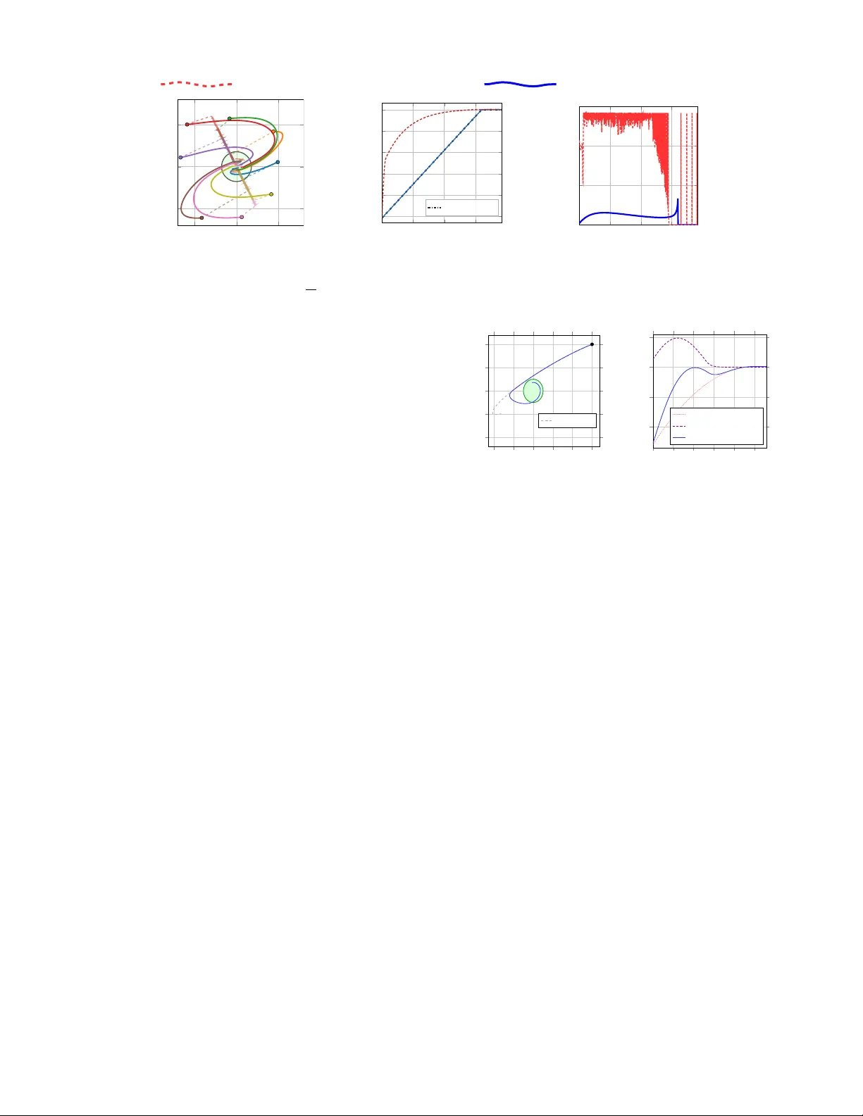
Constricting T ubes f or Pr escribed-Time Safe Contr ol Darshan Gadginmath Ahmed Allibhoy F abio Pasqualetti Abstract — W e propose a constricting Control Barrier Func- tion (CBF) framework for prescribed-time control of control- affine systems with input constraints. Given a system starting outside a target safe set, we construct a time-varying safety tube that shrinks from a r elaxed set containing the initial condition to the target set at a user-specified deadline. Any controller rendering this tube f orward in variant guarantees prescribed-time recovery by construction. The constriction schedule is bounded and tunable by design, in contrast to prescribed-time methods where contr ol effort diverges near the deadline. Feasibility under input constraints reduces to a single verifiable condition on the constriction rate, yielding a closed-form minimum recovery time as a function of control authority and initial violation. The framework imposes a single affine constraint per timestep regardless of state dimension, scaling to settings where grid-based reachability methods are intractable. W e v alidate on a 16-dimensional multi-agent system and a unicycle reach-a void problem, demonstrating prescribed- time recovery with bounded control effort. I . I N T R O D U C T I O N Driving a dynamical system into a desired set within a prescribed time is a recurring requirement where both timeliness and safety are critical. Applications such as satel- lite rendezvous under a mission deadline, or steering a robot into a goal region before a planning horizon expires require explicit prescribed-time control. The challenge is hardest when the system is nonlinear and subject to input constraints, a combination not well addressed by existing tools. Hamilton-Jacobi reachability [1], [2] provides formal guarantees but requires solving a PDE over the state space, scaling exponentially in dimension and precluding real-time synthesis. Control Barrier Functions (CBFs) [3] enable real- time synthesis via pointwise quadratic programs (QPs) and enforce forward in v ariance of a safe set, but are designed for systems that already satisfy the safety constraint. When the initial condition lies outside the target set, standard CBF conditions only achieve recov ery asymptotically . Prescribed- time and fixed-time methods attempt to address this gap, but share a common limitation. The con ver gence mechanism, whether a singular time-varying gain [4], a L yapuno v decay condition [5], or a slack v ariable [6], is implicit in the analysis rather than an e xplicit design parameter . As a result, it is difficult to bound control ef fort a priori or verify feasibility under input constraints at design time. In this paper , we propose a constricting tube framework that reduces the prescribed-time recovery problem to a for- D. Gadginmath is with the Department of Mechanical Engineering, Univ ersity of California at Ri verside, Ri verside, CA, 92521, USA. A. Al- libhoy and F . Pasqualetti are with the Department of Electrical Engineering and Computer Science at the Univ ersity of California at Irvine, Irvine, CA, 92697, USA. E-mail: dgadg001@ucr.edu , aallibho@uci.edu , fabiopas@uci.edu. ward in v ariance problem. Gi ven an initial condition outside the tar get set, we construct a time-varying tube that contains the initial state and collapses exactly to the tar get set at the deadline. The tube is parameterized by a designer-specified constriction schedule, bounded and tunable by construction, so that any controller rendering the tube forward inv ariant guarantees prescribed-time recovery . The constriction rate directly characterizes the worst-case control demand and ad- mits a closed-form characterization of the minimum deadline without requiring a L yapunov analysis or offline computa- tion. This yields a highly scalable frame work for prescribed- time control synthesis with con vergence certificates. Related work. The problem of stabilizing a target set has been studied from various angles. W e revie w the directions most rele vant to constrained prescribed-time stabilization. Hamilton-J acobi (HJ) reac hability . HJ reachability [1] provides formal safety and reachability guarantees via Hamilton-Jacobi-Isaacs PDEs solved backward in time. The backward reachable set (BRS) [7] is the set of initial condi- tions from which C can be reached at a prescribed terminal time T under optimal control, making this formulation most directly analogous to ours. Howe ver , solving the backward PDE requires discretizing the state space ov er a grid, and complexity scales as O ( M n ) with state dimension n and grid size M , limiting practical use to low-dimensional systems. The proposed frame work, by contrast, imposes a single af fine constraint per timestep and scales as O ( n ) , making it appli- cable to high-dimensional settings. Neural approximations such as DeepReach [8] extend HJ reachability to higher dimensions but require offline training and provide only probabilistic guarantees. The Control Barrier V alue Func- tion [9] recovers the maximal controlled-in variant set while admitting a QP-based controller , but does not provide an explicit mechanism for prescribed-time recov ery under input constraints. In contrast, the proposed framew ork imposes an affine constraint per timestep regardless of state dimension, admits an analytic feasibility certificate, and is demonstrated on a 16 -dimensional system, and higher in [10], where grid- based methods are computationally intractable. Pr escribed-time stabilization via scaling functions. A prominent line of work achie ves prescribed-time stabiliza- tion through a time-varying scaling function that diver ges unboundedly near the deadline [11], [12]. Fixed-time CLF methods [4] and their CBF extensions [6] enforce conv er- gence through Polyakov-type decay conditions. The CLF- based prescribed-time framew ork of [5] characterizes a feasibility re gion through global quadratic bounds on the CLF , but these constants are conservati ve and may not exist globally . Across all of these approaches, the control gain grows without bound as time reaches the deadline, and input constraints are handled through slack variables that may sacrifice the timing guarantee [6, Remark 5]. Pr escribed-time and fixed-time CBFs. Sev eral recent works modify the CBF condition with time-varying gains to enforce temporal guarantees. [13] combines fixed-time CBFs with MPC-based planning under input constraints, b ut does not explicitly characterize the minimum feasible dead- line. [14] achieves fixed-time con vergence for higher -order systems using a polynomial-in-time barrier , but does not account for input bounds and control effort grows near the deadline. [15] combines backstepping with a time-varying blow-up function for unknown dynamics, but relies on a class- K gain that di verges with time. A common limitation across these methods is that the conv ergence mechanism is implicit in the analysis, making it difficult to bound control effort a priori or v erify feasibility under input constraints. Our frame work makes the prescribed-time con ver gence mechanism explicit through a designer-specified constricting tube. Under input constraints, we deri ve feasibility con- straints for conv ergence under worst-case control demand. The framework also generalizes to stochastic systems, such as generati ve sampling models [10]. Contributions. The main contributions of this paper are: (i) A constricting CBF framew ork that guarantees prescribed-time recovery via forward inv ariance of a designer-specified safety tube, for any controller satisfying an affine constraint independent of state dimension. (ii) A feasibility analysis under input constraints, yielding a verifiable design-time condition on the constriction rate, a lo wer bound on the minimum recovery time. W e demonstrate the scalability of our framew ork on a 16- dimensional multi-agent system. W e further demonstrate its modularity to incorporate more constraints in a unicycle reach-av oid problem. In both cases, we show prescribed-time recov ery with bounded control. I I . C O N S T R I C T I N G C B F F R A M E W O R K A. Pr oblem formulation W e consider control-affine systems ˙ x = f ( x ) + g ( x ) u, (1) with state x ∈ R n , control u ∈ R m , and locally Lipschitz vector fields f : R n → R n and g : R n → R n × m . Let h : R n → R be a continuously differentiable function characterizing a target set C = { x : h ( x ) ≥ 0 } . Given a deadline T > 0 and an initial condition outside the target set x (0) / ∈ C , we seek a feedback control policy that solves the following problem. Problem 1 ( Prescribed-time control). Given system ( 1 ) with x (0) / ∈ C , synthesize a feedback policy u = κ ( x, t ) such that: (i) Prescribed-time recovery: x ( T ) ∈ C . (ii) Forward inv ariance: x ( t ) ∈ C for all t ≥ T . W e make the follo wing assumptions throughout the paper . Assumption 1 ( Control Barrier Function and Regularity ) . (i) h is a CBF for C with r espect to ( 1 ) : ther e exists an extended class- K function γ such that for all x ∈ R n sup u ∈ R m [ L f h ( x ) + L g h ( x ) u ] ≥ − γ ( h ( x )) , (2) (ii) L g h ( x )  = 0 for all x ∈ ∂ C . Assumption 1 (i) guarantees that C is controlled in variant, i.e., there always exists a control input keeping the system inside C once it has entered. Assumption 1 (ii) is a technical assumption required to ensure feasibility of the optimization- based feedback controller we introduce in the sequel. W e solve Problem 1 by defining a time-dependent relax- ation of the target set that constricts ov er time, so that any trajectory remaining inside the shrinking tube is driv en into C by the deadline. W ith this formulation, the problem reduces to maintaining forward in variance of the shrinking tube, as we describe ne xt. B. Constricting tubes for pr escribed-time contr ol W e begin by defining the constricting CBF , which aug- ments a gi ven CBF h with a time-dependent relaxation that encodes the desired conv ergence timeline. Definition 1 ( Constricting CBF ) . Given a CBF h for C and an initial condition x (0) , define the initial relaxation r 0 : = max  0 , − h ( x (0))  , (3) and the constricting CBF ˜ h : R n × [0 , T ] → R as ˜ h ( x, t ) = h ( x ) + r ( x (0) , t ) , (4) wher e r : R n × [0 , T ] → R ≥ 0 is C 1 in t and satisfies: (i) Initial containment: r ( x (0) , 0) = r 0 , (ii) T arget set recovery: r ( x (0) , T ) = 0 , (iii) Monotone constriction: ˙ r ( x (0) , t ) ≤ 0 for all t ∈ [0 , T ] . The constricting tube is the time-varying superlevel set ˜ C ( t ) = { x ∈ R n : ˜ h ( x, t ) ≥ 0 } , (5) satisfying x (0) ∈ ˜ C (0) and ˜ C ( T ) = C . The schedule r ( x (0) , t ) is parameterized by the initial condition and the entire schedule is determined once x (0) is fixed. The definition unifies two cases. When x (0) / ∈ C , we ha ve r 0 = − h ( x (0)) > 0 , and the relaxation inflates the target set so that x (0) ∈ ˜ C (0) . When x (0) ∈ C , we have r 0 = 0 , so r ( x (0) , t ) = 0 for all t and the tube reduces to ˜ C ( t ) = C , recov ering standard CBF-based forward in variance as a special case. The relaxation schedule, r ( x (0) , t ) , is a design choice independent of the system dynamics. Different schedules distribute the constriction differently over [0 , T ] . For exam- ple, the linear constriction r ( x (0) , t ) = r 0 (1 − t/T ) , with constant rate | ˙ r ( x (0) , t ) | = r 0 /T , is the simplest choice and admits sharp feasibility analysis (Theorem 2 ). Other examples include the exponential constriction r ( x (0) , t ) = x (0) x ( t ) x ( T ) C Constricting tub e ˜ C ( t ) Fig. 1. Geometry of the constricting tube framew ork. The initial condition x (0) lies outside the target set C = { x : h ( x ) ≥ 0 } . The schedule r ( x (0) , t ) inflates C into a tube ˜ C ( t ) = { x : h ( x ) + r ( x (0) , t ) ≥ 0 } containing x (0) at t = 0 . As r ( x (0) , t ) → 0 , the tube boundary constricts through the level sets of h until ˜ C ( T ) = C . Any controller rendering ˜ C ( t ) forward inv ariant guarantees x ( T ) ∈ C . r 0  e λ (1 − t/T ) − 1  / ( e λ − 1) , λ > 0 , and polynomial constric- tion r ( x (0) , t ) = r 0 (1 − t/T ) p . For exponential constriction, the tube contracts rapidly early , reducing peak control de- mand near t = T , whereas the polynomially constricted tube contracts slo wly at first and rapidly near the deadline. Solving problem 1 requires enforcing forward in v ariance of ˜ C ( t ) . If the trajectory ne ver leav es ˜ C ( t ) , then x ( T ) ∈ ˜ C ( T ) = C , thus achie ving the control objecti ve. W e formalize this in the following result. Theorem 1 ( Prescribed-time recov ery via tube inv ari- ance ) . Let ˜ h be a constricting CBF for C , with γ the extended class- K function fr om Assumption 1 (i). Then any locally Lipschitz feedback contr oller u = κ ( x, t ) satisfying L f h ( x ) + L g h ( x ) u + ˙ r ( x (0) , t ) ≥ − γ ( ˜ h ( x, t )) (6) for all ( x, t ) ∈ ˜ C ( t ) × [0 , T ] ensur es: (i) Prescribed-time recovery: x ( T ) ∈ C . (ii) Forward inv ariance: x ( t ) ∈ C for all t ≥ T . Proof . By Definition 1 (i), r ( x (0) , 0) = r 0 ≥ − h ( x (0)) , so ˜ h ( x (0) , 0) ≥ 0 and x (0) ∈ ˜ C (0) . Augment the state as z = ( x, t ) with dynamics ˙ z = [ f ( x ) + g ( x ) u, 1] ⊤ and define the space-time set ˜ S = { ( x, t ) : ˜ h ( x, t ) ≥ 0 } . On ∂ ˜ S , where ˜ h ( x, t ) = 0 , condition ( 6 ) reduces to L f h + L g h u + ˙ r ( x (0) , t ) ≥ 0 , which is the Nagumo tangency condition for ˜ S . By [16, Section 4.2.2], x (0) ∈ ˜ C (0) implies ˜ h ( x ( t ) , t ) ≥ 0 for all t ∈ [0 , T ] . At t = T , Definition 1 (ii) giv es r ( x (0) , T ) = 0 , so h ( x ( T )) = ˜ h ( x ( T ) , T ) ≥ 0 , proving (i). For t ≥ T , condition ( 6 ) with r ≡ 0 reduces to the standard CBF condition ( 2 ), and forward inv ariance of C follows from Assumption 1 (i) and [3], pro ving (ii). ■ The constriction rate ˙ r ( x (0) , t ) < 0 acts as an inward pressure beyond what is needed for forward inv ariance of a static set. This additional demand dri ves con ver gence. The faster the tube constricts, the harder the controller must push the state inward. Since r is C 1 on the compact interval [0 , T ] , ˙ r ( x (0) , t ) is bounded, and the additional demand is finite. A feedback controller can be synthesized by standard optimiza- tion techniques like in [3]. I I I . F E A S I B I L I T Y U N D E R I N P U T C O N S T R A I N T S W e synthesize here a feedback controller for input con- strained systems satisfying the hypotheses of Theorem 1 . W e assume the constraint is ∥ u ∥ ≤ u max , but our analysis generalizes to any constraint of the form u ∈ U where U is con ve x and compact. The proposed controller is κ ( x, t ) = argmin u ∈ R m J ( x, u, t ) s.t. L f h ( x ) + L g h ( x ) u + ˙ r ( x (0) , t ) ≥ − γ  ˜ h ( x, t )  , ∥ u ∥ ≤ u max . (7) When J is conv ex and quadratic in u , ( 7 ) is a conv ex program solv able in real time via standard solv ers. For t ≥ T , the constriction schedule satisfies ˙ r ( x (0) , t ) = 0 , and the program rev erts to the standard optimization-based safe controller with CBF constraints. Theorem 1 guarantees prescribed-time recov ery when- ev er the problem ( 7 ) is feasible. In the absence of input constraints, ( 6 ) is feasible for all ( x, t ) ∈ ˜ C × [0 , T ] by Assumption 1 (ii). Howe ver , the presence of input constraints fundamentally changes this picture. When ∥ u ∥ ≤ u max , the control authority av ailable to satisfy ( 6 ) is limited, and the constriction demand | ˙ r ( x (0) , t ) | may exceed what the actua- tors can deliver at certain states or times. In this setting, there is a tradeoff between the amount of control authority u max and the choice of deadline T : as u max decreases, one must tolerate a longer deadline in order to maintain feasibility . W e formalize this intuition next. T o choose a feasible deadline, it is crucial to v erify whether u max is large enough to meet the constriction demand | ˙ r ( x (0) , t ) | at every point on the tube. W e define the barrier authority to capture this idea. σ ( x ) : = max ∥ u ∥≤ u max ˙ h ( x, u ) = ∥ L g h ( x ) ∥ u max + L f h ( x ) . (8) The barrier authority , σ ( x ) , is the maximum rate that h can be increased at x ∈ R n . Example 1 ( Barrier authority for in verted pendulum ) . T o illustrate the geometry of the barrier authority , consider the contr olled simple pendulum ˙ x 1 = x 2 , ˙ x 2 = − sin x 1 + u, with CBF h ( x ) = c − ( x 1 − π ) 2 − x 2 2 , a ball of radius √ c ar ound the unstable upright equilibrium ( π , 0) . The barrier authority is σ ( x ) = 2 | x 2 | u max + 2 x 2  sin x 1 − ( x 1 − π )  . (9) F igur e 2 shows σ ( x ) over the domain [ π − 2 . 5 , π + 2 . 5] × [ − 2 . 5 , 2 . 5] for c = 0 . 01 and u max = 1 . 5 . The sign of σ depends only on x 1 : for each half-plane, σ factors as 2 x 2 · φ ( x 1 ) wher e φ ( x 1 ) = u max + sin x 1 − ( x 1 − π ) for x 2 > 0 , and − φ ( x 1 ) for x 2 < 0 , so the σ = 0 boundary is the vertical line x 1 = π ± 0 . 79 rad, independent of | x 2 | . The r e gion with a ne gative barrier authority (r ed) occupies two lobes. In both lobes, the drift L f h = 2 x 2 (sin x 1 − ( x 1 − π )) C π − 2 π − 1 π π +1 π +2 − 2 − 1 0 1 2 x 1 (angle) x 2 (angular velocity) − 4 − 2 0 2 4 σ ( x ) Fig. 2. Barrier authority σ ( x ) for the controlled pendulum targeting the upright equilibrium ( π , 0) (dot) with u max = 1 . 5 . Blue: σ > 0 ; red: σ < 0 . The red lobes correspond to states where the pendulum is displaced from upright and moving further away , so gravitational drift and velocity compound to reduce σ min . is larg e and negative: the pendulum is both displaced fr om upright (so gravity destabilizes) and moving away fr om it (so velocity compounds the drift), and together they exceed the available contr ol authority u max . If σ ( x ) ≤ 0 , e ven maximum control effort cannot increase h . At such points, the CBF condition will be infeasible. Let σ min be the worst-case barrier authority , σ min : = inf t ∈ [0 ,T ] x ∈ ˜ C ( t ) σ ( x ) . (10) The worst-case barrier authority captures the most demand- ing point on the tube, which is the state and time at which the system has the least capacity to push h upward, while the constriction schedule is still activ e. Feasibility of ( 7 ) at ( x, t ) ∈ ˜ C ( t ) × [0 , T ] reduces to comparing the constriction demand | ˙ r ( x (0) , t ) | against the local barrier authority σ ( x ) . When the constriction rate is too aggressive relati ve to the av ailable control authority , no admissible u can satisfy the CBF condition, and the program becomes infeasible. When σ min ≤ 0 , a longer deadline or a less aggressi ve constriction schedule may be required to restore feasibility . The follo wing result characterizes this tradeoff precisely , linking the deadline T , the constriction schedule r ( x (0) , t ) , and the bound u max in a single verifiable condition. Theorem 2 ( F easibility and minimum recovery time ) . Consider system ( 1 ) with the r elaxation schedule r ( x (0) , t ) and constricting CBF ( 4 ) . (i) Local feasibility: The pro gram ( 7 ) is feasible at ( x, t ) ∈ ˜ C ( t ) × [0 , T ] if and only if | ˙ r ( x (0) , t ) | ≤ σ ( x ) . (11) (ii) Global feasibility (linear schedule): F or the linear schedule r ( x (0) , t ) = r 0 (1 − t/T ) , pr ogram ( 7 ) is feasible for all ( x, t ) ∈ ˜ C ( t ) × [0 , T ] if and only if T ≥ T min : = r 0 σ min , (12) wher e r 0 is the initial violation ( 3 ) and σ min is the worst-case barrier authority ( 10 ) . Proof . On the boundary ∂ ˜ C ( t ) , ˜ h = 0 so γ ( ˜ h ) = 0 and the constraint ( 6 ) is most restrictiv e. In the interior, ˜ h > 0 so − γ ( ˜ h ) < 0 , and an y u satisfying the boundary condition also satisfies the interior condition. It is therefore suf ficient to analyze feasibility on ∂ ˜ C ( t ) . (i) Local feasibility . On ∂ ˜ C ( t ) , γ ( ˜ h ) = 0 and ( 6 ) reduces to L g h ( x ) u ≥ − L f h ( x ) + | ˙ r ( x (0) , t ) | , (13) where we used ˙ r ( x (0) , t ) ≤ 0 . The maximum of L g h ( x ) u ov er ∥ u ∥ ≤ u max is ∥ L g h ( x ) ∥ u max , achiev ed by align- ing u with L g h ( x ) ⊤ . A feasible u exists if and only if ∥ L g h ( x ) ∥ u max ≥ − L f h ( x ) + | ˙ r ( x (0) , t ) | , which rearranges to ( 11 ). Conv ersely , if | ˙ r ( x (0) , t ) | > σ ( x ) , then no u with ∥ u ∥ ≤ u max can satisfy ( 13 ), so ( 7 ) is infeasible. (ii) Global feasibility . For the linear schedule, | ˙ r ( x (0) , t ) | = r 0 /T is constant. Global feasibility requires the local condition ( 11 ) to hold for ev ery t ∈ [0 , T ] and all x ∈ ∂ ˜ C ( t ) , i.e., r 0 /T ≤ σ min . Rearranging giv es ( 12 ). Con versely , if T < T min then r 0 /T > σ min , so the local condition fails at the worst-case point on the tube boundary , and ( 7 ) is infeasible there. ■ The bound T min = r 0 /σ min depends on the initial con- dition through r 0 and, implicitly , through σ min since the tube boundary ∂ ˜ C ( t ) is initialized from x (0) . A larger initial violation r 0 or lo wer control authority σ min each increase T min , capturing the intuitive tradeof f. When u max = ∞ , σ min = ∞ and T min = 0 , consistent with the unconstrained case where any constriction rate is satisfiable. The analysis extends to any conv ex input constraint set U by replacing ∥ L g h ( x ) ∥ u max in ( 8 ) with max u ∈U L g h ( x ) u . Crucially , T min is computable before deploying the controller, provid- ing a design-time certificate for prescribed-time safety . The constriction schedule r ( x (0) , t ) giv es the designer a further handle beyond T . For a fixed T > T min , different schedules distribute the demand | ˙ r ( x (0) , t ) | dif ferently over [0 , T ] . The linear schedule imposes a constant pressure r 0 /T throughout; an exponential schedule concentrates the effort early , reducing peak demand near t = T . A polynomial schedule defers effort to ward the deadline. The local feasibil- ity condition ( 11 ) makes this tradeof f precise. The schedule is feasible at time t if and only if | ˙ r ( x (0) , t ) | ≤ σ ( x ) pointwise, so the designer can shape r ( x (0) , t ) to match the time-varying control authority of the system. Unlike methods that introduce slack variables and verify feasibility post-hoc [6], condition ( 11 ) is verifiable at design time directly from f , g , h , and u max , without solving the closed-loop system. For linear systems with a quadratic barrier , it admits a closed-form expression as follows. Corollary 3 ( Closed-form T min for linear systems ) . Con- sider the system ˙ x = Ax + B u , and h ( x ) = c − x ⊤ P x with c > 0 and P = P ⊤ ≻ 0 . The tube boundary ∂ ˜ C ( t ) = { x : x ⊤ P x = c + r ( x (0) , t ) } is an ellipsoid of radius ρ ( t ) = p c + r ( x (0) , t ) . On this boundary , the barrier authority ( 8 ) e valuates to σ ( x ) = 2  ∥ B ⊤ P x ∥ u max − x ⊤ P Ax  , (14) and its infimum over the tube horizon is ac hieved at t = T : σ min = 2 c  µ min u max − λ max ( P 1 / 2 AP − 1 / 2 )  , (15) wher e µ min := min ∥ P 1 / 2 v ∥ =1 ∥ B ⊤ P 1 / 2 v ∥ is the minimum input gain over the ellipsoid. The minimum reco very time is then T min = r 0 /σ min . W e provide an overvie w of the proof. The barrier au- thority for the linear system is ( 14 ). On the tube boundary x ⊤ P x = ρ ( t ) 2 , substitute x = ρ ( t ) P − 1 / 2 v with ∥ v ∥ = 1 . After substitution, σ ( x ) = 2 ρ ( t )  ∥ B ⊤ P 1 / 2 v ∥ u max − v ⊤ P 1 / 2 AP − 1 / 2 v  , which scales linearly in ρ ( t ) . Since ρ ( t ) is monotone decreasing, the infimum ov er the full tube is attained at t = T where ρ ( T ) = √ c , and minimizing over ∥ v ∥ = 1 yields ( 15 ). The expression ( 15 ) is positi ve if and only if µ min u max > λ max ( P 1 / 2 AP − 1 / 2 ) , i.e., the control authority exceeds the worst-case drift on the ellipsoid. If this condition fails, recovery in finite time is not possible. Remark 1 ( Extension to higher relativ e degree ) . When h has r elative de gr ee k > 1 with r espect to ( 1 ) , the frame work extends by combining the constricting barrier with the high- or der CBF construction of [17]: define ψ 0 ( x, t ) = h ( x ) + r ( x (0) , t ) and pr opagate thr ough the cascade ψ i = ˙ ψ i − 1 + γ i ( ψ i − 1 ) until the contr ol input appear s at or der k . The schedule r ( x (0) , · ) must be C k , and the constriction pressur e enters thr ough the k -th time derivative r ( k ) ( x (0) , t ) in the final constraint. A full tr eatment is left for futur e work. □ Remark 2 ( Relation to HJ reachability ) . The constricting schedule r ( x (0) , t ) is a conservative closed-form surr ogate for the backwar d reac hable set value function [7]. Both define a time-indexed family of le vel sets con ver ging to C at t = T , but our schedule yields an explicit feasibility certificate and optimization-based synthesis without offline computation. HJ-based methods pro vide globally optimal certificates but r equir e solving a PDE over a state-space grid, with exponentially scaling complexity , limiting appli- cability to low-dimensional systems [8]. Our constricting tube framework trades global optimality for tractability and global feasibility is guaranteed by the condition T ≥ T min , wher e T min ( 12 ) is computable analytically for structur ed systems (Cor ollary 3 ) or via con vex optimization. □ Remark 3 ( Recursiv e feasibility ) . Although Theorem 2 pr ovides conditions on pointwise feasibility at each ( x, t ) , it does not guarantee r ecursive feasibility . The r esulting tra- jectory may r each a configur ation fr om which no admissible contr ol satisfying ( 6 ) exists at a future time. However , for the specific systems considered in this work, feasibility holds for all time. Addressing r ecursive feasibility r equir es global r easoning o ver the full horizon, and r emains a direction for futur e work. □ I V . N U M E R I C A L E X P E R I M E N T S W e demonstrate our framework on a testbed of experi- ments to v alidate its scalability and practical use 1 . W e use γ ( ˜ h ) = α ˜ h , with α = 0 . 9 throughout. A. Prescribed-time r ecovery for a multi-agent system W e consider N = 8 decoupled agents, each governed by ˙ x i =  − 0 . 1 1 0 0 . 1  x i +  1 0 . 5  u i , i = 1 , . . . , N , (16) and scalar inputs u i ∈ R , | u i | ≤ u max = 2 . The full stacked system has state X = [ x ⊤ 1 , . . . , x ⊤ N ] ⊤ ∈ R 2 N and input U = [ u 1 , . . . , u N ] ⊤ ∈ R N , with dynamics ˙ X = A X + B U where A = blkdiag( A, . . . , A ) and B = blkdiag( B , . . . , B ) . W e use a joint barrier o ver the full 16D state, h ( X ) = c − ∥ X ∥ 2 (17) with c = 0 . 5 . All agents are initialized outside C , with individual norms ∥ x i (0) ∥ ranging from 1 . 93 to 3 . 20 . This experiment highlights the scalability of our frame- work. HJ reachability is computationally intractable over the full 16-dimensional state space, and methods like [11] require specific feedback structure, whereas our framew ork requires only the single eigenv alue computation ( 15 ). The block structure of A and B gi ves σ min = 2 c  ∥ B ∥ u max − λ max ( A )  ≈ 6 . 66 , (18) with initial violation r 0 = − h ( X 0 ) ≈ 50 . 66 , yielding T min = r 0 /σ min ≈ 4 . 57 s. W e set T = 6 . 4 s. W e apply the controller ( 7 ) o ver the full N -dimensional input U , with the linear schedule r ( t ) = max (0 , r 0 (1 − t/T )) , with J ( X , U, t ) = min U ∥ U ∥ 2 , so the controller applies only the minimum ef fort necessary to satisfy the constricting CBF constraint. W e compare against the prescribed-time method in [5]. The prescribed-time CLF V ( X , t ) = − h ( X ) /θ ( t ) 2 , θ ( t ) = 1 − t/T is used to synthesize U [5, Eq (30)]. Figure 3 sho ws (a) the phase portrait, (b) joint barrier h ( X ( t )) , and (c) aggregate control ef fort ∥ U ( t ) ∥ for both methods. Both methods successfully driv e the system into C by T . The state and control behavior , howe ver , differs funda- mentally . Our method maintains a modest, smoothly varying ∥ U ( t ) ∥ throughout the horizon, with a peak of ∥ U ∥ ≈ 3 . 66 , well below the saturation limit √ N u max ≈ 28 . 28 . The barrier h ( X ( t )) tracks the tube floor − r ( t ) closely , and the constricting schedule is the binding constraint. In contrast, the baseline [5] has high frequency variations and the control saturates persistently near √ N u max for approximately 70% of the horizon — a structural consequence of the gain sched- ule 1 /θ ( t ) that must div erge as t → T . Our method achieves the same prescribed-time guarantee with a fraction of the control effort, while respecting input constraints throughout. 1 Code repository: https://github.com/darshangm/ prescribed_time_control . Prescribed-time CLF [5] Constricting tube (ours) − 2 0 2 − 2 0 2 x 1 x 2 0 2 4 6 − 50 − 40 − 30 − 20 − 10 0 − r ( x (0) , t ) T ime (s) Barrier h ( x ( t )) 0 2 4 6 0 10 20 30 T ime (s) Control ef fort ∥ U ( t ) ∥ Fig. 3. Prescribed-time recovery for N = 8 agents with joint barrier h ( X ) = c − ∥ X ∥ 2 , c = 0 . 5 , and deadline T = 6 . 4 s. (Left) Phase portrait of agent trajectories under our method (solid) and [5] (dashed). The shaded disk is C . Both methods achieve prescribed-time recovery . (Middle) Joint barrier h ( X ( t )) . Our method tracks the constricting tube floor − r ( t ) (solid blue), entering C exactly at T . (Right) Control ef fort ∥ U ( t ) ∥ . The minimum norm controller stays well below the saturation limit √ N u max ≈ 28 . 28 , while [5] saturates persistently . B. Prescribed-time safety via HOCBF constricting tube W e apply the constricting tube framew ork to a system of relativ e degree 2, demonstrating the HOCBF extension of Remark 1 . The system is a planar double integrator ˙ p = v , ˙ v = u , with state x = ( p x , p y , v x , v y ) ⊤ , control u = ( u x , u y ) ⊤ , ∥ u ∥ ∞ ≤ u max = 2 m / s 2 , and initial condition x (0) = (3 , 2 , − 0 . 3 , − 0 . 1) ⊤ . The task is to driv e the position p = ( p x , p y ) into C = { x : ∥ p ∥ ≤ 0 . 5 } , by T = 25 s . The barrier h ( x ) = ϵ 2 − p 2 x − p 2 y satisfies L g h = 0 and has relative degree 2. W e use a C 2 quadratic schedule r ( x (0) , t ) = ( r 0 + δ )(1 − t/T ) 2 − δ , where r 0 = − h ( x (0)) = 12 . 75 and δ = ϵ 2 / 2 = 0 . 125 . The schedule satisfies r ( x (0) , 0) = r 0 and r ( x (0) , T ) = − δ , so the tube terminates δ inside C , guaranteeing h ( x ( T )) ≥ δ > 0 rather than merely h ( x ( T )) ≥ 0 . The HOCBF sequence is ψ 0 ( x, t ) = h ( x ) + r ( x (0) , t ) , (19) ψ 1 ( x, t ) = L f h + ˙ r ( x (0) , t ) + γ 1 ψ 0 , (20) with γ 1 = γ 2 = 0 . 9 . The condition ˙ ψ 1 + γ 2 ψ 1 ≥ 0 yields the QP constraint L 2 f h + L g L f h u + ¨ r ( x (0) , t ) + γ 1 ( L f h + ˙ r ( x (0) , t )) + γ 2 ψ 1 ≥ 0 . (21) W e demonstrate the use of our framew ork as a safety filter . A nominal PD controller u nom ( x ) = − k p p − k d v , k p = 0 . 01 , k d = 0 . 05 , (22) provides a stabilizing tendency toward the origin, and the HOCBF QP minimally deviates from it as follows: min u ∥ u − u nom ∥ 2 s.t. ( 21 ) , ∥ u ∥ ∞ ≤ u max . (23) The PD gains are deliberately slow: the nominal controller alone does not dri ve x into C by T = 25 s . The HOCBF constraint intervenes to enforce the deadline, with the con- stricting schedule pro viding the inward pressure. As seen in Figure 4 , the HOCBF controller achie ves ∥ p ( T ) ∥ = 0 . 36 m < ϵ with h ( x ( T )) = 0 . 121 > δ , confirming prescribed-time entry into the interior of C . The nominal controller does not enter C with time T as seen in Figure 4 (left), confirming that the HOCBF constraint is the mechanism responsible for the timing guarantee. − 2 − 1 0 1 2 3 − 2 − 1 0 1 2 x (0) Nominal p x (m) p y (m) 0 5 10 15 20 25 − 10 − 5 0 5 − r ( t ) (tube floor) ψ 1 ( x, t ) h ( x ( t )) — HOCBF T ime (s) ψ 0 , h ( x ) Fig. 4. Higher order constricting tubes for the double integrator with relativ e degree 2, T = 25 s . (Left) Position trajectory: the HOCBF controller (blue) enters C by T ; the nominal PD controller (red) does not. (b) Barrier values ψ 0 ( x, t ) (tube) and h ( x ( t )) (target set): ψ 0 ≥ 0 is maintained throughout and h ( x ( T )) ≥ δ > 0 at the deadline. C. Prescribed-time r each-avoid planning for a unicycle W e demonstrate the constricting tube framework in a trajectory planning setting where a nonlinear unicycle must reach a tar get region by a deadline while av oiding an obstacle that lies directly on the straight-line path to the target. W e embed the constricting tube and obstacle av oid- ance as hard path constraints in a model predictiv e control problem, solved online with IPOPT via CasADi. Let x = ( p x , p y , θ ) ⊤ ∈ R 2 × S 1 denote the position and heading of the unicycle, with control u = ( v, ω ) ⊤ , ˙ p x = v cos θ, ˙ p y = v sin θ, ˙ θ = ω . (24) Controls are bounded by | v | ≤ v max = 1 . 5 m / s and | ω | ≤ ω max = 2 . 0 rad / s . The unicycle starts at x (0) = (4 . 0 , 3 . 0 , θ 0 ) ⊤ with θ 0 = atan2( − 3 , − 4) , pointing directly tow ard the origin at distance ∥ p (0) ∥ = 5 m . The constricting r each barrier targets the ball C 1 = { x : h ( x ) ≥ 0 } with h ( x ) = ϵ 2 − p 2 x − p 2 y , ϵ = 0 . 5 m . (25) The static avoidance barrier keeps the unicycle outside a circular obstacle of radius ρ = 0 . 6 m centered at c = (2 . 0 , 1 . 5) ⊤ , which lies on the path from x (0) to the origin: h obs ( x ) = ∥ p − c ∥ 2 − ρ 2 . (26) − 1 0 1 2 3 4 − 1 0 1 2 3 4 x (0) p x p y 0 5 10 15 20 − 20 − 10 0 − r ( x (0) , t ) h (T arget set CBF) h obs (Avoidance CBF) T ime Fig. 5. Prescribed-time reach-avoid planning with the unicycle. (Left) The planner navigates around the obstacle (red) and enters the target set (green) by the deadline. (Right) Barrier value vs. time: Prescribed-time reach CBF h ( x ( t )) (blue, solid) rises from − 24 . 75 to +0 . 233 > δ at t = T , staying above the constricting tube floor − r ( x (0) , t ) (blue, dotted) throughout. Collision av oidance CBF h obs ( x ( t )) (red, dash-dotted) stays positive. W e have h 1 ( x (0)) = − 24 . 75 < 0 and h obs ( x (0)) = 5 . 89 > 0 , so the unic ycle starts outside the target but safely clear of the obstacle. W e use the quadratic schedule r ( x (0) , t ) = r 0  1 − t T  2 , (27) with r 0 = − h ( x (0)) = 24 . 75 , and deadline T = 20 s . At each planning instance t , we solve the following optimal control problem o ver the horizon [ t, t + S ] with S = 1 . 5 s : min u ( · ) Z t + S t ∥ u ( τ ) ∥ 2 d τ + β ∥ p ( t + S ) ∥ 2 s . t . ˙ x ( τ ) = f ( x ( τ )) + g  x ( τ ) , u ( x ( τ ) , τ )  , h  x ( τ )  + r ( x (0) , τ ) ≥ 0 , h obs  x ( τ )  ≥ 0 , | v ( τ ) | ≤ v max , | ω ( τ ) | ≤ ω max , ∀ τ ∈ [ t, t + S ] . Here f ( x ) + g ( x, u ) denotes the unicycle dynamics ( 24 ) and β = 10 penalizes the terminal distance to the origin. The con- stricting tube constraint ev aluates r ( τ ) at time τ ∈ [ t, t + S ] , so the planner is aware of the tightening schedule throughout the horizon and proactively plans the obstacle detour with the remaining time b udget in mind. The continuous-time problem is solved using Euler discretization d t = 0 . 005 s, and the optimal control over the first interval is applied as the horizon advances. The planner safely navigates around the obstacle, maintaining h obs ( x ( τ )) ≥ 0 at all times, and achiev es h ( x ( T )) = +0 . 233 > δ = 0 . 2 , placing the unicycle at ∥ p ( T ) ∥ = 0 . 13 m strictly inside C 1 at the deadline. Figure 5 illustrates the trajectory and barrier histories. V . C O N C L U S I O N W e introduced a constricting CBF framew ork that reduces prescribed-time recovery to a forward in variance problem via a designer-specified constricting tube. The framew ork yields a single af fine constraint independent of the state dimension, with feasibility conditions verifiable at design time. Control effort is bounded throughout the horizon by construction, in contrast to prescribed-time methods where gains must div erge as the deadline approaches. V alidation on a 16- dimensional multi-agent system demonstrates scalability of the frame work, with peak control effort well below the saturation limit. A unic ycle reach-avoid problem further demonstrates the modularity of the framework to incorporate multiple simultaneous constraints. Future directions include robustness to disturbances, optimal schedule design, and recursiv e feasibility guarantees under input constraints. R E F E R E N C E S [1] S. Bansal, M. Chen, S. Herbert, and C. J. T omlin. Hamilton-jacobi reachability: A brief overview and recent advances. In IEEE Conf. on Decision and Contr ol , pages 2242–2253, Melbourne, Australia, 2017. [2] I. M. Mitchell, A. M. Bayen, and C. J. T omlin. A time-dependent hamilton-jacobi formulation of reachable sets for continuous dynamic games. IEEE T ransactions on Automatic Contr ol , 50(7):947–957, 2005. [3] A. D. Ames, S. Coogan, M. Egerstedt, G. Notomista, K. Sreenath, and P . T abuada. Control barrier functions: Theory and applications. In Eur opean Control Confer ence , pages 3420–3431, Naples, Italy , 2019. [4] A. Polyako v . Nonlinear feedback design for fixed-time stabilization of linear control systems. IEEE T ransactions on Automatic Control , 57(8):2106–2110, 2011. [5] K. Garg, E. Arabi, and D. Panagou. Prescribed-time con vergence with input constraints: A control lyapunov function based approach. In American Contr ol Conference , pages 962–967, Denv er, Colorado, 2020. [6] K. Garg and D. Panagou. Robust control barrier and control lyapunov functions with fixed-time conv ergence guarantees. In American Con- tr ol Conference , pages 2292–2297, New Orleans, Louisiana, 2021. [7] J. F . Fisac, M. Chen, C. J. T omlin, and S. S. Sastry . Reach- av oid problems with time-v arying dynamics, tar gets and constraints. In International Conference on Hybrid Systems: Computation and Contr ol , pages 11–20, Seattle, W ashington, 2015. [8] S. Bansal and C. J. T omlin. Deepreach: A deep learning approach to high-dimensional reachability . In IEEE Int. Conf. on Robotics and Automation , pages 1817–1824, Xi’an, China, 2021. [9] J. J. Choi, D. Lee, K. Sreenath, C. J. T omlin, and S. L. Herbert. Robust control barrier–value functions for safety-critical control. In IEEE Conf. on Decision and Control , pages 6814–6821, Austin, T exas, 2021. [10] D. Gadginmath, A. Allibhoy , and F . P asqualetti. Provably safe generativ e sampling with constricting barrier functions. arXiv preprint arXiv:2602.21429 , 2026. [11] Y . Song, Y . W ang, J. Holloway , and M. Krstic. Time-v arying feedback for regulation of normal-form nonlinear systems in prescribed finite time. Automatica , 83:243–251, 2017. [12] W . Li and M. Krstic. Prescribed-time output-feedback control of stochastic nonlinear systems. IEEE T ransactions on Automatic Con- tr ol , 68(3):1431–1446, 2023. [13] K. Garg, R. K. Cosner, U. Rosolia, A. D. Ames, and D. Panagou. Multi-rate control design under input constraints via fixed-time barrier functions. IEEE Control Systems Letters , 6:608–613, 2021. [14] Janani S. K. and S. K olathaya. Fixed time con vergence guar- antees for higher order control barrier functions. arXiv preprint arXiv:2507.13888 , 2025. [15] T .-Y . Huang, S. Zhang, X. Dai, A. Capone, V . T odorovski, S. Sos- nowski, and S. Hirche. Learning-based prescribed-time safety for control of unknown systems with control barrier functions. IEEE Contr ol Systems Letters , 8:1817–1822, 2024. [16] F . Blanchini and S. Miani. Set-theoretic methods in contr ol , v olume 78. Springer , 2008. [17] W . Xiao and C. Belta. High-order control barrier functions. IEEE T ransactions on Automatic Contr ol , 67(7):3655–3662, 2021.