Koopman Lifted Finite Memory Identification via Truncated Grunwald Letnikov Kernels

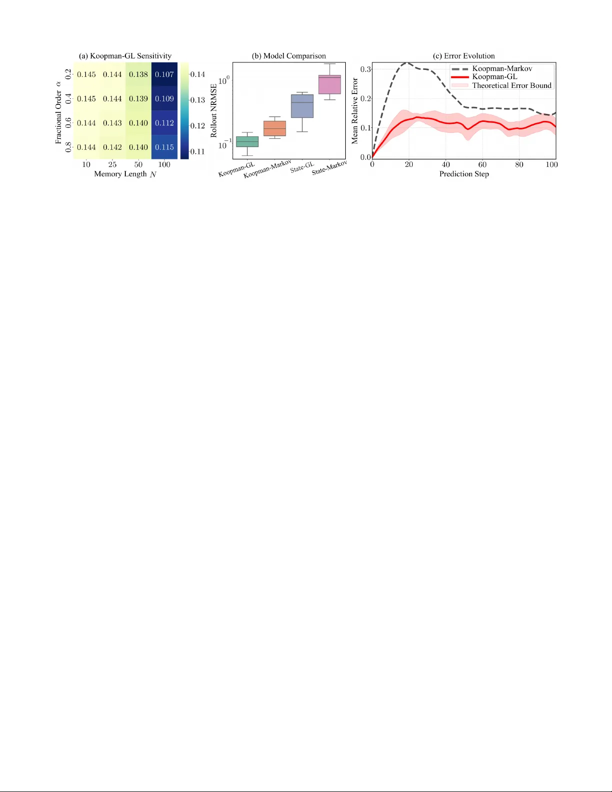
K oopman-Lifted Finite-Memory Identification via T runcated Gr ¨ unwald–Letniko v K ernels Navid Mojahed 1 ∗ , Mahdis Rabbani 1 ∗ , and Shima Nazari 1 Abstract — W e propose a data-driven linear modeling frame- work for controlled nonlinear her editary systems that combines Koopman lifting with a truncated Gr ¨ unwald–Letnikov memory term. The key idea is to model nonlinear state dependence through a lifted observable r epresentation while imposing his- tory dependence directly in the lifted coordinates through fixed fractional-difference weights. This preserves linearity in the lifted state-transition and input matrices, yielding a memory- compensated regression that can be identified fr om input–state data by least squares and extending standard Koopman-based identification beyond the Markovian setting. W e further derive an equivalent augmented Markovian realization by stacking a finite window of lifted states, thereby rewriting the finite- memory recursion as a standard discrete–time linear state– space model. Numerical experiments on a nonlinear heredi- tary benchmark with a non-Gr ¨ unwald–Letnikov Pr ony-series ground-truth kernel demonstrate improv ed multi-step open- loop prediction accuracy relative to memoryless Koopman and non-lifted state-space baselines. I . I N T RO D U C T I O N Many engineering systems exhibit hereditary dynamics, in which the present state depends not only on the current state and control input, but also on past values. Such behavior appears in a broad range of applications, including dielectric phenomena, viscoelastic and compliant mechanical systems, and interaction-rich robotic settings with friction, hysteresis, or relaxation effects [1]–[5]. Fractional-order models hav e gained significant attention as a powerful framework for describing these processes, since they capture long-memory temporal correlations that are difficult to represent accurately using low-order integer-order models [1], [2]. Although fractional-order modeling applies to both linear and nonlinear systems [6], [7], this work focuses on the non- linear setting, where hereditary effects and state-dependent nonlinearities must be addressed simultaneously . In such sys- tems, memoryless integer -order models can be inadequate, especially in long-horizon prediction and optimization-based control, where small one-step model errors can accumulate and degrade closed-loop performance [1], [2], [6], [8]. Classical simplifications for nonlinear systems, such as operating-point linearization and T aylor -series approxima- tions, are often local in nature and tend to lose accu- racy as the system mo ves aw ay from the operating regime [9]. Koopman-based methods offer an alternativ e by lift- ing the state to a higher-dimensional space of observ ables and seeking an approximately linear predictor there [10], ∗ These authors contributed equally to this work. 1 The authors are with the Department of Mechanical and Aerospace Engineering, Univ ersity of California, Davis, CA 95616, USA. nmojahed@ucdavis.edu, [11]. Through data-driven identification procedures such as DMD/EDMD [12]–[14], these methods have attracted in- creasing attention for nonlinear prediction and control. Howe ver , standard K oopman identification pipelines are typically formulated as one-step Markovian predictors in the lifted space [8], which can lead to substantial plant– model mismatch when applied to hereditary or fractional- order systems. Some recent w orks combine K oopman-based plant representations with fractional-order controllers [15]– [17]. While such approaches can be effecti ve in practice, they do not directly address the identification of a lifted predictor for a plant whose dynamics are themselves in- trinsically hereditary . This moti vates the study of K oopman identification for genuinely fractional-order dynamics. Sev eral recent directions hav e begun to relax the purely Markovian viewpoint in K oopman modeling. One line of work uses delay or history augmentation to obtain approxi- mately Marko vian representations in expanded coordinates [18]–[20]. Another incorporates memory directly into the ev olution model, as in dynamic mode decomposition with memory and related fractional variants [21]. More recent de- velopments include explicit non-Marko vian closures inspired by Mori–Zwanzig theory and latent memory corrections [22], [23], as well as operator-theoretic settings defined on trajectories or signals rather than instantaneous states [24]. Despite these advances, the problem of learning a structured, control-friendly lifted predictor for intrinsically hereditary dynamics remains largely open. Although these directions are notable, they do not fully resolve the identification problem considered here: learning a structured, control-friendly lifted predictor for a plant whose dynamics are intrinsically non-Marko vian. This paper adopts that hereditary viewpoint explicitly . Rather than starting from a memoryless plant and enriching the observable space with delays, we assume from the outset that the plant is history-dependent. K oopman lifting is used to capture nonlinear state dependence, while memory is modeled directly in the lifted coordinates through a trun- cated Gr ¨ unwald–Letniko v (GL) representation. Because GL discretizations express fractional differinte grals as weighted sums of past samples, they induce a structured con volu- tional memory form that is compatible with finite-memory approximation, lifted regression, and history stacking [6], [25]. This yields a finite-memory lifted predictor that can be re written, by stacking a finite window of lifted states, as a standard one-step model on an augmented state. In this way , the proposed framew ork connects K oopman-based learning with finite-memory hereditary approximation while remaining compatible with data-driv en prediction and control [6], [26]. The main contributions of this paper are as follo ws: 1) W e propose a Koopman-compatible finite-memory modeling frame work for nonlinear hereditary systems, in which memory is modeled explicitly in lifted coor- dinates through a truncated Gr ¨ unwald–Letniko v term rather than being ignored under a Marko vian lifted predictor . 2) W e deriv e a memory-compensated identification re- formulation that remains linear in the lifted state- transition and input matrices, enabling least-squares learning of the finite-memory lifted model directly from input–state data. 3) W e derive an exact augmented Marko vian realization by stacking a finite lifted history , thereby con vert- ing the non-Markovian finite-memory recursion into a standard one-step state-space model. 4) W e quantify the effect of finite-memory approximation through bounds on kernel mismatch and neglected memory tail, and validate the overall framework on a nonlinear hereditary benchmark with a non-GL ground-truth kernel. I I . P RO B L E M S T A T E M E N T & B A C K G RO U N D W e consider a discrete-time nonlinear hereditary system of the form x k +1 = f ( x k , u k ) + J ref X j =1 h j g ( x k +1 − j ) + η k , k ∈ N , (1) where x k ∈ R n and u k ∈ R m denote the state and control input, respectively , f : R n × R m → R n represents the instantaneous state-update map, g : R n → R n describes the contribution of past states to the current evolution, { h j } J ref j =1 ⊂ R defines the memory k ernel gi ven a memory length J ref ∈ N , and η k ∈ R n collects exogenous distur- bances and model mismatch. Unlike a Markovian system, the e volution in (1) depends not only on the current state and input, b ut also on the history of past states through the con volution term. T o obtain a linear predictor in lifted coordinates of the nonlinear dynamics in (1), we adopt a finite-dimensional K oopman lifting in the spirit of EDMD/EDMDc [13]. Specif- ically , we define the lifted state as z k := ψ ( x k ) ∈ R p , (2) where the vector-v alued observable map ψ ( · ) is chosen as ψ ( x ) =   1 x ϕ ( x )   , ϕ : R n → R p ϕ , p = 1 + n + p ϕ . (3) Here, ϕ ( x ) denotes a user-chosen collection of nonlinear observable functions of the state, used to enrich the lifted representation be yond constant and linear terms. W ith this construction, the original state remains an exact linear read- out of the lifted coordinates: x k = C z k , C :=  0 I n 0 p ϕ  ∈ R n × p . (4) In standard EDMDc, one seeks lifted state-transition ma- trix ¯ A ∈ R p × p and lifted input matrix ¯ B ∈ R p × m such that the lifted dynamics are approximated by the Marko vian predictor z k +1 = ¯ Az k + ¯ B u k + r k , (5) where r k ∈ R p captures finite-dimensional closure error and other unmodeled effects. The matrices ( ¯ A, ¯ B ) are typically identified from snapshot data through a least-squares regres- sion on lifted state-input pairs. Model (5), howe ver , remains Markovian in the lifted coordinates and therefore does not explicitly account for the hereditary effects in (1). This motiv ates the memory- augmented lifted model de veloped next. I I I . K O O P M A N – G L F I N I T E - M E M O RY I D E N T I FI C A T I O N T o address this limitation while preserving a regression form in the lifted state-transition and input matrices, we in- troduce a finite-memory Gr ¨ unwald–Letniko v (GL) correction in the lifted coordinates. For a fractional order α ∈ (0 , 1) , the discrete-time GL fractional dif ference of a lifted sequence { z k } is defined as [6], [27] (∆ α z ) k +1 := k +1 X j =0 w j ( α ) z k +1 − j , (6) where the GL coef ficients are given by w j ( α ) = ( − 1) j  α j  , j ≥ 0 , (7) with w 0 ( α ) = 1 , and satisfy the recursion w j ( α ) = − w j − 1 ( α ) α − ( j − 1) j , j ≥ 1 . (8) Any kno wn constant scaling, such as ∆ t − α in a fractional- deriv ative discretization, can be absorbed into the coef ficients w j ( α ) . Giv en a truncated memory length N ∈ N , N ≤ J ref , a fractional order α ∈ (0 , 1) , and an initial lifted history { z 0 , z 1 , . . . , z N − 1 } , we propose the finite-memory lifted model z k +1 = ¯ Az k + ¯ B u k − N X j =1 w j ( α ) z k +1 − j + d k , k ≥ N − 1 , (9) where d k ∈ R p collects the residual ef fects not captured by the imposed finite-memory GL structure, including finite- dimensional K oopman closure error, finite-memory trunca- tion error , and possible mismatch between the true hereditary kernel and the adopted GL kernel. Model (9) may therefore be vie wed as a structured hered- itary correction of the Markovian lifted predictor (5): the matrices ( ¯ A, ¯ B ) capture the instantaneous lifted dynamics, while the GL con volution term accounts for memory effects through a finite history of lifted states. A. Memory-Compensated Re gr ession Suppose a sequence of lifted snapshots and inputs is av ailable over a data horizon T , together with the initial lifted history { z 0 , . . . , z N − 1 } , and let the memory length satisfy N < T . For each k = N − 1 , . . . , T − 1 , define the memory-compensated target y k := z k +1 + N X j =1 w j ( α ) z k +1 − j ∈ R p . (10) Substituting (9) into (10) yields y k = ¯ Az k + ¯ B u k + d k . (11) Thus, after moving the kno wn GL memory term to the left- hand side, the hereditary lifted dynamics reduce to a linear regression in the current lifted state and input. For identification, stack the data as Y =  y N − 1 · · · y T − 1  , Z =  z N − 1 · · · z T − 1  , U =  u N − 1 · · · u T − 1  , D =  d N − 1 · · · d T − 1  . Then (11) can be written compactly as Y = Θ ⋆ Ω+ D , Ω :=  Z U  , Θ ⋆ :=  ¯ A ¯ B  . (12) Giv en (12), identification of the lifted state-transition and input matrices reduces to the least-squares problem ˆ Θ ∈ arg min Θ ∥ Y − ΘΩ ∥ 2 F . (13) Under a standard excitation condition, namely that Ω has full ro w rank, problem (13) admits a unique least-squares minimizer with the usual closed-form expression ˆ Θ = Y Ω † = Y Ω ⊤ (ΩΩ ⊤ ) − 1 . The following result characterizes the resulting identification error in terms of the aggregate disturbance matrix D . Theor em 1 (Identification err or bound): Suppose Ω has full row rank and satisfies ΩΩ ⊤ ⪰ µI p + m for some µ > 0 . If the stacked regression satisfies (12), then the least-squares estimator ˆ Θ = Y Ω † obeys ˆ Θ − Θ ⋆ = D Ω † , (14) and therefore ∥ ˆ Θ − Θ ⋆ ∥ F ≤ ∥ D ∥ F ∥ Ω † ∥ 2 ≤ ∥ D ∥ F √ µ . (15) Pr oof: Since Ω has full row rank, the least-squares minimizer is uniquely giv en by ˆ Θ = Y Ω † . Substituting (12) yields ˆ Θ = (Θ ⋆ Ω + D )Ω † = Θ ⋆ (ΩΩ † ) + D Ω † . Because Ω has full ro w rank, ΩΩ † = I , which proves (14). T aking Frobenius norms and using submultiplicativity gi ves ∥ ˆ Θ − Θ ⋆ ∥ F ≤ ∥ D ∥ F ∥ Ω † ∥ 2 . Finally , ΩΩ ⊤ ⪰ µI implies σ min (Ω) ≥ √ µ and hence ∥ Ω † ∥ 2 = 1 σ min (Ω) ≤ 1 √ µ , which proves (15). It is note worthy that in practice, the stacked quantities are formed from measured lifted snapshots ˜ z k = ψ ( ˜ x k ) ; accordingly , the targets are computed as ˜ y k := ˜ z k +1 + N X j =1 w j ( α ) ˜ z k +1 − j , and the resulting lifting and measurement effects are ab- sorbed into the disturbance term D . I V . F I N I T E - M E M O RY A P P ROX I M AT I O N E R RO R Theorem 1 shows that the identification error is controlled by the aggregate disturbance matrix D . W e no w make one important component of this disturbance explicit, namely the approximation error induced by replacing an infinite-memory kernel with the truncated GL kernel used in (9). The main contribution of this section is an explicit decomposition of this error into a retained-lag kernel-mismatch term and a neglected-tail term, followed by bounds that rev eal ho w the approximation depends on the memory length N and the fractional order α . T o expose this approximation error , consider the reference lifted model z k +1 = ¯ Az k + ¯ B u k − k +1 X j =1 c ⋆ j z k +1 − j + ξ k , k ≥ 0 , (16) where { c ⋆ j } j ≥ 1 is a scalar reference memory kernel shared across the lifted coordinates, and ξ k ∈ R p collects e xoge- nous disturbances and residual lifted-model mismatch. The proposed predictor (9) approximates the reference kernel { c ⋆ j } j ≥ 1 by a truncated GL kernel, i.e., by taking w j ( α ) for j = 1 , . . . , N and neglecting all lags beyond N . Comparing (16) with (9) gi ves, for all k ≥ N − 1 , d k = N X j =1  w j ( α ) − c ⋆ j  z k +1 − j − k +1 X j = N +1 c ⋆ j z k +1 − j + ξ k . (17) Thus, the additiv e disturbance consists of three contributions: (i) a kernel-mismatch term over the retained lags j = 1 , . . . , N , (ii) a tail term due to ne glecting lags beyond N , and (iii) the residual term ξ k . This decomposition is particularly rele vant for the numer- ical experiments in Section VI, where the reference kernel is chosen from a non-GL family (Prony series). In that case, the retained-lag mismatch term in (17) generally does not v anish, ev en if the GL surrogate yields good predicti ve performance. Define ε N ( α ; c ⋆ ) := N X j =1   c ⋆ j − w j ( α )   + ∞ X j = N +1 | c ⋆ j | . (18) Theor em 2 (F inite-memory modeling error bound): Assume ∥ z k ∥ 2 ≤ M z for all k = 0 , . . . , T . Then, for e very k = N − 1 , . . . , T − 1 , the disturbance in (17) satisfies ∥ d k ∥ 2 ≤ M z ε N ( α ; c ⋆ ) + ∥ ξ k ∥ 2 . (19) In particular, if ∥ ξ k ∥ 2 ≤ ¯ ξ , then ∥ d k ∥ 2 ≤ M z ε N ( α ; c ⋆ ) + ¯ ξ . (20) Pr oof: From (17), the triangle inequality and the uniform bound ∥ z ℓ ∥ 2 ≤ M z giv e ∥ d k ∥ 2 ≤ M z N X j =1   w j ( α ) − c ⋆ j   | {z } retained-lag mismatch + M z k +1 X j = N +1 | c ⋆ j | | {z } neglected tail + ∥ ξ k ∥ 2 . Since P k +1 j = N +1 | c ⋆ j | ≤ P ∞ j = N +1 | c ⋆ j | , the claim immediately follows from (18). W e next specialize to the GL coef ficients and quantify the decay of their tail. This yields an explicit truncation rate when the reference kernel is itself GL, or when the GL tail is used as a structured surrogate for long-memory effects. Lemma 1 (Decay and tail mass of GL coefficients): For any fixed α ∈ (0 , 1) , there exists a constant C α > 0 such that | w j ( α ) | ≤ C α j − (1+ α ) , ∀ j ≥ 1 . (21) Consequently , the GL tail mass δ N ( α ) satisfies δ N ( α ) := ∞ X j = N +1 | w j ( α ) | ≤ C α α N − α . Pr oof: The result follows from standard asymptotic properties of the generalized binomial coefficients defin- ing the GL weights. In particular, the coefficients admit a Gamma-function representation, from which one obtains the polynomial decay | w j ( α ) | = O  j − (1+ α )  . The bound on the tail mass then follows by summing this decay estimate over j ≥ N + 1 and applying a comparison with the corresponding improper integral. The full deriv ation is omitted due to space constraints. Cor ollary 1 (Pur e truncation bound for exact GL kernel): Suppose the reference kernel in (16) is exactly GL, i.e., c ⋆ j = w j ( α ) , ∀ j ≥ 1 . Then the retained-lag mismatch term in (17) v anishes, and for all k = N − 1 , . . . , T − 1 , ∥ d k ∥ 2 ≤ M z δ N ( α ) + ∥ ξ k ∥ 2 . (22) In particular, Lemma 1 implies ∥ d k ∥ 2 ≤ M z C α α N − α + ∥ ξ k ∥ 2 . (23) Pr oof: If c ⋆ j = w j ( α ) for all j ≥ 1 , then (18) reduces to ε N ( α ; c ⋆ ) = ∞ X j = N +1 | w j ( α ) | = δ N ( α ) . The result follows immediately from Theorem 2 and Lemma 1. V . E Q U I V A L E N T A U G M E N T E D M A R K OV I A N R E A L I Z A T I O N The identified K oopman–GL model (9) is finite-memory and therefore non-Markovian, i.e., the update of the next lifted state depends on the current lifted state, the current input, and a finite history of past lifted states. T o enable the use of standard one-step state-space tools for analysis and control design, we now deri ve an equiv alent Markovian realization by augmenting the lifted state with an N -sample history stack. This exact augmentation constitutes the second main contribution of the paper . Starting from the finite-memory lifted model (9), define the augmented lifted state and disturbance as z aug k :=      z k z k − 1 . . . z k − N +1      ∈ R pN , d aug k :=      d k 0 . . . 0      ∈ R pN . (24) The augmented state stores the most recent N lifted states, while all lifting, truncation, and exogenous disturbance ef- fects enter only through the first block. W ith this construction, the N -step recursion (9) is equiv- alently represented by the one-step Markovian system z aug k +1 = A aug z aug k + B aug u k + d aug k , k ≥ N − 1 , (25) where the augmented matrices A aug ∈ R pN × pN and B aug ∈ R pN × m hav e the block companion form A aug =         ¯ A − w 1 ( α ) I p − w 2 ( α ) I p · · · − w N ( α ) I p I p 0 · · · 0 0 I p . . . . . . . . . . . . . . . 0 0 · · · I p 0         , B aug =      ¯ B 0 . . . 0      . (26) The GL structure enters only through the scalar coefficients { w j ( α ) } N j =1 in the first block ro w of A aug . Consequently , the augmentation preserves the structured low-parameter form of the identified finite-memory model, rather than introducing a fully free matrix-v alued lag representation. Theor em 3 (Exact augmented Marko vian r ealization): Consider the finite-memory recursion (9) and the augmented system (25)–(26), dri ven by the same input sequence { u k } . If z aug N − 1 =  z ⊤ N − 1 , z ⊤ N − 2 , . . . , z ⊤ 0  ⊤ , (27) then, for all k ≥ N − 1 , z aug k =  z ⊤ k , z ⊤ k − 1 , . . . , z ⊤ k − N +1  ⊤ . (28) Hence, the first block of z aug k equals z k , and (9) is exactly equiv alent to the one-step Markovian realization (25). Pr oof: The result follows by induction on k ≥ N − 1 . The initialization (27) establishes (28) at k = N − 1 . Assume that (28) holds at time k . Then the first block row of (25) giv es z (1) k +1 =  ¯ A − w 1 ( α ) I p  z k − N X j =2 w j ( α ) z k +1 − j + ¯ B u k + d k , which is e xactly (9). Hence, the first block of z aug k +1 equals z k +1 . For the remaining blocks, the lower block rows of A aug implement the deterministic shift z ( i ) k +1 = z ( i − 1) k , i = 2 , . . . , N . Using the induction hypothesis, these blocks become z k , z k − 1 , . . . , z k − N +2 , respectively . Hence, z aug k +1 =  z ⊤ k +1 , z ⊤ k , . . . , z ⊤ k − N +2  ⊤ , which is exactly (28) at time k + 1 . This completes the induction. V I . N U M E R I C A L E X P E R I M E N T S W e ev aluate the proposed Koopman–GL framework on a controlled nonlinear hereditary benchmark. The ground- truth system is a two-dimensional nonlinear map with state x = [ x 1 , x 2 ] ⊤ and scalar input u , generated according to (1) with J ref = 400 . The instantaneous dynamics are f 1 ( x, u ) = 0 . 90 x 1 + 0 . 10 sin( x 2 ) + 0 . 10 u, f 2 ( x, u ) = 0 . 85 x 2 + 0 . 08 cos( x 1 ) + 0 . 05 x 2 1 + 0 . 05 u, and the hereditary contribution is defined by g ( x ) = [tanh( x 1 ); 0] , so that memory acts only on the first state component. The memory kernel is chosen as the Prony series h j = a 1 ρ j 1 + a 2 ρ j 2 , j = 1 , . . . , J ref , with ( a 1 , a 2 ) = (25 , 7 . 5) × 10 − 5 and ( ρ 1 , ρ 2 ) = (0 . 995 , 0 . 97) . W e generate N tra j trajectories of length T using randomized initial conditions and persistently exciting pseudo-random binary sequence (PRBS) inputs, then split the data into disjoint training, validation, and test sets. State measurements are corrupted by additive noise during data generation. W e compare the proposed Koopman–GL model against three baselines to isolate the roles of lifting and structured memory: (i) Koopman-Mark ov , the standard memoryless lifted predictor (5); (ii) State-GL , a linearized finite-memory predictor in the original state space with the same GL- memory structure without lifting; and (iii) State-Marko v , a linearized Markovian predictor in the original state space without lifting or memory . The state-space baselines are fit directly from data by least squares, not by local T aylor linearization. For GL-based methods, N and α are selected by grid search on the validation set, e valuated by NRMSE. NRMSE := q 1 H P H k =1 ∥ x k − ˆ x k ∥ 2 2 q 1 H P H k =1 ∥ x k ∥ 2 2 , reported for both one-step prediction and multi-step open- loop rollouts on the unseen test set. The results support the proposed framework both quantita- tiv ely and qualitativ ely . Fig. 1(a) reports the rollout NRMSE ov er a grid of memory lengths N and GL orders α . The performance improves consistently as the memory length increases, indicating that a longer retained history is ben- eficial for this benchmark. The best result is attained at ( N , α ) = (100 , 0 . 2) , which suggests that, although the true kernel is non-GL, a sufficiently long GL-structured memory can still provide an effecti ve surrogate for the underlying hereditary effects. Using this best configuration, Fig. 1(b) compares the distribution of rollout errors across the unseen test set. K oopman–GL achieves the lowest median rollout NRMSE and the tightest dispersion among all compared models. Rel- ativ e to Koopman-Mark ov , this shows that adding structured memory in lifted coordinates improves predictiv e accurac y beyond what can be achieved by K oopman lifting alone. The substantially larger errors of State-GL and State-Marko v further indicate that memory by itself is not suf ficient; the best performance is obtained when structured memory is combined with lifted nonlinear representation. Fig. 1(c) provides a temporal view of this improv ement by sho wing the mean relati ve error o ver a 100-step rollout horizon for the same best configuration ( N , α ) = (100 , 0 . 2) . The Koopman-Mark ov baseline exhibits a pronounced early error growth and maintains a higher error level throughout the rollout, whereas Koopman–GL yields a smaller initial peak and a consistently lower error profile over time. This in- dicates that the GL memory term helps mitigate long-horizon drift and impro ves temporal rob ustness by compensating for hereditary ef fects that are not captured by a purely Marko vian lifted predictor . These conclusions are consistent with the quantitativ e summary in T able I. K oopman–GL achie ves the lowest rollout NRMSE ( 0 . 1070 ), improving ov er Koopman-Marko v ( 0 . 1482 ) while remaining substantially more accurate than the non-lifted baselines, State-GL ( 0 . 3887 ) and State-Marko v ( 0 . 9309 ). The one-step errors are also smallest for K oopman– GL, but the lar ger gap in rollout accuracy is especially important, since it shows that the benefit of the proposed framew ork is not limited to local prediction. Overall, the results show that structured GL memory in lifted coordinates improv es long-horizon prediction e ven for non-GL hereditary dynamics. T ABLE I: Open-loop prediction accuracy on the test set. Method NRMSE (1-step) NRMSE (rollout) K oopman–GL 0.0057 0.1070 K oopman-Markov 0.0065 0.1482 State-GL 0.0126 0.3887 State-Markov 0.0143 0.9309 V I I . C O N C L U S I O N This paper proposed a K oopman–GL finite-memory identification framework for nonlinear hereditary systems. Fig. 1: Performance of the proposed Koopman–GL frame work. (a) Rollout NRMSE as a function of N and α , with the best performance attained at ( N , α ) = (100 , 0 . 2) . (b) Distribution of NRMSE across the unseen test set for the selected best configuration, compared with the baselines. (c) Mean relativ e error over the rollout horizon, with the bound from Theorem 2. The model combines Koopman lifting with a truncated Gr ¨ unwald–Letniko v memory term, yielding a finite-memory predictor that remains linear in the lifted system matrices and is learnable from data via memory-compensated least squares. An exact augmented Markovian realization was also deriv ed, con verting the finite-memory recursion into a standard one-step state-space model. Theoretical analysis quantified the effect of finite-memory approximation, while numerical experiments on a nonlinear hereditary benchmark with a non-GL ground-truth kernel showed impro ved multi-step prediction over memoryless K oopman and state-space baselines. These results support truncated GL structure as an effecti ve lo w-parameter surro- gate for hereditary ef fects in Koopman-based modeling. R E F E R E N C E S [1] R. L. Bagley and P . J. T orvik, “ A theoretical basis for the application of fractional calculus to viscoelasticity , ” Journal of Rheology , vol. 27, no. 3, pp. 201–210, 1983. [2] Y . A. Rossikhin and M. V . Shitikov a, “ Application of fractional calculus for dynamic problems of solid mechanics: Novel trends and recent results, ” Applied Mechanics Reviews , vol. 63, no. 1, p. 010801, 2010. [3] M. Caputo, “Distributed order differential equations modelling di- electric induction and dif fusion, ” F ractional Calculus and Applied Analysis , vol. 4, no. 4, pp. 421–442, 2001. [4] T . Xun, P . Chen, S. W ang, Y . Pi, and Y . Luo, “ A fractional order friction model, ” ISA Tr ansactions , vol. 142, pp. 550–561, Nov . 2023. [5] D. Rus and M. T . T olley , “Design, fabrication and control of soft robots, ” Nature , vol. 521, no. 7553, pp. 467–475, 2015. [6] I. Podlubny , Fr actional Dif ferential Equations: An Intr oduction to F ractional Derivatives, F ractional Differ ential Equations, to Methods of Their Solution and Some of Their Applications , ser . Mathematics in Science and Engineering. San Diego, CA: Academic Press, 1999, vol. 198. [7] D. Das, I. T aralova, J. J. Loiseau, T . Slavov , and M. Pandey , “Fre- quency domain identification of a 1-dof and 3-dof fractional-order duffing system using gr ¨ unwald–letniko v characterization, ” Fr actal and F ractional , vol. 9, no. 9, p. 581, 2025. [8] M. K orda and I. Mezi ´ c, “Linear predictors for nonlinear dynamical systems: Koopman operator meets model predicti ve control, ” Auto- matica , vol. 93, pp. 149–160, Jul. 2018. [9] K. J. ˚ Astr ¨ om and R. Murray , F eedback systems: an intr oduction for scientists and engineers . Princeton university press, 2021. [10] I. Mezi ´ c, “Spectral properties of dynamical systems, model reduction and decompositions, ” Nonlinear Dynamics , vol. 41, no. 1–3, pp. 309– 325, 2005. [11] C. W . Ro wley , I. Mezi ´ c, S. Bagheri, P . Schlatter , and D. S. Henningson, “Spectral analysis of nonlinear flo ws, ” Journal of Fluid Mechanics , vol. 641, pp. 115–127, 2009. [12] J. L. Proctor , S. L. Brunton, and J. N. Kutz, “Dynamic mode decomposition with control, ” SIAM Journal on Applied Dynamical Systems , vol. 15, no. 1, pp. 142–161, 2016. [13] M. O. W illiams, I. G. Kevrekidis, and C. W . Rowley , “ A data–driv en approximation of the Koopman operator: Extending dynamic mode decomposition, ” Journal of Nonlinear Science , v ol. 25, no. 6, pp. 1307–1346, 2015. [14] M. Abtahi, F . Motallebi Araghi, N. Mojahed, and S. Nazari, “Deep bilinear koopman: A data-driven model for real-time vehicle control, ” 2025. [15] M. Rahmani and S. Redkar , “Deep neural data-driv en koopman fractional control of a worm robot, ” Expert Systems with Applications , vol. 256, p. 124916, 2024, published online 5 December 2024. [16] X. Zhang, Y . Zhang, Q. Hu, Z. Han, Y . Y ang, and X. Y u, “Koopman- based fractional predefined-time control for wearable exoskeleton system, ” IEEE T ransactions on Automation Science and Engineering , 2025, published online 2025. [17] N. Mojahed, H. Fatoorehchi, and S. Nazari, “Fractional calculus in optimal control and game theory: Theory , numerics, and applications – a survey , ” 2025. [18] F . T akens, “Detecting strange attractors in turbulence, ” in Dynamical Systems and T urbulence, W arwick 1980 , ser. Lecture Notes in Mathe- matics, D. Rand and L.-S. Y oung, Eds. Berlin, Heidelberg: Springer, 1981, vol. 898, pp. 366–381. [19] H. Arbabi and I. Mezi ´ c, “Ergodic theory , dynamic mode decomposi- tion, and computation of spectral properties of the koopman operator, ” SIAM J ournal on Applied Dynamical Systems , vol. 16, no. 4, pp. 2096– 2126, 2017. [20] S. L. Brunton, B. W . Brunton, J. L. Proctor , E. Kaiser , and J. N. Kutz, “Chaos as an intermittently forced linear system, ” Nature Communications , vol. 8, no. 1, p. 19, 2017. [21] R. Anzaki, K. Sano, and T . Tsutsui, “Dynamic mode decomposition with memory , ” Physical Review E , vol. 108, no. 3, p. 034216, 2023. [22] L. Catalasan and T . He, “Memory-dependent dynamic modeling of cable-driv en soft robots using the mori-zwanzig koopman operator , ” Nonlinear Dynamics , vol. 114, p. 77, 2026. [23] P . Gupta, P . J. Schmid, D. Sipp, T . Sayadi, and G. Rigas, “Mori- zwanzig latent space koopman closure for nonlinear autoencoder , ” arXiv preprint arXiv:2310.10745, 2025, version 3, 7 May 2025. [24] J. A. Rosenfeld, B. Russo, and X. Li, “Occupation kernel hilbert spaces for fractional order liouville operators and dynamic mode decomposition, ” arXiv preprint , 2021. [25] Y . Chen, I. Petr ´ a ˇ s, and D. Xue, “Fractional order control—a tutorial, ” in Proceedings of the American Control Confer ence (ACC) , St. Louis, MO, USA, Jun. 2009, pp. 1397–1411. [26] C. L. MacDonald, N. Bhattacharya, B. P . Sprouse, and G. A. Silva, “Efficient computation of the gr ¨ unwald–letniko v fractional diffusion deriv ativ e using adapti ve time step memory , ” Journal of Computational Physics , vol. 297, pp. 221–236, 2015. [27] K. Diethelm, The Analysis of F ractional Differ ential Equations . Springer , 2010.