Unifying Optimization and Dynamics to Parallelize Sequential Computation: A Guide to Parallel Newton Methods for Breaking Sequential Bottlenecks

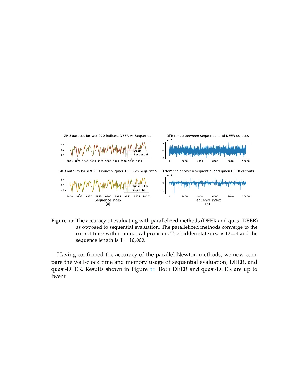
UNIFYING OPTIMIZA TION AND DYNAMICS T O P ARALLELIZE SEQUENTIAL COMPUT A TION: A GUIDE T O P ARALLEL NEWT ON METHODS FOR BREAKING SEQUENTIAL BOTTLENECKS A DISSER T A TION SUBMITTED TO THE DEP AR TMENT OF ST A TISTICS AND THE COMMITTEE ON GRADUA TE STUDIES OF ST ANFORD UNIVERSITY IN P ARTIAL FULFILLMENT OF THE REQUIREMENTS FOR THE DEGREE OF DOCTOR OF PHILOSOPHY Xa vier Gonzalez March 2026 Abstract Recurrent neural netw orks (RNNs) w ere widely regarded as "inherently sequen- tial" because each hidden state depends on the previous one. This sequential de- pendency creates a computational bottleneck: ev aluating an RNN on a sequence of length T seems to require O ( T ) time steps, ev en with unlimited parallel proces- sors. This dissertation challenges the conv entional wisdom and dev elops methods that enable parallel ev aluation of nonlinear RNNs with O (( log T ) 2 ) computational depth. Moreo v er , the methods I ha v e dev eloped and studied are v ery general, and can parallelize the broad class of computations falling under the heading of state space models (SSMs). SSMs include not only nonlinear RNNs but also Marko v chain Monte Carlo (MCMC), sampling from diffusion models, and explicit dif fer- ential equation solv ers, among many other applications. In my PhD, I built on an approach [ 41 , 142 ] that refor mulates RNN ev aluation as a ﬁxed-point problem and applies Newton’s method to lev erage the parallel scan algorithm. How ev er , when I began w ork on this subject, the community’s understanding of this parallel Newton method was hindered b y certain limitations. The Newton iterations suf fered from a lack of scalability in the state dimension D , a lack of stability in certain applications, and a general lack of understanding of its conv ergence properties and rates. In this thesis, I address these limitations with methodological and theoretical contributions. The methodological contributions of this thesis include dev eloping scalable and stable parallel Newton methods, based on quasi-Newton and trust-region approaches. The quasi-Newton methods further accelerate the training of RNNs and use a factor of D less memor y . The trust-region approaches are parallelized o v er the sequence length using a parallel Kalman ﬁlter and are signiﬁcantly more stable than their undamped counter parts. These methods ha v e inspired follo w-up w ork both in nonlinear sequence modeling and in parallelizing MCMC. The theoretical contributions of this thesis include establishing the conv ergence rates of parallel Ne wton methods. Both the Newton and quasi-Newton methods enjo y global conv ergence in at most T iterations. Moreo v er , w e show that the con- ditioning of the optimization landscape, as quantiﬁed by its Poly ak-Łojasiewicz (PL) constant, is determined by the stability of the dynamical system, as quanti- ﬁed by its Largest L y apunov Exponent (LLE). By doing so, w e show that stable (i.e. LLE < 0 ) dynamics enjoy conv ergence in O ( log T ) iterations, while unstable dynamics conv erge too slo wly for parallelization to w ork. In sum, this thesis unlocks scalable and stable methods for parallelizing sequen- tial computation, and pro vides a ﬁr m theoretical basis for when such techniques will and will not be ef fectiv e. This thesis also serv es as a guide to parallel Newton methods for researchers who want to write the next chapter in this ongoing stor y . iv Ackno wledgments Thank you to ev er y one who has made this PhD dissertation possible; and all who ha v e taught and mentored me ov er the years. Thank you to my advisor S cott Linderman for teaching me so much about research, collaboration, mentoring, softw are engineering, math, statistics, neuro- science, and more. Y ou hav e created one of the kindest and happiest labs at Stan- ford, and y ou are the driving force behind this social and collaborativ e culture. Speaking of the Linderman lab, thank y ou to all the amazing mentors and friends I’v e met in S cott’s lab. I am grateful for the opportunity to w ork with and learn from such talented researchers. Thank you to all my collaborators: I hav e lear ned so much and had so much fun w orking with y ou. Thank y ou in particular to the four postdocs who espe- cially mentored me on these projects: Andy W arrington, Leo Kozachkov , Kelly Buchanan, and David Zolto wski. Each of you taught me so much in different w a ys, and I am grateful for your gener osity of time and wisdom. Thank y ou to my family , friends, and mentors for their support and encourage- ment. Thank y ou especially to my parents Javier and Nataly a, my sister Natasha, and my girlfriend T iffany . Y our nurturing and support has made ev erything possible—and y our lov e has brightened my da ys. Ultimately , thank y ou to God—y ou are the source of all good things. Thank y ou for the many blessings of my PhD. v C O N T E N T S I i n t r o d u c t i o n a n d b a c k g r o u n d 1 1 i n t r o d u c t i o n 2 1 . 1 Extended History 3 1 . 2 Outline 6 2 b a c k g r o u n d 8 2 . 1 Dynamics: State Space Models 8 2 . 1 . 1 State Space Models (SSMs) 8 2 . 1 . 2 Examples of SSMs 9 2 . 1 . 3 Limitation of SSMs: "Inherently Sequential" 11 2 . 2 Parallel Computing: The Parallel Associativ e S can 12 2 . 2 . 1 The Parallel S can: A Gentle Introduction 12 2 . 2 . 2 Parallelizing Linear Dynamical Systems 14 2 . 2 . 3 Parallelizing Kalman Filtering and Smoothing 15 2 . 2 . 4 The Difﬁculties of Parallelizing an SSM in general 15 2 . 3 Numerical Analysis: Newton’s method 16 2 . 3 . 1 Root-ﬁnding 16 2 . 3 . 2 Optimization 20 2 . 3 . 3 Fixed-point methods 22 2 . 4 Putting it all together: Parallel Newton methods 23 2 . 4 . 1 Parallel Newton methods: DEER and DeepPCR 23 2 . 4 . 2 More in depth deriv ation 25 2 . 4 . 3 Limitations of Newton’s method 27 II m e t h o d s : s c a l a b l e a n d s t a b l e p a r a l l e l i z a t i o n 29 3 s c a l a b l e p a r a l l e l i z a t i o n : q u a s i - n e w t o n m e t h o d s 30 3 . 1 Quasi-DEER: A diagonal approximation 31 3 . 2 Global conv ergence 32 3 . 3 Experiments and performance of quasi-DEER 34 3 . 3 . 1 Quasi-DEER for Ev aluation 35 3 . 3 . 2 Quasi-DEER for T raining 36 3 . 4 Further dev elopment and directions for future w ork 38 3 . 4 . 1 Efﬁciently Estimating the Diagonal of the Jacobian 39 3 . 4 . 2 Generalizing quasi-DEER to other approximate Jacobians 40 3 . 4 . 3 T raining and the backwar ds pass 43 3 . 4 . 4 Initializing the guess for the state trajectory 45 4 s t a b l e p a r a l l e l i z a t i o n : e l k a n d t r u s t r e g i o n m e t h o d s 46 4 . 1 Lev enber g-Marquardt and T rust-Region Methods 46 vi 4 . 2 ELK: Ev aluating Lev enberg-Mar quardt with Kalman 48 4 . 3 Dynamics perspectiv e on ELK 50 4 . 4 Experiments and performance of ELK 52 4 . 4 . 1 Edge of stability: Parallelizing a sine w a v e 52 4 . 4 . 2 Chaotic system: Parallelizing the Lorenz 96 System 55 4 . 5 Further extensions: scale- and clip-ELK 57 4 . 5 . 1 S cale-ELK 58 4 . 5 . 2 Clip-ELK 58 4 . 6 Conclusion 58 III t h e o r y : c o n v e r g e n c e r a t e s 60 5 c o n v e r g e n c e r a t e s o f g au s s - n e w t o n f o r p a r a l l e l i z i n g n o n - l i n e a r s s m s 61 5 . 1 Predictability and the Largest L y apunov Exponent 61 5 . 2 Polyak-Łojasie wicz and Merit Landscape Conditioning 63 5 . 3 Conditioning depends on dynamical properties 65 5 . 3 . 1 Merit Function PL Constant is Controlled b y the Lar gest L y a- puno v Exponent of Dynamics 66 5 . 3 . 2 Residual function Jacobian Inherits the Lipschitzness of the Nonlinear State Space Model 67 5 . 4 Rates of Conv ergence for Optimizing the Merit Function 68 5 . 4 . 1 DEER Alw a ys Conv erges Globally at a Linear Rate 69 5 . 4 . 2 Size of DEER Basin of Quadratic Conv ergence 71 5 . 5 Experiments 74 5 . 5 . 1 The Conv ergence Rate Exhibits a Thr eshold betw een Pre- dictable and Chaotic Dynamics 74 5 . 5 . 2 DEER can conv erge quickly for predictable trajectories pass- ing through unpredictable regions 78 5 . 5 . 3 Application: Chaotic Observ ers 80 5 . 6 Discussion 81 5 . 6 . 1 Related W ork 82 5 . 6 . 2 Implications 82 5 . 7 Extensions 84 6 c o n v e r g e n c e r a t e s o f q ua s i - n e w t o n m e t h o d s f o r p a r a l - l e l i z i n g s s m s 86 6 . 1 Unifying ﬁxed-point iterations as quasi-DEER methods 87 6 . 1 . 1 Picard iterations 87 6 . 1 . 2 Jacobi iterations 89 6 . 1 . 3 Summary 89 6 . 2 Conv ergence rates for quasi-DEER 90 6 . 2 . 1 Conv ergence rates of ﬁxed-point iterations 91 6 . 2 . 2 Limitations of this conv ergence analysis 92 6 . 2 . 3 Intuitions about rates of conv ergence 93 vii 6 . 2 . 4 Summary of Conv ergence Analysis 97 6 . 3 Perfor mance of the different ﬁxed-point methods 98 6 . 3 . 1 Case study # 1 : Solving the group w ord problem with Ne w- ton iterations 98 6 . 3 . 2 Case Study # 2 : Picard iterations struggle to parallelize RNNs 100 6 . 3 . 3 Case Study # 3 : Jacobi iterations struggle to parallelize dis- cretized Langevin diffusion 103 6 . 4 Related W ork 104 6 . 5 Discussion 106 IV c o n c l u s i o n 108 7 c o n c l u s i o n a n d f u t u r e d i r e c t i o n s 109 7 . 1 Summar y of Contributions 109 7 . 2 Future Directions 110 7 . 2 . 1 Impro ving parallel Newton methods 110 7 . 2 . 2 Finding the best applications of parallel Newton methods 113 V a p p e n d i x 115 a g l o b a l c o n v e r g e n c e o f p a r a l l e l n e w t o n m e t h o d s 116 a . 1 Comparison of the tw o results 116 a . 2 Corrected v ersion of Theorem 3 . 6 of T ang et al. 118 b p r e d i c t a b i l i t y a n d c o n d i t i o n i n g 120 b . 1 Theorem statement and proof 120 b . 2 Discussion of why small singular v alues leads to ill-conditioning 122 b . 3 The dynamical inter pretation of the inv erse Jacobian 123 b . 3 . 1 Connection to semiseparable matrices and Mamba 2 124 b . 4 Framing based on global bounds 125 b . 5 Discussion of the LLE regularity conditions 125 b . 6 Controlling the maximum singular v alue 127 b . 7 Condition number of the Jacobian 128 c d i s c u s s i o n o f p a r a l l e l c h o r d m e t h o d s 129 b i b l i o g r a p h y 134 viii Part I I N T R O D U C T I O N A N D B A C K G R O U N D The ﬁrst part of this thesis pro vides the motiv ation and backgr ound for parallelizing dynamical systems. W e introduce the fundamental prob- lem of sequential computation in deep learning and review the mathe- matical foundations that enable parallel ev aluation of these models. haha gpus go brr Figure 1 : Parallel Newton methods. W ith a clev er connection betw een New- ton’s method and the parallel scan, w e can use GPUs to parallelize and therefore accelerate dynamical systems. 1 I N T R O D U C T I O N S equential processes are ubiquitous in statistics and machine lear ning. Ev aluat- ing a recurrent neural netw ork [ 81 ], sampling from a diffusion model [ 100 , 209 , 214 ] or with Marko v chain Monte Carlo (MCMC) [ 51 , 71 ], generating from a deep state space model [ 85 , 86 , 181 , 207 ], and unrolling la y ers of a deep neural net- w ork [ 96 , 226 ] all inv olv e sequential computations. Naiv ely , these computations require time proportional to the length of the input or the depth of the architec- ture, and in some cases, they ma y not take full adv antage of massiv ely parallel modern hardw are like graphics processing units (GPUs). For example, if the com- putational graph is a v ery long chain where each individual step in the chain is not too computationally intensiv e, but the chain is v ery long, this computational graph will not fully utilize the approximately 10 , 000 cores of a modern GPU. This mismatch betw een the requirements of sequential computation and the de- sign of moder n parallel hardw are has led to sequential models losing the "hard- w are lottery" [ 105 ] and being replaced by more easily parallelized architectures. This broad story is most clearly exempliﬁed in the transition from recurrent neu- ral netw orks (RNNs), the dominant sequence modeling architecture prior to 2018 , to war ds attention and the transfor mer architecture, an embarrassingly parallel approach that pow ers most of moder n AI, including the "generativ e pretrained transformers" behind ChatGPT and other moder n large language models (LLMs) [ 29 ]. In fact, as V asw ani et al. [ 226 ] write in the introduction to their landmark paper that introduced the transformer (emphasis added): Recurrent neural networks hav e been ﬁr mly established as state of the art approaches in sequence modeling and transduction problems such as language modeling and machine translation. How e v er , their inherently sequential nature precludes parallelization within train- ing examples , which becomes critical at longer sequence lengths, as memory constraints limit batching across examples. Despite signiﬁcant impro v ements in RNN computational efﬁciency , the fundamental con- straint of sequential computation remains. In the era of massiv ely parallel hardw are like GPUs, and e v er longer sequences of data to process, the "inherently sequential" [ 122 , 149 , 160 , 208 , 226 ] nature of RNNs w as view ed as a disqualifying disadv antage in many applications. 2 1 . 1 e x t e n d e d h i s t o r y 3 Incredibly , how e v er , as introduced in the seminal papers of Danieli et al. [ 41 ] and Lim et al. [ 142 ], nonlinear RNNs and many other types of "inherently se- quential" computations can be parallelized o v er the sequence length. This paral- lelization is achiev ed by recasting the problem of sequential ev aluation as a high- dimensional nonlinear equation that can be solv ed using Newton iterations that are parallelized ov er the sequence length. How ev er , when these parallel Newton methods w ere ﬁrst published, limitations blocked their wider use and adoption. These w ere standard limitations for Newton’s method in general [ 26 , 179 , 180 ], namely • A lack of scalability of the method, especially as the state size increased; • A lack of stability of the conv ergence of the method in certain applications; and • A lack of understanding of under what conditions the Newton iterations w ould converge , and at what rates. This dissertation helps to resolv e these limitations. Methodologically , w e intro- duce quasi-Newton methods to provide scalable parallelization and trust-region methods to pro vide stable parallelization. Theoretically , w e pro vide detailed con- v ergence analyses of these methods, including proofs of global conv ergence and the identiﬁcation of the stability of the underlying dynamical system as a critical decider of whether or not ef ﬁcient parallelization is possible. In doing so, w e ha v e unlocked scalable parallelization of nonlinear RNNs and a robust theoretical un- derstanding of under what conditions such parallelization is desirable. Moreo v er , these methods parallelize not only nonlinear RNNs [ 40 , 61 , 80 , 142 ] but can also parallelize a wide range of models called state space models (SSMs). In this thesis, an SSM is a discrete-time dynamical system with state s t ∈ R D that ev olv es o v er time by a transition function s t = f t ( s t − 1 ) (see S ection 2 . 1 ). Examples of chain-like computational graphs inv olving SSMs include sampling from MCMC [ 83 , 244 ] or diffusion models [ 41 , 90 , 153 , 199 , 201 , 221 ], solving differential equations with explicit methods [ 111 ], and many other div erse applications [ 78 ]. T aken together , this thesis la ys the foundation for exciting future w ork in paral- lelizing a br oad range of important primitiv es, while also more clearly delineating which processes are—and are not—"inherently sequential." This thesis ser v es as an introduction to parallel Newton methods for resear chers eager to contribute to this exciting, new ﬁeld. 1 . 1 e x t e n d e d h i s t o r y The moder n dev elopment of massiv ely parallel hardw are like GPUs and TPUs has created new urgency around the parallelization of sequential processes, con- tributing to the modern dev elopment of these parallel Newton methods [ 41 , 142 ]. 1 . 1 e x t e n d e d h i s t o r y 4 Ho w ev er , this thesis and the parallel Newton methods it sur v eys build on a long tradition of parallel-in-time computing [ 66 ]. In short, as long as there hav e been parallel computers and long sequences, there has been important w ork in paral- lelizing these sequential processes—and the modern massiv e increase in scale has led to a renaissance of these methods. While there w ere of course many earlier efforts at parallel computers, the IL- LIAC IV is widely credited as being the ﬁrst massiv ely parallel computer [ 15 ]. The ILLIAC IV w as dev eloped in the 1960 s and 1970 s at the Univ ersity of Illinois, and w as designed to hav e 256 processors that could carr y out computation in parallel. Almost immediately , this nov el dev elopment in hardw are led to nov el dev elop- ments in algorithms. For example, in 1973 , Stone [ 216 ] explicitly cited the ILLIAC as motiv ation for his dev elopment of a technique to solv e tridiagonal systems of equations 1 in parallel. Stone [ 216 ] called this method recursive doubling , and it is kno wn toda y as parallel cyclic reduction or the parallel associative scan . W e provide more background on the parallel scan as a general and fundamental primitiv e in S ection 2 . 2 . How e v er , to giv e a speciﬁc example, a canonical application of the parallel scan is as a technique to use T processors to multiply T matrices together in O ( log T ) computational depth—thus enabling exponential speedups on large parallel machines. In addition to the dev elopment of parallel methodology , the dev elopment of the ILLIAC also spurred fundamental w ork in the theor y of what computations could and could not be parallelized. For example, in 1975 , Hy aﬁl and Kung [ 110 ] and Kung [ 134 ] explicitly cited the ILLIAC as motiv ation for their study of which algorithms and models could be efﬁciently parallelized . They sho w ed that linear recursions enjoy speedups from parallel processors while nonlinear recursions of rational functions with degree larger than one in general cannot. These pre- scient w orks set the stage for the more general ﬁndings of this thesis presented in Part III , where w e explicitly link the dynamical properties of the recursion to its parallelizability . The desire to solv e differ ential equations o v er long time windows also led to the dev elopment of parallel-in-time methods for continuous-time initial value prob- lems (IVPs) [ 69 , 177 ]. While this dissertation primarily focuses on discrete-time SSMs, there are intimate links betw een discrete and continuous time, just as there are intimate links betw een dif ference and differential equations. In fact, the numer - ical solving of dif ferential equations almost alw a ys ev entually reduces to solving some discretization of the ordinary differential equation (ODE). Consequently , it is unsur prising that the ODE parallel-in-time, multiple shooting, and multigrid literature has many of the ingredients of moder n parallel Newton methods. For example, in 1989 Bellen and Zennaro [ 18 ] suggested a quasi-Newton method for 1 Which is extremely similar to parallel Newton methods, which in their simplest for m solv e bidiagonal systems of equations: see S ection 2 . 4 1 . 1 e x t e n d e d h i s t o r y 5 solving dif ferential equations that has almost all the core components of parallel Newton methods—except for the parallel scan. Indeed, the core ingredients of parallel Newton methods remained scattered throughout the parallel-in-time literature. For example, Horton, V andew alle, and W orley [ 106 ] proposed parallel-in-time solv ers for dif ferential equations using the parallel scan—but applied this technique to other ﬁxed-point iterations like Gauss- S eidel and Jacobi, not Newton. This pr eference for Gauss-S eidel and Jacobi iterations persisted in many strands of the literatur e. For example, Deshpande et al. [ 49 ] pro vided a theoretical analysis of conv ergence rates for these parallel-in-time methods. In discrete time, Naumo v [ 173 ] show ed how ev aluating Marko v chains could be cast as a system of nonlin- ear equations and discussed many techniques from numerical analysis for solving them, again focusing on Jacobi and Gauss-S eidel; S ong et al. [ 213 ] extended this program with many deep lear ning experiments. A possible explanation for this preference for Jacobi and Gauss-Seidel iterations is the hea vier computational cost of a single Newton iteration, especially on less massiv ely parallelized machines. On the other hand, when Newton iterations w ere suggested—as by Gander and V andew alle [ 67 ] as an interpretation of parareal iterations [ 145 ]—the link to par- allelization via the parallel scan w as omitted. Therefore, to the best of my knowledge, the full marriage betw een parallel scans and Newton iterations had to wait until 2023 and the seminal papers of Danieli et al. [ 41 ] and Lim et al. [ 142 ]—e v en though all the necessar y ingredients had ex- isted in the literature for at least thirty y ears. A likely factor in the dela y w as the fracturing of knowledge and motiv ations across different communities in dynam- ics, parallel computation, numerical analysis, and machine lear ning. Chapter 2 brings together the necessary background from all of these disciplines to close this gap and facilitate communication betw een these different communities. Undoubtedly the hardw are and software ecosystems also play ed a role in the ev entual dev elopment of parallel Ne wton’s method. In softw are, the standardiza- tion of autodiffer entiation [ 27 , 155 , 184 ] made the computation of Jacobians less burdensome. In hardw are, the dev elopment of GPUs with thousands of proces- sors and gigab ytes of on-device memor y made the cost of Newton iterations far less burdensome than they w ere on the ILLIAC and other earlier parallel ma- chines. The importance of these softw are and hardw are lotteries [ 105 ] in the de- v elopment of algorithms cannot be ov erstated. While this thesis pro vides an intro- duction to techniques that let us take "inher ently sequential" processes and reduce their latency on parallel hardw are, w e must remain open to the possibility that further de v elopments in hardw are, softw are, and algorithm ma y lead to y et more radically differ ent approaches in the future. 1 . 2 o u t l i n e 6 1 . 2 o u t l i n e In this introduction, w e pro vided a brief surv ey of the history of parallel compu- tation and parallel-in-time algorithms. In particular , w e discussed ho w the recent rise of massiv ely parallel processors like GPUs has further stimulated the advance- ment of parallel algorithms for "inherently sequential" computation. Building on this w ork, my thesis has dev eloped scalable methods for parallel-in-time com- putation and a ﬁrm theor etical understanding of under what conditions such parallel-in-time computation makes sense. The rest of this thesis is organized as follo ws: • Chapter 2 pro vides fundamental background for understanding parallel Newton methods, tying together dynamics, parallel computing, and numer - ical analysis. • Chapter 3 introduces our ﬁrst method, a quasi-Newton method for scalable parallelization. • Chapter 4 introduces our second method, a trust-region method for stable parallelization. • Chapter 5 establishes our theoretical analysis of conv ergence rates for the Gauss-Newton optimization method for parallelizing SSMs. • Chapter 6 studies the conv ergence rates of a wide class of quasi-Newton methods for parallelizing SSMs. • Chapter 7 concludes b y summarizing the contributions of this thesis and discussing promising directions for future w ork. The follo wing publications for m the basis of this dissertation: Chapters 3 and 4 are based on: Xavier Gonzalez , Andrew W arrington, Jimmy T .H. Smith, and S cott W . Linderman. "T o war ds S calable and Stable Parallelization of Nonlinear RNNs." In Advances in Neural Information Processing Systems (NeurIPS) , 2024 . Chapter 5 is based on: Xavier Gonzalez* , Leo Kozachkov*, David M. Zolto wski, Kenneth L. Clarkson, and S cott W . Linderman. "Predictability Enables Paralleliza- tion of Nonlinear State Space Models." In Advances in Neural Informa- tion Pr ocessing Systems (NeurIPS) , 2025 . 1 . 2 o u t l i n e 7 Chapter 6 is based on: Xavier Gonzalez* , E. Kelly Buchanan*, Hyun Dong Lee, Jerry W ei- hong Liu, Ke Alexander W ang, Da vid M. Zolto wski, Leo Kozachko v , Christopher Ré, and Scott W . Linder man. "A Unifying Framew ork for Parallelizing S equential Models with Linear Dynamical Systems." In T ransactions on Machine Learning Resear ch (TMLR) , 2026 . Throughout this thesis, w e also include material from Da vid M. Zolto wski*, Skyler W u*, Xavier Gonzalez , Leo Kozachkov , and S cott W . Linder man. "Parallelizing MCMC Across the S equence Length." In Advances in Neural Information Processing Systems (NeurIPS) , 2025 . This last paper extends and dev elops quasi-Newton methods to parallelize Markov chain Monte Carlo across the sequence length. 2 B A C K G R O U N D This thesis uses techniques from applied math to parallelize a class of sequen- tial processes known as state space models (SSMs) . Therefore, in this chapter , w e pro vide background on the three div erse foundational areas—dynamics, paral- lel computing, and optimization—so that w e can bring them together as parallel Newton methods . 2 . 1 d y n a m i c s : s t a t e s p a c e m o d e l s The ﬁrst topic this thesis brings into pla y is dynamics. In particular , w e study a class of sequential processes called state space models [ 172 ]. In this background section, w e deﬁne state space models, sur v ey their broad use in statistics and machine learning, and discuss why their e valuation w as deemed to be “inher ently sequential.” 2 . 1 . 1 State Space Models (SSMs) A state space model is a discrete-time dynamical system with a ﬁxed state size. W e denote this state b y s t ∈ R D , where the subscript t denotes the time of the state, and the dimension D denotes the state size. The state ev olv es according to a dynamics or transition function as s t + 1 = f t ( s t ) . ( 1 ) Importantly , state space models satisfy the Markov property , where the state at time t + 1 depends only on the state at time t , and not any of the previous states. Informally , the Marko v property means that once w e kno w the present, w e can forget the past. Our pr imar y consideration in this thesis is how to evaluate (equivalently “simulate”, “unroll” or “roll-out”) an SSM from an initial condition s 0 . W e make this goal precise in the follo wing problem statement: p r o b l e m s t a t e m e n t ( u n r o l l i n g a n s s m ) : Ev aluate the sequence s 1 : T = ( s 1 , s 2 , . . . , s T ) starting from s 0 , where s t follo ws the SSM dynamics in equation ( 1 ). Figure 2 indicates graphically ho w when w e unr oll the dynamics of an SSM from 8 2 . 1 d y n a m i c s : s t a t e s p a c e m o d e l s 9 s 0 s 1 s 2 s T − 1 s T f 1 f 2 f T · · · Figure 2 : Unrolling an SSM. W e shade the initial state s 0 to indicate that w e kno w the initial condition. s 0 s 1 s 2 s T − 1 s T u 1 u 2 u T − 1 u T f f f · · · ↕ s 0 s 1 s 2 s T − 1 s T f 1 f 2 f T · · · Figure 3 : Graphical diagram showing the equivalence (based on currying) between an SSM driv en b y inputs and an autonomous system with time-v ar ying transition dynamics. W e shade the inputs u t to indicate that they are kno wn. kno wn initial condition s 0 , w e obtain a computational graph that is a chain of sequential dependencies. Throughout this thesis, w e will use T to denote the se- quence length. Often, state space models also take an input u t ∈ R D at each time step. Thus, the dynamics become s t + 1 = f ( s t , u t ) . ( 2 ) Ho w ev er , as illustrated in Figure 3 , w e can alw a ys curry the input into the dynam- ics function to obtain an equivalent SSM without inputs. Speciﬁcally , w e deﬁne the curried dynamics functions as f t ( s t ) := f ( s t , u t ) . Thus, w e can rewrite the SSM with inputs as an SSM without inputs, as in equa- tion ( 1 ). While almost all the SSMs w e consider in this thesis take inputs, w e will often omit them from the notation for simplicity , relying on the fact that w e can alw a ys curr y them into the dynamics functions. 2 . 1 . 2 Examples of SSMs The framew ork giv en in equation ( 1 ) is extremely general, and many w ell-kno wn models in statistics and machine lear ning can be expressed as SSMs. W e summa- rize some important examples in T able 1 . 2 . 1 d y n a m i c s : s t a t e s p a c e m o d e l s 10 SSM State ( s t ) Input ( u t ) T ransition ( f ) Linear Dynamical Systems (LDS) [ 154 ] State Input Linear Deep SSMs [ 75 , 84 , 208 ] Stack of states Input Linear Recurrent Neural Netw orks (RNNs) [ 38 , 54 , 102 , 118 , 219 ] Hidden state Input RNN cell MCMC [ 51 , 71 , 244 ] Current sample Noise T ransition ker nel Sampling fr om diffusion models [ 137 , 201 , 210 ] Noisy image Noise Denoising func- tion Explicit differ - ential equation solv ers [ 66 , 111 , 125 ] Current state N/A Numerical inte- grator "Recurrent depth" for transfor mers [ 47 , 70 , 116 , 197 , 230 ] La y er activations Original input T ransfor mer block State of reinforce- ment learning (RL) agent [ 188 , 220 ] Environment state Noise Environment dy- namics Gradient descent [ 26 ] Parameter v alues N/A Gradient step The human brain [ 228 ] neural activity sensory input synapses T able 1 : Some illustrative examples of state space models (SSMs). The ﬁrst example in this T able 1 is the linear dynamical system (LDS) , which has linear transition dynamics, that is, the state ev olv es as s t + 1 = A t s t + B t u t . ( 3 ) Thus, an LDS is a special case of an SSM (equation ( 1 )), but where the dynamics function f t is afﬁne. These linear dynamical systems hav e enjo y ed a resurgence in machine lear ning recently as linear RNNs [ 160 , 181 ] or deep state space models 2 . 1 d y n a m i c s : s t a t e s p a c e m o d e l s 11 s 0 s 1 s 2 s 3 o 1 o 2 o 3 Figure 4 : A linear Gaussian state space model (LGSSM): The LGSSM consists of latent v ariables s t and obser v ed v ariables o t . The generativ e model of the LGSSM consists of dynamics s t + 1 ∼ N ( As t , Q ) and emissions o t + 1 ∼ N ( Cs t + 1 , R ) . [ 85 , 86 , 207 ]. In these deep lear ning architectures, the temporal dynamics of each la y er are linear , but the output of each lay er is passed through a nonlinearity to become the input of the next la y er . 2 . 1 . 2 . 1 Bayesian inference for linear Gaussian SSMs: Kalman ﬁltering and smoothing W e take a brief aside to discuss Ba y esian inference in state space models, as the core primitiv es of Kalman ﬁltering and smoothing are fundamental to our stable parallelization techniques dev eloped in Chapter 4 . W e begin b y noting that w e can include many probabilistic models into the SSM framew ork by incorporating stochastic inputs into our SSM dynamics equation equation ( 2 ). A fundamental probabilistic model is the linear Gaussian state space model (LGSSM), where the latent variables s t follo w linear dynamics with Gaus- sian noise, and emit observations o t with linear readouts with Gaussian noise [ 171 , 194 ]. S ee Figure 4 . In particular , note that the LGSSM is a simple w a y to make an LDS a probabilistic object: the latent variables s t are modeled as an LDS. T wo canonical inferential targets in the LGSSM are the ﬁltering distributions, p ( s t | o 1 : t ) , and the smoothing distributions, p ( s t | o 1 : T ) . The Kalman ﬁlter [ 119 ] and Rauch-T ung-Striebel (R TS) smoother 1 [ 189 ] obtain the ﬁltering and smoothing distributions (respectiv ely) in an LGSSM. The Kalman ﬁlter makes a single pass forwar d in time to get the ﬁltering distributions, while the R TS smoother then makes an additional pass backw ards in time to get the smoothing distributions. Thus, these canonical algorithms for Ba y esian inference in LGSSMs w ould also at ﬁrst glance seem to be inherently sequential. 2 . 1 . 3 Limitation of SSMs: "Inherently Sequential" Indeed, despite the breadth of use of SSMs across statistics and machine learn- ing, it w as widely believ ed that SSMs w ere “inherently sequential” to ev aluate [ 122 , 208 , 226 ]. W ith longer sequences, this sequential e valuation becomes a com- putational bottleneck, especially on modern hardw are like GPUs and TPUs that thriv e on parallelism. As a result, in keeping with the “hardw are lottery” [ 105 ], 1 Occasionally we will call the RTS smoother a “Kalman” smoother for simplicity . 2 . 2 p a r a l l e l c o m p u t i n g : t h e p a r a l l e l a s s o c i a t i v e s c a n 12 many researchers began to tur n a w a y from SSMs in fa v or of more parallelizable approaches. Ho w ev er , it tur ns out that there is a simple but ef fectiv e w a y to parallelize our ﬁrst and simplest example of SSMs in T able 1 : linear dynamical systems. Therefore, in our next background section on parallel computing, w e revie w the parallel as- sociative scan that allows us to parallelize linear dynamical systems. Ultimately , as w e will see in S ection 2 . 4 , a clev er use of the parallel scan allows us to parallelize SSMs in general , despite their “inherently sequential” nature. 2 . 2 p a r a l l e l c o m p u t i n g : t h e p a r a l l e l a s s o c i a t i v e s c a n The parallel scan [ 24 , 216 ], also kno wn as the associative scan and, colloquially , pscan , is a w ell-known primitiv e in the parallel computing literature [ 99 , 136 , 138 ]. The core idea of the parallel scan is a divide-and-conquer algorithm. W e illustrate this point in the simple example of multiplying a series of matrices together . 2 . 2 . 1 The Parallel Scan: A Gentle Intr oduction s i m p l e e x a m p l e : m u l t i p ly i n g a s e q u e n c e o f m a t r i c e s Consider the follo wing problem: giv en a series of square matrices A 1 , A 2 , . . . , A T − 1 , A T , compute their product 2 , A T A T − 1 . . . A 2 A 1 . The simplest w a y to carr y out the matrix mul- tiplication is sequentially: ﬁrst compute A 1 , then compute A 2 A 1 , then compute A 3 A 2 A 1 , and so on. Such an approach takes O ( T ) time. A core insight of the parallel scan is that matrix multiplication is closed ; that is, if A s ∈ R D × D and A t ∈ R D × D , then A t A s ∈ R D × D . Thus, matrix products can be computed recursiv ely in pairs, as illustrated in Figure 5 . A 1 A 2 A 3 A 4 A 2 A 1 A 4 A 3 A 4 A 3 A 2 A 1 Figure 5 : Parallel Scan for Matr ix Multiplication. W e illustrate a divide-and-conquer ap- proach to compute the product A 4 A 3 A 2 A 1 . Note that this divide-and-conquer approach naturally leads to O ( log T ) depth. Because of the divide-and-conquer (binar y-tree-like) nature of this approach to multiplying matrices, with O ( T ) processors, the time needed to get the matrix 2 Note that we ha v e the matrices act via left-multiplication o v er the sequence length, because this is the most common w a y to write matrix-v ector products. 2 . 2 p a r a l l e l c o m p u t i n g : t h e p a r a l l e l a s s o c i a t i v e s c a n 13 product is only O ( log T ) . This simple example illustrates the core intuition behind the parallel scan: a closed operation leading to a divide-and-conquer approach that parallelizes a computation so that it takes sublinear time. Ho w ev er , there are tw o additional details of the parallel associativ e scan that w e should address: arbi- trary binary associativ e operators and closure; and getting intermediate products. d e t a i l # 1 : p a r a l l e l s c a n s f o r a r b i t r a r y b i n a r y a s s o c i a t i v e o p e r a - t o r s Matrix multiplication is an associativ e operator , as A 3 ( A 2 A 1 ) = ( A 3 A 2 ) A 1 . In general, consider a binary associativ e operator ⊗ , which w ould satisfy q 3 ⊗ ( q 2 ⊗ q 1 ) = ( q 3 ⊗ q 2 ) ⊗ q 1 . No w , let us further assume that this binar y associativ e operator is closed: Deﬁnition 2 . 1 (Closure) . A binary associativ e operator ⊗ is closed ov er a set S if it satisﬁes the property: q 1 ∈ S , q 2 ∈ S ⇒ q 2 ⊗ q 1 ∈ S . ( 4 ) If ⊗ is closed, then w e can again use a parallel scan to compute the cumulativ e product of the operands. A wide range of binar y associativ e operators are closed, and can thus be par- allelized with the parallel scan. W e hav e already seen that matrix multiplication is such a binar y associativ e operator . An ev en simpler example of a binar y as- sociativ e operator amenable to the parallel scan is scalar addition . The fact that addition of scalars (and v ectors) is closed allows cumulativ e sums to be computed with the parallel scan algorithm. When the binar y associativ e operator is addition, it is also kno wn as the preﬁx sum algorithm. Clearly , addition is associativ e and closed, and so summing a series of scalars can be done with a divide-and-conquer approach. d e t a i l # 2 : o b t a i n i n g t h e i n t e r m e d i a t e t e r m s i n t h e p r o d u c t The parallel scan is meant to be a parallelized implementation of the S can primitiv e from functional programming [ 22 ]. Ho w ev er , S can not only returns the ﬁnal pr od- uct A T A T 1 . . . A 1 , as w e illustrated in Figure 5 , but also all the intermediate terms A 1 , A 2 A 1 , A 3 A 2 A 1 , etc. In fact, the parallel scan pro vides all the inter mediate ter ms as w ell. W e again illustrate in our motiv ating example of matrix multiplication, in particular the setting where T = 8 . W e will denote the individual matrices as A 1 , A 2 , A 3 , . . . A 8 , and their products as A s : t , i.e. A 5 : 6 = A 6 A 5 . The ﬁrst phase of the parallel scan is the up-sweep , and takes log ( T ) iterations and O ( T ) memor y . Crucially , note that w e are using O ( T ) processors in parallel as w ell. W e start multiplying adjacent pairs of matrices together . Looking, for example, at Position 8 of T able 2 , w e go from A 8 to A 7 : 8 to A 5 : 8 to A 1 : 8 . Then, in the down-sweep , w e ﬁll in the missing products to obtain all the cumu- lativ e products A 1 : t for 1 ⩽ t ⩽ T . Intuitiv ely , the do wn-sw eep also takes O ( log T ) 2 . 2 p a r a l l e l c o m p u t i n g : t h e p a r a l l e l a s s o c i a t i v e s c a n 14 iterations, for the same reason that any natural number T can be represented using 1 + log 2 ( T ) digits in binar y . Pos. 1 Pos. 2 Pos. 3 Pos. 4 Pos. 5 Pos. 6 Pos. 7 Pos. 8 A 1 A 2 A 3 A 4 A 5 A 6 A 7 A 8 A 1 A 1 : 2 A 3 A 3 : 4 A 5 A 5 : 6 A 7 A 7 : 8 A 1 A 1 : 2 A 3 A 1 : 4 A 5 A 5 : 6 A 7 A 5 : 8 A 1 A 1 : 2 A 3 A 1 : 4 A 5 A 5 : 6 A 7 A 1 : 8 T able 2 : Up-sw eep for multiplying A 1 , A 2 , . . . A 8 . Pos. 1 Pos. 2 Pos. 3 Pos. 4 Pos. 5 Pos. 6 Pos. 7 Pos. 8 A 1 A 1 : 2 A 3 A 1 : 4 A 5 A 1 : 6 A 7 A 1 : 8 A 1 A 1 : 2 A 1 : 3 A 1 : 4 A 1 : 5 A 1 : 6 A 1 : 7 A 1 : 8 T able 3 : Do wn-sweep for multiplying A 1 , A 2 , . . . A 8 . Thus, together , the up-sw eep and the do wn-sw eep of the parallel scan run in O ( log T ) time on O ( T ) processors, and at the end of this algorithm, w e get all of the intermediate products 3 (the “preﬁx sums”). 2 . 2 . 2 Parallelizing Linear Dynamical Systems Ha ving digested the fundamentals of the parallel scan, it becomes apparent that composition of af ﬁne functions is also a binary associativ e operator that is closed. Therefore, it is possible to parallelize ov er the sequence length the roll-out of an LDS ev olving according to equation ( 3 ). In more detail, consider the afﬁne function f i ( x ) = A i x + b i . Notice that the composition of afﬁne functions is also afﬁne, as f j ( f i ( x )) = A j A i x +  b j + A j b i  . Thus, if w e represent the operands as ordered pairs ( A i , b i ) and ( A j , b j ) , w e can write the associativ e operator ⊗ for the composition of afﬁne functions as ( A i , b i ) ⊗ ( A j , b j ) = ( A j A i , b j + A j b i ) . ( 5 ) Thus, w e obser v e that in this setting, ⊗ is closed. W e also should check that ⊗ is associativ e: w e can do so with either elementar y algebra, or b y obser ving that function composition is associativ e. This observation that composition of afﬁne functions can be parallelized with the associativ e scan is what lets us parallelize LDSs. The insight that LDSs could 3 See the last row of T able 3 . 2 . 2 p a r a l l e l c o m p u t i n g : t h e p a r a l l e l a s s o c i a t i v e s c a n 15 be parallelized with parallel scans led to a re v olution in the deep sequence mod- eling community based on transfor mer alter nativ e architectures. Because LDSs could be parallelized, this led to the dev elopment of both linear RNNs [ 160 , 181 ] and deep SSMs [ 85 , 207 ]. These approaches boil do wn to sequence mixing la yers that are LDSs (and ther efore parallelizable with parallel scan), stacked nonlin- early in depth. As w e will see throughout this thesis, decomposing nonlinear SSM dynamics into LDSs that can be parallelized with the parallel scan is our fundamental tool in parallelizing arbitrary SSMs. 2 . 2 . 3 Parallelizing Kalman Filtering and Smoothing In the pr evious section, w e sho w ed ho w w e can parallelize the ev aluation of a linear dynamical system. In this section, w e discuss ho w w e can also paral- lelize Ba y esian inference—Kalman ﬁltering and smoothing—in probabilistic mod- els based on LDSs, namely linear Gaussian SSMs (which w e re view ed in Subsec- tion 2 . 1 . 2 . 1 ). Both the Kalman ﬁlter and R TS smoother w ould seem to be inherently sequen- tial algorithms, requiring O ( T ) time. Ho w ev er , Särkkä and García-Fernández [ 192 ] demonstrated that the Kalman ﬁlter and R TS smoother can also be parallelized o v er the sequence length via the construction of custom binary associativ e opera- tors and a parallel scan. While w e lea v e the details of this construction to Särkkä and García-Fernández [ 192 ], w e note that it is intuitiv ely plausible to be able to parallelize ﬁltering and smoothing in an LGSSM with a parallel scan because • the dynamical backbone is an LDS, for which w e hav e a parallel scan (cf. equation ( 5 )); • since ev er ything is linear and Gaussian, all distributions remain Gaussian, hinting at closure; and • w e can combine p ( s t ′ | s 0 , o 1 : t ′ ) with p ( s t | s t ′ , o t ′ + 1 : t ) to obtain p ( s t | s 0 , o 1 : t ) , sug- gesting a divide-and-conquer strategy . These parallel ﬁltering and smoothing algorithms are useful in machine learning, allo wing for parallelization of structured variational autoencoders [ 115 , 243 ]. Sim- ilar approaches also w ork for Hidden Marko v Models [ 92 ] and for computing log-normalizing constants [ 107 ]. 2 . 2 . 4 The Difﬁculties of Parallelizing an SSM in general The astute reader might note that the composition of functions, i.e. f 1 ◦ f 2 , is al- ways a binar y associativ e operator . S o, why do w e hav e all these special cases of parallel scans, and not simply one parallel scan for the composition ◦ of arbitrar y functions f i ? 2 . 3 n u m e r i c a l a n a l y s i s : n e w t o n ’ s m e t h o d 16 The reason to ha v e many different parallel scans is precisely the importance of having the binary associativ e operator be closed . In all the previous examples, the binar y associativ e operator ⊗ satisﬁes Deﬁnition 2 . 1 , letting us easily store combinations of operands q i ⊗ q j and so emplo y a divide-and-conquer technique. While w e could consider some gigantic function space F , for which function composition would be closed, the practical question then becomes: ho w would w e store the combinations of operands? If w e do not ha v e some compact repre- sentation for elements of F , then w e cannot use a parallel scan in practice, ev en though the parallel scan ma y seem applicable in theor y . Nonetheless, w e still ha v e the parallel scan for parallelizing LDSs. When one has a hammer (the parallel scan for LDSs), ev er ything begins to look like a nail. Thus, one might attempt the seemingly hacky approach of taking nonlinear dy- namical systems, and iterativ ely • linearizing the system • ev aluating the linearized system in parallel with the parallel scan. Incredibly , this approach, which motiv ates this thesis, is not a hack but is rather an instantiation of Newton’s method! Therefore, in the next section, w e review Newton’s method in optimization and numerical analysis generally . 2 . 3 n u m e r i c a l a n a ly s i s : n e w t o n ’ s m e t h o d Newton’s method is one of the most fundamental approaches in r oot-ﬁnding, opti- mization, and numerical analysis generally [ 26 , 108 , 179 , 180 ]. In this background section, w e re view the fundamentals of Newton’s method and other related tech- niques in root-ﬁnding, optimization, and ﬁxed-point methods. 2 . 3 . 1 Root-ﬁnding Consider a high-dimensional nonlinear function r ( s ) : R P 7→ R P . A standar d prob- lem in numerical analysis is to ﬁnd the root of such a function, i.e. ﬁnd those s ⋆ for which r ( s ⋆ ) = 0 . In high dimensions and for a complicated function, it is not immediately ob vious how one might ﬁnd such a zero in an efﬁcient manner . Ho w ev er , if our function is afﬁne, i.e. r ( s ) = Ms + b , then provided M is inv ert- ible there is at least a straightforwar d wa y to ﬁnd the root s ⋆ , as s ⋆ = − M − 1 b . Newton’s method for root-ﬁnding for differentiable functions r is based on the idea of iterativ ely • linearizing r around our current guess s ( i ) to for m the afﬁne function ˆ r ( i ) ; and then • ﬁnding the root of ˆ r ( i ) , and making it our new guess s ( i + 1 ) . 2 . 3 n u m e r i c a l a n a l y s i s : n e w t o n ’ s m e t h o d 17 s r ( s ) 0 s ? s (0) s (1) s (2) s (3) Newton’s Metho d Figure 6 : Newton’ s method for root-ﬁnding. Here w e illustrate 3 iterations of New- ton’s method for root-ﬁnding on the one-dimensional cubic function r ( s ) = ( s − 0 . 4 ) 3 + 0 . 45 ( s − 0 . 4 ) . W e obser v e that each iteration of Newton’s method inv olv es linearizing the function to obtain ˆ r ( i ) ( · ) (sho wn in color) and then ﬁnd- ing the zer o of this linearization to obtain our next guess. W e sho w a graphical depiction of Newton’s method for a one-dimensional func- tion r ( · ) : R 7→ R in Figure 6 . Let us deﬁne the notational shorthand J ( i ) := ∂ r ∂ s ( s ( i ) ) , where w e choose J to stand for the Jacobian matrix (i.e. deriv ativ e) of r . W ith this notation, w e see that the ﬁrst step is giv en b y a ﬁrst-order T a ylor expansion of r around s ( i ) , i.e. ˆ r ( i ) ( s ) := r ( s ( i ) ) + J ( i )  s − s ( i )  . Thus, w e see that ev er y step of Ne wton’s method for root-ﬁnding—where w e aim to ﬁnd the zero of ˆ r ( i ) ( s ) —is giv en b y s ( i + 1 ) = s ( i ) −  J ( i )  − 1 r ( s ( i ) ) . ( 6 ) Of course, for equation ( 6 ) to be valid, w e must ha v e J ( i ) inv ertible—but for the parallel Newton methods considered in this dissertation, it alw a ys will be (see equation ( 17 )). Another limitation of Newton’s method immediately visible from equation ( 6 ) is the need to store and inv ert J ( i ) ∈ R P × P . In particular , the matrix inv ersion requires O ( P 3 ) ﬂoating point operations (FLOPs). While the implementation of the numerical linear algebra can be optimized [ 77 ], the ov erall cost of Newton’s method has inspir ed a br oad literature on cheaper , approximate quasi-Newton 2 . 3 n u m e r i c a l a n a l y s i s : n e w t o n ’ s m e t h o d 18 methods [ 148 , 178 , 179 ]. W e build on and contribute to this quasi-Ne wton lit- erature in Chapter 3 . While Figure 6 sho ws intuitiv ely why Newton’s method can be a po w erful tech- nique for root-ﬁnding, let us discuss some of its conv ergence properties further and more formally . c o n v e r g e n c e o f n e w t o n ’ s m e t h o d Newton’s method is kno wn to enjo y quadratic conver gence within a basin around the solution s ⋆ [ 108 , 179 , 180 ]. One w a y to deﬁne quadratic conv ergence, following the presentation in No- cedal and W right [ 179 ], is via the notion of Q-convergence , which is short for quotient-convergence : Deﬁnition 2 . 2 (Q-conv ergence) . Consider a sequence of iterates { s ( i ) } which is conv erging to a limit s ⋆ as i → ∞ . Then this sequence Q-conv erges to s ⋆ with order q and with rate of convergence γ if, for all ( i ) suf ﬁciently large, ∥ e ( i + 1 ) ∥ ⩽ γ ∥ e ( i ) ∥ q , ( 7 ) where the err ors are deﬁned b y e ( i ) := s ( i ) − s ⋆ , ( 8 ) and ∥ · ∥ is any v alid v ector norm. If the order q = 1 , w e say that the iterativ e method enjoys linear convergence , while if q = 2 , it enjo ys quadratic convergence . In linear conv ergence, the err or sat- isﬁes 4 ∥ e ( i ) ∥ ⩽ γ i ∥ e ( 0 ) ∥ , indicating that the nor m of the error deca ys exponen- tially in the number of iterations, with base γ . W e must hav e γ < 1 for linear conv ergence to conv erge to a limit. In quadratic conv ergence, the error satisﬁes ∥ e ( i ) ∥ ⩽ ( γ ∥ e 0 ∥ ) 2 i / γ , indicating the norm of the error deca ys doubly-exponentially with base γ ∥ e 0 ∥ . Again, ho w ev er , to actually enjoy decrease with quadratic conv er- gence, w e must ha v e γ ∥ e 0 ∥ < 1 , giving rise to the basin of quadratic conver gence B Q giv en b y B Q :=  s ( i ) : ∥ s ( i ) − s ⋆ ∥ < 1 γ  . W ith this deﬁnition, w e no w pro vide a simple proof 5 that Newton’s method enjo ys quadratic rate in a basin around the solution s ⋆ . Proposition 2 . 3 . Say we are trying to ﬁnd a root of r ( s ) : R P 7→ R P with Newton’ s method as deﬁned in equation ( 6 ) . If we assume that J ( s ) is L -Lipschitz and is always invertible with ∥ J ( s ) − 1 ∥ ⩽ β for all s , then Newton’ s method converges quadratically in the basin given by  s ( i ) : ∥ s ( i ) − s ⋆ ∥ ⩽ 2 Lβ  . 4 Here, w e slightly abuse notation to make e ( 0 ) the ﬁrst iteration where the inequality in ( 7 ) holds. 5 follo wing e.g. the proof of Proposition 4 of Lu, Zhu, and Hou [ 153 ]. 2 . 3 n u m e r i c a l a n a l y s i s : n e w t o n ’ s m e t h o d 19 Proof. Subtract s ⋆ from both sides of equation ( 6 ) to obtain e ( i + 1 ) = e ( i ) −  J ( s ( i ) )  − 1 r ( s ( i ) ) . T aylor expanding r ( · ) around s ( i ) , w e get the equality r ( s ⋆ ) = r ( s ( i ) ) − J ( s ( i ) ) e ( i ) + R ( i ) , where the remainder R ( i ) satisﬁes ∥ R ∥ ⩽ L 2 ∥ e ( i ) ∥ 2 . Since r ( s ⋆ ) = 0 , it follo ws that e ( i + 1 ) =  J ( s ( i ) )  − 1 R ( i ) . T aking nor ms on both sides and inputting the assumptions, it follows that ∥ e ( i + 1 ) ∥ ⩽ Lβ 2 ∥ e ( i ) ∥ 2 , i.e. Newton’s method enjo ys quadratic conv ergence in the speciﬁed basin. Ho w ev er , this quadratic conv ergence of Newton’s method only holds locally , i.e. for initial guesses s ( 0 ) that are close to the zero s ⋆ . It is stronger and more helpful to ha v e guarantees for global conv ergence, i.e. assurances that an iterativ e solv er will conv erge (and with a speciﬁed rate) no matter the initial guess s ( 0 ) . Unfortunately , in general, Ne wton’s method does not enjoy global conv ergence guarantees [ 179 ]. W e illustrate with a simple example. s r ( s ) = s 1 / 3 0 s (0) s (1) s (2) s (3) Newton’s Metho d Divergence (Cub e Ro ot) Figure 7 : Newton’ s method can globally diverge. A graphical depiction showing how Newton’s method for root-ﬁnding can globally diverge for a simple function like r ( s ) = s 1/3 . 2 . 3 n u m e r i c a l a n a l y s i s : n e w t o n ’ s m e t h o d 20 Example 2 . 4 (Newton’s method can div erge: r ( s ) = s 1/3 .) . Consider the standard cube root function r ( s ) = s 1/3 deﬁned on all of the real line. At all points s ∈ R , the derivative of this function is given by r ′ ( s ) = 1 3 s − 2/3 . So, plugging into equation ( 6 ) , it follows that, no matter the initial guess, the Newton iterates follow s ( i + 1 ) = − 2 s ( i ) . Consequently , we observe that for any initial guess not the unique solution s ⋆ = 0 , New- ton’ s method will diver ge for this function, as shown in Figure 7 . Note that Pr oposition 2 . 3 does not even apply in this setting because the derivative is neither Lipschitz nor does its inverse have a uniform bound. Studying the conv ergence rates of parallel Newton methods—as w ell as their possible instabilities—is a major theme of this thesis. 2 . 3 . 2 Optimization While Ne wton’s method is usually ﬁrst presented in an introduction to calculus as a method for root-ﬁnding (Subsection 2 . 3 . 1 ), it is best known in machine learning in the context of optimization. Say w e ha v e an objectiv e function F ( s ) : R P → R that is twice differ entiable, and w e wish to ﬁnd its minimum, i.e. s ⋆ = argmin s ∈ R P F ( s ) . For large dimension P and a complicated objectiv e function F ( s ) , optimization can be v ery difﬁcult. In fact, the problem of high-dimensional optimization is one of the central problems of machine learning [ 89 , 117 , 127 , 227 ]. Ho w ev er , if F ( s ) is a conv ex quadratic function, i.e. w e can write F ( s ) = 1 2 s ⊤ Ms + b ⊤ s + c for positiv e-deﬁnite matrix M , then its unique minimizer is giv en b y s ⋆ = − M − 1 b . Thus, Newton’s method for optimization of a twice-differentiable function is directly analogous to Newton’s method for r oot-ﬁnding for a differentiable func- tion. In Ne wton’s method for root-ﬁnding, w e built on the fact that w e could solv e inv ertible linear systems, and so for a nonlinear system r ( s ) = 0 , w e iterativ ely lin- earize r ( · ) and solv e. In Newton’s method for optimization, w e build on the fact that w e ha v e a closed form solution for the minimum of a conv ex quadratic, and so for a twice-differentiable function F ( · ) , w e iterativ ely build and minimize the quadratic surrogate of F ( · ) . The quadratic surrogate for F ( · ) at our current guess s ( i ) is giv en b y ˆ F i ( s ) = F ( s ( i ) ) + ∇ s F ( s ( i ) ) ⊤  s − s ( i )  + 1 2  s − s ( i )  ⊤ ∇ 2 s F ( s ( i ) )  s − s ( i )  , ( 9 ) 2 . 3 n u m e r i c a l a n a l y s i s : n e w t o n ’ s m e t h o d 21 where ∇ 2 s F ( s ( i ) ) ∈ R P × P is the Hessian of F ( · ) ev aluated at s ( i ) . Therefore, if the Hessian is positiv e-deﬁnite, the minimizer of ˆ F i ( s ) , and therefore the formula for the next iteration in Newton’s method for optimization, is s ( i + 1 ) := −( ∇ 2 s F ( s ( i ) )) − 1  ∇ s F ( s ( i ) ) − ∇ 2 s F ( s ( i ) ) s ( i )  = s ( i ) − ( ∇ 2 s F ( s ( i ) )) − 1 ∇ s F ( s ( i ) ) . Ho w ev er , w e recognize this update for Newton’s method for optimization as the same as Newton’s method for root-ﬁnding in equation ( 6 ), where the function w e are ﬁnding the root of is ∇ s F ( · ) : R P → R P . Thus, w e see that Newton’s method for optimization of a function F ( · ) is nothing more than Newton’s method for r oot- ﬁnding applied to the derivative of F ( · ) . This connection is part of the rich inter pla y in numerical analysis betw een root- ﬁnding (ﬁnding the zero of a function) and optimization (ﬁnding the minima of a function) [ 179 ]. The fact that Newton’s method for optimization of objectiv e function F ( · ) is equiv alent to Newton’s method for root-ﬁnding applied to its deriv ativ e ∇ F ( · ) makes sense because for a differentiable function F ( s ) : R P → R , its minima lie among its stationary points (the set of points where its derivativ e ∇ F ( s ) = 0 ). g a u s s - n e w t o n m e t h o d f o r o p t i m i z a t i o n o f s u m - o f - s q ua r e s How- ev er , there are ev en more connections betw een root-ﬁnding and optimization. If w e return to the problem of ﬁnding a root of a residual function r ( s ) : R P → R P , w e obser v e that w e can for m a merit function L ( s ) := 1 2 ∥ r ( s ) ∥ 2 2 . ( 10 ) Because L ( s ) is a sum-of-squares objectiv e, it is greater than or equal to zero, and w e obser v e that L ( s ⋆ ) = 0 , meaning the root s ⋆ of r ( · ) is also the minimizer of the merit function 6 L ( · ) . By basic calculus, w e obser v e that the gradient and Hessian of L are giv en b y ∇ L ( s ) = J ⊤ r ∇ 2 L ( s ) = J ⊤ J + P X i = 1 r i ( s ) ∇ 2 r i ( s ) , where J ( s ) := ∂ r ∂ s ( s ) . 6 While it is admittedly counterintuitiv e to desire to "minimize" a "merit function," w e follow the naming conv ention set b y the classic textbook Nocedal and W right [ 179 ]. 2 . 3 n u m e r i c a l a n a l y s i s : n e w t o n ’ s m e t h o d 22 While w e could apply Newton’s method for optimization to L , w e kno w from our previous discussion that this w ould be Ne wton’s method for root-ﬁnding applied to the gradient ∇ L ( s ) = J ⊤ ( s ) r ( s ) , and not Newton’s method for root- ﬁnding applied to the original residual function r ( s ) . Ho w ev er , a v er y simple modiﬁcation called the Gauss-Newton method restores the link betw een optimization of the sum-of-squares merit function L and root- ﬁnding of the residual r . In the Gauss-Newton method, w e apply Newton’s method, but w e approximate the Hessian b y J ⊤ J . The Gauss-Ne wton method is thus a w a y to get the beneﬁt of second-order methods while only taking one deriv ativ e. More- o v er , its updates take the for m s ( i + 1 ) = s ( i ) −  J ⊤ J  − 1 J ⊤ r . If J is inv ertible, then the Gauss-Newton updates take the form s ( i + 1 ) = s ( i ) − J − 1 r , which w e again recognize as equation ( 6 ), i.e. root-ﬁnding for r . Note, therefore, that if J is inv ertible, then Gauss-Newton as an optimization technique for L is mathematically equiv alent to Newton’s method for r oot ﬁnding applied to r . For this reason, another interpretation of the Gauss-Ne wton method is as linearizing the residual function r ( s ) : that is, each step of the Gauss-Newton method minimizes the quadratic loss ˆ L s ( i ) ( s ) := 1 2    r ( s ( i ) ) + J ( s ( i ) )  s − s ( i )     2 2 . For small residuals, the Ne wton and Gauss-Newton methods ha v e similar con- v ergence properties (cf. [ 179 ]). Importantly , just like Newton’s method for root- ﬁnding, they can also both div erge globally . For example, take Example 2 . 4 and turn it into an optimization problem with objectiv e function F ( s ) = s 4/3 to see that Newton’s method will div erge or merit function L ( s ) = s 2/3 to see that Gauss- Newton will div erge. 2 . 3 . 3 Fixed-point methods W e can also write each step of Newton’s method as the action of an operator A N ( s ) : R P → R P , i.e. s ( i + 1 ) = A N ( s ( i ) ) A N ( s ( i ) ) = s ( i ) −  J ( i )  − 1 r ( s ( i ) ) . 2 . 4 p u t t i n g i t a l l t o g e t h e r : p a r a l l e l n e w t o n m e t h o d s 23 Importantly note that if s ⋆ is a root of r ( s ) , i.e. r ( s ⋆ ) = 0 , then it follo ws that A N ( s ⋆ ) = s ⋆ , i.e. s ⋆ is a ﬁxed-point of the Newton’s method operator A N . In general, a ﬁxed-point problem aims to ﬁnd s ⋆ satisfying F ( s ⋆ ) = s ⋆ , for some function F ( s ) : R P → R P . Any ﬁxed-point problem can be inter preted as a root-ﬁnding problem b y deﬁning r ( s ) = s − F ( s ) , and then asking to ﬁnd s ⋆ such that r ( s ⋆ ) = 0 . Because of all of these connections, Newton’s method is also a foundational concept in ﬁxed-point methods and solv ers [ 180 ]. As w e will see in Chapter 6 , many differ ent ﬁxed-point methods can be used to parallelize SSMs, including Picard and Jacobi iterations. W e discuss in more detail in that section. 2 . 4 p u t t i n g i t a l l t o g e t h e r : p a r a l l e l n e w t o n m e t h o d s In the pr evious sections, w e re view ed dynamics, parallel computation, and numer - ical analysis, with the goal of combining these three div erse ﬁelds to parallelize the unrolling of state space models. In this section, w e combine these three ingre- dients to show ho w parallel Newton methods allow for the parallelization of such “inherently sequential” processes. 2 . 4 . 1 Parallel Newton methods: DEER and DeepPCR Concurrently , Lim et al. [ 142 ] dev eloped DEER and Danieli et al. [ 41 ] dev eloped DeepPCR, both of which are the same parallel Newton method for the paralleliza- tion of SSMs. This section re views their foundational w ork. Throughout this the- sis, w e use the ter ms “DeepPCR”, “DEER”, and “parallel Newton methods” inter - changeably . The fundamental idea of parallelizing SSMs is to replace sequential e v aluation with parallel iterative ev aluation. W e compare these tw o approaches to ev aluating an SSM in Figure 8 . Going for w ard, w e will denote the true roll-out from the SSM ov er the entire trajector y of length T as s ⋆ ∈ R T D , i.e. s ⋆ 1 = f 1 ( s 0 ) , s ⋆ 2 = f 2 ( s ⋆ 1 ) , and in general s ⋆ t = f t ( s ⋆ t − 1 ) . 7 Note that at initialization, s ⋆  = s ( 0 ) , i.e. w e ma y be initializing in a wa y that is not faithful at all to the true SSM dynamics. Thus, w e 7 In our discussion of parallel Newton methods, and henceforth in this thesis, w e will use bold script for v ariables of shape T D or T D × T D , and not bold for v ariables of shape D or D × D . So, bolding will be reser v ed for variables that extend ov er the sequence length, while variables that are just at a particular point in time will not be bolded. W e follow this conv ention to distinguish between operations that occur across the sequence length vs. at a particular point. 2 . 4 p u t t i n g i t a l l t o g e t h e r : p a r a l l e l n e w t o n m e t h o d s 24 . S equent ia l v s P a ra llel Ev a lua t io n T o w a r d s S c a l a b l e a n d S t a b l e Pa r a l l e l i z a t i o n o f N o n l i n e a r R N N s Xa v ie r Go nza le z, A ndre w Wa rringt o n, Jim m y T .H. S m it h, S co t t W. Linde rm a n {xavier18, scott.linderman }@ stanford.edu 1. X. G o n z a l e z , A . W a r r i n g t o n , J . S m i t h , a n d S . L i n d e r m a n . T o w a r d s S c a l a b l e a n d S t a b l e Pa r a l l e l i za t i o n o f N o nl i ne a r R N N s . Ad v a n c e s i n N e u r a l I n f or m a t i on Pr oc e s s i n g S y s t e m s , 2024 . 2. YH L i m , Q . Z h u , J . S e l f r i d g e , a n d M . K a s i m . P a r a l l e l i z i n g n o n - lin e a r s e q u e n t ia l m o d e ls o v e r th e s e q u e n c e l e n g th . In t e r n a t i o n a l C o n f e r e n c e o n L e a r n i n g R e p r e s e n t a t i o n s , 2024 . 3. S. Sa r k k a an d A . G ar c i a - Fe r n a n d e z . T e m p o r a l p a r a l l e l i z a t i o n o f B a y e s i a n s m o o t h e r s . IE E E Tr a n s a c t i o n s o n A u t o m a t i c C o n t r o l . 2 0 2 1 . 4. S. Sa r k k a an d L. Sv e n s s o n . L e v e n b e r g - Ma r q u a r d t a n d l i n e - se a r c h e x t e n d e d K a l m a n sm o t h e r s. IC A S S P 2 0 2 0 - 20 20 I E E E I n t e rn a t i o n a l C o n f e re n c e o n A c o u st i c s, S p e e c h a n d S i g n a l Pr o c e s s i n g ( I C AS S P) . 2 0 2 0 . Referen c es Pap e r L i n k - Pa r a l l el i z ed sequ en c e m o del l i n g i s im p o rt an t . Co ns i d e r Tr a ns f o r m e r s a nd d e e p S S M s ( l i ne a r R N N s ) . - Non lin e ar R NNs c an als o b e p aralle liz e d b y t re at in g t h e m a s t h e s o l u t i o n o f f i x e d p o i n t e q u a t i o n ( D EER 2 , Li m et a l , ‘ 2 4 ) - Pa r a l l el i z i n g n o n l i n ea r R N N s c a n a c c el er a t e t h ei r e v a l u a t i o n a n d t r a i n i n g b y m a k i n g b e t t e r u s e o f GP U s - We m a k e p a r a l l e l i z i n g RN N S sc a l a bl e us i ng a q ua s i - Ne w t on m e t h od an d st a bl e us i ng a tr us t - re g io n S um m a ry - The r e s i d ua l ( w ha t w e w a nt t o f i nd t he r o o t o f ) i s - So , t h e J a c o bi a n in t h is part ic u lar pro ble m is - De f in e t h e Ne w t on s t e p as - The N e w t o n s t e p i s t he s o l ut i o n o f a s o l v e , i .e . f i nd sa t i sf y i n g - Bec a u se h a s bl o c k bi di a go n a l st r u c t u r e, t h i s so l v e c a n be ev a l u a t ed u si n g f o r wa r d su bst i t u t i o n . - The f o r w a r d s ub s t i t ut i o n g i v e s a s i m p l e l i ne a r r e c ur s i o n wi t h t h e i n i t i a l c o n di t i o n , a n d f o r t> 1 B a c k gro und: D EER & N ew t o n’ s m et ho d . A lgo rit hm s . P a ra llel S c a n - Ma k e di a go n a l a ppr o x i m a t i o n . - Qua s i - Ne w t on u p d at e . - Co m p ute & m e m o r y e f f i c i e nt. S t a bilit y : EL K - Ne w t on ’ s m e t h od c an b e s t ab iliz e d w it h a t ru s t re g ion . - The r e s ul t i ng p e na l i ze d o b j e c t i v e i s t he s o l ut i o n t o a Ka l m a n s m o o the r 3 an d c an b e p aralle liz e d 4 . Fig ure 2: Sequent ial evalua tion ve rsus parallel it erative ev aluation . Left: Se q u e n t ia l e v a lu a t io n s t e p s t h ro u g h t h e s e q u e n c e . Ri gh t : Pa ra lle l e v a lu a t io n i t e r a t e s o v e r t h e w h o l e s e q u e n c e , a n d c a n c o n v e r g e i n fe w e r s t e p s . 12 Presentation s 0 s 1 s 2 s 3 s 4 s ( 0 ) 1 s ( 0 ) 2 s ( 0 ) 3 s ( 0 ) 4 s ( 1 ) 1 s ( 1 ) 2 s ( 1 ) 3 s ( 1 ) 4 + ∆ s ( 1 ) + ∆ s ( 2 ) + ∆ s ( i ) J t > 1 r ( s 1: T ) : =[ s 1 − f ( s 0 ) , s 2 − f ( s 1 ) ,. .. , s T − f ( s T − 1 )] J ( s ) : = ∂ r ∂ s ( s )= ⎛ ⎜ ⎜ ⎜ ⎜ ⎜ ⎝ I D 0. . . 0 0 − ∂ f ∂ s ( s 1 ) I D .. . 0 0 . . . . . . . . . . . . . . . 00 . . . I D 0 00 . . . − ∂ f ∂ s ( s T − 1 ) I D ⎞ ⎟ ⎟ ⎟ ⎟ ⎟ ⎠ . ∆ s ( i + 1 ) : = s ( i + 1 ) − s ( i ) ∆ s 40 12 Presentation s 0 s 1 s 2 s 3 s 4 s ( 0 ) 1 s ( 0 ) 2 s ( 0 ) 3 s ( 0 ) 4 s ( 1 ) 1 s ( 1 ) 2 s ( 1 ) 3 s ( 1 ) 4 + ∆ s ( 1 ) + ∆ s ( 2 ) + ∆ s ( i ) J t > 1 r ( s 1: T ) : =[ s 1 − f ( s 0 ) , s 2 − f ( s 1 ) ,. .. , s T − f ( s T − 1 )] J ( s ) : = ∂ r ∂ s ( s )= ⎛ ⎜ ⎜ ⎜ ⎜ ⎜ ⎝ I D 0. . . 0 0 − ∂ f ∂ s ( s 1 ) I D .. . 0 0 . . . . . . . . . . . . . . . 00 . . . I D 0 00 . . . − ∂ f ∂ s ( s T − 1 ) I D ⎞ ⎟ ⎟ ⎟ ⎟ ⎟ ⎠ . ∆ s ( i + 1 ) : = s ( i + 1 ) − s ( i ) ∆ s 40 12 Presentation s 0 s 1 s 2 s 3 s 4 s ( 0 ) 1 s ( 0 ) 2 s ( 0 ) 3 s ( 0 ) 4 s ( 1 ) 1 s ( 1 ) 2 s ( 1 ) 3 s ( 1 ) 4 + ∆ s ( 1 ) + ∆ s ( 2 ) + ∆ s ( i ) J t > 1 r ( s 1: T ) : =[ s 1 − f ( s 0 ) , s 2 − f ( s 1 ) ,. .. , s T − f ( s T − 1 )] J ( s ) : = ∂ r ∂ s ( s )= ⎛ ⎜ ⎜ ⎜ ⎜ ⎜ ⎝ I D 0. . . 0 0 − ∂ f ∂ s ( s 1 ) I D .. . 0 0 . . . . . . . . . . . . . . . 00 . . . I D 0 00 . . . − ∂ f ∂ s ( s T − 1 ) I D ⎞ ⎟ ⎟ ⎟ ⎟ ⎟ ⎠ . ∆ s ( i + 1 ) : = s ( i + 1 ) − s ( i ) ∆ s 40 12 Presentation s 0 s 1 s 2 s 3 s 4 s ( 0 ) 1 s ( 0 ) 2 s ( 0 ) 3 s ( 0 ) 4 s ( 1 ) 1 s ( 1 ) 2 s ( 1 ) 3 s ( 1 ) 4 + ∆ s ( 1 ) + ∆ s ( 2 ) + ∆ s ( i ) J t > 1 r ( s 1: T ) : =[ s 1 − f ( s 0 ) , s 2 − f ( s 1 ) ,. .. , s T − f ( s T − 1 )] J ( s ) : = ∂ r ∂ s ( s )= ⎛ ⎜ ⎜ ⎜ ⎜ ⎜ ⎝ I D 0. . . 0 0 − ∂ f ∂ s ( s 1 ) I D .. . 0 0 . . . . . . . . . . . . . . . 00 . . . I D 0 00 . . . − ∂ f ∂ s ( s T − 1 ) I D ⎞ ⎟ ⎟ ⎟ ⎟ ⎟ ⎠ . ∆ s ( i + 1 ) : = s ( i + 1 ) − s ( i ) ∆ s 40 12 Presentation s 0 s 1 s 2 s 3 s 4 s ( 0 ) 1 s ( 0 ) 2 s ( 0 ) 3 s ( 0 ) 4 s ( 1 ) 1 s ( 1 ) 2 s ( 1 ) 3 s ( 1 ) 4 + ∆ s ( 1 ) + ∆ s ( 2 ) + ∆ s ( i ) J t > 1 r ( s 1: T ) : =[ s 1 − f ( s 0 ) , s 2 − f ( s 1 ) ,. .. , s T − f ( s T − 1 )] J ( s ) : = ∂ r ∂ s ( s )= ⎛ ⎜ ⎜ ⎜ ⎜ ⎜ ⎝ I D 0. . . 0 0 − ∂ f ∂ s ( s 1 ) I D .. . 0 0 . . . . . . . . . . . . . . . 00 . . . I D 0 00 . . . − ∂ f ∂ s ( s T − 1 ) I D ⎞ ⎟ ⎟ ⎟ ⎟ ⎟ ⎠ . ∆ s ( i + 1 ) : = s ( i + 1 ) − s ( i ) ∆ s 40 12 Presentation s 0 s 1 s 2 s 3 s 4 s ( 0 ) 1 s ( 0 ) 2 s ( 0 ) 3 s ( 0 ) 4 s ( 1 ) 1 s ( 1 ) 2 s ( 1 ) 3 s ( 1 ) 4 + ∆ s ( 1 ) + ∆ s ( 2 ) + ∆ s ( i ) J t > 1 r ( s 1: T ) : =[ s 1 − f ( s 0 ) , s 2 − f ( s 1 ) ,. .. , s T − f ( s T − 1 )] J ( s ) : = ∂ r ∂ s ( s )= ⎛ ⎜ ⎜ ⎜ ⎜ ⎜ ⎝ I D 0. . . 0 0 − ∂ f ∂ s ( s 1 ) I D .. . 0 0 . . . . . . . . . . . . . . . 00 . . . I D 0 00 . . . − ∂ f ∂ s ( s T − 1 ) I D ⎞ ⎟ ⎟ ⎟ ⎟ ⎟ ⎠ . ∆ s ( i + 1 ) : = s ( i + 1 ) − s ( i ) ∆ s 40 12 Presentation s 0 s 1 s 2 s 3 s 4 s ( 0 ) 1 s ( 0 ) 2 s ( 0 ) 3 s ( 0 ) 4 s ( 1 ) 1 s ( 1 ) 2 s ( 1 ) 3 s ( 1 ) 4 + ∆ s ( 1 ) + ∆ s ( 2 ) + ∆ s ( i ) J t > 1 r ( s 1: T ) : =[ s 1 − f ( s 0 ) , s 2 − f ( s 1 ) ,. .. , s T − f ( s T − 1 )] J ( s ) : = ∂ r ∂ s ( s )= ⎛ ⎜ ⎜ ⎜ ⎜ ⎜ ⎝ I D 0. . . 0 0 − ∂ f ∂ s ( s 1 ) I D .. . 0 0 . . . . . . . . . . . . . . . 00 . . . I D 0 00 . . . − ∂ f ∂ s ( s T − 1 ) I D ⎞ ⎟ ⎟ ⎟ ⎟ ⎟ ⎠ . ∆ s ( i + 1 ) : = s ( i + 1 ) − s ( i ) ∆ s 40 12 Presentation s 0 s 1 s 2 s 3 s 4 s ( 0 ) 1 s ( 0 ) 2 s ( 0 ) 3 s ( 0 ) 4 s ( 1 ) 1 s ( 1 ) 2 s ( 1 ) 3 s ( 1 ) 4 + ∆ s ( 1 ) + ∆ s ( 2 ) + ∆ s ( i ) J t > 1 r ( s 1: T ) : =[ s 1 − f ( s 0 ) , s 2 − f ( s 1 ) ,. .. , s T − f ( s T − 1 )] J ( s ) : = ∂ r ∂ s ( s )= ⎛ ⎜ ⎜ ⎜ ⎜ ⎜ ⎝ I D 0. . . 0 0 − ∂ f ∂ s ( s 1 ) I D .. . 0 0 . . . . . . . . . . . . . . . 00 . . . I D 0 00 . . . − ∂ f ∂ s ( s T − 1 ) I D ⎞ ⎟ ⎟ ⎟ ⎟ ⎟ ⎠ . ∆ s ( i + 1 ) : = s ( i + 1 ) − s ( i ) ∆ s 40 12 Presentation s 0 s 1 s 2 s 3 s 4 s ( 0 ) 1 s ( 0 ) 2 s ( 0 ) 3 s ( 0 ) 4 s ( 1 ) 1 s ( 1 ) 2 s ( 1 ) 3 s ( 1 ) 4 + ∆ s ( 1 ) + ∆ s ( 2 ) + ∆ s ( i ) J t > 1 r ( s 1: T ) : =[ s 1 − f ( s 0 ) , s 2 − f ( s 1 ) ,. .. , s T − f ( s T − 1 )] J ( s ) : = ∂ r ∂ s ( s )= ⎛ ⎜ ⎜ ⎜ ⎜ ⎜ ⎝ I D 0. . . 0 0 − ∂ f ∂ s ( s 1 ) I D .. . 0 0 . . . . . . . . . . . . . . . 00 . . . I D 0 00 . . . − ∂ f ∂ s ( s T − 1 ) I D ⎞ ⎟ ⎟ ⎟ ⎟ ⎟ ⎠ . ∆ s ( i + 1 ) : = s ( i + 1 ) − s ( i ) ∆ s 40 12 Presentation s 0 s 1 s 2 s 3 s 4 s ( 0 ) 1 s ( 0 ) 2 s ( 0 ) 3 s ( 0 ) 4 s ( 1 ) 1 s ( 1 ) 2 s ( 1 ) 3 s ( 1 ) 4 + ∆ s ( 1 ) + ∆ s ( 2 ) + ∆ s ( i ) J t > 1 r ( s 1: T ) : =[ s 1 − f ( s 0 ) , s 2 − f ( s 1 ) ,. .. , s T − f ( s T − 1 )] J ( s ) : = ∂ r ∂ s ( s )= ⎛ ⎜ ⎜ ⎜ ⎜ ⎜ ⎝ I D 0. . . 0 0 − ∂ f ∂ s ( s 1 ) I D .. . 0 0 . . . . . . . . . . . . . . . 00 . . . I D 0 00 . . . − ∂ f ∂ s ( s T − 1 ) I D ⎞ ⎟ ⎟ ⎟ ⎟ ⎟ ⎠ . ∆ s ( i + 1 ) : = s ( i + 1 ) − s ( i ) ∆ s 40 12 Presentation s 0 s 1 s 2 s 3 s 4 s ( 0 ) 1 s ( 0 ) 2 s ( 0 ) 3 s ( 0 ) 4 s ( 1 ) 1 s ( 1 ) 2 s ( 1 ) 3 s ( 1 ) 4 + ∆ s ( 1 ) + ∆ s ( 2 ) + ∆ s ( i ) J t > 1 r ( s 1: T ) : =[ s 1 − f ( s 0 ) , s 2 − f ( s 1 ) ,. .. , s T − f ( s T − 1 )] J ( s ) : = ∂ r ∂ s ( s )= ⎛ ⎜ ⎜ ⎜ ⎜ ⎜ ⎝ I D 0. . . 0 0 − ∂ f ∂ s ( s 1 ) I D .. . 0 0 . . . . . . . . . . . . . . . 00 . . . I D 0 00 . . . − ∂ f ∂ s ( s T − 1 ) I D ⎞ ⎟ ⎟ ⎟ ⎟ ⎟ ⎠ . ∆ s ( i + 1 ) : = s ( i + 1 ) − s ( i ) ∆ s 40 12 Presentation s 0 s 1 s 2 s 3 s 4 s ( 0 ) 1 s ( 0 ) 2 s ( 0 ) 3 s ( 0 ) 4 s ( 1 ) 1 s ( 1 ) 2 s ( 1 ) 3 s ( 1 ) 4 + ∆ s ( 1 ) + ∆ s ( 2 ) + ∆ s ( i ) J t > 1 r ( s 1: T ) : =[ s 1 − f ( s 0 ) , s 2 − f ( s 1 ) ,. .. , s T − f ( s T − 1 )] J ( s ) : = ∂ r ∂ s ( s )= ⎛ ⎜ ⎜ ⎜ ⎜ ⎜ ⎝ I D 0. . . 0 0 − ∂ f ∂ s ( s 1 ) I D .. . 0 0 . . . . . . . . . . . . . . . 00 . . . I D 0 00 . . . − ∂ f ∂ s ( s T − 1 ) I D ⎞ ⎟ ⎟ ⎟ ⎟ ⎟ ⎠ . ∆ s ( i + 1 ) : = s ( i + 1 ) − s ( i ) ∆ s 40 12 Presentation s 0 s 1 s 2 s 3 s 4 s ( 0 ) 1 s ( 0 ) 2 s ( 0 ) 3 s ( 0 ) 4 s ( 1 ) 1 s ( 1 ) 2 s ( 1 ) 3 s ( 1 ) 4 + ∆ s ( 1 ) + ∆ s ( 2 ) + ∆ s ( i ) J t > 1 r ( s 1: T ) : =[ s 1 − f ( s 0 ) , s 2 − f ( s 1 ) ,. .. , s T − f ( s T − 1 )] J ( s ) : = ∂ r ∂ s ( s )= ⎛ ⎜ ⎜ ⎜ ⎜ ⎜ ⎝ I D 0. . . 0 0 − ∂ f ∂ s ( s 1 ) I D .. . 0 0 . . . . . . . . . . . . . . . 00 . . . I D 0 00 . . . − ∂ f ∂ s ( s T − 1 ) I D ⎞ ⎟ ⎟ ⎟ ⎟ ⎟ ⎠ . ∆ s ( i + 1 ) : = s ( i + 1 ) − s ( i ) ∆ s 40 12 Presentation s 0 s 1 s 2 s 3 s 4 s ( 0 ) 1 s ( 0 ) 2 s ( 0 ) 3 s ( 0 ) 4 s ( 1 ) 1 s ( 1 ) 2 s ( 1 ) 3 s ( 1 ) 4 + ∆ s ( 1 ) + ∆ s ( 2 ) + ∆ s ( i ) J t > 1 r ( s 1: T ) : =[ s 1 − f ( s 0 ) , s 2 − f ( s 1 ) ,. .. , s T − f ( s T − 1 )] J ( s ) : = ∂ r ∂ s ( s )= ⎛ ⎜ ⎜ ⎜ ⎜ ⎜ ⎝ I D 0. . . 0 0 − ∂ f ∂ s ( s 1 ) I D .. . 0 0 . . . . . . . . . . . . . . . 00 . . . I D 0 00 . . . − ∂ f ∂ s ( s T − 1 ) I D ⎞ ⎟ ⎟ ⎟ ⎟ ⎟ ⎠ . ∆ s ( i + 1 ) : = s ( i + 1 ) − s ( i ) ∆ s 40 12 Presentation s 0 s 1 s 2 s 3 s 4 s ( 0 ) 1 s ( 0 ) 2 s ( 0 ) 3 s ( 0 ) 4 s ( 1 ) 1 s ( 1 ) 2 s ( 1 ) 3 s ( 1 ) 4 + ∆ s ( 1 ) + ∆ s ( 2 ) + ∆ s ( i ) J t > 1 r ( s 1: T ) : =[ s 1 − f ( s 0 ) , s 2 − f ( s 1 ) ,. .. , s T − f ( s T − 1 )] J ( s ) : = ∂ r ∂ s ( s )= ⎛ ⎜ ⎜ ⎜ ⎜ ⎜ ⎝ I D 0. . . 0 0 − ∂ f ∂ s ( s 1 ) I D .. . 0 0 . . . . . . . . . . . . . . . 00 . . . I D 0 00 . . . − ∂ f ∂ s ( s T − 1 ) I D ⎞ ⎟ ⎟ ⎟ ⎟ ⎟ ⎠ . ∆ s ( i + 1 ) : = s ( i + 1 ) − s ( i ) ∆ s 40 → J ( s ( i ) ) ω s = r ω s ( i + 1 ) 1 = → r 1 ( s ( i ) ) ω s ( i + 1 ) t = ! ω f ω s ( s ( i ) t → 1 ) " ω s ( i + 1 ) t → 1 → r t ( s ( i ) ) . s 0 s 1 s 2 s T → 1 s T f f f ·· · → # ↑ ( ω s , ϵ ) · = T $ t = 1 log ↓ % s ( i ) t & & & s t , 1 ϵ I D ' + log ↓ ( s 1 | f 1 ( s 0 ) , I D ) + T $ t = 2 log ↓ % s t & & & f t ( s ( i ) t → 1 )+ ! ω f t ω s ( s ( i ) t → 1 ) " ( s t → 1 → s ( i ) t → 1 ) , I D ' s 0 s 1 s ( i ) 1 s 2 s ( i ) 2 s 3 s ( i ) 3 A 1 , b 1 1 / ϵ A 2 , b 2 1 / ϵ A 3 , b 3 1 / ϵ 41 12 Presentation s 0 s 1 s 2 s 3 s 4 s ( 0 ) 1 s ( 0 ) 2 s ( 0 ) 3 s ( 0 ) 4 s ( 1 ) 1 s ( 1 ) 2 s ( 1 ) 3 s ( 1 ) 4 + ω s ( 1 ) + ω s ( 2 ) + ω s ( i ) J t > 1 r ( s 1: T ) : =[ s 1 → f ( s 0 ) , s 2 → f ( s 1 ) ,. .. , s T → f ( s T → 1 )] J ( s ) : = ω r ω s ( s )=        I D 0. . . 0 0 → ω f ω s ( s 1 ) I D .. . 0 0 . . . . . . . . . . . . . . . 00 . . . I D 0 00 . . . → ω f ω s ( s T → 1 ) I D        . ω s ( i + 1 ) : = s ( i + 1 ) → s ( i ) ω s 40 12 Presentation s 0 s 1 s 2 s 3 s 4 s ( 0 ) 1 s ( 0 ) 2 s ( 0 ) 3 s ( 0 ) 4 s ( 1 ) 1 s ( 1 ) 2 s ( 1 ) 3 s ( 1 ) 4 + ω s ( 1 ) + ω s ( 2 ) + ω s ( i ) J t > 1 r ( s 1: T ) : =[ s 1 → f ( s 0 ) , s 2 → f ( s 1 ) ,. .. , s T → f ( s T → 1 )] J ( s ) : = ω r ω s ( s )=        I D 0. . . 0 0 → ω f ω s ( s 1 ) I D .. . 0 0 . . . . . . . . . . . . . . . 00 . . . I D 0 00 . . . → ω f ω s ( s T → 1 ) I D        . ω s ( i + 1 ) : = s ( i + 1 ) → s ( i ) ω s 40 12 Presentation s 0 s 1 s 2 s 3 s 4 s ( 0 ) 1 s ( 0 ) 2 s ( 0 ) 3 s ( 0 ) 4 s ( 1 ) 1 s ( 1 ) 2 s ( 1 ) 3 s ( 1 ) 4 + ω s ( 1 ) + ω s ( 2 ) + ω s ( i ) J t > 1 r ( s 1: T ) : =[ s 1 → f ( s 0 ) , s 2 → f ( s 1 ) ,. .. , s T → f ( s T → 1 )] J ( s ) : = ω r ω s ( s )=        I D 0. . . 0 0 → ω f ω s ( s 1 ) I D .. . 0 0 . . . . . . . . . . . . . . . 00 . . . I D 0 00 . . . → ω f ω s ( s T → 1 ) I D        . ω s ( i + 1 ) : = s ( i + 1 ) → s ( i ) ω s 40 12 Presentation s 0 s 1 s 2 s 3 s 4 s ( 0 ) 1 s ( 0 ) 2 s ( 0 ) 3 s ( 0 ) 4 s ( 1 ) 1 s ( 1 ) 2 s ( 1 ) 3 s ( 1 ) 4 + ω s ( 1 ) + ω s ( 2 ) + ω s ( i ) J t > 1 r ( s 1: T ) : =[ s 1 → f ( s 0 ) , s 2 → f ( s 1 ) ,. .. , s T → f ( s T → 1 )] J ( s ) : = ω r ω s ( s )=        I D 0. . . 0 0 → ω f ω s ( s 1 ) I D .. . 0 0 . . . . . . . . . . . . . . . 00 . . . I D 0 00 . . . → ω f ω s ( s T → 1 ) I D        . ω s ( i + 1 ) : = s ( i + 1 ) → s ( i ) ω s 40 → J ( s ( i ) ) ω s = r ω s ( i + 1 ) 1 = → r 1 ( s ( i ) ) ω s ( i + 1 ) t = ! ω f ω s ( s ( i ) t → 1 ) " ω s ( i + 1 ) t → 1 → r t ( s ( i ) ) . s 0 s 1 s 2 s T → 1 s T f f f ·· · → # ↑ ( ω s , ϵ ) · = T $ t = 1 log ↓ % s ( i ) t & & & s t , 1 ϵ I D ' + log ↓ ( s 1 | f 1 ( s 0 ) , I D ) + T $ t = 2 log ↓ % s t & & & f t ( s ( i ) t → 1 )+ ! ω f t ω s ( s ( i ) t → 1 ) " ( s t → 1 → s ( i ) t → 1 ) , I D ' s 0 s 1 s ( i ) 1 s 2 s ( i ) 2 s 3 s ( i ) 3 A 1 , b 1 1 / ϵ A 2 , b 2 1 / ϵ A 3 , b 3 1 / ϵ Algorithm 4 DEER 1: procedure DEER( f , s 0 , init_guess, tol) 2: diff ↔↗ 3: states ↔ init_guess 4: while diff > tol do 5: shifted_states ↔ [ s 0 , states [ : → 1 ]] 6: fs ↔ f ( shifted_states ) 7: Js ↔ GetJ acobians ( f , shifted_states ) 8: bs ↔ fs → Js @shifted_states 9: new_states ↔ P arallelS can ( Js , bs ) 10: diff ↔↘ states → new_states ↘ 1 11: states ↔ new_states 12: end while 13: return states 14: end procedure 41 → J ( s ( i ) ) ω s = r ω s ( i + 1 ) 1 = → r 1 ( s ( i ) ) ω s ( i + 1 ) t = ! ω f ω s ( s ( i ) t → 1 ) " ω s ( i + 1 ) t → 1 → r t ( s ( i ) ) . s 0 s 1 s 2 s T → 1 s T f f f ·· · → # ↑ ( ω s , ϵ ) · = T $ t = 1 log ↓ % s ( i ) t & & & s t , 1 ϵ I D ' + log ↓ ( s 1 | f 1 ( s 0 ) , I D ) + T $ t = 2 log ↓ % s t & & & f t ( s ( i ) t → 1 )+ ! ω f t ω s ( s ( i ) t → 1 ) " ( s t → 1 → s ( i ) t → 1 ) , I D ' s 0 s 1 s ( i ) 1 s 2 s ( i ) 2 s 3 s ( i ) 3 A 1 , b 1 1 / ϵ A 2 , b 2 1 / ϵ A 3 , b 3 1 / ϵ Algorithm 4 DEER 1: procedure DEER( f , s 0 , init_guess, tol) 2: diff ↔↗ 3: states ↔ init_guess 4: while diff > tol do 5: shifted_states ↔ [ s 0 , states [ : → 1 ]] 6: fs ↔ f ( shifted_states ) 7: Js ↔ GetJ acobians ( f , shifted_states ) 8: bs ↔ fs → Js @shifted_states 9: new_states ↔ P arallelS can ( Js , bs ) 10: diff ↔↘ states → new_states ↘ 1 11: states ↔ new_states 12: end while 13: return states 14: end procedure 41 ( A 1 , b 1 ) ( A 2 , b 2 ) ( A 3 , b 3 ) ( A 4 , b 4 ) ( A 2 A 1 , A 2 b 1 + b 2 ) ( A 4 A 3 , A 4 b 3 + b 4 ) ( A 4 A 3 A 2 A 1 , A 4 A 3 A 2 b 1 + A 4 A 3 b 2 + A 4 b 3 + b 4 ) 42 ! ! ! " ! # ! $ ! % ! & ! ' ! ( * ! * " * # * $ * % * & * ' * ( "(l og T ) T 17 → J ( s ( i ) ) ω s = r ω s ( i + 1 ) 1 = → r 1 ( s ( i ) ) ω s ( i + 1 ) t = ! ω f ω s ( s ( i ) t → 1 ) " ω s ( i + 1 ) t → 1 → r t ( s ( i ) ) . s 0 s 1 s 2 s T → 1 s T f f f ·· · → # ↑ ( ω s , ϵ ) · = T $ t = 1 log ↓ % s ( i ) t & & & s t , 1 ϵ I D ' + log ↓ ( s 1 | f 1 ( s 0 ) , I D ) + T $ t = 2 log ↓ % s t & & & f t ( s ( i ) t → 1 )+ ! ω f t ω s ( s ( i ) t → 1 ) " ( s t → 1 → s ( i ) t → 1 ) , I D ' s 0 s 1 s ( i ) 1 s 2 s ( i ) 2 s 3 s ( i ) 3 A 1 , b 1 1 / ϵ A 2 , b 2 1 / ϵ A 3 , b 3 1 / ϵ Algorithm 4 DEER 1: procedure DEER( f , s 0 , init_guess, tol) 2: diff ↔↗ 3: states ↔ init_guess 4: while diff > tol do 5: shifted_states ↔ [ s 0 , states [ : → 1 ]] 6: fs ↔ f ( shifted_states ) 7: Js ↔ GetJ acobians ( f , shifted_states ) 8: bs ↔ fs → Js @shifted_states 9: new_states ↔ P arallelS can ( Js , bs ) 10: diff ↔↘ states → new_states ↘ 1 11: states ↔ new_states 12: end while 13: return states 14: end procedure 41 → J ( s ( i ) ) ω s = r ω s ( i + 1 ) 1 = → r 1 ( s ( i ) ) ω s ( i + 1 ) t = ! ω f ω s ( s ( i ) t → 1 ) " ω s ( i + 1 ) t → 1 → r t ( s ( i ) ) . s 0 s 1 s 2 s T → 1 s T f f f ·· · → # ↑ ( ω s , ϵ ) · = T $ t = 1 log ↓ % s ( i ) t & & & s t , 1 ϵ I D ' + log ↓ ( s 1 | f 1 ( s 0 ) , I D ) + T $ t = 2 log ↓ % s t & & & f t ( s ( i ) t → 1 )+ ! ω f t ω s ( s ( i ) t → 1 ) " ( s t → 1 → s ( i ) t → 1 ) , I D ' s 0 s 1 s ( i ) 1 s 2 s ( i ) 2 s 3 s ( i ) 3 A 1 , b 1 1 / ϵ A 2 , b 2 1 / ϵ A 3 , b 3 1 / ϵ Algorithm 4 DEER 1: procedure DEER( f , s 0 , init_guess, tol) 2: diff ↔↗ 3: states ↔ init_guess 4: while diff > tol do 5: shifted_states ↔ [ s 0 , states [ : → 1 ]] 6: fs ↔ f ( shifted_states ) 7: Js ↔ GetJ acobians ( f , shifted_states ) 8: bs ↔ fs → Js @shifted_states 9: new_states ↔ P arallelS can ( Js , bs ) 10: diff ↔↘ states → new_states ↘ 1 11: states ↔ new_states 12: end while 13: return states 14: end procedure 41 T ra ining w it h Q ua s i - D EER 0 50K 100K T raining Step 0 50 100 V alidation Accuracy (%) Sequen tial DEER Quasi-DEER 0 50K 100K T raining Step 0 . 0 0 . 2 0 . 4 W allclo c k time p er param up date (s) 0 50K 100K T raining Step 0 10 20 Newton iters p er up date Fig u re 4 : Us in g q u a s i - D EER t o l e a r n a t i m e - s e r i e s c l a s s i fi e r w i t h a n i n p u t s e q u e n c e l e n g t h o f 1 8 , 0 0 0 . Left : V a l i d a t i o n A c c u r a c y . Ce n t e r : Wal l c l o c k ti m e pe r u pda t e ( qu a si - D EER i s t w o t i m e s fa s t e r ) . Ri gh t : It e r at i ons t o c onv e r g e nc e . Ev a lua t ing a t t he Edge o f S t a bilit y S t a n f o r d Un ive rsit y L i n de r m a n La b Iteration 50 T rue trace DEER q-DEER ELK q- ELK Iteration 100 Iteration 200 Iteration 500 10  3 10  2 10  1 10 0  10 2 10 3 Newton steps for MAD < 0.1 0 500 1000 Newton steps 10 9 10 25 MAD 10  2 10  1 10 0  100 1000 Newton steps for MAD <  10  3 10  2 10  1 10 0  10 0 W allclo c k time (s) for MAD < 0.1 0 . 0 0 . 5 1 . 0 1 . 5 W allclo c k time (s) 10 9 10 25 MAD 10  2 10  1 10 0  0.1 1.0 W allclo c k time for MAD <  (s) DEER q-DEER ELK q- ELK Figur e 8: Ev aluating the Lorenz96 system in parallel. (T op tw o r o ws) : Same format as Figure 7. (Bottom r o w) : Plot of Lorenz96 trajectory during optimization. DEER methods are noticeably more unstable than ELK methods. B.6 Backgr ound on P arallel Scans F or a more detailed reference on parallel scans, the interested reader should refer to Appendix H of Smith et al. [ 65 ] or to Blelloch [ 7 ]. In our codebase , we le v erage jax.lax.associativ e_scan with t he correct binary associati v e operator . The binary associati v e operator for DEER and quasi-DEER is simply the composition of af ﬁne maps, while the binary associati v e operation for Kalman ﬁltering can be found in Särkkä and García-Fernández [ 59 ] and in dynamax [ 12 ]. C Additional Backgr ound on Newton’ s Method In this appendix, we pro vide additional background on Ne wton’ s method, and wh y it is of use for parallelizing nonlinear RNNs. Ne wton’ s method pro v ably enjo ys quadratic (v ery f ast) con v er gence in a basin near the true solution. Moreo v er , as e xhibited by the widespread usage of Ne wton’ s method across man y domains, Ne w- ton’ s method can e xhi bit f ast con v er gence in practice. Ho we v er , a major moti v ation for this paper is that globally , Ne wton’ s method can be unstable and con v er ge slo wly . This instability is a major moti v ation for our de v elopment of ELK. A core insight from Lim et al. [ 36 ] is that in the setting of e v aluating RNNs, Ne wton’ s method can be cast as a parallel scan (called DEER). At each “Ne wton iteration, ” DEER linearizes the nonlinear dynamics of the RNN it is e v aluating. T o t he e xtent that linear approximations are a v ery po werful tool across a wide v ariety of domains (e.g. T aylor e xpansions), this linear approximation can be 24 10  3 10  2 10  1 10 0  10 2 10 3 Newton steps for MAD < 0.1 0 500 1000 Newton steps 10 9 10 25 MAD 10  2 10  1 10 0  100 1000 Newton steps for MAD <  10  3 10  2 10  1 10 0  10 0 W allclo c k time (s) for MAD < 0.1 0 . 0 0 . 5 1 . 0 1 . 5 W allclo c k time (s) 10 9 10 25 MAD 10  2 10  1 10 0  0.1 1.0 W allclo c k time for MAD <  (s) DEER q-DEER ELK q- ELK Figur e 8: Ev aluating the Lorenz96 system in parallel. (T op tw o r o ws) : Same format as Figure 7. (Bottom r o w) : Plot of Lorenz96 trajectory during optimization. DEER methods are noticeably more unstable than ELK methods. B.6 Backgr ound on P arallel Scans F or a more detailed reference on parallel scans, the interested reader should refer to Appendix H of Smith et al. [ 65 ] or to Blelloch [ 7 ]. In our codebase , we le v erage jax.lax.associativ e_scan with t he correct binary associati v e operator . The binary associati v e operator for DEER and quasi-DEER is simply the composition of af ﬁne maps, while the binary associati v e operation for Kalman ﬁltering can be found in Särkkä and García-Fernández [ 59 ] and in dynamax [ 12 ]. C Additional Backgr ound on Newton’ s Method In this appendix, we pro vide additional background on Ne wton’ s method, and wh y it is of use for parallelizing nonlinear RNNs. Ne wton’ s method pro v ably enjo ys quadratic (v ery f ast) con v er gence in a basin near the true solution. Moreo v er , as e xhibited by the widespread usage of Ne wton’ s method across man y domains, Ne w- ton’ s method can e xhi bit f ast con v er gence in practice. Ho we v er , a major moti v ation for this paper is that globally , Ne wton’ s method can be unstable and con v er ge slo wly . This instability is a major moti v ation for our de v elopment of ELK. A core insight from Lim et al. [ 36 ] is that in the setting of e v aluating RNNs, Ne wton’ s method can be cast as a parallel scan (called DEER). At each “Ne wton iteration, ” DEER linearizes the nonlinear dynamics of the RNN it is e v aluating. T o t he e xtent that linear approximations are a v ery po werful tool across a wide v ariety of domains (e.g. T aylor e xpansions), this linear approximation can be 24 Fig u re 6 : Ev a l u a t i n g t h e L o r e n z - 96 c h ao t i c s y s t em ( 5 d i men s i o n s , F= 8 , ). To p : M a x i m u m a b s o l u t e d i ffe r e n c e ( M A D ) a c r o s s N e w t o n i t e r a t i o n s ( l e ft ) a n d wa l l c l o c k t i m e ( r i g h t ) . T h e D EER m e t h o d s a r e uns t a b l e , b ut c onv e r g e w i t h our r e s e t t i ng he ur i s t i c . Bo t t o m : I n t e r m e d i a t e t r a j e c t o r i e s o f fi r s t t h r e e c o o r d i n a t e s . ( A 1 , b 1 ) ( A 2 , b 2 ) ( A 3 , b 3 ) ( A 4 , b 4 ) ( A 2 A 1 , A 2 b 1 + b 2 ) ( A 4 A 3 , A 4 b 3 + b 4 ) ( A 4 A 3 A 2 A 1 , A 4 A 3 A 2 b 1 + A 4 A 3 b 2 + A 4 b 3 + b 4 ) dx i dt =( x i + 1 → x i → 2 ) x i → 1 → x i + F 42 → J ( s ( i ) ) ω s = r ω s ( i + 1 ) 1 = → r 1 ( s ( i ) ) ω s ( i + 1 ) t = ! ω f ω s ( s ( i ) t → 1 ) " ω s ( i + 1 ) t → 1 → r t ( s ( i ) ) . ω s ( i + 1 ) t = diag ! ω f ω s ( s ( i ) t → 1 ) " ω s ( i + 1 ) t → 1 → r t ( s ( i ) ) . s 0 s 1 s 2 s T → 1 s T f f f · ·· → # ↑ ( ω s , ϵ ) · = T $ t = 1 log ↓ % s ( i ) t & & & s t , 1 ϵ I D ' + log ↓ ( s 1 | f 1 ( s 0 ) , I D ) + T $ t = 2 log ↓ % s t & & & f t ( s ( i ) t → 1 )+ ! ω f t ω s ( s ( i ) t → 1 ) " ( s t → 1 → s ( i ) t → 1 ) , I D ' s 0 s 1 s ( i ) 1 s 2 s ( i ) 2 s 3 s ( i ) 3 A 1 , b 1 1 / ϵ A 2 , b 2 1 / ϵ A 3 , b 3 1 / ϵ ( A 1 , b 1 ) ( A 2 , b 2 ) ( A 3 , b 3 ) ( A 4 , b 4 ) ( A 2 A 1 , A 2 b 1 + b 2 ) ( A 4 A 3 , A 4 b 3 + b 4 ) ( A 4 A 3 A 2 A 1 , A 4 A 3 A 2 b 1 + A 4 A 3 b 2 + A 4 b 3 + b 4 ) d x i d t =( x i + 1 → x i → 2 ) x i → 1 → x i + F 41 Figur e 1: Ov ervie w of the paralleliz- able methods we consider in this paper . W e introduce diagonal approximations to impro v e comple xity (quasi-DEER, Section 4.1) and link to Kalman ﬁlter - ing and trust re gions t o impro v e stability (ELK, Section 4.2). W e combine these ideas in quasi-ELK (Section 4.2). T able 1: Description of the relati v e strengths and weaknesses of the ﬁ v e e v aluation methods we consider . W e include a discussion of this in Section 7. Method Desiderata P arallel W ork Memory Stability Sequential No O ( TD 2 ) O ( D ) V ery high DEER [Lim et al ’24] Y es O ( TD 3 ) O ( TD 2 ) Lo w Quasi-DEER Y es O ( TD ) O ( TD ) Lo w ELK Y es O ( TD 3 ) O ( TD 2 ) High Quasi-ELK Y es O ( TD ) O ( TD ) Moderate using a parallel scan to e v aluate updates from Ne wton’ s method, DEER inherits O ( TD 2 ) memory comple xity and O ( TD 3 ) computational w ork [ 7 ]. These costs can be prohibiti v e in practical deep learning settings. The second limitation of DEER is numerical stability , inherited from Ne wton’ s method. In general, undamped Ne wton’ s method does not pro vide global con v er gence guarantees, and in practice often di v er ges [ 49 ]. W e seek to ameliorate both these weaknesses. T o do this, we le v erage tw o techniques: quasi approximations and trust re gions. Quasi approxima- tions are a common adaptation of Ne wtons method, where approximate, b ut f aster and less mem- ory intensi v e updates, a re used in-place of e xact “full” Ne wton steps. Empirically , these are often observ ed to e xpedite con v er gence in terms of w allclock time, e v en though more Ne wton iterates are used. W e apply quasi-approximations to remo v e the me mory and compute scaling inherited by DEER, also ﬁnding accelerated con v er gence and reduced memory consumption. Secondly , we le v erage a connection between Ne wton’ s method with a trust re gion and Kalman smoothing in se- quential models [ 71 ]. This allo ws us to stabilize the Ne wton iteration by limiting the step size (to the radius of the trust re gion), pre v enting lar ge and numerically unstable steps, while still being able to use parallelized Kal man smoothers [ 59 , 12 ], achie ving a parallel runtime that is log arithmic in the sequence length. W e refer to DEER accelerated with a quasi approximation as quasi-DEER, and DEER stabilized with trust re gions as “ E v aluating L e v enber g-Marquardt vi a K alman” (ELK). W e then combine these yielding a f ast and stable algorithm, which we term quasi-ELK. Crucially , DEER, ELK, and their quasi-v ariants are algorithms for parallelizing any discrete-time nonlinear dynamical system, including stateful architectures such as RNNs, that may or may not in- clude stochasticity . W e use “parallel” to refer to the f act that each iteration of our iterati v e algorithm operates on the entir e T -length sequence (and not on each sequence element one at a time). W e outline the k e y contrib utions and or g anization of the paper here: W e ﬁrst introduce background material, particularly focusing on DEER [ 36 ], in Sections 2 and 3. W e then present three short no v el proofs: that DEER is globally con v er gent; that this con v er gence is r ob us t to modiﬁcations of the linearized dynamics (Proposition 1); and that there is a unique solution with no local minima (Appendices A.1 and A.2). W e then introduce quasi-approximations to DEER to impro v e ef ﬁcienc y (quasi-DEER, Section 4.1), and trust re gions to stabilize DEER (ELK, Section 4.2) W e also pro vide an interpretation of ho w trust re gions stabilize the dynamics by damping the eigen v alues of the Jacobians (Section 4.2 and Appendix A.3). W e sho w empirically that quasi-DEER remains accurate, with reduced runtime and memory consumption (Section 6). In re gimes where DEER is numerically unstable or con v er gences slo wly , we sho w ELK and quasi-ELK can enjo y f ast, numerically stable con v er gence. W e conclude by discussing the relati v e strengths and weaknesses of each method, pro viding guidance on ho w to select and tune them, and highlighting a v enues for future research (Section 7). W e pro vide our code at https://github.com /lindermanlab/elk . 2 Pr oblem Statement W e consider nonlinear Mark o vian state space models, with the state at tim e t denoted s t → R D and nonlinear transition dynamics f : R D ↑ R D . W e denote the full sequence of T states as s 1: T → R T → D . Note that we will be mainly consider ing the transition dynamics in this paper , and 2 Ta b l e 1 : S u m m a r y o f t h e fe a t u r e s o f t h e e v a l u a t i o n al g o r i t h ms . Pr o p o s i t i o n 1 : D EER a n d q u a s i - D EER a r e g l o b a l l y con v e r g e n t i n a t m os t T it e rat io n s . Pr o o f : B y i nd uc t i o n. N o t e t ha t s 0 is f ix e d . Co r o l l ar y : W e c a n r e s e t s t a t e s l a t e r i n t he s e q ue nc e a nd st i l l get c o n v er gen c e ( i n t h e c a se o f i n st a bi l i t y ) . 0 5 10 15 Newton Iterations 10 ° 10 10 ° 7 10 ° 4 Un trained AR GR U MAD 0 2000 4000 6000 8000 10000 Newton Iterations 10 ° 6 10 ° 3 10 0 10 3 T rained AR GR U MAD DEER Quasi-DEER ELK Quasi-ELK -20 0 20 1 -20 0 20 100 -20 0 20 1000 0 2000 4000 6000 8000 10000 Timestep, t -20 0 20 2000 Time series after Newton iteration: Fig u re 5 : Ev a l u a t i n g a n A R G R U t h a t g e n e r a t e s s i n e w a v e s . S e q u e n t i a l e v a l u a t i o n i s t h e fa s t e s t , w i t h q - EL K b e i n g t h e fa s t e s t p a r a l l e l i z e d m e t h o d ( 2 x s l o w e r t h a n s e q u e n t i a l , 6 x fa s t e r t h a n D EER ) . → J ( s ( i ) ) ω s = r ω s ( i + 1 ) 1 = → r 1 ( s ( i ) ) ω s ( i + 1 ) t = ! ω f ω s ( s ( i ) t → 1 ) " ω s ( i + 1 ) t → 1 → r t ( s ( i ) ) . ω s ( i + 1 ) t = diag ! ω f ω s ( s ( i ) t → 1 ) " ω s ( i + 1 ) t → 1 → r t ( s ( i ) ) . s 0 s 1 s 2 s T → 1 s T f f f · ·· → # ↑ ( ω s , ϵ ) · = T $ t = 1 log ↓ % s ( i ) t & & & s t , 1 ϵ I D ' + log ↓ ( s 1 | f 1 ( s 0 ) , I D ) + T $ t = 2 log ↓ % s t & & & f t ( s ( i ) t → 1 )+ ! ω f t ω s ( s ( i ) t → 1 ) " ( s t → 1 → s ( i ) t → 1 ) , I D ' s 0 s 1 s ( i ) 1 s 2 s ( i ) 2 s 3 s ( i ) 3 A 1 , b 1 1 / ϵ A 2 , b 2 1 / ϵ A 3 , b 3 1 / ϵ ( A 1 , b 1 ) ( A 2 , b 2 ) ( A 3 , b 3 ) ( A 4 , b 4 ) ( A 2 A 1 , A 2 b 1 + b 2 ) ( A 4 A 3 , A 4 b 3 + b 4 ) ( A 4 A 3 A 2 A 1 , A 4 A 3 A 2 b 1 + A 4 A 3 b 2 + A 4 b 3 + b 4 ) d x i d t =( x i + 1 → x i → 2 ) x i → 1 → x i + F 41 Algorithm 4 P arallelizeRNN 1: procedure P AR AL LE LI ZE RNN( f , s 0 , init_guess, tol, method, quasi) 2: diff →↑ 3: states → init_guess 4: while diff > tol do 5: shifted_states → [ s 0 , states [ : ↓ 1 ]] 6: fs → f ( shifted_states ) 7: Js → G ET J AC O BIA NS ( f , shifted_states ) 8: if quasi then 9: Js → D IAG ( Js ) 10: bs → fs ↓ Js · shifted_states 11: if method = ‘deer’ then 12: new_states → P AR AL LE L S CA N ( Js , bs ) 13: else if method = ‘elk’ then 14: new_states → P AR AL LE L K AL MA N F IL T ER ( Js , bs , states ) 15: diff →↔ states ↓ new_states ↔ 1 16: states → new_states 17: return states 18: end procedure 13 Inference as trust-region 13.0.1 F iltering W e are going to apply kalman-DEER in a totally scalar setting, where each state is a scalar . By T aylor’s theorem x t + 1 = f t + 1 ( x t ) = f t + 1 ( x ( i ) t +( x t ↓ x ( i ) t ) ↗ f t + 1 ( x ( i ) t )+ df t + 1 dx t ( x ( i ) t )( x t ↓ x ( i ) t ) . So, our updates are given by x ( i + 1 ) t + 1 = f t + 1 ( x ( i ) t )+ df t + 1 dx t ( x ( i ) t )( x ( i + 1 ) t ↓ x ( i ) t ) . W ritten another way , the updates are given by x ( i + 1 ) t + 1 = df t + 1 dx t ( x ( i ) t ) x ( i + 1 ) t + ! f t + 1 ( x ( i ) t ) ↓ df t + 1 dx t ( x ( i ) t ) x ( i ) t " . 42 Sc a l a b i l i t y : + D i ag on al Jac ob i an D EER 2 Qua s i - D EER EL K Qua s i - EL K St a b i l i t y : + T r u s t r e g i on + K al m an f i l te r 12 Presentation s 0 s 1 s 2 s 3 s 4 s ( 0 ) 1 s ( 0 ) 2 s ( 0 ) 3 s ( 0 ) 4 s ( 1 ) 1 s ( 1 ) 2 s ( 1 ) 3 s ( 1 ) 4 + ω s ( 1 ) + ω s ( 2 ) + ω s ( i ) J t > 1 r ( s 1: T ) : =[ s 1 → f ( s 0 ) , s 2 → f ( s 1 ) ,. .. , s T → f ( s T → 1 )] J ( s ) : = ω r ω s ( s )=        I D 0. . . 0 0 → ω f ω s ( s 1 ) I D .. . 0 0 . . . . . . . . . . . . . . . 00 . . . I D 0 00 . . . → ω f ω s ( s T → 1 ) I D        . ω s ( i + 1 ) : = s ( i + 1 ) → s ( i ) ω s 40 Al g or i t hm 1 : P s e u d o c o d e fo r t h e pa r a l l e l i z e d a l go r i t h m s ( c o l o r - co d e d ) . Fig u re 3 : A p ar al l e l s c an c onv e r t s a se qu e n t i a l sc a n i n t o a bi n a r y t r e e . S c a la bilit y : Q ua s i - D EER G lo ba l C o nv ergenc e Fig u re 1: We i n t r o d u c e d i ag o n al ap p r o xi mat i o n s , an d t r u s t r e g i o n s t h r o u g h K a l m a n fi l t e r i n g , t o s c a l e a n d s t a b i l i z e D EER . Iterate unt il convergence 12 Presentation s 0 s 1 s 2 s 3 s 4 s ( 0 ) 1 s ( 0 ) 2 s ( 0 ) 3 s ( 0 ) 4 s ( 1 ) 1 s ( 1 ) 2 s ( 1 ) 3 s ( 1 ) 4 + ∆ s ( 1 ) + ∆ s ( 2 ) + ∆ s ( i ) J t > 1 r ( s 1: T ) : =[ s 1 − f ( s 0 ) , s 2 − f ( s 1 ) ,. .. , s T − f ( s T − 1 )] J ( s ) : = ∂ r ∂ s ( s )= ⎛ ⎜ ⎜ ⎜ ⎜ ⎜ ⎝ I D 0. . . 0 0 − ∂ f ∂ s ( s 1 ) I D .. . 0 0 . . . . . . . . . . . . . . . 00 . . . I D 0 00 . . . − ∂ f ∂ s ( s T − 1 ) I D ⎞ ⎟ ⎟ ⎟ ⎟ ⎟ ⎠ . ∆ s ( i + 1 ) : = s ( i + 1 ) − s ( i ) ∆ s 40 12 Presentation s 0 s 1 s 2 s 3 s 4 s ( 0 ) 1 s ( 0 ) 2 s ( 0 ) 3 s ( 0 ) 4 s ( 1 ) 1 s ( 1 ) 2 s ( 1 ) 3 s ( 1 ) 4 + ∆ s ( 1 ) + ∆ s ( 2 ) + ∆ s ( i ) J t > 1 r ( s 1: T ) : =[ s 1 − f ( s 0 ) , s 2 − f ( s 1 ) ,. .. , s T − f ( s T − 1 )] J ( s ) : = ∂ r ∂ s ( s )= ⎛ ⎜ ⎜ ⎜ ⎜ ⎜ ⎝ I D 0. . . 0 0 − ∂ f ∂ s ( s 1 ) I D .. . 0 0 . . . . . . . . . . . . . . . 00 . . . I D 0 00 . . . − ∂ f ∂ s ( s T − 1 ) I D ⎞ ⎟ ⎟ ⎟ ⎟ ⎟ ⎠ . ∆ s ( i + 1 ) : = s ( i + 1 ) − s ( i ) ∆ s 40 12 Presentation s 0 s 1 s 2 s 3 s 4 s ( 0 ) 1 s ( 0 ) 2 s ( 0 ) 3 s ( 0 ) 4 s ( 1 ) 1 s ( 1 ) 2 s ( 1 ) 3 s ( 1 ) 4 + ∆ s ( 1 ) + ∆ s ( 2 ) + ∆ s ( i ) J t > 1 r ( s 1: T ) : =[ s 1 − f ( s 0 ) , s 2 − f ( s 1 ) ,. .. , s T − f ( s T − 1 )] J ( s ) : = ∂ r ∂ s ( s )= ⎛ ⎜ ⎜ ⎜ ⎜ ⎜ ⎝ I D 0. . . 0 0 − ∂ f ∂ s ( s 1 ) I D .. . 0 0 . . . . . . . . . . . . . . . 00 . . . I D 0 00 . . . − ∂ f ∂ s ( s T − 1 ) I D ⎞ ⎟ ⎟ ⎟ ⎟ ⎟ ⎠ . ∆ s ( i + 1 ) : = s ( i + 1 ) − s ( i ) ∆ s 40 12 Presentation s 0 s 1 s 2 s 3 s 4 s ( 0 ) 1 s ( 0 ) 2 s ( 0 ) 3 s ( 0 ) 4 s ( 1 ) 1 s ( 1 ) 2 s ( 1 ) 3 s ( 1 ) 4 + ∆ s ( 1 ) + ∆ s ( 2 ) + ∆ s ( i ) J t > 1 r ( s 1: T ) : =[ s 1 − f ( s 0 ) , s 2 − f ( s 1 ) ,. .. , s T − f ( s T − 1 )] J ( s ) : = ∂ r ∂ s ( s )= ⎛ ⎜ ⎜ ⎜ ⎜ ⎜ ⎝ I D 0. . . 0 0 − ∂ f ∂ s ( s 1 ) I D .. . 0 0 . . . . . . . . . . . . . . . 00 . . . I D 0 00 . . . − ∂ f ∂ s ( s T − 1 ) I D ⎞ ⎟ ⎟ ⎟ ⎟ ⎟ ⎠ . ∆ s ( i + 1 ) : = s ( i + 1 ) − s ( i ) ∆ s 40 12 Presentation s 0 s 1 s 2 s 3 s 4 s ( 0 ) 1 s ( 0 ) 2 s ( 0 ) 3 s ( 0 ) 4 s ( 1 ) 1 s ( 1 ) 2 s ( 1 ) 3 s ( 1 ) 4 + ∆ s ( 1 ) + ∆ s ( 2 ) + ∆ s ( i ) J t > 1 r ( s 1: T ) : =[ s 1 − f ( s 0 ) , s 2 − f ( s 1 ) ,. .. , s T − f ( s T − 1 )] J ( s ) : = ∂ r ∂ s ( s )= ⎛ ⎜ ⎜ ⎜ ⎜ ⎜ ⎝ I D 0. . . 0 0 − ∂ f ∂ s ( s 1 ) I D .. . 0 0 . . . . . . . . . . . . . . . 00 . . . I D 0 00 . . . − ∂ f ∂ s ( s T − 1 ) I D ⎞ ⎟ ⎟ ⎟ ⎟ ⎟ ⎠ . ∆ s ( i + 1 ) : = s ( i + 1 ) − s ( i ) ∆ s 40 12 Presentation s 0 s 1 s 2 s 3 s 4 s ( 0 ) 1 s ( 0 ) 2 s ( 0 ) 3 s ( 0 ) 4 s ( 1 ) 1 s ( 1 ) 2 s ( 1 ) 3 s ( 1 ) 4 + ∆ s ( 1 ) + ∆ s ( 2 ) + ∆ s ( i ) J t > 1 r ( s 1: T ) : =[ s 1 − f ( s 0 ) , s 2 − f ( s 1 ) ,. .. , s T − f ( s T − 1 )] J ( s ) : = ∂ r ∂ s ( s )= ⎛ ⎜ ⎜ ⎜ ⎜ ⎜ ⎝ I D 0. . . 0 0 − ∂ f ∂ s ( s 1 ) I D .. . 0 0 . . . . . . . . . . . . . . . 00 . . . I D 0 00 . . . − ∂ f ∂ s ( s T − 1 ) I D ⎞ ⎟ ⎟ ⎟ ⎟ ⎟ ⎠ . ∆ s ( i + 1 ) : = s ( i + 1 ) − s ( i ) ∆ s 40 12 Presentation s 0 s 1 s 2 s 3 s 4 s ( 0 ) 1 s ( 0 ) 2 s ( 0 ) 3 s ( 0 ) 4 s ( 1 ) 1 s ( 1 ) 2 s ( 1 ) 3 s ( 1 ) 4 + ∆ s ( 1 ) + ∆ s ( 2 ) + ∆ s ( i ) J t > 1 r ( s 1: T ) : =[ s 1 − f ( s 0 ) , s 2 − f ( s 1 ) ,. .. , s T − f ( s T − 1 )] J ( s ) : = ∂ r ∂ s ( s )= ⎛ ⎜ ⎜ ⎜ ⎜ ⎜ ⎝ I D 0. . . 0 0 − ∂ f ∂ s ( s 1 ) I D .. . 0 0 . . . . . . . . . . . . . . . 00 . . . I D 0 00 . . . − ∂ f ∂ s ( s T − 1 ) I D ⎞ ⎟ ⎟ ⎟ ⎟ ⎟ ⎠ . ∆ s ( i + 1 ) : = s ( i + 1 ) − s ( i ) ∆ s 40 12 Presentation s 0 s 1 s 2 s 3 s 4 s ( 0 ) 1 s ( 0 ) 2 s ( 0 ) 3 s ( 0 ) 4 s ( 1 ) 1 s ( 1 ) 2 s ( 1 ) 3 s ( 1 ) 4 + ∆ s ( 1 ) + ∆ s ( 2 ) + ∆ s ( i ) J t > 1 r ( s 1: T ) : =[ s 1 − f ( s 0 ) , s 2 − f ( s 1 ) ,. .. , s T − f ( s T − 1 )] J ( s ) : = ∂ r ∂ s ( s )= ⎛ ⎜ ⎜ ⎜ ⎜ ⎜ ⎝ I D 0. . . 0 0 − ∂ f ∂ s ( s 1 ) I D .. . 0 0 . . . . . . . . . . . . . . . 00 . . . I D 0 00 . . . − ∂ f ∂ s ( s T − 1 ) I D ⎞ ⎟ ⎟ ⎟ ⎟ ⎟ ⎠ . ∆ s ( i + 1 ) : = s ( i + 1 ) − s ( i ) ∆ s 40 12 Presentation s 0 s 1 s 2 s 3 s 4 s ( 0 ) 1 s ( 0 ) 2 s ( 0 ) 3 s ( 0 ) 4 s ( 1 ) 1 s ( 1 ) 2 s ( 1 ) 3 s ( 1 ) 4 + ∆ s ( 1 ) + ∆ s ( 2 ) + ∆ s ( i ) J t > 1 r ( s 1: T ) : =[ s 1 − f ( s 0 ) , s 2 − f ( s 1 ) ,. .. , s T − f ( s T − 1 )] J ( s ) : = ∂ r ∂ s ( s )= ⎛ ⎜ ⎜ ⎜ ⎜ ⎜ ⎝ I D 0. . . 0 0 − ∂ f ∂ s ( s 1 ) I D .. . 0 0 . . . . . . . . . . . . . . . 00 . . . I D 0 00 . . . − ∂ f ∂ s ( s T − 1 ) I D ⎞ ⎟ ⎟ ⎟ ⎟ ⎟ ⎠ . ∆ s ( i + 1 ) : = s ( i + 1 ) − s ( i ) ∆ s 40 12 Presentation s 0 s 1 s 2 s 3 s 4 s ( 0 ) 1 s ( 0 ) 2 s ( 0 ) 3 s ( 0 ) 4 s ( 1 ) 1 s ( 1 ) 2 s ( 1 ) 3 s ( 1 ) 4 + ∆ s ( 1 ) + ∆ s ( 2 ) + ∆ s ( i ) J t > 1 r ( s 1: T ) : =[ s 1 − f ( s 0 ) , s 2 − f ( s 1 ) ,. .. , s T − f ( s T − 1 )] J ( s ) : = ∂ r ∂ s ( s )= ⎛ ⎜ ⎜ ⎜ ⎜ ⎜ ⎝ I D 0. . . 0 0 − ∂ f ∂ s ( s 1 ) I D .. . 0 0 . . . . . . . . . . . . . . . 00 . . . I D 0 00 . . . − ∂ f ∂ s ( s T − 1 ) I D ⎞ ⎟ ⎟ ⎟ ⎟ ⎟ ⎠ . ∆ s ( i + 1 ) : = s ( i + 1 ) − s ( i ) ∆ s 40 12 Presentation s 0 s 1 s 2 s 3 s 4 s ( 0 ) 1 s ( 0 ) 2 s ( 0 ) 3 s ( 0 ) 4 s ( 1 ) 1 s ( 1 ) 2 s ( 1 ) 3 s ( 1 ) 4 + ∆ s ( 1 ) + ∆ s ( 2 ) + ∆ s ( i ) J t > 1 r ( s 1: T ) : =[ s 1 − f ( s 0 ) , s 2 − f ( s 1 ) ,. .. , s T − f ( s T − 1 )] J ( s ) : = ∂ r ∂ s ( s )= ⎛ ⎜ ⎜ ⎜ ⎜ ⎜ ⎝ I D 0. . . 0 0 − ∂ f ∂ s ( s 1 ) I D .. . 0 0 . . . . . . . . . . . . . . . 00 . . . I D 0 00 . . . − ∂ f ∂ s ( s T − 1 ) I D ⎞ ⎟ ⎟ ⎟ ⎟ ⎟ ⎠ . ∆ s ( i + 1 ) : = s ( i + 1 ) − s ( i ) ∆ s 40 12 Presentation s 0 s 1 s 2 s 3 s 4 s ( 0 ) 1 s ( 0 ) 2 s ( 0 ) 3 s ( 0 ) 4 s ( 1 ) 1 s ( 1 ) 2 s ( 1 ) 3 s ( 1 ) 4 + ∆ s ( 1 ) + ∆ s ( 2 ) + ∆ s ( i ) J t > 1 r ( s 1: T ) : =[ s 1 − f ( s 0 ) , s 2 − f ( s 1 ) ,. .. , s T − f ( s T − 1 )] J ( s ) : = ∂ r ∂ s ( s )= ⎛ ⎜ ⎜ ⎜ ⎜ ⎜ ⎝ I D 0. . . 0 0 − ∂ f ∂ s ( s 1 ) I D .. . 0 0 . . . . . . . . . . . . . . . 00 . . . I D 0 00 . . . − ∂ f ∂ s ( s T − 1 ) I D ⎞ ⎟ ⎟ ⎟ ⎟ ⎟ ⎠ . ∆ s ( i + 1 ) : = s ( i + 1 ) − s ( i ) ∆ s 40 12 Presentation s 0 s 1 s 2 s 3 s 4 s ( 0 ) 1 s ( 0 ) 2 s ( 0 ) 3 s ( 0 ) 4 s ( 1 ) 1 s ( 1 ) 2 s ( 1 ) 3 s ( 1 ) 4 + ∆ s ( 1 ) + ∆ s ( 2 ) + ∆ s ( i ) J t > 1 r ( s 1: T ) : =[ s 1 − f ( s 0 ) , s 2 − f ( s 1 ) ,. .. , s T − f ( s T − 1 )] J ( s ) : = ∂ r ∂ s ( s )= ⎛ ⎜ ⎜ ⎜ ⎜ ⎜ ⎝ I D 0. . . 0 0 − ∂ f ∂ s ( s 1 ) I D .. . 0 0 . . . . . . . . . . . . . . . 00 . . . I D 0 00 . . . − ∂ f ∂ s ( s T − 1 ) I D ⎞ ⎟ ⎟ ⎟ ⎟ ⎟ ⎠ . ∆ s ( i + 1 ) : = s ( i + 1 ) − s ( i ) ∆ s 40 12 Presentation s 0 s 1 s 2 s 3 s 4 s ( 0 ) 1 s ( 0 ) 2 s ( 0 ) 3 s ( 0 ) 4 s ( 1 ) 1 s ( 1 ) 2 s ( 1 ) 3 s ( 1 ) 4 + ∆ s ( 1 ) + ∆ s ( 2 ) + ∆ s ( i ) J t > 1 r ( s 1: T ) : =[ s 1 − f ( s 0 ) , s 2 − f ( s 1 ) ,. .. , s T − f ( s T − 1 )] J ( s ) : = ∂ r ∂ s ( s )= ⎛ ⎜ ⎜ ⎜ ⎜ ⎜ ⎝ I D 0. . . 0 0 − ∂ f ∂ s ( s 1 ) I D .. . 0 0 . . . . . . . . . . . . . . . 00 . . . I D 0 00 . . . − ∂ f ∂ s ( s T − 1 ) I D ⎞ ⎟ ⎟ ⎟ ⎟ ⎟ ⎠ . ∆ s ( i + 1 ) : = s ( i + 1 ) − s ( i ) ∆ s 40 12 Presentation s 0 s 1 s 2 s 3 s 4 s ( 0 ) 1 s ( 0 ) 2 s ( 0 ) 3 s ( 0 ) 4 s ( 1 ) 1 s ( 1 ) 2 s ( 1 ) 3 s ( 1 ) 4 + ∆ s ( 1 ) + ∆ s ( 2 ) + ∆ s ( i ) J t > 1 r ( s 1: T ) : =[ s 1 − f ( s 0 ) , s 2 − f ( s 1 ) ,. .. , s T − f ( s T − 1 )] J ( s ) : = ∂ r ∂ s ( s )= ⎛ ⎜ ⎜ ⎜ ⎜ ⎜ ⎝ I D 0. . . 0 0 − ∂ f ∂ s ( s 1 ) I D .. . 0 0 . . . . . . . . . . . . . . . 00 . . . I D 0 00 . . . − ∂ f ∂ s ( s T − 1 ) I D ⎞ ⎟ ⎟ ⎟ ⎟ ⎟ ⎠ . ∆ s ( i + 1 ) : = s ( i + 1 ) − s ( i ) ∆ s 40 12 Presentation s 0 s 1 s 2 s 3 s 4 s ( 0 ) 1 s ( 0 ) 2 s ( 0 ) 3 s ( 0 ) 4 s ( 1 ) 1 s ( 1 ) 2 s ( 1 ) 3 s ( 1 ) 4 + ∆ s ( 1 ) + ∆ s ( 2 ) + ∆ s ( i ) J t > 1 r ( s 1: T ) : =[ s 1 − f ( s 0 ) , s 2 − f ( s 1 ) ,. .. , s T − f ( s T − 1 )] J ( s ) : = ∂ r ∂ s ( s )= ⎛ ⎜ ⎜ ⎜ ⎜ ⎜ ⎝ I D 0. . . 0 0 − ∂ f ∂ s ( s 1 ) I D .. . 0 0 . . . . . . . . . . . . . . . 00 . . . I D 0 00 . . . − ∂ f ∂ s ( s T − 1 ) I D ⎞ ⎟ ⎟ ⎟ ⎟ ⎟ ⎠ . ∆ s ( i + 1 ) : = s ( i + 1 ) − s ( i ) ∆ s 40 12 Presentation s 0 s 1 s 2 s 3 s 4 s ( 0 ) 1 s ( 0 ) 2 s ( 0 ) 3 s ( 0 ) 4 s ( 1 ) 1 s ( 1 ) 2 s ( 1 ) 3 s ( 1 ) 4 + ∆ s ( 1 ) + ∆ s ( 2 ) + ∆ s ( i ) J t > 1 r ( s 1: T ) : =[ s 1 − f ( s 0 ) , s 2 − f ( s 1 ) ,. .. , s T − f ( s T − 1 )] J ( s ) : = ∂ r ∂ s ( s )= ⎛ ⎜ ⎜ ⎜ ⎜ ⎜ ⎝ I D 0. . . 0 0 − ∂ f ∂ s ( s 1 ) I D .. . 0 0 . . . . . . . . . . . . . . . 00 . . . I D 0 00 . . . − ∂ f ∂ s ( s T − 1 ) I D ⎞ ⎟ ⎟ ⎟ ⎟ ⎟ ⎠ . ∆ s ( i + 1 ) : = s ( i + 1 ) − s ( i ) ∆ s 40 12 Presentation s 0 s 1 s 2 s 3 s 4 s ( 0 ) 1 s ( 0 ) 2 s ( 0 ) 3 s ( 0 ) 4 s ( 1 ) 1 s ( 1 ) 2 s ( 1 ) 3 s ( 1 ) 4 + ∆ s ( 1 ) + ∆ s ( 2 ) + ∆ s ( i ) J t > 1 r ( s 1: T ) : =[ s 1 − f ( s 0 ) , s 2 − f ( s 1 ) ,. .. , s T − f ( s T − 1 )] J ( s ) : = ∂ r ∂ s ( s )= ⎛ ⎜ ⎜ ⎜ ⎜ ⎜ ⎝ I D 0. . . 0 0 − ∂ f ∂ s ( s 1 ) I D .. . 0 0 . . . . . . . . . . . . . . . 00 . . . I D 0 00 . . . − ∂ f ∂ s ( s T − 1 ) I D ⎞ ⎟ ⎟ ⎟ ⎟ ⎟ ⎠ . ∆ s ( i + 1 ) : = s ( i + 1 ) − s ( i ) ∆ s 40 Sequence length T = 4 Complete in at most T sequential steps. Complete in exactly T sequential steps. Figure 8 : Comparison of standard sequential ev aluation of an SSM (left) with parallel iter- ative evaluation of an SSM (r ight) . In the parallel iterativ e paradigm, w e make a guess ov er the entire sequence, as indicated by the top right r o w labeled s ( 0 ) 1 , s ( 0 ) 2 , . . . . Using parallel computation o v er the sequence length, w e ﬁnd an update ∆ s ( i ) to go from our current guess s ( i ) for the entire trajector y to our next guess s ( i + 1 ) . Adapted fr om Figure 1 of Lim et al. [ 142 ]. need to make updates s ( i + 1 ) = s ( i ) + ∆ s ( i ) in a w a y that brings our guesses close to s ⋆ in a small number of iterations. This desideratum raises an important question about our updates ∆ s ( i ) : How can we compute a useful ∆ s ( i ) in a w ay that uses parallel com- putation over the sequence length? While the addition s ( i ) + ∆ s ( i ) is embarrassingly parallel ov er the sequence length, w e will not achiev e our goal of parallelizing SSMs o v er the sequence length if computing the update ∆ s ( i ) itself requires inherently sequential computation. Parallel Newton methods offer an ingenious wa y to compute these updates ∆ s using parallel computation o v er the sequence length. The core insight is that ev en though our initial guess s ( 0 ) ma y be completely wrong—and ev en though w e do not use the true roll-out s ⋆ at any point in the computation—w e can still use the SSM dynamics from equation ( 1 ) to measure how wrong our current guess is . W e measure how wr ong our initial guess is with its r esidual vector r ( s ( i ) ) ∈ R T D . Each entry r t of the residual v ector is giv en b y the one-step prediction error , i.e. r t ( s ( i ) ) := s ( i ) t − f t ( s ( i ) t − 1 ) . ( 11 ) Crucially , r ( s ⋆ ) = 0 because s ⋆ follo ws the SSM dynamics, and in fact s ⋆ is the unique zero of r ( · ) . Thus, b y deﬁning the residual in equation ( 11 ), w e ha v e recast the problem of SSM ev aluation as a high-dimensional root-ﬁnding problem, i.e. starting from an initial guess s ( 0 ) , ﬁnd s ⋆ ∈ R T D such that r ( s ⋆ ) = 0 . ( 12 ) 2 . 4 p u t t i n g i t a l l t o g e t h e r : p a r a l l e l n e w t o n m e t h o d s 25 W e discussed exactly this type of problem in our background subsection 2 . 3 . 1 on root-ﬁnding! As their name suggests, parallel Newton methods solv e this high-dimensional nonlinear equation ( 12 ) using Newton’s method. Moreov er , in the speciﬁc case of ev aluating SSMs, where the residual at each time step is giv en by equation ( 11 ), each Newton update is giv en by a linear dynamical system and so can be ev alu- ated using a parallel scan. That each step of Newton’s method for ﬁnding the zero of the residual deﬁned in equation ( 11 ) is an LDS comes from the fact that at each step, Newton’s method linearizes the residual. T o revie w , at each step of Ne wton’s method for root-ﬁnding, w e ﬁnd the root of the linearized residual ˆ r ( i ) ( s ) , where each entry of ˆ r ( i ) ( s ) is giv en b y ˆ r ( i ) t ( s ) = s t −  f t ( s ( i ) t − 1 ) + A ( i ) t ( s t − 1 − s ( i ) t − 1 )  | {z } linearization of dynamics function f t at s ( i ) t − 1 , ( 13 ) where throughout this thesis w e use the shorthand A ( i ) t := ∂f t ∂s t − 1 ( s ( i ) t − 1 ) ∈ R D × D . ( 14 ) Since each step of Newton’s method inv olv es ﬁnding s ( i + 1 ) such that ˆ r ( i ) ( s ( i + 1 ) ) = 0 , w e see from equation ( 13 ) that setting each component of ˆ r ( i ) to zero giv es rise to the LDS s ( i + 1 ) t = A ( i ) t s ( i + 1 ) t − 1 +  f t ( s ( i ) t − 1 ) − A ( i ) t s ( i ) t − 1  | {z } b ( i ) t . ( 15 ) But as discussed in subsection 2 . 2 . 2 , with O ( T ) processors w e can ev aluate any LDS in O ( log T ) computational depth. Thus, w e ha v e shown that on a massiv ely parallel machine like a GPU, w e can ev aluate each iteration of a parallel Newton method in O ( log T ) time. If w e can conv erge in few er than O ( T / log T ) iterations, then for sufﬁciently long sequence lengths and pow erful parallel processors, w e w ould expect to see w allclock speedups from parallelizing SSMs. W e summarize the parallel Newton methods in Algorithm 1 , and pro vide a more detailed deriv ation in the next section. 2 . 4 . 2 More in depth derivation W e pro vide an alternativ e derivation of the parallel Newton update in equa- tion ( 15 ) to highlight important notions. 2 . 4 p u t t i n g i t a l l t o g e t h e r : p a r a l l e l n e w t o n m e t h o d s 26 Algor ithm 1 Parallel Newton methods for e v aluating nonlinear SSMs procedure P arallel N ewton ( f , s 0 , initial guess s ( 0 ) 1 : T , tolerance ϵ ) for i = 0 , 1 , . . . , T do A 1 : T , b 1 : T ← L inearize D yn amics ( f , s 0 , s ( i ) 1 : T ) ▷ For all t in parallel s ( i + 1 ) 1 : T ← E v alu a te LDS ( A 1 : T , b 1 : T , s 0 , s ( i ) 1 : T ) ▷ pscan has O ( log T ) depth if C ompute E rror ( f , s ( i + 1 ) 1 : T ) < ϵ then break retur n s ( i + 1 ) 1 : T T o apply Ne wton’s method for root-ﬁnding to the residual used in DEER/Deep- PCR (deﬁned coordinate-wise in equation ( 11 )), the update giv en in equation ( 6 ) is s ( i + 1 ) = s ( i ) − J ( s ( i ) ) − 1 r ( s ( i ) ) | {z } ∆ s ( i ) , ( 16 ) where the Jacobian matrix J := ∂ r ∂ s ( s ) ∈ R T D × T D is a block bidiagonal matrix of the form J =            I D 0 . . . 0 0 − A 2 I D . . . 0 0 . . . . . . . . . . . . . . . 0 0 . . . I D 0 0 0 . . . − A T I D            , ( 17 ) where A t ∈ R D × D are deﬁned as in ( 14 ). Importantly , the Jacobian J in equa- tion ( 17 ) is alw a ys inv ertible with all eigenv alues equal to one. Storing and naiv ely inv erting the Jacobian is infeasible for large state size D or sequence length T . Ho w ev er , since J ( s ) is block bidiagonal, w e can solv e for ∆ s (i.e. J ( s ( i ) ) − 1 r ( s ( i ) ) ) b y forwar d substitution. This reduces to a linear recursion with the initial condition ∆s ( i + 1 ) 1 = − r 1 ( s ( i ) ) , and for t > 1 , ∆s ( i + 1 ) t = A ( i ) t ∆s ( i + 1 ) t − 1 − r t ( s ( i ) ) . ( 18 ) Plugging equation ( 18 ) into equation ( 6 ) and simplifying, w e again obtain the DEER/DeepPCR update equation ( 15 ). W e emphasize that the Newton update ∆ s ∈ R T D is giv en b y ∆ s ( i ) = J ( s ( i ) ) − 1 r ( s ( i ) ) . The beauty of parallel Newton updates for SSMs is that w e can exploit the par- ticular block bidiagonal structure of J (sho wn in equation ( 17 )) to inv ert J using a 2 . 4 p u t t i n g i t a l l t o g e t h e r : p a r a l l e l n e w t o n m e t h o d s 27 parallel scan. Ho w ev er , it is also w orth examining J − 1 , which is itself a structured matrix. Using the example of T = 4 to demonstrate, w e see that J − 1 takes the form J − 1 =       I D 0 0 0 A 2 I D 0 0 A 3 A 2 A 3 I D 0 A 4 A 3 A 2 A 4 A 3 A 4 I D       . ( 19 ) What equation ( 19 ) is meant to demonstrate is that, in general, J − 1 is itself lo w er triangular , with each block ter m being a product of a sequence of Jacobian matri- ces. This particular form for J − 1 makes sense because w e know from equation ( 18 ) that w e can inv ert J with an LDS, and so simply applying J − 1 should be equiv alent to applying the convolution that is this LDS. Studying the properties and condi- tioning of J − 1 will be crucial to pro ving conv ergence rates of parallel Newton methods, which w e do in Part II . W e note that, as discussed in Subsection 2 . 3 . 2 , all of the abov e can be inter- preted as applying the Gauss-Ne wton method for optimization to a merit function L ( s ) = 1 2 ∥ r ( s ) ∥ 2 2 , in addition to the pro vided interpretation as Newton’s method for root ﬁnding on r ( s ) . This optimization perspectiv e on parallel Newton meth- ods is foundational for this dissertation, as w e use it to dev elop scalable and stable methods (Part II ), as w ell as pro v e conv ergence rates (Part III ). Finally , w e can also view each each iteration of equation ( 16 ) as a ﬁxed-point iteration [ 169 ]. In this wa y , another perspectiv e on DEER is that it recasts RNNs and nSSMs in general in the framew ork of deep equilibrium models (DEQs) [ 7 , 8 ]. Fixed-point methods, including Newton iterations [ 124 ], are often commonly used in the ﬁeld of multidisciplinary optimization (MDO) in aeronautical engineering [ 128 , 161 ]. All of these ﬁelds ha v e deep connections to DEER, and interesting future w ork could inv olv e exploring them. 2 . 4 . 3 Limitations of Newton’ s method Equation ( 15 ) is the fundamental update behind Ne wton’s method for paralleliz- ing an SSM. How ev er , it also contains the ingredients behind some critical limita- tions of "plain v anilla" Newton’s method: scalability and stability . m e t h o d o l o g i c a l l i m i t a t i o n s : s c a l a b i l i t y a n d s t a b i l i t y The difﬁ- culty in scaling equation ( 15 ) comes from the need to instantiate T Jacobian ma- trices, each of which are R D × D . Because the parallel scan must instantiate all of these matrices simultaneously , doing so requires O ( T D 2 ) memory , which can be prohibitiv e for large state size or long sequence length. Moreov er , because the par- allel scan involv es dense matrix-matrix multiplies, the total computational w ork 2 . 4 p u t t i n g i t a l l t o g e t h e r : p a r a l l e l n e w t o n m e t h o d s 28 is O ( T D 3 ) . While the factor of T in the w ork is divided across parallel processors 8 , the cubic cost in state size can also make the method prohibitiv ely slow for large state size. For these reasons, using the update equation ( 15 ) in parallel Newton methods is difﬁcult to use in practice at scale, often running out of memory or running too slo wly . The difﬁculties in stability for equation ( 15 ) also come from studying its beha v- ior as a linear dynamical system. In particular , the spectral norm of any matrix J t measures the maximum amount b y which it ma y increase the size of a v ector to which it is applied. S o, intuitiv ely , if the spectral norms of too many Jacobian ma- trices in equation ( 15 ) are lar ger than one, the update equation ( 15 ) ma y be highly unstable, resulting in numerical o v erﬂo w and slow conv ergence. These dif ﬁculties with stability are common in Newton methods in general, see Example 2 . 4 . g a p s i n t h e o r e t i c a l u n d e r s t a n d i n g : c o n v e r g e n c e p r o p e r t i e s Fi- nally , both foundational w orks of Danieli et al. [ 41 ] and Lim et al. [ 142 ] explicitly left open the question of the global conv ergence of the parallel Newton method, i.e., will the method conv erge regardless of our initial guess s ( 0 ) . In general, New- ton’s method does not enjoy such properties, as w e show ed in Example 2 . 4 . But conﬁdence that the method will robustly and globally conv erge is important for broad deplo yment of the method. Moreo v er , while it is broadly known that Ne w- ton’s method enjo ys quadratic conv ergence in a basin around its solution [ 26 , 142 , 179 ], it w as unclear if anything more could be said speciﬁcally about the rates of conv ergence of parallel Newton methods. In particular , it was unclear if w e could generally expect speed-ups from parallelization in arbitrary SSMs, or if there w ere certain SSMs that beneﬁt from parallelization and other SSMs that are more efﬁ- cient to ev aluate sequentially . Resolving these scaling and stability limitations of the parallel Newton method (Part II ) and providing general theor y about its conv ergence properties (Part III ) are the contributions of the rest of this thesis. 8 If we hav e O ( T ) parallel processors, the O ( T ) w ork is done in O ( log T ) computational depth. Part II M E T H O D S : S C A L A B L E A N D S T A B L E P A R A L L E L I Z A T I O N The second part of this thesis presents its methodological contributions. W e dev elop methods for scalable and stable parallelization of nonlin- ear SSMs. W e achie v e scalability using a quasi-Newton method w e dev elop and call quasi-DEER . W e achiev e stability using a trust region method w e dev elop and call ELK : E v aluating L e v enberg-Mar quardt with K alman. S c a l a b i l i t y : + D i a g o n a l J a c o b i a n DEER Q u as i - D E E R E L K Q u as i - E L K S t a b i l i t y : + T ru s t re g i o n + K a l m a n f i l t e r Figure 9 : The ungulates. This methods part of this thesis introduces scalable and stable v ariants of DEER. Broadly , w e call these methods "par- allel Newton methods." More colloquially , w e call these methods "the ungulates," which are large hoofed mammals like deer and elk. The experiments in this part are based on the code a v ailable at: https://github.com/lindermanlab/elk 3 S C A L A B L E P A R A L L E L I Z A T I O N : Q U A S I - N E W T O N M E T H O D S As w e discussed in the Intr oduction and in the Background (S ection 2 . 4 ), the parallel Newton methods of Danieli et al. [ 41 ] and Lim et al. [ 142 ] pro vide a no v el approach to parallelize nonlinear state space models (nSSMs), ev en though ev aluating nSSMs had long been believ ed to be "inherently sequential." Ho w ev er , it is w ell known in numerical analysis that Newton’s method—while an extremely pow erful and fundamental method—has many limitations (see S ec- tion 2 . 3 as w ell as a textbook treatment in [ 179 ]). The common thread throughout this thesis is ho w w e can lev erage the vast literature on numerical analysis to extend, impro v e, and understand parallel Newton methods. In this chapter , w e focus in particular on the limitation of Newton’s method with respect to scalability . In general, for tr ying to ﬁnd the root s ∗ of a high- dimensional function r ( · ) : R P → R P , Newton’s method has updates of the form s ( i + 1 ) = s ( i ) − J − 1 r . In general, this Newton update is prohibitiv e for large dimension P because it inv olv es • computing the deriv ativ e J ; • storing the P × P matrix J ; and • inv erting this matrix. All three of the steps are expensiv e in either compute or memor y . For a parallel Newton method, the dimension of s is T D , where T is the se- quence length and D is the state size. Thus, forming a T D × T D matrix is in general intractable. Parallel Newton methods a v oid for ming J explicitly , instead using the structure (equation ( 11 )) of the one-step prediction error r ( · ) to cast each step of Newton’s method as a linear dynamical system (LDS) (equation ( 15 )): s ( i + 1 ) t = A ( i ) t s ( i + 1 ) t − 1 +  f t ( s ( i ) t − 1 ) − A ( i ) t s ( i ) t − 1  . Ho w ev er , each A t ∈ R D × D , and so parallelizing this LDS using a parallel scan results in w ork that scales as O ( T D 3 ) and memor y requirement that scales as O ( T D 2 ) . For large state sizes and sequence lengths, these costs soon become pro- hibitiv e. 30 3 . 1 q u a s i - d e e r : a d i a g o n a l a p p r o x i m a t i o n 31 Fortunately , there exists a wide literature [ 179 ] on quasi-Newton methods that use some approximation ˜ J for J . In this chapter , w e explore w a ys to scale parallel Newton methods by introducing quasi-Newton methods that are amenable to a parallel scan. 3 . 1 q u a s i - d e e r : a d i a g o n a l a p p r o x i m a t i o n W e propose a v ery simple quasi-Newton approximation w e call quasi-DEER 1 , where w e use the diagonal of the Jacobians, i.e. w e use updates of the form s ( i + 1 ) t = diag [ A ( i ) t ] s ( i + 1 ) t − 1 +  f t ( s ( i ) t − 1 ) − diag [ A ( i ) t ] s ( i ) t − 1  . ( 20 ) W e dev eloped this diagonal approximation because of its compatibility with the parallel scan and because of its lo w er computational and memor y cost (vs dense matrix multiplication). T o be compatible with the parallel scan, a the operands of the chosen binary operator crucially must remains closed (Deﬁnition 2 . 1 ). Fortunately , the product of tw o diagonal matrices is again a diagonal matrix. Moreo v er , using diagonal matrices is clearly more memor y and compute efﬁ- cient than using dense matrices. Both the memor y cost of storing and the compu- tational w ork of multiplying these diagonal matrices no w scales only as O ( T D ) , i.e. linearly with the state size. Ho w ev er , this quasi-DEER method based on a diagonal approximation of the Jacobian of the dynamics is v er y differ ent from anything in the standard quasi- Newton literature [ 179 ]. S ome immediate and natural questions are: 1 . will this approach ev en conv erge? 2 . if this approach does conv erge, will it conv erge in few enough iterations actually to be useful? One response to this question is to note that while a diagonal approximation serv es as a type of matrix that enjo ys an efﬁcient parallel scan, in general any form of approximation ˜ A t to A t w ould w ork as a quasi-DEER method 2 if the class of matrices used for ˜ A t are closed under composition and ha v e memory and compute costs that scales linearly in D . W e discuss in Chapter 6 how many foundational ﬁxed-point methods can be interpreted as different for ms of quasi- DEER for differ ent approximations ˜ A t . Incredibly , ho w ev er , all such quasi-DEER methods (including the full Newton method DEER and the diagonal approximation) enjoy global convergence . Note that Newton’s method in general ma y fail to conv erge. This global conv ergence 1 Lim et al. [ 142 ] names parallel Newton methods DEER, for " D ifferential E quations as ﬁxed- point it ER ation." 2 i.e., an efﬁcient iterativ e step that makes use of the parallel scan 3 . 2 g l o b a l c o n v e r g e n c e 32 of parallel methods and all quasi-v ersions of the for m proposed is a special fea- ture of the particular problem of parallelizing nonlinear SSMs (cf. equation ( 11 )). Thus, w e can answ er our ﬁrst question: y es , this diagonal approximation in fact conv erges globally . Moreo v er , the diagonal appr oximation also performs w ell empirically . W e sho w- case its performance for e v aluating and training nonlinear RNNs, including on a benchmark dataset from computational neuroscience. Finally , bey ond global conv ergence, w e can pro vide a bound on ho w slowly quasi-DEER can conv erge, which is effectiv ely based on the quality of the approx- imation for differ ent dynamical systems. In the r est of this chapter , w e will discuss the global conv ergence of quasi-DEER and all of its v ariants, as this result is foundational for this thesis and line of w ork. W e will also sho wcase the experiments sho wing the empirical usefulness of the method. W e defer a discussion of quasi-DEER conv ergence rates to Chapter 6 in the "Theor y" part of this thesis. W e instead conclude this chapter with discussions of further extensions that hav e been made to quasi-DEER, as w ell as promising directions for future w ork. 3 . 2 g l o b a l c o n v e r g e n c e In general, Newton’s method is not guaranteed to conv erge (Example 2 . 4 ). This general risk of failing to conv erge led both Danieli et al. [ 41 ] and Lim et al. [ 142 ] to ﬂag the question of conv ergence in parallel Ne wton methods as an important open question, though neither answ ered this question. In fact, this question of DEER’s conv ergence was answ ered in 1989 by Bellen and Zennaro [ 18 , Remark 2 . 1 ], which w e redisco v ered in Gonzalez et al. [ 80 , Proposition 1 ]. Not only is DEER globally conv ergent, but so are a wide v ariety of quasi-DEER methods, including the use of the diagonal approximation. Proposition 3 . 1 . Consider the problem of ﬁnding s ⋆ 1 : T which satisfy s ⋆ t = f t ( s ⋆ t − 1 ) and s ⋆ 1 = f 1 ( s 0 ) , for known dynamics functions { f t } T t = 1 and initial condition s 0 . Also consider an iterative method A ( · ) of the form s ( i + 1 ) 1 : T = A ( s ( i ) 1 : T ) where the action of the operator A ( · ) can be written as a linear dynamical system over the sequence length, i.e. each application of A takes the form s ( i + 1 ) t = ˜ A t s ( i + 1 ) t − 1 +  f t ( s ( i ) t − 1 ) − ˜ A t s ( i ) t − 1  , ( 21 ) for arbitrary matrices { ˜ A t } T t = 1 . Then updates based on A ( · ) will converge to s ⋆ 1 : T in at most T iterations, regar dless of the initial guess s ( 0 ) 1 : T . Proof. The intuition for this proof is that the initial condition for s 0 is ﬁxed and kno wn, and that each iteration of A ( · ) as giv en by equation ( 21 ) giv es at least one 3 . 2 g l o b a l c o n v e r g e n c e 33 more correct ter m in the sequence length, while not disturbing any previously correct terms. Formally , w e prov e this theorem b y induction. Base case : w e kno w the initial condition s 0 , as it is ﬁxed and giv en b y assump- tion. Induction hypothesis : assume at iteration ( i ) that s ( i ) 1 : t i = s ⋆ 1 : t i , i.e. the ﬁrst t i terms are correct. Induction step : w e need to show that s ( i + 1 ) 1 : t i + 1 = s ⋆ 1 : t i + 1 , i.e. that none of the pre- viously correct ter ms become wrong, and that at least one more ter m becomes correct. Rewriting equation ( 21 ) as s ( i + 1 ) t = f t ( s ( i ) t − 1 ) + ˜ A t  s ( i + 1 ) t − 1 − s ( i ) t − 1  , ( 22 ) w e see that if s t − 1 is correct at both iterations ( i ) and ( i + 1 ) , i.e. s ( i ) t − 1 = s ( i + 1 ) t − 1 = s ⋆ t − 1 , then it must be the case that s ( i + 1 ) t = f t ( s ⋆ t − 1 ) = s ⋆ t . Of course, s ( i + 1 ) 0 = s ( i ) 0 = s ⋆ 0 because s 0 is a ﬁxed and kno wn initial condition. So, by the abov e logic, it follo ws that if s ( i ) 1 : t i = s ⋆ 1 : t i , then s ( i + 1 ) 1 : t i + 1 = s ⋆ 1 : t i + 1 . Since w e ha v e sho wn in the induction step that one more correct term alw a ys accrues with each application of A ( · ) , and because of our base case that s ( 0 ) 0 = s ⋆ 0 , the result follo ws from induction. Proposition 3 . 1 is signiﬁcant and interesting for a number of reasons. First, Proposition 3 . 1 answ ers the question posed by both Danieli et al. [ 41 ] and Lim et al. [ 142 ]: does DEER conv erge globally? In general, Newton’s method does not enjo y global conv ergence 3 , but w e show that not only DEER but in fact a wide family of quasi-DEER methods all enjo y global conv ergence. This special beha vior is a result of the special structure of our residual r ( · ) that arises from parallelizing SSMs (see equation ( 11 )). Proposition 3 . 1 , as stated as Proposition 1 in Gonzalez et al. [ 80 ], w as the ﬁrst of its kind for global conv ergence in the context of parallelizing nonlinear RNNs with Newton iterations. While on the one hand this result w as sur prising since Newton’s method can in general div erge (Figure 7 ), this exact result w as known in the parallel-in-time literature: see Bellen and Zennaro [ 18 , Remark 2 . 1 ] and Gander and V andew alle [ 67 , Remark 4 . 7 ]. These results w ere also rediscov ered in the context of parallelizing sampling from diffusion models (another nonlinear SSM). Notably , Shih et al. [ 201 ] pr o v ed a special case of Proposition 3 . 1 for ˜ A t = I D using the same proof b y induction mechanism. T ang et al. [ 221 ] then prov ed an ev en stronger result that includes our Proposition 3 . 1 as a special case. W e include an extended discussion of Theorem 3 . 6 of [ 221 ] in Appendix A . All in all, this core result has been redisco v ered many times in different communities. 3 In fact, as Hubbard and Hubbard [ 108 ] write in their classic textbook: "no one knows anything about the global beha vior of Newton’s method." 3 . 3 e x p e r i m e n t s a n d p e r f o r m a n c e o f q u a s i - d e e r 34 S econd, Proposition 3 . 1 ensures that arbitrary appr oximations can be used in the computation of the Jacobians A t = ∂f t ∂s t − 1 without damaging the global conv er- gence (though the conv ergence rate ma y slow). This guarantee of global conv er- gence extends not only to the diagonal approximation proposed in Gonzalez et al. [ 80 ], but also to a stochastic v ersion proposed in Zolto wski et al. [ 244 ] which w e will discuss further in Subsection 3 . 4 . 1 . In fact, as Zoltowski et al. [ 244 ] demon- strates, Proposition 3 . 1 ensures global conv ergence even when the dynamics f t are not differ entiable , as in the Metropolis-Hastings algorithm [ 37 , 95 , 165 ] for Marko v chain Monte Carlo (MCMC). Zolto wski et al. [ 244 ] sho ws empirically that using updates based on equation ( 21 ) w orks w ell ev en for non-differ entiable dynamics f t b y using an intelligent choice of surrogate gradient ˜ A t . Finally , the proof b y induction of Proposition 3 . 1 highlights how parallel New- ton methods conv erge in a "causal" manner , i.e. fr om the start at the initial condi- tion s 0 to the end at s T . This arro w of causality has important implications both for the design of parallel Newton v ariants, as w e will see in Chapter 4 , as w ell as for an inter pretation of what parallel Newton methods are doing, as w e will see in Chapter 5 . Further more, this "causal conv ergence" also results in a useful heuristic when parallelizing systems that are unstable or at the edge of stability: if intermediate computations in the parallel Newton method should ev er ov erﬂow numerically , they can alwa ys be reset to an arbitrary value without damaging global conv ergence (though of course slowing the rate of conv ergence). W e make great use of this "reset heuristic" in Chapter 4 . Finally , this left-to-right conv er- gence also justiﬁes implementing parallel Newton methods with a sliding window [ 201 , 244 ], wher e only t c states ha v e equation ( 21 ) applied to them at a time. While using t c < T will increase the number of iterations needed to conv erge, the mem- ory la y out and other ar chitectural features of GPUs can lead the choice of certain t c < T resulting in w allclock speedups compared to naiv ely applying equation ( 21 ) o v er the entire sequence length [ 201 , 244 ]. Using a sliding windo w to implement parallel Newton methods is best practice and should alw a ys be used. Ha ving discussed the important implications of the theoretical conv ergence of parallel Ne wton methods, w e no w let the rubber hit the road and ask the question: but does the diagonal approximation in equation ( 20 ) w ork in practice? 3 . 3 e x p e r i m e n t s a n d p e r f o r m a n c e o f q u a s i - d e e r In this section, w e sho w case a v ariety of settings where quasi-DEER perfor ms w ell in the parallel ev aluation and training of nonlinear RNNs, speciﬁcally using the Gated Recurrent Unit (GRU) [ 38 ] as a simple and expressiv e RNN cell. 3 . 3 e x p e r i m e n t s a n d p e r f o r m a n c e o f q u a s i - d e e r 35 3 . 3 . 1 Quasi-DEER for Evaluation T o benchmark the speed and memory usage of sequential ev aluation, DEER, and quasi-DEER on for w ard passes of RNNs, w e use an experimental design from Lim et al. [ 142 ]. The task is to ev aluate an untrained GRU across a range of hidden state sizes ( D ) and sequence lengths ( T ) on a 16 GB V 100 GPU; the inputs to the RNN also hav e dimension D . W e ev aluate these RNNs using three approaches: sequential ev aluation, DEER, and quasi-DEER. For DEER and quasi-DEER, w e end the Newton iterations when ∥ s ( i ) − s ( i − 1 ) ∥ ∞ < tol, for some speciﬁed tolerance tol. In these experiments, w e use a tolerance of tol = 1 × 10 − 4 . In Figure 10 , w e sho w qualitativ ely that both DEER and quasi-DEER conv erge with great accuracy to the true sequential rollouts. 9800 9820 9840 9860 9880 9900 9920 9940 9960 9980 0.5 0.0 0.5 GRU outputs for last 200 indices, DEER vs Sequential DEER Sequential 0 2000 4000 6000 8000 10000 2 0 2 1e 7 Differ ence between sequential and DEER outputs 9800 9825 9850 9875 9900 9925 9950 9975 10000 Sequence inde x (a) 0.5 0.0 0.5 GRU outputs for last 200 indices, quasi-DEER vs Sequential Quasi-DEER Sequential 0 2000 4000 6000 8000 10000 Sequence inde x (b) 1 0 1e 5 Differ ence between sequential and quasi-DEER outputs Figure 10 : The accuracy of ev aluating with parallelized methods (DEER and quasi-DEER) as opposed to sequential e v aluation. The parallelized methods conv erge to the correct trace within numerical precision. The hidden state size is D = 4 and the sequence length is T = 10 , 000 . Ha ving conﬁrmed the accuracy of the parallel Newton methods, w e no w com- pare the w all-clock time and memory usage of sequential ev aluation, DEER, and quasi-DEER. Results shown in Figure 11 . Both DEER and quasi-DEER are up to tw enty times faster than sequential ev aluation. The runtimes are similar betw een DEER and quasi-DEER for small netw orks, because although quasi-DEER steps are faster , quasi-DEER takes more iterations to conv erge. For larger netw orks, the differ ence in runtime is more pronounced. W e also see that quasi-DEER requires as much as an order of magnitude less memory than DEER, thus allowing the application to architectural regimes pre viously infeasible with DEER. In Figure 12 , w e run the timing benchmarks of S ection 3 . 3 . 1 on a wider range of sequence lengths T and hidden state sizes D , on a larger GPU (a V 100 with 32 GB) and with a smaller batch size of 1 . In doing so, w e highlight the parallel nature of DEER and quasi-DEER, as their w all-clock time scales sublinearly in the 3 . 3 e x p e r i m e n t s a n d p e r f o r m a n c e o f q u a s i - d e e r 36 10 − 1 10 0 10 1 W allclo ck (s) D = 8 D = 16 D = 32 D = 64 Sequen tial DEER Quasi-DEER 30K 100K 300K 1M 10 0 10 1 Memory (GB) 30K 100K 300K 1M 30K 100K 300K 1M 30K 100K 300K 1M Sequence Length (T) Figure 11 : Evaluating an untrained GRU. Relativ e perfor mance of sequential, DEER and quasi-DEER for ev aluating a randomly initialized (and untrained) GRU on ( T op Row ) w all-clock time, a v eraged o v er 20 random seeds and ( Bottom Row ) mem- ory , a v eraged ov er 3 random seeds. All experiments use a 16 GB V 100 SMX 2 (memory capacity indicated by the black dashed line) and Newton methods w ere run to conv ergence. Missing points in each series indicate the GPU ran out of memor y . In these settings, quasi-DEER has a runtime commensurate with DEER, but with low er memory consumption. Therefore, quasi-DEER can w ork at scales where DEER cannot. sequence length T in smaller ( D , T ) regimes. Ho w ev er , w e note that in the larger regimes considered in our main text and in Lim et al. [ 142 ], w e often obser v e linear scaling in the sequence length T for the w all-clock time of DEER and quasi-DEER, ev en though these algorithms are still faster than sequential ev aluation. Figure 12 sho ws good evidence that these parallel algorithms are suffering from saturation of the GPU, and w ould beneﬁt from ev en more optimized implementations. The parallel scan, giv en sufﬁciently many processors, scales as O ( log T ) . As w e sho w in Figure 12 , w e see this speedup at low model sizes and sequence lengths. Once the processors are saturated, w e see a linear increase in the runtime (since the amount of w ork done is linear), but it is making much more effectiv e use of the GPU, resulting in a constant factor speedup ov er sequential application at larger model sizes/sequence lengths. T ogether , these experiments conﬁr m that quasi-DEER can replicate the perfor- mance of DEER, but with a smaller memory footprint. 3 . 3 . 2 Quasi-DEER for T raining W e v erify that quasi-DEER expedites training nonlinear RNN models. W e repli- cate the third experiment from Lim et al. [ 142 ], where a GRU is trained to classify C. elegans phenotypes from the time series of principal components of the w or ms’ 3 . 3 e x p e r i m e n t s a n d p e r f o r m a n c e o f q u a s i - d e e r 37 10 − 4 10 − 2 10 0 W allclo ck (s) D = 1 D = 2 Sequential DEER Quasi-DEER D = 4 D = 8 D = 16 D = 32 D = 64 1K 3K 10K 30K 100K 300K 1M 10 0 10 1 Memory (GB) 1K 3K 10K 30K 100K 300K 1M 1K 3K 10K 30K 100K 300K 1M 1K 3K 10K 30K 100K 300K 1M 1K 3K 10K 30K 100K 300K 1M 1K 3K 10K 30K 100K 300K 1M 1K 3K 10K 30K 100K 300K 1M Sequence Length (T) Figure 12 : Evaluating an untrained GRU. Sublinear and linear timing regimes for paral- lelized algorithms. The abov e experiments w ere run on a 32 GB V 100 with a batch size of 1 . As in Figure 11 , w e use 20 seeds for timing, 3 seeds for memory , and the dashed black line indicates the memory capacity of the GPU ( 32 GB). W e observ e that in smaller regimes in D and T that the w all-clock time sho ws sublinear scaling indicativ e of the use of parallel algorithms. How ev er , when the GPU becomes saturated, the beneﬁts of parallelization are reduced and w e begin to see linear scaling in w all-clock time with T . 3 . 4 f u r t h e r d e v e l o p m e n t a n d d i r e c t i o n s f o r f u t u r e w o r k 38 0 50K 100K T raining Step 0 50 100 V alidation Accuracy (%) Sequen tial DEER Quasi-DEER 0 50K 100K T raining Step 0 . 0 0 . 2 0 . 4 W allclo ck time p er param up date (s) 0 50K 100K T raining Step 0 5 10 15 Newton iters p er up date Figure 13 : T raining a GRU with DEER. Comparison of DEER and quasi-DEER during GRU training for the C. elegans time-series classiﬁcation task (S ection 3 . 3 . 2 ). Each time series has length T = 17 , 984 . W e sho w the median, and 5 - 95 % inter- v al across a rolling window of 20 training steps. (Left) DEER and quasi-DEER ha v e the similar validation accuracy trajectories, indicating similar training dy- namics. The sequential trace shown is for 24 hours of training (compared to 11 and 4 hours for the whole DEER and quasi-DEER traces). (Center) Each quasi training iteration is 2 . 5 times faster than each DEER training iteration. Sequen- tial training steps took more than 6 seconds each (not pictured). (Right) Each quasi training iteration requires (approximately) 2 times more Newton itera- tions to conv erge, indicating that each quasi Ne wton step is approximately 5 times faster than the corresponding DEER Ne wton step. body posture [ 28 ]. This task is colloquially known as the "eigenw orms" task. W ith a sequence length of T = 17 , 984 , it is the longest task on the UEA Multiv ariate T ime Series Classiﬁcation archiv e, a standard benchmark set for assessing the per- formance of sequence models on long sequences [ 6 ]. W e show results in Figure 13 . W e see that the training dynamics under quasi- DEER leads to similar v alidation accuracy trajectories. Ho w ev er , ev er y quasi-DEER training step is faster b y a factor of 2 . 5 , despite perfor ming around 2 times more Newton iterations per training step. This ﬁnding highlights how quasi-DEER can impro v e DEER when training nonlinear RNNs. In our experiment, w e use the quasi-DEER approximation for the backwar d pass as w ell, leading to gradi- ents that are different from DEER in this setting. In this particular experiment, w e found that there was v ery little degradation in perfor mance (Figure 13 , left). Nonetheless, in general w e recommend modiﬁcations to quasi-DEER that also allo w for an exact backwar ds pass: see the discussion in Subsection 3 . 4 . 3 . The RNN used in this experiment is a 5 lay er GRU. When w e ev aluate this architecture in parallel, w e ev aluate each lay er in parallel using (quasi)-DEER. In Figure 13 (right), w e report the number of (quasi)-DEER iterations av eraged ov er all la y ers and batches. 3 . 4 f u r t h e r d e v e l o p m e n t a n d d i r e c t i o n s f o r f u t u r e w o r k Since publication of this diagonal quasi-Newton method at NeurIPS in 2024 , there ha v e been many extensions. There are also many interesting a v enues for future 3 . 4 f u r t h e r d e v e l o p m e n t a n d d i r e c t i o n s f o r f u t u r e w o r k 39 w ork. This section highlights additional important ideas and future directions for quasi-Newton methods for parallelizing nSSMs. 3 . 4 . 1 Efﬁciently Estimating the Diagonal of the Jacobian e f f i c i e n t l y e s t i m a t i n g t h e d i a g o n a l o f t h e d y n a m i c s j a c o b i a n The diagonal appr oximation presented in equation ( 20 ) uses the { diag ( A t ) } , the diago- nals of the dynamics Jacobian, to be signiﬁcantly more memor y and w ork ef ﬁcient. Ho w ev er , an important question is: ho w does one acquire these diagonals? The simplest approach is to compute the { A t } with autodif ferentiation, and then take their diagonals. This simple approach still decreases the required w ork dur- ing the parallel scan b y a factor of D 2 . W e use this approach in the "eigenw or ms" experiment in Figure 13 , where w e sho w empirically in this setting that this sim- ple approach can still yield substantial speedups. Ho w ev er , the price of this sim- plicity is that w e do not unlock all of the beneﬁts of quasi-DEER. For example, this approach offers no sa vings on peak memor y utilization. Furthermore, during autodiffer entiation, w e still require D function calls. An approach to unlock the full beneﬁts of quasi-DEER is to compute { diag ( A t ) } analytically and implement its closed form directly . W e follo w this approach in Figure 11 and Figure 12 , demonstrating substantial memory sa vings. Nonetheless, computing derivativ es by hand has many drawbacks, and for sufﬁciently complex dynamics functions diag ( A t ) may not ev en ha v e an imple- mentable closed form. For this reason, Zolto wski et al. [ 244 ] takes a differ ent approach: pro vide a stochastic estimator of diag ( A t ) that requires only O ( D ) mem- ory and one function call. This approach lev erages the Hutchinson estimator for the diagonal of a matrix [ 13 , 109 , 237 ]. Consider a matrix A . The Hutchinson estimator ˆ A for diag ( A ) is ˆ A = v ⊙ Av , ( 23 ) where each entr y of v is an iid draw from a Rademacher random variable, i.e. v = 1 with probability 1 / 2 and v = − 1 other wise; and where ⊙ represents elemen- twise multiplication of tw o v ectors. ˆ A is an unbiased estimator for diag ( A ) as E [ ˆ A ] = diag ( A ) . As presented in equation ( 23 ), the Hutchinson estimator ˆ A seems a bit silly: w e already kne w A , and so could ha v e just taken diag ( A ) directly . How ev er , sa y w e w ant to instead ﬁnd the diagonal of ∂f ∂s ( s ) —which is exactly what w e need to run quasi-DEER— without ever instantiating the D × D matrix (which requires wasteful memory and compute costs). After sampling the Rademacher v ariable v , w e can compute the matrix-v ector product ∂f ∂s ( s ) v with a single Jacobian vector product (JVP), which requires only a single pass through f . 3 . 4 f u r t h e r d e v e l o p m e n t a n d d i r e c t i o n s f o r f u t u r e w o r k 40 A JVP is a standard primitiv e in automatic differ entiation 4 libraries like JAX [ 27 ] and PyT orch [ 184 ]. A JVP takes in a simple function f and a tangent v ector v , and returns the product of the Jacobian of f with the tangent v ector v . By virtue of the chain rule, if JVPs for a suitable basis of functions are deﬁned in an autodif- ferentiation library , one can e valuate derivativ es for wide-classes of functions. In fact, the Jacobian ∂f / ∂s ( s ) can be obtained from D number of JVPs, one for each basis v ector . Consequently , the Hutchinson estimator obtains an unbiased estimator for the diagonal of the dynamics Jacobian. Ho w ev er , the Hutchinson estimator nev er needs to instantiate the D × D matrix diag ( ∂f / ∂s ( s )) , and requires only a single function call. Thus, the Hutchinson estimator shares the same cost in memory and compute as analytically implementing diag ( ∂f / ∂s ( s )) —but ev en when the closed form of diag ( ∂f / ∂s ( s )) is difﬁcult to obtain, the Hutchinson estimator can still be computed easily using standard autodif ferentiation libraries. The variance of the Hutchinson estimator can be reduced b y using more Rademacher random v ari- ables. Moreo v er , if the Jacobian ∂f ∂s truly is diagonal, then the Hutchinson estima- tor is exact. In any case, because of Proposition 3 . 1 , w e know that substituting an approximate Jacobian based on the Hutchinson estimator will still conv erge glob- ally . Finally , Zoltowski et al. [ 244 ] pro vides a v ariety of empirical demonstrations sho wing the strong performance of the Hutchinson estimator for parallelizing the sampling of complicated, high-dimensional distributions via Marko v chain Monte Carlo. In conclusion, if the desired diagonal is tractable analytically and perfor mance is paramount, implementing the deriv ativ e directly ma y yield the most efﬁcient performance. How ev er , if computing the diagonal is intractable or unwieldy for prototyping many functions f , the Hutchinson estimator introduced in Zolto wski et al. [ 244 ] allo ws for the use of autodifferentiation—with comparable memor y and compute costs—to obtain a practically useful estimate. 3 . 4 . 2 Generalizing quasi-DEER to other approximate Jacobians As w e will formalize in Chapter 6 , the closer our approximate dynamics matrices ˜ A t are to the true Jacobians A t , the faster the rate of conv ergence. Moreov er , w e kno w from Proposition 3 . 1 that any approximate Jacobian will still result in global conv ergence. Thus, a major direction of future research in quasi-Newton methods is ﬁnding other structured matrices that impro v e expressivity while retaining ef- ﬁciency . 4 See Ba y din et al. [ 9 ] and Maclaurin [ 155 ] for more details on automatic differentiation, more commonly and colloquially kno wn as "autodif f" 3 . 4 f u r t h e r d e v e l o p m e n t a n d d i r e c t i o n s f o r f u t u r e w o r k 41 r e p a r a m e t e r i z i n g t h e d y n a m i c s t o b e d i a g o n a l Clearly , if the dynam- ics are axes-aligned, then the Jacobian is a diagonal matrix and the diagonal ap- proximation is exact. If the dynamics are not axes-aligned, but there exist some coordinate transform on the s t to make the dynamics axes-aligned, then w e could also run quasi-DEER on these reparameterized dynamics to enjo y the ef ﬁciency of quasi-DEER with the conv ergence speed of full DEER. Ho w ev er , ev en if each ma- trix individually is diagonalizable, it is not alw ays possible to ﬁnd a basis in which a set of matrices { A t } are mutually diagonalizable. Nonetheless, ev en if w e only approximately diagonalize the { A t } , w e kno w from Proposition 3 . 1 that the result- ing quasi-DEER will still globally conv erge, and ma y still be much faster than just taking the diagonal appr oximation. W a ys to obtain such an approximate joint di- agonalization include taking some r epresentativ e matrix, such as the ﬁrst Jacobian A 1 or an a v erage of all the Jacobians, and ﬁnding its eigenbasis. In general, such a resulting eigenbasis is complex-valued. For reasons still not fully understood, such a complex-v alued reparameterization struggles with conv ergence, especially on GPUs, likely indicating an issue with numerical precision. Ho w ev er , an elegant approach for reparameterization taken b y Zolto wski et al. [ 244 ] is to use a real eigenbasis. This real eigenbasis is obtained b y symmetrizing the representativ e matrix before ﬁnding its eigenbasis. This approach is partic- ularly w ell-suited to the context of parallelizing MCMC because the dynamics Jacobian in Langevin dynamics [ 139 ]—a common sampling approach that is a backbone of the MALA MCMC algorithm [ 20 ]—is already a real symmetric ma- trix because it is the Hessian of the log probability of the target distribution p . Zolto wski et al. [ 244 ] demonstrate across a wide-range of experiments that this reparameterization using a real-v alued eigenbasis is a robust, efﬁcient, and effec- tiv e method for parallelizing MCMC o v er the sequence length. A ﬁnal consideration around reparameterization is its computational cost. An- other advantage of reparameterizing in MCMC is that the cost of the eigendecom- position is a ﬁxed, one-time cost for a particular ker nel—whereas in the context of parallelizing RNNs, one ma y ha v e to frequently rediagonalize to account for the change in dynamics across gradient updates. u s i n g o t h e r s t r u c t u r e d m a t r i c e s i n t h e p a r a l l e l s c a n In quasi- DEER as presented in equation ( 20 ), w e used diag ( A t ) for our approximate dy- namics matrix ˜ A t . W e chose to use the diagonal because the composition of diago- nal matrices is closed—multiplying tw o diagonal matrices together yields another diagonal matrix—and closure of the operation is requir ed to use the parallel scan. Nonetheless, Proposition 3 . 1 shows that any approximate matrix ˜ A t will still result in global conv ergence. For example, in Chapter 6 , w e will sho w that many common ﬁxed-point methods—including Jacobi and Picard iterations—can also be inter preted as v ersions of quasi-DEER with different types of approximation techniques used to form ˜ A t . 3 . 4 f u r t h e r d e v e l o p m e n t a n d d i r e c t i o n s f o r f u t u r e w o r k 42 Therefore, it is natural to ask what other types of structured matrices ˜ A t can be easily computed and are closed under composition. For example, in paral- lelizing Hamiltonian Monte Carlo (HMC)[ 21 , 174 ], which includes both position and momenta variables, Zolto wski et al. [ 244 ] demonstrated that "diagonal-block" matrices 5 satisfy these desiderata. Under per mutation of the coordinates, these diagonal-block matrices are equivalent to block diagonal matrices. A beneﬁt of block diagonal matrices is that they can better utilize the tensor cores of GPUs. Other possibilities for future w ork include dev eloping quasi-DEER methods based on parallel scan for other structured matrices, such as lo w-rank matrices. For example, T erzi ´ c et al. [ 222 ] dev eloped an efﬁcient parallel scan for permutation matrices, which could be an intriguing option for quasi-DEER in certain settings. Moreo v er , other matrices such as Householder matrices [ 23 ] are not w ell-suited to parallel scans, but admit a chunkwise parallel form that has achie v ed great success for language modeling in the DeltaNet architecture [ 196 , 236 ]. In general, there are many v arieties [ 42 , 205 ] of structured matrices that all merit further exploration for use in the context of parallelizing nonlinear SSMs, whether using parallel scans, chunkwise parallel approaches, or other as y et unimagined schemes. f o r e g o i n g a u t o d i f f a n d u s i n g b r o y d e n t y p e m e t h o d s A unique as- pect of the quasi-DEER methods discussed in this chapter when compared with the broader quasi-Ne wton literature (cf. [ 48 , 179 ]) is the manner in which the ap- proximate derivativ e ˜ J is constructed. In all of the instantiations of quasi-DEER discussed abov e, w e in some wa y differ entiate the residual r ( · ) at every iteration ; and then w e use an approximation of this deriv ativ e to reduce the memor y and compute requirements of the parallel scan w e use to ev aluate the resulting LDS. Ho w ev er , much of the quasi-Newton literature—especially the widely-used Broyden methods [ 30 , 48 , 60 , 148 ]—is motiv ated b y tr ying to av oid the computa- tional cost of differentiating r ( · ) itself. 6 In Bro y den methods, an appr oximation to either J or J − 1 is built up ov er the optimization trajector y using only infor mation gleaned from the trajectory itself (primarily the v alues { s ( i ) } and { r ( s ( i ) ) } ). As discussed in Dennis Jr and S chnabel [ 48 ], building up an approximation ˜ J for J is called Broyden’ s ﬁrst method or Broyden’ s good update ; building up an ap- proximation G for J − 1 is called Broyden’ s second method or Broyden’ s bad update . A seeming adv antage of the so-called "bad update" is that by approximating J − 1 directly , one does not hav e to bear the cost of the matrix inv ersion. Ho w ev er , the reason for this colorful nomenclature is the r obust observation across practitioners that Broy den’s good update tended to outperfor m Bro yden’s bad update in appli- cation (cf. [ 48 ]); Lin, Y e, and Zhang [ 143 ] pro vides theoretical analysis suggesting that the good update is more robust in a wider range of initializations. 5 i.e. a block matrix where ev ery block is a diagonal matrix 6 In contrast, the quasi-DEER methods hav e accepted the cost of differentiating r ( · ) , and instead focus on reducing the cost of the next step, which is the parallel scan. 3 . 4 f u r t h e r d e v e l o p m e n t a n d d i r e c t i o n s f o r f u t u r e w o r k 43 T ang et al. [ 221 ] used Bro yden’s bad update to parallelize the ev aluation of non- linear SSMs—in their chosen setting, sampling from diffusion models. Building on this w ork, future w ork that leans more deeply into the rich literature of Broy den methods—especially Bro yden’s good update—could ha v e important implications for parallelizing nonlinear SSMs. 3 . 4 . 3 T raining and the backwards pass T o train an RNN, w e need both the for war d pass (which ﬁlls in the state trajector y s 1 : T ) and the backwar d pass (which computes the gradient of some loss function with respect to the RNN parameters θ ∈ R P , and updates those parameters ac- cordingly). In this chapter , w e ha v e primarily focused on how DEER and quasi-DEER let us parallelize the forward pass of an RNN, up to numerical precision. How ev er , w e should also discuss how to parallelize the backw ards pass as w ell, speciﬁcally the fact that DEER also has an exact backward pass that is parallelized across the sequence length. T o sho w this, let us consider an RNN cell parameterized b y θ , i.e. s t = f θ ( s t − 1 ) , where here s t represents the RNN hidden state. Assume w e want to train our RNN to minimize some supervised scalar loss L ( s T ) that is explicitly a function of the ﬁnal RNN hidden state, but of course depends recurrently on all of the RNN hidden states s 1 : T and the RNN cell parameters θ . In modern deep learning, optimization is alw a ys done using updates to the pa- rameters θ based on some function of the gradient of the loss L with respect to the parameters. This deriv ativ e is computed during the "backw ards pass," i.e. back- propagation or the chain rule. In the context of RNNs, this approach to ﬁnding the derivativ e is also called backpropagation through time (BPTT) . This name em- phasizes that w e are applying the chain rule o v er dependencies o v er the sequence length (which, especially in neuroscience applications, can be thought of as time). Therefore, using the chain rule to compute dL / dθ , it follows that dL dθ ( s T ) = ∂L ∂s T ( s T ) ds T dθ ( s T − 1 ) ( 24 ) ds t dθ = ∂s t ∂s t − 1 | {z } A t ds t − 1 dθ + ∂f ∂θ ( s t − 1 ) , ( 25 ) where the A t are exactly the dynamics function Jacobians that DEER uses to paral- lelize the forw ard pass, and w e can compute ∂f ∂θ o v er all s 1 : T in an embarrassingly parallel manner using a M ap . Moreo v er , equations ( 24 ) and ( 25 ) indicate that BPTT 3 . 4 f u r t h e r d e v e l o p m e n t a n d d i r e c t i o n s f o r f u t u r e w o r k 44 is an LDS, which w e know ho w to parallelize using a parallel scan. In more detail, unrolling this recursion in equations ( 24 ) and ( 25 ), it follo ws that dL dθ ( s T ) | {z } ∈ R 1 × P = T X t = 1 ∂L ∂s T ( s T ) | {z } ∈ R 1 × D · t + 1 Y τ = T A τ | {z } ∈ R D × D · ∂f ∂θ ( s t − 1 ) | {z } ∈ R D × P . ( 26 ) W e observ e that w e can obtain all of the products Q t + 1 τ = T A τ with a parallel scan, sho wing how w e can also parallelize the backwar ds pass. T o summarize, while DEER may need multiple LDSs to achiev e the exact for- w ard pass, when it has conv erged it has the exact matrices { A t } needed for the backw ard pass, which can then also be parallelized with a single parallel scan. Ho w ev er , this single parallel scan backw ards w ould incur all of memor y and compute costs that quasi-DEER sought to av oid. For this reason, in the eigen- w or ms experiment sho wn in Figure 13 , w e also use the { ˜ A t = diag ( A t ) } for the backwards pass shown in equation ( 26 ) as w ell. As w e run only one parallel scan in the eigenw or ms experiment, w e are using an approximate gradient that is not equal to the true gradient that w ould arise fr om either DEER or sequential ev alua- tion. This approach using approximate gradients w orked empirically for training in the eigenw or ms experiment sho wn in Figure 13 . Further more, Caillon, Fagnou, and Allauzen [ 32 ] used an ev en more approximate gradient–choosing ˜ A t be a random diagonal matrix—though their language modeling experiments sho w de- graded perfor mance relativ e to full BPTT . Because of the alteration of the training dynamics, w e do not recommend training with approximate gradients in general. W e instead recommend the follo wing tw o alter nativ es to obtain exact backw ards passes in a computationally feasible manner . First, Farsang and Grosu [ 61 ], Danieli et al. [ 40 ], and Zattra et al. [ 240 ] take the approach of adjusting the RNN architectures to have diagonal 7 Jacobians , with Danieli et al. [ 40 ] demonstrating that this appr oach scales to str ong language modeling perfor mance with 7 billion parameter models. In such ar chitectures, the quasi-DEER approximate Jacobian is actually exact , i.e. the memory and com- pute costs of running full DEER are reduced to be linear in D . Furthermore, the backw ards pass is no w exact as w ell. While restricting the architecture in this w a y w ould seem intuitiv ely to reduce its expressivity , precisely and rigorously inv es- tigating this intuition is an important a v enue for future w ork. Moreo v er , just as using richer structured matrices could increase the conv ergence speed of quasi- DEER (see our discussion in Subsection 3 . 4 . 2 ), so too could they impro v e the expressivity of RNN architectures. S econd, just as both DEER and quasi-DEER use multiple parallel scans to obtain an exact forwar d pass, w e could also use multiple parallel scans to obtain an exact backwards pass for quasi-DEER. In particular , observing equation ( 26 ), w e can treat 7 or block-diagonal. 3 . 4 f u r t h e r d e v e l o p m e n t a n d d i r e c t i o n s f o r f u t u r e w o r k 45 ˜ s T := ∂L / ∂s T ( s T ) ∈ R D as an initial state 8 in an LDS with transition function being multiplication b y A ⊤ t . W e can then implement the resulting quasi-DEER backwards update along the lines of the form sho wn in equation ( 20 ) where w e can use diag [ A t ] for our transition matrix and use v ector-Jacobian products (VJPs) of f t to efﬁciently compute A ⊤ t ˜ s ( i ) t for the transition function. 9 While such an approach pro v ably must conv erge, assessing its ef ﬁcacy empirically is an interesting a v enue for future w ork. Ho w ev er , w e note that a highly related idea called Highwa y backpropagation has already been sho wn to accelerate the training of GRUs for character lev el language modeling [ 58 ]. In conclusion, DEER enjoys exact forwar d and backw ards passes, using multi- ple parallel scans to achiev e the for w ard pass and a single parallel scan for the backw ards pass. Quasi-DEER as implemented in Figure 13 enjo ys an exact for- w ard pass, but only an appr oximate backwar ds pass, as it uses only a single par - allel scan for the backw ards pass. Using an exact backwar d pass is important in general, and can be achiev ed b y restricting the ar chitecture to make the ˜ A t exact, or b y using multiple parallel scans in the backwar d pass as w ell. Of course, there are other w a ys be yond BPTT to train RNNs, including e-prop [ 17 ], forwar d-mode optimization [ 239 ], ev olutionar y methods [ 191 ], and zeroth order methods [ 33 ]. 3 . 4 . 4 Initializing the guess for the state trajectory An important consideration for parallel Newton methods is ho w to initialize the initial guess for the state trajectory s ( 0 ) 1 : T . As w e sa w in Proposition 2 . 3 , Newton’s method enjo ys quadratic conv ergence if it is initialized close to the true solution s ⋆ . Ho w ev er , in general, picking an initial guess for the trajectory that is close to the true trajector y s ⋆ 1 : T can be as difﬁcult as ﬁnding the true trajector y s ⋆ 1 : T itself. An exception can be if an approximate trajectory is already known, which could arise if w e w ere training an RNN on a single sequence (so the state trajectory does not change too much with each training step), or conducting sensitivity analysis in Marko v chain Monte Carlo (so each chain is close). In this chapter , the parallel Newton methods w ere initialized from all zeros. Consequently , the initial dynamics matrices A ( 0 ) t are all the same, which can exac- erbate instability . A better approach used in Part III is to initialize at random. Probably the best approach presented in the literature comes from Danieli et al. [ 40 ], which uses one Jacobi iteration (starting from all zeros) to initialize the states, i.e. s ( 0 ) t = f ( 0 , u t ) , where u t are the inputs to the RNN. This Jacobi itera- tion is embarrassingly parallel ov er the sequence length, and can pro vide a good initialization for the parallel Newton methods. Further research in ev en better initialization ma y pro v e fruitful. 8 Note the rev ersal of time for the backwar ds pass. 9 W e can use a VJP of f t to compute A ⊤ t ˜ s ( i ) t because A t := ∂f t / ∂s t − 1 ( s ⋆ t − 1 ) . 4 S T A B L E P A R A L L E L I Z A T I O N : E L K A N D T R U S T R E G I O N M E T H O D S Another w ell-known failure mode of Newton’s methods is instability—the failure mode where Newton’s method div erges, with the solutions gro wing in magni- tude instead of conv erging to the solution s ⋆ (cf. Figure 7 ). This exact failure mode of nev er conv erging does not directly apply to parallel Newton methods, which are guaranteed by Proposition 3 . 1 to conv erge in at most T iterations. How ev er , if parallel Newton methods take too many iterations to conv erge, they will be slo w er than sequential ev aluation, defeating the goal of parallelization in the ﬁrst place. As w e discuss in this chapter , a failure mode that can slow do wn the con- v ergence of Newton methods, especially in ﬁnite precision, is when inter mediate iterates s ( i ) explode in value. T o o v ercome this slow ed conv ergence caused by in- stability , w e introduce a parallelized trust-region optimizer called ELK: E v aluating L ev enberg- M arquar dt with K alman. 4 . 1 l e v e n b e r g - m a r q u a r d t a n d t r u s t - r e g i o n m e t h o d s For the pur pose of stabilizing parallel Newton methods, w e take the optimiza- tion perspectiv e discussed in Subsection 2 . 3 . 2 , focusing on the merit function L ( s ) introduced in equation ( 10 ). Ho w ev er , instead of optimizing this merit func- tion with the Gauss-Newton algorithm (GN) (i.e. DEER), w e will instead use the Levenberg-Mar quardt (LM) algorithm [ 140 , 159 ], one of the most standard trust- region approaches. The idea of a trust region is simple, and is depicted in Fig- ure 14 , which is adapted from Figure 4 . 1 of Nocedal and W right [ 179 ]. The core idea of trust-region methods is that the quadratic surrogate being minimized by the Gauss-Newton method ma y only be accurate or helpful in a neighborhood of our current guess s ( i ) . Thus, trust-region methods require that the next iterate s ( i + 1 ) minimize the merit function L ( s ) , subject to being in some neighborhood of the current guess s ( i ) . T rust regions are often used in conjunction with Ne wton’s method to improv e numerical stability and conv ergence. Each Gauss-Ne wton step solv es an unconstrained optimization problem, while each trust-region step solv es a constrained optimization problem. 46 4 . 1 l e v e n b e r g - m a r q u a r d t a n d t r u s t - r e g i o n m e t h o d s 47 Figure 14 : Graphical Depiction of T r ust-Region Methods. W e show both an undamped Gauss-Newton step (red) and a stabilized trust-region step (blue). The solid lines indicate the contours of the merit function L w e want to minimize. The dashed lines indicate the contours of the quadratic surrogate that Gauss- Newton is minimizing on this iteration. The dotted lines indicate the trust re- gion around s ( i ) ; trust-region methods restrict the update to this ball, resulting in this case in an update that reduces the objectiv e. Figure adapted from No- cedal and W right [ 179 , Figure 4 . 1 ]. The Lev enberg-Mar quardt algorithm in particular is a canonical trust-region method. Let us deﬁne the quadratic surrogate that Le v enberg-Mar quardt is mini- mizing at each iteration ( i ) as a function of the step ∆ s it takes, i.e. e L s ( i ) ( ∆ s ) = 1 2    r ( s ( i ) ) + J ( s ( i ) ) ∆ s    2 2 . ( 27 ) Then, LM uses updates that solv e the constrained optimization problem min ∆ s e L s ( i ) ( ∆ s ) subject to ∥ ∆ s ∥ 2 ⩽ D i + 1 , ( 28 ) where D i + 1 is an upper bound on the step size, thus deﬁning our trust region. Note that both the objectiv e e L s ( i ) and the constraint g ( ∆ s ) := ∥ ∆ s ∥ 2 2 − D 2 i + 1 are conv ex in ∆s (in fact, both are quadratic). Therefore, b y the method of Lagrange multipliers, minimizing the constrained optimization problem in equation ( 28 ) is equiv alent to minimizing the Lagrangian b L s ( i ) ( ∆ s ) = e L s ( i ) ( ∆ s ) + λ i + 1 2 ∥ ∆ s ∥ 2 2 ( 29 ) o v er ∆ s for some ﬁxed λ i + 1 ⩾ 0 . Note that if λ i + 1 = 0 , then the unconstrained mini- mizer of e L s ( i ) ( ∆ s ) is inside of the trust region. 4 . 2 e l k : e va l ua t i n g l e v e n b e r g - m a r q u a r d t w i t h k a l m a n 48 Since equation ( 29 ) is quadratic in ∆ s , it follo ws that ∆ s LM = −  J ⊤ J + λ I  − 1 J ⊤ r . Therefore, w e obser v e that if λ = 0 , then w e recov er the typical GN step. On the other hand, if λ is large, w e see that the LM update approaches the gradient descent (GD) update with step size 1/λ . Intuitiv ely , LM is "regularizing" the update by adding a non-negativ e term to the diagonal of J ⊤ J . This regularization can help to stabilize the update when J ⊤ J has small eigenv alues, resulting in an update with smaller and more manageable magnitude. In fact, this stabilization technique used b y LM is exactly analogous to the regularization technique of ridge regr ession or ℓ 2 -regularization used in statistical machine learning [ 93 , 94 , 103 , 132 , 224 , 231 ]. Ho w ev er , while it is intuitiv e why LM can help stabilize the GN updates, it is not immediately obvious ho w w e can parallelize the LM update ov er the sequence length to help us achiev e our goal of parallelizing the ev aluation of nonlinear SSMs. In the next section, w e will show how w e can parallelize LM updates in our setting via a connection with Kalman smoothing. 4 . 2 e l k : e va l u a t i n g l e v e n b e r g - m a r q u a r d t w i t h k a l m a n There is a rich literature connecting optimization techniques with the problem of ﬁltering and smoothing 1 . In particular , Bell and Cathey [ 16 ] and Bell [ 14 ] dra w connections betw een the Gauss-Ne wton method and the iterated extended Kalman ﬁlter and smoother [ 194 , 215 ]. Because Gauss-Newton is unstable, it is natural to use Lev enberg-Marquar dt [ 140 , 159 ] to stabilize the ﬁltering/smooth- ing problem [ 35 , 156 , 193 ]. This connection betw een optimization and Kalman smoothing hinges on the follo wing point noted by Särkkä and Sv ensson [ 193 ]: the minimizer of this La- grangian in equation ( 29 ) can be obtained by a Kalman smoother . W e emphasize this connection in the follo wing proposition. Proposition 4 . 1 . Solving for the Levenberg-Marquardt update that minimizes ( 29 ) with ﬁxed λ i + 1 is equivalent to ﬁnding the maximum a posteriori (MAP) estimate of s 1 : T in a linear Gaussian state space model, which can be done in O ( log T ) time on a sufﬁciently large parallel machine. Proof. Expanding the residual and Jacobian functions in ( 27 ), w e see that up to an additiv e constant, the negativ e Lagrangian can be rewritten as, 1 For background on ﬁltering and smoothing, see our introduction to Ba y esian ﬁltering and smoothing in Subsection 2 . 1 . 2 . 1 , and Särkkä and Sv ensson [ 194 ] for the standard textbook introduction. 4 . 2 e l k : e va l ua t i n g l e v e n b e r g - m a r q u a r d t w i t h k a l m a n 49 s 0 s 1 s ( i ) 1 s 2 s ( i ) 2 s 3 s ( i ) 3 A 1 , b 1 1/λ A 2 , b 2 1/λ A 3 , b 3 1/λ Figure 15 : Graphical Diagram of the ELK LGSSM. W e pro vide a graphical diagram il- lustrating how the LM update in the context of parallelizing nSSMs is the MAP solution to posterior inference in an appropriately constructed LGSSM. W ithout any observ ations (i.e. λ = 0 , or equivalently observations with inﬁnite v ariance), w e simply reco v er the DEER update. How ev er , b y using our pre vi- ous state s ( i ) 1 : T as our observ ations, w e restrict the dynamics to a trust region. − b L ( ∆ s , λ i + 1 ) · = log N ( s 1 | f ( s 0 ) , I D ) + T X t = 1 log N  s ( i ) t    s t , 1 λ i + 1 I D  + T X t = 2 log N  s t    f ( s ( i ) t − 1 ) +  ∂f ∂ s ( s ( i ) t − 1 )  ( s t − 1 − s ( i ) t − 1 ) , I D  , ( 30 ) where N ( x | µ , Σ ) denotes the probability density function of the multiv ariate nor- mal distribution. W e recognize ( 30 ) as the log joint probability of a linear Gaussian state space model (LGSSM) [ 194 ] on ( s 1 , . . . , s T ) . Consequently , the dynamics distributions are giv en b y the linearization of f , and the emissions are the pr evious iteration’s states, s ( i ) . The parameter λ i + 1 sets the precision of the emissions, go v er ning ho w far the posterior mode deviates from the previous states. W e show the graphical diagram for this LGSSM for T = 3 in Figure 15 . The minimizer of ( 29 ) is the posterior mode of the LGSSM ( 30 ), and can be obtained by Kalman smoothing [ 194 ]. As with the linear recursions in DEER, the Kalman smoother can be implemented as a parallel scan that scales as O ( log T ) in time on a machine with O ( T ) processors [ 144 , 192 ]. Therefore, w e can ev aluate an RNN b y minimizing the merit function with the Lev enberg-Marquar dt algorithm. Since each step of LM can be performed b y par - allel Kalman smoothing, w e call this appr oach Evaluating Levenberg-Mar quardt with Kalman (ELK). Note that DEER is a special case of ELK, where λ = 0 , which can be seen as minimizing the unpenalized linearized objectiv e ( 27 ), or , alter nativ ely , taking a Newton step with an inﬁnitely large trust region. Moreo v er , under cer- tain conditions, ELK also enjo ys global conv ergence guarantees [ 179 , Thms. 11 . 7 , 11 . 8 ]. 4 . 3 d y n a m i c s p e r s p e c t i v e o n e l k 50 q u a s i - e l k : s c a l a b i l i t y a n d s t a b i l i t y As with DEER, w e can substitute an approximate Jacobian into the Lagrangian to obtain the quasi-ELK algorithm. Quasi-ELK enjo ys the compute and memor y scaling of quasi-DEER, as w ell as stability from the trust region damping from ELK. W e show empirically in S ec- tion 4 . 4 that while quasi-ELK takes mor e iterates to conv erge than ELK, each quasi-ELK iterate is faster , giving ov erall runtime speedups. i m p l e m e n t a t i o n d e t a i l s The conv ergence rate of (quasi-)ELK depends on the trust region radius D i (or alter nativ ely λ i ). Although there exist methods to analytically set λ i [ 179 , Algorithm 4 . 3 ], these approaches require factorizing ∂ r / ∂ s , which is intractable at scale. Therefore, in practice, w e treat λ as a hyperparameter set b y a sw eep ov er log-spaced values. W e also use Kalman ﬁltering instead of smoothing. W e do so for tw o main rea- sons: ﬁltering requires less w ork and memor y; and w e also found it to conv erge in few er Newton iterations than smoothing. W e hypothesize that this faster con- v ergence is r elated to Proposition 3 . 1 , whose proof sho ws that the early part of the trace conv erges ﬁrst. The traces in parallel Newton iterations conv erge causally , propagating information from the ground truth initial condition s 0 to the end of the sequence. Therefore, it makes intuitiv e sense that a Kalman ﬁlter , which is also causal, w ould ha v e better empirical perfor mance than a Kalman smoother . Using the Kalman ﬁlter also provides an intuitiv e explanation—based on dy- namics instead of optimization—as to ho w ELK calms instabilities that can arise in DEER. W e discuss this connection in the next section. 4 . 3 d y n a m i c s p e r s p e c t i v e o n e l k A complementary perspectiv e on how ELK results in more stable ev aluation of nonlinear RNNs is to see ho w the Kalman ﬁlter damps the spectral nor ms of the Jacobian matrices { A t } of the transition dynamics. The spectral nor m of a matrix giv es the maximum factor by which it can scale an input v ector , and so is intuitiv ely related to the stability of a linear dynamical system. W e ﬁrst pro vide a high-lev el ov er view , and then provide a more detailed derivation. o v e r v i e w Let { A t } be the Jacobians { ∂f t / ∂s t − 1 } used in the linear recurrence re- lations and b t be the offsets. Then the prediction step of the Kalman ﬁlter (ELK) is the same as DEER. How ev er , after applying the update step in ELK (which imposes the trust region), w e obtain a second linear recurrence relation where the linear operator is giv en by Γ t A t . Note that Γ t is a symmetric positiv e deﬁnite matrix with eigenv alues bounded abo v e b y 1 / 1 + λ . Thus, by the Spectral Theorem, it follo ws that the spectral nor m of Γ t A t is bounded abo v e b y ∥ A t ∥ / 1 + λ . Note that larger λ corresponds to more regularization/smaller trust region; and therefore correspondingly results in smaller effectiv e spectral nor m. W e recov er DEER ex- 4 . 3 d y n a m i c s p e r s p e c t i v e o n e l k 51 actly if λ = 0 . Thus, while large spectral norms of A t are a cause of the instability of DEER when ev aluating unstable dynamical systems, ELK directly attenuates these spectral nor ms, pro viding an explanation for why the inter mediate itera- tions using ELK remain stable. d e r i va t i o n W e deﬁne our dynamics used in Newton iteration ( i + 1 ) as A t = ∂f t ∂s t − 1 ( s ( i ) t − 1 ) b t = f t ( s ( i ) t − 1 ) − ∂f t ∂s t − 1 ( s ( i ) t − 1 ) s ( i ) t − 1 . No w A t ∈ R D × D and b t ∈ R D . In line with considering the system as the LDS in ( 30 ), w e set the process noise to be I D , and with the emissions go v erned by s ( i + 1 ) t ∼ N ( s ( i ) t , σ 2 I D ) , where σ 2 controls the size of our trust region, since λ = 1/σ 2 . In the notation of Murphy [ 170 ], w e see that the predict step is µ ( t + 1 ) | t = A t + 1 µ t | t + b t + 1 Σ ( t + 1 ) | t = A t + 1 Σ t | t A ⊤ t + 1 + I D . Meanwhile, the update step is µ ( t + 1 ) | ( t + 1 ) = µ ( t + 1 ) | t + Σ ( t + 1 ) | t ( Σ ( t + 1 ) | t + σ 2 I D ) − 1 ( s ( i ) t + 1 − µ ( t + 1 ) | t ) Σ ( t + 1 ) | ( t + 1 ) = Σ ( t + 1 ) | t − Σ ( t + 1 ) | t ( Σ ( t + 1 ) | t + σ 2 I D ) − 1 Σ ⊤ ( t + 1 ) | t . T o unpack this further , w e ﬁrst deﬁne the attenuation matrix Γ t + 1 : = σ 2  A t + 1 Σ t | t A ⊤ t + 1 + ( σ 2 + 1 ) I D  − 1 . Because Σ t | t is a co variance matrix, it is symmetric positiv e semideﬁnite, and so A t + 1 Σ t | t A ⊤ t + 1 is also symmetric positiv e semideﬁnite, and so all of its eigenvalues are nonnegativ e. Therefore, all the eigenv alues of A t + 1 Σ t | t A ⊤ t + 1 + ( σ 2 + 1 ) I D are greater than or equal to σ 2 + 1 . Consequently , Γ t + 1 is symmetric positiv e deﬁnite. Thus, b y the Spectral Theo- rem, all eigenvalues of Γ t + 1 are positiv e. By the abo v e argument, the eigenv alues of Γ t + 1 are all less than or equal to σ 2 1 + σ 2 < 1 . Moreo v er , since Γ t + 1 is symmetric posi- tiv e deﬁnite, its eigenv alues are equal to its singular values, and so ∥ Γ t + 1 ∥ 2 ⩽ 1 / 1 + λ . 4 . 4 e x p e r i m e n t s a n d p e r f o r m a n c e o f e l k 52 Thus, w e obser v e that the resulting ﬁltering is giv en b y the recurrence relation µ ( t + 1 ) | ( t + 1 ) = linear dynamics z }| { Γ t + 1 A t + 1 µ t | t + bias ter m z }| { Γ t + 1 b t + 1 + ( A t + 1 Σ t | t A ⊤ t + 1 + I D )  A t + 1 Σ t | t A ⊤ t + 1 + ( σ 2 + 1 ) I D  − 1 s ( i ) t + 1 Σ ( t + 1 ) | ( t + 1 ) = Γ t + 1 ( A t + 1 Σ t | t A ⊤ t + 1 + I D ) . If w e are giv en the  Σ t | t  , w e see that the ﬁltered means (the updates for ELK) come from a linear recurrence relation with linear ter m Γ t + 1 A t + 1 . Finally , b y the submultiplicativity of norms and our results abov e, it follo ws that ∥ Γ t + 1 A t + 1 ∥ 2 ⩽ ∥ Γ t + 1 A t + 1 ∥ 2 ⩽ 1 1 + λ ∥ A t + 1 ∥ 2 . □ 4 . 4 e x p e r i m e n t s a n d p e r f o r m a n c e o f e l k Ha ving deriv ed the ELK algorithm and studied its theoretical pr operties, w e no w empirically assess its perfor mance in parallelizing dynamical systems at the edge of stability . W e examine tw o dynamical systems: a sine w a v e and the Lorenz- 96 dynamical system [ 152 ]. All the experiments in this section w ere run on a single NVIDIA A 100 GPU with 80 GB onboard memory . 4 . 4 . 1 Edge of stability: Parallelizing a sine wave First, w e pretrain an RNN to recapitulate a sine w av e. For our architecture, w e use a GRU with hidden states h t ∈ R 3 and scalar inputs x t ∈ R . Ho w ev er , at ev er y point in the sequence t , w e readout the hidden state h t ∈ R 3 and use it to parameterize a mean µ t + 1 ∈ R and a v ariance σ 2 t + 1 ∈ R + . W e then sample x t + 1 according to x t + 1 ∼ N ( µ t + 1 , σ 2 t + 1 ) ; this output x t + 1 is then fed back in as the input to the autoregressiv e GRU at time step t + 1 to make the new hidden step h t + 1 . Crucially , when parallelizing this architecture, the Markovian state s t must be expanded to include the current sampled output v alue, as w ell as the current GRU state. W e pretrain this GRU using standard sequential ev aluation and backpropagation- through-time to produce a noisy sine wa v e of length 10 , 000 . W e train the GRU on 1024 traces x 1 : T generated from a sine w a v e with amplitude 10 and white noise applied to each time step, and the training objectiv e is to minimize the negativ e log probability of the x 1 : T . 4 . 4 e x p e r i m e n t s a n d p e r f o r m a n c e o f e l k 53 W e note that such a system is Markovian with state dimension D = dim ( h ) + dim ( x ) , as together the hidden state h t and output x t + 1 determine the next hidden state h t + 1 and output x t + 2 . Thus, in the notation of equation ( 1 ), a hidden state s t of the Markovian state space model is s t = ( x t + 1 , h t ) . Therefore, w e can apply parallel Newton methods to tr y to ﬁnd the correct trace s ∗ in a parallelized manner instead of autoregressiv ely . i n i t i a l i z e d a r g r u W e ﬁrst repeat the analysis in S ection 3 . 3 . 1 for ev aluat- ing a randomly initialized autoregressiv e GRU. W e see in the top left panel of Figure 16 that all four parallel Newton methods conv erge rapidly and stably to the correct trace, indicated by a lo w mean absolute discrepancy (MAD) betw een the true trace and the generated trace. t r a i n e d a r g r u W e then study a pre-trained GRU that generates a noisy sine w a v e (see Figure 16 , bottom). The linear recurrence relation ( 18 ) w as numerically unstable in DEER and quasi-DEER. T o r emedy these instabilities, w e take the approach described earlier of setting the unstable parts of the trace to a ﬁxed v alue (here zero). Doing so ensures conv ergence, but at the cost of “resetting” the optimization for large sw athes of the trace (Figure 16 , bottom) and slowing conv ergence (see Figure 16 , top right). This ﬁnding highlights ho w the instabilities of DEER — which are inherited from both pathologies of Ne wton’s method and the parallel recurrence — can be crippling in ev en v er y simple scenarios. While resetting allo ws for conv ergence, the resulting conv ergence is v er y slow . W e then apply ELK and quasi-ELK. W e sho w the results in the top right and bot- tom panels of Figure 16 . W e select the trust region size with a one-dimensional search ov er log-spaced v alues betw een 10 0 and 10 7 . W e see ELK has stabilized conv ergence, with the ev aluation nev er incurring numerical instabilities or requir- ing heuristics. Crucially , b y taking more stable steps (and not needing stabilizing heuristics) ELK and quasi-ELK conv erge faster than DEER and quasi-DEER. ELK can stabilize and expedite the conv ergence of DEER, with quasi-ELK faster still (b y wall-clock time). Ho w ev er , when run on an A 100 GPU with 80 GB onboard memor y , all paral- lel Newton methods (including DEER) are slow er than sequential generation, as sho wn in T able 4 . Quasi-ELK is the fastest parallel method, taking 221 millisec- onds, compared to sequential ev aluation, taking 96 milliseconds. For comparison, DEER took 1 , 225 milliseconds. Quasi-ELK therefore still represents a large im- pro v ement in runtime ov er previous parallel methods. These timing results are illustrativ e of multiple themes of our paper . W e see that the undamped Newton steps are individually faster because they are carrying out few er computations. The undamped Newton steps are just computing a linear recurrence relation, while the trust-region methods are computing a ﬁltering pass. 4 . 4 e x p e r i m e n t s a n d p e r f o r m a n c e o f e l k 54 0 5 10 15 Newton Iterations 10 − 10 10 − 7 10 − 4 Un trained AR GR U MAD 0 2000 4000 6000 8000 10000 Newton Iterations 10 − 6 10 − 3 10 0 10 3 T rained AR GR U MAD DEER Quasi-DEER ELK Quasi-ELK -20 0 20 1 -20 0 20 100 -20 0 20 1000 0 2000 4000 6000 8000 10000 Timestep, t -20 0 20 2000 Time series after Newton iteration: Figure 16 : ELK stabilizes parallel ev aluation of an AR GRU. (T op Left) The mean absolute differ ence (MAD) ev aluated on the outputs conv erges rapidly for all four meth- ods on a sequence generated b y an untrained AR GRU. (T op Right) The MAD for ev aluating a trained AR GRU. Undamped DEER v ariants are unstable and conv erge slo wly (using the reset heuristic). ELK stabilizes and accelerates con- v ergence. (Bottom) The output after 1 , 100 , 1000 , and 2000 Newton iterations. The black dotted line is the true trace. ELK and quasi-ELK conv erge rapidly , but DEER and quasi-DEER are unstable. The lines where DEER and quasi- DEER are zero depict the zeroing heuristic. Ho w ev er , because the undamped Ne wton methods are numerically unstable, they take dramatically more Newton steps to conv erge. Similarly , w e see that the quasi methods are dramatically faster than their dense counterparts as they replace O ( D 3 ) matrix-matrix multiplication with O ( D ) diago- nal matrix multiplication. The O ( D 3 ) w ork required b y a parallel scan on a dense linear recurrence likely saturates the GPU). W e see in T able 4 that individual steps in the dense DEER/ELK are (approximately) a factor of betw een 3 . 5 and 30 times slo w er per step than their quasi (diagonal) v ariants. Ho w ev er , they take a factor of betw een 2 and 10 few er iterations. f u r t h e r d e t a i l s o n s e t t i n g λ W e pro vide more details on how to set the hyperparameters for ELK in Figure 17 . W e sw eep ov er the hyperparameter for 15 different input sequences, and plot the median and quartiles of the cost to conv ergence in ter ms of Newton iterates and runtime (left column of Figure 17 ). W e see a U-shaped curv e: large λ takes needlessly small steps, slo wing progress; small λ results in many resets, slo wing conv ergence. Crucially , w e see there is little variance across individual sequences. These results sho w that there is a w ell- 4 . 4 e x p e r i m e n t s a n d p e r f o r m a n c e o f e l k 55 T able 4 : T ime to ev aluate a length T = 10 , 000 trained AR GRU using sequential vs par- allelized methods. W e note the dynamax package [ 144 ] w e used for the parallel Kalman ﬁlter implementation in ELK is not optimized for speed, and hence these run times could be further improv ed. Algorithm T ime per Newton step (ms, mean ± std) Newton steps to conv er- gence T otal time to conv er- gence (ms) Sequential Evaluation S equential N/A N/A 96 Parallelized Methods DEER 0 . 282 ± 0 . 0005 4449 1255 Quasi-DEER 0 . 087 ± 0 . 0002 7383 642 ELK 3 . 600 ± 0 . 0670 172 619 Quasi-ELK 0 . 141 ± 0 . 0004 1566 221 beha v ed dependence that can be optimized on a v alidation set with a simple 1 -d grid search. W e also chart the approximation error against cost for the AR GRU (center and right column of Figure 17 ). W e see that the approximation error reduces in few er Newton steps with full DEER as opposed to quasi-DEER, but, crucially , the w all-clock time (the more important of the tw o metrics) is notably low er across all accuracies for quasi-DEER. This indicates that our more ef ﬁcient – but approx- imate – quasi-DEER is broadly preferable to the more expensiv e – but exact – DEER updates. Furthermore, the stabilized ELK and quasi-ELK are better still. W e also sho w the steps/time to conv ergence for a range of accuracy thresholds, and see that our methods outperfor m DEER across the full range of thresholds and metrics. 4 . 4 . 2 Chaotic system: Parallelizing the Lorenz 96 System Ha ving inv estigated the parallel Newton methods on the edge of stability (a si- nusoidal oscillation), w e now inv estigate their performance on a chaotic system. W e tackle the parallel ev aluation of the classic non-linear 5 -dimensional Lorenz- 96 system, with F = 8 which results in chaotic dynamics. W e seek to e valuate this system (for T = 1000 timesteps) using (quasi)-DEER and (quasi)-ELK. W e directly use the Lorenz- 96 dynamics as our nonlinear dynamics function f , i.e. the architecture/time ev olution is the Lorenz- 96 ODE system, ev aluated using the 4 . 4 e x p e r i m e n t s a n d p e r f o r m a n c e o f e l k 56 10 − 3 10 − 1 λ 10 2 10 3 10 4 Newton steps for MAD < 0.001 0 5000 10000 Newton steps 10 9 10 25 MAD 10 − 3 10 − 2 10 − 1 10 0  10 2 10 3 Newton steps for MAD <  10 − 3 10 − 1 λ 10 0 10 1 W allclo ck time (s) for MAD < 0.001 0 . 0 0 . 5 1 . 0 1 . 5 W allclo ck time (s) 10 9 10 25 MAD 10 − 3 10 − 2 10 − 1 10 0  0.1 1.0 W allclo ck time for MAD <  (s) DEER q-DEER ELK q- ELK Figure 17 : Experiment to show ho w to set the hyperparameters for (quasi)-ELK on the AR GRU pre-trained to generate a noisy sine wa v e (Figure 16 in the main text). T op ro w plots Newton steps; bottom ro w plots wall-clock time. Low er is better for all plots. ( Left ) median steps/time to conv ergence ov er λ o v er 15 sequences. Quartiles are shaded but are v er y small. DEER methods are independent of λ . ( Center ) Updated v ersion of Figure 16 instead plotting MAD as a function of w all-clock time. ( Right ) T ime to conv ergence is robust as a function of conv er- gence threshold ϵ . Median and quartiles across 15 sequences are sho wn. DEER methods are nearly constant at the thresholds considered (v er y slight positiv e slope). Note w e plot for increasing λ corresponding to a smaller trust region, and reducing ϵ corresponding to a tighter conv ergence threshold. Dormand-Prince solv er [ 53 ]. The state is the ﬁv e-dimensional Lorenz system state. The input is therefore the initial condition of the ODE; and the outputs are the T × 5 subsequent system states. Of course, ODE solv ers are also examples of SSMs (see T able 1 ). W e demonstrate that all the parallelized methods conv erge to the correct trace, but that (quasi)-ELK is dramatically more stable at inter mediate Newton itera- tions prior to conv ergence. W e see that DEER and ELK methods conv erge in a comparable number of steps (this makes sense as DEER is a special case of ELK for λ → 0 ). DEER is faster (in terms of w all-clock time) because of the extra w ork done per ELK iteration. Ho w ev er , ELK has stabilized conv ergence, whereas DEER relies hea vily on resetting. Interestingly w e see that quasi is slow er by all met- rics, suggesting that the chaotic dynamics ma y require the more accurate updates. Quasi methods can be implemented to consume notably lo w er memory , how ev er , and so ma y be preferable in certain circumstances. In Figure 18 , w e report mean absolute deviation (MAD) of the time series at Newton iteration ( i ) against the true state sequence. “Iteration” then refers to the 4 . 5 f u r t h e r e x t e n s i o n s : s c a l e - a n d c l i p - e l k 57 10 − 3 10 − 2 10 − 1 10 0 λ 10 2 10 3 Newton steps for MAD < 0.1 0 500 1000 Newton steps 10 9 10 25 MAD 10 − 2 10 − 1 10 0  100 1000 Newton steps for MAD <  10 − 3 10 − 2 10 − 1 10 0 λ 10 0 W allclo ck time (s) for MAD < 0.1 0 . 0 0 . 5 1 . 0 1 . 5 W allclo ck time (s) 10 9 10 25 MAD 10 − 2 10 − 1 10 0  0.1 1.0 W allclo ck time for MAD <  (s) DEER q-DEER ELK q- ELK Iteration 50 T rue trace DEER q-DEER ELK q- ELK Iteration 100 Iteration 200 Iteration 500 Figure 18 : Evaluating the Lorenz 96 system in parallel. (T op tw o rows) : Same format as Figure 17 . (Bottom row) : Plot of Lorenz 96 trajectory during optimization. DEER methods are noticeably more unstable than ELK methods. number of Ne wton iterations, i.e. the number of updates applied to the entire state sequence. W e set hyper parameters using 10 different e v aluations of the Lorenz 96 (i.e. starting from 10 dif ferent initial points). 4 . 5 f u r t h e r e x t e n s i o n s : s c a l e - a n d c l i p - e l k Since running the experiments for ELK published in our NeurIPS 2024 paper [ 80 ], w e dev eloped simpler and more lightw eight damping techniques to achie v e many of the stabilization beneﬁts of ELK. Zolto wski et al. [ 244 ] often uses these damping techniques to parallelize MCMC chains. W e discuss tw o of these extensions, scale- ELK and clip-ELK , below . 4 . 6 c o n c l u s i o n 58 4 . 5 . 1 Scale-ELK Motiv ated by our demonstration in S ection 4 . 3 which sho ws that ELK reduces the spectral norms of the Jacobian matrices in the transition dynamics, w e recommend a more lightw eight v ersion of ELK which w e call scale-ELK . S cale-ELK uses a hyper parameter k ∈ [ 0 , 1 ] (as opposed to λ ∈ [ 0 , ∞ ) used b y ELK). S cale-ELK uses a linear dynamical system just like DEER, with the dynam- ics deﬁned as A t = ( 1 − k ) ∂f t ∂s t − 1 ( s ( i ) t − 1 ) b t = f t ( s ( i ) t − 1 ) − ( 1 − k ) ∂f t ∂s t − 1 ( s ( i ) t − 1 ) s ( i ) t − 1 . Thus, setting k = 0 reco v ers DEER, while setting k = 1 reco v ers a (computationally expensiv e for m of) sequential ev aluation. Ideally , k is chosen to keep the spectral norms of { A t } T t = 1 belo w 1 . Note that k t can also be chosen on a timestep dependent basis. By Proposition 3 . 1 , scale-ELK also enjo ys global conv ergence. S cale-ELK enjo ys tw o primar y beneﬁts ov er ELK. First, an ev aluation of scale- ELK uses fe w er FLOPs than ELK, as scale-ELK is just parallelizing an LDS while ELK uses a parallelized Kalman ﬁlter . Second, the Kalman ﬁlter inv olv es inv erses which run the risk of introducing numerical instability , while scale-ELK av oids these complications. 4 . 5 . 2 Clip-ELK Ho w ev er , scale-ELK still has a hyperparameter k . Although this hyper parameter can be set using techniques as shown in Figure 17 , it w ould be desirable to ha v e a hyperparameter-free method. Therefore, w e propose clip-ELK , which is a hyper parameter free approach to achiev e the same goal of a stable LDS. Clip-ELK applies to the "quasi" diagonal approximation only , and simply clips each element of A t (which in this setting is a diagonal matrix) to be betw een [− 1 , 1 ] . Clip-ELK also conv erges globally b y Proposition 3 . 1 . Moreo v er , b y design, it ensures that each iteration of clip-ELK is a stable LDS. Clipping can also be done to some hyper parameter , e.g. [− ρ , ¯ ρ ] , for ρ , ¯ ρ ⩽ 1 . 4 . 6 c o n c l u s i o n ELK presents a beautiful connection betw een dynamics—Kalman ﬁltering and smoothing—and optimization—the Le v enberg-Mar quardt, or trust-region methods— to parallelize dynamical systems in a stable w ay . In the experiments w e pro vide in S ection 4 . 4 , w e sho w that the inter mediate ELK iterates are much more stable than 4 . 6 c o n c l u s i o n 59 the DEER iterates. Interestingly , at early (around 100 ) iterations, ev en though ELK has not reco v ered the exact trace s ⋆ 1 : T , Figures 16 and 18 show that it qualitativ ely appears to ha v e the right "manifold" of the dynamics. For this reason, ELK could pro v e v ery useful in the "early stopping" of these parallel Newton methods in the context of parallelizing MCMC chains, or in general when the desired output of a procedure is a distribution instead of an exact trajectory . Nev ertheless, as shown in T able 4 , ev en at the edge of stability , all of the par- allel Newton methods struggle to achiev e parity with—let alone beat—the speed of sequential ev aluation for obtaining an exact trajectory . These difﬁculties raise the important question: are there certain dynamical systems that cannot be paral- lelized efﬁciently? W e answ er this question in the next part of this thesis, which pro vides a thorough account of the conv ergence rates of these parallel Newton methods. Part III T H E O R Y : C O N V E R G E N C E R A T E S The third part of this thesis presents its theoretical contributions. W e present the ﬁrst detailed analysis of the conv ergence rates of these par - allel Newton methods. In particular , w e show how the predictability of the dynamics is the primar y determining factor of the conv ergence rate of the method. Further more, w e sho w how a wide-range of ﬁxed- point methods in use for parallelizing sequential computation can be uniﬁed in the quasi-DEER framew ork. W e show ho w the quality of the quasi-DEER approximation in this framew ork affects the conv ergence rates of differ ent ﬁxed-point methods in differ ent problems. Pred i c t a bl e Unpr edictable Stat e Space Stat e Space Merit Function Merit Function Figure 19 : Predictability enables parallelization. Predictable dynamics yield w ell-conditioned merit functions, enabling rapid conv ergence. Un- predictable dynamics produce ﬂat or ill-conditioned merit land- scapes, resulting in slo w conv ergence or numerical failure. 5 C O N V E R G E N C E R A T E S O F G A U S S - N E W T O N F O R P A R A L L E L I Z I N G N O N L I N E A R S S M S The previous chapters dev eloped practical algorithms for parallelizing nonlinear SSMs. A natural question arises: which systems admit efﬁcient parallelization? This chapter establishes a fundamental connection betw een the dynamics of a system and the difﬁculty of the resulting optimization problem (of the merit func- tion deﬁned in equation ( 10 )). Our central result is that predictability enables parallelization : systems whose future states can be reliably predicted from past states admit efﬁcient parallel ev aluation, while chaotic systems do not. In particular , w e establish a precise relationship betw een a system’s dynamics and the conditioning of its corresponding optimization problem, as measured b y its Polyak-Łojasie wicz (PL) constant. W e sho w that the predictability of a system, deﬁned as the degree to which small perturbations in state inﬂuence future beha v- ior and quantiﬁed b y the largest L yapuno v exponent (LLE), impacts the number of optimization steps required for e v aluation. For predictable systems, the state trajectory can be computed in at worst O (( log T ) 2 ) time, where T is the sequence length: a major impro v ement o v er the conv entional sequential approach. One factor of log ( T ) comes from the computational cost of each Gauss-Newton step, which uses a parallel scan. The other factor of log ( T ) comes from the number of Gauss-Newton steps needed to conv erge, which yields the interpretation that a predictable nonlinear SSM can be thought of as a stack of O ( log T ) LDSs. In contrast, chaotic or unpredictable systems exhibit poor con- ditioning, with the consequence that parallel ev aluation conv erges too slo wly to be useful. Importantly , our theoretical analysis sho ws that predictable systems alwa ys yield w ell-conditioned optimization problems, whereas unpredictable systems lead to sev ere conditioning degradation. W e validate our claims through exten- siv e experiments, pro viding practical guidance on when nonlinear dynamical sys- tems can be efﬁciently parallelized. W e highlight predictability as a key design principle for parallelizable models. 5 . 1 p r e d i c t a b i l i t y a n d t h e l a r g e s t l y a p u n o v e x p o n e n t Predictability is usually deﬁned through its antonym: un predictability [ 141 , 217 ]. 61 5 . 1 p r e d i c t a b i l i t y a n d t h e l a r g e s t l y a p u n o v e x p o n e n t 62 Unpredictable systems are dynamical systems whose future beha vior is highly sensitiv e to small perturbations. The system’s intrinsic sensitivity ampliﬁes small perturbations and leads to massiv e div ergence of trajectories. A common exam- ple is a chaotic system, like the w eather: a butterﬂy ﬂapping its wings in T oky o toda y can lead to a thunderstorm in Manhattan next month [ 141 , 217 ]. Giv en a snapshot of the current atmospheric state, w eather models can provide accurate forecasts ov er short time horizons—typically a few da ys. How ev er , predictions degrade rapidly bey ond that, as the system’s intrinsic sensitivity ampliﬁes small uncertainties in the initial snapshot [ 151 ]. By contrast, predictable systems [ 152 , 223 ] are those in which small pertur- bations are forgotten. Small perturbations are diminished ov er time, rather than ampliﬁed. A familiar example is a viation: a patch of chopp y air rarely makes an airplane land at the wrong air port. The notion of (un)predictability can be for malized through various routes such as chaos theory [ 74 , 198 ] and contraction analysis [ 31 , 150 ]. W e provide a deﬁ- nition of predictability in ter ms of the Largest L y apuno v Exponent (LLE) [ 186 , 217 ]: Deﬁnition 5 . 1 ( Predictability and Unpredictability ) . Consider a sequence of Jacobians A 1 , A 2 , · · · , A T . W e deﬁne the associated Largest L y apuno v Exponent (LLE) to be LLE := lim T → ∞ 1 T log ( ∥ A T A T − 1 · · · A 1 ∥ ) = λ , ( 31 ) where ∥ · ∥ is an induced operator nor m. If λ < 0 , w e sa y that the nonlinear state space model is predictable at s 0 . Otherwise, w e sa y it is unpredictable . Suppose w e wish to ev aluate a nonlinear SSM ( 1 ) from an initial condition s 0 , but w e only ha v e access to an approximate measurement s ′ 0 that differs slightly from the true initial state. If the system is unpredictable ( λ > 0 ), then the distance betw een nearb y trajectories grows as ∥ s t − s ′ t ∥ ∼ e λt ∥ s 0 − s ′ 0 ∥ . ( 32 ) Letting ∆ denote the maximum acceptable deviation bey ond which w e consider the prediction to ha v e failed, the time horizon o v er which the prediction remains reliable scales as T ime to degrade to ∆ prediction error ∼ 1 λ log  ∆ ∥ s 0 − s ′ 0 ∥  . ( 33 ) This relationship highlights a key limitation in unpredictable systems: e v en signif- icant impro v ements in the accuracy of the initial state estimate yield only logarith- mic gains in pr ediction time. The system’s inherent sensitivity to initial conditions 5 . 2 p o ly a k - ł o j a s i e w i c z a n d m e r i t l a n d s c a p e c o n d i t i o n i n g 63 o v erwhelms any such impro v ements. Predictable systems, such as contracting sys- tems, hav e the opposite property: trajectories initially separated b y some distance will ev entually conv erge tow ards one another (Figure 19 ), improving prediction accuracy o v er time. The sign of λ determines the system’s qualitativ e behavior: • λ < 0 ( predictable ): Perturbations deca y exponentially . Small errors in initial conditions ha v e diminishing effects on futur e states. Examples include stable linear systems and contractiv e nonlinear maps. • λ = 0 ( marginal ): Perturbations neither grow nor decay on av erage. This is the boundary betw een predictable and chaotic dynamics. • λ > 0 ( chaotic ): Perturbations grow exponentially . The system exhibits sensi- tiv e dependence on initial conditions—the hallmark of chaos. Small errors rapidly amplify , making long-term prediction impossible. W e will show that the predictability of the dynamics directly go v erns the con- ditioning of the corresponding merit function L ( s 1 : T ) := 1 2 ∥ r ( s 1 : T ) ∥ 2 2 . ( 34 ) T o sho w this rigorously , in the next section w e introduce the Polyak-Łojasiewicz (PL) constant µ to quantify the conditioning (ﬂatness) of L . 5 . 2 p o l y a k - ł o j a s i e w i c z a n d m e r i t l a n d s c a p e c o n d i t i o n i n g Chewi and Str omme [ 36 ] state that The Polyak-Łojasie wicz (PL) condition for ms the cor nerstone of mod- ern non-conv ex optimization. Also kno wn as gradient dominance, the PL condition [ 62 , 121 , 176 , 187 ] is simple: A function L ( s ) is µ -PL if it satisﬁes, for µ > 0 , 1 2 || ∇ L ( s ) || 2 ⩾ µ ( L ( s ) − L ( s ⋆ ) ) ( 35 ) for all s . The largest µ for which equation ( 35 ) holds for all s is called the PL constant of L ( s ) . In general, it can be difﬁcult to use the PL condition if the minimum L ( s ⋆ ) is not known in adv ance. Ho w ev er , L ( s ⋆ ) = 0 in all applications of parallel Newton methods in this thesis, allowing for further simpliﬁcation of equation ( 35 ). PL is a for m of gradient dominance because equation ( 35 ) requires that if w e are a wa y from the true minimum (i.e. L ( s ) − L ( s ⋆ ) is large), then the gradient must be 5 . 2 p o ly a k - ł o j a s i e w i c z a n d m e r i t l a n d s c a p e c o n d i t i o n i n g 64 ∥ ∇ ℒ ∥ 2 ≥ μ ℒ μ → 0 μ ≫ 0 Figure 20 : PL constant µ captures the ﬂatness of the mer it function landscape. W e pro- vide a schematic illustrating ho w a smaller PL constant µ results in ﬂatter merit function landscapes. large as w ell. Therefor e, the PL constant µ can be thought of as a measure of the "ﬂatness" of the merit function: as µ → 0 , the magnitude of the gradient becomes smaller and smaller as the merit function landscape becomes ﬂatter and ﬂatter , as sho wn in Figure 20 . All of the intuition and results about PL functions applies to parallel Newton methods because the merit function deﬁned in equation ( 10 ) satisﬁes equation ( 35 ). In fact, this result is kno wn in the literature for general sum-of-squares functions [ 176 ]: Proposition 5 . 2 . The merit function L ( s ) deﬁned in equation ( 10 ) satisﬁes equation ( 35 ) for µ := inf s σ 2 min ( J ( s )) . ( 36 ) Proof. Observ e that ∇ L ( s ) = J ( s ) ⊤ r ( s ) and L ( s ∗ ) = 0 . Substituting these expressions into the PL inequality in equation ( 35 ) w e obtain r ⊤ J ( s ) J ( s ) ⊤ r ⩾ µ r ⊤ r . Therefore, if J is full rank, then the merit function L is µ -PL, where µ = inf s λ min  J ( s ) J ( s ) ⊤  = inf s σ 2 min ( J ( s ) ) Consequently , the merit function in equation ( 34 ) that is minimized b y parallel Newton methods satisﬁes a number of desirable properties. For example, the 5 . 3 c o n d i t i o n i n g d e p e n d s o n d y n a m i c a l p r o p e r t i e s 65 merit function is invex , meaning that all stationary points are global minima. In other wor ds, no optimizer of the merit function in equation ( 34 ) can be stuck in a local minimum or saddle point, because there are none: there is only the global minimizer s ⋆ . The PL condition implies inv exity , but w e can also see the inv exity of L ( s 1 : T ) more directly: its gradient is ∇ L ( s ) = J ( s ) ⊤ r ( s ) , and J (deﬁned in equation ( 17 )) is alw a ys inv ertible. Therefore, the gradient can only be zero (a stationary point) when the residual is also zero, which occurs only at the true sequential rollout s ⋆ 1 : T . Another reason why the PL condition is so important is that it is morally de- signed to be equivalent to linear rate for gradient descent. T o pro vide this intu- ition, consider gradient ﬂow on a loss function L ( s ) , i.e. the time ev olution of L subject to s ev olving according to ˙ s = − ∇ L ( s ) . Then, if L is µ -PL with L ( s ⋆ ) = 0 , then ˙ L = ∇ L · ˙ s chain rule = − ∥∇ L ∥ 2 def. of grad. ﬂo w ⩽ − 2 µ L PL condition Therefore, it follo ws that L ( t ) ⩽ L ( 0 ) exp (− 2µt ) , which is linear rate for a contin- uous time system (i.e., the loss deca ys exponentially with the number of steps taken). Note that the size of µ determines the precise conv ergence rate, with smaller µ (ﬂatter landscapes) conv erging more slowly . Conv erting this argument from gradient ﬂo w (continuous time) to gradient descent (discrete steps) is done in Theorem 1 of Karimi, Nutini, and S chmidt [ 121 ] and requires only an addi- tional Lipschitzness assumption to account for the discrete step sizes. And, of course, b y w orking backwar ds from the ke y desideratum of linear rate—i.e. that L ( t ) ⩽ L ( 0 ) exp ( γt ) for some γ —w e can also deriv e the PL condition. Therefore, b y sho wing that the merit function minimized by parallel Newton methods is PL, w e sho w that it morally should achiev e linear rate with gradient descent—albeit with a rate controlled b y the ﬂatness of the landscape µ . Ha ving introduced the key ingredients—dynamical predictability as quantiﬁed b y the LLE, and merit function conditioning as quantiﬁed by the PL constant—w e no w combine them in the next section to sho w how dynamical properties impact properties of J and L . 5 . 3 c o n d i t i o n i n g d e p e n d s o n d y n a m i c a l p r o p e r t i e s In this section, w e pro vide tw o results showing how the key quantities of the parallel Newton problem—chieﬂy the Jacobian J := ∂ r / s 1 : T and the merit function 5 . 3 c o n d i t i o n i n g d e p e n d s o n d y n a m i c a l p r o p e r t i e s 66 L —are determined b y properties of the underlying dynamical system. In particu- lar , in Theorem 5 . 3 , w e sho w that the conditioning of J and L are deter mined b y the predictability of the dynamics, while in Theorem 5 . 4 w e show that the Lips- chitzness of J is also controlled by the Lipschitzness of the dynamical Jacobians { A t } . These tw o results facilitate the proof and interpretation of conv ergence rates for v arious parallel Newton methods. 5 . 3 . 1 Merit Function PL Constant is Controlled by the Largest L yapunov Exponent of Dynamics As stated earlier , the Largest L yapuno v Exponent is a commonly used w a y to deﬁne the (un)predictability of a nonlinear state space model. In order to proceed, w e need to control more carefully how the product of Jacobian matrices in ( 31 ) beha v es for ﬁnite-time products. W e will assume that there exists a "bur n-in" period where the nor m of Jacobian products can transiently differ from the LLE. In particular , w e assume that ∀ t > 1 , ∀ k ⩾ 0 , ∀ s , b e λk ⩽ ∥ A t + k − 1 A t + k − 2 · · · A t ∥ ⩽ a e λk , ( 37 ) where a ⩾ 1 and b ⩽ 1 . The constant a quantiﬁes the potential for transient gro wth—or ov ershoot—in the nor m of Jacobian products before their long-ter m beha vior emerges, while b quantiﬁes the potential for undershoot. Theorem 5 . 3 . Assume that the LLE r egularity condition ( 37 ) holds. Then the PL constant µ satisﬁes 1 a · e λ − 1 e λT − 1 ⩽ √ µ ⩽ min  1 b · 1 e λ ( T − 1 ) , 1  . ( 38 ) Proof. See Appendix B for the full proof and discussion. W e pro vide a brief sketch. Because σ min ( J ) = 1 / σ max ( J − 1 ) , it sufﬁces to contr ol ∥ J − 1 ∥ 2 . W e can write J = I − N where N is a nilpotent matrix. Thus, it follows that J − 1 = P T − 1 k = 0 N k . As w e discuss further in Appendix B , the matrix po w ers N k are intimately related to the dynamics of the system. The upper bound on ∥ J − 1 ∥ 2 follo ws after applying the triangle inequality and the formula for a geometric sum. The lo w er bound follows from considering ∥ N T − 1 ∥ 2 . Theorem 5 . 3 is the main result of this chapter , offering a nov el connection be- tw een the predictability λ of a nonlinear state space model and the conditioning µ of the corresponding merit function, which affects whether the system can be effectiv ely parallelized. If the underlying dynamics are unpredictable ( λ > 0 ), then the merit function quickly becomes poorly conditioned with incr easing T , because the denominators of both the lo w er and upper bounds explode due to the expo- nentially growing factor . Predictable dynamics λ < 0 lead to good conditioning of the optimization problem, and parallel methods based on merit function min- imization can be expected to perfor m w ell in these cases. Indeed, when λ < 0 , 5 . 3 c o n d i t i o n i n g d e p e n d s o n d y n a m i c a l p r o p e r t i e s 67 the conditioning of the merit function becomes asymptotically independent of the sequence length T , due to the exponentially shrinking factor . The proof mechanism w e ha v e sketched upper and low er bounds ∥ J − 1 ∥ 2 in terms of nor ms of Jacobian products. W e only use the assumption in equation ( 37 ) to express those bounds in ter ms of λ . As w e discuss at length in Appendix B , w e can use different assumptions from equation ( 37 ) to get similar results. The- orem 5 . 3 and its proof should be thought of as a frame work, where different assumptions (which ma y be more or less relev ant in different settings) can be plugged in to yield speciﬁc results. w h y u n p r e d i c t a b l e s y s t e m s h a v e e x c e s s i v e l y f l a t m e r i t f u n c t i o n s Theorem 5 . 3 demonstrates that the merit function becomes extremely ﬂat for un- predictable systems and long trajectories. This ﬂatness poses a fundamental chal- lenge for any method that seeks to compute state trajectories b y minimizing the merit function. W e now provide further intuition to explain why unpredictability in the system naturally leads to a ﬂat merit landscape. Suppose that w e use an optimizer to minimize the merit function ( 34 ) for an unpredictable system until it halts with some precision. Let us further assume that the ﬁrst state of the output of this optimizer follo wing the initial condition is ϵ -close to the true ﬁrst state, ∥ s 1 − s ∗ 1 ∥ = ϵ . Suppose also that the residuals for all times greater than one are precisely zero—in other w ords, the optimizer starts with a "true" trajector y starting from initial condition s 1 . Then the ov erall residual norm is at most ϵ , ∥ r ( s ) ∥ 2 = ∥ s 1 − f ( s 0 ) ∥ 2 ⩽ ( ∥ s 1 − s ∗ 1 ∥ + ∥ s ∗ 1 − f ( s 0 ) ∥ ) 2 = ∥ s 1 − s ∗ 1 ∥ 2 = ϵ 2 . Ho w ev er , since s t and s ∗ t are b y construction both trajectories of an unpredictable system starting from slightly different initial conditions s 1 and s ∗ 1 , the distance betw een them will gro w exponentially as a consequence of equation ( 33 ). By con- trast, predictable systems will hav e errors that shrink exponentially . This sho ws that changing the initial state s 1 b y a small amount can lead to a massiv e change in the trajector y of an unpredictable system, but a tiny change in the merit function. Geometrically , this corresponds to the merit function landscape for unpredictable systems ha ving excessiv e ﬂatness around the true solution (Figure 19 , bottom right panel). Predictable systems do not exhibit such ﬂatness, since small residu- als imply small errors. Theorem 5 . 3 formalizes this idea. 5 . 3 . 2 Residual function Jacobian Inherits the Lipschitzness of the Nonlinear State Space Model In addition to the parameter µ , which measures the conditioning of the merit function, the dif ﬁculty of minimizing the merit function is also inﬂuenced by the Lipschitz continuity of its Jacobian J . The follo wing theorem establishes how the 5 . 4 r a t e s o f c o n v e r g e n c e f o r o p t i m i z i n g t h e m e r i t f u n c t i o n 68 Lipschitz continuity of the underlying sequence model induces Lipschitz continu- ity in J . Theorem 5 . 4 . If the dynamics of the underlying nonlinear state space model have L - Lipschitz Jacobians, i.e., ∀ t > 1 , s , s ′ ∈ R D : ∥ A t ( s ) − A t ( s ′ ) ∥ ⩽ L ∥ s − s ′ ∥ , then the residual function Jacobian J is also L -Lipschitz, with the same L . Proof. By assumption, for each t , ∀ s , s ′ ∈ R D : ∥ A t ( s t ) − A t ( s ′ t ) ∥ 2 ⩽ L ∥ s t − s ′ t ∥ 2 . Deﬁne D t := A t ( s ′ t ) − A t ( s t ) and D := J ( s ′ ) − J ( s ) . Since D places the blocks D t along one subdiagonal, w e ha v e ∥ D ∥ 2 = max t ∥ D t ∥ 2 . But each block D t satisﬁes the Lipschitz bound ∥ D t ∥ 2 ⩽ L ∥ s ′ t − s t ∥ 2 , so ∥ D ∥ 2 = max t ∥ D t ∥ 2 ⩽ L max t ∥ s ′ t − s t ∥ 2 ⩽ L ∥ s ′ − s ∥ 2 . Hence, it follo ws that ∥ J ( s ′ ) − J ( s ) ∥ 2 = ∥ D ∥ 2 ⩽ L ∥ s ′ − s ∥ 2 . Thus J is L -Lipschitz. Theorem 5 . 4 will be important for the analysis in Section 5 . 4 , where w e consider conv ergence rates. Because Gauss-Newton methods rely on iterativ ely linearizing the dynamics (or equiv alently the residual), they conv erge in a single step for linear dynamics L = 0 , and conv erge more quickly if the system is close to linear ( L is closer to 0 ). 5 . 4 r a t e s o f c o n v e r g e n c e f o r o p t i m i z i n g t h e m e r i t f u n c t i o n In S ection 5 . 3 , w e established that the predictability of the nonlinear state space model directly inﬂuences the conditioning of the merit function. This insight is 5 . 4 r a t e s o f c o n v e r g e n c e f o r o p t i m i z i n g t h e m e r i t f u n c t i o n 69 critical for analyzing any optimization method used to compute trajectories via minimization of the merit function. In this section, w e apply those results to study the conv ergence beha vior of the Gauss-Newton (DEER) algorithm for the merit function deﬁned in equation ( 34 ). W e deriv e w orst-case bounds on the number of optimization steps required for conv ergence. In addition, w e present an a v erage-case analysis of DEER that is less conser v ativ e than the w orst-case bounds and more consistent with empirical observations. 5 . 4 . 1 DEER Always Conver ges Globally at a Linear Rate Although DEER is based on the Gauss-Newton method, which generally lacks global conv ergence guarantees, w e pro v e that DEER alwa ys conv erges globally at a linear rate. This result relies on the problem’s speciﬁc hierarchical structure, which ensures that both the residual function Jacobian J and its inv erse are low er block-triangular . In particular , w e pro v e the follo wing theorem: Theorem 5 . 5 . Let the DEER (Gauss–Newton) updates be given by equation ( 16 ) , and let s ( i ) denote the i -th iterate. Let e ( i ) := s ( i ) − s ∗ denote the error at iteration i , and assume the regularity condition in equation ( 37 ) . Then the error converges to zero at a linear rate: ∥ e ( i ) ∥ 2 ⩽ χ w β i ∥ e ( 0 ) ∥ 2 , for some constant χ w ⩾ 1 independent of i , and a convergence rate 0 < β < 1 . Proof. Our general strategy for deriving DEER conv ergence bounds will be to ﬁx some w eighted norm ∥ e ∥ W : = ∥ W 1/2 e ∥ 2 , for a symmetric positiv e deﬁnite matrix W . Doing so induces the operator nor m ∥ J ∥ W : = ∥ W 1/2 JW − 1/2 ∥ 2 such that each DEER step is a contraction in this nor m, with contraction factor β ∈ [ 0 , 1 ) . This will imply that the DEER error iterates deca y to zero with linear rate, as ∥ e ( i ) ∥ W ⩽ β i ∥ e ( 0 ) ∥ W , ( 39 ) i.e. ∥ W 1/2 e ( i ) ∥ 2 ⩽ β i ∥ W 1/2 e ( 0 ) ∥ 2 . Using the abo v e equation and properties of singular v alues, it follo ws that p λ min ( W ) ∥ e ( i ) ∥ 2 ⩽ β i p λ max ( W ) ∥ e ( 0 ) ∥ 2 . 5 . 4 r a t e s o f c o n v e r g e n c e f o r o p t i m i z i n g t h e m e r i t f u n c t i o n 70 Therefore, to conv ert the linear rate in equation ( 39 ) back to standard Euclidean space, w e incur an additional multiplicativ e factor that depends on the condition- ing of W 1/2 : ∥ e ( i ) ∥ 2 ⩽ χ w β i ∥ e ( 0 ) ∥ 2 , where χ w : = s λ max ( W ) λ min ( W ) . ( 40 ) d e e r a s a c o n t r a c t i o n m a p p i n g Recall that the DEER (Gauss-Newton) updates are giv en by s ( i + 1 ) = s ( i ) − J − 1 ( s ( i ) ) r ( s ( i ) ) Recalling that r ( s ∗ ) = 0 and subtracting the ﬁxed point s ∗ from both sides, w e ha v e that e ( i + 1 ) = e ( i ) − J − 1 ( s ( i ) ) r ( i ) + J − 1 ( s ( i ) ) r ( s ∗ ) = e ( i ) − J − 1 ( s ( i ) )  r ( s ( i ) ) − r ( s ∗ )  . This equation can be written using the mean v alue theorem as e ( i + 1 ) =  I − J − 1 ( s ( i ) ) B ( i )  e ( i ) where B ( i ) : = Z 1 0 J ( s ∗ + τ e ( i ) ) dτ From this, w e can conclude that the DEER iterates will conv erge (i.e., the error shrinks to zero) if ∥ I − J − 1 ( s ( i ) ) B ( i ) ∥ W = ∥ J − 1 ( s ( i ) )  J ( s ( i ) ) − B ( i )  ∥ W ⩽ β < 1 . ( 41 ) c o n s t r u c t i n g t h e w e i g h t e d n o r m W e will choose a diagonal w eighted norm, giv en by W : = Diag  I D , w 2 I D , . . . , w 2 ( T − 1 ) I D  ∈ R T D × T D , w > 0 . ( 42 ) Under the norm induced by ( 42 ) w e ha v e ∥ J ( s ( i ) ) − B ( i ) ∥ W ⩽ 2wρ , ( 43 ) ∥ J − 1 ( s ( i ) ) ∥ W ⩽ a 1 − ( we λ ) T 1 − we λ , ( 44 ) where ρ upper bounds ∥ J ∥ 2 o v er all states in the DEER optimization trajectory . Multiplying ( 43 ) and ( 44 ) yields ∥ J − 1 ( s ( i ) ) ∥ W ∥ J ( s ( i ) ) − B ( i ) ∥ W ⩽ 2awρ 1 − ( we λ ) T 1 − we λ . ( 45 ) 5 . 4 r a t e s o f c o n v e r g e n c e f o r o p t i m i z i n g t h e m e r i t f u n c t i o n 71 T o ensure the right-hand side of ( 45 ) does not exceed a prescribed β ∈ [ 0 , 1 ) , choose w = β 2ρa + βe λ . ( 46 ) W ith this choice, we λ < 1 , and 2awρ 1 − we λ = β , ( 47 ) so the geometric series in ( 44 ) is conv ergent and the bound in ( 45 ) holds for all T , because ∥ J − 1 ( s ( i ) ) ∥ W ∥ J ( s ( i ) ) − B ( i ) ∥ W ⩽ 2awρ 1 − ( we λ ) T 1 − we λ = β  1 − ( we λ ) T  ⩽ β . This sho ws that w e can alw a ys pick a w eighted nor m so that DEER conv erges with linear rate in that norm . Conv erting back into the standard Euclidean nor m using ( 40 ) and substituting in the condition number of W 1/2 one ﬁnds that ∥ e ( i ) ∥ 2 ⩽  2ρa + βe λ β  T β i ∥ e ( 0 ) ∥ 2 . ( 48 ) Thus, the DEER error conv erges with linear rate to w ards zero. Theorem 5 . 5 is unexpected since, in general, Gauss-Newton methods do not enjo y global conv ergence. The key ca v eat of this theor em is the multiplicativ e factor χ w , which can gro w exponentially with the sequence length T . This factor go v erns the extent of transient error gro wth before the decay term β i ev entually dominates. Theorem 5 . 5 has sev eral useful, practical consequences. First, when the nonlin- ear state space model is sufﬁciently contracting ( λ is sufﬁciently negativ e), then χ w in Theorem 5 . 5 can be made small, implying that in this case DEER conv erges with little-to-no o v ershoot. Theorem 5 . 5 also lets us establish key w orst-case and a v erage-case bounds on the number of steps needed for Gauss-Newton to conv erge to within a giv en distance of the solution. In particular , when χ w does not depend on the sequence length T , then Theorem 5 . 5 implies Gauss-Newton will only require O  ( log T ) 2  total computational time, with one log factor coming fr om the parallel scan at each optimization step and the other coming from the total number of optimization steps needed. 5 . 4 . 2 Size of DEER Basin of Quadratic Convergence It is natural that DEER depends on the Lipschitzness of J since Gauss-Newton conv erges in one step for linear problems, where L = 0 . In Section 5 . 3 , w e sho w ed 5 . 4 r a t e s o f c o n v e r g e n c e f o r o p t i m i z i n g t h e m e r i t f u n c t i o n 72 that the conditioning of the merit function, as measured by the PL-constant µ , depends on the stability , or predictability , of the nonlinear dynamics. Thus, the performance of DEER depends on the ratio of the nonlinearity and stability of the underlying nonlinear state space model. Note that once s is inside the basin of quadratic conv ergence, it takes O ( log log ( 1/ϵ )) steps to reach ϵ residual (effec- tiv ely a constant number of steps). Because DEER conv erges so quickly within its basin of quadratic conv ergence, it is important to understand the size of this basin in terms of the properties of the underlying SSM w e are tr ying to parallelize. W e provide such a bound in Theorem 5 . 6 . W e make no claim about the originality of lo w er bounding the size of the basin of quadratic conv ergence in Gauss-Newton. In fact, our proof of Theorem 5 . 6 closely follows the conv ergence analysis of Newton’ s method in S ection 9 . 5 . 3 of Bo yd and V andenberghe [ 26 ]. Our contribution is w e highlight the elegant w a y the predictability λ and nonlinearity L of a dynamical system inﬂuence an important feature of its merit function’s landscape. Theorem 5 . 6 . Let µ denote the PL-constant of the merit function, which Theorem 5 . 3 relates to the LLE λ . Let L denote the Lipschitz constant of the Jacobian of the dynamics function A ( s ) . Then, 2µ / L lower bounds the radius of the basin of quadratic convergence of DEER; that is, if || r ( s ( i ) ) || 2 < 2µ L , ( 49 ) then s ( i ) is inside the basin of quadratic conver gence. In terms of the LLE λ , it follows that if || r ( s ( i ) ) || 2 < 2 a 2 L ·  e λ − 1 e λT − 1  2 , then s ( i ) is inside the basin of quadratic convergence. Proof. Suppose w e are at a point s ( i ) ∈ R T D (i.e. DEER iterate i ), and w e w ant to get to s ( i + 1 ) . The change in the trajectory is, ∆ s ( i ) := − J ( s ( i ) ) − 1 r ( s ( i ) ) (where the iteration number will hopefully be clear from context). The merit func- tion is L ( s ) = 1 2 ∥ r ( s ) ∥ 2 2 , so if w e can get some control ov er ∥ r ( s ( i ) ) ∥ 2 , w e will be w ell on our w a y to pro ving a quadratic rate of conv ergence. First, lev eraging the for m of the Gauss-Newton update, w e can simply "add zero" to write r ( s ( i + 1 ) ) = r ( s ( i ) + ∆ s ( i ) ) = r ( s ( i ) + ∆ s ( i ) ) − r ( s ( i ) ) − J ( s ( i ) ) ∆ s ( i ) 5 . 4 r a t e s o f c o n v e r g e n c e f o r o p t i m i z i n g t h e m e r i t f u n c t i o n 73 Next, w e can write the differ ence r ( s ( i ) + ∆ s ( i ) ) − r ( s ( i ) ) as the integral of the Jaco- bian, i.e. r ( s ( i ) + ∆ s ( i ) ) − r ( s ( i ) ) = Z 1 0 J  s ( i ) + τ∆ s ( i )  ∆ s ( i ) dτ . Therefore, r ( s ( i + 1 ) ) = Z 1 0  J  s ( i ) + τ∆ s ( i )  − J ( s ( i ) )  ∆ s ( i ) dτ T aking ℓ 2 -norms and using the triangle inequality , it follows that ∥ r ( s ( i + 1 ) ) ∥ 2 ⩽ Z 1 0     J  s ( i ) + τ∆ s ( i )  − J ( s ( i ) )  ∆ s ( i )    2 dτ . No w , if w e assume that J is L -Lipschitz and use the deﬁnition of spectral norm, it follo ws that     J  s ( i ) + τ∆ s ( i )  − J ( s ( i ) )  ∆ s ( i )    2 ⩽ τL ∥ ∆ s ( i ) ∥ 2 2 , and so taking the integral w e obtain ∥ r ( s ( i + 1 ) ) ∥ 2 ⩽ L 2 ∥ ∆ s ( i ) ∥ 2 2 = L 2 r ( s ( i ) ) ⊤ J ( s ( i ) ) − ⊤ J ( s ( i ) ) − 1 r ( s ( i ) ) . By deﬁnition, √ µ is a low er bound on all singular values of J ( s ( i )) , for all i . There- fore, ∥ J ( s ( i ) ) − 1 ∥ 2 ⩽ 1 / √ µ for all i , and it follo ws that ∥ r ( s ( i + 1 ) ) ∥ 2 ⩽ L 2µ ∥ r ( s ( i ) ) ∥ 2 2 , ( 50 ) which is the direct analogy of Bo y d and V andenberghe [ 26 , p. 9 . 33 ]. T o reiterate, here L is the Lipschitz constant of J , while µ := inf i ∈ N σ 2 min  J ( s ( i ) )  . While this is a quadratic conv ergence result for GN, this result is not useful unless ∥ r ( s ( i + 1 ) ) ∥ 2 ⩽ ∥ r ( s ( i ) ) ∥ 2 (i.e. w ould backtracking line search accept this up- date). Ho w ev er , if w e ha v e ∥ r ( s ( i ) ) ∥ 2 < 2µ L , then ev ery step guarantees a reduction in r because in this case ∥ r ( s ( i + 1 ) ) ∥ 2 < ∥ r ( s ( i ) ) ∥ 2 . Therefore, w e hav e ∥ r ( s ( j ) ) ∥ 2 < 2µ L for all j > i . Thus, w e hav e related the size of the basin of quadratic conv ergence of GN on the DEER objectiv e to the properties of J . Note that with linear dynamics, each A t is constant in s , and so each A t is 0 -Lipschitz. Thus, the basin of quadratic conv ergence becomes inﬁnite. Intuitiv ely , if A t doesn’t change too quickly with s , then DEER becomes a more and more potent method. 5 . 5 e x p e r i m e n t s 74 5 . 5 e x p e r i m e n t s W e conduct experiments to support the theor y dev eloped abo v e, demonstrating that predictability enables parallelization of nonlinear SSMs. T o illustrate this point, w e use Gauss-Newton optimization (aka DEER). Our code is at https: //github.com/lindermanlab/predictability _ enables _ parallelization 5 . 5 . 1 The Convergence Rate Exhibits a Threshold between Pr edictable and Chaotic Dy- namics − 0 . 6 − 0 . 4 − 0 . 2 0 . 0 LLE ( λ ) 5000 10000 T Theory ( − log ( ˜ µ )) 0 700 1400 2100 2800 − 0 . 6 − 0 . 4 − 0 . 2 0 . 0 LLE ( λ ) Exp erimen t (steps to conv ergence) 0 2500 5000 7500 10000 − 0 . 6 − 0 . 4 − 0 . 2 0 . 0 LLE ( λ ) 0 500 1000 steps to con v ergence Exp erimen t: T = 1000 Figure 21 : Threshold phenomenon in DEER conv ergence based on system predictabil- ity . In a family of RNNs, DEER has fast conv ergence for predictable systems and pr ohibitiv ely slo w conv ergence for chaotic systems. Left (Theor y): W e de- pict Theorem 5 . 3 , illustrating how the conditioning of the optimization prob- lem degrades as T and the LLE ( λ ) increase. Center (Exper iment): W e v ary λ across the family of RNNs, and obser v e a striking concordance in the num- ber of DEER optimization steps empirically needed for conv ergence with our theoretical characterization of the conditioning of the optimization problem. Right: For 20 seeds, each with 50 different v alues of λ , w e plot the relation- ship betw een λ and the number of DEER steps needed for conv ergence for the sequence length T = 1000 (gray line in left and center panels). W e obser v e a sharp increase in the number of optimization steps at precisely the transition betw een predictability and unpredictability . Theorem 5 . 3 predicts a sharp phase transition in the conditioning of the merit function at λ = 0 , which should be reﬂected in the number of optimization steps required for conv ergence. T o empirically v alidate this prediction, w e v ar y both the LLE and sequence length T within a parametric family of recurrent neural netw orks (RNNs), and measure the number of steps DEER takes to conv erge. W e generate mean-ﬁeld RNNs following Engelken, W olf, and Abbott [ 56 ], scal- ing standard normal w eight matrices b y a single parameter that controls their v ariance and therefore the expected LLE. 5 . 5 e x p e r i m e n t s 75 In more detail, w e rolled out trajectories from a mean-ﬁeld RNN with step size 1 for 20 differ ent random seeds. The dynamics equations follo w the for m s t + 1 = W tanh ( s t ) + u t , for mild sinusoidal inputs u t . W e ha v e s t ∈ R D , where in our experiments D = 100 . Note that because of the placement of the saturating nonlinearity , here s t repre- sents current, not v oltage. W e dra w each entry W ij iid ∼ N ( 0 , g 2 / D ) , where g is a scalar parameter . W e then set W ii = 0 for all i (no self-coupling of the neurons). A key point of Engelken, W olf, and Abbott [ 56 ] is that b y scaling the single parameter g , the resulting RNN goes from predictable to chaotic beha vior . While Engelken, W olf, and Abbott [ 56 ] computes the full L yapuno v spectrum in the limit D → ∞ , for ﬁnite D w e can compute a v er y accurate numerical approximation to the LLE. In particular , w e use Algorithm 2 to compute the LLE in a numerically stable w a y . Note that the algorithm nominally depends on the initial unit v ector u 0 . For this reason, w e choose 3 differ ent unit v ectors (initialized at random on the unit sphere) and av erage ov er the 3 stochastic estimates. How ev er , in practice w e ob- serv e that the estimate is v ery stable with respect to choice u 0 , and agrees with systems for which the true LLE is kno wn, such as the Henon and logistic maps. Algor ithm 2 Numerically Stable Computation of Largest L yapuno v Exponent (LLE) 1 : Input: Initial unit v ector u 0 , total iterations T 2 : Initialize: LLE ← 0 3 : for t = 1 to T do 4 : Compute ev olv ed v ector: u t ← J t u t − 1 5 : Compute stretch factor: λ t ← ∥ u t ∥ 6 : Nor malize v ector: u t ← u t /λ t 7 : Accumulate logarithmic stretch: LLE ← LLE + log λ t 8 : Output: Estimated LLE λ ← LLE /T In Figure 22 , w e v erify numerically that there is a monotonic relationship be- tw een g and the LLE of the resulting system, and that the min-max range for 20 seeds is small. Accordingly , when making Figure 21 (Center), w e use the mono- tonic relationship betw een g and the LLE fr om Figure 22 to map the a v erage number of DEER steps (ov er 20 different seeds) needed for conv ergence for differ- ent v alues of g to the appropriate v alue of the LLE. W e use 50 v alues of T from 9 to 9999 (log spaced) to make Figure 21 (Center). W e highlight T = 1000 in Figure 21 (Right). Ov erall, in Figure 21 , w e obser v e a striking correspondence betw een the con- ditioning of the optimization problem (r epresented b y − log ˜ µ , wher e ˜ µ is the lo w er bound for µ from Theorem 5 . 3 ) and the number of steps DEER takes to con- v erge. This relationship holds across the range of LLEs, λ , and sequence lengths, T . 5 . 5 e x p e r i m e n t s 76 0 . 6 0 . 8 1 . 0 1 . 2 1 . 4 1 . 6 1 . 8 2 . 0 g − 0 . 6 − 0 . 4 − 0 . 2 0 . 0 LLE Median LLE ov er 20 seeds with Min-Max range, D =100 Median LLE Min-Max range Figure 22 : Robust relationship in mean ﬁeld RNN between v ariance parameter g and LLE of the system. For 20 seeds, w e observe a robust and non-decreasing relationship betw een the scalar parameter g and the LLE of the resulting mean- ﬁeld RNN. The plot abo ve is made for 50 dif ferent values of g from 0 . 5 to 2 . 0 (linearly spaced). W e estimate the LLE ov er a sequence length of T = 9999 . There is a rapid threshold phenomenon ar ound λ = 0 , which divides predictable from unpredictable dynamics, precisely as expected from Theorem 5 . 3 . The corre- spondence betw een − log ˜ µ and the number of optimization steps needed for con- v ergence can be explained b y DEER iterates approaching the basin of quadratic conv ergence with linear rate. wa l l c l o c k t i m e a n d o t h e r o p t i m i z e r s Our ﬁndings about the condi- tioning of the merit landscape apply to any solv er . T o show the generality of Proposition 3 . 1 , w e parallelize the sequential rollout of the mean ﬁeld RNN with other optimizers like quasi-Newton and gradient descent, and obser v e that the number of steps these optimizers take to conv erge also scales with the LLE. W e also record w allclock times on an H 100 , and observ e that DEER is faster than sequential b y an order of magnitude in predictable settings, but slow er by an order of magnitude in unpredictable settings. W e summarize this experiment in Figure 23 . In the top panel of Figure 23 , w e obser v e that the number of steps for gradient descent and quasi-DEER to conv erge also scales monotonically with the LLE, as w e expect from Theorem 5 . 3 . DEER (Gauss-Newton) conv erges in a small number of steps all the w a y up to the threshold betw een predictability and unpredictabil- ity ( λ = 0 ). Intuitiv ely , the performance of the other optimizers degrades more quickly as unpredictability increases because quasi-Newton and gradient descent use less information about the cur vatur e of the loss landscape. Ev en though gradient descent was slow er to conv erge in this setting, w e only tried gradient descent with a ﬁxed step size. An adv antage of a ﬁrst-order method like gradient descent ov er a second-order method like Gauss-Newton (DEER) is 5 . 5 e x p e r i m e n t s 77 − 0 . 6 − 0 . 4 − 0 . 2 0 . 0 LLE ( λ ) 0 200 400 600 800 1000 steps to conv ergence − 0 . 6 − 0 . 4 − 0 . 2 0 . 0 LLE ( λ ) 10 0 10 1 10 2 w allclo c k time (ms) Gauss-Newton Quasi- Newton Gradient Descent Sequen tial Figure 23 : Convergence rates and w allclock time for many optimizers. W e supplement the mean-ﬁeld RNN experiment by also considering quasi-Newton and gradi- ent descent methods (top) , and recording wallclock time, including for sequen- tial ev aluation (bottom) that the ﬁrst-order method is embarrassingly parallel (and so with sufﬁcient par- allel processors, the update runs in constant time), while DEER and quasi-DEER use parallel scans (and so the update runs in O ( log T ) time). Exploring accelerated ﬁrst-order methods like Adam [ 127 ], or particularly Shampoo [ 89 ] or SOAP [ 227 ] (which are often preferred in recurrent settings like equation ( 1 ))—or in general trying to remo v e the parallel scan—are therefore v er y interesting directions for future w ork. S equential ev aluation of equation ( 1 ) can also be thought of as block coordinate descent on the merit function L ( s ) , where the block s t ∈ R D is optimized at op- timization step ( t ) . The optimization of each block is a conv ex problem: simply minimize ∥ s t − f ( s ∗ t − 1 ) ∥ 2 2 , or equiv alently set s t = f ( s ∗ t − 1 ) . As sequential ev aluation will alw a ys take T steps to conv erge, w e do not include it in the top panel of Figure 23 . In the bottom panel of Figure 23 , w e also report the w allclock times for these algorithms to run (our experiments are run on an H 100 with 80 GB onboard mem- ory). W e obser v e that the run time of sequential ev aluation (green) is effectiv ely constant with respect to λ . W e obser v e that in the predictable setting, DEER is an order of magnitude faster than sequential ev aluation, while in the unpredictable regime, DEER is 1 - 2 orders of magnitude slo w er than sequential ev aluation. This importance of using parallel ev aluation only in predictable settings is a core prac- tical takea w a y from our theoretical contributions. W e run the experiment in Figure 23 on a smaller scale than the experiment in Figure 21 (Right). In Figure 23 , w e consider 5 random seeds for 16 v alues of g equispaced betw een 0 . 5 and 2 . 0 . Each w allclock time reported is the av erage of 5 runs for the same seed. W e use a batch size of 1 . While DEER (Gauss-Ne wton) and quasi-DEER effectiv ely do not ha v e a step size (they use a step size of 1 alw a ys). 5 . 5 e x p e r i m e n t s 78 For each value of g , w e ran gradient descent with the following set of step sizes α : 0 . 01 , 0 . 1 , 0 . 25 , 0 . 5 , 0 . 6 , 0 . 7 , 0 . 8 , 0 . 9 , and 1 . 0 . For each v alue of g , w e then pick the step size α that results in the fastest conv ergence of gradient descent. For the smallest v alue of g = 0 . 5 , w e use α = 0 . 6 ; for g = 0 . 6 , w e use α = 0 . 5 ; and for all other values of g , w e use α = 0 . 25 . Future w ork ma y inv estigate more adaptiv e wa ys to tune the step size α , or to use a learning rate schedule. W e use a larger tolerance of L ( s ) / T ⩽ 10 − 4 to declare conv ergence than in the rest of the paper (where w e use a tolerance of 10 − 10 ) because gradient descent often did not conv erge to the same degree of numerical precision as sequential, quasi-DEER, or DEER. How ev er , this is a per time-step av erage error on the order of 10 − 4 , in a system where D = 100 and each state has current on the order of 1 . Nonetheless, it is an interesting direction for future w ork to inv estigate how to get gradient descent to conv erge to greater degrees of numerical precision in these settings; and, in general, how to impro v e the perfor mance of all of these parallel sequence ev aluators in lo w er numerical precision. 5 . 5 . 2 DEER can converge quickly for predictable trajectories passing through unpre- dictable r egions Figure 24 : DEER conv erges quickly for Langevin dynamics in a tw o-w ell potential. (Left) An illustration of the tw o-well potential state space in D = 2 . W e superimpose a contour plot of the potential on a color scheme sho wing the spectral norm of the dynamics Jacobian (blue indicates stability , red instability). (Center) A trace plot for the y -coordinate. The LLE of the system is − 0 . 0145 . (Right) W e observ e that this system, which has negativ e LLE, enjo ys sublinear scaling in the sequence length T in the number of DEER iterations needed to conv erge. W e plot the median number of DEER steps to conv ergence ov er 20 seeds. DEER ma y still conv erge quickly ev en if the system is unpredictable in certain regions. As long as the system is predictable on a v erage, as indicated b y a negativ e LLE, DEER can still conv erge quickly . This phenomenon is why w e framed The- orem 5 . 3 in terms of the LLE λ and bur n-in constants a , as opposed to a w eaker 5 . 5 e x p e r i m e n t s 79 result that assumes the system Jacobians ha v e singular values less than one o v er the entire state space. T o illustrate, w e apply DEER to Lange vin dynamics in a tw o-w ell potential (visualized in Figure 24 for D = 2 ). The dynamics are stable within each w ell but unstable in the region betw een them. Despite this local instability , the system’s o v erall behavior is gov er ned b y time spent in the w ells, resulting in a negativ e LLE and sublinear gro wth in DEER’s conv ergence steps with sequence length T (Figure 24 , right subplot). W e form the tw o-w ell potential for our experiment in S ection 5 . 5 as a sum of tw o quadratic potentials. Concretely , w e deﬁne the potential ϕ as the negativ e log probability of the mixture of tw o Gaussians, where one is centered at ( 0 , − 1 . 4 ) and the other is centered at ( 0 , 1 . 6 ) , and they both ha v e diagonal cov ariance. In Langevin dynamics [ 65 , 139 ] for a potential ϕ , the state s t ev olv es according to s t + 1 = s t − ϵ ∇ ϕ ( s t ) + √ 2ϵw t , ( 51 ) where ϵ is the step size and w t iid ∼ N ( 0 , I D ) . In our experiments, w e use ϵ = 0 . 01 . 1 Accordingly , the Jacobians of the dynamics (those used in DEER) take the for m A t = I D − ϵ ∇ 2 ϕ ( s t ) . As a result, the dynamics are contracting in regions where ϕ has positiv e cur va- ture (inside of the w ells, where the dynamics are robustly oriented tow ards one of the tw o basins) and unstable in regions where ϕ has negativ e curvatur e (in the region betw een the tw o w ells, where the stochastic inputs can strongly inﬂuence which basin the trajectory heads to war ds). W e obser v e that ev en though there are regions in state space where the dynamics are not contracting, the resulting tra- jectories ha v e negativ e LLE. Accordingly , in Figure 24 (Right), w e obser v e that the number of DEER iterations needed for conv ergence scales sublinearly , as the LLE of all the inter mediate DEER trajectories after initialization are negativ e. These results demonstrate that if the DEER optimization path remains in contractiv e re- gions on av erage, w e can still attain fast conv ergence rates as the sequence length gro ws. Moreo v er , a further added beneﬁt of our theor y is demonstrated by our choice of initialization of DEER. Both [ 142 ] and [ 80 ] exclusiv ely initialized all entries of s ( 0 ) to zero. How ev er , such an initialization can be extremely pathological if the region of state space containing 0 is unstable, as is the case for the particular tw o w ell potential w e consider . For this reason, w e initialize s ( 0 ) at random (as iid standard normals). An important consequence of this experiment is that it shows that there are systems that are not globally contracting that nonetheless enjo y fast rates of con- 1 Notice that this is a discretization (with time step ϵ ) of the Langevin Diffusion SDE ds ( t ) = − ∇ ϕ ( s ( t )) dt + √ 2dw ( t ) , where w ( t ) is Bro wnian motion [ 98 ]. 5 . 5 e x p e r i m e n t s 80 0 10 20 30 DEER Iteration − 2 . 0 − 1 . 5 − 1 . 0 − 0 . 5 0 . 0 LLE LLE o ver Iterations 0 10 20 30 DEER Iteration 10 − 11 10 − 4 10 3 10 10 10 17 10 24 Merit function Merit F unction 0 5000 10000 Sequence Length T 10 20 30 Number of DEER steps Steps to con vergence Median Min-Max (20 seeds) Figure 25 : In this plot, w e pro vide additional information about the beha vior of DEER when rolling out Langevin dynamics on a tw o-w ell potential. (Left) W e ob- serv e that across 20 random seeds (including dif ferent Langevin dynamics tra- jectories), the LLE for inter mediate DEER iterations becomes negativ e after the ﬁrst iteration. Consequently , we obser v e that the merit function (Center) experiences a spike on the v ery ﬁrst DEER iteration (following initialization, which w as the only trajector y with positiv e LLE), before trending to w ards con- v ergence. As the system spends most of its time in contracting regions, w e observ e (Right) that the number of DEER iterations needed for conv ergence scales sublinearly with the sequence length T . W e plot the min-max range for 20 seeds, and observ e that ev en out of 20 seeds, the maximum number of DEER iterations needed to conv erge on a sequence length of T = 10 , 000 is around 35 . v ergence with DEER. This fact is important because a globally contractiv e neural netw ork ma y not be so interesting/useful for classiﬁcation, while a locally con- tracting netw ork could be. Furthermore, in this experiment w e sho w empirically that Langevin dynamics can hav e negativ e LLE (cf. Figure 24 ). This result suggest that the Metropolis- adjusted Langevin algorithm (MALA), a workhorse of MCMC, ma y also be pre- dictable in settings of interest, including multimodal distributions. Zolto wski et al. [ 244 ] pro vides ev en stronger empirical evidence that MALA may be predictable for many target distributions of interest. 5 . 5 . 3 Application: Chaotic Observers Finally , w e demonstrate a practical application of our theor y in the efﬁcient par- allelization of chaotic obser v ers. Obser v ers are commonly used to reconstruct the full state of a system from partial measurements [ 154 , 204 ]. On nine chaotic ﬂo ws from the dysts benchmark dataset [ 73 ], T able 5 shows that while DEER conv erges prohibitiv ely slowly on chaotic systems, it conv erges rapidly on stable obser v ers of these systems, in accordance with our theor y that predictability implies paral- lelizability . 5 . 6 d i s c u s s i o n 81 T able 5 : Comparison of system and obser v er LLEs and number of DEER steps for T = 30 , 000 and Euler discretization step size ∆t = 0 . 01 . System LLE (System) LLE (Obser ver) DEER Steps (System) DEER Steps (Obser ver) ABC 0 . 16 - 0 . 08 4243 3 Chua’s Circuit 0 . 02 - 1 . 37 697 14 Ka wczynski-Strizhak 0 . 01 - 3 . 08 29396 2 Lorenz 1 . 02 - 6 . 28 30000 3 Nosé–Hoo v er Thermostat 0 . 02 - 0 . 13 29765 3 Rössler 0 . 01 - 0 . 07 29288 7 SprottB 0 . 20 - 0 . 39 29486 2 Thomas 0 . 01 - 3 . 07 12747 7 V allis El Niño 0 . 58 - 2 . 48 30000 3 W e design obser v ers for these systems using tw o standard approaches: ( 1 ) b y directly substituting the observation into the observ er dynamics, follo wing Pecora and Carroll [ 185 ], or ( 2 ) b y incor porating the obser vation as feedback through a gain matrix, as in Zemouche and Bouta y eb [ 241 ]. W e then apply DEER to compute the trajectories of both the original chaotic systems and their corresponding stable observ ers. As anticipated b y Theorem 5 . 3 , the chaotic systems exhibit slow con- v ergence—often requiring the full sequence length—whereas the stable observ ers conv erge rapidly . As with the tw o-w ell experiment, w e initialize our guess for s ( 0 ) t as iid standar d normals. 5 . 6 d i s c u s s i o n In this chapter , w e provide the ﬁrst precise characterization of the inherent difﬁ- culty of the optimization problem solv ed by parallel Newton methods. The con- ditioning of the merit landscape determines if parallelization will be faster in practice than sequential ev aluation. W e sho w that the conditioning of the opti- mization problem is go v erned b y the predictability of the underlying dynamics. W e translate this insight into w orst-case perfor mance guarantees for speciﬁc op- timizers, including Gauss–Newton (DEER). Our main takea w a y is: Predictable dy- namics yield well-conditioned merit functions, enabling rapid convergence. Unpredictable dynamics pr oduce ﬂat or ill-conditioned merit landscapes, resulting in slow conver gence or numerical failure. 5 . 6 d i s c u s s i o n 82 5 . 6 . 1 Related Work While Lim et al. [ 142 ] and Danieli et al. [ 41 ] introduced parallel Newton methods, they did not pro v e their global conv ergence. Proposition 3 . 1 prov es global conv er- gence, though only with w orst-case bounds of T optimization steps. These prior w orks did not address the relationship betw een system dynamics and condition- ing, or establish global linear conv ergence rates. Global conv ergence rates for Gauss-Newton are rare, despite the breadth of optimization literature [ 26 , 175 , 179 , 242 ]. Theorem 5 . 5 establishes global conv er- gence with linear rate for Gauss-Newton b y lev eraging our speciﬁc problem struc- ture, though similar results ha v e existed for local linear conv ergence [ 180 ], most famously the Newton-Kantor o vich theorem [ 120 ]. As discussed in Section 1 . 1 , parallel-in-time methods, including multigrid meth- ods, hav e a long histor y . Of particular relev ance to this w ork, Danieli and MacLach - lan [ 39 ] and De Sterck et al. [ 46 ] study the CFL number for determining the use- fulness of multigrid systems. More closely connecting the theory and practice of multigrid method with parallel Newton methods is a v ery interesting direction for future w ork. For example, Jiang et al. [ 114 ] uses multigrid methods to parallelize the ev aluation and training of transformers ov er their la yers. More recently , sev- eral w orks ha v e parallelized diffusion models via ﬁxed-point iteration, including w orst-case guarantees of T steps [ 199 , 201 , 221 ] as w ell as polylogarithmic rates in T [ 1 , 34 ]. Crucially , prior w ork has not focused on the merit function, which w e can deﬁne for any discrete-time dynamical system and optimizer . T o our knowledge, no prior w ork connects the LLE of a dynamical system to the conditioning of the corresponding optimization landscape, as established in Theorem 5 . 3 . In particular , w e show ed that systems with high unpredictability yield poorly conditioned (i.e., ﬂat) merit functions, linking dynamical instability to optimization difﬁculty in a geometrically appealing wa y . The centrality of parallel sequence modeling architectures like transformers [ 226 ], deep SSMs [ 85 , 86 , 207 ], and linear RNNs [ 236 ] in modern machine lear n- ing underscores the need for our theoretical w ork. Merrill, Petty, and Sabhar wal [ 163 ] explored the question of parallelizability through the lens of circuit complex- ity , analyzing when deep lear ning models can solv e structured tasks in constant depth. Their focus complements ours, and suggests an opportunity for synthesis in future w ork [ 149 ]. 5 . 6 . 2 Implications Our w ork unlocks three key implications for nonlinear state space models: • identifying predictable systems as excellent candidates for parallelization; 5 . 6 d i s c u s s i o n 83 • designing sequence modeling architectures to be predictable if w e want to parallelize them; and • interpreting predictable SSMs as an O ( log T ) stack of LDSs, coupled nonlin- early in "depth". i d e n t i f y i n g p r e d i c t a b l e s y s t e m s f o r p a r a l l e l i z a t i o n This chapter pro vides a principled w a y to determine, a priori , whether optimization-based par- allelization of a giv en model is practical. In many r obotic or control systems, particularly ones that are strongly dissipativ e, this insight can enable orders-of- magnitude speed-ups on GPUs [ 12 , 45 , 59 , 113 , 129 , 190 , 206 , 218 , 225 ]. For example, Zolto wski et al. [ 244 ] dev elops and lev erages quasi-Ne wton meth- ods to parallelize Markov Chain Monte Carlo ov er the sequence length, attain- ing order -of-magnitude speed-ups. These speed-ups occurred because the quasi- Newton methods conv erged quickly in the settings considered. Suggestiv ely , MCMC chains are contractiv e in many settings [ 25 , 52 , 157 ]. A precise characterization of what makes an MCMC algorithm and target distribution predictable w ould pro- vide useful guidance for when one should aim to parallelize MCMC o v er the se- quence length. Pro viding precise theoretical justiﬁcation for parallelizing MCMC o v er the sequence length is an exciting a v enue for future w ork. d e s i g n i n g p r e d i c t a b l e s e q u e n c e m i x e r s Our results impact architec- ture design. When constructing nonlinear dynamical systems in machine lear n- ing—such as nov el RNNs—parallelization beneﬁts are maximized when the sys- tem is made predictable. Giv en the large body of w ork on training stable RNNs [ 55 , 57 , 61 , 76 , 101 , 102 , 131 , 133 , 168 , 182 , 219 , 245 ], many effectiv e techniques already exist for enforcing stability or predictability during training. A common approach is to parameterize the model’s w eights so that the model is alw a ys stable. For example, Farsang and Grosu [ 61 ] and Danieli et al. [ 40 ] dev elop nonlinear SSMs and train them with DEER, with Danieli et al. [ 40 ] scaling to v er y strong per - formance as a 7 B parameter language model. Both highlight the fast conv ergence of DEER, which is a result of the contractivity of their ar chitectures: Farsang and Grosu [ 61 ] parameterizes their LrcSSM to be contractiv e, while Danieli et al. [ 40 ] clip the norms of their w eight matrices. Ensuring a negativ e largest L yapuno v ex- ponent through parameterization guarantees parallelizability for the entire train- ing pr ocess, enabling faster and more scalable lear ning. Our contribution pr ovides a theoretical foundation for why stability is essential in designing efﬁciently par- allelizable nonlinear SSMs. i n t e r p r e t i n g s s m s a s l o g a r i t h m i c - d e p t h s t a c k s o f l d s s Finally , our results ha v e implications for the interpretation of stable nSSMs. Because each Gauss- Newton step in DEER is a linear dynamical system (LDS), and because w e pro v e in Theorem 5 . 5 that DEER conv erges in O ( log T ) steps for a stable nSSM, w e can 5 . 7 e x t e n s i o n s 84 Figure 26 : Equivalence betw een a contractiv e nSSM and an O ( log T ) stack of linear state- space models. Contractivity implies that nonlinear dynamics can be decom- posed into a hierarchy of O ( log T ) la y ers of linear SSMs, each of which can be ev aluated in O ( log T ) time b y a parallel scan. interpret a stable nSSM as being equivalent to a "stack" of O ( log T ) LDSs cou- pled by nonlinearities. For example, if w e hav e a nonlinear RNN as a sequence mixing la y er , w e can interpret this single la y er with nonlinear dynamics as a hi- erarchical composition of linear state-space la yers (SSMs), or equivalently , linear dynamical system (LDS) la y ers. Each lay er can be ev aluated in O ( log T ) time with a parallel scan, and the total number of la y ers required scales as O ( log T ) . This per- spectiv e sho ws that nonlinear temporal dependencies can be captured through a logarithmic-depth stacking of linear dynamics. Figure 26 pro vides a schematic illustration of this equiv alence. More explicitly , each iteration of DEER is giv en by the LDS in equation ( 15 ). Therefore, w e can inter pret each "iteration" ( i ) of DEER as a sequence-mixing "la y er" ( i ) , where the sequence-mixing la yer is an input-dependent switching lin- ear dynamical system, like in Mamba [ 85 ]. The input to "la yer" ( i + 1 ) is the state trajectory of the immediately preceding "iteration" or "la y er" ( i ) . Because w e pro v e that DEER conv erges linearly in Theorem 5 . 5 , it follows that a contractiv e nSSM can be simulated in O ( log T ) LDS la y ers of the for m sho wn in equation ( 15 ), as- suming the initial error gro ws polynomially in the sequence length. 5 . 7 e x t e n s i o n s In this chapter , w e focused primarily on the conv ergence rates of DEER, showing ho w the predictability of the dynamics affects the conditioning of J . How ev er , as 5 . 7 e x t e n s i o n s 85 w e discussed in Subsection 3 . 4 . 2 , w e can in general use any quasi- method that uses an approximate for m of ˜ A t to approximate the dynamics Jacobians A t . A natural question is: how do such quasi approximations affect the conv ergence rates of these methods? Empirically , in the results presented in this thesis so far , such quasi approximations appear to slow conv ergence rates, but can w e pro vide a quantitativ e and rigorous understanding of the quasi-conv ergence rates? In the next chapter , w e do just that—pro vide an analysis of the conv ergence rates of quasi-method—based on a combination of our w ork in S ection 5 . 3 charac- terizing the conditioning of J and a conv ergence rate analysis presented in Propo- sition 4 of Lu, Zhu, and Hou [ 153 ]. 6 C O N V E R G E N C E R A T E S O F Q U A S I - N E W T O N M E T H O D S F O R P A R A L L E L I Z I N G S S M S In this last main chapter of this thesis, w e tie up tw o loose ends relating to: • what do other members of the ungulate (quasi-Newton) family for paral- lelizing nSSMs look like and; • what are their conv ergence rates? In more detail, in Subsection 3 . 4 . 2 w e discussed how in principle any approx- imate Jacobians ˜ A t could be substituted in for the dynamics Jacobians A t in the LDS that comprises each DEER iteration (cf. equation ( 22 )). Any such approx- imation still conv erges globally b y Proposition 3 . 1 , and for ms a rich family of quasi-DEER methods. A natural question is: what updates do various Jacobian approximations ˜ A t giv e rise to? W e answ er this question in S ection 6 . 1 by for mulating a unifying framew ork of quasi-DEER updates, showing in particular that common ﬁxed-point iterations like Jacobi [ 213 ] and Picard [ 201 ] arise from simple approximations to ˜ A t . While the general connections betw een Picard and Newton iterations and their conv er- gence rates for solving nonlinear equations ha v e long been kno wn b y the applied mathematics community [ 180 ], our contribution is to make these connections ex- plicit in the setting of parallelizing nSSMs, a problem of central importance in machine lear ning. This perspectiv e clariﬁes the properties of each method and delineates their applicability across dif ferent problem regimes. In Section 6 . 2 , w e further sho w the utility of this unifying framew ork b y lev er- aging it to highlight the core properties controlling the conv ergence rates of these differ ent methods. W e do so by building on a nice decomposition of the conv er- gence rates of Picard iterations proposed in Proposition 4 of Lu, Zhu, and Hou [ 153 ]. Our unifying framew ork sho ws that this result generalizes immediately o v er our ungulate family . Furthermore, w e build on our w ork from Chapter 5 , to show how the dynamical properties of the underlying nSSMs and the quasi- DEER approximation w e use allo w for further bounds and deeper analysis of conv ergence rates of the dif ferent ﬁxed-point methods. 86 6 . 1 u n i f y i n g f i x e d - p o i n t i t e r a t i o n s a s q u a s i - d e e r m e t h o d s 87 T able 6 : Summar y of ﬁxed-point iteration schemes as linear dynamical systems . W e list the methods b y the order of their approximation. While higher order methods ma y conv erge in few er iterations, each iteration ma y be more costly . For example, the preﬁx sum and parallel scan ha v e O ( log T ) depth, while a single Jacobi iter- ation has constant depth. For all the methods, each iteration is an LDS, i.e. they can be written in the for m of equation ( 20 ) where ˜ A t + 1 is the transition matrix. By Proposition 3 . 1 , these methods are guaranteed to conv erge in at most T iter- ations. "Order" refers to the highest number of derivativ es taken: Newton and quasi-Newton methods use ﬁrst deriv ativ es, while Picard and Jacobi methods do not use deriv ativ es of f t . Fixed-point method Order T ransition matr ix ˜ A t + 1 Parallelization Newton ﬁrst-order ∂f t + 1 ∂s t ( s ( i ) t ) Parallel S can (dense matrix multiplication) Quasi-Newton quasi ﬁrst-order diag  ∂f t + 1 ∂s t ( s ( i ) t )  Parallel S can (elementwise v ector multiplication) Picard zeroth-order I D Preﬁx Sum (v ector addition) Jacobi zeroth-order 0 Map (embarrassingly parallel) 6 . 1 u n i f y i n g f i x e d - p o i n t i t e r a t i o n s a s q u a s i - d e e r m e t h o d s In this section, w e propose a unifying framew ork for parallelizing the ev aluation of nonlinear SSMs (equation ( 1 )) using linear dynamical systems (LDSs). In T able 6 w e sho w ho w both the parallel Ne wton and quasi-Newton methods w e ha v e discussed in this paper , as w ell as Picard and Jacobi iterations, all ﬁt into this unifying framew ork. Ha ving discussed Newton and quasi-Newton methods at length in S ection 2 . 4 and Chapter 3 , w e will introduce Picard and Jacobi iteration in this section. Through- out, w e will use the ﬁxed-point operator notation A ( · ) : R T D 7→ R T D introduced in Subsection 2 . 3 . 3 . 6 . 1 . 1 Picard iterations Shih et al. [ 201 ] uses Picard iteration to parallelize sampling in diffusion models. In fact, Picard iterations are often used in the context of ev aluating differ ential equations, where ˙ s = g ( s , t ) . ( 52 ) 6 . 1 u n i f y i n g f i x e d - p o i n t i t e r a t i o n s a s q u a s i - d e e r m e t h o d s 88 After Euler discretization with step size ∆ , the continuous time equation ( 52 ) be- comes the discrete-time recursion, s t + 1 = s t + g ( s t , t ) · ∆ . ( 53 ) The Picard ﬁxed-point iteration, s ( i + 1 ) 1 : T = A P ( s ( i ) 1 : T ) , is then giv en b y , s ( i + 1 ) t + 1 = s 0 + t X τ = 0 g ( s ( i ) τ , τ ) · ∆ . ( 54 ) Because Picard iterations do not use any deriv ativ es of the discrete-time recursion, w e call them zeroth-order ﬁxed-point iterations. Shih et al. [ 201 ] prov es by induction that for any dynamical system giv en b y equation ( 53 ), the ﬁxed-point iterations giv en by equation ( 54 ) will conv erge to the true trajector y in at most T iterations. The similarity of that proof and its techniques to Proposition 3 . 1 begged the question as to how Picard and parallel Newton iterations related to each other . Our ﬁrst result shows that Picard itera- tions are in fact a special case of quasi-DEER, where w e approximate the Jacobian of the dynamics function b y the identity matrix. Proposition 6 . 1 . The Picard iteration operator A P given by equation ( 54 ) is a special case of an LDS, equation ( 22 ) , where the transition matrix is the identity , ˜ A t = I D . Proof. Deﬁne f t + 1 ( s t ) := s t + g ( s t , t ) · ∆ . Then, from equation ( 54 ) it follo ws that s ( i + 1 ) t + 1 = s ( i + 1 ) t + g ( s ( i ) t , t ) · ∆ = s ( i + 1 ) t − s ( i ) t + s ( i ) t + g ( s ( i ) t , t ) · ∆ = f t + 1 ( s ( i ) t ) + ( s ( i + 1 ) t − s ( i ) t ) . This is exactly of the for m of the generic linear recursion sho wn in equation ( 20 ), with ˜ A t = I D . An important consequence of Proposition 6 . 1 is that like Newton iterations and quasi-Newton iterations, Picard iterations can also be cast as an LDS. In Newton iterations, the full Jacobian ∂f t / ∂s t − 1 is used in the LDS; in quasi-Newton iterations, the diagonal approximation diag [ ∂f t / ∂s t − 1 ] is used; and in Picard iterations, the identity I D is used. The Picard iteration is more compute and memor y efﬁcient than ev en quasi-Newton, but is also generally a less faithful approximation and takes more iterations to conv erge, unless the Jacobian is w ell-approximated b y the identity . 6 . 1 u n i f y i n g f i x e d - p o i n t i t e r a t i o n s a s q u a s i - d e e r m e t h o d s 89 6 . 1 . 2 Jacobi iterations Y et another seemingly dif ferent ﬁxed-point method are Jacobi iterations [ 180 ], which w ere used b y S ong et al. [ 213 ] to accelerate computation in a v ariety of set- tings in machine learning, such as feedforwar d netw orks with skip connections. Jacobi iterations are also a zeroth-order ﬁxed-point method, and are commonly used to solv e systems of multiv ariate nonlinear equations of the for m, h t ( s 1 : T ) = 0 ∀ t ∈ { 1 , . . . , T } . Instead, the Jacobi ﬁxed-point operator , s ( i + 1 ) 1 : T = A J ( s ( i ) 1 : T ) , solv es the follo wing sys- tem of T univariate equations in parallel to obtain s ( i + 1 ) 1 : T , h ( i ) t  x ( i ) 1 , . . . , x ( i ) t − 1 , x t , x ( i ) t + 1 , . . . , x ( i ) T  = 0 ∀ t ∈ { 1 , . . . , T } ( 55 ) Song et al. [ 213 ] considers in particular the problem of solving recurrence re- lations of the for m s t + 1 = f t + 1 ( s 1 : t ) , and prov es that, for such a system, Jacobi iterations conv erge in at most T iterations. This result is directly analogous to Proposition 3 . 1 . In fact, in the context of iterativ ely applying LDSs to parallelize Marko vian state space models, w e pro v e that Jacobi iterations are a type of de- generate quasi-Newton iterations, where w e "approximate" the Jacobian of the dynamics function b y zero. Proposition 6 . 2 . When applied to the Markovian state space model in equation ( 1 ) , the Jacobi iteration operator A J speciﬁed by equation ( 55 ) is a special case of the common form, equation ( 22 ) , where, ˜ A t + 1 = 0 . Proof. In a Marko vian state space model, the recurrence relation alwa ys takes the form speciﬁed in equation ( 1 ), i.e. s t + 1 = f t + 1 ( s t ) . Thus, Jacobi iterations take the simple form s ( i + 1 ) t + 1 = f t + 1 ( s ( i ) t ) . Because s ( i + 1 ) t + 1 does not depend on s ( i + 1 ) t , w e see that the transition matrix is zero. 6 . 1 . 3 Summary W e ha v e sho wn ho w important parallel ﬁxed-point iterations—Newton, quasi- Newton, Picard, and Jacobi iterations—can all be cast as LDSs when deplo y ed for ev aluating nonlinear recursions, as summarized in T able 6 . The regimes where these differ ent methods excel are therefore dictated b y the for m of the Jacobians of their dynamics functions: if each f t + 1 is close to an identity update (as is the case in sampling from a diffusion model with small discretization parameter), 6 . 2 c o n v e r g e n c e r a t e s f o r q u a s i - d e e r 90 then Picard will excel; if the dynamics are nearly uncoupled across state dimen- sions, then quasi-Newton using a diagonal approximation will excel; and if the dynamics ha v e multiple dependencies across coor dinates and the dimension D is not too large, then Ne wton iterations will excel. Jacobi iterations are most useful if the dynamics are heavily contracting or predictable, i.e. their lar gest L yapuno v exponent is close to zero (S ection 5 . 1 ). Another interpretation of v er y contracting dynamics is dynamics that are primarily input driv en, i.e. ∂f t / ∂s t − 1 ≈ 0 . An important corollary is that because all of these ﬁxed-point iterations can be cast as LDSs, they are all guaranteed to conv erge in all problem settings in at most T iterations b y Proposition 3 . 1 . Ho w ev er , as w e noted abov e, the precise conv ergence rates of the differ ent ﬁxed-point methods will be problem dependent. In our next section, w e pro vide theoretical analysis sho wing how the difference betw een the approximate Jacobian ˜ A t of a ﬁxed-point method and the true dy- namics Jacobian ∂f t / ∂s t − 1 impacts the rate of conv ergence of different methods in differ ent problems. 6 . 2 c o n v e r g e n c e r a t e s f o r q u a s i - d e e r In this section, w e analyze the conv ergence pr operties of the ﬁxed-point methods introduced in S ection 6 . 1 . W e show that the conv ergence rate of these ﬁxed-point methods can be understood in ter ms of how w ell the transition matrix ˜ A t approx- imates the true dynamics Jacobian A t : = ∂f t / ∂s t − 1 (cf. T able 6 ) and the stability of the LDS the ﬁxed-point method giv es rise to (cf. equation ( 22 )). T o begin, w e can substitute in our approximations ˜ A t for A t in the deﬁnition of J in equation ( 17 ) to obtain an approximate residual Jacobian ˜ J ( s 1 : T ) ∈ R T D × T D giv en b y ˜ J ( s 1 : T ) :=            I D 0 0 . . . 0 0 − ˜ A 2 ( s 1 ) I D 0 . . . 0 0 0 − ˜ A 3 ( s 2 ) I D . . . 0 0 . . . . . . . . . . . . . . . . . . 0 0 0 . . . I D 0 0 0 0 . . . − ˜ A T ( s T − 1 ) I D            , ( 56 ) The corresponding ﬁxed point iteration A takes the form A ( s ( i ) 1 : T ) := s ( i ) 1 : T − ˜ J ( s ( i ) 1 : T ) − 1 r ( s ( i ) 1 : T ) . ( 57 ) 6 . 2 c o n v e r g e n c e r a t e s f o r q u a s i - d e e r 91 For example, for Jacobi iterations, ˜ J J ( s 1 : T ) is alwa ys the identity matrix I T D . For Picard iterations, ˜ J P ( s 1 : T ) takes the form ˜ J P ( s 1 : T ) =            I D 0 0 . . . 0 0 − I D I D 0 . . . 0 0 0 − I D I D . . . 0 0 . . . . . . . . . . . . . . . . . . 0 0 0 . . . I D 0 0 0 0 . . . − I D I D            . ( 58 ) Differ ent ﬁxed-point methods A giv e rise to differ ent matrices ˜ J , which impacts their conv ergence rates. 6 . 2 . 1 Convergence rates of ﬁxed-point iterations In this section, w e closely follow the proof of Proposition 4 of Lu, Zhu, and Hou [ 153 ] to deriv e conv ergence rates for all ﬁxed-point operators discussed in this paper . Lu, Zhu, and Hou [ 153 ] focused on the special case of Picard iterations, but our unifying framew ork allo ws us to see that their analysis generalizes imme- diately . For any of the ﬁxed-point methods discussed in this paper , w e can bound the conv ergence rate of the error e ( i ) deﬁned in equation ( 8 ). Proposition 6 . 3 (Proposition 4 of Lu, Zhu, and Hou [ 153 ]) . Consider a ﬁxed-point solver with updates given by equation ( 57 ) for some matrix ˜ J ( s ( i ) 1 : T ) with form speciﬁed by equation ( 56 ) . Let L be the maximum of the Lipschitz constants of ∂f t / ∂s t − 1 . Then ∥ e ( i + 1 ) ∥ 2 satisﬁes ∥ e ( i + 1 ) ∥ 2 ⩽    ˜ J ( s ( i ) 1 : T ) − 1    2 ·    ˜ J ( s 1 : T ) − J ( s 1 : T )   2 ∥ e ( i ) ∥ 2 + L 2 ( ∥ e ( i ) ∥ 2 2 )  , ( 59 ) where ∥ · ∥ 2 denotes the spectral norm of a matrix and the ℓ 2 norm of a vector . Proof. Starting from equation ( 57 ), w e subtract s ⋆ 1 : T from both sides to obtain e ( i + 1 ) = e ( i ) − ˜ J ( s ( i ) 1 : T ) − 1 r ( s ( i ) 1 : T ) . Next, w e T a ylor expand r ( · ) around s ( i ) 1 : T to obtain r ( s ⋆ 1 : T ) = r ( s ( i ) 1 : T ) − J ( s ( i ) 1 : T ) e ( i ) + R ( e ( i ) ) , 6 . 2 c o n v e r g e n c e r a t e s f o r q u a s i - d e e r 92 where R ( e ( i ) ) is the second-order remainder function and has nor m bounded b y ∥ e ( i ) ∥ 2 2 / 2 times the Lipschitz constant of J ( s ( i ) 1 : T ) , which Theorem 3 of Gonzalez et al. [ 79 ] sho ws is bounded by L . Since r ( s ⋆ 1 : T ) = 0 , it follo ws that e ( i + 1 ) = ˜ J ( s ( i ) 1 : T ) − 1      ˜ J ( s ( i ) 1 : T ) − J ( s ( i ) 1 : T )  | {z } Jacobian mismatch e ( i ) + R ( e ( i ) ) | {z } higher-or der T aylor remainder     . ( 60 ) The result follo ws by taking norms on both sides and using the triangle inequality . 6 . 2 . 2 Limitations of this convergence analysis Proposition 6 . 3 only guarantees a decrease in the error when the iterate s ( i ) 1 : T is already in a basin of decrease B D giv en b y B D :=  s 1 : T : ∥ e ( s 1 : T ) ∥ 2 ⩽ 2 · 1 −   ˜ J ( s 1 : T ) − 1   2   ˜ J ( s 1 : T ) − J ( s 1 : T )   2 L   ˜ J ( s 1 : T ) − 1   2  . Ho w ev er , since w e kno w from Proposition 1 of Gonzalez et al. [ 80 ] that all the ﬁxed-point algorithms considered in this paper must e v entually conv erge, w e kno w that the iterates s ( i ) 1 : T must all ev entually enter this basin of decrease B D if B D  = ∅ . For this reason, Proposition 6 . 3 pro vides helpful intuition about which ﬁxed-point algorithms are useful for which dynamical systems. For example, let us deﬁne the basin of linear rate B L to comprise those s 1 : T where   ˜ J ( s 1 : T ) − J ( s 1 : T )   2 ∥ e ( i ) ∥ 2 > L 2 ( ∥ e ( i ) ∥ 2 2 ) , i.e. the expression linear in ∥ e ( i ) ∥ 2 on the right side of ( 59 ) dominates the expression quadratic in ∥ e ( i ) ∥ 2 . It follo ws that B L is giv en b y B L :=  s 1 : T : ∥ e ( s 1 : T ) ∥ 2 ⩽ 2   ˜ J ( s 1 : T ) − J ( s 1 : T )   2 L  . Therefore, when s ( i ) 1 : T ∈ B D ∩ B L , it follows that the nor m of the error is guaranteed to decr ease b y a factor of 2    ˜ J ( s ( i ) 1 : T ) − 1    2    ˜ J ( s ( i ) 1 : T ) − J ( s ( i ) 1 : T )    2 . Mor eo v er , as ∥ e ( i ) ∥ 2 approaches zero, the guaranteed factor of decrease approaches the v alue giv en by equation ( 61 ). Nonetheless, w e can still extract v ery interesting intuitions about the conv er- gence rates of different quasi-DEER approximations from Proposition 6 . 3 , as w e discuss in the next section. 6 . 2 c o n v e r g e n c e r a t e s f o r q u a s i - d e e r 93 6 . 2 . 3 Intuitions about rates of convergence Equation ( 60 ) sho ws the error decomposes into two contributions. The ﬁrst term measures the discrepancy betw een the chosen linear operator ˜ J and the true Jaco- bian J of the residual. The second term captures the effect of higher-or der nonlin- earities. Moreo v er , from equation ( 59 ), w e see that as ∥ e ( i ) ∥ 2 approaches zero, the contri- bution from the ﬁrst ter m, which is linear in ∥ e ( i ) ∥ 2 , must ev entually 1 dominate the contribution from the second term, which is quadratic in ∥ e ( i ) ∥ 2 . T ypically , w e w ould sa y the rate of decrease in ∥ e ( i ) ∥ 2 approaches an asymptotic linear rate γ giv en b y γ :=    ˜ J ( s ⋆ 1 : T ) − 1    2   ˜ J ( s ⋆ 1 : T ) − J ( s ⋆ 1 : T )   2 . ( 61 ) Discussions of asymptotic linear rate are subtle in our setting, where all ﬁxed- point methods are guaranteed to conv erge in T iterations: see our discussion in Appendix C . Nonetheless, the functional form of γ provides useful intuition about the conv ergence rates of dif ferent ﬁxed-point methods. In particular , w e can study the tw o factors that make up the functional for m of the asymptotic linear rate:   ˜ J ( s ⋆ 1 : T ) − J ( s ⋆ 1 : T )   2 and   ˜ J ( s ⋆ 1 : T ) − 1   2 . 6 . 2 . 3 . 1 Intuitions from   ˜ J ( s 1 : T ) − J ( s 1 : T )   2 W e can control this quantity in ter ms of the spectral nor ms of the differences betw een the approximate and true dynamics Jacobians: Lemma 6 . 4 . If ˜ J ( s 1 : T ) is given by equation ( 56 ) and J ( s 1 : T ) is given by equation ( 17 ) , then   ˜ J ( s 1 : T ) − J ( s 1 : T )   2 = max 2 ⩽ t ⩽ T   ˜ A t ( s t ) − A t ( s t )   2 . Proof. Plugging in the functional for ms of ˜ J ( · ) and J ( · ) , if w e deﬁne E t := A t ( s t − 1 ) − ˜ A t ( s t − 1 ) , then ˜ J ( s 1 : T ) − J ( s 1 : T ) =            0 0 0 . . . 0 0 E 2 0 0 . . . 0 0 0 E 3 0 . . . 0 0 . . . . . . . . . . . . . . . . . . 0 0 0 . . . 0 0 0 0 0 . . . E T 0            . 1 under strong enough continuity assumptions. 6 . 2 c o n v e r g e n c e r a t e s f o r q u a s i - d e e r 94 The spectral nor m of a matrix M is equal to the square root of the largest eigen- v alue of M ⊤ M . Deﬁning M := ˜ J ( s 1 : T ) − J ( s 1 : T ) , w e see that M ⊤ M =            0 0 0 . . . 0 0 0 E ⊤ 2 E 2 0 . . . 0 0 0 0 E ⊤ 3 E 3 . . . 0 0 . . . . . . . . . . . . . . . . . . 0 0 0 . . . E ⊤ T − 1 E T − 1 0 0 0 0 . . . 0 E ⊤ T E T            . Since M ⊤ M is a block-diagonal matrix, its eigenvalues are equal to the union of the eigenvalues of each of the blocks E ⊤ t E t . Thus, it follows that the maximum eigenv alue of M ⊤ M is equal to the maximum of all the eigenv alues of all the matrices E ⊤ t E t , and so the maximum singular v alue of ˜ J ( s 1 : T ) − J ( s 1 : T ) is giv en b y max 2 ⩽ t ⩽ T   ˜ A t ( s t − 1 ) − A t ( s t − 1 )   2 . A resulting intuition is that, for the ﬁxed-point methods consider ed in this paper , their rate of convergence will be faster if their appr oximate Jacobian ˜ A t is closer to the true dynamics Jacobian A t in spectral norm. For the purposes of sho wing the utility of this intuition in experiment, w e will use the notation diff ( A ) to indicate this Jacobian approximation error , i.e. diff ( A ) := max 2 ⩽ t ⩽ T   ˜ A t ( s t − 1 ) − A t ( s t − 1 )   2 , ( 62 ) where the sequence length T and dynamical system f should be evident from context. 6 . 2 . 3 . 2 Intuitions from   ˜ J ( s 1 : T ) − 1   2 Because ˜ J ( s 1 : T ) as deﬁned in equation ( 56 ) is a block bidiagonal matrix, it has a block lo w er triangular structure of the form ˜ J ( s 1 : 4 ) − 1 =       I D 0 0 0 ˜ A 2 I D 0 0 ˜ A 3 ˜ A 2 ˜ A 3 I D 0 ˜ A 4 ˜ A 3 ˜ A 2 ˜ A 4 ˜ A 3 ˜ A 4 I D       , ( 63 ) sho wn abov e for T = 4 . From equation ( 63 ), w e see that the blocks of   ˜ J ( s 1 : T ) − 1   2 are products of the transition matrices ˜ A t from the chosen ﬁxed-point method (cf. T able 6 ). In partic- ular , if the chosen ﬁxed point method results in an unstable LDS with ∥ A t + 1 ∥ 2 > 1 at many points t in the sequence, w e see that   ˜ J ( s 1 : T ) − 1   2 can be much larger 6 . 2 c o n v e r g e n c e r a t e s f o r q u a s i - d e e r 95 than one. In fact, as w e sa w in S ection 5 . 3 , under suitable assumptions, the norm of ˜ J − 1 is related to the dynamical stability of the linear-time v ar ying system with transition matrices ˜ A t arising from the ﬁxed-point iterations. The larger the LLE ˜ λ of the LDS arising from the ﬁxed-point iteration, the larger the nor m of ˜ J − 1 will be. More precisely , if w e apply the regularity conditions in equation ( 37 ) to the LDS arising from the ﬁxed-point iteration, then by the techniques used to pro v e Theorem 5 . 3 it follo ws that max  1 , be ˜ λ ( T − 1 )  ⩽ ∥ ˜ J − 1 ∥ 2 ⩽ a e ˜ λT − 1 e ˜ λ − 1 . Therefore, w e obser v e that the presence of this term   ˜ J ( s 1 : T ) − 1   2 in γ giv es rise to the intuition that ﬁxed-point methods resulting in unstable LDSs should ha v e slo w er rates of conv ergence. One w a y to grasp this intuition is that unstable LDSs suffer from numerical blowup, especially for large T . Moreo v er , in the special cases of Jacobi and Picard iterations, w e can compute    ˜ J ( s ( i ) 1 : T ) − 1    2 analytically . For Jacobi iterations,    ˜ J − 1 J    2 = 1 . For Picar d iterations, the expression for    ˜ J − 1 P    2 is more complicated, but it scales as O ( T ) : Lemma 6 . 5 . Let ˜ J P be as in equation ( 58 ) . Then ∥ ˜ J − 1 P ∥ 2 = 1 2 sin  π 2 ( 2T + 1 )  By the small-angle approximation for sine, ∥ ˜ J − 1 P ∥ 2 scales as O ( T ) . Proof. Consider K := ˜ J − ⊤ P ˜ J − 1 P =          I D I D I D . . . I D I D 2I D 2I D . . . 2I D I D 2I D 3I D . . . 3I D . . . . . . . . . . . . . . . I D 2I D 3I D . . . T I D          . W e know that λ max ( K ) 1/2 = ∥ ˜ J − 1 P ∥ 2 . Since K is a Kronecker product M ⊗ I D , where M i , j = min ( i , j ) , the spectrum of K is equiv alent to the spectrum of M (just with all eigenv alues ha ving multiplicity D ). Therefor e, w e seek to ﬁnd the spectrum of M ∈ R T × T . 6 . 2 c o n v e r g e n c e r a t e s f o r q u a s i - d e e r 96 Ho w ev er , the spectrum of M is known in the literature. For example, Theorem 2 . 1 of Fonseca [ 64 ] shows that if T ⩾ 3 , then the eigenv alues { λ k } T − 1 k = 0 of M are giv en b y λ k = 1 2  1 − cos  2k + 1 2T + 1 π  − 1 = 1 4  sin  2k + 1 2 ( 2T + 1 ) π  − 2 where the second equality comes from the half-angle for mula. W e obser v e that the largest eigenvalue is therefore λ 0 , and so the result follows after w e take a square root. Because ∥ ˜ J − 1 P ∥ 2 > ∥ ˜ J − 1 J ∥ for large T , the for mula for γ giv en by equation ( 61 ) yields the follo wing expectation: In settings where the ˜ A t from Picard vs. Jacobi iterations approximates the true dynamics Jacobian A t equally w ell, w e expect Jacobi iterations to conv erge more quickly because ∥ ˜ J − 1 J ∥ < ∥ ˜ J − 1 P ∥ 2 . W e no w test this hypothesis with a simple simulation designed to show ho w Proposition 6 . 3 provides helpful intuition about the conv ergence rates of dif ferent ﬁxed-point methods. 6 . 2 . 3 . 3 How ﬁxed-point stability distinguishes between Jacobi and Picard iterations W e demonstrate the helpfulness of the intuitions stemming from Proposition 6 . 3 in a simple simulation. W e consider the LDS s t + 1 = αs t , for s t ∈ R 2 . Because this is an LDS with diagonal dynamics, both the Newton and quasi-Newton iterations considered in this paper conv erge in one iteration. How ev er , this simulation is useful for comparing Jacobi v ersus Picard iterations. This comparison is particu- larly fruitful in light of the for mula for γ giv en b y equation ( 61 ) and Theorem 6 . 4 because, in this setting, ∥ ˜ J J − J ∥ 2 = α ∥ ˜ J P − J ∥ 2 = 1 − α . Ho w ev er , ∥ ˜ J − 1 J ∥ 2 = 1 , while ∥ ˜ J − 1 P ∥ 2 scales linearly with T . Therefore, when compar - ing the number of Jacobi iterations needed to conv erge when the dynamics are multiplication b y α to the number of Picard iterations needed to conv erge when the dynamics are multiplication b y 1 − α , w e expect few er Jacobi iterations should be needed than Picard iterations, as γ J < γ P . For α = 0 . 5 , when ∥ e J J − J ∥ 2 = ∥ e J P − J ∥ 2 , w e see that Jacobi iterations conv erge in far few er iterations than Picard iterations. Moreov er , when comparing the be- ha vior of Jacobi for simulating f t + 1 ( x t ) = αx t with Picard for simulating f t + 1 ( x t ) = 6 . 2 c o n v e r g e n c e r a t e s f o r q u a s i - d e e r 97 0 25 50 75 100 Iteration ( i ) 10 − 7 10 − 5 10 − 3 10 − 1 10 1 k e ( i ) k Jacobi 0 25 50 75 100 Iteration ( i ) Picard α 0 . 2 0 . 3 0 . 4 0 . 5 0 . 6 0 . 7 0 . 8 0 . 2 0 . 4 0 . 6 0 . 8 α 20 40 60 80 100 Iterations to reach k e k < 1 e − 5 Conv ergence Sp eed Jacobi Picard Figure 27 : Compar ing Picard and Jacobi iterations on a diagonal LDS. For the underly- ing dynamical system s t + 1 = αs t , w e plot the nor m of the error e ( i ) for Jacobi and Picard iterations. W e denote the empirical slope of ∥ e ( i ) ∥ 2 for Jacobi itera- tions by γ J . ( 1 − α ) x t , w e obser v e that Jacobi iterations alw ays conv erge faster . Ho w ev er , when comparing for the same value of α , w e see that Picard can be faster than Jacobi when α is closer to one. This behavior makes sense, because in those settings the true Jacobian ∂f t + 1 / ∂x t is closer to I D than to 0 . Moreo v er , w e observ e that in this setting, the error e ( i ) 1 : T for Jacobi iteration shows a clear linear conv ergence rate, as predicted by Proposition 6 . 3 . The slope of the norm of the errors of the Jacobi iterates should be log 10 ( α ) b y equation ( 61 ) and Theorem 6 . 4 , and in fact those values are exactly the slopes of the lines in Figure 27 (Left panel). 6 . 2 . 4 Summary of Conver gence Analysis In Proposition 6 . 3 w e present an upper bound on the norm of the error of each ﬁxed-point iterate. As an upper bound, this result cannot alw a ys fully predict the precise trajector y of the nor m of the error . Nev ertheless, w e can extract pleasing intuitions from Proposition 6 . 3 . Furthermore, in our following section, w e show ho w the resulting intuitions reﬂect the empirical behavior of these ﬁxed-point methods in differ ent settings. Most importantly , w e show that the difference in spectral nor m betw een the approximate Jacobians ˜ A t and the true dynamics Ja- cobians A t pro vides a helpful perspectiv e on where the ﬁxed-point method will excel. 6 . 3 p e r f o r m a n c e o f t h e d i f f e r e n t f i x e d - p o i n t m e t h o d s 98 6 . 3 p e r f o r m a n c e o f t h e d i f f e r e n t f i x e d - p o i n t m e t h o d s In this section, w e consider three empirical case studies that illustrate how the unifying framew ork and conv ergence analysis presented in this paper pro vides guidance about which ﬁxed-point schemes will excel in which settings. This con- cordance is based on the structure of the Jacobian of f t + 1 and the relativ e compu- tational cost of differ ent ﬁxed-point methods. In a nutshell, w e pa y homage to Einstein and advise: Use the simplest approximate Jacobian as possible, but no simpler . T o elaborate: simpler approximate Jacobians are less computationally expensiv e, meaning that each ﬁxed-point iteration is more efﬁcient. S o, if the low er-order ﬁxed-point method still conv erges in a small number of ﬁxed-point iterations, it achiev es the sequential roll-out s ⋆ in faster wall-clock times on GPUs than higher- order ﬁxed point methods. How ev er , if the higher -order ﬁxed-point method (e.g. Newton or quasi-Ne wton) conv erges in far few er iterations than the low er-order ﬁxed-point method, then the incr eased computation of the higher -order ﬁxed- point method is w orthwhile. As supported b y the theoretical analysis in S ec- tion 6 . 2 , the number of iterations needed for a ﬁxed-point method to conv erge is related to the difference in spectral norm betw een ˜ A t and A t := ∂f t + 1 / ∂s t . W e support this intuition with the follo wing case studies. All the experiments in this section w ere run on a single H 100 with 80 GB onboard memor y , and the code is a v ailable at https://github.com/lindermanlab/parallelizing _ with _ lds 6 . 3 . 1 Case study # 1 : Solving the gr oup word pr oblem with Newton iterations Newton iterations should outperform quasi-Newton and Picard iterations in set- tings where the Jacobian of the recursion, f t + 1 , is not w ell approximated by its diagonal, the identity matrix, or the zero matrix. One example of such a recursion is the group word problem , which has been used to theoretically and empirically assess the limits of sequential modeling ar chitectures for state-tracking tasks [ 82 , 126 , 146 , 163 , 197 ]. In the sequence-modeling community , the term "group w ord problem" is deﬁned as follo ws. Deﬁnition 6 . 6 (Group W ord Problem) . Let G be a ﬁnite group and let g 1 , g 2 , . . . , g T be a sequence of group elements. The gr oup w ord problem is to ev aluate the pr od- uct g 1 · g 2 · · · g T . Since each g t ∈ G , the product of these group elements belongs to G as w ell. Merrill, Petty, and Sabhar wal [ 163 ] emphasizes that nonlinear RNNs in both theory and practice are able to learn the group w ord problem in arbitrary groups to high accuracy with only a single la yer , whereas compositions of popular linear 6 . 3 p e r f o r m a n c e o f t h e d i f f e r e n t f i x e d - p o i n t m e t h o d s 99 RNNs linked b y nonlinearities, such as S 4 [ 86 ] and Mamba 2 [ 85 ], require a number of la yers that gro ws with T . Merrill, Petty, and Sabhar wal [ 163 ] emphasizes that recurrent architectures with nonlinear transitions are w ell-suited for solving the group w ord problem, because in theor y and practice, such ar chitectures can lear n the gr oup w ord problem to high accuracy with a single la yer . Other literature has explored the value of matrix-v alued states [ 10 , 82 ]. How ev er , in Proposition 6 . 7 belo w , w e sho w that neither nonlinearity nor matrix-valued states ar e needed to understand or solv e the group w ord problem. Instead, the problem can be formulated as an LDS with v ector-v alued states and input-dependent transition matrices. Proposition 6 . 7 . Let G be a ﬁnite group. Then there exists some D ⩽ | G | for which we can repr esent the group word problem as a time-varying LDS, f t + 1 ( s t ) = A t + 1 s t , with states s t ∈ R D denoting the running product of group elements and transition matrices A t + 1 ∈ R D × D that depend on the input g t + 1 . Proof. By Ca yley’s theorem, any ﬁnite group G can be embedded in a symmetric group S D , for some D ⩽ | G | . Therefore, b y choosing the initial state s 0 ∈ R D to ha v e D distinct entries (a "v ocabular y" of size D ), w e can use the tabular representation of permutations [ 4 , eq. 1 . 5 . 2 ] to r epresent an element of S D as s t (b y a permutation of the elements of s 0 ). W e can also choose A t + 1 ∈ R D × D to be the permutation ma- trix corresponding to the embedding of g t + 1 in S D , since any element of S D can be represented as a D × D per mutation matrix (e.g., see Figure 28 B). Consequently s t = A t A t − 1 . . . A 2 A 1 s 0 is an embedding of an element of G in S D in the tabular rep- resentation. In fact, s t ∈ R D represents the running product g 1 g 2 . . . g t − 1 g t , which is precisely the goal of the group w ord problem. Though w e hav e cast the group w ord problem as a time-v arying LDS with f t + 1 ( s t ) = A t + 1 s t , w e can still ev aluate this recursion with any of the ﬁxed-point methods described abov e. Since the dynamics are linear , the Newton iteration corresponds to ev aluating the LDS with a parallel scan, and it conv erges in one iteration. While other methods w ould require more iterations to conv erge, they could still be more efﬁcient in wall-clock time, since they use less memor y and compute per iteration. Ho w ev er , w e can use the Jacobian approximation error dif f ( · ) (deﬁned in equa- tion ( 62 )) of the different ﬁxed-point methods to get a sense if the other ﬁxed-point methods are likely to excel in this setting. The state transition matrices of the group w ord problem are permutation ma- trices with spectral norm one, and so diff ( A J ) = 1 . Further more, since with high probability there will be a state transition matrix with diagonal all zero, it follows 2 Mamba allows input-dependent dynamics matrices but the y must be diagonal, which prev ents a single Mamba lay er from implementing the particular LDS in Proposition 6 . 7 , which uses permutation matrices. Merrill, Petty, and Sabharwal [ 163 ] also demonstrate that a linear time- v ar ying system with a dense transition matrix can lear n the group w ord problem. 6 . 3 p e r f o r m a n c e o f t h e d i f f e r e n t f i x e d - p o i n t m e t h o d s 100 x t +1 = A t +1 x t | {z } f t +1 ( x t ) A t +1 ∈ R D × D | {z } ∂ f t +1 /∂ x = A t +1 10 2 10 3 10 4 10 1 10 2 10 3 10 4 Number of Fixed-Poin t Iters 10 2 10 3 10 4 10 − 3 10 − 2 10 − 1 10 0 W allclo ck Time (s) − 1 0 1 Jacobi Picard Quasi-Newton Newton Sequential Sequence Length (T) A) Group W ord Problem B) A t +1 for Perm utation (1 5 2 4 3) C) Conv ergence Rates Figure 28 : A single Newton iteration solv es the S 5 group word problem, whereas the number of iterations required for the other methods increases with sequence length. W e consider the task of ev aluating the product of S 5 group elements. A: The group w ord problem can be expressed as an LDS with input-dependent state-transition matrices. B: An example input-dependent transition matrix A t for per mutation ( 1 5 2 4 3 ) , in cy cle notation. C: For each ﬁxed-point method and a range of sequence lengths, T , w e compute the median (o v er ten random seeds) number of ﬁxed-point iterations to conv erge (top) and the median w all- clock time (bottom). While a single Newton iteration is suf ﬁcient to solv e the S 5 problem, the number of iterations required for the other methods increases with the sequence length. that dif f ( A QN ) = 1 while dif f ( A P ) = 2 . Since w e w ould expect to need dif f ( A ) < 1 for a ﬁxed-point method A to be effectiv e, our theoretical analysis in S ection 6 . 2 suggests that none of the ﬁxed-point methods other than Newton will be ef fectiv e on the group w ord problem. W e test this hypothesis with a simple experiment simulating the S 5 w ord prob- lem, a standard problem in the sequence modeling literature [ 82 , 163 ]. In this setting, Figure 28 sho ws that quasi-Newton, Picar d, and Jacobi iterations require nearly T iterations to conv erge. On the other hand, w e see that Newton’s method solv es the S 5 w ord problem with just one ﬁxed-point iteration, as expected since the true dynamics are linear . The speed-up is also apparent in the w all-clock time comparison, where w e see that Newton is faster than other methods, regardless of T . 6 . 3 . 2 Case Study # 2 : Picard iterations struggle to parallelize RNNs W e next consider a task where Picard iterations struggle, while the other ﬁxed- point methods excel. This task is parallelizing recurrent neural netw orks (RNNs), like the Gated Recurrent Unit or GRU [ 38 ]. 6 . 3 p e r f o r m a n c e o f t h e d i f f e r e n t f i x e d - p o i n t m e t h o d s 101 x t +1 = (1 − z t )  x t + z t  ˜ x t | {z } f t ( x t ) z t = σ (Linear([ u t , x t ])) r t = σ (Linear([ u t , x t ])) ˜ x t = tanh(Linear([ u t , r t  x t ])) 10 3 10 4 10 1 10 2 10 3 10 4 Number of Fixed-Poin t Iters D = 2 10 3 10 4 10 1 10 2 10 3 10 4 D = 4 10 3 10 4 10 1 10 2 10 3 10 4 D = 8 10 3 10 4 10 − 3 10 − 2 10 − 1 10 0 W allclo ck Time (s) 10 3 10 4 10 − 3 10 − 2 10 − 1 10 0 10 1 10 3 10 4 10 − 3 10 − 2 10 − 1 10 0 10 1 − 0 . 1 0 . 0 0 . 1 Jacobi Picard Quasi-Newton Newton Sequential | {z } ∂ f t +1 /∂ x = A t +1 Sequence Length (T) A) GRU dynamics B) Jacobian of GR U dynamics ( D = 8) C) Conv ergence Rates Figure 29 : Picard iterations str uggle to parallelize RNNs. W e ev aluate GRUs with ran- dom parameter initialization for different sequence lengths T and hidden state sizes D . A: The nonlinear dynamics of a GRU, follo wing Feng et al. [ 63 ], where x t is the hidden state, u t is the input, and the notation Linear [ · , · ] indicates a linear readout from the concatenation of tw o v ectors. B: A representativ e Jaco- bian matrix ∂f t / ∂x from a GRU trajectory , which is not w ell approximated b y the identity matrix. C: For each ﬁxed-point method and a range of sequence lengths, T , and state sizes, D , we compute the median (ov er ten random seeds) number of ﬁxed-point iterations to conv erge (top row) and the median w all- clock time (bottom ro w). Picard iterations take nearly T iterations to conver ge, while the other ﬁxed point methods yield order-of-magnitude speed-ups o v er sequential ev aluation W e sho w the results of a simple experiment in Figure 29 . W e ev aluate GRUs with random parameter initialization for dif ferent hidden dimension sizes D and sequence lengths T using sequential ev aluation as w ell as ﬁxed-point iterations. This is the same experimental set up as that shown in Figure 11 , except this time w e are using H 100 s. As w e observ e in Panel B of Figure 29 , at initialization the Jacobian of the GRU has entries that are fairly small in v alue (on the order of 0 . 1 ). Therefore, it is intuitiv ely plausible that diff ( A J ) and diff ( A QN ) w ould both be less than one, while diff ( A P ) w ould be greater than one. T o demonstrate the different values of the diff ( · ) operator for quasi-Newton, Jacobi, and Picard iterations in this setting, w e consider the setting D = 8 and T = 1000 . For 10 random seeds, w e plot a v ariety of quantities relev ant for γ (cf. equation ( 61 )) in Figure 29 . W e obser v e that low er v alues of γ (i.e., faster rates of asymptotic linear conv ergence) coincide with few er ﬁxed-point iterations needed in Figure 29 . 6 . 3 p e r f o r m a n c e o f t h e d i f f e r e n t f i x e d - p o i n t m e t h o d s 102 0 . 1 0 . 2 0 . 3 0 . 4 k ˜ A t +1 k 2 0 1000 2000 3000 1 . 26 1 . 28 1 . 30 1 . 32 1 . 34 1 . 36 k e J − 1 QN k 2 0 . 0 0 . 5 1 . 0 1 . 5 2 . 0 0 . 25 0 . 50 0 . 75 1 . 00 1 . 25 1 . 50 1 . 75 k ˜ A t +1 − A t +1 k 2 0 1000 2000 3000 0 . 8 0 . 9 1 . 0 1 . 1 γ 0 1 2 3 4 Jacobi Picard Quasi-Newton Figure 30 : Understanding the convergence rates in Figure 29 . In the setting of the GRU experiment for D = 8 and T = 1000 , w e plot relev ant quantities for understand- ing the conv ergence rates of differ ent methods ov er 10 random seeds. (T op left.) W e plot the spectral norm of the approximate Jacobian for the quasi-Newton iterations w e consider in this paper , i.e. diag [ A t ( s ⋆ t − 1 )] . (T op r ight.) For each of the 10 random seeds, w e plot ∥ ˜ J QN ( s ⋆ 1 : T ) − 1 ∥ 2 . W e obser v e that they are alw ays larger than one. (Bottom left.) W e plot the difference betw een appr oxi- mate Jacobians and true dynamics Jacobians o ver all time steps and seeds for quasi-Newton, Jacobi, and Picard iterations. W e obser v e that this differ ence for Picard iterations is alw a ys larger than one, and so w e would intuitiv ely expect Picard iteration to be v er y slow for parallelizing GRUs. This beha vior is pre- cisely what w e see in Figure 29 . (Bottom r ight.) Across the 10 random seeds, w e plot the value of γ for Jacobi and quasi-Newton iterations (Picard w ould be O ( T ) and so is not sho wn). Because ∥ ˜ J J ( s ⋆ 1 : T ) − 1 ∥ 2 = 1 , the 10 γ J ’s are equiv- alent to the maximum v alues from the dif ferences in (bottom left) ov er the 10 random seeds. Ho w ev er , since (top right) sho ws that ∥ ˜ J QN ( s ⋆ 1 : T ) − 1 ∥ 2 > 1 , w e observ e that the v alues of γ QN are larger than in (bottom left). In summary , be- cause the v alues of γ J are smaller than the values of γ QN , w e w ould intuitiv ely expect Jacobi to conv erge in few er ﬁxed-point iterations, which is exactly what w e obser v e in Figure 29 . W e obser v e that diff ( A J ) and dif f ( A QN ) are both below one alwa ys, which cor- responds to their fast rates of conv ergence demonstrated in Figure 29 . In contrast, 6 . 3 p e r f o r m a n c e o f t h e d i f f e r e n t f i x e d - p o i n t m e t h o d s 103 diff ( A P ) is alw ays greater than one, which corresponds to the slow rates of con- v ergence of Picar d iteration in the experiment depicted in Figure 29 . In conclusion, w e expect quasi-Newton and Jacobi iterations to join Newton iterations in excelling in this setting, while w e w ould expect Picard iterations to conv erge prohibitiv ely slo wly . This beha vior is exactly what w e observ e in Figure 29 . 6 . 3 . 3 Case Study # 3 : Jacobi iterations struggle to parallelize discr etized Langevin diffu- sion x t +1 = x t −  ∇ φ ( x t ) | {z } f ( x t ) + √ 2  w t ∂ f ∂ x = I D −  ∇ 2 φ ( x t ) 10 3 10 4 10 1 10 2 10 3 10 4 Number of Fixed-Poin t Iters D = 32 10 3 10 4 10 1 10 2 10 3 10 4 D = 64 10 3 10 4 10 1 10 2 10 3 10 4 D = 128 10 3 10 4 10 1 10 2 10 3 10 4 D = 256 10 3 10 4 10 − 3 10 − 2 10 − 1 10 0 10 1 Time (s) 10 3 10 4 10 − 3 10 − 2 10 − 1 10 0 10 1 10 3 10 4 10 − 2 10 − 1 10 0 10 1 10 2 10 3 10 4 10 − 1 10 0 10 1 10 2 − 1 . 0 − 0 . 5 0 . 0 0 . 5 1 . 0 Jacobi Picard Quasi-Newton Newton Sequential | {z } ∂ f t +1 /∂ x = A t +1 Sequence Length (T) A) Langevin Dynamics B) Jacobian of Langevin dynamics ( D = 32) C) Conv ergence Rates Figure 31 : Jacobi iterations str uggle when the dynamics Jacobian is close to the iden- tity . W e ev aluate Langevin dynamics for a potential ϕ . A: The nonlinear dy- namics of Langevin dynamics for a potential ϕ and step size ϵ , where x t is the state and w t is Gaussian noise. B: The Jacobian for Langevin dynamics is w ell- approximated b y the identity matrix, especially for small step size ϵ = 1 × 10 − 5 . C: W e e v aluate Lange vin dynamics for larger dimensions, plotting the median of 10 random seeds. Jacobi iteration consistently take T steps and are alwa ys slo wer than sequential, while the other ﬁxed-point methods conv erge in few er T steps and can be faster than sequential. The missing Newton iteration points indicate the GPU ran out of memory . Based on the theoretical analysis presented in Proposition 6 . 3 , w e expect that if the Jacobian of the dynamics function is w ell-approximated b y the identity ma- trix, then Picard should conv erge relativ ely quickly and at considerably low er cost, especially when compared to the other zeroth-order method of Jacobi iter- ations. A canonical example of such a system where the dynamics are close to identity comes from a discretization of Langevin dynamics [ 65 , 139 ]. Langevin dynamics are a w orkhorse for MCMC [ 20 ] and motiv ated the dev elopment of score-matching methods [ 211 ], which are closely related to dif fusion models [ 100 , 6 . 4 r e l a t e d w o r k 104 209 , 214 ]. As w e discussed in Subsection 5 . 5 . 2 , Langevin dynamics follows equa- tion ( 51 ), and consequently ha v e a dynamics Jacobian that is w ell-approximated b y the identity matrix for small step sizes ϵ . More generally , the identity approx- imation tends to be w ell-suited to problems where a differential equation is dis- cretized with small step sizes, such as when sampling from diffusion models [ 104 ]. In fact, simply b y obser ving the structure of the Jacobian in Panel B of Figure 31 , w e obser v e that the diff ( · ) operator for Newton, quasi-Newton, and Picard iter- ations in this setting will be close to zero, while diff ( A J ) will be close to one. Therefore, based on our analysis in Pr oposition 6 . 3 , w e hypothesize that the other ﬁxed-point methods should dramatically outperform Jacobi iterations in this set- ting. W e test this hypothesis with a simple experiment shown in Figure 31 . W e simu- late Langevin dynamics on a potential ϕ giv en by the negativ e log probability of the mixture of tw o anisotropic Gaussians. In this setting, Picard iterations take far few er than T iterations to conv erge and can be faster than sequential ev aluation. W e note that quasi-Newton iterations, which include infor mation only about the diagonal of the Jacobian of the dynamics, appear to hav e comparable wall-clock time, by virtue of taking few er iterations to conv erge (though each ﬁxed-point iteration inv olv es more w ork). Whether ﬁxed-point iterations are faster than sequential ev aluation also de- pends on memory utilization. For example, Shih et al. [ 201 ] and Lu, Zhu, and Hou [ 153 ] demonstrated w all-clock speed-ups when using Picard iterations for sam- pling from a diffusion model using a "sliding windo w" to only ev aluate chunks of the sequence length where the parallel scan algorithm can ﬁt in memory . As w e discuss in S ection 3 . 2 , using the sliding window is best practice for parallel Newton methods and should be used in all future w ork. 6 . 4 r e l a t e d w o r k In this chapter w e unify prominent ﬁxed-point methods for the parallel e valuation of sequences in the language of linear dynamical systems. While many papers ha v e employ ed differ ent ﬁxed-point iterations for different problems in machine learning — Lim et al. [ 142 ], Danieli et al. [ 41 ], and Danieli et al. [ 40 ] using Ne wton iterations, T ang et al. [ 221 ] and Gonzalez et al. [ 80 ] using quasi-Newton iterations, Shih et al. [ 201 ] using Picar d iterations, and Song et al. [ 213 ] using Jacobi iterations, among other w orks — to the best of our kno wledge no one has explicitly uniﬁed these differ ent methods in the language of linear dynamical systems. g e n e r a l u n i f i c a t i o n o f f i x e d - p o i n t m e t h o d s : p a r a l l e l - c h o r d m e t h - o d s While connections betw een Newton’s method and Picard iterations hav e been made before outside of the machine lear ning literature, our contribution is 6 . 4 r e l a t e d w o r k 105 the tight coupling of these methods to LDSs in the context of parallel ev aluation of nonlinear sequences. Ortega and Rheinboldt [ 180 , Ch. 7 ] considered the problem of solving a nonlinear equation F ( s ) = 0 . They sho w ed that Newton and Picard iterations are special cases of general iterativ e methods where each iterate is giv en b y s ( i + 1 ) = s ( i ) − ˜ J ( s ( i ) ) − 1 F ( s ( i ) ) , ( 64 ) for some matrix ˜ J ( s ( i ) ) . W e discuss the relationship betw een the unifying frame- w orks put for w ard in Ortega and Rheinboldt [ 180 ] and in our paper at greater length in Appendix C . The primar y difference is that by focusing on the setting of nonlinear sequence ev aluation, w e bring into greater focus the role of the Jaco- bian of the dynamics function. Moreov er , b y unifying ﬁxed-point iterations in the language of LDSs, w e emphasize their parallelizability ov er the sequence length using the parallel scan [ 24 ]. c o n v e r g e n c e r a t e s o f f i x e d - p o i n t m e t h o d s In the context of analy- sis of ﬁxed-point methods in general, there is a broad literature [ 180 , 238 ] on the conv ergence rates of different ﬁxed-point methods. For example, Ortega and Rheinboldt [ 180 ] also pro v ed conv ergence rates for iterativ e methods of the for m in equation ( 64 ). Though their methods ha v e much in common with the proof techniques used to pro v e Proposition 6 . 3 of this paper , their pro vided results are actually trivial in the setting considered in this paper . Part of the reason 3 for the inapplicability of the conv ergence r esults from Ortega and Rheinboldt [ 180 ] to our paper is that Ortega and Rheinboldt [ 180 ] consider the asymptotic setting, while it has been ﬁr mly established that in the particular setting considered in this pa- per , Jacobi, Picard, quasi-Newton, and Newton iterations all globally conv erge in at most T iterations [ 80 , 201 , 221 ]. For moving bey ond this w orst-case analysis, in Chapter 5 w e show that the difﬁculty of parallelizing a dynamical system is directly related to the stability of the system, which can be thought of as the "a v- erage" spectral norm of ∂f t + 1 / x t . Proposition 4 of Lu, Zhu, and Hou [ 153 ] de v elops the foundations of the conv ergence analysis w e present in Proposition 6 . 3 . W e extend their w ork by applying it to a wider variety of ﬁxed-point methods, ex- plicitly bounding many quantities of interest, and demonstrating its relev ance in simulation. o t h e r f i x e d - p o i n t m e t h o d s : m i x i n g s e q u e n t i a l w i t h p a r a l l e l In this chapter , w e focus on Jacobi, Picard, and Newton iterations because of their prominence [ 40 , 41 , 61 , 80 , 83 , 111 , 142 , 201 , 212 , 213 , 244 ] and their relationship to LDSs, as listed in T able 6 . Ho w ev er , there is a wide literature on iterativ e solv ers [ 180 , 238 ]. Many of these other methods can also be parallelized o v er the sequence length, or pro vide a mixture of parallel and sequential computation. For example, as w e discussed in S ection 1 . 1 , Naumov [ 173 ] and Song et al. [ 213 ] consider us- 3 W e elaborate in Appendix C . 6 . 5 d i s c u s s i o n 106 ing Gauss-S eidel iterations to accelerate computations in deep lear ning. Although Gauss-S eidel iterations reduce to sequential ev aluation when applied to Marko- vian processes, S ong et al. [ 213 ] also emphasize how the structure of the problem and hardw are considerations dictate the optimal mixture of parallel and sequen- tial computation. Parareal iterations mix parallel and sequential computation b y applying parallelization at multiple length scales, and ha v e also been used to par - allelize diffusion models [ 199 ]. T ang et al. [ 221 ] also parallelized diffusion models using both a generalization of Jacobi iterations, as w ell as Anderson acceleration [ 2 , 229 ], which they modify to be a form of quasi-Newton. 6 . 5 d i s c u s s i o n This w ork uniﬁed a v ariety of approaches for parallelizing recursions via ﬁxed- point iterations—including zeroth-order methods like Jacobi and Picard iterations as w ell as ﬁrst-order methods like Newton and quasi-Newton iterations—under a common framew ork. In each case, the iterates reduce to ev aluating an appr opri- ately constructed linear dynamical system, which appr oximates the nonlinear re- cursion of interest. Mor eo v er , w e ha v e demonstrated how this unifying frame w ork pro vides insight into which different problems in machine lear ning are likely to beneﬁt from which types of ﬁxed-point iterations. In particular , w e demonstrate that the structure of the Jacobian matrix of the dynamics function pla ys a ke y role in determining which ﬁxed-point method to use. For this reason, understanding the structure of the Jacobian of the dynamics function is important for using our frame w ork. Fortunately , there are many prob- lems where the structure of the Jacobian matrix is known in advance. As w e sho w ed in Subsection 6 . 3 . 1 , the group w ord problem can alw a ys be simulated with permutation matrices for its dynamics. As w e show ed in Subsection 6 . 3 . 3 , discretized roll-outs from differ ential equations, used in sampling from dif fusion models and rolling out neural ODEs, ha v e ∂f / ∂s equal to the identity matrix plus a corr ection term equal to the discretization step-size. Moreov er , as shown in Zolto wski et al. [ 244 ], the dynamics of position and momenta v ariables in Hamil- tonian Monte Carlo (HMC) results in banded matrices. Further more, in sequence modeling, one can design a recurrent neural netw ork to ha v e Jacobians with de- sired structure, as w e discussed in Subsection 3 . 4 . 3 . Finally , if there is truly no analytic information about the Jacobian in adv ance, its structure could be probed with ﬁnite-differ ence methods. f u t u r e d i r e c t i o n s Clarifying the relationships and properties of these ap- proaches through the lens of linear dynamical systems also suggests promising areas for future study . One clear direction of future w ork is to explore additional approaches for exploiting problem-speciﬁc structure, using our unifying frame- w ork to de v elop new ﬁxed-point iterations. For example, an intermediate betw een 6 . 5 d i s c u s s i o n 107 Picard and quasi-Ne wton methods is a scaled identity appr oximation, ˜ A t = a t I D . If w e had prior knowledge on the appropriate scaling factors, a t ∈ R , w e could a v oid computing any Jacobian-v ector product ev aluations. More generally , there exist other groups of structured matrices with compact representations that are closed under composition such that a parallel ev aluation of the LDS w ould be computationally efﬁcient. Examples include permutation matrices, block-diagonal matrices, and block matrices wher e each sub-block is diagonal, among others. Future w ork should enumerate these use cases and inv estigate problem-speciﬁc applications where the y are appropriate. One example application is for more ef- ﬁcient parallelization of the group w ord problem using a compact repr esentation of permutation matrices, as was done b y T erzi ´ c et al. [ 222 ]. In conclusion, understanding the shared backbone of these ﬁxed-point meth- ods can also giv e practitioners guidance about which methods to use for which problems. As parallel ev aluation of seemingly sequential processes becomes in- creasingly important in machine learning, these insights ma y pro vide v aluable guidance to the ﬁeld. Part IV C O N C L U S I O N W e conclude with a synthesis of our contributions and discuss future research directions in the parallelization of sequential models. Figure 32 : What unexplored, v erdant pastures a wait for the ungulate (parallel Newton) methods? 7 C O N C L U S I O N A N D F U T U R E D I R E C T I O N S This dissertation has challenged the conv entional wisdom that recurrent neural netw orks and other state space models are "inherently sequential." Thr ough a combination of algorithmic innov ation and theoretical analysis, w e hav e demon- strated that predictable state space models can be ev aluated ef ﬁciently on parallel hardw are, with computational depth scaling as O (( log T ) 2 ) rather than O ( T ) . Parallel Newton methods are pow erful tools to accelerate computation previ- ously believ ed to be "inherently sequential." This parallelization has the direct beneﬁt of accelerating established methods like nonlinear RNNs [ 40 , 61 , 80 , 142 ], Marko v chain Monte Carlo [ 244 ], and the v ast range of important applications of state space models in machine learning br oadly (see T able 1 ). Per haps ev en more importantly , using parallel Newton methods allo ws researchers to explore alter- nativ e approaches using state space models more quickly , which ma y enable e v en more fundamental breakthroughs in the future. In this conclusion, w e brieﬂy recapitulate the main contributions of this thesis, and highlight important directions for future w ork on parallel Newton methods. 7 . 1 s u m m a r y o f c o n t r i b u t i o n s This thesis contributes to both the methodology and theoretical understanding of parallel Newton methods. Part II presents our methodological contributions. W e extend parallel Newton methods b y making connections to other canonical techniques from numerical analysis. In particular , w e • impro v e the scalability of parallel Newton methods b y making connections to the quasi-Newton literature (Chapter 3 ); and • impro v e the stability of parallel Newton methods b y making connections to the trust-region literature (Chapter 4 ). Part III presents our theoretical contributions. Driv en by a desire to understand the limits of parallelizability , w e conduct an in-depth analysis of the conv ergence rates of parallel Newton methods. In particular , w e • establish a nov el connection betw een the predictability of the SSM dynamics and the conditioning of the merit function minimized b y parallel Newton 109 7 . 2 f u t u r e d i r e c t i o n s 110 methods (Chapter 5 ). This connection allows us to deriv e conv ergence rates for DEER (the Gauss-Newton method for parallelizing nSSMs), and leads to the conclusion w e can parallelize predictable dynamics, but should ev aluate unpredictable dynamics sequentially . W e also • cr ystallize a unifying framework that shows how other popular ﬁxed-point methods, like Picard and Jacobi iterations, are also parallel Newton meth- ods with different approaches to approximating the Jacobian (Chapter 6 ). This unifying framew ork allows for a general study of the conv ergence rates of many ﬁxed-point methods, and highlights the settings where different methods excel. These methodological and theoretical contributions pro vide a strong founda- tion for the deplo yment of parallel Newton methods. How ev er , this research pro- gram is just beginning, and so w e highlight exciting future directions in the next section. 7 . 2 f u t u r e d i r e c t i o n s W e highlight tw o important directions for future w ork: • impro ving the methodology and implementation of parallel Newton meth- ods; and • ﬁnding the best application of parallel Newton methods across the wide range of state space models (T able 1 ). 7 . 2 . 1 Improving parallel Newton methods The gro wing excitement around parallel computation in machine lear ning has led to recent dev elopment of these parallel Newton methods across many differ ent ﬁelds, including in the context of parallelizing nonlinear RNNs [ 40 , 61 , 80 , 142 ], sampling from diffusion models [ 41 , 153 , 199 , 201 , 221 ], sampling from MCMC chains [ 83 , 244 ], and solving dif ferential equations [ 111 ]. Ho w ev er , as all of these dev elopments are recent and are scattered across different subﬁelds, there is still much w ork to be done in optimizing and impro ving these methods, in ter ms of algorithmic inno vation as w ell as efﬁcient implementation. 7 . 2 . 1 . 1 Broadening our use of numerical analysis A ke y contribution of part II of this thesis w as extending parallel Ne wton methods b y dra wing on the vast literature of numerical analysis, in our case quasi-Newton and trust-region methods. Ho w ev er , w e hav e only scratched the surface of numer - ical analysis [ 26 , 48 , 179 , 180 ]. W e hope w e can begin a wide-ranging research 7 . 2 f u t u r e d i r e c t i o n s 111 program to import useful techniques from numerical analysis to further impro v e parallel Newton methods. W e discussed many extensions in S ection 3 . 4 . Another example is broadening the range of targets for our parallel Newton methods. In this dissertation, w e apply parallel Ne wton methods only to the goal of rolling out the dynamics in equation ( 1 ) from a ﬁxed initial condition s 0 . Ho w- ev er , instead of considering only initial conditions, w e could also consider bound- ary value problems, where w e may kno w the desired state at both the start ( t = 0 ) and the end ( t = T ) [ 5 , 123 ]. Such a boundary problem arises, for example, in the E-step of a predictiv e coding network [ 112 ]. This simple change adjusts certain aspects of the theor y of parallel Newton methods. For example, in a boundary v alue pr oblem, it is no longer required that there is a unique global minimizer , or that it results in a merit function with value 0 . Moreo v er , each parallel Newton step now requires not one but tw o parallel scans (one in the forwar d direction, one in the backw ard direction), which ma y enhance the appeal of smoothing-inspired approaches. Broadly speaking, expanding the richness of problems to which w e apply par- allel Newton methods will require a deeper usage of techniques from numerical analysis and possibly ev en further contributions to that ﬁeld. 7 . 2 . 1 . 2 Efﬁcient implementation on parallel hardware As w e discussed in S ection 2 . 2 , a fundamental ingredient of parallel Newton meth- ods presented in this thesis is the parallel scan. Ho w ev er , there are a host of imple- mentation details for using the parallel scan when programming on accelerated hardw are like GPUs [ 91 , 195 , 235 ]. For example, the pr esence of a general-purpose parallel scan is, as of the time of writing, a major difference betw een JAX [ 27 ] and PyT orch [ 184 ], tw o leading Python libraries for deep learning. JAX has a general purpose parallel scan ( jax.lax.associative _ scan ) as a fundamental primitiv e, which allo ws for implementation of a wide range of parallel scans. For example, dynamax , a JAX library for probabilistic state space modeling [ 144 ], implements the parallel ﬁltering and smoothing algorithms from Särkkä and García-Fer nández [ 192 ]. In contrast, PyT orch currently has only torch.cumsum , which is the parallel scan where the binar y associativ e operator is addition 1 , and torch.cumprod (for scalar multiplication). This difference is why w e implement the experiments in this dissertation in JAX. This lack of a general purpose parallel scan in PyT orch has also led to the custom dev elopment of highly-optimized, har dware-a war e custom CUDA ker- nels for parallel scans [ 195 ]. These custom parallel scans appear most promi- nently in Mamba [ 85 ], a leading SSM for language modeling, and ParaRNN [ 40 ], which applies parallel Newton iterations to 7 B parameter nonlinear RNNs 1 Although Heinsen [ 97 ] shows that clev er uses of torch.cumsum can parallelize scalar/diagonal LDSs, of the type that are used in quasi-DEER. 7 . 2 f u t u r e d i r e c t i o n s 112 to achie v e strong language modeling performance. There also exist useful imple- mentations of parallel scans for scalar/diagonal LDSs in PyT orch such as [ 135 ], which w e used to implement quasi-Newton iterations in PyT orch in this repo: https://github.com/lindermanlab/elk- torch . Further impr o v ements of the im- plementations of parallel scans will directly impro v e the performance of parallel Newton methods. Moreo v er , in practice, when parallelizing o v er long sequences ( T ≫ D ), the memory cost is often dominated b y the size of inter mediate state representations and the need to unroll computations o v er multiple ﬁxed-point iterations. Chunk- ing (dividing the sequence into smaller windows) and truncation (limiting the number of ﬁxed-point iterations) are useful strategies to reduce memor y usage in these settings [ 43 , 70 , 199 , 201 , 244 ]. n u m e r i c a l s t a b i l i t y a n d l o w p r e c i s i o n A particularly important area for impro v ement of parallel Newton methods is their numerical stability and, in particular , their ability to handle low er precision. In particular , LDS matrices with spectral norm close to or greater than one can cause numerical instabilities in the parallel scan operation [ 79 , 80 ]. This is especially critical in high-precision tasks or long sequences, and practitioners should monitor for numerical div ergence or the accumulation of ﬂoating-point error . In practice, it has been extremely difﬁcult to get parallel Newton methods to w ork reliably with low er precision than float32 . Unfortunately , the tensor cores of moder n GPUs are optimized to work best with lo w er pr ecision (achieving much higher FLOPs per second in lo w er precision) [ 158 , 167 ]. Therefore, impro ving the robustness of parallel Newton methods (algorithmically or in their implemen- tation) in low er precision is v er y important for deplo yment of these methods— especially as quantization and lo w-precision become increasingly important in industrial AI [ 50 , 72 ]. f u n d a m e n t a l l y d i f f e r e n t a p p r o a c h e s Finally , w e must be open to rad- ically different and possibly transfor mational approaches to parallelizing o v er the sequence length. For example, the parallel Newton methods presented in this the- sis are predicated on the ease of parallelizing linear dynamical systems with a parallel scan, and the difﬁculty of directly parallelizing a nonlinear dynamical system with a parallel scan. Ho w ev er , as discussed in Subsection 2 . 2 . 4 , compo- sition of functions is inherently a binar y associativ e operator—it is dif ﬁculties around inter mediate storage that prev ent us from directly using a parallel scan to parallelize nSSMs. W e should be open to the existence of ingenious inter medi- ate representations of the compositions of nonlinear functions that could remain expressiv e enough for a broad range of applications. There ma y also be useful connections to Koopman operator theory [ 130 , 166 , 233 ] that could allo w us to (at 7 . 2 f u t u r e d i r e c t i o n s 113 least approximately) parallelize nonlinear dynamical systems in a constant num- ber of iterations, ev en when the dynamics are marginal or unpredictable. W e should ev en be open to eschewing the parallel scan entirely! For example, T ang et al. [ 221 ] builds up a structured matrix G that is an approximation to J − 1 . Thus, each application of their parallel Ne wton steps (called Para T AA, wher e T AA stands for "T riangular Anderson Acceleration") is simply matrix multiplication by G . Another appr oach that could esche w parallel scans is to use conjugate gradient methods [ 200 ] to e valuate the solv e J − 1 r . These approaches based on direct matrix multiplication could get around the O ( log T ) depth of the parallel scan—as could approaches that truncate a w ork-inefﬁcient parallel scan early . In short, there is a multitude of innov ation y et to be discov ered, both algorith- mically and in the hardw are-a w are implementation of parallel Newton methods. 7 . 2 . 2 Finding the best applications of parallel Newton methods Parallel Newton methods parallelize nonlinear SSMs ov er the sequence length. Ho w ev er , another (simpler) w a y to le v erage parallel compute with SSMs is to ev al- uate many SSMs simultaneously . Moreo v er , parallel Newton methods as curr ently conceiv ed simply ev aluate and train SSMs—they do not change the underlying properties of the SSM. Thus, if the SSM has certain unfav orable properties itself, the parallel Newton method will not ﬁx them. For these reasons, it is important to consider the utility of parallel Newton methods for v arious SSMs (T able 1 ). W e highlight tw o important considerations. 7 . 2 . 2 . 1 Latency vs. Thr oughput The beneﬁt of parallel Newton methods is that they can decrease the latency of ev aluating a single nSSM o v er its sequence length. S equential ev aluation requires O ( T ) iterations to get from the start s 0 to the ﬁnish s T . In contrast, if the SSM is predictable, then parallel Ne wton methods take O (( log T ) 2 ) iterations to ev aluate the chain when there are T processors, thus reducing the latency . Ho w ev er , if w e had simply launched T sequential chains simultaneously on such a parallel machine, then each clock w ould generate T new samples s ( b ) t , where b indicates the batch id of these T chains. In contrast, a parallel New- ton method run on a single chain w ould use all of the T processors, but w ould produce T samples in O (( log T ) 2 ) (one factor of log ( T ) for the parallel scan, and another factor of log ( T ) for the number of iterations needed for conv ergence). Therefore, batching sequential computation actually has better throughput than parallel Newton methods b y a factor of O (( log T ) 2 ) . For this reason, parallel Newton methods excel in settings where w e care about latency and not throughput. Examples where latency is important include the training of nonlinear RNNs (where a forwar d pass must be completed before 7 . 2 f u t u r e d i r e c t i o n s 114 learning during the backwar ds pass can begin) and sampling from an MCMC chain (where there is an initial burn-in period at the beginning of the chain when the samples ha v e not y et conv erged to the target distribution). Ho w ev er , if throughput is more important for y our application, then y ou will be better suited b y employing sequential ev aluation with large batch size. 7 . 2 . 2 . 2 Expressive nonlinear RNNs Ev en in the setting of training nonlinear RNNs—where decreasing the latency of the forwar d pass is of vital importance—parallel Newton methods are only as good as the target the y are ev aluating. In other wor ds, DEER exactly ev aluates the forwar d and backw ard passes of a nonlinear RNN—so if the underlying nonlinear RNN (sa y a GRU or LSTM) has undesirable properties, parallel Newton methods cannot ﬁx those because they will replicate those undesirable properties as w ell. Stemming from their ability to simulate a T uring machine [ 202 ], RNNs ha v e many desirable theoretical properties vis a vis transformers, including an im- pro v ed ability to track state [ 149 , 163 , 164 , 203 ] and the ability to express harder complexity classes [ 162 ]. How ev er , currently recurrent architectures struggle vs. transformers both during training and ev aluation. During training, recurrent ar- chitectures continue to struggle with the problems of vanishing and exploding gradients [ 101 , 102 ] and the curse of memor y [ 19 , 245 ]. Because recurrent archi- tectures arise from the repeated application of the same cell, small changes in the parameter can result in large changes in perfor mance, resulting in a jagged loss landscape [ 183 , 219 ]. While research in impro ving gradient-based optimization of RNNs like BPTT [ 232 ] remains ongoing [ 239 ], the future of RNN training might ev en eschew backpropagation altogether [ 33 , 191 ], perhaps one da y unlocking more biologically plausible learning rules at scale [ 17 , 234 ]. Moreo v er , recurrent architectures also struggle with memory-retriev al tasks during in-context learning vs. transformers [ 3 ]. The hidden state of a transfor mer- its KV cache—scales linearly with the sequence length, while the hidden state of an RNN is constant size [ 88 ]. Thus, the RNN enforces compression, at the cost of reducing its recall ability o v er long context. The predictability of an RNN—which w e deﬁne and discuss in S ection 5 . 1 —is an important concept for both the training and deployment of RNNs. Predictable RNNs will also enjo y stable backw ards passes, thus mitigating any issues fr om ex- ploding gradients. Ho w ev er , an o v erly contracting RNN will struggle with recall. Along these lines, w orks such as Or vieto et al. [ 181 ] suggest that the best per- forming RNNs will ha v e LLE as close as possible to 0 without becoming chaotic. Nonetheless, as demonstrated in Chapter 3 and explained in Chapter 5 , parallel Newton methods can struggle as w e approach "the edge of stability" [ 11 ]. There- fore, while our theoretical w ork on predictability can help guide the design of nonlinear RNN architectures, fundamental w ork remains in the design, training and orchestration of RNNs to w ards the goal of achie ving human-like intelligence. Part V A P P E N D I X A G L O B A L C O N V E R G E N C E O F P A R A L L E L N E W T O N M E T H O D S This appendix contains an extended discussion of the relationship betw een Propo- sition 3 . 1 of this thesis (Pr oposition 1 of Gonzalez et al. [ 80 ]) and Theorem 3 . 6 of T ang et al. [ 221 ]. At its core, T ang et al. [ 221 ] contains the fundamental ideas for global conv ergence with quasi-Newton methods, and their empirical results sho w that they had a correct understanding of this global conv ergence. How ev er , to the best of my abilities to understand the notation of T ang et al. [ 221 ], their Theorem 3 . 6 is both incorrect as stated and w eaker than necessary . T o this end, in this sec- tion w e discuss the different thrusts of Proposition 1 of Gonzalez et al. [ 80 ] and Theorem 3 . 6 of T ang et al. [ 221 ], and present a cleaned statement and proof of Theorem 3 . 6 of T ang et al. [ 221 ]. a . 1 c o m p a r i s o n o f t h e t w o r e s u l t s In terms of superﬁcial differences, one aspect to keep in mind is that Gonzalez et al. [ 80 ] focused on RNNs while T ang et al. [ 221 ] focused on diffusion models. Both are nSSMs and the goal of parallelization is identical. Ho w ev er , the direction of time is different in both papers: for RNNs, time goes from 0 to T , while in sampling from dif fusion models, the conv ention is often for time to go backwar ds. T o keep uniformity in notation throughout this thesis, w e will standardize on time going forwar ds for parallelization ov er the sequence length. Both Gonzalez et al. [ 80 ] and T ang et al. [ 221 ] also use quasi-Newton approaches to war ds this goal of parallelizing o v er the sequence length. Ho w ev er , Gonzalez et al. [ 80 ] approximates J with ˜ J and then uses a parallel scan to inv ert ˜ J . In contrast, T ang et al. [ 221 ] uses a for m of Bro y den’s bad update, i.e. they approximate J − 1 directly with a matrix G . T ang et al. [ 221 ] hav e the v er y good insight that as long as G satisﬁes certain conditions, then global conv ergence of their quasi-Newton method (which they call Para T AA) is guaranteed. Lightly massaging the notation of T ang et al. [ 221 ] to be in the for mat of this thesis, their statement of their Theorem 3 . 6 is Consider a general update rule: In the ( i ) th iteration, the update is s ( i + 1 ) 1 : T = s ( i ) 1 : T − G ( i ) r ( s ( i ) 1 : T ) , ( 65 ) 116 A. 1 c o m p a r i s o n o f t h e t w o r e s u l t s 117 with G ( i ) being any arbitrar y matrix. If for any j where r ( i ) k = 0 for k < j , the matrix G ( i ) satisﬁes G ( i ) [: jD , : jD ] = I jD , then the update rule will conv erge within T steps. W e put in red the part of this statement that is o v erly strong (i.e. rendering the statement incorrect); and in blue the part that is w eaker than necessar y . Again, note the effect of time rev ersal, and the fact that T ang et al. [ 221 ] deﬁnes their residual function to be the negativ e of our deﬁnition in equation ( 11 ). In Figure 33 , w e illustrate ho w the conditions placed on G in T ang et al. [ 221 ] interact with the update rule in equation ( 65 ). G r I D I D I D 0 0 (j - 1 ) D jD 0 0 0 Figure 33 : Illustration of Theorem 3 . 6 of T ang et al. [ 221 ] . In this illustration, j = 3 . The portion shaded red must be zero for the pr oof b y induction to w ork, sho wing that G cannot be an arbitrar y matrix. The portion shaded blue can be nonzero, and the pr oof by induction will still hold. In particular , in Figure 33 , w e see that the blue-shaded blocks can be zero be- cause the y are alwa ys multiplied against residual entries that are zero. If the red shaded blocks are not zero, ho w ev er , there is in general no guarantee that they will be multiplied against non-zero entries, and so can in general undo the causal ﬁlling in effect of this family of induction proofs. Since throughout their paper T ang et al. [ 221 ] consider G that are lo w er-triangular , this point is v er y minor . Nonetheless, for clarity w e reiterate that G cannot be an arbitrar y matrix for the proof b y induction to hold (though lo w er triangular w ould certainly sufﬁce). A. 2 c o r r e c t e d v e r s i o n o f t h e o r e m 3 . 6 o f t a n g e t a l . 118 Let us sho w a simple and concrete counterexample showing that if G is an arbitrary matrix, then global conv ergence of equation ( 65 ) is not guaranteed. Let f ( s ) = 2s , and consider s 0 = 2 . Then, if T = 2 , it follows that s ⋆ 1 = 4 and s ⋆ 2 = 8 . Consider the initialization s ( 0 ) 1 = s ( 0 ) 2 = 2 , so that r ( 0 ) 1 = − 2 and r ( 0 ) 2 = − 2 . Let the matrix G ( i ) be determined by the follo wing rule: • If r ( i ) 1 = r ( i ) 2 = 0 , then G is the identity matrix • other wise, G = 1 1 0 1 ! . This rule satisﬁes the conditions of Theorem 3 . 6 of T ang et al. [ 221 ]. Applying equation ( 65 ), the ﬁrst update giv es s ( 1 ) 1 = 6 , s ( 1 ) 2 = 4 and the second update giv es s ( 2 ) 1 = 12 , s ( 2 ) 2 = 12 . Therefore, w e see that w e do not get conv ergence in T = 2 iterations. For an example sho wing that G ( i ) [: jD , : jD ] need not be the identity matrix for global conv ergence to hold , simply consider G ( i ) = J − 1 , as shown in equation ( 19 ). While J − 1 is block low er triangular , it is not exclusiv ely the identity matrix in its blocks of the form J − 1 [: jD , : jD ] . a . 2 c o r r e c t e d v e r s i o n o f t h e o r e m 3 . 6 o f t a n g e t a l . For the purpose of maintaining the literature, w e now present a corrected v ersion of Theorem 3 . 6 of T ang et al. [ 221 ]: Theorem A. 1 . Consider a general quasi-Newton update of the form in equation ( 65 ) . Assume G ( i ) is lower triangular and satisﬁes G ( i ) [ iD : ( i + 1 ) D − 1 , iD : ( i + 1 ) D − 1 ] = I D Then the update rule will converge to s ⋆ within T steps. Proof. By induction. • Induction hypothesis: Assume that at iteration ( i ) , w e ha v e that s ( i ) t = s ⋆ t for all t ⩽ i . • Base case: at iteration 0 , s 0 = s ⋆ 0 b y construction. • Induction step: W e also ha v e r ( i ) t = 0 for all t ⩽ i . S o G ( i ) r ( i ) 1 : T has the ﬁrst i blocks equal to zero (i.e. iD entries). Moreov er , because the ( i + 1 ) st block of G ( i ) is identity , it follows that the ( i + 1 ) st block entr y of G ( i ) r ( i ) 1 : T is equal to s ( i ) i + 1 − f i + 1 ( s ⋆ i ) , so that s ( i + 1 ) i + 1 = s ∗ i + 1 . Thus, w e ha v e shown that assuming A. 2 c o r r e c t e d v e r s i o n o f t h e o r e m 3 . 6 o f t a n g e t a l . 119 the induction hypothesis at iteration ( i ) leads to the induction hypothesis holding at iteration ( i + 1 ) . Note that all quasi-DEER updates (i.e. of the form shown in T able 6 ) satisfy the assumption of Theorem A. 1 , as ˜ J is lo w er triangular and has all identities on its block diagonal. Thus, Theorem A. 1 is a generalization of Proposition 3 . 1 . Proposition 3 . 1 discusses only appr oximations to the dynamics Jacobians { A t } , while Theorem A. 1 allows for approximations to the inv erse of the Jacobian of the residual function, i.e. J − 1 . B P R E D I C T A B I L I T Y A N D C O N D I T I O N I N G This appendix pro vides the proof of Theorem 5 . 3 and an extended discussion of its assumptions and implications. b . 1 t h e o r e m s t a t e m e n t a n d p r o o f Theorem (Theorem 5 . 3 ) . Assume that the LLE regularity condition from equation ( 37 ) holds. Then if λ  = 0 the PL constant µ of the merit function in ( 35 ) satisﬁes 1 a · e λ − 1 e λT − 1 ⩽ √ µ ⩽ min  1 b · 1 e λ ( T − 1 ) , 1  . ( 66 ) If λ = 0 , then the bounds ar e instead 1 aT ⩽ √ µ ⩽ min 1 b r 2D T + 1 , 1 ! . Proof. Notice that the residual function Jacobian J can be written as the differ ence of the identity and a T -nilpotent matrix N , as J = I T D − N with N T = 0 T D Because N is nilpotent, the Neumann series for J − 1 is a ﬁnite sum: J − 1 = ( I T D − N ) − 1 = T − 1 X k = 0 N k . ( 67 ) Straightforwar d linear algebra also shows that the nor ms of the po w ers of this nilpotent matrix are bounded, which enables one to upper bound the inv erse of the Jacobian ∥ N k ∥ 2 ⩽ a e λk and therefore ∥ J − 1 ∥ 2 ⩽ T − 1 X k = 0 ∥ N k ∥ 2 ⩽ T − 1 X k = 0 a e λk = a 1 − e λT 1 − e λ . ( 68 ) The po w ers of N are closely related to the dynamics of the nonlinear state space model. W e provide a dynamical inter pretation in S ection B. 2 . 120 B. 1 t h e o r e m s t a t e m e n t a n d p r o o f 121 T o low er bound ∥ J − 1 ∥ 2 , w e obser v e that by the SVD, a property of the spectral norm is that ∥ J − 1 ∥ 2 = sup ∥ x ∥ 2 = 1 ∥ y ∥ 2 = 1 x ⊤ J − 1 y . ( 69 ) W e pick tw o unit v ectors u and v , both in R T D , that are zero ev er ywhere other than where they need to be to pull out the bottom-left block of J − 1 (i.e., the only non-zero block in N T − 1 , which is equal to A t A T − 1 . . . A 2 ). Doing so, w e get u T J − 1 v = ˜ u T ( A t A T − 1 . . . A 2 ) ˜ v , where ˜ u and ˜ v are unit v ectors in R D , and are equal to the nonzero entries of u and v . Note, therefore, that because of equation ( 69 ), it follo ws that ˜ u T ( A t A T − 1 . . . A 2 ) ˜ v ⩽ ∥ J − 1 ∥ 2 , ( 70 ) i.e. w e also ha v e a low er bound on ∥ J − 1 ∥ 2 . Furthermore, choosing ˜ u and ˜ v to make ˜ u T ( A t A T − 1 . . . A 2 ) ˜ v = ∥ A t A T − 1 . . . A 2 ∥ 2 , w e can plug in this choice of ˜ u and ˜ v into equation ( 70 ), to obtain ∥ A t A T − 1 . . . A 2 ∥ 2 ⩽ ∥ J − 1 ∥ 2 . Applying the regularity conditions ( 37 ) for k = T − 1 and t = 2 w e obtain b e λ ( T − 1 ) ⩽ ∥ J − 1 ∥ 2 . ( 71 ) Because λ min  JJ ⊤  = 1 ∥ J − 1 ∥ 2 2 , the result for λ  = 0 follows b y applying equation ( 68 ) and equation ( 71 ) at all s ( i ) along the optimization trajectory . Note that any choice of ˜ u and ˜ v results in a low er bound, i.e. w e could also ha v e targeted the block identity matrices. So, it also follows that 1 ⩽ ∥ J − 1 ∥ 2 , and so max  b e λ ( T − 1 ) , 1  ⩽ ∥ J − 1 ∥ 2 . Finally , let us conclude b y considering the case λ = 0 . In this setting, the lo w er bound on √ µ follo ws from L ’Hôpital’s rule. For the upper bound, w e again must B. 2 d i s c u s s i o n o f w h y s m a l l s i n g u l a r va l u e s l e a d s t o i l l - c o n d i t i o n i n g 122 lo w er bound ∥ J − 1 ∥ 2 . T o do so, w e lev erage the relationship betw een spectral and Frobenius norms, namely that for an n × n matrix M , ∥ M ∥ F √ n ⩽ ∥ M ∥ 2 ⩽ ∥ M ∥ F . ( 72 ) W e can ﬁnd the squared Frobenius norm, i.e. ∥ J − 1 ∥ 2 F , which is the sum of the squares of all of the entries. The squared Frobenius nor m factors ov er the block structure of the matrix, i.e. ∥ J − 1 ∥ 2 F is the sum of the squared Frobenius nor ms of the blocks. W e know that each block has spectral norm lo w er bounded b y b , so each block also has Frobenius norm lo w er bounded b y b . Therefore, summing up o v er all of the blocks, it follo ws that b 2 T ( T + 1 ) 2 ⩽ ∥ J − 1 ∥ 2 F and ∥ J − 1 ∥ F ⩽ √ T D ∥ J − 1 ∥ 2 . Putting these equations together , it follows that b r T ( T + 1 ) 2 ⩽ √ T D ∥ J − 1 ∥ 2 or b r T + 1 2D ⩽ ∥ J − 1 ∥ 2 , and so the upper bound on √ µ when λ = 0 follo ws from taking reciprocals. The abov e proof sheds light on how many dynamical system properties fall out of the structure of J ( s ) , which w e no w discuss further . b . 2 d i s c u s s i o n o f w h y s m a l l s i n g u l a r va l u e s l e a d s t o i l l - c o n d i t i o n i n g Recall that our goal is to ﬁnd a lo w er bound on the smallest singular value of J ( s ) , which w e denote b y σ min ( J ( s )) . This quantity controls the difﬁculty of optimizing L . For example, the Gauss-Newton update is giv en by J ( s ) − 1 r ( s ) . Recall that σ max  J ( s ) − 1  = 1 / σ min ( J ( s ) ) = ∥ J ( s ) − 1 ∥ 2 . Recall that an inter pretation of the spectral nor m ∥ J ( s ) ∥ 2 is how much multipli- cation by J ( s ) can increase the length of a v ector . Therefore, w e see that v er y small v alues of σ min ( J ( s )) result in large values of ∥ J ( s ) − 1 ∥ 2 , which means that ∥ J ( s ) − 1 r ( s ) ∥ 2 can become extremely large as w ell, and small perturbations in r can B. 3 t h e d y n a m i c a l i n t e r p r e t a t i o n o f t h e i n v e r s e j a c o b i a n 123 lead to v er y differ ent Gauss-Newton updates (i.e. the problem is ill-conditioned, cf. Nocedal and W right [ 179 ] Appendix A. 1 ). Furthermore, w e obser v e that in the λ > 0 (unpredictable) setting and the large T limit, the upper and lo w er bounds in ( 66 ) are tight, as they are both O ( e λ ( T − 1 ) ) . Thus, the upper and lo w er bounds together ensure that unpredictable dynamics will suffer from degrading conditioning. In contrast, in the λ < 0 (predictable) setting, the lo w er bound on √ µ conv erges to 1 − e λ a , which is bounded aw a y from zero and independent of the sequence length . Thus, in predictable dynamics, there is a low er bound on σ min ( J ) or , equivalently , an upper bound on σ max ( J − 1 ) . b . 3 t h e d y n a m i c a l i n t e r p r e t a t i o n o f t h e i n v e r s e j a c o b i a n As sho wn in the abov e proof, J ( s ) − 1 = ( I T D − N ( s )) − 1 = T − 1 X k = 0 N ( s ) k . It is w orth noting explicitly that N ( s ) =          0 0 . . . 0 0 A 2 0 . . . 0 0 . . . . . . . . . . . . . . . 0 0 . . . 0 0 0 0 . . . A T 0          where A t : = ∂f t ∂s t − 1 ( s t − 1 ) , ( 73 ) i.e. N ( s ) collects the Jacobians of the dynamics function along the ﬁrst lo w er diago- nal. Each matrix po w er N k therefore collects length k products along the k th lo w er diagonal. Thus, multiplication b y J ( s ) − 1 = P T − 1 k = 0 N ( s ) k reco v ers running forwar d a linearized for m of the dynamics, which is one of the core insights of DeepPCR and DEER [ 41 , 142 ]. B. 3 t h e d y n a m i c a l i n t e r p r e t a t i o n o f t h e i n v e r s e j a c o b i a n 124 Concretely , in the setting where T = 4 , w e ha v e N 0 =       I D 0 0 0 0 I D 0 0 0 0 I D 0 0 0 0 I D       N =       0 0 0 0 A 2 0 0 0 0 A 3 0 0 0 0 A 4 0       N 2 =       0 0 0 0 0 0 0 0 A 3 A 2 0 0 0 0 A 4 A 3 0 0       N 3 =       0 0 0 0 0 0 0 0 0 0 0 0 A 4 A 3 A 2 0 0 0       J − 1 =       I D 0 0 0 A 2 I D 0 0 A 3 A 2 A 3 I D 0 A 4 A 3 A 2 A 4 A 3 A 4 I D       b . 3 . 1 Connection to semiseparable matrices and Mamba 2 Ha ving depicted the structure of J − 1 , w e note the connection betw een J − 1 in this paper and the attention or sequence mixer matrix M in Dao and Gu [ 44 ], which introduced the Mamba 2 architecture (see equation 6 or Figure 2 of Dao and Gu [ 44 ] for the form of M , and compare with J − 1 abo v e). Mamba 2 is a deep learning sequence modeling architectur e. Its sequence mixer in each la y er has at its core a linear dynamical system. Dao and Gu [ 44 ] observ e that while a linear dynamical system (LDS) can be ev aluated recurrently (sequen- tially) or in parallel (for example, with a parallel scan), it can also be ev aluated multiplying the inputs to the LDS b y the matrix M . Since each DEER iteration is also a linear dynamical system, with the transition matrices giv en by { A t } T t = 2 , it B. 4 f r a m i n g b a s e d o n g l o b a l b o u n d s 125 follo ws that M in Dao and Gu [ 44 ] and J − 1 in our paper are the same object, and so results about these objects from these tw o papers transfer . In particular , w e obser v e that, in the language from Dao and Gu [ 44 ], the J − 1 w e consider in this paper is D -semiseparable (see Deﬁnition 3 . 1 fr om Dao and Gu [ 44 ]). Thus, any efﬁcient, hardw are-a w are algorithms and implementations dev eloped for D -semiseparable matrices could also be applied to accelerating each iteration of DEER, though w e note that Dao and Gu [ 44 ] focus on the 1 -semiseparable set- ting, which the y call a state space dual or SSD la y er . In any case, using these connec- tions to accelerate each iteration of DEER and related parallel Ne wton algorithms from a systems implementation perspectiv e w ould be an interesting direction for future w ork. b . 4 f r a m i n g b a s e d o n g l o b a l b o u n d s W e chose to pro v e Theorem 5 . 3 using condition ( 37 ) in order to highlight the natural connection betw een the smallest singular v alue of J and system stability (as measured by its LLE). Ho w ev er , an assumption with a dif ferent framing w ould be to impose a unifor m bound on the spectral norm of the dynamics Jacobian o v er the entire state space: sup s ∈ R D ∥ A ( s ) ∥ 2 ⩽ ρ . ( 74 ) For ρ < 1 , this assumption corr esponds to global contraction of the dynamics [ 150 ]. If w e replace the LLE regularity condition ( 37 ) with the global spectral nor m bound ( 74 ) in the proof of Theorem 5 . 3 , w e obtain that the PL constant is bounded a w a y from zero, i.e. 1 a · ρ − 1 ρ T − 1 ⩽ r inf s ∈ R T D σ 2 min ( J ( s )) . In particular , if the dynamics are contracting ev er ywhere (i.e., ρ < 1 ), the condition ( 74 ) guarantees good conditioning of J throughout the entire state space. b . 5 d i s c u s s i o n o f t h e l l e r e g u l a r i t y c o n d i t i o n s The LLE r egularity conditions in equation ( 37 ) highlight the more natural "a v erage case" beha vior experienced along actual trajectories s ∈ R T D . This "a v erage case" beha vior is highlighted, for example, b y our experiments with the tw o-w ell system (cf. Subsection 5 . 5 . 2 , where ev en though a global upper bound on ∥ A t ( s t ) ∥ 2 o v er all of state space w ould be greater than 1 (i.e., there are unstable regions of state space), w e obser v e fast conv ergence of DEER because the system as a whole has negativ e LLE (its trajectories are stable on a v erage). W e also note the pleasing relationship the LLE regularity conditions ha v e with the deﬁnition of the LLE giv en in equation ( 31 ). Note that in the LLE regularity B. 5 d i s c u s s i o n o f t h e l l e r e g u l a r i t y c o n d i t i o n s 126 conditions in equation ( 37 ), the v ariable k denotes the sequence length under consideration. T aking logs and dividing by k , w e therefore obtain log b k + λ ⩽ 1 k log ( ∥ A t + k − 1 A t + k − 2 · · · A t ∥ ) ⩽ log a k + λ . Therefore, as k → T , and as T → ∞ (i.e., w e consider longer and longer se- quences), w e obser v e that the ﬁnite-time estimates of the LLE conv erge to the true LLE λ . W e obser v e that as s ( i ) approaches the true solution s ∗ , the regularity condi- tions in equation ( 37 ) become increasingly reasonable. Since any successful opti- mization trajectory must ev entually enter a neighborhood of s ∗ , it is natural to expect these conditions to hold there. In fact, rather than requiring the regularity conditions ov er all of state space or along the entire optimization trajector y , one could alter nativ ely assume that they hold within a neighborhood of s ∗ , and pro v e a corresponding v ersion of Theorem 5 . 3 . W e now do so, using the additional assumption that J is L -Lipschitz. Theorem B. 1 . If J is L -Lipschitz, then there exists a ball of radius R around the solution s ∗ , denoted B ( s ∗ , R ) , such that ∀ s ∈ B ( s ∗ , R ) | σ min ( J ( s )) − σ min ( J ( s ∗ )) | ⩽ LR Proof. The argument parallels the proof of Theorem 2 in Liu, Zhu, and Belkin [ 147 ]. A fact stemming from the re v erse triangle inequality is that for any tw o matrices A and B , σ min ( A ) ⩾ σ min ( B ) − ∥ A − B ∥ . Applying this with A = J ( s ) and B = J ( s ∗ ) , w e obtain σ min ( J ( s )) ⩾ σ min ( J ( s ∗ )) − ∥ J ( s ) − J ( s ∗ ) ∥ . If the Jacobian J ( · ) is L -Lipschitz, then ∥ J ( s ) − J ( s ∗ ) ∥ ⩽ L ∥ s − s ∗ ∥ . Combining, w e get σ min ( J ( s )) ⩾ σ min ( J ( s ∗ )) − L ∥ s − s ∗ ∥ and σ min ( J ( s ∗ )) ⩾ σ min ( J ( s )) − L ∥ s − s ∗ ∥ , which giv es σ min ( J ( s ∗ )) − L ∥ s − s ∗ ∥ ⩽ σ min ( J ( s )) ⩽ σ min ( J ( s ∗ )) + L ∥ s − s ∗ ∥ . B. 6 c o n t r o l l i n g t h e m a x i m u m s i n g u l a r va l u e 127 Ensuring that ∥ s − s ∗ ∥ ⩽ R completes the proof. A consequence of Theorem B. 1 is that if the system is unpredictable, then there exists a ﬁnite ball around s ∗ where the conditioning of the merit function land- scape is pro v ably bad. As a concrete example, suppose that σ min ( J ( s ∗ )) = ϵ and L = 1 . Then at best , the PL constant of the loss function inside the ball B ( s ∗ , R ) is ϵ + R . If ϵ is small (bad conditioning) then R can be chosen such that the PL constant inside the ball B ( s ∗ , R ) is also small. b . 6 c o n t r o l l i n g t h e m a x i m u m s i n g u l a r va l u e In our proof of Theorem 5 . 3 , w e prov ed upper and lo w er bounds for σ min ( J ( s )) that depended on the sequence length T . W e can also pro v e upper and low er bounds for σ max ( J ( s )) , but these do not depend on the sequence length. Assuming condition ( 74 ), an upper bound on σ max ( J ) is straightfor w ard to com- pute via the triangle inequality , σ max ( J ) = ∥ J ∥ 2 = ∥ I − N ∥ 2 ⩽ 1 + ∥ N ∥ 2 . Recalling the deﬁnition of N in ( 73 ), w e observ e that it is composed of { A t } along its lo w er block diagonal, and so w e ha v e ∥ N ( s ) ∥ 2 = sup t ∥ A t ( s t ) ∥ sup s ∈ R T D ∥ N ( s ) ∥ 2 = sup s ∈ R D ∥ A ( s ) ∥ Elaborating, for a particular choice of trajectory s ∈ R T D , ∥ N ( s ) ∥ 2 is controlled b y the maximum spectral norm of the Jacobians A t ( s t ) along this trajectory . Analo- gously , sup s ∈ R T D ∥ N ( s ) ∥ 2 —i.e., the supremum of the spectral nor m of N ( s ) ov er all possible trajectories s ∈ R T D , i.e. the optimization space—is upper bounded by sup s ∈ R D ∥ J ( s ) ∥ 2 , i.e. the supremum of the spectral norm of the system Jacobians o v er the state space R D . Thus, it follo ws that σ max ( J ) ⩽ 1 + ρ . ( 75 ) Importantly , the upper bound on σ max ( J ) does not scale with the sequence length T . B. 7 c o n d i t i o n n u m b e r o f t h e j a c o b i a n 128 T o obtain the low er bound on σ max ( J ) , w e notice that it has all ones along its main diagonal, and so simply b y using the unit v ector e 1 , w e obtain e ⊤ 1 Je 1 = 1 ⩽ σ max ( J ) . ( 76 ) b . 7 c o n d i t i o n n u m b e r o f t h e j a c o b i a n Note that the condition number κ of a matrix is deﬁned as the ratio of its maxi- mum and minimum singular v alues, i.e. κ ( J ) = σ max ( J ) σ min ( J ) . Ho w ev er , because our bounds in equation ( 75 ) and equation ( 76 ) on σ max ( J ) do not scale with the sequence length T , it follows that the scaling with T of an up- per bound on κ ( J ) —the conditioning of the optimization problem—is controlled solely b y the bounds on σ min ( J ) that w e pro vided in Theorem 5 . 3 . The impor- tance of studying how the conditioning scales with T stems from the fact that w e w ould like to understand if there are regimes—particularly inv olving large sequence lengths and parallel computers—where parallel ev aluation can be faster than sequential ev aluation. C D I S C U S S I O N O F P A R A L L E L C H O R D M E T H O D S Ortega and Rheinboldt [ 180 ] discuss at length iterativ e methods for solving arbi- trary systems of nonlinear equations F ( x ) = 0 using iterations of the for m x ( i + 1 ) = x ( i ) − ˜ J ( x ( i ) ) − 1 F ( x ( i ) ) ( 77 ) for some matrix ˜ J ( x ( i ) ) . In general, ˜ J can be a function of the current iterate x ( i ) or a ﬁxed and constant matrix. Newton’s method corresponds to ˜ J ( x ( i ) ) = J ( x ( i ) : = ∂ F ∂ x ( x ( i ) ) . When ˜ J is ﬁxed and constant, [ 180 ] describe the resulting family of ﬁxed-point iterations as parallel-chord methods . Ho w ev er , w e will use this ter m for all iterativ e methods with updates of the for m in equation ( 77 ), which includes both Newton and Picard iterations. The term "parallel" in this context does not ha v e to do with applying a parallel scan o v er the sequence length (which is the focus of this thesis). Instead, "parallel" in "parallel-chor d methods" refers to the w a y in which Ne wton’s method ﬁnds the zero of a function b y making a guess for the zero, and then forming a chord that is parallel to the function at the current guess (Figure 6 ). In one-dimension, the linearization is a line (a chord), while in higher-dimensions the linearization is in general a hyper plane. In Newton’s method, the chord/hyperplane is tangent to the function at the current guess, while for other parallel-chord methods the approximate linearization is in general not tangent. The equation F ( x ) = 0 is a fully general w a y to represent a system of nonlinear equations. Ho w ev er , in this paper , w e focus on parallelizing Markovian state space models, as discussed in Chapter 2 . In their treatment of Picard iterations, Ortega and Rheinboldt [ 180 ] consider a more general for mulation than that presented in Shih et al. [ 201 ] or in equa- tion ( 54 ). Instead, similar to the deﬁnition presented in Appendix C. 2 . 3 of Gu et al. [ 87 ], Ortega and Rheinboldt [ 180 ] deﬁne Picar d iterations in the setting where w e ha v e remov ed a linear component of F , namely w e ha v e written F ( s ) =: ˜ Js − G ( s ) , ( 78 ) 129 d i s c u s s i o n o f p a r a l l e l c h o r d m e t h o d s 130 for some constant, nonsingular matrix ˜ J and nonlinear function G ( · ) . Note that such redeﬁnition of F ( · ) in ter ms of ˜ J and G ( · ) is alw a ys possible and not uniquely determined. After making such a redeﬁnition, Ortega and Rheinboldt [ 180 ] deﬁne a Picard iteration as an update of the form s ( i + 1 ) = ˜ J − 1 G ( s ( i ) ) . ( 79 ) Ho w ev er , b y multiplying both sides of equation ( 78 ) by ˜ J − 1 , it follo ws that ˜ J − 1 G ( s ( i ) ) = s ( i ) − ˜ J − 1 F ( s ( i ) ) , sho wing that the Picard iterations as deﬁned in equation ( 79 ) ﬁt into the parallel- chord framew ork set out in equation ( 77 ). Note that Picard iterations as deﬁned b y Shih et al. [ 201 ] or in equation ( 54 ) of this paper also ﬁt into the framew ork of equation ( 78 ): in the context of ev aluating discretized ODEs, the residual becomes F t + 1 ( s ) = x t + 1 − x t − ϵg t ( s t ) . Thus, in the context of equation ( 78 ), w e ha v e that the resulting G t ( s ) = ϵg t − 1 ( x t − 1 ) , while the resulting ˜ J operator is giv en b y equation ( 58 ). When w e plug this ˜ J into equation ( 77 ) and simplify , w e obtain the linear dy- namical system in the "Picard" ro w of T able 6 . In general, the ﬁxed-point methods of the common for m giv en b y equation ( 22 ) all giv e rise to ˜ J ∈ R T D × T D matrices of the form shown in equation ( 56 ). Thus, Ortega and Rheinboldt [ 180 ] unites Newton and Picar d iterations for the general root ﬁnding problem F ( s ) = 0 under the umbrella of parallel-chord meth- ods, which are iterativ e updates of the form of equation ( 77 ). The framew ork w e pro vide in T able 6 can be understood as a specialization of parallel-chord meth- ods for the particular problem of sequential ev aluation discussed in equation ( 1 ). Nonetheless, w e focus on ho w in the speciﬁc problem of sequential ev aluation, which is of great interest in many areas of machine lear ning, a wide v ariety of ﬁxed-point methods become iterativ e application of LDSs, allo wing them to be parallelized ov er the sequence length with an associativ e scan. This important perspectiv e about parallelizability , which is of great interest in machine lear ning, is not discussed in Ortega and Rheinboldt [ 180 ] because they are considering a more general problem. Ortega and Rheinboldt [ 180 ] also discuss in their Chapters 7 and 10 how the closeness of the "parallel chor d" (in general and in higher dimensions, the "appr ox- imating hyper plane") to the true linearization of the function (Newton’s method) affects the number of iterations needed for the parallel-chor d method to conv erge. This analysis is directly analogous to our study of the effect of   ˜ J ( s 1 : T ) − J ( s 1 : T )   2 on the rate of conv ergence of ﬁxed-point methods, see Theorem 6 . 4 . In particu- d i s c u s s i o n o f p a r a l l e l c h o r d m e t h o d s 131 lar , in Chapter 10 of [ 180 ], they consider the rates of conv ergence of ﬁxed-point methods with updates taking the form of s ( i + 1 ) = U ( s ( i ) ) , ( 80 ) for some function U ( · ) . Ortega and Rheinboldt [ 180 ] use the name one-step station- ary methods for such ﬁxed-point methods with updates of the form equation ( 80 ). For parallel-chord methods of the form giv en in equation ( 77 ), it follows that U ( s ( i ) ) = s ( i ) − ˜ J ( s ( i ) ) − 1 F ( s ( i ) ) . ( 81 ) In particular , in their Chapters 7 and 10 , [ 180 ] introduce and study σ ( U , F , s ⋆ ) , which deter mines the rate of conv ergence of iterativ e methods with updates of the form giv en by equation ( 80 ) to the solution s ⋆ of F ( s ) = 0 . They deﬁne σ as σ ( U , F , s ⋆ ) := ρ  ∂ U ∂ s ( s ⋆ )  , ( 82 ) where ρ ( M ) denotes the spectral radius of a matrix M . In the context of parallel-chord methods where U ( · ) is giv en b y equation ( 81 ), it follo ws that ∂ U ∂ s ( s ⋆ ) = I − ˜ J ( s ⋆ ) − 1 ∂ F ∂ s ( s ⋆ ) , because F ( s ⋆ ) = 0 . Thus it follo ws that if ˜ J = ∂ F / ∂ s ( s ⋆ ) , then σ = 0 . Thus, lo w er v alues of σ indicates that ˜ J is good appr oximation of the Jacobian matrix ∂ F / ∂ s ev aluated at the zero s ⋆ of F , while higher v alues of σ indicate that ˜ J is a poor approximation for ∂ F / ∂ s . [ 180 ] then use σ in their Chapter 10 (in particular , their Theorem 10 . 1 . 4 ) to prov e linear rates of conv ergence 1 for one-step stationar y methods within a neighborhood of the solution s ⋆ . Thus, a takeaw ay from [ 180 ] (as paraphrased from Gasilo v et al. [ 68 ]) is that the closer ˜ J is to ∂ F / ∂ s , the few er iterations are needed for conv ergence to s ⋆ . This take- a w a y is extremely similar to our guidance, though w e specialize to the particular system of equations giv en b y equation ( 11 ) that results from the goal of rolling out the Marko v process giv en by equation ( 1 ). Ho w ev er , in the setting w e consider in this paper —using ﬁxed-point iterations of the for m equation ( 22 ) to solv e nonlinear equations of the form equation ( 11 )— Theorem 10 . 1 . 4 of Ortega and Rheinboldt [ 180 ] is actually trivial . By "trivial," w e mean that it does not distinguish betw een the conv ergence rates of any of the ﬁxed-point iterations w e focus on in this paper . T o make this point more precisely , w e revie w 2 the notion of root-conver gence , more commonly kno wn as R -convergence . 1 where the rate is giv en by σ 2 W e follo w the presentation of Chapter 9 of Ortega and Rheinboldt [ 180 ], in particular Deﬁnition 9 . 2 . 1 . d i s c u s s i o n o f p a r a l l e l c h o r d m e t h o d s 132 Deﬁnition C. 1 ( R -conv ergence) . Let A be a ﬁxed-point operator with ﬁxed-point s ⋆ . Let C ( A , s ⋆ ) be the set of all sequences generated b y A which conv erge to s ⋆ . Then the R 1 -factors of A at s ⋆ are giv en by R 1 ( A , s ⋆ ) := sup  lim sup i → ∞ ∥ s ( i ) − s ⋆ ∥ 1/i     { s ( i ) } i ⩾ 0 ∈ C ( A , s ⋆ )  . ( 83 ) Intuitiv ely , R 1 ( A , s ⋆ ) giv es the rate of linear conv ergence of a ﬁxed-point oper- ator A to its ﬁxed-point s ⋆ . Theorem 10 . 1 . 4 of Ortega and Rheinboldt [ 180 ] im- plies that if A is a one-step stationar y method with update giv en by U ( · ) , then R 1 ( A , s ⋆ ) = σ ( U , F , s ⋆ ) . Therefore, if σ > 0 , then σ is the rate of R -linear conv er- gence of A to s ⋆ , while if σ = 0 , w e sa y that A conv erges R -superlinearly . Ho w ev er , it is important to note that these deﬁnitions are asymptotic in nature. The ﬁxed-point iterations considered in this paper , i.e. following the common form equation ( 22 ), all ha v e σ = 0 , and therefore can be said to conv erge R - superlinearly . Proposition C. 2 . Let F ( s ) = 0 be a nonlinear equation of the form equation ( 11 ) with solution s ⋆ . Let A be a parallel-chord method with ﬁxed-point s ⋆ . Then σ ( U , F , s ⋆ ) = 0 . Proof. Both ∂ F / ∂ s ( s ⋆ ) and ˜ J ( s ⋆ ) are lo w er-triangular matrices with all D × D identity matrices on their main block-diagonal. In particular , ˜ J − 1 is also a low er-triangular matrix with all D × D identity matrices on its main block-diagonal. Consequently , the product ˜ J − 1 ∂ F ∂ s is also a lo w er-triangular matrix with all D × D identity matri- ces on its main block-diagonal. As a result, I − ˜ J − 1 ∂ F ∂ s is a lo w er-triangular matrix with all zeros on its main block-diagonal, and so has all its eigenv alues equal to 0 . Consequently , its spectral radius is equal to zero. It ma y seem counterintuitiv e that e v en Jacobi iterations technically enjo y R - superlinear conv ergence in the context of parallelizing Markov processes. Ho w- ev er , this seemingly strange result stems from the asymptotic nature of Deﬁni- tion C. 1 of R -conv ergence, and the fact that Proposition 1 of Gonzalez et al. [ 80 ] guarantees that all ﬁxed-point iterations of the for m giv en by equation ( 22 ) will conv erge to s ⋆ in a ﬁnite number of iterations ( T , to be exact). Therefore, for any LDS ﬁxed-point scheme, w e alw a ys ha v e lim i → ∞ ∥ s ( i ) − s ⋆ ∥ = 0 . Ho w ev er , in both Proposition 4 of Lu, Zhu, and Hou [ 153 ] and Proposition 6 . 3 of this paper , w e effectiv ely get around this difﬁculty b y considering the spectral norm instead of the spectral radius . The spectral norm alw a ys bounds the spectral radius, and so by focusing on spectral radius, Ortega and Rheinboldt [ 180 ] could get tighter bounds (faster rates of conv ergence). How ev er , in our setting the spec- tral radius cannot distinguish betw een any of the ﬁxed-point methods, and so w e d i s c u s s i o n o f p a r a l l e l c h o r d m e t h o d s 133 instead use the looser bound pro vided b y the spectral nor m, which can distin- guish betw een the different ﬁxed-point methods. Note that the core entities are effectiv ely the same, as γ deﬁned in equation ( 61 ) is equal to ∥ ∂ U / ∂ s ( s ⋆ ) ∥ 2 . Finally , again, because all of our ﬁxed-point methods conv erge in at most T iter- ations, asymptotic notions of linear conv ergence are not suitable to fully capture the beha vior of these ﬁxed point methods. For this reason, w e use empirical case studies in S ection 6 . 3 to sho w that efﬁcacy of the intuition, inspired by Proposi- tion 6 . 3 , that the closeness of ˜ A t to A t impacts the number of iterations needed for A to conv erge. This empirical approach also highlights ho w the increased compu- tational cost of higher-order ﬁxed-point methods affects wall-clock time on GPUs. B I B L I O G R A P H Y [ 1 ] Nima Anari, Sinho Chewi, and Thuy-Duong V uong. “Fast parallel sam- pling under isoperimetry .” In: Conference on Learning Theory (COL T) . 2024 . [ 2 ] Donald G Anderson. “Iterativ e procedures for nonlinear integral equa- tions.” In: Journal of the ACM (JACM) 12 . 4 ( 1965 ), pp. 547 – 560 . [ 3 ] Simran Arora, Sabri Eyuboglu, Aman T imalsina, Isys Johnson, Michael Poli, James Zou, Atri Rudra, and Christopher Ré. “Zoology: Measuring and improving recall in ef ﬁcient language models.” In: International Confer- ence on Learning Representations (ICLR) . 2024 . [ 4 ] Michael Artin. Abstract Algebra . 2 nd. Pearson, 2011 . isbn : 9780132413770 . [ 5 ] Uri M Ascher , Robert MM Mattheij, and Robert D Russell. Numerical So- lution of Boundary V alue Problems for Ordinary Differential Equations . SIAM, 1995 . [ 6 ] Anthony Bagnall, Hoang Anh Dau, Jason Lines, Michael Flynn, James Large, Aaron Bostr om, Paul S outham, and Eamonn Keogh. “The UEA mul- tiv ariate time series classiﬁcation archiv e, 2018 .” In: arXiv pr eprint arXiv: 1811 . 00075 ( 2018 ). [ 7 ] Shaojie Bai. “Equilibrium Approaches to Moder n Deep Lear ning.” PhD thesis. Carnegie Mellon Univ ersity, 2022 . [ 8 ] Shaojie Bai, J Zico Kolter, and Vladlen Koltun. “Deep equilibrium models.” In: Neural Information Processing Systems (NeurIPS) . 2019 . [ 9 ] Atilim Gunes Ba ydin, Barak A Pearlmutter, Alexey Andrey evich Radul, and Jef frey Mark Siskind. “A utomatic differentiation in machine learning: a surv ey.” In: Journal of machine learning resear ch 18 . 153 ( 2018 ), pp. 1 – 43 . [ 10 ] Maximilian Beck, Korbinian Pöppel, Markus Spanring, Andreas A uer, Olek- sandra Prudniko v a, Michael Kopp, Günter Klambauer , Johannes Brandstet- ter , and S epp Hochreiter . “xLSTM: Extended Long Short-T erm Memory .” In: Advances in Neural Information Pr ocessing Systems (NeurIPS) . 2024 . [ 11 ] John M Beggs. The cortex and the critical point: understanding the power of emergence . MIT Press, 2022 . [ 12 ] Hadi Beik-Mohammadi, Søren Hauberg, Georgios Ar vanitidis, Nadia Figueroa, Gerhar d Neumann, and Leonel Rozo. “Neural contractiv e dynamical sys- tems.” In: arXiv pr eprint arXiv: 2401 . 09352 ( 2024 ). 134 b i b l i o g r a p h y 135 [ 13 ] Costas Bekas, Effrosyni Kokiopoulou, and Y ousef Saad. “An estimator for the diagonal of a matrix.” In: Applied Numerical Mathematics 57 . 11 - 12 ( 2007 ), pp. 1214 – 1229 . [ 14 ] B. M. Bell. “The iterated Kalman smoother as a Gauss–Newton method.” In: SIAM Journal on Optimization 4 . 3 ( 1994 ), pp. 626 – 636 . [ 15 ] C. Gordon Bell and Allen New ell. Computer Structures: Readings and Ex- amples . McGra w-Hill Computer S cience S eries. New Y ork: McGra w-Hill, 1971 . [ 16 ] S. M. Bell and F . W . Cathey. “The iterated Kalman ﬁlter update as a Gauss- Newton method.” In: IEEE T ransactions on Automatic Control 38 . 2 ( 1993 ), pp. 294 – 297 . [ 17 ] Guillaume Bellec, Franz S cherr, Anand Subramoney , Elias Hajek, Dar jan Salaj, Robert Legenstein, and W olfgang Maass. “A solution to the learning dilemma for recurrent netw orks of spiking neurons.” In: Natur e Communi- cations 11 . 1 ( 2020 ), p. 3625 . [ 18 ] Alfredo Bellen and Marino Zennaro. “Parallel algorithms for initial-v alue problems for dif ference and differential equations.” In: Journal of Computa- tional and Applied Mathematics 25 . 3 ( 1989 ), pp. 341 – 350 . [ 19 ] Y oshua Bengio, Patrice Simard, and Paolo Frasconi. “Learning long-term dependencies with gradient descent is difﬁcult.” In: IEEE T ransactions on Neural Networks 5 . 2 ( 1994 ), pp. 157 – 166 . [ 20 ] Julian Besag. “Comment on “Representations of knowledge in complex systems” b y Grenander and Miller.” In: Journal of the Royal Statistical Soci- ety: Series B (Methodological) 56 . 4 ( 1994 ), pp. 549 – 581 . [ 21 ] Michael Betancourt. “A conceptual introduction to Hamiltonian Monte Carlo.” In: arXiv pr eprint arXiv: 1701 . 02434 ( 2017 ). [ 22 ] Richard Bird. Introduction to Functional Programming using Haskell . 2 nd. Pren- tice Hall Series in Computer S cience. Pr entice Hall, 1998 . isbn : 978 - 0134843469 . [ 23 ] Christian H. Bischof and Charles F . V an Loan. “The WY representation for products of Householder matrices.” In: SIAM Confer ence on Parallel Pr ocess- ing for Scientiﬁc Computing . 1985 . url : https://api.semanticscholar.org/ CorpusID:36094006 . [ 24 ] Guy E. Blelloch. Preﬁx Sums and Their Applications . T ech. rep. CMU-CS- 90 - 190 . Carnegie Mellon Univ ersity , S chool of Computer S cience, 1990 . [ 25 ] Naw af Bou-Rabee, Andreas Eberle, and Raphael Zimmer . “Coupling and Conv ergence for Hamiltonian Monte Carlo.” In: The Annals of Applied Prob- ability 30 . 3 (June 2020 ), pp. 1209 – 1250 . [ 26 ] Stephen Boy d and Liev en V andenberghe. Convex Optimization . Cambridge, UK: Cambridge Univ ersity Press, 2004 . isbn : 9780521833783 . b i b l i o g r a p h y 136 [ 27 ] James Bradbury et al. JAX: composable transformations of Python+NumPy pro- grams . 2018 . [ 28 ] André EX Bro wn, Eviatar I Y emini, Laura J Grundy, T adas Jucikas, and W illiam R S chafer. “A dictionar y of behavioral motifs rev eals clusters of genes affecting Caenorhabditis elegans locomotion.” In: Proceedings of the National Academy of Sciences 110 . 2 ( 2013 ), pp. 791 – 796 . [ 29 ] T om Brown, Benjamin Mann, Nick Ry der , Melanie Subbiah, Jared D Ka- plan, Prafulla Dhariwal, Ar vind Neelakantan, Pranav Shyam, Girish Sas- try , Amanda Askell, et al. “Language models are few-shot lear ners.” In: Advances in neural information pr ocessing systems 33 ( 2020 ), pp. 1877 – 1901 . [ 30 ] C.G. Bro y den. “The conv ergence of a class of double-rank minimization algorithms.” In: IMA Journal of Applied Mathematics 6 . 1 ( 1970 ), pp. 76 – 90 . [ 31 ] F . Bullo. Contraction Theory for Dynamical Systems . 1 . 2 . Kindle Direct Pub- lishing, 2024 . isbn : 979 - 8836646806 . [ 32 ] Paul Caillon, Er w an Fagnou, and Alexandre Allauzen. “Fast T raining of Recurrent Neural Netw orks with Stationary State Feedbacks.” In: arXiv preprint arXiv: 2503 . 23104 ( 2025 ). [ 33 ] Francois Chaubard and Mykel Kochenderfer. “S caling Recurrent Neural Netw orks to a Billion Parameters with Zer o-Order Optimization.” In: arXiv preprint arXiv: 2505 . 17852 ( 2025 ). [ 34 ] Haoxuan Chen, Y inuo Ren, Lexing Y ing, and Grant M. Rotskoff. “Accel- erating Diffusion Models with Parallel Sampling: Inference at Sub-Linear T ime Complexity .” In: Neural Information Processing Systems (NeurIPS) . 2024 . [ 35 ] Y . Chen and D. S. Oliv er. “Lev enberg–Mar quardt forms of the iterativ e ensemble smoother for efﬁcient histor y matching and uncertainty quantiﬁ- cation.” In: Computational Geosciences 17 . 4 ( 2013 ), pp. 689 – 703 . [ 36 ] Sinho Chewi and A ustin J. Stromme. “The ballistic limit of the log-S obolev constant equals the Polyak-Łojasie wicz constant.” In: Annales de l’Institut Henri Poincaré (B) Probabilités et Statistiques ( 2025 ). url : https : / / arxiv . org/abs/2411.11415 . [ 37 ] Siddhartha Chib and Edwar d Greenberg. “Understanding the Metropolis- Hastings algorithm.” In: The American Statistician 49 . 4 ( 1995 ), pp. 327 – 335 . [ 38 ] Kyunghyun Cho, Bart van Merriënboer , Caglar Gulcehre, Dzmitr y Bah- danau, Fethi Bougares, Holger S chw enk, and Y oshua Bengio. “Lear ning Phrase Representations using RNN Encoder–Decoder for Statistical Ma- chine T ranslation.” In: Proceedings of the 2014 Confer ence on Empirical Meth- ods in Natural Language Pr ocessing (EMNLP) . 2014 . [ 39 ] Federico Danieli and S cott MacLachlan. “Multigrid reduction in time for non-linear hyperbolic equations.” In: arXiv pr eprint arXiv: 2104 . 09404 ( 2021 ). b i b l i o g r a p h y 137 [ 40 ] Federico Danieli, Pau Rodriguez, Miguel Sarabia, Xavier Suau, and Luca Zappella. “ParaRNN: Unlocking Parallel T raining of Nonlinear RNNs for Large Language Models.” In: International Conference on Learning Repr esen- tations (ICLR) . 2026 . [ 41 ] Federico Danieli, Miguel Sarabia, Xavier Suau, Pau Rodríguez, and Luca Zappella. “DeepPCR: Parallelizing S equential Operations in Neural Net- w orks.” In: Advances in Neural Information Processing Systems (NeurIPS) . 2023 . [ 42 ] T ri Dao, Beidi Chen, Nimit S S ohoni, Ar jun Desai, Michael Poli, Jessica Grogan, Alexander Liu, Aniruddh Rao, Atri Rudra, and Christopher Ré. “Monarch: Expressiv e structured matrices for efﬁcient and accurate train- ing.” In: International Confer ence on Machine Learning (ICML) . 2022 . [ 43 ] T ri Dao, Daniel Y . Fu, Stefano Ermon, Atri Rudra, and Christopher Ré. “FlashAttention: Fast and Memor y-Efﬁcient Exact Attention with IO-A wareness.” In: Advances in Neural Information Pr ocessing Systems (NeurIPS) . 2022 . [ 44 ] T ri Dao and Albert Gu. “T ransfor mers are SSMs: Generalized Models and Efﬁcient Algorithms Through Structured State Space Duality .” In: Interna- tional Confer ence on Machine Learning (ICML) . 2024 . [ 45 ] Alexander Da vy dov and Francesco Bullo. “Perspectiv es on contractivity in control, optimization, and lear ning.” In: IEEE Control Systems Letters ( 2024 ). [ 46 ] Hans De Sterck, Stephanie Friedhof f, Oliv er A Krzysik, and S cott P MacLach- lan. “Multigrid Reduction-In-T ime Conv ergence for Adv ection Problems: A Fourier Analysis Perspectiv e.” In: Numerical Linear Algebra with Applica- tions 32 . 1 ( 2025 ), e 2593 . [ 47 ] Mostafa Dehghani, Stephan Gouws, Oriol V inyals, Jakob Uszkoreit, and Łukasz Kaiser. “Univ ersal transformers.” In: International Conference on Learn- ing Repr esentations (ICLR) . 2019 . [ 48 ] John E Dennis Jr and Robert B Schnabel. Numerical methods for unconstrained optimization and nonlinear equations . SIAM, 1996 . [ 49 ] Ashish Deshpande, Sachit Malhotra, MH Schultz, and CC Douglas. “A rigorous analysis of time domain parallelism.” In: Parallel Algorithms and Applications 6 . 1 ( 1995 ), pp. 53 – 62 . [ 50 ] T im Dettmers, Mike Lewis, Y ounes Belkada, and Luke Zettlemoy er . “LLM.int 8 (): 8 -bit Matrix Multiplication for T ransfor mers at S cale.” In: Advances in Neu- ral Information Processing Systems 35 ( 2022 ), pp. 30318 – 30332 . [ 51 ] Persi Diaconis. “The Marko v chain Monte Carlo re volution.” In: Bulletin of the American Mathematical Society 46 . 2 (Apr . 2009 ), pp. 179 – 205 . [ 52 ] Persi Diaconis and David Freedman. “Iterated Random Functions.” In: SIAM Review 41 . 1 ( 1999 ), pp. 45 – 76 . b i b l i o g r a p h y 138 [ 53 ] John R Dor mand and Peter J Prince. “A family of embedded Runge-Kutta formulae.” In: Journal of Computational and Applied Mathematics 6 . 1 ( 1980 ), pp. 19 – 26 . [ 54 ] Jeffrey L Elman. “Finding structure in time.” In: Cognitive science 14 . 2 ( 1990 ), pp. 179 – 211 . [ 55 ] Rainer Engelken. “Gradient ﬂossing: Impro ving gradient descent through dynamic control of jacobians.” In: Advances in Neural Information Pr ocessing Systems (NeurIPS) ( 2023 ). [ 56 ] Rainer Engelken, Fred W olf, and Larr y F Abbott. “L yapuno v spectra of chaotic recurrent neural netw orks.” In: Physical Review Research 5 . 4 ( 2023 ), p. 043044 . [ 57 ] N Benjamin Erichson, Omri Azencot, Alejandro Queiruga, Liam Hodgkin- son, and Michael W Mahoney . “Lipschitz recurrent neural netw orks.” In: arXiv pr eprint arXiv: 2006 . 12070 ( 2020 ). [ 58 ] Er wan Fagnou, Paul Caillon, Blaise Delattre, and Alexandre Allauzen. “Ac- celerated training through iterativ e gradient propagation along the resid- ual path.” In: International Conference on Learning Repr esentations (ICLR) . 2025 . [ 59 ] Fletcher Fan, Bo w en Y i, Da vid R y e, Guodong Shi, and Ian R Manchester . “Learning stable Koopman embeddings.” In: 2022 American Control Confer- ence (ACC) . IEEE. 2022 , pp. 2742 – 2747 . [ 60 ] Haw-r en Fang and Y ousef Saad. “T wo classes of multisecant methods for nonlinear acceleration.” In: Numerical linear algebra with applications 16 . 3 ( 2009 ), pp. 197 – 221 . [ 61 ] Mónika Farsang and Radu Grosu. “S caling Up Liquid-Resistance Liquid- Capacitance Netw orks for Efﬁcient S equence Modeling.” In: Advances in Neural Information Processing Systems (NeurIPS) . 2025 . [ 62 ] Mar yam Fazel, Rong Ge, Sham Kakade, and Mehran Mesbahi. “Global conv ergence of policy gradient methods for the linear quadratic regulator.” In: International Confer ence on Machine Learning (ICML) . 2018 . [ 63 ] Leo Feng, Frederick T ung, Mohamed Osama Ahmed, Y oshua Bengio, and Hossein Hajimirsadeghi. “W ere RNNs All W e Needed?” In: arXiv ( 2024 ). [ 64 ] C.M. da Fonseca. “On the eigenv alues of some tridiagonal matrices.” In: Journal of Computational and Applied Mathematics 200 . 1 ( 2007 ), pp. 283 – 286 . [ 65 ] Roy Friedman. A Simpliﬁed Overview of Langevin Dynamics . Blog post. 2022 . [ 66 ] Martin J Gander . “ 50 y ears of time parallel time integration.” In: Multi- ple Shooting and T ime Domain Decomposition Methods: MuS-TDD, Heidelberg, May 6 - 8 , 2013 . Springer, 2015 , pp. 69 – 113 . b i b l i o g r a p h y 139 [ 67 ] Martin J. Gander and Stefan V andew alle. “Analysis of the parareal time- parallel time-integration method.” In: SIAM Journal on Scientiﬁc Computing 29 . 2 ( 2007 ), pp. 556 – 578 . [ 68 ] V . A. Gasilo v, V . F . T ishkin, A. P . Fav orskii, and M. Y u. Shashko v. “The use of the parallel-chor d method to solv e hy drodynamic dif ference equations.” In: U.S.S.R. Computational Mathematics and Mathematical Physics 21 . 3 ( 1981 ), pp. 178 – 192 . issn : 0041 - 5553 . doi : 10.1016/0041- 5553(81)90075- 6 . [ 69 ] Charles W illiam Gear. “Parallel methods for or dinar y dif ferential equa- tions.” In: Calcolo 25 . 1 ( 1988 ), pp. 1 – 20 . [ 70 ] Jonas Geiping, S ean McLeish, Neel Jain, John Kirchenbauer , Siddharth Singh, Brian R. Bartoldson, Bha vya Kailkhura, Abhinav Bhatele, and T om Goldstein. “S caling up T est-T ime Compute with Latent Reasoning: A Re- current Depth Appr oach.” In: Neural Information Processing Systems (NeurIPS) . 2025 . [ 71 ] Charles J Gey er. “Introduction to Marko v chain Monte Carlo.” In: Handbook of Markov chain Monte Carlo 20116022 . 45 ( 2011 ), p. 22 . [ 72 ] Amir Gholami, S ehoon Kim, Zhen Dong, Zhew ei Y ao, Michael W Mahoney , and Kurt Keutzer. “A Surv ey of Quantization Methods for Ef ﬁcient Neural Netw ork Inference.” In: arXiv pr eprint arXiv: 2103 . 13630 ( 2021 ). [ 73 ] W illiam Gilpin. “Chaos as an inter pretable benchmark for forecasting and data-driv en modelling.” In: Proceedings of the Neural Information Processing Systems T rack on Datasets and Benchmarks 1 (NeurIPS Datasets and Benchmarks 2021 ), December 2021 , virtual . Ed. b y Joaquin V anschoren and Sai-Kit Y eung. 2021 . url : https : / / datasets - benchmarks - proceedings . neurips . cc / paper/2021/hash/ec5decca5ed3d6b8079e2e7e7bacc9f2- Abstract- round2. html . [ 74 ] James Gleick. Chaos: Making a new science . Penguin, 2008 . [ 75 ] Karan Goel. “Bey ond text: applying deep lear ning to signal data.” PhD thesis. Stanford, CA, USA: Stanford Univ ersity, 2024 . url : https : / / purl . stanford.edu/qb603fk1926 . [ 76 ] Karan Goel, Albert Gu, Chris Donahue, and Christopher Ré. “It’s Ra w! A udio Generation with State-Space Models.” In: International Conference on Machine Learning (ICML) . 2022 . [ 77 ] Gene H Golub and Charles F V an Loan. Matrix computations . JHU press, 2013 . b i b l i o g r a p h y 140 [ 78 ] Xavier Gonzalez, E. Kelly Buchanan, Hyun Dong Lee, Jerr y W eihong Liu, Ke Alexander W ang, Da vid M. Zolto wski, Leo Kozachko v, Christopher Ré, and S cott W . Linderman. “A Unifying Framew ork for Parallelizing S equential Models with Linear Dynamical Systems.” In: T ransactions on Machine Learning Resear ch (TMLR) ( 2026 ). url : https : / / openreview . net / forum?id=fw6GgAIGur . [ 79 ] Xavier Gonzalez, Leo Kozachko v, Da vid M. Zoltowski, Kenneth L. Clark- son, and Scott W . Linder man. “Predictability Enables Parallelization of Nonlinear State Space Models.” In: Neural Information Processing Systems (NeurIPS) . 2025 . [ 80 ] Xavier Gonzalez, Andrew W arrington, Jimmy T . H. Smith, and S cott W . Linderman. “T ow ards S calable and Stable Parallelization of Nonlinear RNNs.” In: Advances in Neural Information Pr ocessing Systems (NeurIPS) . 2024 . [ 81 ] Ian Goodfello w, Y oshua Bengio, and Aaron Courville. Deep learning . V ol. 1 . MIT Press, 2016 . [ 82 ] Riccardo Grazzi, Julien Siems, Jörg KH Franke, Arber Zela, Frank Hut- ter , and Massimiliano Pontil. “Unlocking State-T racking in Linear RNNs Through Negativ e Eigenv alues.” In: International Conference on Learning Rep- resentations (ICLR) . 2025 . [ 83 ] S ebastiano Grazzi and Giacomo Zanella. Parallel computations for Metropolis Markov chains with Picard maps . 2025 . arXiv: 2506.09762 [stat.CO] . [ 84 ] Albert Gu. “Modeling S equences with Structured State Spaces.” PhD the- sis. Stanford Univ ersity , 2023 . url : https://purl.stanford.edu/mb976vf9362 . [ 85 ] Albert Gu and T ri Dao. “Mamba: Linear-T ime S equence Modeling with S electiv e State Spaces.” In: Conference on Language Modeling (COLM) . 2024 . [ 86 ] Albert Gu, Karan Goel, and Christopher Ré. “Efﬁciently Modeling Long S equences with Structured State Spaces.” In: The International Confer ence on Learning Repr esentations (ICLR) . 2022 . [ 87 ] Albert Gu, Isys Johnson, Karan Goel, Khaled Saab, T ri Dao, Atri Rudra, and Christopher Ré. “Combining Recurr ent, Convolutional, and Continuous- time Models with Linear State-Space La yers.” In: Advances in Neural Infor- mation Pr ocessing Systems (NeurIPS) . 2021 . [ 88 ] Han Guo, S onglin Y ang, T arushii Goel, Eric P Xing, T ri Dao, and Y oon Kim. “Log-linear attention.” In: arXiv pr eprint arXiv: 2506 . 04761 ( 2025 ). [ 89 ] V incent Gupta, T omer Koren, and Y oram Singer. “Shampoo: Precondi- tioned Stochastic T ensor Optimization.” In: International Conference on Ma- chine Leaerning (ICML) . 2018 . b i b l i o g r a p h y 141 [ 90 ] Jiaqi Han, Haotian Y e, Puheng Li, Minkai Xu, James Zou, and Stefano Er- mon. “CHORDS: Diffusion Sampling Accelerator with Multi-core Hierar- chical ODE Solv ers.” In: Proceedings of the IEEE/CVF International Confer ence on Computer V ision . 2025 , pp. 19386 – 19395 . [ 91 ] Mark Harris, Shubhabrata S engupta, and John D. Ow ens. “Parallel Preﬁx Sum (S can) with CUDA.” In: GPU Gems 3 . Ed. b y Hubert Nguyen. Up- per Saddle Riv er , NJ: Addison-W esley Professional, A ug. 2007 . Chap. 39 , pp. 851 – 876 . [ 92 ] Syeda Sakira Hassan, Simo Särkkä, and Ángel F Gar cía-Fernández. “T em- poral parallelization of inference in hidden Marko v models.” In: IEEE T ransactions on Signal Processing 69 ( 2021 ), pp. 4875 – 4887 . [ 93 ] T rev or Hastie. “Ridge regularization: An essential concept in data science.” In: T echnometrics 62 . 4 ( 2020 ), pp. 426 – 433 . [ 94 ] T rev or Hastie, Robert T ibshirani, Jerome Friedman, et al. The elements of statistical learning . Springer series in statistics Ne w-Y ork, 2009 . [ 95 ] W Keith Hastings. “Monte Carlo sampling methods using Marko v chains and their applications.” In: Biometrika 57 . 1 ( 1970 ), pp. 97 – 109 . [ 96 ] Kaiming He, Xiangyu Zhang, Shaoqing Ren, and Jian Sun. “Deep residual learning for image recognition.” In: Proceedings of the IEEE conference on computer vision and pattern r ecognition . 2016 , pp. 770 – 778 . [ 97 ] Franz A. Heinsen. Efﬁcient Parallelization of a Ubiquitous Sequential Computa- tion . 2023 . arXiv: 2311.06281 [cs.DS] . [ 98 ] Desmond J. Higham. “An Algorithmic Introduction to Numerical Simu- lation of Stochastic Differential Equations.” In: SIAM Review 43 . 3 ( 2001 ), pp. 525 – 546 . [ 99 ] W Daniel Hillis and Guy L Steele Jr. “Data parallel algorithms.” In: Com- munications of the ACM 29 . 12 ( 1986 ), pp. 1170 – 1183 . [ 100 ] Jonathan Ho, Aja y Jain, and Pieter Abbeel. “Denoising dif fusion probabilis- tic models.” In: Advances in Neural Information Pr ocessing Systems (NeurIPS) . 2020 . [ 101 ] S epp Hochreiter . “Untersuchungen zu dynamischen neuronalen Netzen.” German. Diploma thesis. Munich, Germany: T echnische Univ ersität München, 1991 . [ 102 ] S epp Hochreiter and Jür gen S chmidhuber. “Long short-term memor y.” In: Neural computation 9 . 8 ( 1997 ), pp. 1735 – 1780 . [ 103 ] Arthur E Hoerl and Robert W Kennard. “Ridge regression: Biased estima- tion for nonorthogonal problems.” In: T echnometrics 12 . 1 ( 1970 ), pp. 55 – 67 . [ 104 ] Peter Holderrieth and Ezra Eriv es. Introduction to Flow Matching and Diffu- sion Models . MIT course. 2025 . b i b l i o g r a p h y 142 [ 105 ] Sarah Hooker. “The Hardw are Lotter y.” In: Communications of the ACM 64 . 12 ( 2021 ), pp. 58 – 65 . [ 106 ] Graham Horton, Stefan V andew alle, and P W orley . “An algorithm with polylog parallel complexity for solving parabolic partial dif ferential equa- tions.” In: SIAM Journal on Scientiﬁc Computing 16 . 3 ( 1995 ), pp. 531 – 541 . [ 107 ] Amber Hu, Henry Smith, and S cott Linderman. “SING: SDE Inference via Natural Gradients.” In: Advances in Neural Information Processing Systems (NeurIPS) . 2025 . [ 108 ] John H Hubbard and Barbara Burke Hubbard. V ector calculus, linear algebra, and differ ential forms: a uniﬁed approach . Matrix Editions, 2015 . [ 109 ] Michael F Hutchinson. “A stochastic estimator of the trace of the inﬂuence matrix for Laplacian smoothing splines.” In: Communications in Statistics- Simulation and Computation 18 . 3 ( 1989 ), pp. 1059 – 1076 . [ 110 ] L Hyaﬁl and HT Kung. Bounds on the speed-up of parallel evaluation of re- currences . Car negie Mellon Univ ersity , Department of Computer S cience, 1975 . [ 111 ] Casian Iacob, Hassan Raza vi, and Simo Särkkä. “A parallel-in-time New- ton’s method-based ODE solv er.” In: arXiv pr eprint arXiv: 2511 . 01465 ( 2025 ). [ 112 ] Francesco Innocenti. “T ow ards scaling deep neural netw orks with predic- tiv e coding: theor y and practice.” PhD thesis. Univ ersity of Sussex, Oct. 2025 . [ 113 ] S ean Jaffe, Alexander Da vy dov , Deniz Lapsekili, Ambuj K Singh, and Francesco Bullo. “Learning neural contracting dynamics: Extended linearization and global guarantees.” In: Advances in Neural Information Processing Systems 37 ( 2024 ), pp. 66204 – 66225 . [ 114 ] Shuai Jiang, Marc Salv ado, Eric C Cyr, Alena Kopani ˇ cáko vá, Rolf Krause, and Jacob B S chroder. “La yer -Parallel T raining for T ransfor mers.” In: arXiv preprint arXiv: 2601 . 09026 ( 2026 ). [ 115 ] Matthew J Johnson, Da vid K Duv enaud, Alex W iltschko, R yan P Adams, and Sandeep R Datta. “Composing graphical models with neural netw orks for structured representations and fast inference.” In: Advances in Neural Information Pr ocessing Systems . 2016 . [ 116 ] Alexia Jolicoeur-Martineau. “Less is more: Recursiv e reasoning with tiny netw orks.” In: arXiv pr eprint arXiv: 2510 . 04871 ( 2025 ). [ 117 ] Keller Jordan, Y uchen Jin, Vlado Boza, Jiacheng Y ou, Franz Cesista, Laker Newhouse, and Jeremy Ber nstein. Muon: An optimizer for hidden layers in neural networks . Dec. 2024 . url : https:/ /kellerjordan.github .io/posts/ muon/ . b i b l i o g r a p h y 143 [ 118 ] Michael I Jordan. Serial order: A parallel distributed processing approach . T ech. rep. ICS Report 8604 . Institute for Cognitiv e S cience, Univ ersity of Califor- nia, San Diego, 1986 . [ 119 ] R. E. Kalman. “A new approach to linear ﬁltering and prediction prob- lems.” In: Journal of Basic Engineering 82 . 1 ( 1960 ), pp. 35 – 45 . [ 120 ] L. V . Kantoro vich. “Functional analysis and applied mathematics.” In: Us- pekhi Matematicheskikh Nauk 3 . 6 ( 1948 ). In Russian. English translation in: NBS Report 1509 , W ashington D.C., 1952 ., pp. 89 – 185 . [ 121 ] Hamed Karimi, Julie Nutini, and Mark S chmidt. “Linear conv ergence of gradient and proximal-gradient methods under the Poly ak-Łojasiewicz condition.” In: Machine Learning and Knowledge Discovery in Databases: Eu- ropean Conference, ECML PKDD 2016 , Riva del Garda, Italy , September 19 - 23 , 2016 , Pr oceedings, Part I 16 . Springer. 2016 , pp. 795 – 811 . [ 122 ] Angelos Katharopoulos, Apoorv V yas, Nikolaos Pappas, and Francois Fleuret. “T ransfor mers are RNNs: Fast autoregressiv e transfor mers with linear at- tention.” In: International Confer ence on Machine Learning (ICML) . 2020 . [ 123 ] Herbert B Keller. Numerical Methods for T wo-Point Boundary-V alue Problems . Do v er, 1968 . [ 124 ] Graeme Kennedy and Joaquim RRA Martins. “Parallel solution methods for aer ostructural analysis and design optimization.” In: 13 th AIAA/ISSMO multidisciplinary analysis optimization conference . 2010 , p. 9308 . [ 125 ] Patrick Kidger. “On Neural Differential Equations.” PhD thesis. Univ ersity of Oxford, 2021 . url : . [ 126 ] Najoung Kim and S ebastian S chuster . “Entity tracking in language mod- els.” In: arXiv pr eprint arXiv: 2305 . 02363 ( 2023 ). [ 127 ] Diederik P . Kingma and Jimmy Lei Ba. “Adam: A Method for Stochas- tic Optimization.” In: International Confer ence on Learning Representations (ICLR) . 2015 . [ 128 ] Mykel J Kochenderfer and T im A Wheeler. Algorithms for optimization . Mit Press, 2026 . [ 129 ] J Zico Kolter and Gaura v Manek. “Lear ning stable deep dynamics mod- els.” In: Advances in neural information pr ocessing systems 32 ( 2019 ). [ 130 ] Ber nard O Koopman. “Hamiltonian systems and transformation in Hilbert space.” In: Pr oceedings of the National Academy of Sciences 17 . 5 ( 1931 ), pp. 315 – 318 . [ 131 ] Leo Kozachko v, Michaela Ennis, and Jean-Jacques Slotine. “RNNs of RNNs: Recursiv e construction of stable assemblies of recurr ent neural netw orks.” In: Advances in Neural Information Pr ocessing Systems (NeurIPS) . 2022 . b i b l i o g r a p h y 144 [ 132 ] Anders Krogh and John Hertz. “A simple w eight deca y can impro v e gen- eralization.” In: Advances in Neural Information Pr ocessing Systems (NeurIPS) ( 1991 ). [ 133 ] Dmitr y Kroto v. “A new frontier for Hopﬁeld netw orks.” In: Nature Reviews Physics 5 . 7 ( 2023 ), pp. 366 – 367 . [ 134 ] HT Kung. “New algorithms and low er bounds for the parallel ev aluation of certain rational expressions and recurrences.” In: Journal of the ACM (JACM) 23 . 2 ( 1976 ), pp. 252 – 261 . [ 135 ] V olodymyr Kyrylo v. Accelerated Scan . GitHub repository. 2024 . url : https: //github.com/proger/accelerated- scan . [ 136 ] Richard E Ladner and Michael J Fischer. “Parallel preﬁx computation.” In: Journal of the ACM (JACM) 27 . 4 ( 1980 ), pp. 831 – 838 . [ 137 ] Chieh-Hsin Lai, Y ang S ong, Dongjun Kim, Y uki Mitsufuji, and Stefano Er- mon. “The principles of dif fusion models.” In: arXiv preprint arXiv: 2510 . 21890 ( 2025 ). [ 138 ] Sivaramakrishnan Lakshmiv arahan and Sudarshan K Dhall. Parallel com- puting using the preﬁx problem . Oxford Univ ersity Press, 1994 . [ 139 ] Paul Langevin. “On the Theor y of Bro wnian Motion.” In: American Jour- nal of Physics 65 . 11 ( 1908 ). English translation, intr oduced b y D. S. Lemons and translated by A. Gythiel. Original: C. R. Acad. S ci. 146 , 530 – 533 ( 1908 ), pp. 1079 – 1081 . [ 140 ] Kenneth Lev enberg. “A method for the solution of certain non-linear prob- lems in least squares.” In: Quarterly of Applied Mathematics 2 ( 1944 ), pp. 164 – 168 . [ 141 ] Michael James Lighthill. “The recently recognized failure of predictability in Newtonian dynamics.” In: Proceedings of the Royal Society of London. A. Mathematical and Physical Sciences 407 . 1832 ( 1986 ), pp. 35 – 50 . [ 142 ] Y i Heng Lim, Qi Zhu, Joshua S elfridge, and Muhammad Firmansyah Kasim. “Parallelizing non-linear sequential models o v er the sequence length.” In: International Confer ence on Learning Representations (ICLR) . 2024 . [ 143 ] Dachao Lin, Haishan Y e, and Zhihua Zhang. “Explicit superlinear con- v ergence rates of Bro yden’s methods in nonlinear equations.” In: arXiv preprint arXiv: 2109 . 01974 ( 2021 ). [ 144 ] S cott W Linder man, Peter Chang, Giles Harper-Donnelly, Aleyna Kara, Xinglong Li, Gerardo Duran-Martin, and Kevin Mur phy . “Dynamax: A Python package for probabilistic state space modeling with JAX.” In: Jour- nal of Open Source Software 10 . 108 ( 2025 ), p. 7069 . b i b l i o g r a p h y 145 [ 145 ] Jacques-Louis Lions, Y v on Maday, and Gabriel T urinici. “A “parareal” in time discretization of PDE’s.” In: Comptes Rendus de l’Académie des Sciences - Series I - Mathematics 332 . 7 ( 2001 ), pp. 661 – 668 . [ 146 ] Bingbin Liu, Jor dan T . Ash, Surbhi Goel, Akshay Krishnamurthy, and Cyril Zhang. “T ransfor mers Lear n Shortcuts to Automata.” In: Proceedings of the International Confer ence on Learning Representations (ICLR) . 2023 . [ 147 ] Chaoyue Liu, Libin Zhu, and Mikhail Belkin. “Loss landscapes and opti- mization in o v er-parameterized non-linear systems and neural networks.” In: Applied and Computational Harmonic Analysis 59 ( 2022 ), pp. 85 – 116 . [ 148 ] Dong C Liu and Jorge Nocedal. “On the limited memor y BFGS method for large scale optimization.” In: Mathematical Programming 45 . 1 - 3 ( 1989 ), pp. 503 – 528 . [ 149 ] Y uxi Liu, Konpat Preechakul, Kananart Kuw aranancharoen, and Y utong Bai. “The S erial S caling Hypothesis.” In: arXiv preprint arXiv: 2507 . 12549 ( 2025 ). [ 150 ] W infried Lohmiller and Jean-Jacques E Slotine. “On contraction analysis for non-linear systems.” In: Automatica 34 . 6 ( 1998 ), pp. 683 – 696 . [ 151 ] Edwar d Lorenz. “Deterministic Nonperiodic Flo w.” In: Journal of Atmo- spheric Sciences 20 . 2 ( 1963 ). [ 152 ] Edwar d N Lorenz. “Predictability: A problem partly solv ed.” In: Proceed- ings of the Seminar on Pr edictability . V ol. 1 . ECMWF Reading, UK. 1996 , pp. 1 – 18 . [ 153 ] Jianrong Lu, Zhiyu Zhu, and Junhui Hou. “ParaS olv er: A Hierarchical Par- allel Integral S olv er for Diffusion Models.” In: International Conference on Learning Repr esentations (ICLR) . 2025 . [ 154 ] David G Luenberger . Introduction to dynamic systems: theory , models, and ap- plications . John W iley & Sons, 1979 . [ 155 ] Dougal Maclaurin. “Modeling, Inference and Optimization with Compos- able Differentiable Procedures.” PhD thesis. Cambridge, MA, USA: Har- v ard Univ ersity , 2016 . [ 156 ] J. Mandel, E. Bergou, S. Gürol, S. Gratton, and I. Kasanick ` y. “Hybrid Lev enberg–Marquar dt and w eak-constraint ensemble Kalman smoother method.” In: Nonlinear Pr ocesses in Geophysics 23 . 2 ( 2016 ), pp. 59 – 73 . [ 157 ] Oren Mangoubi and Aaron Smith. “Mixing of Hamiltonian Monte Carlo on strongly log-concav e distributions: Continuous dynamics.” In: The An- nals of Applied Probability 31 . 5 (Oct. 2021 ), pp. 2019 – 2045 . b i b l i o g r a p h y 146 [ 158 ] Stefano Markidis, Stev en W ei Der Chien, Erwin Laure, Ivy Bo Peng, and Jef- frey S V etter . “NVIDIA T ensor Core Programmability , Performance & Pre- cision.” In: 2018 IEEE International Parallel and Distributed Processing Sympo- sium W orkshops (IPDPSW) . IEEE. 2018 , pp. 522 – 531 . [ 159 ] Donald W . Mar quardt. “An algorithm for least-squares estimation of non- linear parameters.” In: Journal of the Society for Industrial and Applied Mathe- matics 11 . 2 ( 1963 ), pp. 431 – 441 . [ 160 ] Eric Martin and Chris Cundy. “Parallelizing Linear Recurrent Neural Nets Ov er S equence Length.” In: International Conference on Learning Repr esenta- tions (ICLR) . 2018 . [ 161 ] Joaquim RRA Martins and Andrew B Lambe. “Multidisciplinar y design optimization: a surv ey of ar chitectures.” In: AIAA journal 51 . 9 ( 2013 ), pp. 2049 – 2075 . [ 162 ] W illiam Merrill, Hongjian Jiang, Y anhong Li, and Ashish Sabhar w al. “Why Are Linear RNNs More Parallelizable?” In: arXiv preprint arXiv: 2603 . 03612 ( 2026 ). [ 163 ] W illiam Merrill, Jackson Petty, and Ashish Sabhar wal. “The Illusion of State in State-Space Models.” In: International Conference on Machine Learn- ing (ICML) . 2024 . [ 164 ] W illiam Merrill and Ashish Sabharw al. “The Parallelism T radeoff: Limita- tions of Log-Precision T ransfor mers.” In: T ransactions of the Association for Computational Linguistics 11 ( 2023 ), pp. 531 – 545 . [ 165 ] Nicholas Metropolis, Arianna W Rosenbluth, Marshall N Rosenbluth, A u- gusta H T eller, and Edwar d T eller. “Equation of state calculations b y fast computing machines.” In: The Journal of Chemical Physics 21 . 6 ( 1953 ), pp. 1087 – 1092 . [ 166 ] Igor Mezi ´ c. “Spectral properties of dynamical systems, model reduction and decompositions.” In: Nonlinear Dynamics 41 . 1 ( 2005 ), pp. 309 – 325 . [ 167 ] Paulius Micikevicius et al. “Mixed Precision T raining.” In: International Con- ference on Learning Representations . 2018 . [ 168 ] John Miller and Moritz Hardt. “Stable Recurrent Models.” In: International Conference on Learning Representations (ICLR) . 2019 . [ 169 ] Sajad Mo v ahedi, Felix Sar nthein, Nicola Muca Cirone, and Antonio Or vi- eto. “Fixed-point RNNs: From diagonal to dense in a few iterations.” In: Neural Information Processing Systems (NeurIPS) . 2025 . [ 170 ] Kevin Murphy. Probabilistic Machine Learning . Cambridge, 2022 . [ 171 ] Kevin P Murphy. Probabilistic machine learning: Advanced topics . MIT Press, 2023 . b i b l i o g r a p h y 147 [ 172 ] Kevin P . Mur phy, S cott W . Linder man, et al. State Space Models: A Modern Approach . https://probml.github.io/ssm- book/ . 2023 . [ 173 ] Maxim Naumo v . “Parallel complexity of for w ard and backwar d propaga- tion.” In: arXiv pr eprint arXiv: 1712 . 06577 ( 2017 ). [ 174 ] Radford M. Neal. “MCMC using Hamiltonian dynamics.” In: Handbook of Markov Chain Monte Carlo 2 . 11 ( 2011 ), p. 2 . [ 175 ] Y urii Nestero v . Lectures on Convex Optimization . 2 nd. V ol. 137 . Springer Op- timization and Its Applications. Springer, 2018 . doi : 10 . 1007 / 978 - 3 - 319 - 91578- 1 . [ 176 ] Y urii Nester o v and B. T . Polyak. “Cubic regularization of Newton method and its global performance.” In: Mathematical Programming, Series A 108 . 1 ( 2006 ), pp. 177 – 205 . [ 177 ] J. Niev ergelt. “Parallel methods for integrating or dinary differential equa- tions.” In: Communications of the ACM 7 . 12 ( 1964 ), pp. 731 – 733 . [ 178 ] Jorge Nocedal. “Updating quasi-Newton matrices with limited storage.” In: Mathematics of Computation 35 . 151 ( 1980 ), pp. 773 – 782 . [ 179 ] Jorge Nocedal and Stephen J. W right. Numerical Optimization . 2 nd ed. Springer, 2006 . [ 180 ] James M Ortega and W erner C Rheinboldt. Iterative Solution of Nonlinear Equations in Several V ariables . Republished b y SIAM in 2000 . New Y ork and London: Academic Press, 1970 . [ 181 ] Antonio Orvieto, Samuel L Smith, Albert Gu, Anushan Fer nando, Caglar Gulcehre, Razv an Pascanu, and Soham De. “Resurrecting Recurrent Neu- ral Networks for Long S equences.” In: International Conference on Machine Learning (ICML) . 2023 . [ 182 ] Antonio Orvieto, Samuel L Smith, Albert Gu, Anushan Fer nando, Caglar Gulcehre, Razv an Pascanu, and S oham De. “Resurrecting recurrent neu- ral netw orks for long sequences.” In: International Conference on Machine Learning (ICML) . 2023 . [ 183 ] Razvan Pascanu, T omas Mikolov, and Y oshua Bengio. “On the difﬁculty of training recurrent neural netw orks.” In: International Conference on Machine Learning . PMLR. 2013 , pp. 1310 – 1318 . [ 184 ] Adam Paszke et al. “PyT orch: An Imperativ e Style, High-Perfor mance Deep Lear ning Librar y .” In: Advances in Neural Information Processing Sys- tems (NeurIPS) ( 2019 ). [ 185 ] Louis M Pecora and Thomas L Carroll. “Synchronization in chaotic sys- tems.” In: Physical r eview letters 64 . 8 ( 1990 ), p. 821 . [ 186 ] Arkady Pikovsky and Antonio Politi. Lyapunov exponents: a tool to explore complex dynamics . Cambridge Univ ersity Press, 2016 . b i b l i o g r a p h y 148 [ 187 ] Boris T Polyak. “Gradient methods for the minimisation of functionals.” Russian. In: Zh. V ychisl. Mat. Mat. Fiz. 3 . 4 ( 1963 ), pp. 643 – 653 . [ 188 ] Michael Psenka, Michael Rabbat, Aditi Krishnapriyan, Y ann LeCun, and Amir Bar. “Parallel Stochastic Gradient-Based Planning for W orld Mod- els.” In: arXiv pr eprint arXiv: 2602 . 00475 ( 2026 ). [ 189 ] H. E. Rauch, F . T ung, and C. T . Striebel. “Maximum likelihood estimates of linear dynamic systems.” In: AIAA Journal 3 . 8 ( 1965 ), pp. 1445 – 1450 . [ 190 ] Max Rev ay , Ruigang W ang, and Ian R Manchester . “Recurrent equilibrium netw orks: Flexible dynamic models with guaranteed stability and robust- ness.” In: IEEE T ransactions on Automatic Contr ol 69 . 5 ( 2023 ), pp. 2855 – 2870 . [ 191 ] Bidipta Sarkar, Mattie Fello ws, Juan Agustin Duque, Alistair Letcher, An- tonio León V illares, Any a Sims, Dylan Cope, Jar ek Liesen, Lukas S eier, Theo W olf, et al. “Ev olution strategies at the hyperscale.” In: arXiv pr eprint arXiv: 2511 . 16652 ( 2025 ). [ 192 ] Simo Särkkä and Ángel F . García-Fernández. “T emporal Parallelization of Ba y esian Smoothers.” In: IEEE T ransactions on Automatic Control 66 . 1 ( 2021 ), pp. 299 – 306 . doi : 10.1109/TAC.2020.2976316 . [ 193 ] Simo Särkkä and Lennart Sv ensson. “Lev enberg-Marquar dt and Line-S earch Extended Kalman Smoothers.” In: ICASSP 2020 - 2020 IEEE International Conference on Acoustics, Speech and Signal Processing (ICASSP) . IEEE, 2020 , pp. 5875 – 5879 . [ 194 ] Simo Särkkä and Lennart Sv ensson. Bayesian ﬁltering and smoothing . V ol. 17 . Cambridge Univ ersity Press, 2023 . [ 195 ] Felix Sar nthein. “Linear Recurrences Accessible to Ev eryone.” In: ICLR Blogposts . 2025 . [ 196 ] Imanol S chlag, Kazuki Irie, and Jürgen S chmidhuber . “Linear T ransfor m- ers Are S ecretly Fast W eight Programmers.” In: International Confer ence on Machine Learning (ICML) . 2021 . [ 197 ] Mark S chöne, Babak Rahmani, Heiner Kremer , Fabian Falck, Hitesh Bal- lani, and Jannes Gladro w. “Implicit Language Models are RNNs: Balanc- ing Parallelization and Expressivity .” In: International Conference on Machine Learning (ICML) . 2025 . [ 198 ] Heinz Georg Schuster and W olfram Just. Deterministic chaos: an introduction . John W iley & Sons, 2006 . [ 199 ] Nikil Roashan S elv am, Amil Merchant, and Stefano Ermon. “S elf-Reﬁning Diffusion Samplers: Enabling Parallelization via Parareal Iterations.” In: Advances in Neural Information Pr ocessing Systems (NeurIPS) . 2024 . [ 200 ] Jonathan Richard Shew chuk et al. “An introduction to the conjugate gradi- ent method without the agonizing pain.” In: ( 1994 ). b i b l i o g r a p h y 149 [ 201 ] Andy Shih, Suneel Belkhale, Stefano Er mon, Dorsa Sadigh, and Nima Anari. “Parallel Sampling of Diffusion Models.” In: Advances in Neural In- formation Pr ocessing Systems (NeurIPS) . 2023 . [ 202 ] Hav a T Siegelmann and Eduardo D S ontag. “On the computational po w er of neural nets.” In: Journal of Computer and System Sciences 50 . 1 ( 1995 ), pp. 132 – 150 . [ 203 ] Julien Siems, Riccardo Grazzi, Kirill Kalinin, Hitesh Ballani, and Babak Rahmani. “Learning State-T racking from Code Using Linear RNNs.” In: arXiv pr eprint arXiv: 2602 . 14814 ( 2026 ). [ 204 ] Dan Simon. Optimal state estimation: Kalman, H inﬁnity , and nonlinear ap- proaches . John W iley & Sons, 2006 . [ 205 ] V ikas Sindhw ani, T ara Sainath, and Sanjiv Kumar. “Structured transfor ms for small-footprint deep learning.” In: 2015 . [ 206 ] V ikas Sindhw ani, Stephen T u, and Mohi Khansari. “Learning contracting v ector ﬁelds for stable imitation learning.” In: arXiv preprint arXiv: 1804 . 04878 ( 2018 ). [ 207 ] Jimmy T .H. Smith, Andrew W arrington, and Scott W . Linderman. “Simpli- ﬁed State Space La y ers for S equence Modeling.” In: International Conference on Learning Representations (ICLR) . 2023 . [ 208 ] Jimmy Thomas How ard Smith. “Adv ancing sequence modeling with deep state space methods.” A v ailable at https://purl.stanford.edu/gz824mn4488 . PhD thesis. Stanford Univ ersity , June 2024 . url : https : / / purl . stanford . edu/gz824mn4488 . [ 209 ] Jascha Sohl-Dickstein, Eric W eiss, Niru Mahesw aranathan, and Surya Gan- guli. “Deep unsuper vised lear ning using nonequilibrium ther modynam- ics.” In: International Confer ence on Machine Learning (ICML) . 2015 . [ 210 ] Y ang S ong. “Lear ning to Generate Data by Estimating Gradients of the Data Distribution.” PhD thesis. Stanford Univ ersity, 2022 . url : https : / / purl.stanford.edu/zy983tp3399 . [ 211 ] Y ang Song and Stefano Ermon. “Generativ e Modeling by Estimating Gradi- ents of the Data Distribution.” In: Advances in Neural Information Processing Systems (NeurIPS) . 2019 . [ 212 ] Y ang S ong, Chenlin Meng, and Stefano Er mon. “Mintnet: Building inv ert- ible neural netw orks with masked conv olutions.” In: Advances in Neural Information Pr ocessing Systems (NeurIPS) ( 2019 ). [ 213 ] Y ang Song, Chenlin Meng, Renjie Liao, and Stefano Er mon. “Accelerating Feedforwar d Computation via Parallel Nonlinear Equation S olving.” In: International Confer ence on Machine Learning (ICML) . 2021 . b i b l i o g r a p h y 150 [ 214 ] Y ang S ong, Jascha Sohl-Dickstein, Diederik P Kingma, Abhishek Kumar , Stefano Er mon, and Ben Poole. “S core-Based Generativ e Modeling through Stochastic Differ ential Equations.” In: International Conference on Learning Representations (ICLR) . 2021 . [ 215 ] H. W . S orenson. “Kalman Filtering T echniques.” In: Kalman Filtering: The- ory and Application . Ed. b y H. W . S orenson. New Y ork: IEEE Press, 1966 , p. 90 . [ 216 ] Harold S. Stone. “An Efﬁcient Parallel Algorithm for the S olution of a T ridiagonal Linear System of Equations.” In: Journal of the ACM 20 . 1 ( 1973 ), pp. 27 – 38 . [ 217 ] Stev en H Strogatz. Nonlinear dynamics and chaos with student solutions man- ual: With applications to physics, biology , chemistry , and engineering . CRC press, 2018 . [ 218 ] Daw ei Sun, Susmit Jha, and Chuchu Fan. “Lear ning certiﬁed control using contraction metric.” In: conference on Robot Learning . PMLR. 2021 , pp. 1519 – 1539 . [ 219 ] Ilya Sutskev er. “T raining recurrent neural netw orks.” PhD thesis. 2013 . [ 220 ] Richard S Sutton and Andre w G Barto. Reinfor cement Learning: An Introduc- tion . S econd. MIT press, 2018 . [ 221 ] Zhiw ei T ang, Jiasheng T ang, Hao Luo, Fan W ang, and T sung-Hui Chang. “Accelerating Parallel Sampling of Dif fusion Models.” In: International Con- ference on Machine Learning (ICML) . 2024 . [ 222 ] Aleksandar T erzi ´ c, Nicolas Menet, Michael Hersche, Thomas Hoffman, and Abbas Rahimi. “Structure Sparse T ransition Matrices to Enable State T racking in State-Space Models.” In: Advances in Neural Information Process- ing Systems (NeurIPS) . 2025 . [ 223 ] Philip Duncan Thompson. “Uncertainty of initial state as a factor in the predictability of large scale atmospheric ﬂo w patter ns.” In: T ellus 9 . 3 ( 1957 ), pp. 275 – 295 . [ 224 ] Andrei N T ikhonov. “S olution of incorrectly for mulated problems and the regularization method.” In: Sov Dok 4 ( 1963 ), pp. 1035 – 1038 . [ 225 ] Hiro y asu T sukamoto, S oon-Jo Chung, and Jean-Jacques E Slotine. “Con- traction theory for nonlinear stability analysis and learning-based control: A tutorial o v erview.” In: Annual Reviews in Control 52 ( 2021 ), pp. 135 – 169 . [ 226 ] Ashish V aswani, Noam Shazeer, Niki Parmar, Jakob Uszkoreit, Llion Jones, Aidan N Gomez, Łukasz Kaiser, and Illia Polosukhin. “Attention is All Y ou Need.” In: Advances in Neural Information Processing Systems (NeurIPS) . 2017 . b i b l i o g r a p h y 151 [ 227 ] Nikhil V yas, Depen Morwani, Rosie Zhao, Mujin Kwun, Itai Shapira, Da vid Brandfonbrener , Lucas Janson, and Sham Kakade. “SOAP: Impro ving and stabilizing shampoo using adam.” In: International Confer ence on Learning Representations (ICLR) . 2025 . [ 228 ] Saurabh V yas, Matthew D. Golub, Da vid Sussillo, and Krishna V . Sheno y. “Computation Through Neural Population Dynamics.” In: Annual Review of Neur oscience 43 ( 2020 ), pp. 249 – 275 . [ 229 ] Homer F W alker and Peng Ni. “Anderson acceleration for ﬁxed-point iter- ations.” In: SIAM Journal on Numerical Analysis 49 . 4 ( 2011 ), pp. 1715 – 1735 . [ 230 ] Guan W ang, Jin Li, Y uhao Sun, Xing Chen, Changling Liu, Y ue W u, Meng Lu, S en Song, and Y asin Abbasi Y adkori. “Hierarchical Reasoning Model.” In: arXiv pr eprint arXiv: 2506 . 21734 ( 2025 ). [ 231 ] Ke Alexander W ang, Jiaxin Shi, and Emily B Fox. “T est-time regression: a unifying frame w ork for designing sequence models with associativ e mem- ory .” In: arXiv preprint arXiv: 2501 . 12352 ( 2025 ). [ 232 ] Paul J W erbos. “Backpropagation through time: what it does and how to do it.” In: Proceedings of the IEEE 78 . 10 ( 1990 ), pp. 1550 – 1560 . [ 233 ] Matthew O W illiams, Ioannis G Kevrekidis, and Clarence W Rowle y . “A Data-Driv en Approximation of the Koopman Operator: Extending Dynamic Mode Decomposition.” In: Journal of Nonlinear Science 25 ( 2015 ), pp. 1307 – 1346 . [ 234 ] Ronald J W illiams and Da vid Zipser. “A lear ning algorithm for continually running fully r ecurrent neural netw orks.” In: Neural Computation 1 . 2 ( 1989 ), pp. 270 – 280 . [ 235 ] S onglin Y ang, Bailin W ang, Y ikang Shen, Ramesw ar Panda, and Y oon Kim. “Gated Linear Attention T ransfor mers with Hardw are-Efﬁcient T raining.” In: International Confer ence on Machine Learning (ICML) . 2024 . [ 236 ] S onglin Y ang, Bailin W ang, Y u Zhang, Y ikang Shen, and Y oon Kim. “Par- allelizing Linear T ransfor mers with the Delta Rule ov er Sequence Length.” In: Proceedings of NeurIPS . 2024 . [ 237 ] Zhew ei Y ao, Amir Gholami, Sheng Shen, Mustafa Mustafa, Kurt Keutzer, and Michael Mahone y. “Adahessian: An adaptiv e second order optimizer for machine learning.” In: Proceedings of the AAAI Conference on Artiﬁcial Intelligence . V ol. 35 . 2021 , pp. 10665 – 10673 . [ 238 ] David M. Y oung. Iterative Solution of Large Linear Systems . Elsevier, 2014 . isbn : 978 - 0 - 12 - 773050 - 9 . [ 239 ] Y oujing Y u, Rui Xia, Qingxi Ma, Máté Lengy el, and Guillaume Hennequin. “S econd-order for w ard-mode optimization of recurrent neural netw orks for neuroscience.” In: Neural Information Pr ocessing Systems (NeurIPS) . 2024 . b i b l i o g r a p h y 152 [ 240 ] Riccardo Zattra, Giacomo Baggio, Umberto Casti, Augusto Ferrante, and Francesco T icozzi. “Context-S electiv e State Space Models: Feedback is All Y ou Need.” In: arXiv preprint arXiv: 2510 . 14027 ( 2025 ). [ 241 ] Ali Zemouche and Mohamed Bouta y eb. “Obser v er design for Lipschitz nonlinear systems: the discrete-time case.” In: IEEE T ransactions on Circuits and Systems II: Express Briefs 53 . 8 ( 2006 ), pp. 777 – 781 . [ 242 ] Jim Zhao, Sidak Pal Singh, and Aurelien Lucchi. “Theoretical characteri- sation of the Gauss-Ne wton conditioning in Neural Netw orks.” In: Neural Information Pr ocessing Systems (NeurIPS) . 2024 . [ 243 ] Y ixiu Zhao and S cott Linder man. “Revisiting structured v ariational autoen- coders.” In: International Confer ence on Machine Learning (ICML) . 2023 . [ 244 ] David M. Zoltowski, Skyler W u, Xa vier Gonzalez, Leo Kozachkov, and S cott W . Linderman. “Parallelizing MCMC Across the S equence Length.” In: Advances in Neural Information Pr ocessing Systems (NeurIPS) . 2025 . [ 245 ] Nicolas Zucchet and Antonio Orvieto. “Recurrent neural netw orks: v an- ishing and exploding gradients are not the end of the stor y.” In: Neural Information Pr ocessing Systems (NeurIPS) . 2024 .

Unifying Optimization and Dynamics to Parallelize Sequential Computation: A Guide to Parallel Newton Methods for Breaking Sequential Bottlenecks

Original Paper

Comments & Academic Discussion

Leave a Comment

Original Paper

Related Papers

Comments & Academic Discussion

Leave a Comment