Solving gravitational field equations by Wiener-Hopf matrix factorisation, and beyond

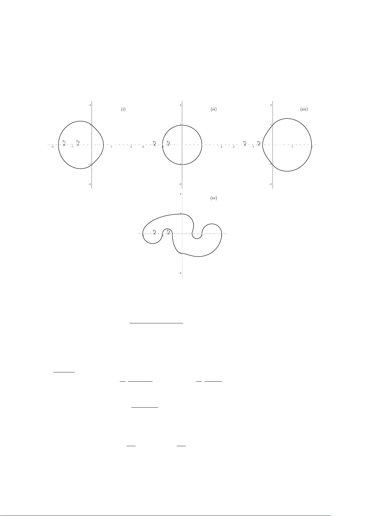
Solving gra vitational ﬁeld equations b y Wiener-Hopf matrix factorisation, and b ey ond M. Cristina Cˆ amara and Gabriel Lop es Cardoso Center for Mathematic al Analysis, Ge ometry and Dynamic al Systems, Dep artment of Mathematics, Instituto Sup erior T´ ecnic o, Universidade de Lisb o a, A v. R ovisc o Pais, 1049-001 Lisb o a, Portugal cristina.camara@tecnico.ulisboa.pt, gabriel.lopes.cardoso@tecnico.ulisboa.pt Abstract By viewing Einstein’s ﬁeld equations – reduced to t w o dimensions – as an integrable sys- tem, one can sim ultaneously obtain exact solutions to b oth the equations themselves and their asso ciated Lax pair via a canonical Wiener–Hopf factorisation of a so-called mon- o drom y matrix. In this article, w e review this remark able interpla y betw een gravitational ﬁeld equations, in tegrable systems, Riemann–Hilbert problems, and Wiener–Hopf factori- sation theory , with particular emphasis on developmen ts from the past decade enabled by adv ances in Wiener–Hopf factorisation techniques arising from the study of singular in tegral equations and T o eplitz operators. Through a v ariet y of concrete examples, we illustrate ho w Wiener–Hopf factorisation yields explicit, exact solutions to the ﬁeld equations of gravita- tional theories, and ho w its generalisation through a so-called τ -in v ariance property pro vides a new solution-generating metho d. Along the w ay , we aim to demonstrate the importance of an interdisciplinary approac h – grounded in General Relativit y , Complex Analysis, and Op erator Theory – for the study of gra vitational ﬁeld equations. 1 In tro duction The study of the in tegrability of Einstein’s ﬁeld equations, and their generalisations to the ﬁeld equations of other gravitational theories, has evolv ed into a sub ject with a long and rich history (see, for instance, [53] and the recent review articles [73, 4, 55]). As emphasized in these reviews, a v ariety of metho ds ha v e b een dev elop ed to searc h for exact solutions of Einstein’s ﬁeld equations, b oth in v acuum and in the presence of a Maxw ell ﬁeld. In the late 1970’s and early 1980’s, several solution generating techniques for the four-dimensional v acuum Einstein ﬁeld equations and Einstein-Maxwell equations were explored - for a survey of exact solutions, see [36, 66]. Man y of these metho ds are based on Gero c h’s observ ation, in his study of the tw o- di- mensional equations go v erning stationary axisymmetric solutions of Einstein’s v acuum ﬁeld equations [33, 34], that each solution is asso ciated with an inﬁnite family of p otentials. F rom these, Gero ch was able to generate, starting from a given ”seed” solution, a family of new so- lutions to the equations. He conjectured that an y stationary , axisymmetric solution could be obtained from Mink owski space-time via an inﬁnite-dimensional group of transformations - a conjecture later pro v en by Ernst and Hauser [40]. How ever, a concrete pro cedure for carrying out these transformations on a giv en ”seed” metric was not pro vided. 1 In a series of pap ers [47, 48, 49, 50], Kinnersley and Chitre succeeded in p erforming these transformations in certain cases, using a 2 × 2 matrix generating function dep ending on W eyl co- ordinates and a complex parameter, whic h w as required to satisfy a system of partial diﬀeren tial equations (PDE’s). In 1978, in a short pap er [58], Maison conjectured that Einstein’s ﬁeld equations in the stationary axially symmetric case constituted a ”completely in tegrable Hamiltonian system”, based on the existence of a linear eigenv alue problem ”in the spirit of Lax”, with the non-linear system of Einstein’s ﬁeld equations app earing as its compatibility condition. Shortly after, Belinski and Zakharov, taking a completely diﬀeren t approac h, prov ed the in tegrability of the v acuum Einstein ﬁeld equations in the presence of tw o comm uting isome- tries [8, 9]. They constructed an ov erdetermined system of linear partial diﬀeren tial equations dep ending on a complex sp ectral parameter τ , as w ell as on tw o of the space-time co ordinates, and demonstrated that Einstein’s ﬁeld equations in v acuum arise as the compatibilit y condition of this linear system. One of the most successful tec hniques for generating exact solutions to Einstein’s ﬁeld equa- tions, pioneered by Belinski and Zakharo v, is the inv erse scattering metho d [1]. In their seminal pap ers [8, 9], they dev elop ed a practical approac h based on a modiﬁed v ersion of the inv erse scattering problem [74, 75]. This method enables the explicit construction of v arious classes of new exact solutions to Einstein’s ﬁeld equations in v acuum in cases where the metric ten- sor depends on only tw o v ariables, pro vided that a ”seed” solution is known. The approac h in volv es solving an asso ciated linear system, assuming the existence of a known solution ψ 0 . A new solution ψ is then constructed via the transformation ψ = χ ψ 0 , where χ is a matrix of a sp eciﬁc form that must b e determined suc h that ψ also satisﬁes the linear system. This requiremen t leads to a new linear system of diﬀerential equations for χ , the solution of whic h reduces to solving a Riemann-Hilbert problem on a certain circle in the complex plane [8]. Once ψ is determined, the corresp onding solution to the original nonlinear Einstein’s ﬁeld equations can b e extracted by ev aluating ψ at τ = 0, where τ is the complex sp ectral parameter. One diﬃculty with the inv erse scattering method, ho wev er, is that it does not necessarily repro duce all the desired features of the solutions – particularly the group structure in models where a symmetry group G acts as a solution generating group [30]. This issue do es not arise in the alternativ e group-theoretical framew ork prop osed b y Breit- enlohner and Maison in [11]. Their aim w as to pro vide a clear group-theoretical understanding of v arious solution generating techniques and to demonstrate that the action of the Gero c h group is directly related to the in v erse scattering metho d developed for completely in tegrable systems. F o cusing on the simplest case, pure Einstein gra vity in four dimensions, they proposed a method for obtaining solutions via a so-called linear sp ectral problem, in whic h Einstein’s ﬁeld equations in v acuum emerge as compatibilit y conditions. This approach also inv olv es solving a sp eciﬁc Riemann-Hilb ert problem and acting with the inﬁnite dimensional Gero ch group on a solution of the linear sp ectral problem. Ho wev er, this me tho d is not easy to implemen t [11, 30, 44, 45, 24, 46]. A completely diﬀeren t metho d to obtaining stationary axisymmetric solutions to Einstein’s ﬁeld equations in v acuum, diﬀeren t from the “B¨ ac klund transformation” approac h often adopted to obtain new solutions to integrable PDE’s [1, 3], is due to W ard in [70]. Motiv ated b y P enrose’s construction for v acuum spaces with self-dual curv ature tensor [63], W ard’s approac h translates the problem in to one of complex geometry , using t wistor theory and a corresp ondence betw een solutions of the ﬁeld equations and complex vector bundles. One wa y to describe v ector bundles is to sp ecify a ”patc hing matrix”, whose elements dep end on a complex v ariable τ as w ell as on the space-time coordinates ( ρ, v ). W ard’s construction 2 consists in ”splitting”, i.e. factorising a 2 × 2 ”patc hing matrix” of the form H ( τ , ρ, v ) =  h 1 ( ω ) ( − τ ) k h 2 ( ω ) τ − k h 2 ( ω ) h 3 ( ω )  with ω = v + ρ 2  1 − τ 2 τ  , k ∈ Z , (1) as H ( τ , ρ, v ) = ˆ H ( τ , ρ, v ) H − 1 ( τ , ρ, v ) , (2) with ˆ H , H non singular, and H analytic with resp ect to τ for | τ | ≤ 1, ˆ H analytic with resp ect to τ for | τ | ≥ 1, including the p oin t ∞ . The solution J ( ρ, v ) of Einstein’s ﬁeld equations in v acuum, written in signature (+ , − , − , − ) in the form ds 2 4 = ρJ ij dy i dy j − Ω( dρ 2 + dv 2 ) , (3) where y 1 , y 2 , ρ, v are the space-time co ordinates, Ω = Ω( ρ, v ) > 0 is a function determined by in tegration once J is known, and J is a symmetric 2 × 2 matrix of real v alued functions of ρ and v with det J = − 1, is then obtained from (2) by the equalit y J = P H (0 , ρ, v ) ˆ H − 1 ( ∞ , ρ, v ) P , (4) where P = diag  ρ − k/ 2 , ρ k/ 2  (see App endix B). The main diﬃcult y in this construction pro cedure, as observed by W ard in [70], is that of ﬁnding the matrices ˆ H and H in the factorisation (2), since there is no systematic pro cedure for obtaining it. Nevertheless, the t wistor approac h to stationary axisymmetric space-times was illustrated b y W ard in several examples, including the Sch warzsc hild solution and the family of Harrison’s metrics [38]. W ard’s pap er was the ﬁrst to recast the stationary axisymmetric v acuum case of Einsteins’s ﬁeld equations as a Rie mann-Hilb ert factorisation problem, without resorting to a previously kno wn ”seed solution” nor to B¨ acklund transformations, and sho wing that v acuum solutions of Einstein’s ﬁeld equations can be view ed as vector bundles ov er related twistor spaces in such a w ay that the space-time metric can b e recov ered from the ”patc hing matrix” by solving a Riemann-Hilb ert factorisation problem. W ard’s twistor analysis of stationary axisymmetric solutions motiv ated m uc h subsequen t w ork following the ideas introduced in his seminal pap er [70]. This approach was further dev elop ed in [71], where the connection to solution-generating tec hniques in General Relativity is explored, and t wistor theory is used to explain the app earance of Riemann-Hilbert problems in the construction of exact solutions. In addition, W ard’s framework was applied to gra vitational w av es with cylindrical symmetry in [72] (see [31] for a review of solutions generated by W ard’s tec hnique). As mentioned ab o v e, linear systems and Riemann-Hilbert problems lie at the core of several metho ds for generating solutions to gra vitational ﬁeld equations. The main diﬃcult y in applying these methods, as emphasized by many authors, see for example [70, 11, 44], lies in solving the asso ciated Riemann-Hilb ert problems – particularly those inv olving factorisations of the t yp e (2) – in a suﬃciently explicit form as to allo w clear information ab out the solution to b e extracted. Ho wev er, recent dev elopmen ts in Riemann-Hilb ert metho ds and adv ances in explicit Wiener- Hopf factorisation tec hniques (including numerical metho ds and RH problems on Riemann surfaces), in connection with the study of T oeplitz op erators [13, 10, 67, 51, 2, 14, 15, 20, 21, 28, 52], hav e allow ed to ov ercome many diﬃculties and to obtain new results and solutions in the past decade. These ha ve not, to the authors’ knowledge, been cov ered in comprehensive 3 surv eys. In this paper w e therefore review how Riemann–Hilb ert problems, in conjunction with Wiener-Hopf matrix factorisation metho ds grounded in complex analysis and op erator theory , can b e employ ed to construct explicit solutions to both the gravitational ﬁeld equations, seen as an in tegrable system, and the underlying linear system. The linear system under consideration is the one introduced in [57], whic h is equiv alen t to the one formulated b y Breitenlohner and Maison in [11]. W e will encounter t w o distinct Riemann-Hilbert problems: one that w e refer to as the R iemann–Hilb ert factorisation pr oblem , and another that w e call the inje ctivity (ve ctorial) R iemann–Hilb ert pr oblem . The latter is obtained by applying results from op erator theory and is crucial in answering the question of existenc e of a canonical Wiener-Hopf factorisation. This review is in tended for researc hers from tw o distinct communities, namely General Relativit y on the one hand, and Complex Analysis and Operator Theory , with an interest in applications in Mathematical Ph ysics, on the other. In addition, by providing explicit examples, w e aim to oﬀer a text that can serve as an in tro duction for graduate students and researchers to the topics discussed in the review and to their in terrelations. Its structure is as follo ws. In Section 2, w e b egin by reviewing the formulation of the gra vitational ﬁeld equations as an in tegrable system. W e introduce the Breitenlohner-Maison linear system, whose formulation in volv es an algebraic curv e called the sp ectral curve. In Section 3 we review Riemann-Hilb ert problems, Wiener-Hopf factorisation tec hniques and deﬁne admissible con tours. W e then discuss ho w canonical Wiener-Hopf factorisations of mono drom y matrices with resp ect to admissible con tours pro vide solutions to b oth the Breitenlohner-Maison linear system as well as to its compatibilit y equations, the gravitational ﬁeld equations. W e illustrate how the canonical fac- torisation of the same monodrom y matrix, with resp ect to diﬀerent admissible contours, can giv e rise to distinct solutions of the gravitational ﬁeld equations. In Section 4 w e turn to a discussion of the existence of a canonical Wiener-Hopf factorisation. This is addressed via the connection with T o eplitz op erators and results from Op erator Theory . As an example, w e discuss the breakdo wn of the existence of a canonical Wiener-Hopf factorisation when approaching the ergosurface of the Kerr black hole of General Relatvity . In Section 5 we discuss a recently in tro- duced solution generation metho d by multiplication, based on an approac h called τ -inv ariance, whic h enables us to go beyond canonical Wiener-Hopf factorisation in constructing solutions of the gravitational ﬁeld equations. W e illustrate this metho d with several examples. Section 6 presents several additional illustrative examples. In Section 7 we form ulate a list of op en questions related to the topics discussed in this review. Finally , App endix A provides a short in tro duction to T o eplitz op erators and Wiener-Hopf factorisation, and is intended primarily to pro vide the necessary bac kground results for readers who are not familiar with these topics, while in App endix B w e compare W ard’s factorisation approach with the canonical Wiener-Hopf factorisation framework. 2 The gra vitational ﬁeld equations as an in tegrable system The ﬁeld equations of gravitational theories in D space-time dimensions are a system of non- linear partial diﬀeren tial equations (PDE’s) for the space-time metric (and p ossibly other ﬁelds) for which obtaining exact solutions is, in general, a diﬃcult task. Exact solutions can, ho wev er, b e obtained under simplifying assumptions, such as imp osing spherical symmetry . One w ell- kno wn example of such a solution, whic h holds signiﬁcan t ph ysical and mathematical in terest, is the Sch warzsc hild solution. Solutions to the gravitational ﬁeld equations, also known as Einstein’s ﬁeld equations in the context of General Relativity , can b e formulated in v arious co ordinate systems. Here, w e fo cus on a speciﬁc subset of solutions to these ﬁeld equations that exhibit a suﬃcien t num b er of 4 comm uting isometries, enabling a dimensional reduction of the problem to tw o dimensions. By p erforming a t w o-step dimensional reduction of the original theory (which w e assume to hav e a v anishing cosmological constant), this leads to a system of non-linear, second-order PDEs [11, 57, 61, 65] that dep end on tw o co ordinates, whic h w e tak e to b e the W eyl co ordinates ρ, v (with ρ > 0 , v ∈ R ): d ( ρ ⋆ A ) = 0 , with A = M − 1 dM , M = M ( ρ, v ) , (5) where M ∈ G/H is a coset representativ e of the symmetric space G/H that arises in the t wo- step reduction, and we assume det M = 1. In (5), ⋆ denotes the Ho dge star op erator in t w o dimensions, satisfying ⋆dρ = − λ dv , ⋆dv = dρ , ( ⋆ ) 2 = − λ id , (6) where λ = ± 1, dep ending on the form of the tw o-dimensional line elemen t ds 2 2 = σ dρ 2 + εdv 2 , (7) with σ, ε = ± 1 , λ = σ ε . Note that A satisﬁes dA + A ∧ A = 0 . (8) The symmetric space G/H is inv arian t under an inv olution called gener alise d tr ansp osition , whic h w e denote by ♮ , determined by the gra vitational mo del under consideration. Hence M ♮ = M . F or 2 × 2 matrices, ♮ coincides with matrix transp osition. Examples of gravitational theories in D dimensions and their asso ciated symmetric spaces G/H are: • D = 4 Einstein gravit y: G/H = S L (2 , R ) /S O (1 , 1) or S L (2 , R ) /S O (2) • D = 4 Einstein + Maxwell theory: G/H = S U (2 , 1) / ( S L (2 , R ) × U (1)) or S U (2 , 1) / ( S U (2) × U (1)) • D = 5 Einstein gravit y: G/H = S L (3 , R ) /S O (2 , 1) or S L (3 , R ) /S O (3) When D = 4, the asso ciated four-dimensional space-time metric takes the W eyl-Lewis- P apap etrou form, ds 2 4 = − λ ∆( dy + B dϕ ) 2 + ∆ − 1  e ψ ds 2 2 + ρ 2 dϕ 2  , (9) where ∆( ρ, v ) , B ( ρ, v ) are determined b y the solution M ( ρ, v ) of (5). F or instance, in the case of Einstein’s ﬁeld equations in v acuum, we hav e that the matrix M ( ρ, v ) is a symmetric 2 × 2 matrix of determinant 1 giv en b y [11] M =  ∆ + ˜ B 2 / ∆ ˜ B / ∆ ˜ B / ∆ 1 / ∆  , with ρ ⋆ d ˜ B = ∆ 2 dB . (10) ψ ( ρ, v ) is a scalar function determined by in tegration [57, 65] from ∂ ρ ψ = 1 4 ρ T r  A 2 ρ − λ A 2 v  , ∂ v ψ = 1 2 ρ T r ( A ρ A v ) . (11) 5 Note that, in (11), ∂ v ( ∂ ρ ψ ) = ∂ ρ ( ∂ v ψ ), as can b e veriﬁed b y using (5) and (6). F or examples of W eyl metrics in dimensions D > 4, see [29]. The non-linear ﬁeld equations (5) constitute an integrable system [7, 42], i.e. they app ear as a compatibility condition for an asso ciated linear system of PDE’s, called a Lax pair, that in volv es, b esides the space-time co ordinates ρ, v , a complex parameter τ , called the sp e ctr al p ar ameter . The Lax pair takes the form [57] τ ( dX ( τ , ρ, v ) + A ( ρ, v ) X ( τ , ρ, v )) = ⋆ dX ( τ , ρ, v ) , (12) where the sp ectral parameter τ v aries on a sp ectral curve giv en by ω = v + λ 2 ρ λ − τ 2 τ . (13) This linear system (for the unkno wn matrix X ( τ , ρ, v )) will be called the Breitenlohner-Maison linear system [11]. 1 Omitting, for simplicit y , the dependence on the spectral parameter and the W eyl co ordinates, the Lax pair (12) b ecomes τ ( dX + AX ) = ⋆ dX . (14) The complex parameter τ plays a crucial role here in allowing to bring in the to ols of complex analysis and in reform ulating the problem of obtaining solutions to (5) in terms of a Riemann-Hilb ert problem, as we shall explain in Section 3. Note that the sp ectral relation (13) is inv ariant under the inv olution i λ ( τ ) = − λ τ , τ ∈ C \{ 0 } . (15) As a consequence, the relation (13) will b e satisﬁed if we replace τ by an y of the functions φ ± ω ( ρ, v ) = − λ ( ω − v ) ± p ( ω − v ) 2 + λρ 2 ρ , (16) where φ − ω = − λ/φ + ω , as can b e easily v eriﬁed. W e denote the class of all functions of the form (16) by T . The integrabilit y of the non-linear ﬁeld equations (5) can th us b e expressed as follows, using the notation deﬁned ab ov e. Theorem 2.1. [57] [5, The or em 4.2] L et φ ∈ T . If, for a given A = M − 1 dM , ther e exists X ( τ , ρ, v ) such that up on substituting τ = φ , we have X ∈ C 2 , X − 1 ∈ C 1 and τ ( dX + AX ) = ⋆ dX , (17) then M is a solution to (5) . Note, ho w ever, that although the Breitenlohner–Maison linear system (14) is formally a system of linear PDE’s for the unkno wn X , with coeﬃcient A ( ρ, v ), it should in fact b e viewed as a system of equations for the pair of unkno wns ( X , A ). This is because A is not given a priori; rather, our goal is to determine a 1-form A = M − 1 dM such that (5) holds. In the next section we will review ho w this can b e achiev ed by solving a Riemann-Hilb ert problem whic h yields b oth a solution M ( ρ, v ) to the ﬁeld equations (5) and a solution X to the Breitenlohner–Maison linear system (14) with input A = M − 1 dM . 1 W e presen t it here in the form given in [57]. Other equiv alen t linear systems ma y be considered, see [61, 30, 44] for a detailed analysis of their mutual relations. 6 3 Solving the ﬁeld equations b y canonical Wiener-Hopf factori- sation W e begin by brieﬂy reviewing the Riemann-Hilb ert (RH) problems that we will consider here, along with the related concept of Wiener-Hopf factorisation. Let Γ ⊂ C b e a closed con tour, i.e., a simple closed path in the complex τ -plane [69], and let M ( τ ) b e an n × n matrix function, which w e assume to b e H¨ older con tinuous [59, 25], deﬁned on Γ. A RH problem with coeﬃcient M consists in ﬁnding matrix v alued (or v ector v alued) Φ + and Φ − , belonging to certain classes of functions analytic in the in terior and the exterior of Γ, resp ectively , suc h that M ( τ ) Φ + ( τ ) = Φ − ( τ ) on Γ . (18) This can b e a matricial, ve ctorial or sc alar pr oblem. A particularly important type of RH problems arises in the context of matrix factorisation. By a Wiener-Hopf (WH) factorisation of a matrix M ( τ ) as abov e, w e mean a representation of the form M = M − D M + on Γ , (19) where M ± 1 + are analytic and bounded in the in terior of Γ (denoted int Γ), M ± 1 − are analytic and b ounded in the exterior of Γ (denoted ext Γ), and D is a diagonal matrix of the form D = diag( τ k 1 , . . . , τ k n ), with k i ∈ Z . It is w ell kno wn [59] that any inv ertible H¨ older con tin uous matrix admits a factorisation of the form (19). If k j = 0 ( j = 1 , . . . , n ), then we ha ve M = M − M + , (20) whic h is called a c anonic al WH factorisation. Note that, since, for any in vertible constan t matrix K , w e ha ve that M = ( M − K )  K − 1 M +  is also a canonical WH factorisation, we can normalise M + so that M + (0) = I n × n , where I n × n denotes the identit y matrix. Clearly , obtaining suc h a factorisation is equiv alent to solving a particular RH problem of the form M M − 1 + = M − . (21) Remark 3.1. Note that, for a RH problem to b e well form ulated, one must sp ecify b oth the class of analytic functions in which the solutions are sough t, and the closed contour Γ with resp ect to whic h the RH problem is formulated. Consequently , RH problems with the same co eﬃcien t M ( τ ) ma y hav e diﬀeren t solutions, dep ending on the c hoice of the solution class and the closed contour. Here w e will b e considering admissible c ontours , deﬁned as simple closed paths encircling the origin and inv ariant under the in v olution i λ ( τ ) = − λ τ . W e will also only be considering matrices that dep end on a particular combination of the complex v ariable τ and the W eyl co ordinates ρ, v , resulting from the comp osition of a matrix function M ( ω ) with the spectral relation (13), i.e. of the form M ρ,v ( τ ) = M  v + λ 2 ρ λ − τ 2 τ  , (22) where ρ, v pla y the role of parameters as far as the RH problem is concerned. W e assume moreo ver that det M ( ω ) = 1 and M ♮ ( ω ) = M ( ω ). Such matrices are called mono dr omy matric es. They pla y the role of “patching matrices” in W ard’s construction. 2 2 The name mono dromy matrix has its origin in the relationship of the theory of isomono dromic deformations with Einstein’s ﬁeld equations [54, 55]. 7 Canonical Wiener-Hopf factorisation of mono dromy matrices with resp ect to an admis- sible con tour provides a metho d for obtaining a pair ( X , A ), where X is a solution to the Breitenlohner-Maison linear system (14) with input A , and A is a solution to the non-linear ﬁeld equations (5). The follo wing result w as obtained in [5], and it holds under v ery general conditions. Here w e present it in a slightly simpliﬁed form (omitting certain standard diﬀeren- tiabilit y assumptions with resp ect to ρ and v ; for further details, see [5]). Theorem 3.2. [5, The or em 6.1] L et Γ b e an admissible c ontour. L et M ρ,v ( τ ) b e analytic, as wel l as its inverse, in a neighb ourho o d of Γ , and admitting a c anonic al WH factorisation with r esp e ct to Γ , M ρ,v ( τ ) = ( M ρ,v ) − ( τ ) ( M ρ,v ) + ( τ ) on Γ , (23) wher e ( M ρ,v ) + (0) = I n × n ∀ ρ, v . (24) Then lim τ →∞ ( M ρ,v ) − ( τ ) = M ( ρ, v ) (25) satisﬁes the ﬁeld e quations (5) and X ( τ , ρ, v ) := ( M ρ,v ) + ( τ ) , with τ = φ ∈ T , is a c orr esp ond- ing solution to the line ar system (14) . Remark 3.3. Note that, since M ♮ ( ω ) = M ( ω ) and M ρ,v ( τ ) is obtained as in (22), one can pro ve [11, 44, 17] that, if M ρ,v ( τ ) admits a canonical WH factorisation of the form (23), with ( M ρ,v ) + ( τ ) normalised as in (24) and denoted X ( τ , ρ, v ), then one can rewrite the factor ( M ρ,v ) − ( τ ) in such a w ay that the canonical factorisation b ecomes M ρ,v ( τ ) = X ♮  − λ τ , ρ, v  M ( ρ, v ) X ( τ , ρ, v ) . (26) Note that diﬀer ent solutions may b e obtained from the same mono dr omy matrix if one c ho oses diﬀer ent admissible c ontours Γ with resp ect to whic h the factorisation is p erformed . Therefore the mono dromy matrix does not contain all the information regarding the solutions; there is an added information in the chosen con tour, in line with what w e mentioned in Remark 3.1. Consider the following example. Example 3.4. T ake the Sc hw arzschild monodromy matrix, obtained from M ( ω ) =  λ ω − m ω + m 0 0 λ ω + m ω − m  , m ∈ R + , (27) b y composition with the spectral relation (13) with λ = 1 (w e refer to [5] for a detailed discussion of the tw o cases λ = ± 1). The resulting mono drom y matrix is M ρ,v ( τ ) = " ( τ − τ 1 )( τ +1 /τ 1 ) ( τ − τ 2 )( τ +1 /τ 2 ) 0 0 ( τ − τ 2 )( τ +1 /τ 2 ) ( τ − τ 1 )( τ +1 /τ 1 ) # , (28) where τ 1 = τ 1 ( ρ, v ) = v − m − q ( v − m ) 2 + ρ 2 ρ , τ 2 = τ 2 ( ρ, v ) = v + m − q ( v + m ) 2 + ρ 2 ρ . (29) 8 There are four p ossible classes of admissible contours from which Γ can b e chosen, dep ending on whic h of the p oin ts τ 1 and τ 2 are inside or outside Γ. Note that, since Γ must b e inv ariant under the inv olution τ 7→ − 1 /τ , it has t w o ﬁxed p oin ts, ± i , and if τ ∈ int Γ then − 1 /τ ∈ ext Γ. Moreo ver, M ρ,v m ust b e con tin uous on Γ, so none of the p oints τ i , − 1 /τ i ( i = 1 , 2) belong to Γ. The four types of admissible contours are depicted in Figure 1 for the case when − m < v < m , in which case w e ha ve that τ 1 < − 1 < τ 2 < 0. - 2 - 1 1 2 - 2 - 1 1 2 - 2 - 1 1 2 - 2 - 1 1 2 - 2 - 1 1 2 - 2 - 1 1 2 - 2 - 1 1 2 - 2 - 1 1 2 Figure 1: − m < v < m : four distinct choices of con tours. F actorising with resp ect to Γ we obtain, in eac h case, a canonical WH factorisation, ( τ − τ 1 ) ( τ + 1 /τ 1 ) ( τ − τ 2 ) ( τ + 1 /τ 2 ) = m − ( τ ) m + ( τ ) , (30) whic h yields M ( ρ, v ) =  m − ( ∞ ) 0 0 m − 1 − ( ∞ )  =  ∆ 0 0 ∆ − 1  . (31) (i) Case 1: m + ( τ ) = τ 1 τ 2 τ + 1 /τ 1 τ + 1 /τ 2 , m − ( τ ) = τ 2 τ 1 τ − τ 1 τ − τ 2 , ∆ = τ 2 /τ 1 , (32) yielding a solution which, under the change of coordinates ρ = p r 2 − 2 mr sin θ , v = ( r − m ) cos θ , (33) results in the four-dimensional line elemen t ds 2 4 = −  1 − 2 m r  dt 2 +  1 − 2 m r  − 1 dr 2 + r 2  dθ 2 + sin 2 θ dϕ 2  . (34) 9 Th us, the solution describ es the exterior r e gion of the Schwarzschild black hole . (ii) Case 2: m + ( τ ) = 1 τ 1 τ 2 τ − τ 1 τ + 1 /τ 2 , m − ( τ ) = τ 1 τ 2 τ + 1 /τ 1 τ − τ 2 , ∆ = τ 1 τ 2 , (35) yielding a solution which, under the change of coordinates ρ = p 2 mϱ − ϱ 2 sinh ϑ , v = ( ϱ − m ) cosh ϑ , (36) with ϱ ∈ ]0 , 2 m [ , ϑ ∈ ]0 , ∞ [, yields the four-dimensional line element ds 2 4 =  1 − 2 m ϱ  dt 2 −  1 − 2 m ϱ  − 1 dϱ 2 + ϱ 2  dϑ 2 + sinh 2 ϑ dϕ 2  , (37) whic h is an example of an AI I -metric [36]. (iii) Case 3: m + ( τ ) = τ 2 τ 1 τ − τ 1 τ − τ 2 , m − ( τ ) = τ 1 τ 2 τ + 1 /τ 1 τ + 1 /τ 2 , ∆ = τ 1 /τ 2 , (38) yielding a solution which, under the change of coordinates ρ = p r 2 + 2 mr sin θ , v = ( r + m ) cos θ , (39) results in the four-dimensional line elemen t ds 2 4 = −  1 + 2 m r  dt 2 +  1 + 2 m r  − 1 dr 2 + r 2  dθ 2 + sin 2 θ dϕ 2  . (40) This is the ‘negativ e mass’ Sch warzsc hild solution [36], whic h has a nak ed curv ature singularity at r = 0. (iv) Case 4: m + ( τ ) = τ 1 τ 2 τ + 1 /τ 1 τ − τ 2 , m − ( τ ) = 1 τ 1 τ 2 τ − τ 1 τ + 1 /τ 2 , ∆ = 1 τ 1 τ 2 . (41) This is analogous to Case 2 and yields the same solution upon using the transformation v 7→ − v , whic h induces the transformation τ 1 τ 2 7→ 1 / ( τ 1 τ 2 ). 4 Canonical Wiener-Hopf factorisation: the question of exis- tence Theorem 3.2 presupposes the existence of a canonical WH factorisation of the mono dromy matrix M ρ,v ( τ ). But do es such a factorisation actually exist? This is a natural and imp ortan t question, raised by sev eral authors, see for example [70, 11, 44]. Indeed, for any inv ertible H¨ older con tin uous matrix function, a WH factorisation of the form (19) alwa ys exists, but, in general, it will not be canonical, i.e. we do not hav e k i = 0 for all i . Even in the case of scalar functions, the factorisation is canonical only if the winding n umber of the function around the origin is zero [35, 25, 59]; for example, a simple function like f ( τ ) = τ do es not admit a canonical WH factorisation. Therefore, what follo ws is a surprising result: although simple in form, it reveals that functions dep ending on τ via comp osition with the sp ectral relation, as in (22), hav e very special prop erties. 10 Theorem 4.1. [22] L et g b e a sc alar H¨ older c ontinuous function on an admissible c ontour Γ and let g ρ,v ( τ ) = g  v + λ 2 ρ λ − τ 2 τ  b e non-vanishing on Γ . Then g ρ,v ( τ ) admits a c anonic al factorisation. The canonical factorisation of g ρ,v ( τ ) in the ab ov e theorem can b e explicitly obtained using the complementary pro jections P ± Γ = 1 2 (Id ± S Γ ) , (42) where Id denotes the iden tity op erator and S Γ is the singular in tegral op erator with Cauch y k ernel deﬁned b y (see App endix A) ( S Γ φ ) ( τ ) = 1 π i P . V . ˆ Γ φ ( u ) u − τ du , τ ∈ Γ . (43) S Γ maps the space C µ Γ of all H¨ older con tin uous functions (on Γ) with exp onent µ ∈ ]0 , 1[ onto itself [59, 25]. W e then ha ve g ρ,v ( τ ) = ( g ρ,v ) − ( τ ) ( g ρ,v ) + ( τ ) (44) with ( g ρ,v ) ± = e P ± Γ log g ρ,v . (45) Theorem 4.1 has signiﬁcan t consequences, in particular the following, whic h is a consequence of well kno wn results in the theory of WH factorisation [25, Chapter 4], [56, 59]. Corollary 4.2. L et Γ b e an admissible c ontour and let M ρ,v ( τ ) , deﬁne d as in (22) , b e in  C µ Γ  n × n , with non-vanishing determinant on Γ . (i) If M ρ,v ( τ ) is diagonal, then it admits a c anonic al WH factorisation that c an b e explicitly obtaine d by factorising e ach diagonal element ac c or ding to (44) and (45) . (ii) If M ρ,v ( τ ) c an b e r e duc e d to triangular form by left multiplic ation with a matrix that is analytic and b ounde d in ext Γ , along with its inverse, and right multiplic ation with a matrix that is analytic and b ounde d in in t Γ , along with its inverse, then M ρ,v ( τ ) admits a c anonic al factorisation. F or matrix functions whic h do not satisfy the conditions of Corollary 4.2, the question of whether they admit a canonical factorisation may be considerably more complex. T o address it, w e will use the close relationship b etw een WH factorisation and the study of T o eplitz operators (see Appendix A for a v ery brief introduction to this topic). The latter are compressions of m ultiplicative op erators into the Hardy space H 2 + = P + Γ L 2 (Γ) (where L 2 (Γ) denotes the space of all square-integrable functions on Γ), or its v ectorial analogues  H 2 +  n in the matricial case. Concretely , given an n × n matrix function G whose elemen ts are b ounded functions on Γ, the T o eplitz op erator T G is deﬁned by T G = P + Γ GP + Γ | ( H 2 + ) n : ( H 2 + ) n → ( H 2 + ) n , (46) where ( H 2 + ) n is the space of n × 1 vectorial functions with elemen ts in H 2 + and P + Γ is the pro jection deﬁned in (42), applied comp onent wise. G is called the symb ol of the T o eplitz op erator. The connection with WH factorisation comes from the following results presen ted in more detail in App endix A. 11 Theorem 4.3. If G is an invertible H¨ older c ontinuous matrix function deﬁne d on Γ , then G admits a c anonic al WH factorisation if and only if the T o eplitz op er ator with symb ol G , deﬁne d in (46) , is invertible. Theorem 4.4. With the same assumptions as in The or em 4.3, if det G = 1 then T G is invert- ible in  H 2 +  n if and only if it is inje ctive. No w, it follows from the deﬁnition of a T o eplitz op erator and from the complemen tarity of the pro jections P + Γ and P − Γ deﬁned in (42) that T G is injectiv e (i.e. ker T G = { 0 } ) if and only if the only solution to the vectorial RH problem G Ψ + = Ψ − , Ψ ± ∈  H 2 ±  n (47) is the trivial solution Ψ ± = 0, where H 2 ± = P ± Γ L 2 (Γ) . (48) W e call the RH problem (47) the inje ctivity RH pr oblem for the T o eplitz op erator T G . Th us, w e ha ve the follo wing. Prop osition 4.5. With the same assumptions as in The or em 4.3, with det G = 1 , G has a c anonic al factorisation if and only if (47) admits only the trivial solution. Note that although (47) and the RH factorisation problem (21) ha ve a similar form, they are in fact quite diﬀerent, since in (47) one lo oks for vectorial solutions in  H 2 ±  n , in particular with Ψ − ( ∞ ) = 0, while in (21) the solutions are sought in the space of n × n matrix functions whic h are analytic and b ounded either in the exterior or in the interior of Γ (see Remark 3.1). Indeed, these tw o RH problems address diﬀerent questions: by solving (47) w e determine the kernel of T G and answ er the question of whether or not there exists a canonical WH factorisation, while the solution to (21) pro vides that factorisation, if it exists. Also note that the existence of a canonical factorisation is stable under small perturbations, as is well kno wn (see Appendix A). F or rational matrices, it is, in principle, alw ays possible to determine whether the asso ciated injectivit y RH problem admits only the zero solution. In practise, how ev er, this can b e a highly non trivial task. It is imp ortan t to note that the kno wn results for general rational matrices [25, 59, 56] cannot b e directly applied in our setting, due to the sp eciﬁc dep endence of the mono drom y matrices on τ , as made evident b y Theorem 4.1 and Corollary 4.2. Ho wev er, for 2 × 2 rational matrices obtained as in (22) from M ( ω ) = 1 q ( ω )  p 11 ( ω ) p 12 ( ω ) p 12 ( ω ) p 22 ( ω )  , (49) where q , p 11 , p 12 , p 22 denote p olynomials of degree n, k 11 , k 12 , k 22 , resp ectively , and where we assume that q only has simple zero es, and furthermore denoting N 1 = max { k 11 , k 12 } , N 2 = max { k 12 , k 22 } , (50) w e ha ve the follo wing simple criteria. Theorem 4.6. [19, The or em 3.5] With the notation ab ove and M ρ,v ( τ ) given by (22) , let Γ b e an admissible c ontour wher e det M ρ,v ( τ ) = 1 . Then we have: 12 (i) if N 1 + N 2 < 2 n , then M ρ,v ( τ ) has a c anonic al WH factorisation w.r.t. Γ , for al l ρ, v ; (ii) if N 1 + N 2 = 2 n , then M ρ,v ( τ ) has a c anonic al WH factorisation w.r.t. Γ for al l ρ, v , exc ept for the p oints on a c ertain curve C in the Weyl plane; (iii) the c ase wher e N 1 + N 2 > 2 n c an b e r e duc e d to c ase (ii). T o exemplify this result and illustrate how the curv e C , along which the canonical WH factorisation of M ρ,v ( τ ) breaks down, is determined, we consider the follo wing. Example 4.7. The Kerr black hole (with λ = 1) Consider the non-extremal Kerr matrix (see [71, 73, 44]) M ( ω ) = 1 ω 2 − c 2  ( ω − m ) 2 + a 2 2 am 2 am ( ω + m ) 2 + a 2  , c = p m 2 − a 2 > 0 . (51) The corresp onding matrix M ρ,v ( τ ) is given b y M ρ,v ( τ ) = τ 2 q 4 ( τ ) ˜ M ρ,v ( τ ) , (52) where q 4 ( τ ) = 1 4  ρ 2 (1 − τ 2 ) 2 + 4( v 2 − c 2 ) τ 2 + 4 ρv τ (1 − τ 2 )  , ˜ M ρ,v ( τ ) = ( v − m + ρ (1 − τ 2 ) 2 τ ) 2 + a 2 2 am 2 am ( v + m + ρ (1 − τ 2 ) 2 τ ) 2 + a 2 ! . (53) Note that this corresp onds to the case considered in Theorem 4.6 ( ii ) , with n = 2 , k 11 = k 22 = 2 , k 12 = 0 , N 1 = N 2 = 2 , 2 n = 4 = N 1 + N 2 . No w let τ 1 = v − c − p ( v − c ) 2 + ρ 2 ρ , τ 2 = v + c − p ( v + c ) 2 + ρ 2 ρ . (54) Solving the injectivit y RH problem (47) by means of a generalisation of Liouville’s theorem [17, Lemma, Section 3] one obtains an algebraic homogeneous linear system of four equations for four unknown constants, that can b e solv ed by Cramer’s rule; the determinant D ( ρ, v ) of that linear system m ust be diﬀeren t from zero for the only solution to b e zero (see [19] for details on the calculation). Th us M ρ,v ( τ ) will ha v e a canonical factorisation if and only if ( ρ, v ) do es not lie on the curve deﬁned b y D ( ρ, v ) = 0, which can b e shown in this case to b e equiv alen t to − 16( m − v ) 2 τ 2 1 τ 2 2 + ρ 2  1 + 4 τ 3 1 τ 2 + 6 τ 2 1 τ 2 2 + 4 τ 1 τ 3 2 + τ 4 1 τ 4 2  − 8 ρ ( m − v ) τ 1 τ 2  − τ 1 − τ 2 + τ 2 1 τ 2 + τ 1 τ 2 2  = 0 . (55) This condition describ es a curv e C in the W eyl half-plane of the coordinates ρ > 0 , v ∈ R . If w e express (55) in terms of prolate spheroidal co ordinates ( u, y ) (see [37, 44]), v = u y , ρ = p ( u 2 − c 2 )(1 − y 2 ) , (56) where c < u < + ∞ , | y | < 1 , (57) w e obtain from (55) u ( y ) = p m 2 − a 2 y 2 . (58) 13 This equation deﬁnes the ergosurface of the non-extremal Kerr black hole in four dimensions, in the exterior region, where the metric comp onent g tt of the Kerr metric v anishes. The curve C deﬁned b y (55) is represented in Figure 2, in the W eyl half-plane. The region b et w een the curve C and the axis ρ = 0 represen ts the ergosphere (the region betw een the ergo- surface C and the outer horizon of the non-extremal Kerr blac k hole), while the complementary region describ es the region outside the ergosphere. - 1.5 - 1.0 - 0.5 0.5 1.0 1.5 0.2 0.4 0.6 0.8 1.0 Figure 2: Curv e C in the W eyl co ordinates upper half-plane ( ρ > 0 , v ) for the v alues m = 2 , a = 1. The horizon tal axis represen ts v ∈ R , while the vertical axis represen ts ρ > 0. 5 Bey ond Wiener-Hopf factorisation: τ -in v ariance and solution generation b y m ultiplication The question of existence of a canonical factorisation was addressed in Section 4. How ever, ev en when such a factorisation exists, t w o further questions naturally arise. The ﬁrst concerns the explicit construction of a canonical WH factorisation. F or matrix functions, this alw ays dep ends on their sp eciﬁc form and requires the dev elopment of tailored metho ds for diﬀerent classes of matrices [42]. Recen t adv ances in this area ha ve made it p ossible to apply new factorisation tec hniques to a v ariety of matrix classes. W e present tw o examples in Section 6. The second question is whether an y solution to (5) can b e obtained from a canonical WH factorisation of an asso ciated mono dromy matrix, as describ ed in Section 4. The answer to this second question is in the negative, as the following example demonstrates. Example 5.1. Consider the cosmological Kasner solution to Einstein’s ﬁeld equations in four dimensions, ds 2 4 = − dt 2 + 3 X i =1 t 2 p i dx 2 i , 3 X i =1 p i = 1 , 3 X i =1 p 2 i = 1 , (59) with p 1 = p 3 = 2 3 , p 2 = − 1 3 , (60) whic h is of the form (9) with λ = − 1. The corresp onding W eyl-Lewis-Papapetrou form of the line element is ds 2 4 =  ρ 2  4 dy 2 + 9 4  ρ 2  4  dv 2 − dρ 2  +  2 ρ  2 dϕ 2 , (61) where ρ = 2 t 1 / 3 , v = 2 3 x 1 , y = x 3 , ϕ = 1 2 x 2 . (62) 14 In this case, we ha ve that M ( ρ, v ) actually only dep ends on ρ [5], M ( ρ, v ) = M ( ρ ) =  ρ 2  4 0 0  ρ 2  − 4 ! . (63) Due to the particularly simple form of M ( ρ, v ), one can explicitly solv e the Breitenlohner-Maison linear system (14) with co eﬃcien t A = M − 1 dM , which results in the general solution X ( τ , ρ, v ) = τ 2 ρ 2 c 1 τ 2 ρ 2 c 2 ρ 2 τ 2 c 3 ρ 2 τ 2 c 4 ! , (64) where c i , i = 1 , . . . , 4 are arbitrary integration constan ts. It is clear, on the one hand, that the matrix function X cannot b e normalised to the iden tity at τ = 0, so it cannot b e a factor in a canonical WH factorisation. On the other hand, the pro duct (26), for any matrix of the form (63), is a constant matrix in volving only the v alues of c i , i = 1 , . . . , 4, so in this case it is not possible to construct a meaningful mono drom y matrix which w ould, by canonical WH factorisation, provide a solution to the linear system (see Remark 3.3). It is thus natural to lo ok for new approaches - extending b ey ond, but still including, the Wiener–Hopf factorisation framework - that allow to construct other classes of solutions. A motiv ation for generalising the Riemann-Hilb ert method to solving (5), as des crib ed in Theorem 3.2, comes from the structure of its proof presented in [5]. That pro of relies in a crucial wa y on showing that the factor X in a canonical WH factorisation of M ρ,v ( τ ) satisﬁes a boundary v alue problem on Γ, which is not a Riemann-Hilb ert problem (see eq. (6.17) in [5]). This leads to the conclusion that a certain expression inv olving X and its deriv atives, of the form G M ,X ( τ , ρ, v ) = τ dM + 1 ρ  ( λ − τ 2 ) dρ + 2 λτ dv  M ∂ X ∂ τ X − 1 + τ 2 + λ τ M  ∂ X ∂ ρ dρ + ∂ X ∂ v dv  X − 1 , (65) is indep endent of the sp ectral parameter τ . Remark ably , this prop ert y , b y itself and without in volving an y prior factorisation of a mono drom y matrix, leads to the desired conclusion, as stated in the following result. Theorem 5.2. [18, The or em 3.3] L et Γ b e an admissible c ontour and let X ( τ , ρ, v ) and M ( ρ, v ) b e matrix functions such that X ± 1 ar e analytic with r esp e ct to τ in a neighb ourho o d of Γ for al l ( ρ, v ) , and X ± 1 , M ar e of class C 2 with r esp e ct to ( ρ, v ) , and M = M ♮ . L et G M ,X ( τ , ρ, v ) b e deﬁne d by (65) , wher e we omitte d the dep endenc e of X and M on ( τ , ρ, v ) and ( ρ, v ) , r esp e ctively, on the right hand side for simplicity. If, for al l ( ρ, v ) , ∂ ∂ τ G M ,X ( τ , ρ, v ) = 0 on Γ , (66) then M ( ρ, v ) is a solution to the ﬁeld e quation (5) and X ( τ , ρ, v ) , with τ = φ ∈ T , is a solution to the line ar system (14) . W e refer to (66) as the prop erty of τ -in v ariance. It is natural to ask ho w one can explicitly construct matrices X and M that satisfy the assumptions of Theorem 5.2 and for which (66) holds. It follows from the pro of of Theorem 15 3.3 in [5] that any pair of functions X ( τ , ρ, v ) and M ( ρ, v ), obtained from a canonical WH factorisation of a mono drom y matrix, will do; but, just as there are no general metho ds to obtain the WH factorisation of a matrix function, there is also no systematic pro cedure to obtain functions X and M satisfying (66). Nev ertheless, by using the fact that, for an y ω i ∈ C (with ω i  = v ), if τ i , ˜ τ i = − λ/τ i are the t wo ro ots of the equation ω i = v + λ 2 ρ λ − τ 2 τ , (67) w e ha ve  τ − ˜ τ i τ − τ i  − 1 = τ i ˜ τ i − λ τ − ˜ τ i − λ τ − τ i , (68) w e can c haracterise a class of functions satisfying the conditions of Theorem 5.2, whic h are not obtained from the canonical WH factorisation of a mono drom y matrix. W e hav e the follo wing. Prop osition 5.3. [18, Pr op osition 3.6] L et ω i , τ i , ˜ τ i b e deﬁne d as ab ove. L et R i ( τ , ρ, v ) = τ i ˜ τ i τ − ˜ τ i τ − τ i , N i ( ρ, v ) = ˜ τ i τ i = − λ τ 2 i = − λ ˜ τ 2 i , i = 1 , . . . , n , (69) and R ( τ , ρ, v ) = diag ( R α i ( τ , ρ, v )) i =1 ,...,n , N ( ρ, v ) = diag ( N α i ( ρ, v )) i =1 ,...,n , (70) with α ∈ R . Then R ( τ , ρ, v ) and N ( ρ, v ) satisfy ∂ ∂ τ G R,N ( τ , ρ, v ) = 0 (71) on any admissible c ontour Γ such that τ i , ˜ τ i / ∈ Γ for al l i = 1 , . . . , n . Corollary 5.4. [18, Cor ol lary 3.7] With the same assumptions as in The or em 5.2, N ( ρ, v ) deﬁne d in (70) yields a solution to the ﬁeld e quations (5) . Moreo ver, as w e sho w next, we c an use the functions deﬁned in Theorem 5.2 to generate new families of solutions by multiplication, provided that certain comm utation relations inv olving b oth the solutions to (5) and the corresp onding solutions to the linear system (14) hold. In what follo ws we denote b y F the class of all pairs ( M , X ) of matrices X = X ( τ , ρ, v ) , M = M ( ρ, v ) satisfying the assumptions of Theorem 5.2 and such that (66) holds. W e hav e the following. Theorem 5.5. [18, The or em 3.9] L et Γ b e an admissible c ontour and let ( N , R ) , ( M , X ) ∈ F . Then, if R c ommutes with X and its derivatives with r esp e ct to τ , ρ, v , M c ommutes with R and its derivatives with r esp e ct to τ , ρ, v , and N c ommutes with X and its derivatives with r esp e ct to τ , ρ, v , we have that RX is a solution to the line ar system (14) , with τ = φ ∈ T , for the c o eﬃcient A = ( M N ) − 1 d ( M N ) , and ( M N )( ρ, v ) is a solution to the ﬁeld e quations (5) . 16 Remark 5.6. The comm utation relations in Theorem 5.5 hold, in particular, for diagonal ma- trices. As concrete examples of the solution generating metho d presented in Theorem 5.5 w e obtain ﬁrst a cosmological Kasner solution from the interior region of the Sc hw arzschild solution using matrices N deﬁned in Prop osition 5.3, then the solution of Example 5.1 and, ﬁnally , w e show ho w to tak e adv antage of some remark able prop erties of Einstein-Rosen wa v es to obtain a family of deformations of a Kasner solution. Example 5.7. Consider the Sch w arzsc hild mono dromy matrix obtained from (27) b y substi- tuting ω = v + λ 2 ρ λ − τ 2 τ with λ = − 1. F ollo wing [18, Section 3.1], we consider the solution that describ es the in terior of the Sch warzsc hild solution in the region of the W eyl plane delimited b y ρ = 0 , − m < v < m ; ρ = m + v ; ρ = m − v . This solution arises by canonically factorising M ρ,v ( τ ) with respect to a contour Γ in the τ -plane that passes through the ﬁxed p oints τ = ± 1 of the inv olution τ 7→ 1 /τ , with τ 1 = m − v + p ( m − v ) 2 − ρ 2 ρ , τ 2 = − m − v + p ( m + v ) 2 − ρ 2 ρ (72) inside Γ, so that ˜ τ 1 = 1 /τ 1 , ˜ τ 2 = 1 /τ 2 lie outside Γ. W e obtain, for the interior Sc hw arzschild solution, M ( ρ, v ) =  − τ 2 τ 1 0 0 − τ 1 τ 2  . (73) If we no w choose, according to Prop osition 5.3 N 1 ( ρ, v ) = diag  ˜ τ 2 τ 2  1 / 2 ,  τ 2 ˜ τ 2  1 / 2 ! = diag  − 1 τ 2 , − τ 2  , N 2 ( ρ, v ) = diag  τ 1 , 1 τ 1 ,  (74) and multiplying M N 1 N 2 , according to Theorem 5.5, w e get M m ( ρ, v ) = diag (1 , 1) . (75) The asso ciated matrix one-form A m = M − 1 m dM m v anishes, and the factor ψ , obtained by in tegrating (11), is constant. W e take it to be zero. The associated space-time metric (9) takes the form ds 2 4 = − dρ 2 + dv 2 + ρ 2 dϕ 2 + dy 2 , (76) whic h describ es a cosmological Kasner solution with exp onents ( p 1 , p 2 , p 3 ) = (0 , 1 , 0). Example 5.8. [5] No w consider the mono dromy matrix M ρ,v ( τ ) =  ω 4 0 0 ω − 4  ω = v + 1 2 ρ (1+ τ 2 ) τ , (77) where in (13) w e to ok λ = − 1. Its canonical factorisation with resp ect to an admissible contour Γ, with τ 0 ( ρ, v ) = − v − p v 2 − ρ 2 ρ (78) 17 in the exterior of Γ, is given b y (26) with X = X c , M = M c , where M c ( ρ, v ) = diag   ρ 2 τ 0  4 ,  ρ 2 τ 0  − 4  , X c ( τ , ρ, v ) =    τ − τ 0 τ 0  4 0 0  τ 0 τ − τ 0  4   . (79) If we m ultiply (79), similarly to the previous example, b y diag  τ − 4 0 , τ 4 0  , (80) w e obtain the cosmological Kasner solution in (63) of Example 5.1. Note that ( M , X ) satisfy the inv ariance prop erty (66) with X ( τ , ρ, v ) =    τ 2 + 2 v ρ τ + 1  2 0 0  τ 2 + 2 v ρ τ + 1  − 2   . (81) Example 5.9. Einstein-Rosen wa ves: W e consider the follo wing family of diagonal matrices, M ( ω ) = e 4 b e − ak cos( kω ) 0 0 e − 4 b e − ak cos( kω ) ! , (82) where a, b ∈ R , a > 0 are constan ts, and where the parameter k tak es v alues in R + 0 [18]. If w e set k = 1 and c ho ose b = 1 2 e a , we obtain the matrix that was studied recently in [62] b y a diﬀeren t metho d. W e deﬁne the mono dromy matrix M ρ,v ( τ ) by composition of (82) with ω = v + ρ 2 1 + τ 2 τ ( λ = − 1) . (83) Note that each diagonal elemen t of M ρ,v ( τ ) has essential singularities at τ = 0 and τ = ∞ . Ho wev er, these singularities do not constitute a problem in a WH factorisation approac h, since the diagonal elements in M ρ,v ( τ ) are non-v anishing H¨ older con tinuous, indeed analytic, on any admissible contour Γ and admit a canonical WH factorisation giv en b y (44)-(45). Remark 5.10. Note that all admissible con tours are homotopic in the punctured complex plane C \{ 0 } , where M ρ,v ( τ ) is analytic, and so we can tak e Γ, in this case, to b e any admissible con tour. Th us w e obtain M ρ,v ( τ ) = diag( e − , e − 1 − ) diag ( e + , e − 1 + ) (84) with e ± = exp P ± Γ  f ( v + ρ 2 1 + τ 2 τ )  , f ( ω ) = 4 b e − ak cos ( k ω ) , (85) 18 from which, up on normalisation of the factor ( M ρ,v ) + ( τ ) to the identit y at τ = 0, we get the solution M E R ( ρ, v ) = diag  e f ( v ) J 0 ( kρ ) , e − f ( v ) J 0 ( kρ )  . (86) Here we used the in tegral represen tation of the Bessel function of the ﬁrst kind J 0 , J 0 ( ρ ) = 1 2 π i ˆ Γ e ρ ( z − 1 z ) / 2 z dz , (87) whic h satisﬁes J 0 ( − ρ ) = J 0 ( ρ ). The asso ciated four-dimensional solution (9) (with λ = − 1) is ds 2 4 = ∆ dy 2 + ∆ − 1  e ψ  dρ 2 − dv 2  + ρ 2 dϕ 2  , (88) with ∆ = e f ( v ) J 0 ( kρ ) , (89) and the metric factor ψ ( ρ, v ) follows from (11) by in tegration, ψ ( ρ, v ) =  2 b e − ak  2  k 2 ρ 2 J 2 0 ( k ρ ) + k 2 ρ 2 J 2 1 ( k ρ ) − 2 k cos 2 ( k v ) ρ J 0 ( k ρ ) J 1 ( k ρ )  . (90) In the last equalit y one in tegration constant has b een dropped, and J 1 denotes a Bessel function of the ﬁrst kind. Setting k = 1 and b = 1 2 e a , the metric (88) describ es the Einstein-Rosen w a ve solution recen tly discussed in [62]. As a consequence of Theorem 5.5, taking also Remark 5.6 into accoun t, w e ha v e the following remark able prop ert y of the Einstein-Rosen solutions. Prop osition 5.11. [18] Multiplying a solution of the form (86) by any solution M ( ρ, v ) of the ﬁeld e quations, with the same value λ ( λ = − 1 ) and the same line element ds 2 2 , obtaine d fr om a p air ( M , X ) satisfying the τ -invarianc e pr op erty on an admissible c ontour, we obtain a new solution to the ﬁeld e quation (5) . As an example thereof, w e hav e the follo wing. Example 5.12. Deforming a Kasner solution: W e return to the Kasner solution (63) of Examples 5.1 and 5.8, where λ = − 1, and inter- c hange ρ and v in ds 2 2 = dv 2 − dρ 2 in (61), so as to obtain ds 2 2 = dρ 2 − dv 2 (whic h corresp onds to taking σ = 1 , ε = − 1 in (7), instead of σ = − 1 , ε = 1 as in (61)). Note that in the Einstein-Rosen wa v e solution (88) we also ha v e ds 2 2 = dρ 2 − dv 2 . Both the Kasner solution and the Einstein-Rosen wa v e solutions are represented by diagonal matrices, see Remark 5.6. No w recall that the Kasner solution (63), which here we will denote b y M K ( ρ, v ), satisﬁes the τ -in v ariance prop ert y , ∂ ∂ τ G M K ,X K ( τ , ρ, v ) = 0 , (91) with X K = X giv en by (81), on a contour Γ with τ 0 , deﬁned in (78), in its exterior. Applying Theorem 5.5 and Prop osition 5.11, w e thus obtain, taking k = 1 and ˜ b ≡ 2 be − a in (86), a new solution of the form ds 2 4 = ∆ dy 2 + ∆ − 1  e ψ  dρ 2 − dv 2  + ρ 2 dϕ 2  (92) 19 giv en b y M ( ρ, v ) = M E R ( ρ, v ) M K ( ρ ) = diag(∆ , ∆ − 1 ) (93) with ∆ =  ρ 2  4 e 2 ˜ b cos v J 0 ( ρ ) . (94) The scalar function ψ determined from (11) b y in tegration is ψ ( ρ, v ) = − 2 J 0 ( ρ )  2 − ˜ b J 1 ( ρ ) cos v  2 ρ J 1 ( ρ ) + ˆ dρ J 2 0 ( ρ )  − 8 ρ J 2 1 ( ρ ) + 2 ˜ b 2 ρ  . (95) Using Prop osition 5.11, this highly non-trivial solution is obtained in a rather straightforw ard manner. It can b e viewed as arising from a deformation of a Kasner solution through multipli- cation by Einstein-Rosen solutions (with deformation parameter ˜ b ). 6 Examples W e no w present several concrete examples demonstrating that the WH factorisation method pro vides a practical means of obtaining explicit and exact solutions to the ﬁeld equations of gra vitational ﬁeld theories. Although no general metho ds exist for obtaining a canonical WH factorisation of a matrix function, w e show that by taking adv antage of the particular structure of the matrix, simple tailored metho ds can b e applied to determine the factorisation and to av oid the diﬃculties that arise, when other tec hniques are used, in the presence of m ultiple poles and essen tial singularities. In the examples below, we make use of the fact that the existence of a canonical WH factorization is stable under small p erturbations (see Appendix A). Starting from a known solution and considering deformations of the asso ciated mono dromy matrix, w e obtain new solutions. In particular, one ﬁnds that even small p erturbations – measured as small diﬀerences in the L ∞ -norm of the sym b ol (cf. App endix A) – can lead to highly non trivial c hanges in the space-time solution. W e note that the study of hidden symmetries and in tegrable structures in the equations go v erning the dynamics of perturb ed black hole solutions in four space-time dimensions is an activ e area of research, see [26, 43] and references therein. 6.1 Deforming the Sch w arzschild mono dromy matrix W e b egin by considering a deformation of the Sc hw arzschild metric, whic h arises from the canonical WH factorisation of the mono drom y matrix [22] M ρ,v ( τ ) = ω − m ω + m cosh ξ ω sinh ξ ω sinh ξ ω ω + m ω − m cosh ξ ω ! | ω = v + 1 2 ρ 1 − τ 2 τ , det M = 1 , (96) where ξ ∈ R . When ξ = 0, it coincides with the Sch w arzsc hild mono dromy matrix (27) (with λ = 1), but it ceases to b e diagonal when ξ  = 0. Note that M ρ,v is not a rational matrix. One can, how ever, tak e adv an tage of the fact that M ρ,v is essentially a Daniele-Krapk ov matrix [28], taking the spectral parameter τ as the complex v ariable and ρ, v as parameters. It can be decomp osed as M ρ,v = Σ D Σ − 1 J , (97) 20 with Σ =  1 1 R − R  , D = diag  e ξ /ω , − e − ξ /ω  | ω = v + 1 2 ρ 1 − τ 2 τ , J =  0 1 1 0  , (98) where R =  ω + m ω − m  | ω = v + 1 2 ρ 1 − τ 2 τ . (99) W e factorise M ρ,v ( τ ) with resp ect to the unit circle. The scalar factorisation of  e ± ξ /ω  | ω = v + 1 2 ρ 1 − τ 2 τ yields, following (44)-(45), a canonical WH factorisation D = D − D + . Using this, w e obtain a RH problem for the unknown factors ( M ρ,v ) ± in a canonical WH factorisation of M ρ,v , of the form D + Σ − 1 J ( M ρ,v ) − 1 + = D − 1 − Σ − 1 ( M ρ,v ) − . (100) Since both sides of (100) are meromorphic, one can apply a generalisation of Liouville’s theorem to solv e the RH problem in terms of an algebraic linear system, with co eﬃcien ts dep ending on ρ, v as parameters, for t wo unknowns K 1 ( ρ, v ) , K 2 ( ρ, v ) (cf. [22, Section 3.2.1]). The resulting matrix M ( ρ, v ) enco ding the space-time solution, as in (25), tak es the form M ( ρ, v ) = 1 2 K 1 K 2 K 2 4+ K 2 2 K 1 ! . (101) The asso ciated space-time solution is describ ed by a stationary line element of the form ds 2 4 = − ∆( dt + B dϕ ) 2 + ∆ − 1  e ψ  dρ 2 + dv 2  + ρ 2 dϕ 2  , (102) where ∆( ρ, v ) = K 1 ( ρ, v ) 4 + K 2 2 ( ρ, v ) , (103) while B and ψ are determined using (10) and (11), resp ectively . T o ﬁrst order in the deformation parameter ξ we ha ve [22] ∆ = τ + 2 τ + 1 + O ( ξ 2 ) , B = 2 ξ τ + 2 ρ ( τ + 0 − τ − 0 ) τ + 1 (1 + τ + 1 τ + 2 )( τ + 1 − τ − 0 )( τ + 2 − τ − 0 ) ×  τ + 2 τ − 0 − ( τ − 0 ) 2 + τ + 1 ( τ + 2 + τ − 0 )(1 + τ + 2 τ − 0 ) − ( τ + 2 ) 2 (1 + ( τ − 0 ) 2 ) − ( τ + 1 ) 2 (1 + ( τ + 2 ) 2 − ( τ + 2 ) τ − 0 + ( τ − 0 ) 2 )  + O ( ξ 2 ) , (104) while ψ is undeformed at ﬁrst order in ξ . Here, τ ± 0 = v ± p v 2 + ρ 2 ρ , τ + 1 = ( v − m ) + p ( v − m ) 2 + ρ 2 ρ , τ + 2 = ( v + m ) + p ( v + m ) 2 + ρ 2 ρ . (105) 21 6.2 Deforming a static attractor solution The ﬁeld equations of the four-dimensional Einstein-Maxwell-dilaton theory , obtained via Kaluza- Klein reduction of ﬁve-dimensional Einstein gravit y , admit extremal black hole solutions that exhibit the attractor mechanism [6]. As an example, we consider a static extremal blac k hole. Its near-horizon solution is given in terms of a four-dimensional AdS 2 × S 2 space-time, whose line element in spherical co ordinates reads ds 2 4 = − r 2 QP dt 2 + QP  dr 2 r 2 + dθ 2 + sin 2 θ dϕ 2  . (106) The near-horizon solution is supp orted by the electric-magnetic ﬁeld strength F and by a constan t scalar ﬁeld e − 2Φ = Q/P (the dilaton ﬁeld), where Q and P denote an electric and a magnetic charge, resp ectively . W e tak e Q, P > 0. The con version to W eyl co ordinates ( ρ, v ) is made using ρ = r sin θ , v = r cos θ . As sho wn in [17, Section 8.2.2], up on reduction to tw o dimensions, this near-horizon solution is enco ded in a matrix M ∈ G/H , where G/H = S L (3 , R ) /S O (2 , 1). This matrix M ( ρ, v ) results form the canonical WF factorisation (with resp ect to the unit circle) of a mono dromy matrix M seed ρ,v ( τ ), obtained from M seed ( ω ) = 1 ω 2   A B ω C ω 2 − B ω Dω 2 0 C ω 2 0 0   , det M seed = 1 , (107) b y substituting ω = v + λ 2 ρ λ − τ 2 τ with λ = 1. The constants A, B , C , D are expressed in terms of Q, P by A = − B 2 2 D , B = 1 2 √ π P 1 / 3 Q 2 / 3 , C = −  P Q  1 / 3 , D = −  Q P  2 / 3 . (108) The resulting monodromy matrix M seed ρ,v ( τ ) can be deformed in diﬀeren t wa ys. If the deformed mono drom y matrix p ossesses a canonical WH factorisation, as is the case when the deformation parameters are small enough (cf. App endix A), then this factorisation will yield a solution to the ﬁeld equations of the theory . In [17, Section 10], a deformation of the form M ( ω ) = 1 ω 2   A B ω + α C ω 2 − B ω − α D ω 2 0 C ω 2 0 0   (109) w as considered, yielding a solution with in teresting features. In particular it w as observed that, although the deformation of the mono drom y matrix (109) is linear in α , the corresp onding space-time solution receives corrections that are of order α 2 . In the following, w e fo cus on a diﬀerent deformation [22], b y replacing Q and P in (107) by Q → Q + h 1 ω , P → P + h 2 ω , (110) where we view h 1 , h 2 ∈ R + as deformation parameters. Thus, w e obtain M ( ω ) =  H 2 H 1  1 / 3   H 1 H 2 √ 2 H 1 − 1 − √ 2 H 1 − H 1 /H 2 0 − 1 0 0   , det M = 1 , (111) 22 where H 1 ( ω ) = h 1 + Q ω , H 2 ( ω ) = h 2 + P ω . (112) There are sev eral classes of contours that one ma y pick to p erform a canonical WH factorisation of the matrix M ρ,v ( τ ), obtained from (111) by substituting ω = v + 1 2 ρ 1 − τ 2 τ , which ma y result in diﬀeren t solutions to the ﬁeld equations, that w ere brieﬂy discussed in [5]. W e choose an admissible contour Γ (with ﬁxed p oints ± i , since w e tak e λ = 1), suc h that the follo wing three p oles (among a total of six) of M ρ,v ( τ ), τ 0 = 1 ρ  v − p ρ 2 + v 2  , τ ˜ Q = 1 ρ  v + ˜ Q − q ρ 2 + ( v + ˜ Q ) 2  , ˜ Q = Q h 1 , τ ˜ P = 1 ρ  v + ˜ P − q ρ 2 + ( v + ˜ P ) 2  , ˜ P = P h 2 , (113) lie inside Γ, as in [22, 5]. Note that these three p oles are real and negative. By Corollary 4.2 (ii), the mono drom y matrix M ρ,v ( τ ) admits a canonical WH factorisation. In this case, M ρ,v ( τ ) is a rational matrix, so a canonical WH factorisation can b e obtained following the systematic pro cedure describ ed in [17, Section 3], b y using a generalisation of Liouville’s theorem. Note that, by using this metho d, the app earance of double poles do es not constitute a problem, nor do es it lead to signiﬁcan t computational diﬃculties, unlike in the case of other RH approaches (see for example [45, Section 3.1]). W e now summarise the results of [5] for this case. When ˜ Q = ˜ P , the solution resulting from the canonical factorizaton of M ρ,v ( τ ) describ es a four-dimensional extremal blac k hole supp orted b y a constant dilaton ﬁeld. W e therefore take ˜ Q  = ˜ P , with ˜ P > ˜ Q > 0 for deﬁniteness. The resulting expressions for ∆ , B , e ψ in the line element ds 2 4 = − ∆ ( dt + B dϕ ) 2 + ∆ − 1  e ψ ( dρ 2 + dv 2 ) + ρ 2 dϕ 2  , (114) for the electric-magnetic ﬁeld strength F and for the dilaton ﬁeld e − 2Φ are giv en in [5, Appendix A]. The metric (114) has tw o Killing horizons, || ∂ /∂ t || 2 = ∆ = 0, lo cated at ρ = v = 0 and at ρ = 0 , − ˜ P < v < − ˜ Q , resp ectively . When approac hing the Killing horizon ρ = v = 0, keeping ρ/v constant, the metric tak es the form ds 2 4 = − ρ 2 + v 2 P Q  dt + h 1 h 2 ˜ J f  v / p ρ 2 + v 2  dϕ  2 + P Q ρ 2 + v 2  dρ 2 + dv 2 + ρ 2 dϕ 2  , (115) where f ( x ) = x (1 − x ) − 1 denotes a linear com bination of the Legendre p olynomials P 0 , P 1 and P 2 . The scalar ﬁeld approaches the v alue e − 2Φ → P /Q . Note, how ev er, that ∂ ρ,v e − 2Φ do es not v anish at ρ = v = 0 w hen ˜ J  = 0. Thus, only when ˜ J = 0 (that is, in the extremal blac k hole case) do es the solution exhibit an attractor b ehaviour as one approaches ρ = v = 0. Both the Ricci and the Kretsc hmann scalars are well-behav ed at the Killing horizon ρ = v = 0. Ho wev er, they b oth blo w up at the Killing horizon ρ = 0 , − ˜ P < v < − ˜ Q , which p oints to the existence of a curv ature singularit y at this horizon. The scalar ﬁeld e − 2Φ also div erges at this Killing horizon. As ρ 2 + v 2 → + ∞ , the solution asymptotes to a stationary solution with an eﬀective NUT 23 parameter ˜ J = ˜ P − ˜ Q which is expressed in terms of the electric-magnetic c harges, ds 2 4 = − 1 h 1 h 2 1 − ˜ P + ˜ Q p ρ 2 + v 2 ! dt − h 1 h 2 ˜ J v p ρ 2 + v 2 dϕ ! 2 + h 1 h 2 1 + ˜ P + ˜ Q p ρ 2 + v 2 !  dρ 2 + dv 2 + ρ 2 dϕ 2  , (116) with e − 2Φ → h 1 /h 2 . Th us, this solution describ es a space-time that is supp orted b y one electric and one magnetic c harge and by a scalar ﬁeld, p ossesses tw o Killing horizons and asymptotes to a space-time with an eﬀective NUT parameter ˜ J = ˜ P − ˜ Q that is expressed in terms of the electric-magnetic c harges. This solution has similarities with a solution disco v ered b y Brill [12] (see also [66]) in a diﬀeren t four-dimensional theory , namely an Einstein+Maxwell theory , in that it possesses t wo Killing horizons, one of them b eing associated with the presence of a NUT parameter. Ho w- ev er, while Brill’s solution describ es an electrically c harged (or magnetically charged) Reissner- Nordstrom black hole when the NUT parameter is switched oﬀ, the solution discussed abov e describ es a dyonic extremal black hole solution (that is supp orted by a scalar ﬁeld) when the NUT parameter ˜ J is set to zero. Moreov er, diﬀerently from Brill’s solution, the NUT parameter ˜ J is not an additional parameter, but rather an eﬀective parameter that is expressed in terms of the electric-magnetic charges. 7 Op en questions T o conclude, we list a few op en questions related to the sub jects co vered in this review. 1. Which mono dromy matrices should one pick to generate solutions to the gra vitational ﬁeld equations with speciﬁc ph ysical prop erties [68]? F or instance, ho w do choices of ro d structures [37, 29, 46] get reﬂected in the choice of mono dromy matrices [68]? And ho w do hidden integrable structures in the equations gov erning the dynamics of p erturb ed black hole solutions [26] get reﬂected in the choice of mono drom y matrices? 2. Which classes of pairs of matrix functions ( M , X ) satisfy the prop erty of τ -inv ariance (66)? Do all the solutions of (5) and the asso ciated linear system (14) satisfy the prop ert y of τ -inv ariance (66)? 3. Are there other types of matrix factorisations whic h yield solutions to (5)? 4. What is the relation of the linear system (14) with the linear system description of self- dual Y ang-Mills theories, as suggested by the classical double cop y (whic h relates solutions of the Y ang–Mills equations to solutions of Einstein’s equations) (cf. [23])? Ac kno wledgemen ts Researc h partially funded b y F unda¸ c˜ ao para a Ciˆ encia e T ecnologia (F CT), Portugal, through gran t No. UID/4459/2025. 24 A T o eplitz op erators, RH problems and WH factorisation General references for this section are [25, 59, 21, 56, 35, 16]. Let γ b e a simple closed path around the origin, let D + γ = int γ , D − γ = ext γ and let L 2 ( γ ) denote the space of all square-in tegrable functions on γ . W e denote by S γ the singular in tegral with Cauch y kernel ( S γ φ ) ( τ ) = 1 π i P . V . ˆ γ φ ( u ) u − τ du , τ ∈ γ , (117) where P . V . denotes Cauc hy’s principal v alue. S γ deﬁnes a b ounded op erator on L 2 ( γ ) and satisﬁes S 2 γ = Id , (118) where Id denotes the identit y op erator. This allows one to deﬁne tw o complementary pro jec- tions, P ± γ = 1 2 (Id ± S γ ) , (119) inducing an orthogonal decomp osition of L 2 ( γ ), L 2 ( γ ) = H 2 + ⊕ H 2 − , H 2 ± := P ± γ L 2 ( γ ) . (120) The subspaces H 2 ± can be iden tiﬁed with spaces of analytic functions in D ± γ , resp ectively , as b eing their non-tangen tial b oundary v alue functions, deﬁned a.e. on γ [27, 41]. F or an y f − ∈ H 2 − w e ha ve that f − ( ∞ ) = 0. No w let h b e an essen tially b ounded function on γ and deﬁne T h : H 2 + → H 2 + , T h f + = P + γ ( hf + ) , f + ∈ H 2 + . (121) T h is a b ounded op erator on H 2 + and is called a T o eplitz op er ator ; h is called the symb ol of the op erator. Matricial (also called blo c k) T oeplitz op erators can be deﬁned analogously in  H 2 +  n if h is an n × n essentially b ounded matrix function. In that case, P + is applied comp onen t wise in (121), with f + ∈  H 2 +  n . The op erator norm of T h is prop ortional to the L ∞ -norm of its sym b ol, || T h || = c || h || ∞ , (122) where, for h = [ h ij ] i,j =1 ,...,n , || h || ∞ = n max i,j || h ij || ∞ , || h ij || ∞ = ess sup t ∈ γ | h ij ( t ) | . (123) The kernels of T oeplitz op erators hav e attracted considerable attention o wing to their sig- niﬁcance as spaces of analytic functions and their distinctiv e prop erties [64, 39, 60, 32]. Noting that P − γ = Id − P + γ , it follows from the deﬁnition (121) that k er T h = { f + ∈  H 2 +  n : T h f + = 0 } = { f + ∈  H 2 +  n : P + γ ( hf + ) = 0 } = { f + ∈  H 2 +  n : hf + ∈  H 2 −  n } . (124) So, the kernel of a T o eplitz op erator T h consists of the solutions f + ∈  H 2 +  n of the (vectorial) RH problem with matricial co eﬃcien t h , of the form hf + = f − , f ± ∈  H 2 +  n . (125) W e can thus express the injectivity of T h in terms of a v ectorial RH problem. 25 Prop osition A.1. T h is inje ctive if and only if (125) admits only the zer o solution. F redholmness of T oeplitz op erators is also closely related with matricial RH problems. De- noting the adjoin t of an op erator T on a Hilbert space H by T ∗ , w e sa y that T is F redholm if and only if dim k er T < ∞ , dim ker T ∗ < ∞ and T has a closed range Im T . Note that dim ker T ∗ = co dim Im T := dim H / Im T [59, 35]. A necessary and suﬃcien t condition for a T o eplitz op erator to b e F redholm is the follo wing. Theorem A.2. A T o eplitz op er ator T h on  H 2 +  n is F r e dholm if and only if h admits a WH factorisation h = h − diag  τ k j  j =1 ,...,n h + on γ , (126) wher e h ± 1 − ∈  H 2 − ⊕ C  n × n , h ± 1 + ∈  H 2 +  n × n (127) and k j ∈ Z for al l j = 1 , . . . , n . Note that if a representation of the form (126) exists, the exp onents k j (called partial indices of h ) are uniquely deﬁned up to their order and dim ker T h = X k j < 0 | k j | , co dim Im T h = X k j > 0 k j . (128) The sum of all indices k j is called the total index of h , denoted ind γ ( h ), and we ha ve that dim ker T h − co dim Im T h = − ind γ ( h ) . (129) If all the elemen ts of the matrix symbol h b elong to the algebra of H¨ older con tinuous functions on γ with exponent µ ∈ ]0 , 1[, denoted C µ γ [59], and det h does not v anish on γ , then a WH factorisation (126) alwa ys exists, with h ± 1 − , h ± 1 + ∈ ( C µ γ ) n × n . In that case, ind γ ( h ) coincides with the winding num b er of det h around the origin. If det h = 1, then ind γ ( h ) = 0. W e thus ha ve, from (129): Prop osition A.3. A T o eplitz op er ator T h with h in ( C µ γ ) n × n and det h = 1 is F r e dholm and dim ker T h = co dim Im T h . (130) Since a F redholm op erator with dim ker T h = co dim Im T h = 0 is in vertible, w e conclude the follo wing. Corollary A.4. With the same assumptions as in Pr op osition A.3, T h is inje ctive = ⇒ T h is invertible (131) Since the conv erse of (131) is clearly true, we see that for matrix sym b ols satisfying the conditions of Prop osition A.3, in vertiblit y is equiv alen t to injectivit y , i.e., to (125) admitting only the trivial solution. In vertibilit y of a T oeplitz op erator can also b e expressed in terms of WH factorisation, as follo ws. 26 Theorem A.5. The op er ator T h is invertible in  H 2 +  n if and only if h admits a c anonic al WH factorisation, i.e. (126) - (127) hold with k j = 0 for al l j = 1 , . . . , n . As a consequence of Theorem A.5, Corollary A.4 and Prop osition A.1 we th us hav e: Corollary A.6. L et h ∈ ( C µ γ ) n × n with det h = 1 . Then h admits a c anonic al WH factorisation with r esp e ct to γ if and only if hf + = f − , f ± ∈ ( H 2 ± ) n , (132) admits only the trivial solution f ± = 0 . Since the set of all inv ertible op erators is an op en set in the space of all b ounded linear op erators on a Banac h space, the inv ertibilit y prop ert y is stable under small p erturbations. F rom Theorem A.5 and (122), it follows that a similar prop ert y holds regarding the existence of a canonical WH factorisation. W e form ulate it as follo ws. Corollary A.7. The existenc e of a c anonic al WH factorisation for a matrix function is stable under smal l p erturb ations of the matrix in the L ∞ -norm. B Canonical WH factorisation and W ard’s factorisation ap- proac h Consider the four-dimensional line elemen t (9) with λ = 1, ds 2 4 = − ∆( dt + B dϕ ) 2 + ∆ − 1  e ψ  dρ 2 + dv 2  + ρ 2 dϕ 2  , ρ > 0 , (133) where ∆ > 0. In the case of Einstein’s ﬁeld equations in v acuum in four space-time dimensions, the asso ciated 2 × 2 matrix M ( ρ, v ) encoding the line element (133) tak es the form M =  ∆ + ˜ B 2 / ∆ ˜ B / ∆ ˜ B / ∆ 1 / ∆  , (134) with ρ ⋆ d ˜ B = ∆ 2 dB . (135) Deﬁning e Γ = e ψ ∆ , (136) the line element (133) can b e written as ds 2 4 = − ∆ dt 2 − 2∆ B dt dϕ +  ∆ − 1 ρ 2 − ∆ B 2  dϕ 2 + e Γ  dρ 2 + dv 2  , (137) where the ﬁrst three terms on the righ t-hand side can b e represented by a 2 × 2 symmetric matrix g , with det g = − 1, g = − 1 ρ ∆ ∆ B ∆ B ∆ B 2 − ρ 2 ∆ ! . (138) 27 Th us, the line element (133) can also b e written as [70, 55] ds 2 = ρ g ij dx i dx j + e Γ  dρ 2 + dv 2  , i, j = 1 , 2 , (139) with dx 1 = dt, dx 2 = dϕ , and represented b y the matrix g ( ρ, v ). Note that the t wo matrices g and M are deﬁned in terms of diﬀeren t functions. Namely , while g is deﬁned in terms of the functions ∆ and B , M is deﬁned in terms of ∆ and ˜ B , where ˜ B is related to B through the relation (135). Both g and M are obtained from a canonical WH factorisation of matrices dep ending on the complex parameter τ and the space-time co ordinates ( ρ, v ). The matrix g in W ard’s construction [70] is obtained from a canonical WH factorisation, with resp ect to τ on the unit circle | τ | = 1, of a (non-symmetric) matrix H ( τ , ρ, v ) =  h 1 ( ω ) ( − τ ) k h 2 ( ω ) τ − k h 2 ( ω ) h 3 ( ω )  with ω = v + ρ 2  1 − τ 2 τ  , det H = − 1 . (140) Denoting the factors in the factorisation (2) by ( H ρ,v ) − = ˆ H , ( H ρ,v ) + = H − 1 , we ha ve g = P ( H ρ,v ) − ( ∞ ) ( H ρ,v ) + (0) P , (141) where P = diag  ρ − k/ 2 , ρ k/ 2  , k ∈ Z . (142) In its turn, the matrix M ( ρ, v ) in (134) is obtained from the canonical WH factorisation of a (symmetric) matrix M ( ω ), as describ ed in Theorem 3.2. The relation betw een W ard’s construction [70] and the one presen ted in Theorem 3.2 is not immediate, since they are based on v ery diﬀeren t approaches, but they can b e sho wn to coincide when h 2 = 0 in (140), which corresp onds to setting B = ˜ B = 0, in which case H ( τ , ρ, v ) is a diagonal matrix that only depends on ω . Introducing the diagonal matrix D = diag ( − 1 , 1), w e deﬁne ˜ M = D M = diag  − ∆ , 1 ∆  , det ˜ M = − 1 . (143) W e then hav e, for k = 1, g = P − 1 ˜ M P − 1 = diag  − ∆ ρ , ρ ∆  . (144) If M is obtained b y canonical WH factorisation, with resp ect to the unit circle, of a mono dromy matrix M ρ,v ( τ ), we ha ve, follo wing [70], M ρ,v ( τ ) = D − 1 ˆ H ( τ ) H − 1 ( τ ) =  D − 1 ˆ H ( τ ) H − 1 (0)   H (0) H − 1 ( τ )  , (145) and, by Theorem 3.2 and (144), M ( ρ, v ) = D − 1 ˆ H ( ∞ ) H − 1 (0) , ˜ M ( ρ, v ) = ˆ H ( ∞ ) H − 1 (0) , g = P − 1 ˆ H ( ∞ ) H − 1 (0) P − 1 , (146) whic h is the solution in signature ( − , + , + , +) that corresp onds to the one given in [70]. 28 References [1] Ablowitz MJ, Segur H. 1981 Solitons and the inv erse scattering transform. Philadelphia: SIAM. [2] Aduko v VM, Aduk ov a NV, Mish uris G. 2022 An explicit Wiener–Hopf factorization algorithm for matrix p olynomials and its exact realizations within ExactMPF pack age. Pro c. A. 478 , no. 2263, P ap er No. 20210941, 22 pp. [3] Aktosun T. 2004 Inv erse scattering transform, KdV, and solitons. In: Ball JA, Helton JW, Klaus M, Ro dman L, editors. Current trends in operator theory and its applications. Basel: Birkh¨ auser. p. 1–22. [4] Alekseev GA. 2010 Thirty y ears of studies of in tegrable reductions of Einstein’s ﬁeld equations. In: 12th Marcel Grossmann Meeting on General Relativity . p. 645–666. [5] Aniceto P , Cˆ amara MC, Cardoso GL, Rossell´ o M. 2020 W eyl metrics and Wiener–Hopf factorization. J. High Energy Ph ys. 5 , 124. [6] Astefanesei D, Goldstein K, Jena RP , Sen A, T rivedi SP . 2006 Rotating attractors. J. High Energy Phys. 10 , 058. [7] Bab elon O, Bernard D, T alon M. 2003 Introduction to classical integrable systems. Cam bridge: Cambridge Univ ersity Press. [8] Belinsky V A, Zakharov VE. 1978 Integration of the Einstein equations by the in verse scattering problem tec hnique and the calculation of the exact soliton solutions. Sov. Ph ys. JETP 48 , 985–994. [9] Belinsky V A, Sakharov VE. 1979 Stationary gravitational solitons with axial symmetry . So v. Ph ys. JETP 50 , 1–9. [10] B¨ ottcher A, Spitk ovsky IM. 2013 The factorization problem: some known results and op en questions. In: Adv ances in harmonic analysis and op erator theory . V ol. 229, Op er Theory Adv Appl. Basel: Birkh¨ auser/Springer. p. 101–122. [11] Breitenlohner P , Maison D. 1987 On the gero ch group. Ann. Inst. H. Poincare Ph ys. Theor. 46 , 215. [12] Brill DR. 1964 Electromagnetic ﬁelds in a homogeneous, nonisotropic universe. Ph ys. Rev. 133 , B845. [13] Cˆ amara MC, dos San tos AF, Carp en tier MP . 2002 Explicit Wiener–Hopf factorization and nonlinear Riemann–Hilb ert problems. Pro c R So c Edinburgh Sect A. 132 , no. 1, 45–74. [14] Cˆ amara MC, dos San tos AF, dos Santos PF. 2007 Lax equations, factorization and Riemann–Hilb ert problems. Port Math (N.S.) 64 , no. 4, 509–533. [15] Cˆ amara MC, dos Santos AF, dos San tos PF. 2008 Matrix Riemann–Hilb ert problems and factorization on Riemann surfaces. J. F unct. Anal. 255 , no. 1, 228–254. [16] Cˆ amara MC. 2017 T o eplitz op erators and Wiener–Hopf factorisation: an in tro duction. Concr Op er. 4 , no. 1, 130–145. 29 [17] Cˆ amara MC, Cardoso GL, Mohaupt T, Nampuri S. 2017 A Riemann-Hilb ert approach to rotating attractors. J. High Energy Ph ys. 6 , 123. [18] Cˆ amara MC, Cardoso GL. 2024 Generating new gravitational solutions by matrix m ultiplication. Pro c. R. So c. A. 480 , 20230857. [19] Cˆ amara MC, Cardoso GL. 2024 Riemann–Hilb ert problems, T o eplitz op erators and ergosurfaces. J. High Energy Ph ys. 6 , 027. [20] Cˆ amara MC, Cardoso GL. 2025 F actorisation of symmetric matrices and applications in gra vitational theories. In: Op erator Theory: Adv ances and Applications, vol. 306. p. 157–181. Birkh¨ auser/Springer. [21] Cˆ amara MC, Diogo C, Ro dman L. 2010 F redholmness of T o eplitz op erators and corona problems. J F unct Anal. 259 , 1273–1299. [22] Cardoso GL, Serra JC. 2018 New gra vitational solutions via a Riemann-Hilbert approach. J. High Energy Phys. 3 , 080. [23] Cardoso GL, Mahapatra S, Nagy S. 2024 W eyl–Lewis–Papapetrou co ordinates, self-dual Y ang–Mills equations and the single copy . J. High Energy Phys. 10 , 030. [24] Chakrabarty B, Virmani A. 2014 Gero c h group description of black holes. J. High Energy Ph ys. 11 , 068. [25] Clancey KF, Goh b erg I. 1981 F actorisation of matrix functions and singular in tegral op erators. In: Op erator Theory: Adv ances and Applications, vol. 3. Basel: Birkh¨ auser. [26] Combaluzier-Szteinsznaider O, Hui L, Santoni L, Solomon AR, W ong SSC. 2025 Symmetries of v anishing nonlinear Lov e num b ers of Sc hw arzschild blac k holes. J. High Energy Phys. 3 , 124. [27] Duren P . Theory of Hp spaces. 2000 New Y ork: Dov er Publications. [28] Ehrhardt T, Sp ec k FO. 2002 T ransformation tec hniques tow ards the factorization of non-rational 2 × 2 matrix functions. Linear Algebra Appl. 353 , 53–90. [29] Emparan R, Reall HS. 2002 Generalized W eyl solutions. Phys. Rev. D. 65 , 084025. [30] Figueras P , Jamsin E, Ro c ha JV, Virmani A. 2010 Integrabilit y of ﬁv e dimensional minimal sup ergravit y and c harged rotating black holes. Class. Quan tum Grav. 27 , 135011. [31] Fletcher J, W o o dhouse N. 1990 Twistor characterization of stationary axisymmetric solutions of Einstein’s equations. In: London Mathematical So ciet y Lecture Note Series. p. 260–282. Cambridge: Cambridge Univ ersity Press. [32] Garcia SR, Mashreghi J, Ross WT. 2016 In tro duction to Mo del Spaces and Their Op erators. Cambridge: Cambridge Univ ersity Press. (Cam bridge Studies in Adv anced Mathematics). [33] Gero c h RP . 1971 A metho d for generating solutions of Einstein’s equations. J Math Ph ys. 12 , 918–924. [34] Gero c h RP . 1972 A method for generating new solutions of Einstein’s equation. 2. J Math Ph ys. 13 , 394–404. 30 [35] Gohberg IC, Krupnik NI. 1992 One-dimensional Linear Singular Integral Equations. In: Op erator Theory: Adv ances and Applications; vol. 53. Basel: Birkh¨ auser V erlag. [36] Griﬃths JB, P o dolsk´ y J. 2009 Exact Space-Times in Einstein’s General Relativit y . Cam bridge: Cambridge Univ ersity Press (Cam bridge Monographs on Mathematical Ph ysics). [37] Harmark T. 2004 Stationary and axisymmetric solutions of higher-dimensional general relativit y . Ph ys Rev D. 70 , 124002. [38] Harrison BK. 1980 New large family of v acuum solutions of the equations of general relativit y . Ph ys. Rev. D 21 , 1695–1697. [39] Hartmann A, Mitk o vski M. 2016 Kernels of T oeplitz op erators. Contemp. Math. 679 , 147–177. [40] Hauser I, Ernst FJ. 1981 Pro of of a Gero ch conjecture. J Math Phys. 22 , 1051–1063. [41] Hoﬀman K. 2007 Banach Spaces of Analytic F unctions. Mineola, NY: Do v er Publications. [42] Its AR. 2003 The Riemann-Hilb ert problem and integrable systems. Notices AMS. 50 , 1389. [43] Jaramillo JL, Lenzi M, Sopuerta CF. 2024 In tegrabilit y in p erturb ed black holes: Bac kground hidden structures. Phys. Rev. D. 110 , 104049. [44] Katsimp ouri D, Kleinschmidt A, Virmani A. 2013 Inv erse scattering and the Gero ch group. J. High Energy Ph ys. 2 , 011. [45] Katsimp ouri D, Kleinschmidt A, Virmani A. 2014 An inv erse scattering formalism for STU sup ergravit y . J. High Energy Ph ys. 3 , 101. [46] Katsimp ouri D, Kleinschmidt A, Virmani A. 2014 An inv erse scattering construction of the JMaR T fuzzball. J. High Energy Phys. 12 , 070. [47] Kinnersley W. 1977 Symmetries of the stationary Einstein-Maxw ell ﬁeld equations. 1. J Math. Phys. 18 , 1529–1537. [48] Kinnersley W, Chitre DM. 1977 Symmetries of the stationary Einstein-Maxwell ﬁeld equations. 2. J Math. Ph ys. 18 , 1538–1542. [49] Kinnersley W, Chitre DM. 1978 Symmetries of the stationary Einstein-Maxwell ﬁeld equations. 3. J Math. Ph ys. 19 , 1926–1931. [50] Kinnersley W, Chitre DM. 1978 Symmetries of the stationary Einstein & Maxw ell equations. 4. T ransformations whic h preserve asymptotic ﬂatness. J Math. Ph ys. 19 , 2037–2042. [51] Kisil A V, Abrahams ID, Mish uris G, Rogosin SV. 2021 The Wiener–Hopf tec hnique, its generalizations and applications: constructive and appro ximate metho ds. Pro c. R. So c. A 477 , 20210533. [52] Kisil A, Mish uris G. 2023 Special issue: adv ances in Wiener–Hopf t yp e tec hniques: theory and applications. Pro c. R. So c. A. 479 , 20230210. 31 [53] Klein C, Rich ter O. 2005 Ernst equation and Riemann surfaces: Analytical and n umerical metho ds. Lecture Notes in Ph ysics. Berlin: Springer. [54] Korotkin D, Nicolai H. 1995 Separation of v ariables and Hamiltonian formulation for the Ernst equation. Phys. Rev. Lett. 74 , 1272–1275. [55] Korotkin D, Sam tleb en H. Integrabilit y and Einstein’s equations. In vited con tribution to the 2nd edition of the Encyclop edia of Mathematical Physics. (arXiv:2311.07900 [gr-qc]) [56] Litvinch uk G, Spitk ovsky I. 1987 F actorisation of measurable matrix functions. In Op erator theory: adv ances and applications, vol. 25 (ed. G Heinig), 372 pp. Basel, Switzerland: Birkh¨ auser. T ranslated from Russian by B. Luderer, with a foreword b y B. Silb ermann. [57] Lu H, P erry MJ, Pope CN. 2009 Inﬁnite-dimensional symmetries of tw o-dimensional coset mo dels coupled to gra vity . Nucl. Phys. B 806 , 656–683. [58] Maison D. 1978 Are the stationary , axially symmetric Einstein equations completely in tegrable? Phys. Rev. Lett. 41 , 521–522. [59] Mikhlin S, Pr¨ ossdorf S. 1986 Singular integral operators. Berlin, German y: Springer. T ranslated from German b y Albrech t B¨ ottcher and Reinhard Lehmann. [60] Nak azi T. 1986 Kernels of T o eplitz op erators. J. Math. So c. Japan. 38 , no. 4, 607–616. [61] Nicolai H. 1991 Two-dimensional gra vities and sup ergra vities as in tegrable system. Lect. Notes Phys. 396 , 231–273. [62] Penna RF. 2021 Einstein–Rosen wa ves and the Gero ch group. J. Math. Ph ys. 62, 082503. [63] Penrose R. 1976 Nonlinear gravitons and curv ed twistor theory . Gen. Relat. Gravit. 7 , 31–52. [64] Sarason D. 1994 Kernels of T o eplitz op erators. In: Basor EL, Goh b erg I, editors. T o eplitz op erators and related topics. p. 153–164. Basel: Birkh¨ auser. [65] Sch warz JH. 1995 Classical symmetries of some t wo-dimensional mo dels coupled to gra vity . Nucl. Phys. B. 454 , 427–448. [66] Stephani H, Kramer D, MacCallum MAH, Ho enselaers C, Herlt E. 2003 Exact solutions of Einstein’s ﬁeld equations. Cam bridge: Cambridge Univ ersity Press (Cam bridge Monographs on Mathematical Physics). [67] Rogosin S, Mish uris G. 2015 Constructive metho ds for factorization of matrix-functions. IMA J. Appl. Math. 81 , 365–391. [68] Roy P , Virmani A. 2018 Gero ch group description of bubbling geometries. J. High Energy Ph ys. 08 , 129. [69] Rudin W. 1987 Real and complex analysis. New Y ork: McGraw-Hill. [70] W ard RS. 1983 Stationary axisymmetric space-times: a new approac h. Gen. Relat. Gra vit. 15 , 105–109. [71] W oo dhouse NMJ, Mason LJ. 1988 The Geroch group and non-Hausdorﬀ twistor spaces. Nonlinearit y 1 , 73–91. 32 [72] W oo dhouse NMJ. 1989 Cylindrical gravitational w av es. Class. Quantum Gra v. 6 , 933–941. [73] W oo dhouse N. 1997 In tegrabilit y and Einstein’s equations. Banach Cen t. Publ. 41 , no. 1, 221-232. [74] Zakharov VE, Shabat AB. 1970 Exact theory of tw o-dimensional self-fo cusing and one-dimensional self-mo dulation of wa ves in nonlinear media. J. Exp. Theor. Ph ys. 34 , 62–69. [75] Zakharov V, Mikhailov A. 1980 On the integrabilit y of classical spinor mo dels in t wo-dimensional space-time. Commun. Math. Ph ys. 74 , no. 1, 21-40. 33

Solving gravitational field equations by Wiener-Hopf matrix factorisation, and beyond

Original Paper

Comments & Academic Discussion

Leave a Comment

Original Paper

Related Papers

Comments & Academic Discussion

Leave a Comment