Ergodicity in discrete-time quantum walks

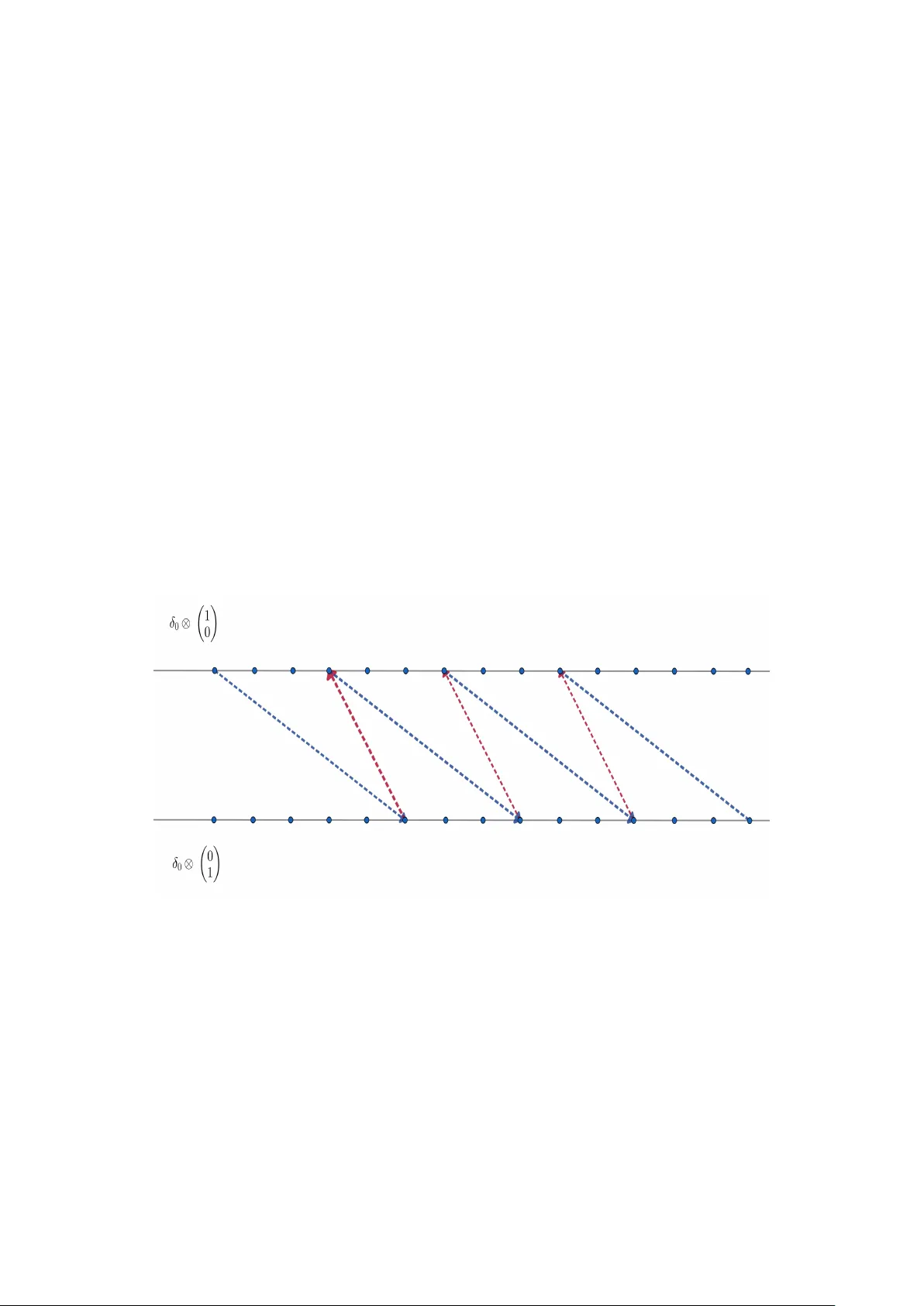
ER GODICITY IN DISCRETE-TIME QUANTUM W ALKS KIRAN KUMAR AND MOST AF A SABRI Abstract. W e undertak e a detailed analysis of ergo dicit y for homogeneous discrete- time quan tum walks on the in teger lattice. The most signiﬁcan t result of our paper holds in dimension one, and gives a complete equiv alence b etw een the absolutely con tinuous sp ectrum of the unitary operator enco ding the walk, and the equidistribution of its dynamics in position space, whic h app ears for the ﬁrst time in the context of large- v olume quantum ergo dicity . In higher dimensions, we give a criterion for full and partial ergo dicity in terms of a ﬁner prop erty of the sp ectrum which we dub “No Rep eating Graphs”, and distinguish how strongly the equidistribution is taking place (w eak con vergence vs total v ariation). The paper includes a w ealth of examples where w e apply our criteria, with certain families of walks fully characterized. Contents 1. In tro duction 1 2. Pro of of the general criterion 8 3. Fine analysis in dimension one 15 4. F ocus on t w o-state quan tum walks on the line 29 5. Higher dimensional walks 38 App endix A. Notations and mo dels in the literature 45 App endix B. RAGE theorem for quan tum walks 48 References 49 1. Introduction In this pap er we consider homogeneous quantum w alks ov er Z d with a ﬁnite n umber of spins. W e prov e that under the action of the w alk, lo calized initial states tend to equidistribute ov er the lattice as time grows large, provided certain sp ectral assumptions are met. This is illustrated by sev eral examples and non-examples. Our treatmen t is esp ecially complete in one dimension, where w e iden tify all semiclassical measures by a careful analysis and prov e a complete equiv alence b et w een the absolutely con tinuous sp ectrum and a form of ergodicity in p osition space. Let us giv e some bac kground. The problem of equidistribution of the quan tum dynamics on large graphs is v ery activ e and has an interesting history . Some of the earliest pap ers on quantum walks already considered this question [3, 33, 6]. In these pap ers, one starts with an initial state ψ of compact supp ort (e.g. a qubit), considers a unitary op erator U enco ding the walk, and studies whether the vector U k ψ b ecomes equidistributed in space as time go es on. T ec hnically , it is necessary to consider the time-av eraged evolution when w orking on a ﬁnite graph, otherwise the distribution will not con v erge [3]. In more detail, given a w alk with ν spins on a ﬁnite graph G , denote ∥ ϕ ( r ) ∥ 2 C ν = P ν i =1 | ϕ i ( r ) | 2 for r ∈ G and consider µ G T ,ψ ( r ) = 1 T P T − 1 k =0 ∥ ( U k ψ )( r ) ∥ 2 C ν . If the initial state ψ 2010 Mathematics Subje ct Classiﬁc ation. Primary 58J51. Secondary 47B93. Key wor ds and phr ases. Quan tum ergo dicit y , quan tum w alks, quan tum dynamics, absolutely con tin uous sp ectrum, delo calization. 1 2 KIRAN KUMAR AND MOST AF A SABRI is normalized, µ G T ,ψ ( r ) giv es (an a v eraged) probabilit y that the w alk is at position r at time T . It is easy to see that this quan tity con v erges as T → ∞ to µ G ψ ( r ) = P i ≤ m ∥ ( P λ i ψ )( r ) ∥ 2 C ν , where P λ i are the orthogonal pro jections onto the m distinct eigen v alues of U (for this simply write U k ψ = P i λ k i P λ i ψ and expand the square norm, noting that | λ i | = 1, the diagonal con tribution is µ G ψ ( r ), the oﬀ-diagonal part v anishes in the limit as a geometric sum divided by T ). The question is then whether µ G ψ is the uniform measure ov er G . This measure is diﬃcult to analyze unless the walk is very simple, as one needs to understand the structure of P k , whic h is generally problematic for large graphs. The pap er [3] sho ws that µ G ψ is uniform on G if G is the Cayley graph of an abelian group and if all eigen v alues of U are distinct. The eigenv alue assumption is restrictive, in fact the result is only applied to Hadamard w alks on odd cycles in [3]. The paper [6] later sho wed that µ G ψ is not uniform on even cycles. The discrepancy b etw een µ G ψ and the uniform measure v anishes how ever as the size of the cycle goes to inﬁnity . See Remark 4.4 for further discussion on this part icular w alk. This framew ork where the size of the graph grows large has b een explored in m uch greater generalit y in the realm of quantum chaos. In that context, giv en a sequence of graphs G N of size N , one lo oks instead at the orthonormal eigenv ectors ( ψ ( N ) j ) of the adjacency matrix of G N , and studies the limiting b ehaviour of the probability density | ψ ( N ) j ( v ) | 2 . Quan tum ergo dicit y is the statement that this densit y equidistributes when N → ∞ , for most eigenv ectors corresp onding to a sp ectral interv al I . The general picture established in [4, 12, 5, 32, 8] is that this should hold for an y orthonormal basis ( ψ ( N ) j ) of eigenfunctions, pro vided the graphs G N con v erge to some inﬁnite graph which has a “strong form” of absolutely contin uous spectrum. One also needs some tec hnical assumptions on G N for this. The pap ers [31, 34, 13] take a diﬀerent point of view, wherein there is no need to look at the limiting graph (if it exists), but only certain orthonormal bases ( ψ ( N ) j ) can b e con trolled. Bac k to quan tum w alks, it was sho wn in [10, 11] that qubits on G N b ecome uniformly spread out under the action of e − i tA G N , as the time t and size N grow large. This op erator is kno wn as the c ontinuous-time quantum walk on G N . As before, a time-av erage is actually necessary for this. The graphs G N considered in [10, 11] were graphs con v erging to a general Z d -p erio dic graph (crystal), for example the hexagonal lattice, strips and cylindrical hypercub es. In this pap er w e in vestigate ergo dicit y for homogeneous discr ete-time quantum walks on Z d . These are enco ded by iterations of a unitary op erator U which is not a priori asso ciated to any nice Schr¨ odinger op erator on G N . Suc h w alks are closer analogs to classical random walks. The Hilb ert space is H = ℓ 2 ( Z d ) ⊗ C ν , representing motion along Z d with ν p ossible spins. W e ﬁrst prov e a general criterion whic h says that if the op erator U on H has “nice” Flo quet eigenv alues, then the walk restricted to cubes G N con v erging to Z d , with perio dic b oundary conditions, is ergodic. In particular, if µ N T ,ψ ( r ) = 1 T P T − 1 k =0 ∥ ( U k N ψ )( r ) ∥ 2 C ν with ψ of compact supp ort and ∥ ψ ∥ = 1, and if µ N ψ ( r ) = lim T →∞ µ N T ,ψ ( r ), then µ N ψ approac hes the uniform measure µ N ( r ) = 1 N d on G N , as N → ∞ . “Nice” Flo quet eigenv alues should not b e ﬂat (we assume absolutely contin uous sp ectrum) and should not hav e a “high frequency” (no part of the graph of the eigenv alue, as a function of the quasimomen tum, should rep eat itself on sets of positive measure). Despite its generality , this abstract criterion is not the main purp ose of this pap er. T echnically sp eaking, its pro of is quite similar to the case of contin uous-time quan tum w alks previously established in [10]. Our main purp ose here is to inv estigate how far ERGODICITY IN DISCRETE-TIME QUANTUM W ALKS 3 this criterion applies to concrete quan tum w alks considered in the literature, illustrating examples and non-examples, and to see ho w far it can b e impro v ed. The strongest results w e obtain are in one dimension, where we establish for the ﬁrst time a complete equiv alence b et ween the absolutely contin uous sp ectrum of U (without an y additional assumptions on the Flo quet eigen v alues or resolven t) and the ergo dicity of U N in p osition space. This is obtained as a consequence of analyzing all semiclassical limits of µ N T ,ψ that arise when testing against a broader (nonregular) family of observ ables. 1.1. Mo del and deﬁnitions. W e consider a quan tum walk U on Z d with ν degrees of freedom (i.e. ν spins). The Hilbert space is th us H = ℓ 2 ( Z d ) ⊗ C ν , which we identify with ℓ 2 ( Z d ) ν = ℓ 2 ( Z d , C ν ). T o deﬁne U , let us ﬁrst in tro duce the shift operators S p : ℓ 2 ( Z d ) → ℓ 2 ( Z d ) δ k 7→ δ k + p where w e use boldface indices for p oints in Z d , R d . Our quantum walk U on ℓ 2 ( Z d , C ν ) acts on vector functions ψ =  ψ 1 · · · ψ ν  T with ψ j ∈ ℓ 2 ( Z d ) and is deﬁned b y (1.1) U =    U 1 , 1 U 1 , 2 · · · U 1 ,ν . . . . . . . . . U ν, 1 · · · U ν,ν    where U is unitary and each U i,j an op erator on ℓ 2 ( Z d ). W e assume the walk is homogeneous and of ﬁnite range, i.e. evolv es at a ﬁnite distance at eac h step. F or coined w alks, homogeneity means that the coin is independent of the p osition. More generally , our assumptions mean that there exists a ﬁnite set F ⊂ Z d and U i,j ( p ) ∈ C suc h that (1.2) U i,j = X p ∈ F U i,j ( p ) S p . If ψ ∈ ℓ 2 ( Z d , C ν ) is an initial state, its subsequen t time evolution is giv en b y U n ψ . In bra-ket notation, the w alk acts on a basis elemen t | j, k ⟩ ∈ C ν ⊗ ℓ 2 ( Z d ) by U : | j, k ⟩ 7→ ν X i =1 X p ∈ F U i,j ( p ) | i, k + p ⟩ . This means that a qubit at p osition k and spin j is mapped to a sup erp osition of states at p ositions k + p and spins i . W e do not use this notation m uch in the article, how ev er w e include a detailed translation in App endix A for readers who prefer it. Simple examples of w alks of the form (1.1)-(1.2) are the Hadamard and Gro v er w alks on Z are given b y the op erators (1.3) U Had = 1 √ 2  S − 1 S − 1 S 1 − S 1  and U Gro = 1 3   − S − 1 2 S − 1 2 S − 1 2 − 1 2 2 S 1 2 S 1 − S 1   i.e. each U i,j reduces to a single shift. See App endix A for the more common shift-coin deﬁnition, whic h is equiv alent to (1.3). Our framework is a lot more general and includes homogeneous split-step quantum walks, the shunt de c omp osition mo del , the ar c r eversal mo del , the higher dimensional PUTO mo del and more, see App endix A for details. 4 KIRAN KUMAR AND MOST AF A SABRI The op erator U : H → H given in (1.1)-(1.2) is unitarily equiv alen t to the op erator M b U on L 2 ( T d ) ν of multiplication b y the unitary Flo quet matrix function b U ( − θ ), where (1.4) b U ( θ ) =    b U 1 , 1 ( θ ) · · · b U 1 ,ν ( θ ) . . . b U ν, 1 ( θ ) · · · b U ν,ν ( θ )    and b U i,j ( θ ) = X p ∈ F U i,j ( p )e − 2 π i θ · p . Here T d ≡ [0 , 1) d . This result is kno wn; see Lemma 2.1 and the comment thereafter. Our conv en tion to take e − 2 π i θ · p rather than e 2 π i θ · p in b U ( θ ) is just to simplify notations that will arise later. W e ma y no w in troduce our results. Let L d N := { 0 , 1 , . . . , N − 1 } d ⊂ Z d b e a large b ox and let U N b e the restriction of U to ℓ 2 ( L d N , C ν ) with p erio dic boundary conditions. W e ﬁx an initial state ψ ∈ ℓ 2 ( L d N ) ν of compact supp ort (for example a qubit δ k ⊗ f ) and follow its evolution under U N . Assume ∥ ψ ∥ = 1. As in [3, 6, 27], w e deﬁne the probability that the quantum w alk on L d N , at time k , is at lo cation r , b y P N ( X k = r ) = ∥ ( U k N ψ )( r ) ∥ 2 C ν = ν X i =1 | [ U k N ψ ] i ( r ) | 2 and consider the time-av erage µ N T ,ψ ( r ) = 1 T T − 1 X k =0 P N ( X k = r ) = 1 T T − 1 X k =0 ν X i =1 | [ U k N ψ ] i ( r ) | 2 . This µ N T ,ψ is a probabilit y measure on L d N as µ N T ,ψ ( L d N ) = 1 T P T k =1 ∥ U k N ψ ∥ 2 = ∥ ψ ∥ 2 = 1, as U N is unitary . At time T = 0, µ N 0 ,ψ = ψ is fully lo c alized (think of ψ as a qubit). Our aim is to sho w that under some assumptions of sp ectral delo calization, µ N T ,ψ approac hes the uniform measure on L d N as T and N get large. This will b e done by comparing the a v erage of a function ϕ on L d N with resp ect to µ N T ,ψ and the uniform measure. The choice of these observ ables is imp ortant, so let us in tro duce the follo wing deﬁnition. Deﬁnition 1.1. W e sa y that ϕ ( N ) ∈ ℓ 2 ( L d N ) is a r e gular observable if it satisﬁes one of the following conditions: (i) ϕ ( N ) ( k ) = f ( k / N ) for some ﬁxed f ∈ H s ( T d ), with s > d/ 2, (ii) or ϕ ( N ) is the restriction to L d N of a summable function ϕ ∈ ℓ 1 ( Z d ). Recall that by the Sob olev embedding theorem, under assumption (i), f can be chosen to b e contin uous, and w e are implicitly making this c hoice here. Similarly , we say that a ∈ ℓ 2 ( L d N , C ν ) is a r e gular observable if eac h co ordinate a j ∈ ℓ 2 ( L d N ) is regular. Our strongest ergo dicit y results will hold if the follo wing sp ectral prop erty is satisﬁed : Deﬁnition 1.2. Let b U ( θ ) be the Flo quet matrix (1.4) with eigen v alues { E s ( θ ) } ν s =1 . W e sa y that the Flo quet eigenv alues ha v e No R ep e ating Gr aphs if ( NR G ) sup m  = 0 # { r ∈ L d N : E s ( r + m N ) − E w ( r N ) = 0 } N d − → 0 ∀ s, w ≤ ν as N → ∞ . ( NR G ) also stands for e n e rg y , as it is an assumption on the energies of b U ( θ ). Condition ( NR G ) app eared before in [32, 10] in the con text of ergodicity of eigen bases and contin uous-time quan tum walks. It implies that the sp ectrum of U is absolutely con tin uous with no eigen v alues, as U has an eigen v alue iﬀ E s ( θ ) = λ 0 is constan t [40], in which case E s ( r + m N ) = E s ( r N ) ∀ r , m and ( NR G ) is violated. F or quantum w alks on ERGODICITY IN DISCRETE-TIME QUANTUM W ALKS 5 Z , we prov e in Lemma 3.4 that ( NRG ) fails iﬀ E s ( θ + φ ) ≡ E w ( θ ) for some rational 0 < φ < 1. If s = w , this means that E s has a short perio d (high frequency). F or higher- dimensional walks, ( NR G ) seems to b e equiv alen t to the following statemen t: for any non-zero α ∈ [0 , 1) d ∩ Q d , the zero set of E s ( θ + α ) − E w ( θ ) has Lebesgue measure zero, see Remark 3.5. Note that having a Flo quet eigenv alue of higher multiplicit y , E s ( θ ) ≡ E w ( θ ), do es not violate ( NRG ). F or example, the walk  S 1 0 0 S 1  with Flo quet eigen v alues E 1 ( θ ) = E 2 ( θ ) = e − 2 π i θ satisﬁes ( NR G ). 1.2. Main results. Our ﬁrst result is the follo wing criterion for ergodicity . Theorem 1.3. L et U b e a quantum walk (1.1) - (1.2) satisfying ( NR G ) . L et ψ = P k ∈ Λ ψ ( k ) δ k b e an initial state of c omp act supp ort, i.e. Λ ⊂ Z d is ﬁnite and indep endent of N , and assume ∥ ψ ∥ = 1 . Then for any r e gular observable ϕ = ϕ ( N ) ∈ ℓ 2 ( L d N ) , ( PQE ) lim N →∞    lim T →∞ ⟨ ϕ ⟩ T ,ψ − ⟨ ϕ ⟩    = 0 , wher e ⟨ ϕ ⟩ T ,ψ = P r ∈ L d N ϕ ( r ) µ N T ,ψ ( r ) , while ⟨ ϕ ⟩ = 1 N d P r ∈ L d N ϕ ( r ) is the uniform aver age. Here ( PQE ) stands for p osition quantum er go dicity . Theorem 1.3 is a direct consequence of Theorem 1.7, whic h will yield a more precise ful l quantum er go dicity ( F QE ) in b oth p osition and spin spaces. Before we in tro duce it, let us explain ( PQE ) further. Theorem 1.3 shows that µ N T ,ψ ( r ) ≈ 1 N d in the sense of measures on L d N . As the space c hanges with N , w e cannot directly formulate this as a w eak. This can b e someho w ﬁxed. First recall that quite trivially , for ﬁxed N and any r ∈ L d N , (1.5) µ N T ,ψ ( r ) T →∞ − − − − → µ N ψ ( r ) , where µ N ψ ( r ) = P i ≤ m ∥ ( P λ ( N ) i ψ )( r ) ∥ 2 C ν (see the in tro duction). This is equiv alent to the w eak conv ergence µ N T ,ψ w − → µ N ψ . No w recall that we are considering p erio dic b oundary conditions, so in one dimension this amoun ts to studying the walk on a large cycle. T o ﬁx the space, w e may embed this cycle in to the unit circle. More generally , w e may deﬁne the measure e µ N T ,ψ on the torus T d b y e µ N ψ := X k ∈ L d N µ N ψ ( k ) δ k N so that e µ N ψ is concen trated on the set { k N : k ∈ L d N } , with e µ N ψ ( k N ) = µ N ψ ( k ). So w e deduce the following. Prop osition 1.4. L et ψ = P k ∈ Λ ψ ( k ) δ k b e an initial state of ﬁnite supp ort indep endent of N , and assume ∥ ψ ∥ = 1 . Then ( PQE ) for r e gular observables implies the we ak c onver genc e (1.6) e µ N ψ w − → µ wher e d µ ( x ) = d x is the uniform me asur e on T d . In p articular, (1.6) holds for any quantum walk (1.1) - (1.2) satisfying ( NR G ) . Recall that assumption ( NR G ) implies that U has no ﬂat bands, i.e. U has no eigen v alue. It is natural to exclude ﬂat bands. In fact, Prop osition 1.5. If U has a ﬂat b and, ther e exists some initial state ψ of c omp act supp ort, and a r e gular observable ϕ = ϕ N , such that ⟨ ϕ ⟩ T ,ψ = 1 and ⟨ ϕ ⟩ = c N d for al l T and N . In p articular, ( PQE ) fails. 6 KIRAN KUMAR AND MOST AF A SABRI In sp eciﬁc examples, w e can tak e the initial state ψ to b e a qubit. Lemma 1.6. The Gr over walk violates ( PQE ) for the initial state ψ = δ 0 ⊗ f and some observable ϕ , for any f = ( α, β , γ ) ∈ C 3 , ∥ f ∥ = 1 , such that f / ∈ span( 1 √ 6 , − 2 √ 6 , 1 √ 6 ) . Let us now discuss full ergo dicity: Theorem 1.7. L et U b e a quantum walk (1.1) - (1.2) satisfying ( NR G ) . Supp ose the observable a = a ( N ) ∈ ℓ 2 ( L d N ) ν is r e gular. Then for any initial state ψ of c omp act supp ort, ( F QE ) lim N →∞    lim T →∞ 1 T T X k =1 ⟨ U k N ψ , aU k N ψ ⟩ − ⟨ a ⟩ ψ    = 0 , wher e, denoting ⟨ a j ⟩ := 1 N d P k ∈ L d N a j ( k ) and P E s ( θ ) the sp e ctr al pr oje ctions c orr esp onding to the ν ′ ≤ ν distinct eigenvalues E s ( θ ) of b U ( θ ) , (1.7) ⟨ a ⟩ ψ = ν X j =1 ⟨ a j ⟩ X r ∈ L d N ν ′ X s =1    h P E s  r N  b ψ ( r ) i j    2 . This theorem is more precise than Theorem 1.3 b ecause it sho ws how the mass spreads out b oth in p osition space L d N and in spin space C ν . This spreading is ge nerally not uniform in spin space. The reason that we get the uniform measure in Theorem 1.3 is that w e sum ov er the spin con tributions to assess the probabilit y of b eing at some p osition r ∈ L d N . Still, the presence of ⟨ a j ⟩ implies uniformity in p osition space. T o make this more precise, we ma y em b ed the walk in the torus as b efore b y deﬁning e µ N ψ ,j = X k ∈ L d N µ N ψ ,j ( k ) δ k N where µ N ψ ,j ( r ) = lim T →∞ µ N T ,ψ ,j ( r ) and µ N T ,ψ ,j ( r ) = 1 T P T − 1 k =0 | [ U k N ψ ] j ( r ) | 2 . Then we ha v e Prop osition 1.8. L et ψ = P k ∈ Λ ψ ( k ) δ k b e an initial state of ﬁnite supp ort Λ ⊂ Z d indep endent of N , and assume ∥ ψ ∥ = 1 . Then ( FQE ) for r e gular observables implies the we ak c onver genc e (1.8) e µ N ψ ,j w − → c ψ ,j µ wher e d µ ( x ) = d x is the uniform me asur e on T d and c j,ψ is the explicit c onstant c ψ ,j = Z T d ν ′ X s =1     X m ∈ Λ [ P E s ( θ ) ψ ( m )] j e − 2 π i m · θ     2 d θ . In p articular, (1.8) holds for any quantum walk (1.1) - (1.2) satisfying ( NR G ) . In the sp ecial case where the initial state ψ = δ 0 ⊗ δ ℓ is a qubit with spin ℓ , w e get c j,ψ = R T d P ν ′ s =1 | P E s ( θ )( j, ℓ ) | 2 d θ . So far we show ed that for general quantum walks (1.1)-(1.2), ( NR G ) = ⇒ ( FQE ) = ⇒ ( PQE ) for regular observ ables. W e now specialize to d = 1 and study homogeneous ﬁnite- range quantum w alks o v er Z of ﬁnite range, where w e push the machinery to the limit and obtain a lot more precise results summarized in the following. Theorem 1.9 (One-dimensional walks) . L et U b e a quantum walk (1.1) - (1.2) over Z with an initial state ψ of c omp act supp ort, ∥ ψ ∥ = 1 . (1) If ( NRG ) holds, then ( FQE ) holds for al l observables a = a ( N ) with ∥ a ( N ) ∥ ∞ ≤ 1 . (2) If U has no ﬂat b ands, then ther e is always a subse quenc e N n such that ( NRG ) holds on L N n and ( F QE ) holds for al l a ( N n ) , ∥ a ( N n ) ∥ ∞ ≤ 1 . ERGODICITY IN DISCRETE-TIME QUANTUM W ALKS 7 (3) ( NRG ) fails iﬀ lim sup N sup m  =0 # { r ∈ L N : E s ( r + m N ) − E w ( r N ) } = ∞ . (4) If U has no ﬂat b ands, ( PQE ) c an fail for observables ϕ ( N ) with ∥ ϕ ( N ) ∥ ∞ ≤ 1 . Stil l, we ﬁnd al l “semiclassic al me asur es” in this c ase, and exhibit a phenomenon of e quidistribution on subsets (5) U has no ﬂat b ands iﬀ ( PQE ) holds for r e gular observables, for the ful l se quenc e. (6) Coine d walks U = S C with a 2 × 2 c oin and shifts to the right and left by distanc es α, β ∈ N ∗ exhibit al l kinds of dynamic al b ehaviors, and we ful ly char acterize them in terms of C , α and β . Split-step walks ar e also tr e ate d. (7) Ther e exist walks satisfying ( PQE ) for r e gular observables, but not for arbitr ary ∥ ϕ ( N ) ∥ ∞ ≤ 1 . Ther e exist walks satisfying ( PQE ) for ∥ ϕ ( N ) ∥ ∞ ≤ 1 , but not ( F QE ) for arbitr ary ∥ a ( N ) ∥ ∞ ≤ 1 . In (1),(2), we can actually tak e observ ables a ( N ) with sup norm gro wing not to o fast. W e summarize most of these ﬁndings in Figure 1. NR G F QE for b ounded obs. PQE for b ounded obs. PQE for regular obs. Absolutely con tinuous sp ectrum No ﬂat bands NR G on a subsequence × × Figure 1. Summary of results for w alks on Z . P articularly imp ortant is the equiv alence b etw een absolutely con tinuous spectrum and ergo dicit y of quan tum dynamics in position space for regular observ ables, which, to our kno wledge, app ears for the ﬁrst time in the literature on large-graph quantum c haos. This is obtained after a detailed analysis of the semiclassical measures in that con text. The equiv alence betw een absolutely con tin uous spectrum and the absence of ﬂat bands (eigen v alues) is classical on the other hand, as singularly con tin uous spectrum cannot exist in perio dic settings of ﬁnite range, see e.g. [40]. The fact that NR G on a subsequence implies absolutely contin uous sp ectrum is also immediate; as we said previously the presence of a ﬂat band w ould lead to E s ( r + m N n ) = E s ( r N n ) ∀ r , m . T o better appreciate the relev ance of assessing the ergo dicity of walks using b ounded observ ables, let us state the follo wing. Prop osition 1.10 (Conv ergence in total v ariation) . F or walks (1.1) - (1.2) on Z d , ( PQE ) holds for al l observables ∥ ϕ ( N ) ∥ ∞ ≤ 1 if and only if δ ( µ N ψ , µ N ) → 0 , wher e δ is the total variation distanc e and µ N ( r ) = 1 N d is the uniform me asur e on L d N . Similarly, ( F QE ) holds for al l observables a = a ( N ) with ∥ a ( N ) ∥ ∞ ≤ 1 if and only if δ ( µ N ψ ,j , c N ,ψ ,j µ N ) → 0 , wher e c N ,ψ ,j µ N is a c onstant multiple of µ N . One may naturally ask if results like Theorem 1.9 and Figure 1 hold in higher dimensions. Quite interestingly , we sho w that certain implications fail: 8 KIRAN KUMAR AND MOST AF A SABRI Prop osition 1.11. Ther e exists a quantum walk (1.1) - (1.2) over Z 2 which has pur ely absolutely c ontinuous sp e ctrum, but has no subse quenc e satisfying ( NRG ) . The same walk also violates ( PQE ) for r e gular observables. Finally , our results in one dimension also ha ve interesting applications for contin uous- time quan tum w alks and eigen v ectors ergo dicit y of p erio dic Sc hr¨ odinger op erators. W e collect these in § 3.4 to a v oid o v ercrowding the presen t section. 1.3. Op en questions. In view of Figure 1 and Prop osition 1.11, only the following questions remain op en: (1) Do es ( F QE ) for all observ ables a = a ( N ) with ∥ a ( N ) ∥ ∞ ≤ 1 imply ( NR G ) ? (2) In dimension d > 1, does ( NR G ) imply ( F QE ) for all observ ables a = a ( N ) with ∥ a ( N ) ∥ ∞ ≤ 1 ? There is also in terest in exploring ergo dicity beyond the presen t homogeneous setting. In particular, w alks on Z with non-constant perio dic coins, or with p erio dic electric ﬁelds [1, 2] are physically in teresting. W e exp ect a general criterion lik e Theorem 1.7 to hold in such p erio dic frameworks, how ev er in Theorem 1.3, one do es not exp ect µ N T ,ψ to b e p erfectly uniform an ymore, as its proﬁle will be aﬀected by the ﬁeld or the structure of the graph, if one goes b eyond Z d and studies general crystals. 1.4. Organization of the paper. W e start b y pro ving our general criteria in Section 2, namely the implications of ( NRG ) on ergodicity in general dimension, the implications on w eak conv ergence and conv ergence in total v ariation distance, and the fact that ﬂat bands preclude ( PQE ). In the follo wing Section 3, we sp ecialize to dimension one and prov e most of the results collected as Theorem 1.9. This is, in our view, the most important con tribution of the pap er. Section 4 specializes further to coined and split-step w alks, as they are quite popular mo dels in the literature, and w e bring some generalizations to these mo dels, where w e pla y with the step sizes of the walks and notice in teresting phenomena. In Section 5 w e explore v arious mo dels of quantum walks in higher dimension, some ergo dic, some not. In the case of the F ourier coin, we prov e ergo dicit y by combining our criterion with the irreducibility theory of Blo c h v arieties. Finally , in App endix A w e review other notations used in the literature for the reader’s conv enience, and some bac kground on models studied here, while in App endix B, we adapt the RA GE theorem to our quan tum w alks. W e include this here for completeness, as a diﬀerent more basic criterion linking the sp ectrum and dynamics, which is signiﬁcan tly easier to prov e. Ac kno wledgmen ts. W e w armly thank Houssam Ab dul-Rahman, W encai Liu and Armin Rainer for interesting discussions and clariﬁcations on their resp ectiv e works. 2. Proof of the general criterion In this section, after some basic F ourier analysis in § 2.1, we prov e Theorem 1.7 in 4 steps in § 2.2– § 2.5, and show that it implies Theorem 1.3 as a sp ecial case in § 2.6. W e then prov e Propositions 1.4, 1.8, 1.10 and 1.5 in § 2.7 – 2.9. 2.1. Basic F ourier Analysis. Consider a cube L d N ⊂ Z d and restrict U with p erio dic b oundary conditions: S p δ k = δ k + p with k i + p i mo d N . The restricted operator is denoted b y U N . W e ha v e (2.1) 1 T T − 1 X k =0 ⟨ U k N ψ , aU k N ψ ⟩ = ⟨ ψ , A T ψ ⟩ = ν X i =1 X v ∈ L d N ψ i ( v )( A T ψ ) i ( v ) ERGODICITY IN DISCRETE-TIME QUANTUM W ALKS 9 for A T = 1 T P T − 1 k =0 U ∗ k N aU k N . Throughout the section, we focus on ﬁnding the asymptotics of ( A T ψ ) i ( v ) b y moving to F ourier space. The starting point is to expand the function ( A T ψ ) i ∈ ℓ 2 ( L d N ) as a F ourier series (2.2) ( A T ψ ) i ( v ) = X r ∈ L d N ( [ A T ψ ) i ( r ) e ( N ) r ( v ) with e ( N ) r ( v ) := 1 N d/ 2 e 2 π i r · v / N , the basis of ℓ 2 ( L d N ) with F ourier co eﬃcients b φ ( r ) = 1 N d/ 2 P k ∈ L d N e − 2 π i k · r / N φ ( k ). W e deﬁne F ⊗ id : ℓ 2 ( L d N ) ν → ℓ 2 ( L d N ) ν    ψ 1 . . . ψ ν    7→    c ψ 1 . . . c ψ ν    , It follows from direct computation that for φ, ψ ∈ ℓ 2 ( L d N ) ν (2.3) [ φ · ψ = 1 N d/ 2 b φ ∗ b ψ , where ∗ denotes conv olution of functions, b φ ∗ b ψ ( r ) = P m ∈ L d N b φ ( m ) b ψ ( r − m ). Lemma 2.1. The op er ator U N on ℓ 2 ( L d N ) ν is unitarily e quivalent to ⊕ r ∈ L d N b U  − r N  on ℓ 2 ( L d N ) ν , wher e b U ( θ ) is the matrix (1.4) . Pr o of. W e observe that for φ ∈ ℓ 2 ( L d N ) ν , U N ( F ⊗ id) φ =    P ν j =1 P p U 1 ,j ( p ) S p b φ j . . . P ν j =1 P p U ν,j ( p ) S p b φ j    and due to p erio dic b oundary conditions, (2.4) S p b φ j = S p X k ∈ L d N b φ j ( k ) δ k = X k ∈ L d N b φ j ( k ) δ k + p = X k ∈ L d N b φ j ( k − p ) δ k . Let ϵ p ( k ) = e 2 π i p · k / N = N d/ 2 e ( N ) p ( k ). Since b φ ( r − p ) = 1 N d/ 2 X k ∈ L d N e − 2 π i( r − p ) · k / N φ ( k ) = ( d ϵ p φ )( r ) , w e get S p b φ j = [ ϵ p φ j , and thus [( F − 1 ⊗ id) U N ( F ⊗ id) φ ]( r ) =    P j P p U 1 ,j ( p )e 2 π i r · p / N φ j ( r ) . . . P j P p U ν,j ( p )e 2 π i r · p / N φ j ( r )    = b U  − r N  φ ( r ) . □ The same pro of shows that the full op erator U on ℓ 2 ( Z d ) ν is unitarily equiv alen t to multiplication b y the matrix function b U ( − θ ) on L 2 ( T d ) ν . Here w e use the F ourier transform F ⊗ id : L 2 ( T d ) ⊗ C ν → ℓ 2 ( Z d ) ⊗ C ν , taking f ⊗ δ i 7→ b f ⊗ δ i , b f ( k ) = R T d e − 2 π i θ · k f ( θ )d θ , with in v erse ( a k ) ⊗ δ i 7→ a ⊗ δ i , a ( θ ) = P k a k e 2 π i k · θ . 10 KIRAN KUMAR AND MOST AF A SABRI F or example, for the Hadamard and Grov er w alks in (1.3), this gives b U Had ( θ ) = 1 √ 2  e 2 π i θ e 2 π i θ e − 2 π i θ − e − 2 π i θ  and b U Gro ( θ ) = 1 3   − e 2 π i θ 2e 2 π i θ 2e 2 π i θ 2 − 1 2 2e − 2 π i θ 2e − 2 π i θ − e − 2 π i θ   . 2.2. Step 1. F rom the Heisen b erg picture to a phase space op erator. Back to (2.1), given an observ able a ∈ ℓ 2 ( L d N ) ν , we need to ﬁnd for k ∈ N , ( U ∗ k N aU k N ψ )( r ) . Recall (1.1). W e hav e ( U k ) i,j = X j 1 ,j 2 ,...,j k − 1 U i,j 1 U j 1 ,j 2 · · · U j k − 1 ,j = X j 1 ,j 2 ,...,j k − 1 X p 1 , p 2 ,..., p k U i,j 1 ( p 1 ) U j 1 ,j 2 ( p 2 ) · · · U j k − 1 ,j ( p k ) S p 1 + p 2 + ··· + p k . In (2.2) we are in terested in F ourier co eﬃcients. Similarly to (2.4), d S p g ( r ) = X k g ( k ) [ S p δ k ( r ) = X k g ( k ) [ δ k + p ( r ) = X k g ( k ) e − 2 π i( k + p ) · r N N d/ 2 = e − 2 π i p · r N b g ( r ) Therefore, ( [ U k N ψ ) i ( r ) = ν X j =1 \ U k i,j ψ j ( r ) = ν X j =1 X j 1 ,...,j k − 1 X p 1 ,..., p k U i,j 1 ( p 1 ) U j 1 ,j 2 ( p 2 ) · · · U j k − 1 ,j ( p k )e − 2 π i r · ( p 1 + ··· + p k ) / N b ψ j ( r ) = ν X j =1 X j 1 ,...,j k − 1 b U  r N  i,j 1 b U  r N  j 1 ,j 2 · · · b U  r N  j k − 1 ,j b ψ j ( r ) = h b U  r N  k b ψ ( r ) i i . On the other hand, b y (2.3), \ ( aU k N ψ ) i ( r ) = 1 N d/ 2 [ b a ∗ [ U k N ψ ] i ( r ) = 1 N d/ 2 X m ∈ L d N b a i ( m )( [ U k N ψ ) i ( r − m ) = 1 N d/ 2 X m ∈ L d N b a i ( m ) h b U  r − m N  k b ψ ( r − m ) i i where r − m is tak en mod N . No w ( U ∗ ) i,j = P p U j,i ( p ) S − p and ( b U ( θ ) ∗ ) i,j = P p U j,i ( p )e 2 π i θ · p . So w e similarly get ( \ U ∗ k ψ ) i ( r ) = P j P j 1 ,...,j k − 1 P p 1 ,..., p k U j 1 ,i ( p 1 ) . . . U j,j k − 1 ( p k )e 2 π i r · ( p 1 + ··· + p k ) / N b ψ j ( r ) = ERGODICITY IN DISCRETE-TIME QUANTUM W ALKS 11 [ b U ( r N ) ∗ k b ψ ( r )] i . W e ma y th us expand as in (2.2) to get [ U ∗ k N aU k N ψ ] i ( v ) = X r ∈ L d N \ [ U ∗ k N aU k N ψ ] i ( r ) e ( N ) r ( v ) = X r ∈ L d N h b U  r N  ∗ k ( \ aU k N ψ )( r ) i i e ( N ) r ( v ) = X r ∈ L d N ν X j =1 b U  r N  ∗ k i,j \ ( aU k N ψ ) j ( r ) e ( N ) r ( v ) = 1 N d/ 2 X r ∈ L d N ν X j =1 b U  r N  ∗ k i,j X m ∈ L d N b a j ( m ) h b U  r − m N  k b ψ ( r − m ) i j e ( N ) r ( v ) = 1 N d/ 2 X r , m ∈ L d N ν X j,ℓ =1 b U  r N  ∗ k i,j b a j ( m ) b U  r − m N  k j,ℓ b ψ ℓ ( r − m ) e ( N ) r ( v ) . Let E 1 ( θ ) , . . . , E ν ′ ( θ ) denote the distinct eigen v alues of b U ( θ ), with resp ective eigenpro jections P E 1 ( θ ) , . . . P E ν ′ ( θ ). Note that ν ′ ma y dep end on θ , but this will not aﬀect the following calculations. W e denote ν ′ 1 = ν ′ ( r + m N ) and ν ′ 2 = ν ′ ( r N ). Since b U k ( θ ) = P ν ′ s =1 E s ( θ ) k P s ( θ ) and b U ( θ ) ∗ k = P ν ′ s =1 E s ( θ ) k P s ( θ ), we get that [ U ∗ k N aU k N ψ ] i ( v ) = 1 N d/ 2 X r , m ∈ L d N ν X j,ℓ =1 X s,t  E s  r N  E t  r − m N   k P E s  r N  ( i, j ) · b a j ( m ) P E t  r − m N  ( j, ℓ ) b ψ ℓ ( r − m ) e ( N ) r ( v ) = X r , m ∈ L d N ν X j,ℓ =1 ν ′ 1 X s =1 ν ′ 2 X t =1  E s  r + m N  E t  r N   k P E s  r + m N  ( i, j ) · b a j ( m ) P E t  r N  ( j, ℓ ) b ψ ℓ ( r ) e ( N ) r + m ( v ) N d/ 2 . Deﬁne F T ( v , r ; i, ℓ ) = X m ∈ L d N ν X j =1 ν ′ 1 X s =1 ν ′ 2 X t =1 1 T T − 1 X k =0  E s  r + m N  E t  r N   k · P E s  r + m N  ( i, j ) b a j ( m ) P E t  r N  ( j, ℓ ) e ( N ) m ( v ) , and (2.5) [Op N ( F ) ψ ] i ( v ) = X r ∈ L d N ν X ℓ =1 F ( v , r ; i, ℓ ) b ψ ℓ ( r ) e ( N ) r ( v ) Then using 1 N d/ 2 e ( N ) m + r = e ( N ) m e ( N ) r , we get 1 T T − 1 X k =0 [ U ∗ k N aU k N ψ ] i ( v ) = X r ∈ L d N ν X ℓ =1 F T ( v , r ; i, ℓ ) b ψ ℓ ( r ) e ( N ) r ( v ) = [Op N ( F T ) ψ ] i ( v ) , and so, our main quan tity (2.1) takes the form (2.6) 1 T T − 1 X k =0 ⟨ U k N ψ , aU k N ψ ⟩ = ν X i =1 X v ∈ L d N ψ i ( v )[Op N ( F T ) ψ ] i ( v ) = ⟨ ψ , Op N ( F T ) ψ ⟩ . 12 KIRAN KUMAR AND MOST AF A SABRI 2.3. Step 2. The time limit in a ﬁnite spacial b o x. Lemma 2.2. F or any ﬁxe d N , we have lim T →∞ ⟨ ψ , Op N ( F T ) ψ ⟩ = ⟨ ψ , Op N ( b ) ψ ⟩ for b ( v , r , i, ℓ ) = X m ∈ L d N ν X j =1 ν ′ 1 X s =1 ν ′ 2 X t =1 1 S r ( m , s, t ) P E s  r + m N  ( i, j ) b a j ( m ) P E t  r N  ( j, ℓ ) e ( N ) m ( v ) , and S r = { ( m , s, t ) : E s ( r + m N ) = E t ( r N ) } . Pr o of. Recalling (2.5), if ψ = P k ∈ Λ ψ ( k ) δ k has compact supp ort Λ ⊂ Z d indep enden t of N , then ⟨ ψ , Op N ( F ) ψ ⟩ = P ν i =1 P v ∈ Λ ψ i ( v ) P r ∈ L d N P ν ℓ =1 F ( v , r ; i, ℓ ) b ψ ℓ ( r ) e ( N ) r ( v ). Also, b ψ ℓ ( r ) = P k ′ ∈ Λ e ( N ) r ( k ′ ) ψ ℓ ( k ′ ). Thus, (2.7) |⟨ ψ , Op N ( F ) ψ ⟩| ≤ C Λ max i,ℓ, v , k ′    1 N d X r ∈ L d N F ( v , r ; i, ℓ )e 2 π i r · ( v − k ′ ) / N    . W e thus examine the diﬀerence of sym b ols. Let α s,t, r , m ,N = ( E s  r + m N  E t  r N  . If ( m , s, t ) ∈ S r , then 1 T P T − 1 k =0 α k s,t, r , m ,N = 1. Otherwise, the sum is geometric. Thus, |⟨ ψ , Op N ( F T − b ) ψ ⟩| ≤ C Λ max i,ℓ, v , k ′ 1 N d X r , m ∈ L d N ν X j =1 X s,t 1 S c r ( m , s, t ) ·    1 − α T s,t, r , m ,N T [1 − α s,t, r , m ,N ] P E s  r + m N  ( i, j ) b a j ( m ) P E t  r N  ( j, ℓ )    ≤ C N ,a T , where C N ,a is ﬁnite for any N and is indep endent of T . T aking T → ∞ yields the result. □ 2.4. Step 3. The zero order symbol yields a weigh ted av erage. W e deduce from (2.6) and Lemma 2.2 that (2.8) lim T →∞ 1 T T − 1 X k =0 ⟨ U k N ψ , aU k N ψ ⟩ = ⟨ ψ , Op N ( b ) ψ ⟩ = ⟨ ψ , Op N ( b 0 ) ψ ⟩ + ⟨ ψ , Op N ( b ′ ) ψ ⟩ , where b 0 is the contribution of m = 0 , i.e. b 0 ( v , r , i, ℓ ) = ν X j =1 ν ′ 2 X s,t =1 1 S r ( 0 , s, t ) P E s  r N  ( i, j ) b a j ( 0 ) P E t  r N  ( j, ℓ ) e ( N ) 0 ( v ) , b ′ ( v , r , i, ℓ ) = X m  = 0 ν X j =1 ν ′ 1 X s =1 ν ′ 2 X t =1 1 S r ( m , s, t ) P E s  r + m N  ( i, j ) b a j ( m ) P E t  r N  ( j, ℓ ) e ( N ) m ( v ) . Let ν ′ := ν ′ 2 . Since b a j ( 0 ) = 1 N d/ 2 P k ∈ L d N a j ( k ) = N d/ 2 ⟨ a j ⟩ and e ( N ) 0 ( v ) = N − d/ 2 , b 0 ( v , r , i, ℓ ) = ν X j =1 ν ′ X s,t =1 1 S r ( 0 , s, t ) P E s  r N  ( i, j ) ⟨ a j ⟩ P E t  r N  ( j, ℓ ) , ERGODICITY IN DISCRETE-TIME QUANTUM W ALKS 13 By deﬁnition (2.5), we get [Op N ( b 0 ) ψ ] i ( v ) = X r ∈ L d N ν X ℓ =1 ν ′ X s,t =1 E s ( r N )= E t ( r N ) ν X j =1 P E s  r N  ( i, j ) ⟨ a j ⟩ P E t  r N  ( j, ℓ ) b ψ ℓ ( r ) e ( N ) r ( v ) = ν X j =1 ⟨ a j ⟩ X r ∈ L d N ν X ℓ =1 ν ′ X s =1 P E s  r N  ( i, j ) P E s  r N  ( j, ℓ ) b ψ ℓ ( r ) e ( N ) r ( v ) = ν X j =1 ⟨ a j ⟩ X r ∈ L d N ν ′ X s =1 P E s  r N  ( i, j ) h P E s  r N  b ψ ( r ) i j e ( N ) r ( v ) . where ν ′ is the num ber of distinct eigen v alues of b U ( r N ). Thus, w e sho w ed that ⟨ ψ , Op N ( b 0 ) ψ ⟩ = ν X i,j =1 ⟨ a j ⟩ X r ∈ L d N ν ′ X s =1 X v ∈ L d N P E s  r N  ( j, i ) ψ i ( v ) e ( N ) r ( v ) h P E s  r N  b ψ ( r ) i j = ν X j =1 ⟨ a j ⟩ X r ∈ L d N ν ′ X s =1 h P E s  r N  b ψ ( r ) i j h P E s  r N  b ψ ( r ) i j = ⟨ a ⟩ ψ (2.9) as given in (1.7), where w e used that b f ( r ) = P v f ( v ) e ( N ) r ( v ). Remark 2.3. Observ e that in Steps 1-3 w e ha v e not used the regularity of the observ able, in particular, the previous results hold for an y a ( N ) with ∥ a ( N ) ∥ ∞ ≤ 1. 2.5. Step 4. The higher order mo des v ani sh asymptotically . W e no w sho w that Op N ( b ′ ) is asymptotically negligible. Recalling (2.7), taking F = b ′ , it suﬃces to sho w that the term in the modulus go es to zero. This term is 1 N d X r ∈ L d N X m  = 0 ν X j,s,w =1 1 S r ( m , s, w ) P s  r + m N  ( i, j ) b a j ( m ) P w  r N  ( j, ℓ ) e ( N ) m ( v )e 2 π i r · ( v − k ′ ) / N . Here, if ( u s ( θ ) , E s ( θ )) is an orthonormal eigensystem of b U ( θ ), then P s ( θ ) f = ⟨ f , u s ( θ ) ⟩ u s ( θ ). In other w ords, P E s = P P s , where the sum runs ov er the u s ( θ ) with eigen v alue E s ( θ ). Let A m = { ( r , s, w ) : E s ( r + m N ) − E w ( r N ) = 0 } . Then ( m , s, w ) ∈ S r ⇐ ⇒ ( r , s, w ) ∈ A m so the ab ov e is 1 N d X m  = 0 ν X j =1 b a j ( m ) e ( N ) m ( v ) X r ∈ L d N ν X s,w =1 1 A m ( r , s, w ) P s  r + m N  ( i, j ) P w  r N  ( j, ℓ )e 2 π i r · ( v − k ′ ) / N . W e will sho w that for regular a ( N ) , there is C a indep enden t of N suc h that (2.10) X m ν X j =1 | b a j ( m ) e ( N ) m ( v ) | ≤ C a . Since by ( NR G ), sup m  = 0 | A m | N d → 0, then using | P s ( θ )( i, j ) | ≤ 1, we will get ⟨ ψ , Op N ( b ′ ) ψ ⟩ → 0. In view of (2.8) and (2.9), this will complete the pro of. Let’s pro v e (2.10). If a j ( k ) = f j ( k / N ) with f j ∈ H s ( T d ), s > d/ 2, where ∥ f ∥ 2 H s = P k ∈ Z d | ˆ f ( k ) | 2 ⟨ k ⟩ 2 s , ˆ f ( k ) = R T d e − 2 π i k · x f ( x ) d x and ⟨ k ⟩ = p 1 + | k | 2 , then ∥ ˆ f ∥ 1 := P k | ˆ f ( k ) | ≤ C s ∥ f ∥ H s , where C 2 s = P k ⟨ k ⟩ − 2 s < ∞ since 2 s > d . On the other hand, f = P k ˆ f ( k ) e k with e k ( x ) = e 2 π i k · x , so b a j ( m ) = ⟨ e ( N ) m , f j ( · / N ) ⟩ ℓ 2 (Λ N ) = 14 KIRAN KUMAR AND MOST AF A SABRI P k ∈ Z d ˆ f j ( k ) ⟨ e ( N ) m , e k ( · / N ) ⟩ ℓ 2 (Λ N ) = ˆ f j ( m ) N d/ 2 , since e k ( n / N ) = N d/ 2 e ( N ) k ( n ). This implies P m P j | b a j ( m ) e ( N ) m ( v ) | ≤ P j ∥ ˆ f j ∥ 1 , which is ﬁnite. The second class of a ( N ) are the restrictions of a ∈ ℓ 1 ( Z d ) ν . Here, a j = P n ∈ Z d P ν q =1 c n ,j δ n with P n | c n ,j | < ∞ . Then b a j ( m ) = P n ∈ Z d c n ,j e ( N ) m ( n ). This implies | b a j ( m ) e ( N ) m ( v ) | ≤ 1 N d ∥ a ∥ 1 for all j implying (2.10). Com bining the steps together, w e ha v e ﬁnally completed the proof of Theorem 1.7. 2.6. F rom FQE to PQE. T ak e a ∈ ℓ 2 ( L d N ) ν suc h that a j = ϕ ∀ j . Then (1.7) becomes ⟨ a ⟩ ψ = ⟨ ϕ ⟩ X r ∈ L d N ν ′ X s =1    P E s  r N  b ψ ( r )    2 C ν = ⟨ ϕ ⟩ X r ∈ L d N ∥ b ψ ( r ) ∥ 2 C ν = ⟨ ϕ ⟩∥ b ψ ∥ 2 ℓ 2 ( L d N ) ν = ⟨ ϕ ⟩∥ ψ ∥ 2 = ⟨ ϕ ⟩ since ∥ ψ ∥ = 1. On the other hand, 1 T T − 1 X k =0 ⟨ U k N ψ , aU k N ψ ⟩ = 1 T T − 1 X k =0 ν X i =1 X r ∈ L d N a i ( r ) | [ U k N ψ ] i ( r ) | 2 = X r ∈ L d N ϕ ( r ) µ N T ,ψ ( r ) = ⟨ ϕ ⟩ T ,ψ . Th us, Theorem 1.7 implies Theorem 1.3. 2.7. F rom QE to weak conv ergence. Let a j = ϕ and a i = 0 for i  = j . Then 1 T P T − 1 k =0 ⟨ U k N ψ , aU k N ψ ⟩ = P m ∈ L d N ϕ ( m ) 1 T P T − 1 k =0 | [( U k N ψ )( m )] j | 2 → P m ∈ L d N ϕ ( m ) µ N ψ ,j ( m ) =: ⟨ ϕ ⟩ ψ ,j as T → ∞ . Th us, ( FQE ) implies that |⟨ ϕ ⟩ ψ ,j − ⟨ ϕ ⟩ c N ,ψ ,j | → 0 as N → ∞ , where c N ,ψ ,j := P r ∈ L d N P ν ′ s =1 | [ P E s ( r N ) b ψ ( r )] j | 2 . Note that b ψ ( r ) = 1 N d/ 2 P k ∈ Λ e − 2 π i k · r N ψ ( k ), where Λ is the compact support of ψ , which is indep endent of N . So by linearit y , h P E s  r N  b ψ ( r ) i j = 1 N d/ 2 X k ∈ Λ h P E s  r N  ψ ( k ) i j e − 2 π i k · r N . Hence, c N ,ψ ,j = 1 N d X r ∈ L d N ν ′ X s =1      X k ∈ Λ h P E s  r N  ψ ( k ) i j e − 2 π i k · r N      2 , This is a Riemann sum of a con tin uous function and therefore, c N ψ ,j N →∞ − − − − → Z T d ν ′ X s =1      X k ∈ Λ  P E s ( θ ) ψ ( k )  j e − 2 π i k · θ      2 d θ = c ψ ,j . No w take ϕ ( m ) = f ( m / N ) with f ∈ H s ( T d ) contin uous. Then ⟨ ϕ ⟩ → R T d f ( x ) d x . Thus, ( F QE ) implies that Z T d f ( x ) d e µ N ψ ,j ( x ) = ⟨ ϕ ⟩ ψ ,j − ⟨ ϕ ⟩ c N ,ψ ,j + ⟨ ϕ ⟩ c N ,ψ ,j → c ψ ,j Z T d f ( x ) d x for any contin uous f ∈ H s ( T d ), in particular, for an y smooth f . Combin ing [23, Cor 15.3, Thm 13.34], we deduce that e µ N ψ ,j w − → c ψ ,j µ as N → ∞ . This pro v es Proposition 1.8. The pro of of Prop osition 1.4 is the same, with simpler notations. ERGODICITY IN DISCRETE-TIME QUANTUM W ALKS 15 2.8. Con v ergence in total v ariation. W e turn to the proof of Prop osition 1.10. Recall that δ ( µ, µ ′ ) = 1 2 P x | µ ( x ) − µ ′ ( x ) | . Supp ose ( PQE ) holds for all observ ables ∥ ϕ ( N ) ∥ ∞ ≤ 1. This means that | P k ∈ L d N ϕ ( N ) ( k )( µ N ψ ( k ) − 1 N d ) | → 0. Cho osing ϕ ( N ) ( k ) = sgn( µ N ψ ( k ) − 1 N d ), this yields P k ∈ L d N | µ N ψ ( k ) − 1 N d | → 0, and th us δ ( µ N ψ , µ N ) → 0. Con v ersely , if δ ( µ N ψ , µ N ) → 0, then by the triangle inequality , | P k ϕ ( N ) ( k )( µ N ψ ( k ) − 1 N d ) | ≤ 2 δ ( µ ( N ) ψ , µ ) → 0. 2.9. Compact supp ort of eigenv ectors. W e next prov e Prop osition 1.5 and Lemma 1.6. W e start with the follo wing result. Lemma 2.4. If the ful l quantum walk op er ator U in (1.1) - (1.2) has an eigenvalue λ 0 , i.e. a ﬂat b and, then ther e exists a c orr esp onding eigenve ctor for λ 0 of c omp act supp ort. Pr o of. If U has a ﬂat band λ 0 , then its Flo quet matrix (1.4) has a corresp onding eigen v ector f ( θ ), with b U ( θ ) f ( θ ) = λ 0 f ( θ ) for all θ [40]. Since U is of ﬁnite range, eac h entry of b U ( θ ) is a trigonometric p olynomial. The same pro of as [37, Lemma 2.5] sho ws that w e can c ho ose f ( θ ) to b e a trigonometric p olynomial in each en try , say f p ( θ ) = P m ∈ Λ p α p ( m )e 2 π i m · θ . On the other hand, b U = ( F − 1 ⊗ id) U ( F ⊗ id). Thus, U ( F ⊗ id) f = λ 0 ( F ⊗ id) f , so ( F ⊗ id) f =    b f 1 . . . b f ν    is an eigenv ector of U . Here, b f ( k ) = R T d e − 2 π i θ · k f ( θ )d θ . So w e get b f p ( k ) = α p ( k ) if k ∈ Λ p and 0 otherwise. Th us, ( F ⊗ id) f is an eigenv ector of U of compact supp ort. □ Pr o of of Pr op osition 1.5. By Lemma 2.4, if U has a ﬂat band, then U has a corresp onding eigen v ector ψ of compact supp ort. Sa y as a v ector, ψ ( k ) = 0 if k / ∈ Λ. W e normalize ∥ ψ ∥ = 1. T aking N big enough, we hav e Λ ⊂ L d N and U N ψ = U ψ = λ 0 ψ . Hence, µ N T ,ψ ( r ) = 1 T P T − 1 k =0 P ν i =1 | ( U k N ψ ) i ( r ) | 2 = 1 T P T − 1 k =0 P ν i =1 | ψ i ( r ) | 2 = ∥ ψ ( r ) ∥ 2 C ν , since | λ 0 | = 1. Cho ose ϕ = ϕ ( N ) ≡ 1 on Λ and ϕ = 0 on L d N \ Λ. Then ⟨ ϕ ⟩ T ,ψ = P r ϕ ( r ) µ N T ,ψ ( r ) = ∥ ψ ∥ 2 = 1. On the other hand, ⟨ ϕ ⟩ = | Λ | N d = c N d with c independent of N . Here ϕ is regular as it has a compact supp ort (so is in ℓ 1 ). □ Pr o of of L emma 1.6. Consider the initial state ψ = δ 0 ⊗ f , where f = ( α, β , γ ). It is sho wn in [19, Section 3] that lim N →∞ lim T →∞ 1 T 3 X l =1 T − 1 X t =0 P N (0 , t ; l ; α, β , γ ) = (5 − 2 √ 6)(1 + | α + β | 2 + | β + γ | 2 − 2 | β | 2 ) =: c α,β ,γ where P N (0 , t ; l ; α, β , γ ) is the probability of ﬁnding the particle with c hiralit y l at p osition 0 and time t on the cyclic lattice with N sites. In other words, 1 T P 3 l =1 P T − 1 t =0 P N (0 , t ; l ; α, β , γ ) = µ N T ,ψ (0). T ake the observ able ϕ = δ 0 on L N . Then ⟨ ϕ ⟩ T ,ψ = µ N T ,ψ (0) and ⟨ ϕ ⟩ = 1 N d . Thus, lim N →∞ | lim T →∞ ⟨ ϕ ⟩ T ,ψ − ⟨ ϕ ⟩| = c α,β ,γ > 0 if ( α, β , γ )  = ( 1 √ 6 , − 2 √ 6 , 1 √ 6 ) or a constant m ultiple of it. □ 3. Fine anal ysis in dimension one In this section we pro ve particularly strong ergo dicity results whic h hold for one- dimensional w alks, and were collectively stated in Theorem 1.9. W e start with (1)–(3). W e will often use the fact that in dimension one, the Flo quet eigenv alue functions are analytic in the full parameter space θ ∈ R , see [36, Proposition 5.3]. 16 KIRAN KUMAR AND MOST AF A SABRI Our ﬁrst statemen t is that in dimension one, ( NR G ) implies ( F QE ) not only for regular observ ables, but for bounded observ ables in general. Theorem 3.1. L et U b e a discr ete-time quantum walk on Z as in (1.1) - (1.2) . If U satisﬁes ( NR G ) , then it satisﬁes ( F QE ) for any observable a ( N ) such that ∥ a ( N ) ∥ ∞ ≤ 1 . Our second statement is that in the absence of ﬂat bands, there is alwa ys a subsequence satisfying ( NRG ), and o v er which w e ma y apply the conclusion of Theorem 3.1. Theorem 3.2. Consider a family of normal ν × ν matric es { b U ( θ ) } θ ∈ [0 , 1) with analytic entries. Supp ose b U ( θ ) do es not have a ﬂat b and. Then ( NRG ) holds on a subse quenc e. That is, ther e exists a strictly incr e asing se quenc e ( N n ) such that (3.1) sup m  =0 # { r ∈ L N n : E s ( r + m N n ) − E w ( r N n ) = 0 } N n → 0 for al l s, w . As a r esult, ( F QE ) holds along L N n for al l a ( N n ) such that ∥ a ( N n ) ∥ ∞ ≤ 1 . In Prop osition 5.7, we sho w that Theorem 3.2 is in general not true for higher- dimensional quantum w alks. T o pro v e the ab o v e theorems, w e state tw o lemmas. The proofs of these lemmas are pushed to Section 3.1. W e sa y a function E : Ω → C is p erio dic if ∃ α > 0 suc h that { θ : E ( θ + α )  = E ( θ ) } is a set of measure zero. F or an analytic function on a domain Ω, this is equiv alent to saying that E ( θ + α ) = E ( θ ) for all θ ∈ Ω. The smallest such α is called the perio d of E . Lemma 3.3. F or a non-c onstant analytic function E : R → C with a r ational p erio d α , deﬁne F ( θ ) := E ( θ + φ ) for al l θ and some ﬁxe d 0 < φ ≤ α . Then F ( θ ) = E ( θ + uα + φ ) for al l u ∈ Z . Mor e over, ther e exist se quenc es N n → ∞ , m n ∈ L N n and a c onstant c > 0 such that (3.2) # n r ∈ L N n : E  r + m n N n  − F  r N n  = 0 o ≥ cN n for al l but ﬁnitely many n if and only if for al l but ﬁnitely many n , m n N n is of the form φ + uα for some non-ne gative inte ger u < 1 α . In p articular, if α ≥ 1 , then m n N n = φ for al l but ﬁnitely many n . Lemma 3.4. Consider a family of ν × ν normal matric es { b U ( θ ) } θ ∈ R with analytic entries and eigenvalues E 1 ( θ ) , E 2 ( θ ) , . . . , E ν ( θ ) . Fix 1 ≤ s, w ≤ ν . Then the fol lowing ar e e quivalent (i) ( NRG ) fails for s and w : (3.3) sup m  =0 m ∈ L N # { r ∈ L N : E s ( r + m N ) − E w ( r N ) = 0 } N ↛ 0 . (ii) lim sup N →∞ sup m  =0 m ∈ L N # n r ∈ L N : E s  r + m N  − E w  r N  = 0 o = ∞ . (iii) Ther e exists a r ational 0 < φ < 1 such that E s ( θ + φ ) = E w ( θ ) for al l θ ∈ R . A dditional ly, if ther e exists a subse quenc e ( m n k ) such that the fr action in (3.3) do es not c onver ge to zer o and m n k N n k → 0 , then E s ( θ ) , E w ( θ ) ar e ﬂat b ands and E s ( θ ) ≡ E w ( θ ) ≡ c for some c ∈ C . No w we pro v e Theorems 3.1 and 3.2, assuming Lemmas 3.3 and 3.4. ERGODICITY IN DISCRETE-TIME QUANTUM W ALKS 17 Pr o of of The or em 3.1. As we men tioned in Remark 2.3, the only place in the pro of of Theorem 1.7 where we needed the observ able assumption is in Step 4 (Section 2.5). Therefore, to prov e the theorem, it is suﬃcient to sho w that for an y ∥ a ( N ) ∥ ∞ ≤ 1, (3.4) 1 N X m  =0 ν X j =1 b a j ( m ) e ( N ) m ( v ) X r ∈ L N ν X s,w =1 1 A m ( r , s, w ) P s  r + m N  ( i, j ) P w  r N  ( j, ℓ )e 2 π i r v − k ′ N go es to zero for all v , i, ℓ and k ′ , with A m := { ( r , s, w ) : E s ( r + m N ) − E w ( r N ) = 0 } . The assumption of the theorem states that (i) of Lemma 3.4 is violated for all s, w and therefore by (ii), there exists a constant C > 0 such that sup m  =0 m ∈ L N # n r ∈ L N : E s  r + m N  − E w  r N  = 0 o ≤ C for all s, w and N . Therefore, we hav e # A m ≤ C ν 2 ∀ m  = 0. Since every en try of P s and P w is b ounded by 1, the absolute v alue of (3.4) is thus b ounded ab ov e b y 1 N P ν j =1 P m  =0 | b a j ( m ) e ( N ) m ( v ) | C ν 2 = C ν 2 N 3 / 2 P ν j =1 P m  =0 | b a j ( m ) | . By applying Cauch y-Sc h w artz inequality to b a j ∈ ℓ 2 ( L N ), we ha v e X m  =0 | b a j ( m ) | ≤ √ N  X m  =0 | b a j ( m ) | 2  1 / 2 ≤ √ N ∥ a j ∥ 2 ≤ N ∥ a j ∥ ∞ ≤ N , Here,w e used that ∥ b a j ∥ 2 = ∥ a j ∥ 2 and ∥ a ∥ ∞ ≤ 1. As a result of the last inequalit y , w e get C ν 2 N 3 / 2 P ν j =1 P m  =0 | b a j ( m ) | → 0, completing the proof. □ No w, we pro v e Theorem 3.2. Pr o of of The or em 3.2. If ( NRG ) holds on the full sequence, then there is nothing to pro v e. Therefore, assume on the contrary that there exists 1 ≤ s 1 , w 1 ≤ ν such that (i) of Lemma 3.4 is satisﬁed. Then b y (iii) of Lemma 3.4, there exists a rational num ber φ 1 = p 1 q 1 ∈ (0 , 1), where gcd( p 1 , q 1 ) = 1, such that E s 1 ( θ + φ 1 ) = E w 1 ( θ ) for all θ . Deﬁne (3.5) M = lcm n q ′ : E s  θ + p ′ q ′  ≡ E w ( θ ) for some s, w and p ′ < q ′ , gcd( p ′ , q ′ ) = 1 o , and consider the sequence N n = nM + 1. W e claim that N n satisﬁes (3.1) for all s, w . Supp ose not, then it follo ws from Lemma 3.4 that there exists s 2 , w 2 and a rational num b er φ 2 = p 2 q 2 suc h that E s 2 ( θ + φ 2 ) ≡ E w 2 ( θ ). F urther, since E s 2 ( θ ) is an eigen v alue of a matrix-v alued function on the torus, it is w ell- kno wn that there exists some in teger k such that E s 2 ( θ + k ) ≡ E s 2 ( θ )(see for instance, [20, Chapter 2]), and therefore if α is the p erio d of E s 2 , then k = r α for some r ∈ N , implying that α is rational. T ak e α = p α q α with gcd( p α , q α ) = 1. W e divide the proof in to the following t w o p ossible scenarios. Case 1: α ≥ 1 . Since E s 2 ( θ + φ 2 ) ≡ E w 2 ( θ ), b y Lemma 3.3, w e get that m n N n = φ 2 = p 2 q 2 for all but ﬁnitely man y n . This implies q 2 m n = p 2 nM + p 2 , which is impossible since only the last term is not divisible b y q 2 . Hence, ( N n ) satisﬁes (3.1) for all s, w . Case 2: α < 1 . In this case, again by Lemma 3.3, it follows that m n N n = φ 2 + uα for some non-negativ e integer u < 1 α for all but ﬁnitely many n . Note that here α = p α q α < 1 and E s 2 ( θ + α ) ≡ E s 2 ( θ ). Therefore, q α b elongs to the collection in (3.5), implying q α | M . Similarly , q 2 | M and w e get that m n N n = t M for some t < M , which in turn gives M m n = tM + t , which is imp ossible. This contradiction sho ws that N n satisﬁes (3.1) for all s, w . The last assertion is a direct consequence of Theorem 3.1. □ 18 KIRAN KUMAR AND MOST AF A SABRI 3.1. Pro of of tec hnical lemmas. In this section, w e pro v e Lemmas 3.3 and 3.4. Pr o of of L emma 3.3. Clearly , E ( θ + uα + φ ) = E ( θ + φ ) = F ( θ ) for all θ ∈ R and u ∈ Z . Therefore, when m n N n is of the form φ + uα for some u ∈ Z , # n r ∈ L N n : E  r + m n N n  − F  r N n  = 0 o = N . No w, we mov e on to the conv erse. Supp ose (3.2) holds for the pair of sequences ( N n ) and ( m n ∈ L N n ). W e divide the proof of the conv erse in to t wo cases, dep ending on the v alue of α . Case 1: α ≥ 1 . W e make the following claim: Claim. m n N n → φ . Pr o of of claim. Supp ose the claim is not true. Then there exists a subsequence of ( m n ), sa y ( m n k ), such that m n k N n k → e φ for some e φ  = φ . Consider the analytic functions g n , g : [0 , 1] → C deﬁned by g n ( θ ) = E  θ + m n k N n k  − F ( θ ) ∀ n, and g ( θ ) = E ( θ + e φ ) − F ( θ ) . Since E and F are analytic on the compact set [0 , 1], then the sequence { g n } has a uniform upp er bound and is uniformly equicon tin uous. Therefore, by the Arzel` a–Ascoli theorem, { g n } has a subsequence { g n k } that conv erges to g uniformly in [0 , 1]. T o keep the notation simple, we tak e this subsequence as { g n } . W e claim that g ≡ 0. Supp ose g ≡ 0, then by the identit y theorem, Z ( g ) = { x ∈ [0 , 1] : g ( x ) = 0 } is a ﬁnite set, sa y Z ( g ) = { x 1 , x 2 , . . . , x k } . F or a ﬁxed δ > 0, c ho ose op en in terv als  x i − δ i 2 , x i + δ i 2  , i = 1 , 2 , . . . , k suc h that P δ i < δ . Call the union of these op en in terv als O . No w, note that as g n con v erges to g uniformly on [0 , 1], there exists N 0 ∈ N suc h that | g n ( θ ) | > δ for all θ ∈ [0 , 1] \ O and n ≥ N 0 . Hence, for n ≥ N 0 , all the zeros of g n are in O . Since the indicator function of O is a piecewise con tinuous function, it is Riemann integrable and therefore for suﬃcien tly large n , # { r ∈ L N n : E ( r + m N n ) − F ( r N n ) = 0 } N n = # { r ∈ L N n : g n ( r N n ) = 0 } N n ≤ # { r ∈ L N n : r N n ∈ O } N n → µ R ( O ) < δ . Since δ is arbitrary , this is a con tradiction to (3.2). So w e ha v e g ≡ 0. No w note that g ≡ 0 implies E ( θ + e φ ) = F ( θ ) = E ( θ + φ ) for all θ ∈ [0 , 1]. This implies E ( θ ) = E ( θ + e φ − φ ) for all θ ∈ [ φ, 1 + φ ], and b y the analyticit y of E it follows that E ( θ ) = E ( θ + e φ − φ ) for all θ ∈ R . Since e φ − φ ∈ ( − 1 , 1) and the p erio d of E is at least one, we deduce that e φ = φ , a con tradiction to our assumption that e φ  = φ . This sho ws that for all subsequences ( m n k ) of ( m n ), the fraction m n k N n k → φ , pro ving our claim. □ W e now go back to the pro of of the lemma. Fix ϵ > 0 and consider the set C ϵ = [0 , 1] \ [ z : E ′ ( z )=0 ( z − ϵ, z + ϵ ) . ERGODICITY IN DISCRETE-TIME QUANTUM W ALKS 19 F or eac h connected comp onen t [ a, b ] of [0 , 1] \ C ϵ , deﬁne t i as the s equence of times in [ a, b ] where the graph of E either completes a lo op or begins to retrace its path. In formulas, t 0 = a, t i +1 = inf { t ∈ ( t i , b ] : ∃ s ∈ [ t i , t ) , E ( s ) = E ( t ) } for i ≥ 0 . t ∞ = b. (3.6) W e make the following claim. Claim. F or each connected comp onen t [ a, b ], the sequence t i is ﬁnite. Pr o of of claim. Supp ose the claim is not true. Then ( t i ) i ≥ 0 is strictly increasing and b ounded, so t i → t ∗ for some t ∗ ∈ [ a, b ]. F urthermore, there exist s n ∈ [ t n − 1 , t n ) and q n ∈ [ t n , t n +1 ) suc h that E ( s n ) = E ( q n ) (tak e q n = t n in case of lo ops and q n > t n in case of backtrac king). Since t n → t ∗ , b oth s n and q n also conv erge to t ∗ . So for each δ > 0, w e found s n  = q n suc h that | s n − t ∗ | < δ , | q n − t ∗ | < δ , and E ( s n ) = E ( q n ). Now b y the inv erse function theorem, if E ′ ( t ∗ )  = 0, then E is locally injectiv e, whic h is not the case here. Th us w e conclude that E ′ ( t ∗ ) = 0, whic h con tradicts the deﬁnition of C ϵ . This pro v es the claim. □ Consider the set { b 0 < b 1 < · · · < b T } of all p oints t i in all the connected comp onen ts, whic h are ﬁnitely many as E is nonconstant analytic. Note that this set contains all b oundary points of C ϵ as w ell as 0 and 1. By the claim, this set is ﬁnite, and the function E is injectiv e in eac h in terv al ( b i , b i +1 ). Deﬁne Λ n = n r ∈ L N n : r + m n N n ∈ [0 , 1] \ C ϵ , E  r + m n N n  − F  r N n  = 0 o . Cho osing ϵ small enough, w e ha v e that #Λ n ≥ c 2 N n for all large N n . Moreov er, for r ∈ Λ n , w e hav e E  r + m n N n  = F  r N n  = E  r N n + φ  . W e ma y now complete the pro of of Case 1. Supp ose m n N n  = φ for inﬁnitely many n . Since E is injectiv e in eac h in terv al ( b i , b i +1 ), then E  r + m n N n  = E  r N n + φ  only if there exists b i suc h that r + m n N n < b i ≤ r N n + φ (assuming without loss that φ ≥ m n N n ). Since m n N n → φ , w e hav e for eac h δ > 0 that | m n N n − φ | < δ for large n . Then E  r + m n N n  = E  r N n + φ  only if r N n b elongs to the set T [ i =1  b i − m n N n − δ, b i − m n N n + δ  . As the Leb esgue measure of this set is 2 T δ , choosing δ suc h that 2 T δ ≪ c 2 , we get a con tradiction to #Λ n ≥ c 2 N n . Thus, m n N n = φ for all but ﬁnitely man y n . Case 2: α ∈ (0 , 1) . As α is rational, let α = p q with gcd( p, q ) = 1. Consider the functions e E , e F : R → C deﬁned by e E ( θ ) = E  p q θ  and e F ( θ ) = F  p q θ  . Note that e E and e F hav e perio d 1, and that (3.7) e E  θ + q p φ  = E  p q θ + φ  = F  p q θ  = e F ( θ ) for all θ ∈ R . Also, observe that q p φ ≤ 1 since φ ≤ p q . 20 KIRAN KUMAR AND MOST AF A SABRI Supp ose (3.2) holds for some sequence ( N n ) and ( m n ∈ L N n \ { 0 } ). Let e N n = pN n , r ′ = q r mo d e N n and m ′ n = q m n mo d e N n . Then E  r + m n N n  = e E  q p  r + m n N n  = e E  r ′ + m ′ n e N n  and F  r N n  = e F  q p r N n  = e F  r ′ e N n  . Let I = { 0 , 1 , . . . , ⌊ q p ⌋} and consider the map L N n → I × L e N n r 7→ ( u, r ′ ) where u is the unique integer such that up q ≤ r N n < ( u +1) p q . Let r 1 , r 2 ∈ L N n suc h that up q ≤ r 1 N n , r 2 N n < ( u +1) p q for some in teger u . Then the condition on r 1 , r 2 is equiv alen t to u e N n ≤ r ′ 1 , r ′ 2 < ( u + 1) e N n and therefore r ′ 1 ≡ r ′ 2 mo d e N n if r 1  = r 2 . This shows that the map r 7→ ( u, r ′ ) is one-one and therefore w e obtain X u ∈I # n r ′ ∈ L e N n ∩ [ u e N n , ( u + 1) e N n ) : e E  r ′ + m ′ n e N n  − e F  r ′ e N n  = 0 o ≥ cN n = c p e N n ∀ n. As the sets { L e N n ∩ [ u e N n , ( u + 1) e N n ) : u ∈ I } are disjoin t, w e get that (3.8) # n r ′ ∈ L e N n : e E  r ′ + m ′ n e N n  − e F  r ′ e N n  = 0 o ≥ c p e N n ∀ n. Therefore, by Case 1 and (3.7), (3.8) holds if and only if m ′ n e N n = q p φ for all but ﬁnitely many n , i.e, q m n mod e N n e N n = q p φ whic h is equiv alent to m n N n = φ + u p q for some u , for all but ﬁnitely man y n . This completes the proof. □ Pr o of of L emma 3.4. Clearly , (i) implies (ii). Next, to see that (iii) implies (i), note that if E s ( θ + φ ) = E w ( θ ) for all θ ∈ [0 , 1) for some rational φ = p q , then for m = pN and N n = q N , we get E s ( r + m N n ) = E s ( r N n + p q ) = E w ( r N n ) for all r and N n , thus (3.3) holds. W e no w prov e that (ii) implies (iii). As m n N n is b ounded, w e may assume there exist sequences ( m n ) , ( N n ) such that m n N n → φ ∈ [0 , 1) and # n r ∈ L N n : E s  r + m n N n  − E w  r N n  = 0 o → ∞ It follows from [36, Prop osition 5.3] that the eigen v alues of an analytic family of normal matrices indexed by θ ∈ R , are analytic on R . Consider then the analytic functions g n , g : R → C given b y g n ( θ ) = E s  θ + m n N n  − E w ( θ ) ∀ n, (3.9) g ( θ ) = E s ( θ + φ ) − E w ( θ ) . The argumen t in Lemma 3.3 then tells us that g ≡ 0, i.e. E s ( θ + φ ) ≡ E w ( θ ). Supp ose that φ is not rational. Then m n N n  = φ for an y n . No w, supp ose that E s is not a ﬂat band. This implies that E ′ s ( θ ) = 0 for at most ﬁnitely many θ and therefore the argument in Case 1 of Lemma 3.3 yields a con tradiction in this case as w ell, implying that E s is a ﬂat band. In this case, E s ( θ + 1 2 ) = E s ( θ + φ ) = E w ( θ ) ∀ θ , so the claim is satisﬁed with the rational 1 2 . Finally , if m n k N n k → 0 and the fraction in (3.3) do es not con v erge to zero, then w e pro v ed ab o ve that E s ( θ ) ≡ E w ( θ ). Note that here m n k N n k  = φ for an y n k , where φ is now 0, since m  = 0. So the previous paragraph sho ws that E s m ust b e ﬂat, as asserted. □ W e hav e no w prov ed all the results used in the proof of Theorems 3.1-3.2. ERGODICITY IN DISCRETE-TIME QUANTUM W ALKS 21 Remark 3.5. F or quantum w alks on Z d , d ≥ 2, w e conjecture that ( NRG ) is equiv alen t to the following: (A) There is no non-zero α ∈ [0 , 1) d ∩ Q d suc h that the zero set of E s ( θ + α ) − E w ( θ ) has Leb esgue measure greater than zero, for some s, w . Let us ﬁrst pro v e that ( NRG ) implies (A). Suppose there exists an α ∈ [0 , 1) d ∩ Q d suc h that the zero set of E s ( θ + α ) − E w ( θ ) has Leb esgue measure greater than zero. If α = ( p 1 q 1 , . . . , p d q d ), N n = n Q i q i and m i = np i Q j  = i q i , this yields α = m N n on this subsequence of N . It is well-kno wn that the eigenv alues E 1 ( θ ) , . . . , E ν ( θ ) are con tinuous functions on [0 , 1) d , and therefore the indicator function 1 E s ( θ + α )= E w ( θ ) is Riemann in tegrable. Hence, we get that lim sup N # { r ∈ L d N : E s ( r + m N ) − E w ( r N ) = 0 } N d > 0 , th us violating ( NR G ). The pro of of the con v erse is less clear. Let us state a sligh tly stronger prop erty: (A ′ ) There is no non-zero α ∈ [0 , 1) d suc h that the zero set of E s ( θ + α ) − E w ( θ ) has Leb esgue measure greater than zero, for some s, w . Let us prov e that (A ′ ) implies ( NRG ). Supp ose that there exist sequences ( N n ) and ( m n ∈ L d N n − { 0 } ), m n N n → α ∈ [0 , 1] d . suc h that # n r ∈ L d N n : E s  r + m n N n  − E w  r N n  = 0 o N d n ↛ 0 . The band functions E s , E w are kno wn to b e analytic ev erywhere except on an analytic v ariety of dimension at most d − 1 [29, 40] and therefore, E s ( θ + α ) − E w ( θ ) is analytic on the set given b y the disjoint union O = m [ i =1 O i , where O i are op en connected subsets of R d and the complement of O has Leb esgue measure zero. Since ( NRG ) is violated, there exists O k suc h that # n r ∈ L d n : r N n ∈ O k , E s  r + m n N n  − E w  r N n  = 0 o N d n ↛ 0 . By the proof of [29, Corollary 1.3, erratum] (see (7),(10) there), and the identit y theorem on R d , it follows that one of the following three scenarios o ccur. (i) α  = 0 and E s ( θ + α ) ≡ E w ( θ ) on O k , (ii) α = 0 , s = w and there exists a vector T such that ∇ E s ( θ ) · T ≡ 0 on O k , (iii) α = 0 , s  = w , and E s ( θ ) ≡ E w ( θ ) on O k . W e now pro ceed on a case b y case basis. F or (i), it is only required to show that α ∈ [0 , 1) d , i.e., no comp onent of α is 1. Without loss of generality supp ose that α 1 = 1. Since E s , E w are functions on the torus, it follows that E s ( α 1 − 1 , α 2 , . . . , α d ) = E s ( α 1 , α 2 , . . . , α d ), and this violates (A ′ ). No w consider (ii). Note that ∇ E s ( θ ) · T ≡ 0 implies E s ( θ + cT ) = E s ( θ ) for all θ , θ + cT ∈ O k , where c is a scalar. Cho osing c small enough we ﬁnd a non-zero α = cT ∈ [0 , 1) d violating (A ′ ). Finally , we consider (iii). In this case, substituting E s in place of E w w e get that # n r ∈ L d n : r N n ∈ O k , E s  r + m n N n  − E s  r N n  = 0 o N d n ↛ 0 . and therefore, we are bac k in case (ii), whic h is already pro ved. 22 KIRAN KUMAR AND MOST AF A SABRI 3.2. Equidistribution on subsets. In this section, we assume that U has no ﬂat bands but violates ( NR G ). W e are thus in scenario (3.3), and ma y deﬁne M by (3.5). W e will pro v e that for ev ery 1 ≤ k ≤ M , o ver the sequence N n = M n + k , the quan tum w alk gets equidistributed on the sets B i = Z M + i , i = 0 , 1 , . . . , M − 1. In other words, B i = ( { i, M + i, . . . , nM + i } if 0 ≤ i ≤ k − 1 , { i, M + i, . . . , ( n − 1) M + i } if k ≤ i ≤ M − 1 . The theorem is as follo ws (it corresp onds to Theorem 1.9 (4)). Theorem 3.6. L et U b e a quantum walk (1.1) - (1.2) on Z with no ﬂat b ands, violating ( NR G ) . Cho ose N n = nM + k for ﬁxe d 1 ≤ k ≤ M . L et ψ b e an initial state of c omp act supp ort with ∥ ψ ∥ 2 = 1 . Then ther e exist c onstants c ( k ) u,ψ , u = 0 , 1 , 2 , . . . , M − 1 , indep endent of N n , such that for al l observables ϕ ( N n ) with ∥ ϕ ( N n ) ∥ ∞ ≤ 1 , we have (3.10) lim N n →∞    lim T →∞ ⟨ ϕ ⟩ T ,ψ − M − 1 X u =0 c ( k ) u,ψ ⟨ ϕ ⟩ B u    = 0 , wher e ⟨ ϕ ⟩ B i = 1 | B i | P r ≤| B i | ϕ ( r M + i ) denotes the uniform aver age on B i . If gcd( M , k ) = 1 (e.g. k = 1 ), then the subse quenc e e quidistributes, (3.11) lim N →∞    lim T →∞ ⟨ ϕ ⟩ T ,ψ − ⟨ ϕ ⟩    = 0 . The constants c ( k ) u,ψ are in fact explicit, see (3.19). Pr o of. The pro of pro ceeds along the same lines as the pro of of Theorem 1.7 and we use the same notations. Recall that there, the set of nodes was divided in to t w o classes, m = 0 and m  = 0, and it w as pro v ed in Section 2.5 that the con tribution of the second class is asymptotically negligible. Here to o, w e divide the c hoices of m ∈ L N n in to tw o sets A 1 ( n ) = n 0 , N n gcd( k , M ) , 2 N n gcd( k , M ) , . . . , (gcd( k , M ) − 1) N n gcd( k , M ) o and A 2 ( n ) = L N n \ A 1 . Note that A 1 ( n ) is alwa ys a ﬁnite set with cardinality gcd( k , M ), indep endent of n . F urthermore, if gcd( k, M ) = 1, then A 1 ( n ) = { 0 } for all n . As in (2.8), (3.12) lim T →∞ ⟨ ϕ ⟩ T ,ψ = ⟨ ψ , Op N ( b 1 ) ψ ⟩ + ⟨ ψ , Op N ( b ′ ) ψ ⟩ , where b 1 an b ′ no w contain the con tributions of m ∈ A 1 ( n ) and m ∈ A 2 ( n ), resp ectively . W e make the following claim. Claim. There exits a constan t C < ∞ suc h that (3.13) sup n sup m ∈ A 2 ( n ) # n r ∈ L N n : E s  r + m N n  − E w  r N n  = 0 o ≤ C ∀ s, w . Pr o of. Supp ose on the con trary that the claim is false. Then there exists a sequence m n ∈ A 2 ( n ) such that lim sup n # n r ∈ L N n : E s  r + m n N n  − E w  r N n  = 0 o = ∞ Pro ceeding as in the proof of Lemma 3.4, w e can ﬁnd a further subsequence, whic h w e also call ( m n ), suc h that m n N n → φ and E s ( θ + φ ) = E w ( θ ) for all θ . Moreo ver, since m n N n → φ it follows b y Lemma 3.3 that m n N n = φ for all but ﬁnitely man y n . By the deﬁnition of M in (3.5), φ is of the form φ = t M for some positive integer t < M . Th us, m n N n = t M , which implies m n M = nM t + k t . This happ ens only if M divides k t , i.e. t · k gcd( M ,k ) = ˜ ρ · M gcd( M ,k ) ERGODICITY IN DISCRETE-TIME QUANTUM W ALKS 23 for some in teger ˜ ρ . Since gcd  k gcd( M ,k ) , M gcd( M ,k )  = 1 and t ∈ Z + , it follo ws that k gcd( M ,k ) divides ˜ ρ . Therefore t is of the form t = ρ M gcd( M ,k ) for a p ositive in teger ρ . Substituting this bac k to m n N n = t M , w e get that m n = ρ N n gcd( M ,k ) , a con tradiction, since m n ∈ A 2 ( n ). This prov es the claim. □ No w by rep eating the calculations in the pro of of Theorem 3.1, with a j = ϕ ∀ j , we deduce that the contribution of the terms m ∈ A 2 ( n ) v anish asymptotically . More precisely (3.14) lim N n →∞ ⟨ ψ , Op N ( b ′ ) ψ ⟩ = 0 . No w, we look at the con tribution of the terms in A 1 ( n ). F or a ﬁxed n , and m ∈ A 1 ( n ) such that m N n = ρ gcd( M ,k ) , ρ ∈ N , w e ha v e b ϕ ( m ) = 1 √ N n X r ∈ L N n e − 2 π i r ( m/ N n ) ϕ ( r ) = 1 √ N n X r ∈ L N n e − 2 π i r ρ gcd( M ,k ) ϕ ( r ) = 1 √ N n M − 1 X u =0 X r ∈ B u e − 2 π i r ρ gcd( M ,k ) ϕ ( r ) = 1 √ N n M − 1 X u =0 e − 2 π i u ρ gcd( M ,k ) X r ∈ B u ϕ ( r ) = 1 √ N n k − 1 X u =0 e − 2 π i u ρ gcd( M ,k ) ( n + 1) ⟨ ϕ ⟩ B u + M − 1 X u = k e − 2 π i u ρ gcd( M ,k ) n ⟨ ϕ ⟩ B u ! = 1 √ N n M − 1 X u =0 e − 2 π i u m N n n ⟨ ϕ ⟩ B u + k − 1 X u =0 e − 2 π i u m N n ⟨ ϕ ⟩ B u ! , where w e used that e − 2 π i r ρ gcd( M ,k ) = e − 2 π i u ρ gcd( M ,k ) for r ∈ B u , and the second-to-last equalit y follo ws from noting that B u has ( n + 1) elemen ts if 0 ≤ u ≤ k − 1 and has n elements otherwise. Here, the con v ention is that an empty sum is deﬁned as zero. Therefore, for m ∈ A 1 ( n ) and v ∈ L N n , we ha v e b ϕ ( m ) e ( N n ) m ( v ) e ( N n ) r ( v ) = 1 N n M − 1 X u =0 e − 2 π i um N n n ⟨ ϕ ⟩ B u e ( N n ) m + r ( v ) + 1 N n k − 1 X u =0 e − 2 π i um N n ⟨ ϕ ⟩ B u e ( N n ) m + r ( v ) , where we used that e ( N n ) m ( v ) e ( N n ) r ( v ) = 1 √ N n e ( N n ) m + r ( v ) for all v ∈ L N n . It follows that X v ∈ L N n ψ i ( v ) b ϕ ( m ) e ( N n ) m ( v ) e ( N n ) r ( v ) = n N n X v ∈ L N n M − 1 X u =0 ψ i ( v )e − 2 π i um N n ⟨ ϕ ⟩ B u e ( N n ) m + r ( v ) + 1 N n X v ∈ L N n k − 1 X u =0 ψ i ( v )e − 2 π i um N n ⟨ ϕ ⟩ B u e ( N n ) m + r ( v ) = n N n M − 1 X u =0 b ψ i ( r + m )e − 2 π i um N n ⟨ ϕ ⟩ B u + 1 N n k − 1 X u =0 b ψ i ( r + m )e − 2 π i um N n ⟨ ϕ ⟩ B u , where the last equality follo ws since b ψ ( r + m ) = P v ∈ L N e ( N ) r + m ( v ) ψ ( v ). No w b y [36, Prop osition 5.3], the eigenv alues of an analytic family of normal matrices indexed by θ ∈ R , are analytic on R . This implies that there exists a simply connected domain D containing [0 , 1] such that E s , E w ha v e unique analytic extension to D . It is w ell- kno wn (see [20, Chapter II.4]) that the m ultiplicit y of an eigen v alue E s ( θ ) is independent of θ in simply connected domain, and as a consequence, the num ber of distinct eigenv alues of b U ( θ ) is indep enden t of θ . Using this observ ation, (2.5) and Lemma 2.2, w e obtain that 24 KIRAN KUMAR AND MOST AF A SABRI the contribution of m ∈ A 1 ( n ) in ⟨ ψ , Op N ( b 1 ) ψ ⟩ (with a j = ϕ ∀ j ) is X r,v ∈ L N n ν X i,j,ℓ =1 ν ′ X s,w =1 1 S r ( m, s, w ) P E s  r + m N n  ( i, j ) ψ i ( v ) b ϕ ( m ) P E w  r N n  ( j, ℓ ) e ( N ) m ( v ) c ψ ℓ ( r ) e ( N n ) r ( v ) , where ν ′ is the num ber of distinct eigen v alues of b U ( θ ). Substituting the sum ov er v that w e just computed previously and simplifying as in (2.9), we get that the con tribution from m ∈ A 1 ( n ) in ⟨ ψ , Op N ( b 1 ) ψ ⟩ is (3.15) n N n X r ∈ L N n ν X j =1 ν ′ X s,w =1 1 S r ( m, s, w ) " P E s  r + m N n  b ψ ( r + m ) # j " P E w  r N n  b ψ ( r ) # j M − 1 X u =0 e − 2 π i um N n ⟨ ϕ ⟩ B u + 1 N n X r ∈ L N n ν X j =1 ν ′ X s,w =1 1 S r ( m, s, w ) " P E s  r + m N n  b ψ ( r + m ) # j " P E w  r N n  b ψ ( r ) # j k − 1 X u =0 e − 2 π i um N n ⟨ ϕ ⟩ B u Summarizing, by (3.12), (3.14) and (3.15), w e ha v e sho wn so far that (3.16) lim N n →∞    lim T →∞ ⟨ ϕ ⟩ T ,ψ − M − 1 X u =0 c ( N n ,k ) u,ψ ⟨ ϕ ⟩ B u    = 0 for some complicated co eﬃcien ts c ( N n ,k ) u,ψ whic h we no w need to simplify . W e ﬁrst sho w that the second term of (3.15) go e s to zero, as n → ∞ . F or this, note that for an y initial state ψ = P p ∈ Λ ψ ( p ) δ p with compact Λ ⊆ Z , we hav e | b ψ ( r ) | = | 1 √ N n P k ∈ L N n e − 2 π i r k N n ψ ( k ) | ≤ | Λ | √ N n . Therefore,    h P E w  r N n  b ψ ( r ) i j    ≤ ν ∥ b ψ ∥ ∞ ≤ ν | Λ | √ N n , and the same upper b ound holds for    h P E s  r + m N n  ˆ ψ ( r + m ) i j    . F urthermore, all the terms inside the summation in (3.15) are b ounded ab ov e. It follo ws that the second term in (3.15) is bounded ab ov e by 1 N n P r ∈ L N n c N n ≤ c N n for some constan t c . As a result, the second term in (3.15) goes to zero as n → ∞ . No w, we look at the ﬁrst term in (3.15). Note that ν X j =1 " P E s  r + m N n  b ψ ( r + m ) # j " P E w  r N n  b ψ ( r ) # j = ν X j =1 ν X i 1 ,i 2 =1 P E s  r + m N n  ( j, i 1 ) b ψ i 1 ( r + m ) P E w  r N n  ( j, i 2 ) b ψ i 2 ( r ) = ν X i 1 ,i 2 =1 P E s  r + m N n  P E w  r N n  ( i 1 , i 2 ) b ψ i 1 ( r + m ) b ψ i 2 ( r ) . (3.17) Also, b ψ i 1 ( r + m ) b ψ i 2 ( r ) = 1 N n X k 1 ,k 2 ∈ L N n e 2 π i k 1 ( r + m N n ) ψ i 1 ( k 1 )e − 2 π i k 2 r N n ψ i 2 ( k 2 ) = 1 N n X k 1 ,k 2 ∈ Λ e 2 π i( k 1 − k 2 )( r N n ) ψ i 1 ( k 1 )e 2 π i k 1 m M ψ i 2 ( k 2 ) . (3.18) ERGODICITY IN DISCRETE-TIME QUANTUM W ALKS 25 The coeﬃcient of ⟨ ϕ ⟩ B u in the collectiv e con tribution of A 1 ( n ) is obtained by summing o v er all m ∈ A 1 ( n ). Substituting back (3.17) and (3.18) in (3.15), we ha v e the coeﬃcient of ⟨ ϕ ⟩ B u as n N n X m ∈ A 1 ( n ) X r ∈ L N n ν X j =1 ν ′ X s,w =1 E s ( r + m N n ) ≡ E w ( r N n ) " P E s  r + m N n  b ψ ( r + m ) # j " P E w  r N n  b ψ ( r ) # j e − 2 π i um N n = n N 2 n X m ∈ A 1 ( n ) X r ∈ L N n ν X i 1 ,i 2 =1 X k 1 ,k 2 ∈ Λ ν ′ X s,w =1 E s ( r + m N n ) ≡ E w ( r N n ) P E s  r + m N n  P E w  r N n  ( i 1 , i 2 ) × e 2 π i( k 1 − k 2 )( r N n ) ψ i 1 ( k 1 ) ψ i 2 ( k 2 )e − 2 π i( u − k 1 ) m/ N n . No w for eac h m ∈ A 1 ( n ), w e hav e { r : E s ( r + m N n ) ≡ E w ( r N n ) } = { r : E s ( r N n + φ ) ≡ E w ( r N n ) } , where φ := ρ gcd( M ,k ) is some rational num ber indep enden t of N n . F or ﬁxed s, w , if the cardinalit y of this set is bounded independently of N n , then by the triangle inequalit y , n N 2 n X r ∈ L N n ν X i 1 ,i 2 =1 X k 1 ,k 2 ∈ Λ 1 S r ( m, s, w ) P E s  r + m N n  P E w  r N n  ( i 1 , i 2 )e 2 π i( k 1 − k 2 )( r N n ) × ψ i 1 ( k 1 ) ψ i 2 ( k 2 )e − 2 π i( u − k 1 ) m/ N n → 0 . So w e fo cus on the set of m ∈ A 1 ( n ) suc h that lim sup n # { r : E s ( r N n + φ ) ≡ E w ( r N n ) } = ∞ . As in Lemma 3.4, this holds if and only if E s ( x + φ ) ≡ E w ( x ). Therefore, w e ma y replace the condition in the summation of s, w , E s ( r + m N n ) ≡ E w ( r N n ) with E s ( x + φ ) ≡ E w ( x ), whic h do es not depend on r . So the only r -dep endent term is 1 N n X r ∈ L N n P E s  r N n + φ  P E w  r N n  ( i 1 , i 2 )e 2 π i( k 1 − k 2 )( r N n ) e − 2 π i( u − k 1 ) φ , whic h, as a Riemann sum, because the eigenpro jections are con tin uous, con v erges to Z 1 0 P E s ( θ + φ ) P E w ( θ )( i 1 , i 2 ) e 2 π i( k 1 − k 2 ) θ e − 2 π i( u − k 1 ) φ d θ , for all ﬁxed φ, i 1 , i 2 , k 1 , k 2 , s and w . No w, noting that as n → ∞ , n N n → 1 M , w e get that the co eﬃcient of ⟨ ϕ ⟩ B u con v erges to c ( k ) u,ψ = 1 M X k 1 ,k 2 ∈ Λ ν X i 1 ,i 2 =1 ψ i 1 ( k 1 ) ψ i 2 ( k 2 ) X 0 ≤ φ< 1 φ gcd( M ,k ) ∈ Z ν ′ X s,w =1 E s ( x + φ ) ≡ E w ( x ) e 2 π i( u − k 1 ) φ · Z 1 0 P E s ( θ + φ ) P E w ( θ )( i 1 , i 2 )e 2 π i( k 1 − k 2 ) θ d θ . where we recall that φ = ρ gcd( M ,k ) , so the summation o v er 0 ≤ ρ ≤ gcd( M , k ) − 1 transforms to a summation ov er φ with φ gcd( M , k ) ∈ Z and 0 ≤ φ < 1. Note that when φ = 0, the condition o ver s, w b ecomes E s ( x ) ≡ E w ( x ), implying P E s ( θ ) P E w ( θ ) = P E s ( θ ). Since, P s P E s ( θ ) = Id ν , we hav e P s P E s ( θ )( i 1 , i 2 ) = 1 if i 1 = i 2 and zero otherwise. Also note that R 1 0 e 2 π i( k 1 − k 2 ) θ = 0 if k 1  = k 2 and the term e 2 π i( k 1 − u ) φ = 1 as φ = 0. As a result, the term corresp onding to φ = 0 b ecomes 1 M X k 1 ∈ Λ ν X i 1 =1 ψ i 1 ( k 1 ) ψ i 1 ( k 1 ) = 1 M 26 KIRAN KUMAR AND MOST AF A SABRI since ∥ ψ ∥ 2 = 1, and c ( k ) u,ψ can therefore also b e written as (3.19) c ( k ) u,ψ = 1 M + 1 M X k 1 ,k 2 ∈ Λ ν X i 1 ,i 2 =1 ψ i 1 ( k 1 ) ψ i 2 ( k 2 ) X 0 <φ< 1 φ gcd( M ,k ) ∈ Z ν ′ X s,w =1 E s ( x + φ ) ≡ E w ( x ) e 2 π i( k 1 − u ) φ Z 1 0 P E s ( θ + φ ) P E w ( θ )( i 1 , i 2 )e 2 π i( k 1 − k 2 ) θ d θ . Using (3.16) and | P M − 1 u =0 c ( N n ,k ) u,ψ ⟨ ϕ ⟩ B u − P M − 1 u =0 c ( k ) u,ψ ⟨ ϕ ⟩ B u | → 0, we obtain (3.10). Statemen t (3.11) also follows, see Remark 3.7. □ Remark 3.7. (i) F or all k and ψ , c ( k ) u,ψ = c ( k ) u +gcd( M ,k ) ,ψ . This is b ecause the only term in (3.19) that is a function of u is e 2 π i( k 1 − u ) φ and e 2 π i( k 1 − u ) φ = e 2 π i( k 1 − u − gcd( M ,k )) φ since φ gcd( M , k ) ∈ Z . (ii) An immediate consequence of the ab ov e observ ation is that if gcd( k, M ) = 1, then c u,ψ is the same for all v alues of u and equal to 1 M , which means that the w alk gets equidistributed for the sequence N n = M n + k . (iii) F or a ﬁxed initial state ψ , the semiclassical limits of the walk are completely determined by the co eﬃcien ts c ( k ) u,ψ . Note that the only term in (3.19) that contains k is gcd( M , k ). As a result, the num ber of semiclassical limits of the w alk is at most the n um ber of p ossible choices of gcd( M , k ), whic h is exactly the n umber of factors of M . If the prime factorization of M is M = p α 1 1 p α 2 2 · · · p α ℓ ℓ , then the num ber of distinct semiclassical limits of µ N T ,ψ is thus at most ( α 1 + 1)( α 2 + 1) · · · ( α ℓ + 1). Example 3.8. Consider the quantum w alk on Z given b y the unitary matrix: U =  S 1 0 0 S − 2   1 0 0 1  =  S 1 0 0 S − 2  . This w alk violates ( PQE ) for b ounded observ ables, since for N n = 2 n and ψ = δ 0 ⊗  0 1  the measure µ N T ,ψ is supp orted on even integers for all T ≥ 1. F or example, taking ϕ = 1 even yields ⟨ ϕ ⟩ T ,ψ = 1 and ⟨ ϕ ⟩ = 1 2 . In con trast, if e ψ = δ 0 ⊗  1 0  , then the measure µ N T , e ψ is uniform on L N . W e compute the v alues of the coeﬃcients c ( k ) u,ψ for this quan tum w alk for a general starting p osition ψ . W e ha ve b U ( θ ) =  e − 2 π i θ 0 0 e 4 π i θ  so the eigen v alues of b U ( θ ) are E 1 ( θ ) = e − 2 π i θ and E 2 = e 4 π i θ with eigenpro jections P E 1 ( θ ) =  1 0 0 0  and P E 2 ( θ ) =  0 0 0 1  , resp ectively . Note that E 2  θ + 1 2  = E 2 ( θ ) for all θ and there are no further phase shift relations among the eigen v alues of b U ( θ ); this gives M = 2. W e know c (1) u,ψ = 1 M = 1 2 . F urthermore, P E 2 ( i 1 , i 2 ) is non-zero only if ERGODICITY IN DISCRETE-TIME QUANTUM W ALKS 27 i 1 = i 2 = 2. Hence, in this case c (2) u,ψ simpliﬁes to (note that φ = 1 2 here) c (2) u,ψ = 1 M + 1 M X k 1 ,k 2 ∈ Λ ψ 2 ( k 1 ) ψ 2 ( k 2 )e 2 π i( k 1 − u ) ( 1 2 ) Z 1 0 e 2 π i( k 1 − k 2 ) θ d θ = 1 2 + 1 2 X k ∈ Λ | ψ 2 ( k ) | 2 e π i( k − u ) for u = 0 , 1. In particular, e ψ = δ 0 ⊗  1 0  equidistributes ( c (2) 0 , e ψ = c (2) 1 , e ψ = 1 2 ) as previously observ ed, while for ψ = δ 0 ⊗  0 1  , ⟨ ϕ ⟩ T ,ψ approac hes 1 ⟨ ϕ ⟩ B 0 + 0 ⟨ ϕ ⟩ B 1 , i.e. the semiclassical measure on L 2 n is 1 n 1 even . This example also illustrates the diﬀerence b etw een subsequence conv ergence in quan tum and classical random w alks. The classical v ersion of a walk with initial state δ 0 ⊗  f 1 f 2  is a random walk taking either one step to the right with probabilit y p = | f 1 | 2 ∈ (0 , 1) or t wo steps to the left. The corresponding classical w alk is aperio dic and its stationary distribution is the uniform distribution on L N for all v alues of N . In particular, this sho ws that for every subsequence N n , the total v ariation distance betw een the stationary measure of the classical random w alk on L N n and the uniform distribution on L N n is zero, unlike the case of quantum w alks. 3.3. PQE for regular observ ables in 1d. In this section, we prov e p oint (5) in Theorem 1.9. Theorem 3.9. L et U b e a quantum walk on Z as in (1.1) - (1.2) with no ﬂat b ands. L et ψ = P k ∈ Λ ψ ( k ) δ k b e an initial state of c omp act supp ort. (i) If ϕ ( N ) ( k ) = f ( k / N ) for some function f ∈ H s ( T ) , s > 1 / 2 , then lim N →∞ lim T →∞ ⟨ ϕ ⟩ T ,ψ = Z 1 0 f ( x )d x . (ii) If ϕ ( N ) is the r estriction to L N of a function f ∈ ℓ 1 ( Z ) , then lim N →∞ lim T →∞ ⟨ ϕ ⟩ T ,ψ = 0 . As in Deﬁnition 1.1, in case (i) w e choose the version of ϕ which is con tin uous. Pr o of of The or em 3.9. If ( NR G ) holds, then the theorem directly follows from Theorem 1.3, since lim T →∞ ⟨ ϕ ⟩ T ,ψ = (lim T →∞ ⟨ ϕ ⟩ T ,ψ − ⟨ ϕ ⟩ ) + ⟨ ϕ ⟩ → 0 + R f in case (i) and → 0 + 0 in case (i i). So we assume ( NR G ) do es not hold. W e consider the sequence N ( k ) n = nM + k , where M is as deﬁned in (3.5) and 1 ≤ k ≤ M . W e shall prov e that for all v alues of k , the limit on the subsequence is as stated in (i) and (ii), and therefore the theorem holds. W e ﬁrst consider the observ ables ϕ from the class ℓ 1 ( Z ) and recall the constant c ( k ) u,ψ from Theorem 3.6. Note that for ϕ ∈ ℓ 1 ( Z ), ⟨ ϕ ⟩ = 1 N P j ∈ L N ϕ ( N ) ( j ) con v erges to zero as n → ∞ and further ⟨ ϕ ⟩ B u = 1 n P n − 1 j =0 ϕ ( j M + u ) or 1 n +1 P n j =0 ϕ ( j M + u ), b oth of whic h con v erge to 0 for all v alues of u . Therefore, the expression P M − 1 u =0 c ( k ) u,ψ ⟨ ϕ ⟩ B u con v erges to zero, for all v alues of k . Therefore w e ha v e    lim T →∞ ⟨ ϕ ⟩ T ,ψ    ≤    lim T →∞ ⟨ ϕ ⟩ T ,ψ − M − 1 X u =0 c ( k ) u,ψ ⟨ ϕ ⟩ B u    +    M − 1 X u =0 c ( k ) m,ψ ⟨ ϕ ⟩ B u    → 0 28 KIRAN KUMAR AND MOST AF A SABRI as n → ∞ , using Theorem 3.6. Th us, for any k , lim n →∞ lim T →∞ ⟨ ϕ ⟩ T ,ψ = 0 Next, supp ose ϕ has the form ϕ ( r ) = f ( r / N ) for some con tin uous f ∈ H s ( T ). Note that here ⟨ ϕ ⟩ B m = 1 n P n − 1 j =0 f  j M + k nM + k  or 1 n +1 P n j =0 f  j M + k nM + k  is a Riemann sum and conv erges to the in tegral of f since f is Riemann in tegrable. F urthermore, w e ha v e P M − 1 u =0 c ( k ) u,ψ = 1 for all k . Hence, it follows that lim n →∞ lim T →∞ ⟨ ϕ ⟩ T ,ψ = Z 1 0 f ( x )d x , for all k , and this completes the pro of. □ Corollary 3.10. L et U b e a quantum on Z as in (1.1) - (1.2) . If U has no ﬂat b ands, then U satisﬁes ( PQE ) for r e gular observables. Pr o of. Recall that the limit lim T →∞ ⟨ ϕ ⟩ T ,ψ = ⟨ ϕ ⟩ ψ exists, with ⟨ ϕ ⟩ ψ := P k ∈ L N ϕ ( k ) µ N ψ ( k ), see (1.5). W e thus need to sho w that |⟨ ϕ ⟩ ψ − ⟨ ϕ ⟩| → 0 as N → ∞ . But Theorem 3.9 implies that ⟨ ϕ ⟩ ψ and ⟨ ϕ ⟩ b oth ha ve the same limit (either R f or 0) if ϕ is a regular observ able. The corollary follo ws. □ The assumption that ϕ is regular cannot b e dropp ed: we will see in Prop osition 4.6 that there exist 1 d walks violating ( PQE ) if ϕ only satisﬁes ∥ ϕ ∥ ∞ ≤ 1. W e also sa w this in Example 3.8. This pro v es point (5) in Theorem 1.9. In fact, the con v erse follows from Prop osition 1.5. 3.4. Applications to perio dic Schr¨ odingers. Ev en though the main ob jective of this pap er is to study the ergodicity of discrete-time quan tum w alks, the scope of the previous subsections is m uc h broader. Let us discuss some applications to con tin uous-time quantum w alks (CTQW) and eigenv ectors ergodicity . In that framework there is no spin space. W e w ork instead with a Z -p erio dic graph, and the fundamental domain tak es up the role of the spin space. Theorem 3.2 applies directly to that framew ork and yields the follo wing corollary . Here, the approximation of the Z -p erio dic graph Γ is done b y the subgraphs Γ N = ∪ r ∈ L d N ( V f + r ), where V f is the fundamental domain of Γ, which is assumed to b e ﬁnite, with ν vertices. Corollary 3.11. Consider a Z -p erio dic gr aph with a ﬁnite fundamental domain. Supp ose the underlying p erio dic Schr¨ odinger op er ator H Γ has no ﬂat b ands. Then the is a subse quenc e N n of N such that over Γ N n , (1) Any othonormal eigenb asis of H Γ N n is quantum er go dic in the sense of [32, Thm. 1.2] . (2) The CTQW e − i tH Γ N n is er go dic in the sense of [10, Thm. 3.1] Indeed, for b oth frameworks, the same Flo quet assumption ( NR G ) arises but with b U ( θ ) Hermitian. As Theorem 3.2 holds for normal matrices, it applies to (1)-(2) as w ell. W e also state the follo wing quite unexp ected consequence: Corollary 3.12. Consider a Z -p erio dic gr aph with underlying Schr¨ odinger op er ator H Γ . If ( NRG ) is satisﬁe d, then for any orthonormal eigenb asis ( ψ ( N ) u ) of H Γ N , we have 1 f ( N ) P u ∈ Γ N |⟨ ψ ( N ) u , aψ ( N ) u ⟩ − ⟨ ψ ( N ) u , Op N ( a ) ψ ( N ) u ⟩| 2 → 0 , for any f ( N ) → ∞ . This follows from Lemma 3.4. In fact, follo wing Step 3 in [32], using the fact that | A m | ≤ C , we can divide by f ( N ) instead of N d (here d = 1). Corollary 3.12 is an esp ecially strong statemen t of quantum ergo dicity . One can rephrase this result b y saying that the quan tum v ariance decays like N − 1 . Note that quantum unique ergo dicit y fails ho w ever, see [32, § 5.1]. ERGODICITY IN DISCRETE-TIME QUANTUM W ALKS 29 Graph pro ducts are a natural example of p erio dic graphs, and it was pro v ed in [32] that for all ﬁnite graphs G , the cartesian pro duct G □ Z d and the strong pro duct G ⊠ Z d ob ey the Flo quet assumption ( NRG ). This is ho w ev er not true for the tensor pro duct G × Z d (for an example where ( NRG ) is violated for G × Z d , see Prop osition 1.6 of [32]). In the follo wing prop osition, we sho w that even when ( NR G ) is violated, the CTQW on G × Z is ( PQE ) for all ℓ ∞ -observ ables of the form a ( g , k ) := ϕ ( k ), where g ∈ G and k ∈ Z . Corollary 3.13. F or al l ﬁnite gr aphs G with 0 / ∈ σ ( G ) , the c ontinuous time-quantum walk on the tensor pr o duct G × Z satisﬁes ( PQE ) for al l ϕ ( N ) with ∥ ϕ ( N ) ∥ ∞ ≤ 1 : lim N →∞    lim T →∞ ⟨ ϕ ⟩ T ,ψ − ⟨ ϕ ⟩    = 0 , wher e ⟨ ϕ ⟩ T ,ψ = P r ∈ L N ϕ ( r ) µ N T ,ψ ( r ) and µ N T ,ψ ( r ) = 1 T R T 0 P v q ∈ G | (e − i tH Γ N ψ )( v q , r ) | 2 d t . Pr o of. The pro of of Theorem 3.6 adapts to CTQW without diﬃcult y . T o maintain consistency with the calculation in Theorem 3.1 of [10], w e take the initial state as the qubit ψ = δ k 1 ⊗ δ v p , where v p ∈ G and k 1 ∈ Z . Here, the co eﬃcient of ⟨ ϕ ⟩ B u , c ( k ) u,ψ , is c ( k ) u,ψ = 1 M + 1 M X 0 <φ< 1 φ gcd( M ,k ) ∈ Z ν ′ X s,w =1 E s ( x + φ ) ≡ E w ( x ) e 2 π i( k 1 − u ) φ Z 1 0 P E s ( θ + φ ) P E w ( θ )( v p , v p )d θ . F or the graph G × Z , the eigenv alues of b U ( θ ) are of the form E s ( θ ) = 2 µ s cos 2 π θ , where µ s is an eigenv alue of the adjacency matrix of G , and the eigen v ectors and therefore the eigenpro jections of b U ( θ ) are indep endent of θ . Therefore for all φ > 0, P E s ( θ + φ ) P E w ( θ ) = ( P E s if s = w 0 if s  = w . Note that E s ( θ + φ ) ≡ 2 µ s cos 2 π ( θ + φ ) ≡ E s ( θ ) for an y φ ∈ (0 , 1) as µ s  = 0 and therefore for φ  = 0, the sum in c ( k ) u,ψ is empt y , i.e. for all k and u , c ( k ) u,ψ = 1 M . Therefore, P M − 1 u =0 c ( k ) u,ψ ⟨ ϕ ⟩ B u = 1 M P M − 1 u =0 ⟨ ϕ ⟩ B u = ⟨ ϕ ⟩ . Therefore, it follows from Theorem 3.6 that for all 0 ≤ k ≤ M − 1, along the subsequence N n = nM + k , lim n →∞    lim T →∞ ⟨ ϕ ⟩ T ,ψ − ⟨ ϕ ⟩    = 0. Since the same limit holds along ev ery subsequence, we ha v e the result. □ Finally , we see from the pro ofs that Theorem 3.9 and Corollary 3.10 are quite direct consequences of the important Theorem 3.6. As w e previously men tioned, the pro of of Theorem 3.6 adapts without diﬃcult y to con tin uous-time quantum w alks, so w e get: Corollary 3.14. The or em 3.9 and Cor ol lary 3.10 hold for CTQW on Z -p erio dic gr aphs, with µ N T ,ψ ( r ) = 1 T R T 0 P v q ∈ G | (e − i tH Γ N ψ )( v q , r ) | 2 d t . 4. F ocus on two-st a te quantum w alks on the line In this section, w e consider diﬀeren t mo dels of quantum walks on Z with t w o spin states. More sp eciﬁcally , we look at three diﬀerent mo dels: coined w alks of the form U = S ( I ⊗ C ) deﬁned by a 2 × 2 coin; the split step quan tum w alk, where eac h step of the quan tum w alk in v olves t w o operations of the coin matrix b efore stepping in eac h direction; and ﬁnally , the arc-rev ersal quan tum w alk on Z . These w alks are widely studied in the literature as they are completely solv able. P oin ts (6)-(7) of Theorem 1.9 will follow along the wa y , the latter more sp eciﬁcally from Proposition 4.8. W e introduce the follo wing shorthand notations. Deﬁnition 4.1. W e sa y a quan tum walk U on Z is 30 KIRAN KUMAR AND MOST AF A SABRI (i) ℓ ∞ -( F QE ) if ( F QE ) holds for all a ( N ) ∈ ℓ 2 ( L N , C ν ) with ∥ a ( N ) ∥ ∞ ≤ 1. (ii) ℓ ∞ -( PQE ) if ( PQE ) holds for all ϕ ( N ) ∈ ℓ 2 ( L N ) with ∥ ϕ ( N ) ∥ ∞ ≤ 1. Note that ℓ ∞ -( F QE ) implies ℓ ∞ -( PQE ). W e recall that in the present setting of one-dimensional w alks, Theorem 1.9 tells us that ( NR G ) implies ℓ ∞ -( F QE ) and the con v ergence of µ N ψ and µ N ψ ,j to their resp ective limits in total v ariation distance. Also, absence of ﬂat bands guaran tees ( PQE ) for regular observ ables and ℓ ∞ -( F QE ) on a subsequence. 4.1. Tw o-state coined w alk. Coined walks on Z are historically the ﬁrst mo dels that ga v e birth to the ﬁeld. Not withstanding their simplicity , they nicely illustrate the quan tum eﬀects of the walk. In the case of t w o spins, limit theorems for the walk p er unit time w ere established in [25, 26]. In these papers, the step sizes w ere c hosen as one, with nonzero coin en tries. W e consider a generalized version of this mo del wherein we allow arbitrary step sizes. W e will see that this aﬀects the ergo dicit y of the quan tum w alk. Consider a walk U on ℓ 2 ( Z , C 2 ) of the form U =  aS − α bS − α cS β dS β  where  a b c d  =: C is unitary . 4.1.1. Coins with nonzer o entries. W e start with the case where the coin C has nonzero en tries, i.e. abcd  = 0. This is a common assumption in the literature, see e.g. [25, 26], but we will see later that the case abcd = 0 is also v ery in teresting when α  = β . Theorem 4.2. Consider the quantum walk U =  aS − α bS − α cS β dS β  on Z with α, β ≥ 1 . If abcd  = 0 and gcd( α, β ) = 1 , then ( NR G ) is satisﬁe d. As a r esult, U is ℓ ∞ - ( F QE ) . Pr o of. F rom (1.4), we see that b U ( θ ) here is giv en b y b U ( θ ) =  a e 2 π i αθ b e 2 π i αθ c e − 2 π i β θ d e − 2 π i β θ  . The characteristic polynomial of b U ( θ ) is (4.1) p ( λ ) = λ 2 − ( a e 2 π i αθ + d e − 2 π i β θ ) λ + ( ad − bc )e 2 π i( α − β ) θ Denoting the eigen v alues of b U ( θ ) by λ 1 ( θ ) and λ 2 ( θ ), we get that λ 1 ( θ ) λ 2 ( θ ) = ( ad − bc )e 2 π i( α − β ) θ , and λ 1 ( θ ) + λ 2 ( θ ) = a e 2 π i αθ + d e − 2 π i β θ . Let µ 1 ( θ ) and µ 2 ( θ ) denote the eigen v alues of b U ( θ + φ ) for some ﬁxed φ > 0. If λ 1 ( θ ) = µ 1 ( θ ) for φ ∈ (0 , 1), then (4.2) µ 2 ( θ ) λ 2 ( θ ) = e 2 π i( α − β )( θ + φ ) e 2 π i( α − β ) θ = e 2 π i( α − β ) φ . Therefore, µ 2 ( θ ) = λ 2 ( θ )e 2 π i( α − β ) φ . By considering the sum of eigen v alues, we ha v e λ 1 ( θ ) + λ 2 ( θ ) = a e 2 π i αθ + d e − 2 π i β θ , µ 1 ( θ ) + µ 2 ( θ ) = a e 2 π i α ( θ + φ ) + d e − 2 π i β ( θ + φ ) . Subtracting the ﬁrst equation from the second, using λ 1 ( θ ) = µ 1 ( θ ) and substituting the expression of µ 2 ( θ ) from (4.2), w e get that (4.3) λ 2 ( θ )  e 2 π i( α − β ) φ − 1  = a e 2 π i αθ  e 2 π i αφ − 1  + d e − 2 π i β θ  e − 2 π i β φ − 1  . Since b U ( θ ) is unitary , then | λ 2 ( θ ) | = 1 and therefore for (4.3) to hold, w e must ha v e    e 2 π i( α − β ) φ − 1    =    a e 2 π i αθ  e 2 π i αφ − 1  + d e − 2 π i β θ  e − 2 π i β φ − 1     . ERGODICITY IN DISCRETE-TIME QUANTUM W ALKS 31 Note that once we ﬁx φ , the only v ariable is θ and therefore the last equation has a solution at θ 0 only if the equation (4.4) c 3 =    c 1 e 2 π i αθ + c 2 e − 2 π i β θ    has a solution at θ 0 , for c 1 = a  e 2 π i αφ − 1  , c 2 = d  e − 2 π i β φ − 1  and c 3 =   e 2 π i( α − β ) φ − 1   . T aking the square modulus in (4.4), w e get a necessary condition, (4.5) | c 1 | 2 + | c 2 | 2 + 2 Re( c 1 c 2 e − 2 π i( α + β ) θ ) = | c 3 | 2 No w, w e lo ok at the n um b er of p ossible solutions of (4.5) (in θ ) by dividing into diﬀeren t cases based on the v alues of c 1 , c 2 and c 3 . Case I: c 1 c 2  = 0. In this case, solving (4.5) reduces to solving 2 Re( c 1 c 2 e − 2 π i( α + β ) θ ) = constant. Therefore, (4.5) holds for at most 2( α + β ) v alues of θ . Case I I: c 1 c 2 = 0 and c 3  = 0. W e ﬁrst consider the sub case c 1 = 0. Since a  = 0, φ = r /α for some in teger r suc h that 1 ≤ r ≤ α − 1. Here, (4.4) reduces to c 3 = | c 2 e − 2 π i β θ | = | c 2 | , that is,    d  e − 2 π i β r α − 1     =    e 2 π i( α − β ) r α − 1    =    e − 2 π i β r α − 1    , whic h implies that | d | = 1 since gcd( α, β ) = 1. Since U is unitary , | d | = 1 implies | a | = 1 and | b | = | c | = 0, a contradiction since abcd  = 0. A similar calculation also w orks when c 2 = 0 and therefore (4.5) has no solutions in this case. Case I I I: c 1 c 2 = 0 and c 3 = 0. Note that once c 3 = 0 and c 1 c 2 = 0, we get from (4.5) that c 1 = c 2 = 0. Now c 1 = 0 only if φ = r α for some 1 ≤ r ≤ α − 1, and c 2 = 0 only if φ = r ′ β for some 1 ≤ r ′ ≤ β − 1. Since gcd( α, β ) = 1, such r , r ′ do not exist, so this case cannot o ccur. Therefore, w e hav e sho wn that for all the possible cases, and for eac h ﬁxed φ ∈ (0 , 1), the num b er of θ such that E s ( θ + φ ) = E w ( θ ) for some s, w is b ounded by a constan t indep enden t of φ . Therefore, b y Lemma 3.4, it follows that U ob eys ( NRG ) and consequen tly U is ℓ ∞ -( F QE ). □ The following is an immediate corollary of Theorem 4.2. Corollary 4.3. The Hadamar d walk is ℓ ∞ - ( F QE ) and δ ( µ N ψ , µ N ) → 0 . Remark 4.4. As w e men tioned in the in troduction, the Hadamard w alk of Corollary 4.3 is the only concrete example whose ergo dicity has previously been established in the quan tum walk literature [3, 6], using explicit computations of µ N ψ ( v ) = lim T →∞ µ N T ,ψ ( v ). The paper [33] asked the same question but had a diﬀeren t approac h. There, the authors w ork directly on Z and observ e that the distribution of P ( n, t ) := ∥ ( U t ψ )( n ) ∥ 2 C 2 tends to b e close to uniform for vertices n ∈ [ [ − t √ 2 , t √ 2 ] ] as time gro ws large (note that P ( · , t ) is a probabilit y measure on [ [ − t, t ] ]). The w a y they justify this is b y computing the asymptotics of P ( n, t ) and eﬀectively lo oking at the pushforward measure h ∗ P ( · , t ) on [ − 1 , 1] by the map h : [ [ − t, t ] ] → [ − 1 , 1], h ( n ) = n/t and computing some of its momen ts. Actually , the con v ergence of h ∗ P ( · , t ) w as rigorously established b y Konno later [26] among his limit theorems, the limiting measure is indeed supp orted on [ − 1 √ 2 , 1 √ 2 ], but is not really uniform; 32 KIRAN KUMAR AND MOST AF A SABRI it has a densit y with respect to the Lebesgue measure, whic h is “someho w” ﬂat-like near zero; the phenomenon which is observ ed in [33]. In Theorem 4.2, b esides the assumption that abcd  = 0, we assumed that gcd( α, β ) = 1. No w consider the case gcd( α, β ) > 1. Note that the classical random walks on the cycle L N n with N n = n lcm( α, β ) and step sizes α to the left and β to the right, with gcd( α, β ) > 1 are perio dic, and their stationary distribution is not the uniform distribution on L N n . In the follo wing example, we shall sho w that this is true for discrete quantum w alks as well. Example 4.5. Consider the quantum walk deﬁned by U = 1 √ 2  S − 2 S − 2 S 2 − S 2  . This a coined w alk with a Hadamard coin, but with step size t w o. Here, b U ( θ ) = 1 √ 2  e 4 π i θ e 4 π i θ e − 4 π i θ − e − 4 π i θ  , implying that b U ( θ ) = b U ( θ + 1 / 2) for all θ . In particular, E s  r + N / 2 N  = E s  r N  for all r and even N , so ( NR G ) is violated. ℓ ∞ -( PQE ) is also violated on a subsequence. T o see this, choose N n = n lcm(2 , 2) = 2 n and consider the initial state as ψ = δ 0 ⊗ f . As the step size is 2, the p ositions that U k tak es are P k = { 2 s mo d N n : 0 ≤ s ≤ k } . Since N n is ev en, P k is a subset of ev en natural n um bers. Therefore, by c hoosing ϕ = 1 odd in L N n , w e get that ( PQE ) is violated. Here, choosing N n as even is imp ortant, b ecause if N n is o dd, the quantum w alk can go to the p osition N − 2 at the ﬁrst step, whic h is odd, and even tually reach every p osition in at most in N − 1 2 steps. This is in harmon y with Theorem 1.9 whic h sa ys that some subsequence in fact satisﬁes ( F QE ). As there are no ﬂat bands, the same theorem tells us that ( PQE ) is still satisﬁed for the full sequence for r e gular observ ables. 4.1.2. Diagonal and anti-diagonal c oin matric es. W e now study the quan tum w alks whose coin matrices ha v e zero entries. Since the coin matrix C =  a b c d  is unitary , then a = 0 if and only if d = 0, and similarly b = 0 if and only if c = 0. Therefore, the coin matrices with zero en tries are either diagonal or an ti-diagonal matrices. W e treat these cases separately in Prop ositions 4.6 and 4.8. Prop osition 4.6. F or the c oine d walk on Z given by U =  aS − α 0 0 dS β  , | a | = | d | = 1 and α, β ∈ Z + , if α = β = 1 , then the quantum walk satisﬁes ( NRG ) and is ℓ ∞ - ( F QE ) . If α  = 1 or β  = 1 , it is not ℓ ∞ - ( PQE ) . Pr o of. Here b U ( θ ) =  a e 2 π i αθ 0 0 d e − 2 π i β θ  , and its eigenv alues are a e 2 π i αθ and d e − 2 π i β θ , with p erio ds 1 /α and 1 /β , respectively . If α = β = 1, b oth eigenv alues ha ve p erio d 1, so ( NRG ) is satisﬁed. Hence as a consequence of Theorem 1.9, U is ℓ ∞ -( F QE ). If either one of α, β > 1, ( NRG ) is violated. Let us construct a sequence ( N n ) → ∞ along whic h ( PQE ) is violated. Supp ose α > 1 (the case β > 1 is similar), and consider the sequence N n = αn for n ≥ 1 and the initial state ψ = δ 0 ⊗  1 0  =  δ 0 0  . Then U k =  a k S − αk 0 0 d k S β k  and consequen tly U k N n ψ = δ ( − αk ) mo d N n ⊗  a k 0  for all k and n . Since N n = αn , it follo ws that the set of p ositions that U N n reac hes is { ( − αk ) mo d N n : k ∈ N } , which is precisely the set P n = { α i : 0 ≤ i < n } . Therefore, the measure µ N n T ,ψ is supported on P n and in fact lim T →∞ µ N n T ,ψ ( r ) = 1 P n ( r ) n , where 1 P n is the indicator function of P n . Hence, if ϕ ( N n ) = 1 P n , then lim T →∞ ⟨ ϕ ⟩ T ,ψ = 1, while ⟨ ϕ ⟩ = 1 α . This violates ℓ ∞ -( PQE ). □ ERGODICITY IN DISCRETE-TIME QUANTUM W ALKS 33 Remark 4.7. Note that for an y α, β ≥ 1, the diagonal w alk of Proposition 4.6 has no ﬂat bands, hence satisﬁes ( PQE ) for regular observ ables. F or α = β = 1, the walk takes δ 0 ⊗  f 1 f 2  7→ δ N − 1 ⊗  f 1 0  + δ 1 ⊗  0 f 2  7→ δ N − 2 ⊗  f 1 0  + δ 2 ⊗  0 f 2  7→ . . . . After N steps, U N N ψ = ψ . Here p erio dic b oundary conditions mean that we are eﬀectiv ely working on a cycle. Also note that U n N ψ itself do es not conv erge, a time av eraging is necessary . It is also clear that there is no equidistribution in spin space, e.g. if f 2 = 0, the spin remains “up” at all times. The dynamics of the case a = d = 0 is muc h more in teresting. Prop osition 4.8. F or a two-state c oine d walk on Z given by U =  0 bS − α cS β 0  , | b | = | c | = 1 and α, β ∈ Z + , U (i) has a ﬂat b and and is not ℓ ∞ - ( PQE ) if α = β . (ii) is ℓ ∞ - ( F QE ) if | α − β | = 1 . (iii) is not ℓ ∞ - ( PQE ) if ( | α − β | > 2) or ( | α − β | = 2 with α, β even ) . (iv) is ℓ ∞ - ( PQE ) but not ℓ ∞ - ( F QE ) if | α − β | = 2 with α, β o dd. F urthermor e, ther e ar e no ﬂat b ands exc ept in c ase (i) , and ( NR G ) holds only in (ii) . Figure 2. Time ev olution of the 1 d quan tum w alk with coin matrix  0 1 1 0  and step sizes α = 2 and β = 5, and initial state ψ = δ 0 ⊗  1 0  . Pr o of. W e ﬁrst lo ok at the time evolution of the quantum walk for the initial state ψ = δ 0 ⊗  1 0  . Notice that U 2 =  bcS β − α 0 0 bcS β − α  and (4.6) U  δ 0 ⊗  1 0  = δ β ⊗  0 c  and U  δ 0 ⊗  0 1  = δ − α ⊗  b 0  . 34 KIRAN KUMAR AND MOST AF A SABRI Therefore, U 2 k N n ψ =  ( bc ) k S k β − α 0 0 ( bc ) k S k β − α   δ 0 ⊗  1 0  = δ kβ − k α mo d N n ⊗  ( bc ) k 0  , U 2 k +1 N n ψ =  0 bS − α cS β 0  U 2 k N n ψ = δ ( k +1) β − k α mo d N n  0 c ( bc ) k  . (4.7) Hence, the set of p oints in the p osition space L N n that the quan tum w alk reaches starting from the initial state ψ = δ 0 ⊗  1 0  is P n = { ( k β − k α ) mo d N n , ( k β − k α + β ) mo d N n : k ∈ N } . No w, we lo ok at the eigenv alues of b U ( θ ). W e ha ve b U ( θ ) =  0 be − 2 π i αθ ce 2 π i β θ 0  and therefore the eigenv alues of b U ( θ ) are (4.8) E 1 ( θ ) = √ bc e π i( β − α ) θ and E 2 ( θ ) = − √ bc e π i( β − α ) θ . No w, we pro v e eac h of the cases separately . (i) F or α = β , the eigenv alues of b U ( θ ) are E 1 ( θ ) = √ bc and E 2 ( θ ) = − √ bc . Also, U 2 k ψ = δ 0 ⊗  ( bc ) k 0  and U 2 k +1 ψ = δ β ⊗  0 ( bc ) k  for all k ∈ N . Therefore, the walk concentrates on t w o p oints 0 and β , in clear violation of ( PQE ). In fact, µ N T ,ψ = δ 0 + δ β 2 if T is even and µ N T ,ψ = ( 1 2 + 1 2 T ) δ 0 + ( 1 2 − 1 2 T ) δ β if T is o dd, so taking e.g. ϕ = δ 0 + δ β , ϕ is regular, satisﬁes ⟨ ϕ ⟩ T ,ψ = 1 but ⟨ ϕ ⟩ = 2 N . This prov es (i). (ii) Back to (4.8), if | α − β | = 1, then ( NRG ) is satisﬁed, so U is ℓ ∞ -( F QE ). (iii) F or | α − β | > 1, E 2 ( θ ) = e i π E 1 ( θ ) = √ bc e i π ( β − α )  θ + 1 β − α  = E 1  θ + 1 β − α  . So ( NR G ) is violated on the subsequence of N n = n | β − α | at m = n . T o show that U is not ℓ ∞ -( PQE ) along N n , we ﬁrst consider α, β suc h that | α − β | > 2. Recall (4.7). Note that the quan tum w alk on L N n reac hes bac k the initial position after 2 n steps, and then retraces its steps. Since N n = n | β − α | , w e hav e N n > 2 n and therefore the set of positions that the quan tum w alk reac hes, P n is a strict subset of L N n . Consider the observ able ϕ = 1 P c n ∈ ℓ ∞ ( Z ). Since N n = n | α − β | , we get supp( ϕ ) ∩ P n = ∅ for all n , therefore ⟨ ϕ ⟩ T ,ψ = 0 for all n . On the other hand, ⟨ ϕ ⟩ = |P c n | N n = N n − 2 n N n = 1 − 2 | β − α | ↛ 0 . Similarly , when | α − β | = 2 with α, β ev en, the set P n consists only of ev en integers. Hence, c ho osing ϕ as the indicator function of odd in tegers, w e get a violation of ( PQE ). The time evolution of the quan tum walk in this case is depicted in Figure 2. No w, we mo ve to the pro of of (iv). Consider α, β o dd, with | α − β | = 2. W e shall ﬁrst sho w that U is ℓ ∞ -( PQE ). F or this, we show that the measure µ N T ,ψ con v erges in total v ariation distance to the uniform distribution for ev ery normalized initial state ψ , and it then follo ws b y Prop osition 1.10 that U is ℓ ∞ -( PQE ). Note from (4.6) and linearity of U that for ψ = P p ∈ Λ ψ ( p ) δ p , with ψ ( p ) =  ψ 1 ( p ) ψ 2 ( p )  , we ha v e for k ∈ N , U 2 k N n ψ =  ( bc ) k S k ( β − α ) 0 0 ( bc ) k S k ( β − α )  , ψ = X p ∈ Λ ( bc ) k ψ ( p ) δ p + kβ − k α mo d N n ERGODICITY IN DISCRETE-TIME QUANTUM W ALKS 35 U 2 k +1 N n ψ =  0 bS − α cS β 0  U 2 k N n ψ = X p ∈ Λ ( bc ) k  bψ 2 ( p ) δ p + kβ − ( k +1) α mo d N n cψ 1 ( p ) δ p +( k +1) β − k α mo d N n  . Assume β − α = 2. Then ( U 2 k N n ψ )( r ) = ( bc ) k ψ ( r − 2 k ), so recalling | b | = | c | = 1, n − 1 X k =0 ∥ ( U 2 k N n ψ )( r ) ∥ 2 = ( P m even in L N ∥ ψ ( m ) ∥ 2 if r is ev en , P m odd in L N ∥ ψ ( m ) ∥ 2 if r is o dd . Next ( U 2 k +1 N n ψ )( r ) = ( bc ) k  bψ 2 ( r − 2 k + α ) cψ 1 ( r − 2 k − β )  , so ∥ ( U 2 k +1 N n ψ )( r ) ∥ 2 = | ψ 2 ( r − 2 k + α ) | 2 + | ψ 1 ( r − 2 k − α − 2) | 2 , as β = α + 2. Since α is odd, it follows that n − 1 X k =0 ∥ ( U 2 k +1 N n ψ )( r ) ∥ 2 = ( P m odd in L N ∥ ψ ( m ) ∥ 2 if r is ev en , P m even in L N ∥ ψ ( m ) ∥ 2 if r is o dd , Com bining b oth the equations, w e get that µ N n 2 n,ψ ( r ) = 1 2 n 2 n − 1 X k =0 ∥ ( U k N n ψ )( r ) ∥ 2 = 1 2 n X m ∈ L N ∥ ψ ( m ) ∥ 2 = 1 2 n = µ N n ( r ) , for all r , where µ N n is the uniform measure on L N n . More generally , µ N n 2 nq ,ψ ( r ) = µ N n ( r ) for an y in teger q , since the v alues of U 2 k N n ψ and U 2 k +1 N n ψ are perio dic of p erio d 2 n . Finally , letting T = 2 nq + t with 0 ≤ t < 2 n , w e ha v e µ N n T ,ψ ( r ) = 1 2 nq + t ( q + c ( ψ, t )), with c ( ψ , t ) ≤ ∥ ψ ∥ 2 ≤ 1. Thus, µ N n ψ ( r ) = lim q →∞ µ N n 2 nq + t,ψ ( r ) = 1 2 n = µ N n ( r ) for any t . In particular, δ ( µ N n ψ , µ N n ) = 0, so U satisﬁes ℓ ∞ -( PQE ) by Proposition 1.10. But this walk is not ℓ ∞ -( F QE ). T o see this, consider N n = | β − α | n = 2 n and note from (4.6) that for the initial state ψ = δ 0 ⊗  1 0  , the quan tum walk only reaches p ositions of the form δ 2 k ⊗  c ′ 0  or δ 2 k +1 ⊗  0 c ′  , where | c ′ | = 1. Consider the observ able a =  a 1 a 2  ∈ ℓ ∞ ( Z , C 2 ), where a 1 is the indicator function of odd in tegers and a 2 is the indicator function of even in tegers. Then a 1 (2 r )( U 2 k N ψ ) 1 (2 r ) = a 2 (2 r + 1)( U 2 k +1 N ψ ) 2 (2 r + 1) = 0 b ecause a v anishes there, and a 2 (2 r )( U 2 k N ψ ) 2 (2 r ) = a 1 (2 r + 1)( U 2 k +1 N ψ ) 1 (2 r + 1) = 0 because U n ψ v anishes there. Therefore, ⟨ U k N ψ , aU k N ψ ⟩ = 0. No w, w e calculate ⟨ a ⟩ ψ . Recall from (4.8) that the eigen v alues of b U ( θ ) are E 1 ( θ ) = √ bc e 2 π i θ and E 2 ( θ ) = − √ bc e 2 π i θ , with unit eigenv ectors u 1 ( θ ) =  √ b √ | b | + | c | , √ c √ | b | + | c | e π i( α + β ) θ  and u 2 ( θ ) =  √ b √ | b | + | c | , − √ c √ | b | + | c | e π i( α + β ) θ  , resp ectiv ely . Therefore, we get the pro jection matrices as P E 1 ( θ ) = 1 | b | + | c |  b √ bc e π i( α + β ) θ √ bc e π i( α + β ) θ c e 2 π i( α + β ) θ  and P E 2 ( θ ) = 1 | b | + | c |  b − √ bc e π i( α + β ) θ − √ bc e π i( α + β ) θ c e 2 π i( α + β ) θ  . F or ψ = δ 0 ⊗  1 0  , we ha v e b ψ ( r ) = 1 √ N  1 0  for all r . Since P E 1 ( θ )  1 0  = 1 | b | + | c |  b √ bc e π i α + β ) θ  and P E 2 ( θ )  1 0  = 1 | b | + | c |  b − √ bc e π i α + β ) θ  36 KIRAN KUMAR AND MOST AF A SABRI then (1.7) gives, noting that ⟨ a 1 ⟩ = ⟨ a 2 ⟩ = 1 2 , ⟨ a ⟩ ψ = ⟨ a 1 ⟩ N X r ∈ L N 2 | b | 2 ( | b | + | c | ) 2 + ⟨ a 2 ⟩ N X r ∈ L N 2 | bc | ( | b | + | c | ) 2 = | b | 2 + | bc | ( | b | + | c | ) 2 = 1 2 ↛ 0 . Therefore, the quantum w alk violates ( F QE ) for the a = a ( N ) . □ 4.2. Arc-rev ersal quantum w alks on cycles. Homogeneous arc-rev ersal quantum w alks on cycles fall in to our framew ork and are given b y (A.1). Theorem 4.9. L et U b e a homo gene ous ar c-r eversal quantum walk with c oin matrix C =  a b c d  such that abcd  = 0 . Then U ob eys ( NR G ) . F or an arc-reversal quantum walk U , its unitary matrix is giv en b y  cS 1 dS 1 aS − 1 bS − 1  and the characteristic polynomial of b U ( θ ) is p ( λ ) = λ 2 − ( c e − 2 π i θ + b e 2 π i θ ) λ + ( bc − ad ) . Comparing with (4.1), the proof clearly follo ws the same lines as the proof of Theorem 4.2. 4.3. Split-step quan tum walks of general step size. In this section, w e lo ok at a generalization of split-step quan tum w alk in whic h the jump sizes α , β are ﬁxed arbitrary natural num bers. See Section A.2 for bac kground. F or α = β = 1, this mo del has app eared in sev eral works [9, 18, 1, 2] with some v ariations. W e generalize the v ersion in [1], cf. eq. (13) there. The unitary matrix in our case is given b y (4.9) U =  S α 0 0 1   − t r r t   1 0 0 S − β   − t r r t  =  r 2 S α − β + t 2 S α r tS α − β − r tS α r tS − β − r t r 2 + t 2 S − β  , with r 2 + t 2 = 1. F or α = β = 1, the characteristic p olynomial of b U ( θ ) reduces to λ 2 − 2 λ ( r 2 + t 2 cos 2 π θ ) + 1. The eigenv alues can b e explicitly computed as (4.10) λ ± ( θ ) = r 2 + t 2 cos 2 π θ ± i t q t 2 sin 2 2 π θ + 2 r 2 (1 − cos 2 π θ ) and one sees that they satisfy ( NR G ). More generally: Theorem 4.10. Consider the split-step quantum walk U on Z given in (4.9) , with r , t ∈ R \ { 0 } , r 2 + t 2 = 1 and α, β ≥ 1 . If gcd( α, β ) = 1 , then U satisﬁes ( NRG ) . Pr o of. F or this quantum w alk U , we ha v e b U ( θ ) =  r 2 e 2 π i( β − α ) θ + t 2 e − 2 π i αθ r t e 2 π i( β − α ) θ − r t e − 2 π i αθ r t e 2 π i β θ − r t r 2 + t 2 e 2 π i β θ  . The characteristic p olynomial of b U ( θ ) has the ﬁrst-order co eﬃcient r 2 e 2 π i( β − α ) θ + r 2 + t 2 e − 2 π i αθ + t 2 e 2 π i β θ and constan t coeﬃcient ( r 2 + t 2 ) 2 e 2 π i( β − α ) θ = e 2 π i( β − α ) θ . Denote the eigen v alues of b U ( θ ) as λ 1 ( θ ) and λ 2 ( θ ) and that of b U ( θ + φ ) as µ 1 ( θ ) and µ 2 ( θ ). Noting that the constant co eﬃcient equals the product of eigen v alues, we ha ve λ 1 ( θ ) λ 2 ( θ ) = e 2 π i( β − α ) θ and µ 1 ( θ ) µ 2 ( θ ) = e 2 π i( β − α )( θ + φ ) . If λ 1 ( θ ) = µ 1 ( θ ), we get µ 2 ( θ ) = e 2 π i( β − α ) φ λ 2 ( θ ) . ERGODICITY IN DISCRETE-TIME QUANTUM W ALKS 37 Lo oking at the ﬁrst-degree coeﬃcients, w e ha ve λ 1 ( θ ) + λ 2 ( θ ) = r 2 e 2 π i( β − α ) θ + r 2 + t 2 e − 2 π i αθ + t 2 e 2 π i β θ µ 1 ( θ ) + µ 2 ( θ ) = r 2 e 2 π i( β − α )( θ + φ ) + r 2 + t 2 e − 2 π i α ( θ + φ ) + t 2 e 2 π i β ( θ + φ ) Subtracting the ﬁrst equation from the second, using λ 1 ( θ ) = µ 1 ( θ ), and substituting the expressions of µ 1 ( θ ) and µ 2 ( θ ), we get (4.11) c 4 λ 2 ( θ ) = c 1 e 2 π i( β − α ) θ + c 2 e − 2 π i αθ + c 3 e 2 π i β θ where c 1 = r 2 (e 2 π i( β − α ) φ − 1) c 2 = t 2 (e − 2 π i αφ − 1) c 3 = t 2 (e 2 π i β φ − 1) and c 4 = e 2 π i( β − α ) φ − 1 . T aking the square modulus in (4.11), w e get (4.12) | c 4 | 2 = | c 1 | 2 + | c 2 | 2 + | c 3 | 2 + 2 Re( ¯ c 1 c 3 e 2 π i αθ + ¯ c 2 c 3 e 2 π i( α + β ) θ + ¯ c 2 c 1 e 2 π i β θ ) . No w we consider diﬀeren t sub cases based on the v alues of c 1 , c 2 , c 3 and c 4 . Case I: Exactly t wo en tries from { c 1 , c 2 , c 3 } are zero. In this case, the last term in the righ t-hand side of (4.12) is equal to zero. Therefore (4.12) b ecomes | c 4 | 2 = | c 1 | 2 + | c 2 | 2 + | c 3 | 2 . If c 1 = 0, then c 4 = 0, and the equation b ecomes 0 = | c 2 | 2 + | c 3 | 2 , implying that b oth c 2 and c 3 are zero, a contradiction. If c 1  = 0, then c 2 = c 3 = 0 by assumption, so w e get | c 4 | = | c 1 | . As | c 1 | = r 2 | c 4 | , this giv es r = 1, so t = 0, a con tradiction. Therefore, (4.12) has no solution in this case. Case I I: Exactly one en try from { c 1 , c 2 , c 3 } is zero. Supp ose c 1 is the entry that is zero, then (4.12) b ecomes 0 = | c 2 | 2 + | c 3 | 2 + 2 Re( ¯ c 2 c 3 e 2 π i( α + β ) θ ) . Note that once φ is ﬁxed, c 2 , and c 3 are constan ts and as a result, the ab ov e equation has at most 2( α + β ) solutions. Therefore, the theorem holds in this case. No w, supp ose c 1  = 0 and c 2 = 0, then (4.12) simpliﬁes to | c 4 | 2 = | c 1 | 2 + | c 3 | 2 + 2 Re( ¯ c 1 c 3 e 2 π i αθ ). Here to o, this equation has only ﬁnitely many solutions, indep enden t of ϕ , and therefore the theorem follo ws. The case c 1  = 0 and c 3 = 0 is similar, and therefore (4.11) has only ﬁnitely many solutions in this case. Case I I I: c 1 , c 2 , c 3  = 0. In this case, (4.12) becomes Re( ¯ c 1 c 3 e 2 π i αθ + ¯ c 2 c 3 e 2 π i( α + β ) θ + ¯ c 2 c 1 e 2 π i β θ ) = constan t . T o pro v e that the abov e equation has only ﬁnitely man y solutions, w e consider the complex p olynomial p ( z ) = ¯ c 1 c 3 z α + ¯ c 2 c 3 z α + β + ¯ c 2 c 1 z β . Then f ( z ) = 2 Re( p ( z )) is a Laurent p olynomial ¯ c 3 c 2 z − ( α + β ) + ¯ c 1 c 2 z − β + ¯ c 3 c 1 z − α + ¯ c 1 c 3 z α + ¯ c 2 c 3 z α + β + ¯ c 2 c 1 z β . Multiplying b y z α + β , f ( z ) b ecomes a p olynomial, and this implies that f ( z ) has at most 2( α + β ) zeros. Hence, the theorem is true in this case as well. Now, w e are left with the ﬁnal case. Case IV: c 1 , c 2 , c 3 = 0. Note that c 2 = 0 only if m = r α for some 0 < r < α − 1 and c 3 = 0 only if m = r ′ β for some 0 < r ′ < β − 1. Such a c hoice of r , r ′ is not p ossible since gcd( α, β ) = 1, and therefore this case do es not occur. Therefore, we hav e sho wn that for all φ > 0 and s, w , the n um b er of θ for whic h E s ( θ + φ ) = E w ( θ ) is b ounded by a constan t indep enden t of φ . The theorem follo ws. □ 38 KIRAN KUMAR AND MOST AF A SABRI 5. Higher dimensional w alks In this section, we look at several mo dels of higher-dimensional quan tum w alks. W e start with a F ourier coined walk on Z 2 in § 5.1. This is an example of a so-called PUTO w alk, see Section A.5 for bac kground. The PUTO model exhibits en tanglemen t, and the spin space is of low dimension. W e prov e that the F ourier coined w alk satisﬁes ( NR G ). W e next proceed in § 5.2 with non-en tangled walks; these are w ell-deﬁned on Z d and ha v e a spin space of high dimension. One of our aims there is to prov e Proposition 1.11, but the section also contain man y additional results. W e conclude with a brief discussion of other mo dels in § 5.3. 5.1. F ourier Coin in 2d. W e start our inv estigation of higher dimensional walks with a generalization of the Hadamard w alk to dimension t w o. Namely , w e consider a coined w alk on Z 2 deﬁned through the F ourier coin F 4 = 1 2  i ( k − 1)( ℓ − 1)  4 k,ℓ =1 . The corresponding w alk was studied in some detail in [24], who notably pro v ed the absence of ﬂat bands. F or the F ourier coined w alk on Z 2 , the Flo quet matrix takes the following form, for θ = ( θ 1 , θ 2 ), b U ( θ ) = 1 2     e − 2 π i θ 1 e − 2 π i θ 1 e − 2 π i θ 1 e − 2 π i θ 1 e 2 π i θ 1 ie 2 π i θ 1 − e 2 π i θ 1 − ie 2 π i θ 1 e − 2 π i θ 2 − e − 2 π i θ 2 e − 2 π i θ 2 − e − 2 π i θ 2 e 2 π i θ 2 − ie 2 π i θ 2 − e 2 π i θ 2 ie 2 π i θ 2     , see (A.3). Our aim is to show that b U ( θ ) satisﬁes ( NRG ) and so U satisﬁes ( FQE ). Computing the eigenv alues is diﬃcult, so we will do this using the theory of irreducibilit y of Blo ch v arieties instead, which ma y b e applicable to broader settings. Let z i := e 2 π i θ i . The characteristic polynomial det(2 b U ( z ) − xI ) takes the form − 16i + 4 x ( z − 1 1 + i z 1 + z − 1 2 + i z 2 ) − x 2 (1 − i)( z 1 z − 1 2 + z − 1 1 z 2 + 2) − x 3 ( z − 1 1 + i z 1 + z − 1 2 + i z 2 ) + x 4 Prop osition 5.1. The char acteristic p olynomial p ( z , λ ) = det( b U ( z ) − λI ) is irr e ducible as a L aur ent p olynomial in b oth z = ( z 1 , z 2 ) and λ . The prop osition means that the only wa y to factor p ( z , λ ) = p 1 ( z , λ ) p 2 ( z , λ ) with p i a non trivial polynomial in λ and a Laurent p olynomial in z is to tak e p 1 or p 2 to be a monomial in z . Such a trivial factorization alwa ys exists, e.g. p ( z , λ ) = z 1 ( z − 1 1 p ( z , λ )). Pr o of. Note that p ( z , λ ) = 1 16 det(2 b U ( z ) − 2 λI ). T aking x = 2 λ abov e yields ( − 16i − 4 λ 2 (2 − 2i) + 16 λ 4 ) + z − 1 1 (8 λ − 8 λ 3 ) + z 1 (8i λ − 8i λ 3 ) + z − 1 2 (8 λ − 8 λ 3 ) + z 2 (8i λ − 8i λ 3 ) − 4 z 1 z − 1 2 (1 − i) λ 2 − 4 z − 1 1 z 2 (1 − i) λ 2 . Let us multiply this Lauren t p olynomial by z 1 z 2 . This gives P ( z , λ ) = ( − 16i − 8 λ 2 (1 − i) + 16 λ 4 ) z 1 z 2 + z 2 (8 λ − 8 λ 3 ) + z 2 1 z 2 (8i λ − 8i λ 3 ) + z 1 (8 λ − 8 λ 3 ) + z 1 z 2 2 (8i λ − 8i λ 3 ) − 4 z 2 1 (1 − i) λ 2 − 4 z 2 2 (1 − i) λ 2 . W e will sho w that P ( z , λ ) is irreducible as a traditional p olynomial in ( z , λ ), i.e. the only wa y to factorize P ( z , λ ) = R ( z , λ ) Q ( z , λ ) as a pro duct of t wo polynomials R, Q in z and λ is to ha ve R ( z , λ ) = A or Q ( z , λ ) = E for some constan ts A, E ∈ C . F or this, s upp ose tow ards a con tradiction that we hav e a non trivial factorization P ( z , λ ) = R ( z , λ ) Q ( z , λ ). By lo oking at the degree of P ( z , λ ), w e see that R ( z , λ ) = P 0 ≤ n,m ≤ 2 a nm z n 1 z m 2 and Q ( z , λ ) = P 0 ≤ n,m ≤ 2 b nm z n 1 z m 2 , since P has no terms of higher degree in z . Moreov er, a 22 = b 22 = 0 and a 12 b nm = 0 for any ( n, m )  = (0 , 0) since we w ould get otherwise a term z 1+ n 1 z 2+ m 2 in the pro duct, yielding a term of degree at least 4, which is impossible since P has degree 3. If a 12  = 0, the equation a 12 b nm = 0 leads to Q ( z , λ ) = b 00 . Either b 00 ∈ C is a constant, whic h w ould con tradict our h yp othesis that ERGODICITY IN DISCRETE-TIME QUANTUM W ALKS 39 the factorization is non trivial, or Q ( z , λ ) = b 00 ( λ ) is a non trivial polynomial λ , with roots λ i indep enden t of z , whic h would give rise to ﬂat bands for U , a contradiction since U has no eigenv alues, see [24]. So we m ust ha v e a 12 = 0. Similarly a 21 = b 12 = b 21 = 0. So an y non trivial factorization of P m ust hav e the form (5.1) ( A + B z 1 + C z 2 + D z 1 z 2 )( E + F z 1 + Gz 2 + H z 1 z 2 ) . Since P has no z 2 1 z 2 2 term, we m ust ha v e D H = 0. Without loss, we assume H = 0. Comparing with the co eﬃcien ts of z n 1 z m 2 , we arriv e at the follo wing system of equations:                AE = 0 (1) , B E + AF = 8 λ − 8 λ 3 = AG + C E ( z 1 , z 2 ) , B F = 4(i − 1) λ 2 = C G ( z 2 1 , z 2 2 ) , D E + B G + C F = − 16i − 8 λ 2 (1 − i) + 16 λ 4 ( z 1 z 2 ) , D F = 8i λ − 8i λ 3 = D G ( z 2 1 z 2 , z 1 z 2 2 ) . The last equation gives D ( F − G ) = 0. Since DF = 8i λ − 8i λ 3 , then D cannot be the zero p olynomial in λ , so w e m ust hav e F = G . F rom the 3rd equation w e deduce F ( B − C ) = 0, implying as before that B = C . Consequen tly the 4th equation reads D E + 2 B F = − 16i + 8 λ 2 (i − 1) + 16 λ 4 . Using the 3rd equation, this gives D E = − 16i + 16 λ 4 . Next, AE = 0. Since D E = − 16i + 16 λ 4 , then E cannot b e the zero p olynomial, so w e m ust hav e A = 0. W e thus get the equations          B E = 8 λ − 8 λ 3 , B F = 4(i − 1) λ 2 , D E = − 16i + 16 λ 4 , D F = 8i λ − 8i λ 3 . No w 8 λ − 8 λ 3 = 8 λ (1 − λ )(1 + λ ). Recall that A, B , . . . , H need to be polynomials in λ . If B con tained a factor (1 ± λ ), it would not divide 4(i − 1) λ 2 , con tradicting the equation of B F . So B = c or B = cλ , for some c ∈ C . If B = c , then F = 4(i − 1) c λ 2 , contradicting the equation of D F , since λ 2 do es not divide 8i λ − 8i λ 3 . Thus, B = cλ and F = 4(i − 1) λ c =: dλ . W e deduce from the ﬁrst and last equations that E = 8 c (1 − λ 2 ) and D = 8i d (1 − λ 2 ). Hence, D E = 64i cd (1 − λ 2 ) 2 . This con tradicts the ab ov e equation for D E . W e prov ed that the system of equations is inconsisten t, so P ( z , λ ) is irreducible. Finally , p ( z , λ ) = 1 16 z − 1 1 z − 1 2 P ( z , λ ). If p ( z , λ ) = r ( z , λ ) q ( z , λ ) is a factorization as Lauren t p olynomials in z , λ , then for some k i , j i large enough, ˜ r ( z , λ ) = z k 1 1 z k 2 2 r ( z , λ ) and ˜ q ( z , λ ) = z j 1 1 z j 2 2 q ( z , λ ) are p olynomials in ( z , λ ). Thus, 1 16 z k 1 + j 1 − 1 1 z k 2 + j 2 − 1 2 P ( z , λ ) = ˜ r ( z , λ ) ˜ q ( z , λ ) is a p olynomial factorization. But P ( z , λ ) is irreducible, so the only factors of the LHS are z w 1 , z v 2 and P ( z , λ ). Hence, either ˜ r or ˜ q con tains P ( z , λ ), sa y ˜ q . Then ˜ r m ust b e a monomial cz n 1 z m 2 . So r is a Laurent monomial cz p 1 z q 2 , p, q ∈ Z . □ Corollary 5.2. The F ourier walk satisﬁes ( NRG ) and is thus ( F QE ) . Pr o of. W e apply the criterion in [29, Cor. 1.4]. Namely , ﬁx ζ = ( ζ 1 , ζ 2 ) ∈ C 2 \ { (1 , 1) } with | ζ j | = 1 and compute p ( ζ z , λ ), where ζ z := ( ζ 1 z 1 , ζ 2 z 2 ). This gives 16 p ( ζ z , λ ) = ( − 16i − 4 λ 2 (2 − 2i) + 16 λ 4 ) + z − 1 1 ζ − 1 1 (8 λ − 8 λ 3 ) + z 1 ζ 1 (8i λ − 8i λ 3 ) + z − 1 2 ζ − 1 2 (8 λ − 8 λ 3 ) + z 2 ζ 2 (8i λ − 8i λ 3 ) − 4 z 1 z − 1 2 ζ 1 ζ − 1 2 (1 − i) λ 2 − 4 z − 1 1 z 2 ζ − 1 1 ζ 2 (1 − i) λ 2 . 40 KIRAN KUMAR AND MOST AF A SABRI If p ( ζ z , λ ) ≡ p ( z , λ ) as p olynomials, they are equal at any λ . Considering them as Lauren t p olynomials in z and comparing the co eﬃcien ts of z 1 z − 1 2 , we get ζ 1 ζ − 1 2 = 1, hence ζ 1 = ζ 2 . Similarly , comparing the co eﬃcients of z − 1 1 , we get ζ − 1 1 = 1. Th us, ζ 1 = ζ 2 = 1, a con tradiction. This sho ws that p ( ζ z , λ ) ≡ p ( z , λ ). By [29, Cor. 1.4], it follows that ( NR G ) is satisﬁed. □ T o better understand this criterion, suppose w e had a c haracteristic p olynomial of the form p ( z , λ ) = λ 2 + ( z 2 1 + z 2 2 ) λ + 1 for example. In that case p ( ζ z , λ ) ≡ p ( z , λ ) with ζ 1 = ζ 2 = − 1, so the criterion w ould ha v e failed. Remark 5.3. In Corollary 5.2 we used [29, Cor. 1.4]. Although that pap er considers Sc hr¨ odinger operators and so the Floquet matrix A ( z ) there is Hermitian, the proof goes on almost without c hange to our unitary setting, as the matrix elements are similar (trigonometric p olynomials, see (1.4)). The only worth while mo diﬁcation is in [29, erratum], where Rolle’s theorem is used for the real-v alued eigen v alue function. Let g ( t ) = E s ( r N + t m N N ) and m N N → 0. If g (1) − g (0) = 0, then noting that | g ( t ) | = 1 in our case, we hav e tw o scenarios: either ov er the segmen t [0 , 1], the function g ( t ) has winded one or more times o v er the unit circle, or the function mov ed in a speciﬁc direction from 0 to t 0 (sa y coun terclockwise), then mov ed back in the opposite direction. Because m N is very small and E s is contin uous, it m ust b e that the second alternativ e occurs. W e claim that the deriv ativ e of g at t 0 is zero. F or this, simply study g ( t ) − g ( t 0 ) t − t 0 . Consider the real part of this quotient. W e see it has a ﬁxed sign if t < t 0 , and has the opp osite sign if t > t 0 . Hence, Re g ′ ( t 0 ) ≤ 0 and Re g ′ ( t 0 ) ≥ 0 implying Re g ′ ( t 0 ) = 0. Similarly , Im g ′ ( t 0 ) = 0. It follows that g ′ ( t 0 ) = 0. The rest of the proof in [29] carries o v er. 5.2. Quan tum w alk without entanglemen t. This mo del was introduced by Mac k a y et al.[30], and is one of the ﬁrst mo dels of quan tum walks for dimensions tw o or higher. It w as presented as a generalization of the 1-D Hadamard walk; ho w ever, the same idea can b e generalized to an y collection of d 1-D quantum w alks. Namely , if { U ( i ) = S ( i ) ( I ⊗ C i ) : 1 ≤ i ≤ d } is a collection of 1-D coined quantum w alks, where S ( i ) is the shift matrix in U ( i ) and C i is an m × m coin matrix, then w e deﬁne the coined w alk U on Z d b y (5.2) U = ⊗ d i =1 U ( i ) : ℓ 2 ( Z d ) ⊗ C m d → ℓ 2 ( Z d ) ⊗ C m d . The coin matrix of U is C d = ⊗ d j =1 C and the shift matrix is S = S (1) ⊗ S (2) ⊗ · · · ⊗ S ( d ) . By the commutativ e prop erty of the tensor pro duct of vector spaces, ℓ 2 ( Z d ) ⊗ C m d ∼ = ( ℓ 2 ( Z ) ⊗ C m ) ⊗ d and for an initial state ψ = ψ 1 ⊗ ψ 2 ⊗ · · · ⊗ ψ d , where ψ i ∈ ℓ 2 ( Z ) ⊗ C m for 1 ≤ i ≤ d , U ψ = ⊗ d i =1 U ( i ) ψ i . This implies that the walk along the i -th comp onent is completely determined b y the qubit ψ i indep enden tly of other ψ j . In other w ords, the qubits are non-in teracting and therefore this quan tum w alk is also kno wn as the separable quan tum walk on Z d . In Prop osition 5.4, we consider walks such that each U ( i ) is of the form (1.2) with U ( i ) kl = P p = ± 1 U kl ( p ) S p , i.e., the set of possible jumps is { +1 , − 1 } . Since eac h en try in the matrix form of U is a product of en tries of U ( i ) , the shift op erators app earing in this matrix b elong to the set (5.3) { S x 1 e 1 + x 2 e 2 + ··· + x d e d = S x · e : x i ∈ { +1 , − 1 } ∀ i } . With this in hand, w e pro v e the following proposition. Prop osition 5.4. L et d ≥ 2 and U = ⊗ d i =1 U ( i ) on Z d , wher e U ( i ) kl = P p = ± 1 U kl ( p ) S p . Then (i) The eigenvalues of b U ( θ ) do es not ob ey the Flo quet assumption ( NR G ) . (ii) U is not ℓ ∞ - ( PQE ) . ERGODICITY IN DISCRETE-TIME QUANTUM W ALKS 41 Dep ending on the coeﬃcients U kl ( p ), this walk may or may not ha v e ﬂat bands. F or example, it has no ﬂat bands if U ( i ) are all Hadamard walks. Pr o of. As observed, the shift operators app earing in U are from the set (5.3). Consequen tly , all en tries in b U ( θ ) containing θ come from the set { e 2 π i x · θ : x i ∈ { +1 , − 1 } ∀ i } . Consider φ = ( 1 2 , 1 2 , 0 , . . . , 0)), i.e., the ﬁrst tw o terms are equal to 1 / 2 and all other terms are zero. Note that for all the terms app earing in b U ( θ ), we ha v e e 2 π i x · θ = e 2 π i x · ( θ + φ ) as x 1 + x 2 2 ∈ {± 1 , 0 } . Hence, w e ha ve b U ( θ + ( 1 2 , 1 2 , 0 , . . . , 0)) = b U ( θ ) for all θ and ( NR G ) is violated on N n ev en and m = ( N n 2 , N n 2 , 0 , . . . , 0). No w, w e pro v e (ii). F or that, w e construct a sequence N n → ∞ such that the quan tum w alk concen trates on a strict subset P ⊆ Z d with the prop ert y # P ∩ L d N n < cN d n for all n , for some constant c < 1. Consider N n = 2 n , and let ψ = δ 0 ⊗ f , for some vector f ∈ C 2 , ∥ f ∥ 2 = 1. Since the p ossible shift op erators are from the set (5.3), the set of p ositions in L d N n that U N reac hes in k steps is P N n k = { (( r 1 − s 1 ) mo d N n , . . . , ( r d − s d ) mo d N n ) : r i , s i ∈ Z ≥ 0 , r i + s i = k ∀ i } . Therefore, the set of all possible p ositions that the quantum w alk U N n reac hes is P N n = ∪ k P N n k = { (( r 1 − s 1 ) mo d N n , . . . , ( r d − s d ) mo d N n ) : r i , s i ∈ Z ≥ 0 , r i + s i = r j + s j ∀ 1 ≤ i, j ≤ d } . In the ab o v e expression, r i + s i is the n um b er of steps the quan tum w alk has tak en to reac h ( r i − s i ) mod N n , with r i b eing the n um b er of steps in the + e i direction and s i b eing the num ber of steps in the − e i direction. W e mak e the follo wing claim Claim. P N n = { ( w 1 , w 2 , . . . , w d ) ∈ L d N n : ( − 1) w i = ( − 1) w j , ∀ 1 ≤ i, j ≤ d } . First, consider an elemen t of P N n for whic h r i + s i = k is even. Then for each i , r i and s i m ust hav e the same parity . F urthermore, since N n is even, then ( r i − s i ) mod N n is ev en for all 1 ≤ i ≤ d . Similarly , if r i + s i is odd for all i , then r i − s i mo d N n is also o dd for all i . This pro v es the inclusion of P N in the other set. T o pro v e the rev erse inclusion, consider ( w 1 , w 2 , . . . , w d ) ∈ L d N suc h that ( − 1) w i = ( − 1) w j for all 1 ≤ i, j ≤ d . Without loss of generality , supp ose that w 1 ≤ w 2 ≤ · · · ≤ w d . Since w d has the same parit y as all other w j ’s, w d − w i 2 is a non-negative integer for all i . F or eac h i , we choose r i = w d + w i 2 and s i = w d − w i 2 . Note that here r i + s i = w d for all i , and that r i − s i = w i . This implies that ( w 1 , . . . , w d ) ∈ P N n . This completes the proof of the claim. No w, w e mo ve back to the pro of of the prop os ition. Deﬁne P = ∪ n P N n = { ( w 1 , w 2 , . . . , w d ) ∈ Z d ≥ 0 : ( − 1) w i = ( − 1) w j , ∀ 1 ≤ i, j ≤ d } . Consider the observ able ϕ = 1 P c ∈ ℓ ∞ ( Z d ). Note that for eac h n , P c ∩ L d N n con tains N d n − 2  N n 2  d = (2 n ) d − 2 n d elemen ts. Therefore, the a v erage of ϕ restricted to L d N n , ⟨ ϕ ⟩ L d N n = 2 d − 2 2 d . And since the quan tum walk nev er reac hes P c , ⟨ ϕ ⟩ T ,ψ = 0. This shows that U is not ℓ ∞ -( PQE ). □ W e now introduce a strengthening of ( NR G ) on constituent 1 d quantum w alks, whic h ensures that their tensor product satisﬁes ( NRG ). Prop osition 5.5. L et V b e a 1 d discr ete-time quantum walk with { E i ( θ ) : 1 ≤ i ≤ dim( V ) } as set of eigenvalues of b V ( θ ) . Supp ose E i ( θ + φ ) ≡ e 2 π i ξ E j ( θ ) for al l i, j and 0 < φ, ξ < 1 . Then U = V ⊗ d satisﬁes ( NRG ) and ( FQE ) holds for al l r e gular observables. F rom Prop osition 5.4, w e kno w that Hadamard constituen t w alks should violate this assumption. Indeed, the eigen v alues E ± ( θ ) = − i sin 2 π θ ± √ cos 2 2 π θ +1 √ 2 of this walk satisfy E + ( θ + 1 2 ) ≡ e π i E − ( θ ). Also excluded are w alks V with an eigenv alue E j ( θ ) = e 2 π i α j θ . 42 KIRAN KUMAR AND MOST AF A SABRI Figure 3. Illustration of the p ossible p ositions that a quantum walk without en tanglemen t on 2-dimensional in teger lattice reac hes, with dotted arro ws depicting the four v ectors ± e 1 ± e 2 . The blue vertices are the ones that can be reached from (0 , 0) in one step and the red vertices are the ones that can b e reac hed in t w o steps. Pr o of. W e prov e that if the eigenv alues of b U ( θ ) do es not ob ey ( NRG ) for a d -dimensional quan tum w alk U , then E i ( θ + φ ) ≡ e 2 π i ξ E j ( θ ) for some i, j and some 0 < φ, ξ < 1. Supp ose ( NR G ) do es not hold for U . Then, there exist sequences N n → ∞ , ( m n ∈ L d N n \ { 0 } ) and a constant c > 0 such that (5.4) # n r ∈ L d N n : E s  r + m n N n  − E w  r N n  = 0 o ≥ cN d n . W e shall represen t the vectors r and m n b y r = ( r (1) , r (2) , . . . , r ( d ) ) and m n = ( m (1) n , m (2) n , . . . , m ( d ) n ), resp ectiv ely . Since m n  = 0 for all n , there exists a subsequence m n k and 1 ≤ ℓ ≤ d such that m ( ℓ ) n k  = 0 for all n and furthermore m ( ℓ ) n k N n → φ for some constan t φ ∈ [0 , 1]. Without loss of generalit y , assume ℓ = 1. As a c onsequence of (5.4), there exists a sequence of v ectors r ′ n = ( r (2) n , r (3) n , . . . , r ( d ) n ) ∈ L d − 1 N n suc h that (5.5) # n r ∈ L N n : E s  ( r , r ′ n ) + m n N n  − E w  ( r , r ′ n ) N n  = 0 o ≥ cN n . No w the eigenv alues of b U ( θ ) ha ve the form E i 1 ( θ 1 ) E i 2 ( θ 2 ) · · · E i d ( θ d ), where 1 ≤ i 1 , . . . , i d ≤ ν , and E i r ( θ r ) are the eigen v alues of b V ( θ r ). Consequen tly , for r ∈ L d N , E s  r + m n N n  = E w  r N n  if and only if E i 1  r (1) n + m (1) n N n  E i 2  r (2) n + m (2) n N n  · · · E i d  r ( d ) n + m ( d ) n N n  = E j 1  r (1) n N n  E j 2  r (2) n N n  · · · E j d  r ( d ) n N n  . Choosing r ′ n satisfying (5.5) and noting that b V ( θ ) is unitary , we ha v e E i 1  r (1) n + m (1) n N n  = d Y u =2 E j u  r ( u ) n N n  E i u  r ( u ) n + m ( u ) n N n  E j 1  r (1) n N n  = e 2 π i ξ n E j 1  r (1) n N n  , sa y . ERGODICITY IN DISCRETE-TIME QUANTUM W ALKS 43 If required, by taking a subsequence, assume that ξ n → ξ ∈ [0 , 1]. Deﬁne the functions h n , h : [0 , 1] → C by h n ( θ ) = E i 1 ( θ ) − e 2 π i ξ n E j 1 ( θ ) , h ( θ ) = E i 1 ( θ ) − e 2 π i ξ E j 1 ( θ ) . W e claim that h ≡ 0. Supp ose not; then pro ceeding as in the pro of of Lemma 3.3, w e get a subsequence ( h n k ) such that for all δ > 0, there is an open set O such that (i) its Lebesgue measure µ R ( O ) < δ and (ii) | h n k ( θ ) | > δ for all θ ∈ [0 , 1] \ O and k ≥ N . Just as in Lemma 3.3, this leads to a con tradiction of (5.5) and therefore, w e conclude that h ≡ 0, i.e., E i 1 ( θ ) = e 2 π i ξ E j 1 ( θ ) for all θ ∈ [0 , 1], proving the ﬁrst assertion of the theorem. The second assertion no w follo ws from Theorem 1.7. □ Using the ab ov e prop osition, w e pro vide an example of a higher-dimensional quantum w alk that is ( FQE ) for regular observ ables. Theorem 5.6. F or every d ≥ 2 , the d -dimensional walk U = ⊗ d i =1 V ( e i ) , wher e V = 1 2  I + S 1 − S 1 + I S − 1 − I I + S − 1  is the 1 d split-step quantum walk deﬁne d in (4.9) for t = r = 1 √ 2 and α = β = 1 , is ( F QE ) for r e gular observables. Pr o of. By Proposition 5.5, it suﬃces to prov e that the eigen v alues of b V ( θ ) do not satisfy E i ( θ + φ ) ≡ e 2 π i ξ E j ( θ ) for any 1 ≤ i, j ≤ 2 and 0 < φ, ξ < 1. Since V is a split-step quan tum walk, the eigen v alues of b V ( θ ) are giv en b y (5.6) λ ± ( θ ) = 1 2 + 1 2 cos 2 π θ ± i √ 2 r sin 2 (2 π θ ) 2 + 1 − cos 2 π θ , see (4.10). Let E i b e either λ + or λ − . If E i ( θ + φ ) ≡ e 2 π i ξ E i ( θ ) for some φ, ξ , then E i ( φ ) = e 2 π i ξ E i (0) = e 2 π i ξ and E i ( − φ ) = 1 e 2 π i ξ E i (0) = e − 2 π i ξ . This yields E i ( φ ) E i ( − φ ) = 1, whic h is a contradiction since b y (5.6), w e ha v e E i ( φ ) E i ( − φ ) = E i ( φ ) 2  = 1 for 0 < φ < 1. Th us, if E i ( θ + φ ) ≡ e 2 π i ξ E j ( θ ), then w e must ha v e i  = j . T ake E i = λ + and E j = λ − . Then E i ( θ + φ ) ≡ e 2 π i ξ E j ( θ ) implies λ + ( φ ) = e 2 π i ξ λ − (0) = e 2 π i ξ and λ + ( φ + 1 2 ) = e 2 π i ξ λ − ( 1 2 ) = − ie 2 π i ξ = − i λ + ( φ ). Considering the imaginary part of this equation, we get from (5.6), −  1 2 + 1 2 cos 2 π φ  = 1 √ 2 r sin 2 (2 π φ ) 2 + 1 + cos 2 π φ The RHS of this equation is non-negative for all φ and the LHS is non-negativ e only if φ = 1 2 . Thus, φ = 1 2 . So λ + ( θ + 1 2 ) ≡ − i λ + ( θ ). Comparing the imaginary parts of this equation, we get −  1 2 + 1 2 cos 2 π θ  = 1 √ 2 r sin 2 (2 π θ ) 2 + 1 + cos 2 π θ for all 0 ≤ θ < 1 . As this is clearly not true, w e m ust hav e λ + ( θ + φ ) ≡ e 2 π i ξ λ − ( θ ) for all φ, ξ . Similarly λ − ( θ + φ ) ≡ e 2 π i ξ λ + ( θ ). Therefore, by Prop osition 5.5, U is ( F QE ). □ W e ﬁnally consider w alks with constituen t coins of diﬀerent sizes. Recall the Hadamard w alk U H and Grov er w alk U G on Z given in (1.3). Prop osition 5.7 (F ailure of Theorems 3.2 and 3.10 if d > 1) . L et U b e the 2 d quantum walk U = U H ⊗ U G . Then U has pur ely absolutely c ontinuous sp e ctrum, but violates ( PQE ) for r e gular observables, and violates ( NRG ) on al l subse quenc es. 44 KIRAN KUMAR AND MOST AF A SABRI Pr o of. The Floquet matrix of U is b U ( θ 1 , θ 2 ) = b U H ( θ 1 ) ⊗ b U G ( θ 2 ) . Therefore, the eigen v alues of b U ( θ ) are of the form λ ( θ 1 ) µ ( θ 2 ), where λ ( θ 1 ) and µ ( θ 2 ) are the eigen v alues of b U H ( θ 1 ) and b U G ( θ 2 ), resp ectively . Since U H do es not hav e a ﬂat band and U G do es not ha v e a zero ﬂat band, then U do es not ha v e a ﬂat band. Ho w ever, the Gro v er w alk has 1 as an eigen v alue (ﬂat band). So b U ( θ ) has an eigen v alue of the form E s ( θ 1 , θ 2 ) = λ ( θ 1 ). It follows that # { r ∈ L 2 N : E s ( r +(0 , 1) N n ) − E s ( r N n ) = 0 } N 2 n = 1 . This implies that ( NR G ) is not ob eyed along any subsequence ( N n ), in con trast to the 1-d quantum w alks without ﬂat bands discussed in Theorem 3.2. Moreo v er, U is not ( PQE ) for regular observ ables ˜ ϕ ∈ ℓ 2 ( Z 2 ). T o see this, consider an initial state ψ = ψ 1 ⊗ ψ 2 , with ψ 1 ∈ ℓ 2 ( Z ) 2 , ψ 2 ∈ ℓ 2 ( Z ) 3 , ∥ ψ 1 ∥ 2 = 1 = ∥ ψ 2 ∥ 2 and ψ 2  = δ 0 ⊗ α  1 √ 6 , − 2 √ 6 , 1 √ 6  for an y α ∈ C . T o k eep the notations simpler, w e drop the subscript N from the unitary operators. The marginal distribution of µ N T ,ψ with resp ect to the second co ordinate is  µ N T ,ψ  y ( r 2 ) = P r 1 µ T ,ψ ( r 1 , r 2 ) = P r 1 1 T P T − 1 k =0 P ( U k ψ = ( r 1 , r 2 )) = P r 1 1 T P T − 1 k =0 P ( U k H ψ 1 = r 1 ) P ( U k G ψ 2 = r 2 ) = 1 T P T k =1  P r 1 P ( U k H ψ 1 = r 1 )  P ( U k G ψ 2 = r 2 ) = 1 T P T k =1 P ( U k G ψ 2 = r 2 ) = µ N T ,ψ 2 ( U G )( r 2 ), where µ N T ,ψ 2 ( U G ) is the time-a v eraged probabilit y distribution of the Grov er w alk. No w, consider the observ able ˜ ϕ ∈ ℓ 2 ( Z 2 ) deﬁned by ˜ ϕ ( x, y ) = ϕ ( y ), where ϕ is the observ able deﬁned in the pro of of Lemma 1.6. Note that ⟨ ˜ ϕ ⟩ T ,ψ = X r 1 ,r 2 ∈ L N ˜ ϕ ( r 1 , r 2 ) µ N T ,ψ ( r 1 , r 2 ) = X r 2 ∈ L N ϕ ( r 2 )  µ N T ,ψ  y ( r 2 ) = ⟨ ϕ ⟩ T ,ψ 2 , and that ⟨ ˜ ϕ ⟩ = 1 N 2 X r 1 ,r 2 ∈ L N ˜ ϕ ( r 1 , r 2 ) = 1 N X r 2 ∈ L N ϕ ( r 2 ) = ⟨ ϕ ⟩ . Since we know from the pro of of Lemma 1.6 that lim N →∞ | lim T →∞ ⟨ ϕ ⟩ T ,ψ 2 − ⟨ ϕ ⟩| > 0, it follo ws that U H ⊗ U G violates ( PQE ) for regular observ ables. □ 5.3. Other mo dels. W e brieﬂy conclude with t w o more mo dels of higher dimension. 5.3.1. Dir e ct sums. Let U ( i ) b e 1D quantum walks acting on the co ordinate directions ± e i . F or deﬁniteness, let U ( i ) b e a 2 × 2 coined w alk. W e take U = ⊕ d i =1 U ( i ) . More precisely , U is deﬁned by U =      U (1) 0 0 · · · 0 0 U (2) 0 · · · 0 . . . . . . . . . . . . 0 0 0 · · · U ( d )      and U ψ =            U (1)  ψ 1 ψ 2  U (2)  ψ 3 ψ 4  . . . U ( d )  ψ 2 d − 1 ψ 2 d             . In this mo del, the comp onents ψ 2 i − 1 and ψ 2 i completely determine the dynamics of the w alk along the direction e i , and ∥ U ( i )  ψ 2 i − 1 ψ 2 i  ∥ = ∥  ψ 2 i − 1 ψ 2 i  ∥ for all i . The eigenv alues of b U ( θ ) are the eigenv alues of the individual blocks of b U ( θ ), and therefore the set of eigen v alues is given b y σ ( b U ( θ )) = { E s ( θ i ) : E s ( θ i ) ∈ σ ( b U i ( θ i )) , 1 ≤ i ≤ d, 1 ≤ s ≤ 2 } . ERGODICITY IN DISCRETE-TIME QUANTUM W ALKS 45 This mo del violates ( NRG ), since for E 1 ( θ ) := λ 1 ( θ 1 ), E s ( θ 1 , θ 2 ) = E s ( θ 1 , θ 2 + 1 2 ) for all θ . F urthermore, if w e start with the initial state ψ = δ 0 ⊗ δ 1 ∈ ℓ 2 ( Z d ) ⊗ C 2 d , then the walk concen trates on the set { ( x, 0 , 0 , . . . , 0) : x ∈ L N } implying that the w alk violates ( PQE ) for regular observ ables. This model has no ﬂat bands if eac h U ( i ) has no ﬂat bands. 5.3.2. A mo del of Di F r anc o-McGettrick-Busch. This is a 2 d mo del introduced in [17], as an attempt to reduce the resources necessary for feasible experimental realization of t w o- dimensional quantum w alks. Each time-step of this w alk consists of tw o one-dimensional shift op erators, S ( x ) acting on the x -axis and S ( y ) acting on the y -axis, b oth with step size one in each direction. The quan tum w alk is then deﬁned by U = S ( y ) ( C ⊗ I ) S ( x ) ( C ⊗ I ) , where C is a 2 × 2 unitary coin. An initial state δ ( p 1 ,p 2 ) ⊗ f ∈ ℓ 2 ( Z 2 ) ⊗ C 2 th us reaches ( p 1 + 1 , p 2 + 1) , ( p 1 + 1 , p 2 − 1) , ( p 1 − 1 , p 2 + 1) and ( p 1 − 1 , p 2 − 1) in a single step, by ﬁrst mo ving to ( p 1 ± 1 , p 2 ) according to its spin, then mo ving to ( p 1 ± 1 , p 2 ± 1). Arguing similarly to Prop osition 5.4, one sees that the walk is not ℓ ∞ -( PQE ). F urthermore, since the comp osition of the shift op erators of U yield shifts of the form S ± e 1 ± e 2 , then all the terms in b U ( θ ) that are functions of θ are of the form e 2 π i( ± θ 1 ± θ 2 ) . This implies that b U ( θ 1 , θ 2 ) = b U ( θ 1 + 1 2 , θ 2 + 1 2 ) for all θ , so the walk violates ( NR G ). Appendix A. Not a tions and models in the litera ture A.1. Other notations. The following table gives a dictionary b etw een the diﬀerent notations found in the literature. Notation Bra-ket T ensor V ector Hilbert space H H C ⊗ H P ℓ 2 ( Z d ) ⊗ C ν ( ℓ 2 ( Z d )) ν = ℓ 2 ( Z d , C ν ) Basis element | j, k ⟩ δ k ⊗ δ j δ j, k V ector ψ ∈ H | ψ ⟩ = ν P j =1 P k ∈ Z d ψ j, k | j, k ⟩ ψ = ν P j =1 P k ∈ Z d ψ j ( k ) δ k ⊗ δ j ψ =    ψ 1 . . . ψ ν    , ψ i ∈ ℓ 2 ( Z d ) Coin operator C = C ⊗ I , C = ( c i,j ) C | ψ ⟩ = ν P i,j =1 P k ∈ Z d c i,j ψ j, k | i, k ⟩ C ψ = ν P i,j =1 P k ∈ Z d c i,j ψ j ( k ) δ k ⊗ δ i C ψ =    P ν j =1 c 1 ,j ψ j . . . P ν j =1 c ν,j ψ j    Shift operators, d = 1, ν = 2 S = 1 P j =0 P k ∈ Z | j, k + ( − 1) j ⟩⟨ j, k | S ψ = P k ∈ Z δ k ⊗  ψ 1 ( k − 1) ψ 2 ( k + 1)  S ψ =  S 1 ψ 1 S − 1 ψ 2  S + = | + ⟩⟨ + | ⊗ S 1 + | −⟩⟨− | ⊗ 1 Z S + ψ = P k ∈ Z δ k ⊗  ψ 1 ( k − 1) ψ 2 ( k )  S + ψ =  S 1 ψ 1 ψ 2  S − = | −⟩⟨− | ⊗ S − 1 + | + ⟩⟨ + | ⊗ 1 Z S − ψ = P k ∈ Z δ k ⊗  ψ 1 ( k ) ψ 2 ( k + 1)  S − ψ =  ψ 1 S − 1 ψ 2  T able 1. In this paper we mostly follo w the conv en tion in the last column. In the table, the bra-k et conv en tion is coin-p osition H C ⊗ H P as in [3, 35]. Some use | j ⟩ | k ⟩ := | j, k ⟩ . Also common is the position-coin H P ⊗ H C as in [2]. W e follow that order with the tensor notation (middle column). In row 2, δ j, k :=  0 · · · 0 δ k 0 · · · 0  T has δ k ∈ ℓ 2 ( Z d ) in the j th co ordinate. T o clarify the notation further, let us verify t w o relations. F or example, S + ( α k | 0 , k ⟩ + β k | 1 , k ⟩ ) = S + δ k ⊗  α k β k  = δ k +1 ⊗  α k 0  + δ k ⊗  0 β k  so S + ψ = P k S + δ k ⊗  ψ 1 ( k ) ψ 2 ( k )  = P k ( δ k +1 ⊗  ψ 1 ( k ) 0  + δ k ⊗  0 ψ 2 ( k )  ) = P k δ k ⊗  ψ 1 ( k − 1) ψ 2 ( k )  . 46 KIRAN KUMAR AND MOST AF A SABRI Similarly , S = P k ( | 0 , k + 1 ⟩⟨ 0 , k | + | 1 , k − 1 ⟩⟨ 1 , k | ) satisﬁes S | 0 , k ⟩ = | 0 , k + 1 ⟩ and S | 1 , k ⟩ = | 1 , k − 1 ⟩ , from whic h the relation follo ws. Note that S = S + S − . A.2. Split-step and coined walks. A split-step quantum walk is a walk of the form U = S + C 1 S − C 2 for some 2 × 2 coins C i , see [2]. If C 1 = ( c ij ) and C 2 = ( d ij ), this gives U ψ = S + C 1 S −  d 11 ψ 1 + d 12 ψ 2 d 21 ψ 1 + d 22 ψ 2  = S + C 1  d 11 ψ 1 + d 12 ψ 2 d 21 S − 1 ψ 1 + d 22 S − 1 ψ 2  =  c 11 ( d 11 S 1 ψ 1 + d 12 S 1 ψ 2 ) + c 12 ( d 21 ψ 1 + d 22 ψ 2 ) c 21 ( d 11 ψ 1 + d 12 ψ 2 ) + c 22 ( d 21 S − 1 ψ 1 + d 22 S − 1 ψ 2 )  =  c 11 d 11 S 1 + c 12 d 21 c 11 d 12 S 1 + c 12 d 22 c 21 d 11 + c 22 d 21 S − 1 c 21 d 12 + c 22 d 22 S − 1   ψ 1 ψ 2  This clearly is a special case of our setting. In particular, U 11 = c 11 d 11 S 1 + c 12 d 21 S 0 . If C 1 = I and C 2 = C , this giv es S + S − C = S C , which is a c oine d walk . Here, U ψ = S  c 11 ψ 1 + c 12 ψ 2 c 21 ψ 1 + c 22 ψ 2  =  c 11 S 1 ψ 1 + c 12 S 1 ψ 2 c 21 S − 1 ψ 1 + c 22 S − 1 ψ 2  =  c 11 S 1 c 12 S 1 c 21 S − 1 c 22 S − 1   ψ 1 ψ 2  A p opular coined w alk is the Hadamar d walk deﬁned b y C = 1 √ 2  1 1 1 − 1  . There are some sligh t v ariations among references, with several authors [33, 25, 27] substituting the roles of S 1 and S − 1 . W e do the same in (1.3); this changes nothing to the results. A.3. Sh un t decomp osition mo del. This model is a generalization of coined quan tum w alks for graphs, introduced in [3]. W e follow the deﬁnition in [15, Chapter 7]. Let G b e a ν -regular graph with adjacency matrix A . A sh unt decomp osition of G is a collection of p ermutation matrices P 1 , P 2 , . . . , P ν suc h that A = P 1 + P 2 + · · · + P ν . The shift matrix of the w alk is deﬁned as S =      P − 1 1 P − 1 2 . . . P − 1 ν      , and the unitary matrix of the sh un t decomp osition walk is U = S ( C ⊗ I ) , where C is a ν × ν coin matrix. Note that here U is a unitary op erator on the space, ℓ 2 ( G ) ⊗ C ν . Let us specialize to shun t decomp ositions of the Ca yley graphs Ca y( Z n , X ), where the set of generators X is indep endent of n . Examples of suc h graphs include circulant graphs, which were the main topic of interest of [15, Chapter 7]. F or a Cayley graph Ca y( Z n , X ), with generator set X = { a 1 , a 2 , . . . , a ν } , the natural c hoice of permutation matrices are those given b y the p ermutation maps π i ( x ) = x + a i on n p oints. In this case, ( P i ) xy = δ y ( x + a i ); consequently , ( P − 1 i ) xy = δ x ( y + a i ), and the shift operator is ( S ψ ( k )) j = ψ j ( k − a j ) Note that S ψ = P j,k ψ j ( k ) δ k + a j ⊗ δ j = P j,k ψ j ( k − a j ) δ k ⊗ δ j =    S a 1 ψ 1 . . . S a ν ψ ν    . This generalizes the Hadamard walk where ν = 2, a j ∈ {− 1 , 1 } and the Gr over walk where ν = 3, a 1 = − 1, a 2 = 0 and a 3 = 1 with a Grov er coin. ERGODICITY IN DISCRETE-TIME QUANTUM W ALKS 47 A.4. Arc rev ersal mo del. This mo del w as ﬁrst in tro duced by W atrous [42] for regular graphs, and later generalized b y Kendon [21]. Consider an undirected graph G , and associate to eac h edge t w o arcs. The quan tum w alk takes place in the Hilb ert space spanned b y the characteristic vectors δ u,v of the arcs ( u, v ). Let R be the p e rm utation that reverses the arcs, i.e., Rδ u,v = δ v ,u . A second unitary matrix is obtained by considering orderings f u : { 1 , 2 , . . . , deg ( u ) } → { v : v ∼ u } , where f u ( j ) is the j -th neighbour of the vertex u . Now, deﬁne a unitary op erator C u acting on all the outgoing arcs of u , and deﬁne the unitary matrix C as the blo ck diagonal matrix with diagonal blocks C j . The transition matrix for the arc-rev ersal quan tum w alk is deﬁned as U = RC . Roughly sp eaking, each v ertex u has deg ( u ) spins in this w alk. W e concen trate on arc-rev ersal quantum walks on Z d . In this case, all the v ertices hav e degree 2 d and w e lo ok at the case where C j is the same for all j and f u ( j ) = u ± e j . Iden tifying δ u,f u ( j ) with δ u ⊗ δ j , the Hilbert space for the quan tum walk can identiﬁed as ℓ 2 ( Z d ) ⊗ C 2 d and Rδ u ⊗ δ j = δ f u ( j ) ⊗ δ k , where k is chosen so that u is the k th neigh bor of f u ( j ). Now, taking the shift matrix as in the shun t-decomposition model, w e hav e R = P S , where S is the shift matrix in the sh unt-decomposition mo del and P is an appropriate 2 d × 2 d p ermutation matrix. In the particular case of d = 1, the arc-rev ersal quantum w alk can b e expressed as (A.1) U =  0 1 1 0   S − 1 0 0 S 1  C, where C is the homogeneous coin matrix and  0 1 1 0  ﬂips the spin from δ j to δ k in the previous notation Rδ u ⊗ δ j = δ f u ( j ) ⊗ δ k . A.5. PUTO Model. The p erio dic unitary transition op erators (PUTO) is a mo del of higher-dimensional quan tum walks on H = ℓ 2 ( Z d , C ν ) in tro duced in [40, 24]. The walk tak es the form U = X α ∈ F τ α P α C , where F ⊂ Z d is ﬁnite, the ( P α ) α ∈ F form a resolution of the identit y of C ν and τ α is deﬁned by ( τ α ψ )( k ) = ψ ( k − α ) for ψ ∈ H . Our framework encompasses suc h w alks. In fact, τ α P α C ψ = τ α P α    P j c 1 ,j ψ j . . . P j c ν,j ψ j    = τ α    P k p α 1 ,k P j c kj ψ j . . . P k p α ν,k P j c k,j ψ j    =    P k,j c k,j p α 1 ,k S α ψ j . . . P k,j p α ν,k c k,j S α ψ j    . This shows that U ψ = P α ∈ F τ α P α C has the form (1.1) with (A.2) U i,j = ν X k =1 X α ∈ F c k,j p α i,k S α . The pap ers [40, 24] derive sev eral prop erties ab out these op erators, particularly the sp ectrum, the presence of ﬂat bands, and its relation to the time e v olution of U on H . The Flo quet matrix b U ( θ ) here takes the form b U ( θ ) = V ( θ ) C , where V ( θ ) = P α e 2 π i θ · α P α . The main results in [40] how ev er fo cus on more sp eciﬁc op erators ( P α ) deﬁned as follows: • ν = 2 d and F = F std = {± e 1 , . . . , ± e d } , where ( e j ) is the standard basis of Z d , and P e j := P 2 j − 1 , P − e j := P 2 j , with P j ϕ = ϕ j δ j , the orthogonal pro jection in C ν on to δ j . The matrix P r = E rr has all en tries zero except at rr , where it is one. 48 KIRAN KUMAR AND MOST AF A SABRI That is, p e p i,k = 1 if i = k = 2 p − 1, p e p i,k = 0 otherwise, p − e p i,k = 1 if i = k = 2 p and p − e p i,k = 0 otherwise. So (A.2) simpliﬁes to (A.3) U i,j = X α c i,j p α i,i S α =    c i,j S e i +1 2 if i is o dd, c i,j S − e i 2 if i if even. F or example, if d = 1, then U =  c 11 S e 1 c 12 S e 1 c 21 S − e 1 c 22 S − e 1  . Here e 1 = 1, so we get the usual coined walk. If d = 2, U is 4 × 4. • ν = 2 d + 1 and F = F laz y = F std ∪ { 0 } and P e j = P j , P 0 = P d +1 and P − e j = P d +1+ j . This gives U i,j = X α c i,j p α i,i S α =      c i,j S e i if i ≤ d c i,j if i = d + 1 , c i,j S − e i − d − 1 if i > d + 1 A p opular coin C = ( c i,j ) that works for b oth cases is the Gr over c oin on C ν giv en by C G = 2 ν J − I , where J is the matrix with all 1. The most common choice for the Grov er coin is d = 1 and ν = 3 with F laz y . This coin features lo calization (the operator U has an eigenv alue) and is th us less relev ant for our study . Let us men tion that the limiting distribution of t w o-dimensional Grov er w alk with shifts along x − and y − axis was studied in [41]. A more interesting coin for us is the F ourier c oin C F = 1 √ ν  ω ( p − 1)( q − 1)  ν p,q =1 for ω = e 2 π i /ν . W e study the case d = 2 and ν = 4 in detail in Section 5.1. Appendix B. RAGE theorem f or quantum w alks W e adapt here the RAGE theorem to homogeneous discrete-time quantum walks. This result is not used in the text and giv en here for completeness. W e recall here that the homogeneous quantum w alks U of ﬁnite range studied here, just lik e perio dic Sc hr¨ odinger operators on crystals, exhibit no singularly contin uous sp ectrum [40], and that U can only ha v e ﬁnitely man y ﬂat bands (eigen v alues). W e denote these b y λ 1 , . . . , λ f here and let P λ i b e the corresp onding eigenpro jectors. Then w e let H pp = Ran P and H c = H ⊥ pp , where P = P f i =1 P λ i . Then we ha v e: Theorem B.1. L et U b e a quantum walk (1.1) - (1.2) . L et [ χ Λ ( r )] i := 1 Λ ( r ) for al l i ≤ ν . (1) ψ ∈ H c iﬀ for any ﬁnite Λ ⊂ Z d , we have ∥ χ Λ U n ψ ∥ → 0 . (2) ψ ∈ H pp iﬀ for any ε > 0 ther e is a ﬁnite Λ ⊂ Z d such that sup n ∥ χ Λ c U n ψ ∥ < ε . Th us, a state is in the pure point space iﬀ at all times, most of its mass lies within a ﬁxed compact set, and it is in the contin uous space iﬀ it escap es from any compact set, after suﬃcient time has passed. Theorem B.1 strengthens some results in [40]. Pr o of. By the RA GE theorem for general unitary op erators U on a Hilb ert space, w e ha v e for any compact op erator K , 1 n P n − 1 m =0 ∥ K U m φ ∥ 2 → ∥ K P φ ∥ 2 for any φ ∈ H , see [39, Thm. 5.5.6]. T ake K = χ Λ and let φ = φ 1 + φ 2 , where φ 1 ∈ H pp and φ 2 ∈ H c . Then this limit reduces to ∥ χ Λ φ 1 ∥ 2 . This is zero for all ﬁnite Λ iﬀ φ 1 = 0, i.e. iﬀ φ ∈ H c . ERGODICITY IN DISCRETE-TIME QUANTUM W ALKS 49 So far w e prov ed that ψ ∈ H c ⇐ ⇒ 1 n P n − 1 m =0 ∥ χ Λ U n ψ ∥ 2 → 0. In particular, if ∥ χ Λ U n ψ ∥ → 0, then it v anishes in Ces` aro sense, so ψ ∈ H c . By the sp ectral theorem for unitary op erators (see e.g. [7, Thm. 5.1]), for any φ, ψ ∈ H , there exists a complex measure µ φ,ψ suc h that ⟨ ψ, U n φ ⟩ = R 2 π 0 e i nθ d µ φ,ψ ( θ ). If ψ ∈ H c = H ac here, the measure µ ψ ,ψ is absolutely contin uous with resp ect to the Leb esgue, hence so is µ φ,ψ for any φ ∈ H b y the Cauch y-Sc h w arz inequality | µ φ,ψ ( J ) | 2 ≤ µ φ,φ ( J ) µ ψ ,ψ ( J ) for Borel J . In other words, ⟨ φ, U n ψ ⟩ = R e i nθ g φ,ψ ( θ ) d θ with g φ,ψ ∈ ℓ 1 . By the Riemann-Lebesgue lemma, this go es to zero as n → ∞ . Sp ecializing to φ = δ r ⊗ δ i , we deduce that | [ U n ψ ] i ( r ) | → 0 for an y i, r , hence ∥ χ Λ U n ψ ∥ → 0. W e hav e pro v ed (1). F or (2), if ψ ∈ H pp , then U n ψ = P f i =1 λ n i P λ i ψ , so ∥ χ Λ c U n ψ ∥ ≤ P f i =1 ∥ χ Λ c P λ i ψ ∥ . Because eac h P λ i ψ is ℓ 2 , we ma y ﬁnd ﬁnite sets Λ i suc h that ∥ χ Λ c i U n ψ ∥ < ε/f , so the conclusion of (2) follows by taking Λ = ∪ f i =1 Λ i . Con versely , if the conclusion of (2) holds, write ψ = ψ 1 + ψ 2 with ψ 1 ∈ H pp and ψ 2 ∈ H c . By h yp othesis, ∃ Λ with ∥ χ Λ c U n ψ ∥ < ε . And by ( = ⇒ ) part we prov ed, ∃ Λ 1 suc h that ∥ χ Λ c 1 U n ψ 1 ∥ < ε . By the triangle inequalit y , if Λ 2 = Λ ∪ Λ 1 , this giv es ∥ χ Λ c 2 U n ψ 2 ∥ < 2 ε for all n . Therefore, ∥ ψ 2 ∥ 2 = ∥ χ Λ 2 U n ψ 2 ∥ 2 + ∥ χ Λ c 2 U n ψ 2 ∥ 2 < 3 ε by taking n large enough and using part (1). As ε is arbitrary , this shows that ψ 2 = 0, hence ψ ∈ H pp . □ Remark B.2. T heorem B.1 holds for general quan tum w alks (not necessarily homogeneous) if one replaces ∥ χ Λ U n ψ ∥ b y 1 n P n − 1 m =0 ∥ χ Λ U m ψ ∥ 2 in (1), as can b e seen from the previous pro of. References [1] H. Ab dul-Rahman and G. Stolz, Exp onential ly de c aying velo city b ounds of quantum walks in p erio dic ﬁelds , Comm. Math. Phys. 403 (2023), 1297–1327. [2] H. Ab dul-Rahman, C. Cedzic h, G. Stolz and A.H. W ener, Exponential suppr ession of tr ansp ort in ele ctric quantum walks , [3] D. Aharonov, A. Ambainis, J. Kemp e, and U. V azirani Quantum walks on gr aphs , In Proceedings of the thirt y-third annual ACM symp osium on Theory of computing (STOC ’01)(2001) [4] N. Anan tharaman and E. Le Masson, Quantum er go dicity on lar ge r e gular gr aphs , Duke Math. J., 164 (4):723–765, 2015. [5] N. Anan tharaman and M. Sabri, Quantum er go dicity on gr aphs : fr om sp e ctr al to sp atial deloc alization , Ann. of Math. 189 , (2019), 753-835. [6] M. Bednarsk a, A. Grudk a, P . Kurzy ´ nski, T. Luczak, and A. W´ ojcik, Quantum walks on cycles , Phys. Lett. A 317 (2003), no. 1, 21–25. [7] Y.M. Berezansky , Z.G. Sheftel and G.F. Us, F unctional Analysis V ol. II , OT AA 86, Birkh¨ auser 1996. [8] C. Bordenav e, C. Letrouit and M. Sabri, Quantum mixing on lar ge Schr eier graphs , [9] O. Bourget, J.S. Ho wland and A. Joy e, Sp e ctr al Analysis of Unitary Band Matric es , Comm. Math. Ph ys. 234 (2003), 191–227. [10] A. Boutet de Monv el and M. Sabri, Ergo dic the or ems for c ontinuous-time quantum walks on crystal lattic es and the torus Ann. Henri Poincar ´ e 26 (2025), 1733–1767. [11] A. Boutet de Mon v el, Kiran Kumar and M. Sabri, Limiting distributions of er go dic c ontinuous-time quantum walks on p erio dic gr aphs , in Analysis and Mathematical Physics: Proceedings of the Online Conference Held During August 5 - 17, 2024. [12] S. Bro oks, E. Lindenstrauss and E. Le Masson, Quantum Er godicity and Aver aging Op er ators on the Spher e , IMRN V olume 2016, Issue 19, 2016, Pages 6034–6064. [13] N. Burq and C. Letrouit. Delo c alize d eigenve ctors of tr ansitive gr aphs and b eyond . J. Sp ectr. Theory , online ﬁrst 2026. [14] E.M. Chirk a, Complex A nalytic Sets , Mathematics and its Applications, Kluw er 1989. [15] C. Godsil and H. Zhan, Discr ete quantum walks on gr aphs and digr aphs , London Mathematical Society Lecture Note Series, V ol. 484, Cambridge Universit y Press, Cambridge, 2023. [16] G. Grimmett, S. Janson, and P . F. Scudo, We ak limits for quantum r andom walks , Phys. Rev. E 69 (2004), 026119 [17] C. Di F ranco, M. Mc Gettric k, and Th. Busch, Mimicking the Pr obability Distribution of a Two- Dimensional Gr over Walk with a Single-Qubit Coin , Phys. Rev. Lett. 106 , 080502 (2011). 50 KIRAN KUMAR AND MOST AF A SABRI [18] E. Hamza, A. Joy e and G. Stolz, L o c alization for r andom unitary op er ators , Lett. Math. Ph ys. 75 (2006), 255–272. [19] N. In ui, N. Konno and E. Segaw a, One-dimensional thr e e-state quantum walk , Ph ys. Rev. E 72, 056112, 2005. [20] T. Kato, Perturbation the ory for line ar op er ators , Die Grundlehren der mathematisc hen Wissensc haften, Band 132, Springer-V erlag New Y ork, Inc., New Y ork, 1966; MR0203473 [21] V. Kendon, Quantum Walks on Gener al Gr aphs , International Journal of Quantum Information V olume 04, No. 05 (2006) 791-805 [22] J. Kerner, O. P ost, M. Sabri and M. T a ¨ ufer, The curious sp e ctr a and dynamics of non-lo c al ly ﬁnite crystals , Comm. Math. Phys. 406 (2025), 169. [23] A. Klenke, Pr ob ability The ory. A Compr ehensive Course , Third Edition, 2020, Springer. [24] T. Komatsu and T. T ate, Eigenvalues of quantum walks of Gr over and F ourier typ es , J. F ourier Anal. Appl. 25 (2019), no. 4, 1293–1318. [25] N. Konno, Quantum R andom Walks in One Dimension , Quantum Information Processing 1 (2002), 345–354. [26] N. Konno, A new typ e of limit the or ems for the one-dimensional quantum r andom walk , J. Math. So c. Japan 57 (2005), no. 4, 1179–1195. [27] N. Konno, Quantum Walks , Sugaku Exp ositions 33 (2020), 135–158. [28] W. Liu, Irr e ducibility of the F ermi variety for discr ete p erio dic Schr¨ odinger op er ators and emb e dde d eigenvalues , Geom. F unct. Anal. 32 (2022), 1–30. [29] W. Liu, Blo ch varieties and quantum er go dicity for p erio dic gr aph op er ators , J. Anal. Math. 153 (2024), 671–681. With a correction on https://sites.google.com/view/wencail/research . [30] T D Mac k a y and S D Bartlett and L T Stephenson and B C Sanders, Quantum walks in higher dimensions , Journal of Physics A: Mathematical and General V olume 35, No. 12, pages 2745, [31] M. Magee, J. Thomas and Y. Zhao, Quantum Unique Er godicity for Cayley gr aphs of quasir andom gr oups , Commun. Math. Phys. 402 , 2023. [32] T. McKenzie and M. Sabri, Quantum er go dicity for p erio dic gr aphs , Comm. Math. Phys. 403 (2023), 1477-1509. [33] A. Nay ak and A. Vishw anath, Quantum Walk on the Line , arXiv:quant-ph/0010117 (2000). [34] A. Naor, A. Sah, M. Sa whney , and Y. Zhao. Cayley gr aphs that have a quantum er go dic eigenb asis , Israel J. Math., 256 (2):599–617, 2023. [35] R. Portugal, Quantum Walks and Sear ch A lgorithms , Second Edition, Springer 2018. [36] A. Rainer, Perturb ation the ory for normal op er ators , T rans. Amer. Math. So c. 365 (2013), no. 10, 5545–5577. [37] M. Sabri and P . Y oussef, Flat b ands of p erio dic gr aphs , J. Math. Phys. 64 , (2023). [38] B. Simon, Basic Complex Analysis , A Comprehensiv e Course in Analysis, Part 2A, American Mathematical So ciet y , 2015. [39] B. Simon, Op erator The ory , A Comprehensive Course in Analysis, P art 4, American Mathematical So ciet y , 2015. [40] T. T ate, Eigenvalues, absolute c ontinuity and lo c alizations for p erio dic unitary tr ansition op er ators , Inﬁn. Dimens. Anal. Quantum Probab. Relat. T op. 22 (2019), no. 2, 1950011. [41] K. W atab e, N. Kobay ashi, M. Katori, and N. Konno, Limit distributions of two-dimensional quantum walks , Ph ys. Rev. A 77, 062331 (2008). [42] J. W atrous, Quantum Simulations of Classic al R andom Walks and Undir e cte d Gr aph Conne ctivity , Journal of Computer and System Sciences, V olume 62, Issue 2, 2001, Pages 376–391. Science Division, New York University Abu Dhabi, Saadiy a t Island, Abu Dhabi, UAE. Email addr ess : kas10285@nyu.edu Email addr ess : mostafa.sabri@nyu.edu

Ergodicity in discrete-time quantum walks

Original Paper

Comments & Academic Discussion

Leave a Comment

Original Paper

Related Papers

Comments & Academic Discussion

Leave a Comment