Conditional Distributional Treatment Effects: Doubly Robust Estimation and Testing

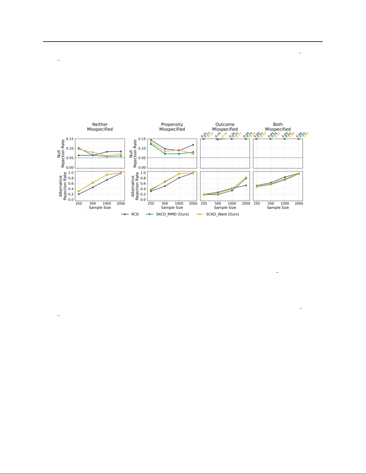
Conditional Distrib utional T r eatment Effects: Doubly Rob ust Estimation and T esting Saksham Jain 1 Alex Luedtke 2 Abstract Beyond conditional average treatment effects, treatments may impact the entire outcome distribution in cov ariate-dependent ways, for e xample, by altering the v ariance or tail risks for speciﬁc subpopulations. W e propose a nov el estimand to capture such conditional distrib utional treatment ef fects, and de velop a doubly robust estimator that is minimax optimal in the local asymptotic sense. Using this, we dev elop a test for the global homogeneity of conditional potential outcome distrib utions that accommodates discrepancies beyond the maximum mean discrepancy (MMD), has prov ably v alid type 1 error , and is consistent against ﬁxed alternativ es—the ﬁrst test, to our knowledge, with such guarantees in this setting. Furthermore, we deriv e exact closed-form expressions for two natural discrepancies (including the MMD), and provide a computationally efﬁcient, permutation-free algorithm for our test. 1. Introduction Causal inference for mean ef fects is well-studied for both mar ginal ( Rosenbaum & Rubin , 1983 ; Robins et al. , 1994 ) and conditional ( Abrev aya et al. , 2015 ; W ager & Athey , 2018 ; K ¨ unzel et al. , 2019 ) estimands, as is their doubly robust estimation ( V an der Laan et al. , 2011 ; Kurz , 2022 ). Howe ver , treatments may impact the entire outcome distribution, a fact that has spurred interest in distributional treatment effects (DTEs) ( Bitler et al. , 2006 ; Chernozhukov et al. , 2013 ; Muandet et al. , 2021 ; Fawk es et al. , 2024 ). Further , these distributional impacts may dif fer across subpopulations, as illustrated in Fig. 1 . Understanding how potential outcome distributions P Y ( a ) | X differ gi ven cov ariates is of signiﬁcant interest ( Chang et al. , 2015 ; Hohber g et al. , 2020 ; Chernozhukov et al. , 2024 ). Kernel methods of fer a rigorous frame work for analyzing DTEs by embedding distrib utions into reproducing kernel Hilbert spaces (RKHSs) ( Song et al. , 2009 ; Gretton et al. , 2012 ) and comparing these embeddings via measures of statistical discrepanc y such as t he MMD, which is zero if and only if the distrib utions are equal, pro vided a characteristic kernel is used ( Sriperumb udur et al. , 2011 ). While inference for marginal DTEs has advanced signiﬁcantly ( Martinez T aboada et al. , 2023 ; Luedtke & Chung , 2024 ), it remains underdev eloped in the conditional setting. Park et al. ( 2021 ) presented a test based on the conditional distributional treatment ef fect associated with the MMD (henceforth referred to as the CoDiTE function) deﬁned as CoDiTE P ( x ) =   µ P Y (1) | X ( x ) − µ P Y (0) | X ( x )   H Y , (1) where µ P Y ( a ) | X ( x ) is the conditional mean embedding ( Park & Muandet , 2020 ) of P Y ( a ) | X ( · | x ) in an RKHS H Y . Howe ver , their estimator for this function is not doubly robust, and they rely on permutation tests that lack validity guarantees. Moreover , other current approaches are either limited to best linear projections ( Kallus & Oprescu , 2023 ) or study testing of pointwise equi v alence ( N ¨ af & Susmann , 2024 ). In this work, we instead focus on globally testing the null of equal conditional potential outcome distributions, H 0 : P Y (1) | X ( · | x ) = P Y (0) | X ( · | x ) P X -a.e. , (2) against the complementary alternati ve. Further discussion of related work is provided in App. B . 1 Department of Statistics, Uni versity of W ashington, Seattle, USA 2 Departments of Health Care Policy and Statistics, Harv ard Univ ersity , USA. Correspondence to: Saksham Jain < sj305@uw .edu > . Pr eprint. Mar ch 18, 2026. 1 Conditional DTEs: DR Estimation and T esting F igur e 1. Simple setting where the conditional av erage treatment effect is null (left) ev en though ther e is DTE heter ogeneity (right). In mor e detail: (left) Scatter plot of X and Y ( a ) , a ∈ { 0 , 1 } , with: X, Y (0) ∼ Unif [ − 1 , 1] independently and Y (1) | X a Unif [ − . 5 , . 5] distribution if X > 0 and a Unif ([ − 1 , − . 5] ∪ [ . 5 , 1]) if X < 0 . (right) Pr oposed witness function for conditional DTE. Our Contributions. 1. W e propose, to our kno wledge, the ﬁrst pro v ably valid kernel-based test for the (global) homogeneity of conditional potential outcome distributions, based on a doubly rob ust estimator . 2. Our test uses the bootstrap to determine a rejection region. In contrast to permutation tests, it does not reﬁt the nuisances across replicates, thereby amortizing computational costs. 3. W e deriv e exact closed-form expressions for MMD and W ald-type test statistics, enabling the construction of W ald-type conﬁdence sets for conditional DTEs. 4. W e construct asymptotically v alid uniform conﬁdence bands to help identify speciﬁc regions of heterogeneous distributional treatment ef fects. 5. W e demonstrate the ﬁnite-sample performance of our methods using both simulations and real-world data. 2. Preliminaries 2.1. Problem Setup W e observe an i.i.d. sample D : = { Z i } n i =1 from a distribution P in a statistical model P on Z : = X × { 0 , 1 } × Y , where Z i : = ( X i , A i , Y i ) comprises pre-treatment cov ariates, a treatment assignment, and outcomes. W e deﬁne the propensity score as π P ( x ) : = P ( A = 1 | X = x ) . Along with the standard causal assumptions (consistenc y , unconfoundedness, ov erlap) ( Stone , 1993 ; Mealli & Rubin , 2003 ), we also assume strong positivity: there exists η > 0 such that for all P ∈ P , η ≤ π P ( x ) ≤ 1 − η P X -a.e. W e assume P is dominated and locally nonparametric. The latter means that the tangent space at each P ∈ P is the Hilbert space L 2 0 ( P ) : = { h ∈ L 2 ( P ) : E P [ h ( Z )] = 0 } ( van der V aart , 2000 ). W e let k and ℓ be bounded characteristic kernels on X and Y with feature maps K x : = k ( x, · ) and L y : = ℓ ( y, · ) , respectiv ely . W e operate in the real, separable tensor product RKHS H : = H X ⊗ H Y associated with the kernel λ (( x, y ) , ( x ′ , y ′ )) : = k ( x, x ′ ) ℓ ( y , y ′ ) . As the product of bounded characteristic kernels, λ is also bounded and characteristic. App. C gives an extended discussion of the full theoretical setup, including formal statements of the causal assumptions and the deﬁnition of the tangent space through quadratic mean differentiability (QMD). For readability , we suppress the explicit dependence of functionals on P (e.g., writing CoDiTE( x ) instead of CoDiTE P ( x ) ) when the value of P is clear from context. 2.2. Conditional Distributional T reatment Effects Under the standard causal assumptions, the conditional mean embedding µ P Y ( a ) | X ( x ) from ( 1 ) is identiﬁed from the observed data by the follo wing H Y -valued function: ν P,a ( x ) : = E P [ L Y | A = a, X = x ] . (3) 2 Conditional DTEs: DR Estimation and T esting Let U P | x : = ν P, 1 ( x ) − ν P, 0 ( x ) . Then, CoDiTE( x ) from ( 1 ) can be e xpressed as ∥ ν P, 1 ( x ) − ν P, 0 ( x ) ∥ H Y =   U P | x   H Y . (4) Park et al. ( 2021 ) use this to dev elop a test for H 0 as in ( 2 ) against the complementary alternati ve. W e show an equiv alent null can be formulated using joint potential outcome and cov ariate distributions instead of conditional distributions. The key argument used to establish this is intuiti ve: since X precedes treatment, the marginal distribution P X must be the same on either side of Eq. 2 —see App. D.1 . Proposition 2.1 (Equi v alent null) . F or any P ∈ P , H 0 holds if and only if P Y (1) ,X = P Y (0) ,X . The conditional mean embedding of the joint potential outcome and cov ariate distrib ution P Y ( a ) ,X is identiﬁed under the standard causal assumptions as the following H -v alued function of x ∈ X deﬁned for each a ∈ { 0 , 1 } : θ P,a ( x ) : = K x ⊗ ν P,a ( x ) . (5) This motiv ates our deﬁnition of the ‘ S moothed’ Co nditional Di stributional T reatment E f fect (SCoDiTE) as the Hilbert-valued parameter ψ : P → H giv en by ψ ( P ) : = E P [ θ P, 1 ( X ) − θ P, 0 ( X )] . (6) W e use the shorthand ψ P : = ψ ( P ) throughout. Consequently , for U P | x ( y ) the witness function for CoDiTE ( x ) from ( 4 ) , the SCoDiTE witness function writes as ψ P ( x, y ) = R k ( x ′ , x ) U P | x ′ ( y ) P X ( dx ′ ) . Thus, ψ P ( · , y ) is an H X -kernel smoothing of U P |· ( y ) . Park et al. ( 2021 ) test H 0 through a criterion they call the kernel conditional discrepanc y: K CD : = E P  CoDiTE 2 ( X )  = E P h   U P | X   2 H Y i . (7) Howe ver , the resulting test statistic is a degenerate two-sample U-statistic under the null, requiring nonparametric estimates of the conditional mean embeddings; it does not admit weak con ver gence to a kno wn distribution in general, prev enting analytical computation of critical values, leading them to use permutation resampling. In contrast, the squared MMD associated with the SCoDiTE is ∥ ψ P ∥ 2 H = E P X E P X h k ( X, X ′ )  U P | X , U P | X ′  H Y i . (8) By cross-correlating the H Y discrepancies rather than squaring them pointwise, it allows us to recast H 0 as the linear moment condition ψ P = 0 ∈ H , expressed in terms of the identiﬁed joint distributions P Y ( a ) ,X . This enables statistically and computationally efﬁcient inference, as we establish rigorously in the follo wing sections. 2.3. Efﬁcient, Doubly-Robust Estimation of the SCoDiTE The classic one-step estimation procedure for a ﬁnite-dimensional parameter ( Pfanzagl , 1982 ) in v olves ‘correcting’ an initial (plug-in) estimate using the so-called ef ﬁcient inﬂuence function (EIF) of that parameter ( Bickel et al. , 1993 ). Howe ver , as the SCoDiTE is Hilbert-v alued, classic one-step estimation is not directly applicable. Consequently , we take inspiration from Luedtke & Chung ( 2024 ) to dev elop a one-step estimator for ψ P . The subsequent lemma is key in accomplishing this, as it prov es the existence of, and e xhibits the form taken by , the EIF of ψ P at each P ∈ P . Before presenting the result, we highlight the main technical challenge underpinning it. Namely , establishing that P 7→ ψ P is pathwise differ entiable relativ e to the statistical model P . W e refer the reader to App. E.1 for the formal presentation of this concept and the subsequent proof. Recall from Sec. 2.1 that π P ( x ) is the propensity to receiv e treatment giv en X = x and θ P,a ( x ) is (a λ -kernelized version of) the outcome model for X = x corresponding to group A = a , both under P . W e no w present the EIF . Lemma 2.2 (Existence and form of the EIF) . The parameter ψ deﬁned as in Eq. 6 is pathwise differ entiable at every P ∈ P , and has an EIF at each P that takes the form ϕ P ( x, a, y ) =  a π P ( x ) − 1 − a 1 − π P ( x )   Λ x,y − θ P,a ( x )  + θ P, 1 ( x ) − θ P, 0 ( x ) − ψ P . Mor eover , 0 < R ∥ ϕ P ( z ) ∥ 2 H P ( dz ) < ∞ for all P ∈ P . 3 Conditional DTEs: DR Estimation and T esting The proof is provided in App. E.2 . Constructing a one-step estimator with the above EIF yields (a λ -kernelized version of) an augmented in verse propensity weighted (AIPW) estimator ( Glynn & Quinn , 2010 ; Hines et al. , 2022 ). T o see this, note that E P [ ϕ ( Z )] = 0 by deﬁnition. Let P n be the empirical distribution induced by the i.i.d. dataset D , and let b P n be an independent (not based on D ) plug-in estimate of P . The one-step estimator is then given by b ψ n : = ψ b P n + E P n  ϕ b P n ( Z )  . In practice, the nuisances π b P n and { θ b P n , 1 , θ b P n , 0 } must be estimated from data. T o av oid o verﬁtting while maintaining statistical efﬁcienc y , we employ cross-ﬁtting ( Schick , 1986 ). Speciﬁcally , let r ∈ { 1 , 2 } denote a data split and ﬁx the complement s : = 3 − r . Let b P r n be an initial estimate of the data-generating distribution based on the data split D r and P s n be the empirical distribution induced by the complementary split D s . W e set the notational con vention of using [ · ] r n instead of [ · ] b P r n . For instance, we let ψ r n denote the plug-in parameter estimate ψ b P r n and ϕ r n the H -valued EIF estimate ϕ b P r n , both of whose nuisances are ﬁtted using D r . Our cross-ﬁtted one-step estimator is then ¯ ψ n : = 1 2 2 X r =1  ψ r n + E P s n [ ϕ r n ( Z )]  . (9) W e emphasize that Lem. 2.2 provides the theoretical basis for establishing the optimality of ¯ ψ n . Indeed, we show in Sec. 3.1 that, under suitable conditions, ¯ ψ n is asymptotically linear . Intuiti vely , this means that ¯ ψ n behav es almost like an empirical mean: it con ver ges to a tight H -valued Gaussian random v ariable at the n − 1 / 2 rate (see Thm. 3.1 and the discussion surrounding it). A key property of our estimator , arising from the form of the EIF , is double rob ustness. Speciﬁcally , ¯ ψ n remains consistent if either the propensity score models { π r n } or the outcome models { θ r n,a } , but not necessarily both, are correctly speciﬁed. W e formalize this property in Sec. 3.1 . 2.4. Permutation-Fr ee, V ariance-A ware Inference The KCD test of H 0 ( 2 ) uses M permutations to ﬁnd the empirical p-value ( Park et al. , 2021 ). Each permutation in v olves reﬁtting the outcome models for both treatment groups. The worst-case computational complexity of their algorithm is O ( M n 3 ) . Since M has been shown to often v ary between 10 2 and 10 3 for performant permutation-based inference ( Davison & Hinkle y , 1997 ), this can quickly become impractical for e ven moderate datasets. W e propose the ‘smoothed’ kernel conditional discrepancy (SKCD) to test the reformulated null H 0 : P Y (1) ,X = P Y (0) ,X against the complementary alternati ve. This statistic takes the following quadratic form: SK CD : = ⟨ Ω P ( ψ P ) , ψ P ⟩ H , (10) where Ω P (to denote potential dependence on P ) is a continuous self-adjoint positi ve-deﬁnite linear H → H operator . It is e vident that when Ω P is the identity operator , SKCD reduces to a squared MMD ( 8 ) . Howe v er , this formulation enables richer discrepancies beyond the MMD. For instance, suppose the appropriately scaled ( ¯ ψ n − ψ P ) con v erges weakly to some H -valued limiting distribution with covariance operator Σ P . T aking Ω P : = [(1 − ε )Σ P + εI ] − 1 yields a kernelized Hotelling-type two-sample T 2 statistic in the spirit of the two-sample test in Eric et al. ( 2007 ), b ut for a cross-ﬁtted one-step estimator in the more complex counterfactual setting. This W ald-type formulation offers higher power when the true effect lies in a low-v ariance subspace of H . T o our knowledge, this paper is the ﬁrst to study this class of discrepancies for a conditional distributional causal estimand. A compelling reason to use SKCD to test H 0 is that it circumvents the need to analytically compute or numerically approximate the asymptotic null distribution of degenerate tw o-sample U-statistics like the KCD. T o see this, ﬁrst note that ψ P = 0 under the null. Let \ SK CD : =  Ω n ( ¯ ψ n ) , ¯ ψ n  H , (11) where Ω n is an appropriate estimator of Ω . Now , if an appropriately scaled ¯ ψ n con v erges weakly to some H -valued limiting distribution under the null that can be analytically derived, then the continuous mapping theorem for Hilbert 4 Conditional DTEs: DR Estimation and T esting random elements immediately yields the limiting null distribution L of the appropriately scaled \ SK CD . This leads to a simple testing procedure: reject H 0 at lev el α when the scaled \ SK CD exceeds the (1 − α ) -quantile of L . Sec. 3.1 details how the quantile can be estimated without r eﬁtting the nuisance models , drastically reducing the computational cost of resampling for inference. In the following section, we establish that the appropriate scaling is n · \ SK CD . W e proceed by rigorously showing that we can (i) analytically deri v e the root- n rate limiting distrib ution of ¯ ψ n , which is optimal in the semiparametric efﬁcienc y (in Hilbert spaces) sense, and (ii) efﬁciently compute both natural SKCD v ariants, the MMD and W ald-type formulations, in closed form for use as test statistics with known limiting distrib utions under the null. 3. Main Results 3.1. Theoretical Guarantees W e henceforth distinguish the true data-generating distribution, denoted by P ⋆ ∈ P , from an arbitrary distribution P ∈ P . W e set the notational con vention to using [ · ] ⋆ instead of [ · ] P ⋆ , e.g., ψ ⋆ denotes the true parameter ( 6 ) under P ⋆ , and π ⋆ , θ ⋆, 0 , and θ ⋆, 1 denote the respectiv e nuisance parameters under P ⋆ , and so on. Let b P r n ∈ P be an initial estimate of P ⋆ computed using the data split D r . The goal in this section is to establish the asymptotic normality of ¯ ψ n ( 9 ) and use it to construct a test of the null, ψ ⋆ = 0 . The analysis hinges on sho wing that ¯ ψ n is asymptotically linear . This property holds if the estimator’ s error , ¯ ψ n − ψ ⋆ , can be written as an empirical a v erage, with any remaining terms v anishing at a faster than n − 1 / 2 rate. Adding zero to ¯ ψ n − ψ ⋆ and rearranging terms yields ¯ ψ n − ψ ⋆ = 1 2 2 X r =1 E P s n [ ϕ ⋆ ( Z )] + 1 2 2 X r =1 ( R r n + D r n ) , (12) where R r n : = ψ r n + E ⋆ [ ϕ r n ( Z )] − ψ ⋆ and D r n : = E P s n [ ϕ r n ( Z ) − ϕ ⋆ ( Z )] − E ⋆ [ ϕ r n ( Z ) − ϕ ⋆ ( Z )] . The following theorem provides suf ﬁcient conditions on the con ver gence rates of the nuisance estimators to ensure that both max r ∥R r n ∥ H and max r ∥D r n ∥ H vanish at the required rate. Slutsky’ s lemma and a Hilbert central limit theorem consequently imply the weak con v ergence of √ n ( ¯ ψ n − ψ ⋆ ) . Theorem 3.1 (W eak con ver gence) . Let ϕ ⋆ be the EIF of ψ at P ⋆ . F or r ∈ { 1 , 2 } , suppose b P r n is such that: (i) ∥ π r n − π ⋆ ∥ L 2 ( P ⋆,X ) = O p ( n − τ r ) for scalar τ r > 0 , (ii)   θ r n,a − θ ⋆,a   L 2 ( P ⋆,X ; H ) = O p ( n − γ a,r ) for scalar γ a,r > 0 for each a ∈ { 0 , 1 } , and (iii) τ r + min { γ 0 ,r , γ 1 ,r } > 1 / 2 . Then, letting ‘ ⇝ ’ denote weak con ver g ence in H , we have 1. ¯ ψ n − ψ ⋆ = 1 n P n i =1 ϕ ⋆ ( Z i ) + o p ( n − 1 / 2 ) , 2. √ n  ¯ ψ n − ψ ⋆  ⇝ H , wher e H is a tight H -valued random variable suc h that ⟨ H , h ⟩ H ∼ N  0 , E ⋆ h ⟨ ϕ ⋆ ( Z ) , h ⟩ 2 H i for every h ∈ H . The proof is provided in App. F .2 . Condition (iii) is a double robustness condition that ensures the remainder R r n con v erges to zero if the product of the nuisance estimation rates goes to zero faster than n − 1 / 2 . The empirical process term D r n is controlled using the consistency of the EIF estimate, which we sho w holds under conditions (i) and (ii). No w we discuss the statistical efﬁciency of our estimator . Since a direct Cram ´ er-Rao lo wer bound does not always e xist in such RKHS settings, we analyze this in a more general framew ork. As we establish in the follo wing theorem, the proposed cross-ﬁtted one-step estimator is asymptotically ef ﬁcient under the conditions of Thm. 3.1 . Intuitively , this means that among the limiting distributions of estimators of ψ ⋆ , the weak limit H of our estimator is optimal in the ‘smallest spread’ sense. W e use the shorthand ψ s,ϵ to mean ψ P s,ϵ . Theorem 3.2 (Local asymptotic minimax optimality) . F or any scor e s ∈ L 2 0 ( P ⋆ ) , let { P s,ϵ } ⊂ P be a QMD submodel 5 Conditional DTEs: DR Estimation and T esting such that P s, 0 = P ⋆ . Deﬁne the local asymptotic minimax risk for an estimator sequence ( ˇ ψ n ) ∞ n =1 as LAMRisk ρ ( ˇ ψ n ; P ⋆ ) : = sup I lim inf n →∞ sup s ∈ I E s, 1 √ n h ρ  √ n h ˇ ψ n − ψ s, 1 √ n ii , wher e ρ : H → R is a nonne gative map, the ﬁrst supremum is over all ﬁnite subsets of L 2 0 ( P ⋆ ) , and the expectation is under the pr oduct measur e P n s, 1 / √ n . Suppose the conditions of Thm. 3.1 hold. Further , let ( e ψ n ) ∞ n =1 be any Bor el- measurable estimator sequence and ρ be any subcon ve x function that is continuous a.s. under the law of H . Pr ovided that the sequence ρ ( √ n ( ¯ ψ − ψ s, 1 / √ n )) is asymptotically uniformly inte gr able under P s, 1 / √ n , we have: LAMRisk ρ ( e ψ n ; P ⋆ ) ≥ E ⋆ [ ρ ( H )] = LAMRisk ρ ( ¯ ψ n ; P ⋆ ) . The proof, presented in App. F .3 , follows from the pathwise differentiability of P 7→ ψ P and the conv olution and minimax theorems for Hilbert-v alued estimators. ( van der V aart & W ellner , 2023 , Theorems 3.12.2 and 3.12.5). The ﬁnal equality is achiev ed via the con ver gence of means for asymptotically uniformly integrable sequences ( van der V aart & W ellner , 2023 , Theorem 1.11.3). W e highlight the relationship between our estimator and existing k ernel-based procedures for mar ginal DTEs. Mar- tinez T aboada et al. ( 2023 ) present a “cross-U-statistic” estimator that relies on a single data split. While it attains the √ n rate, it is asymptotically linear on only half the sample; this results in an ef fectiv e sample size of n/ 2 , precluding local asymptotic minimax optimality ( Kim & Ramdas , 2024 ). In contrast, in a work concurrent to Martinez T aboada et al. ( 2023 ), Luedtke & Chung ( 2024 ) construct a doubly rob ust cross-ﬁtted estimator for marginal DTEs that is asymptotically linear ov er the entire sample, thereby attaining optimality . Our estimator ¯ ψ n is a nontrivial e xtension of this full-sample one-step construction: under the conditions of Theorem 3.1 , it is asymptotically linear in H ov er all n observations, thereby achie ving local asymptotic minimax optimality for conditional DTEs. W e now propose a test for the sharp null hypothesis H 0 : ψ ⋆ = ψ 0 (e.g., ψ 0 = 0 for the null H 0 in Eq. 2 ). Let W denote the set of continuous self-adjoint positiv e-deﬁnite linear operators on H . W e deﬁne our test statistic as T n : = n  Ω n ( ¯ ψ n − ψ 0 ) , ¯ ψ n − ψ 0  H , (13) where Ω n ∈ W is a consistent estimator for a possibly- P ⋆ -dependent operator Ω ⋆ ∈ W (e.g., the identity , or a regularized in v erse cov ariance operator as discussed in Sec. 2.4 ). Note that when ψ 0 = 0 , T n corresponds to n · \ SK CD ( 11 ). W e let submodel P 0 ⊆ P denote the set of all distributions for which the null hypothesis H 0 holds. Under H 0 and consistent estimation of Ω ⋆ , Thm. 3.1 and the continuous mapping theorem imply that T n ⇝ ⟨ Ω ⋆ ( H ) , H ⟩ H . This limiting distribution depends on P ⋆ , which is generally unknown. Therefore, a v alid test re- quires a consistent estimate of the (1 − α ) -quantile of this limit, q α . Alg. 1 bootstraps the empirical mean of the inﬂuence function to compute this estimate, b q n,α . Our test rejects H 0 at lev el α if T n > b q n,α . Algorithm 1 SKCD test via bootstrapping the EIF Input: Data D = { Z i } n i =1 , null ψ 0 (default 0), le vel α , bootstrap samples B , estimate Ω n of operator Ω ⋆ . Split { 1 , . . . , n } into index sets I 1 , I 2 for cross-ﬁtting; Let ¯ ψ n = n − 1 P n i =1 φ i ; Compute ¯ ψ n ( 9 ) and T n ( 13 ); for b = 1 to B do Draw ξ j ∼ Multinomial( n r , 1 /n r , . . . , 1 /n r ) − 1 for j ∈ I r , r ∈ { 1 , 2 } ; Compute ∆ ( b ) n = n − 1 P n i =1 ξ i φ i and T ( b ) n = n D Ω n (∆ ( b ) n ) , ∆ ( b ) n E H ; end for Set b q n,α as (1 − α ) -quantile of { T ( b ) n } B b =1 ; Return: I ( T n > b q n,α ) . Importantly , unlike permutation tests (as in Park et al. , 2021 ) that require reﬁtting nuisance models θ n,a in every permutation, our approach computes the EIF estimates only once. In the bootstrap loop, we simply re-weight these ﬁxed estimates using random, zero-centered multinomial dra ws ξ i to simulate the limit distrib ution H . In fact, for speciﬁc forms of T n (see Sec. 3.2 ), we can amortize all the most expensiv e operations, achie ving a worst-case complexity of 6 Conditional DTEs: DR Estimation and T esting O ( n 3 + B n 2 ) . Compared to a cross-MMD based test (as in Martinez T aboada et al. , 2023 ), our test achie ves optimal asymptotic power while maintaining equi valent complexity , provided that nuisance estimation is super -quadratic. Theorem 3.3 (V alidity of the test in Alg. 1 ) . If the conditions of Thm. 3.1 hold, Ω ⋆ ∈ W , and Ω n ∈ W satisﬁes ∥ Ω n − Ω ⋆ ∥ op = o p (1) , then 1. (type 1 err or contr ol) lim n →∞ P n ⋆ { T n > b q n,α } = α for all P ⋆ ∈ P 0 , and 2. (test consistency) lim n →∞ P n ⋆ { T n > b q n,α } = 1 for any ﬁxed P ⋆ ∈ P \ P 0 . The proof hinges on bootstrap consistency , and is deferred to App. G.1 . While our test provides a decision rule for rejecting the null hypothesis of no global conditional distrib utional effect, it does not immediately re v eal the nature of the heterogeneity upon rejecting the null. T o enable ﬁner interpretation of the SCoDiTE, we can construct a uniform conﬁdence band for the witness function ( x, y ) 7→ ψ ⋆ ( x, y ) by simply inv erting our testing procedure, i.e., by ev aluating the support function of the (1 − α ) -conﬁdence ellipsoid implied by the test. This guarantees uniform cov erage o ver the entire domain Z . When using the W ald-type formulation, our approach adapts the width of the band to the local geometry of the operator Ω n , allowing for tighter bands in regions of the cov ariate space with lower variance. Let W inv ⊂ W consist of all Ω ∈ W that are boundedly inv ertible. Theorem 3.4 (Uniform conﬁdence band for the SCoDiTE) . Suppose the conditions of Thm. 3.1 hold, Ω ⋆ ∈ W inv , and the bootstrap quantile b q n,α is constructed (Alg. 1 ) using Ω n ∈ W inv such that ∥ Ω n − Ω ⋆ ∥ op = o p (1) . De- ﬁne w n : X × Y → R so its squar e satisﬁes w 2 n ( x, y ) : =  Λ x,y , Ω − 1 n Λ x,y  H b q n,α /n , and let B n ( x, y ) : =  ¯ ψ n ( x, y ) − w n ( x, y ) , ¯ ψ n ( x, y ) + w n ( x, y )  . Then, lim n →∞ P n ⋆ ( ψ ⋆ ( x, y ) ∈ B n ( x, y ) for all x, y ) ≥ 1 − α. The proof, provided in App. G.2 , relies on the Cauchy-Schwarz inequality in RKHSs. The band B n allo ws practitioners to visualize the SCoDiTE and helps identify regions of covariates and outcomes where the effect is statistically signiﬁcant. W e can also construct tighter pointwise-in- x uniform-in- y conﬁdence bands by restricting the test statistic in Alg. 1 to H x = { h ( x, · ) : h ∈ H } . W e demonstrate this utility in Sec. 4.2 , where we use these bands to localize wealth impacts for distinct household proﬁles. 3.2. Closed-Form Estimators f or the SKCD W e no w deri ve computable e xpressions for the test statistic. Our constructions are agnostic to the choice of propensity models π r n and accommodate a range of outcome models θ r n,a , including kernel ridge regression, distrib utional random forests ( N ¨ af et al. , 2023 ), and deep kernel methods ( Shimizu et al. , 2024 ), provided these estimates lie in the ﬁnite- dimensional subspace F n : = span { Λ x i ,y j } n i,j =1 . Under this condition, ¯ ψ n lies in F n , and allows the SKCD to be estimated in closed-form using only Gram matrices [ K ] ij = k ( x i , x j ) and [ L ] ij = ℓ ( y i , y j ) . First, for the MMD formulation ( Ω ⋆ = Ω n = I ), we construct a weight matrix. Let β r a ( x ) ∈ R n denote the vector of coefﬁcients for the outcome model θ r n,a ( x ) = P j [ β r a ( x )] j Λ x,y j such that [ β r a ( x )] j = 0 for any observ ation where j / ∈ I r or a j  = a . For an y index i , let s ( i ) ∈ { 1 , 2 } be the split containing i , and r ( i ) = 3 − s ( i ) be the complement. Deﬁne π r ( i ) n ( x i ) : = w i . W e construct C ∈ R n × n entry-wise as: [ C ] ij : =    1 2 n s ( i )  a i w i − 1 − a i 1 − w i  if j = i 1 2 n s ( i ) h  1 − a i w i  [ β r ( i ) 1 ( x i )] j +  1 − a i 1 − w i − 1  [ β r ( i ) 0 ( x i )] j i if j  = i (14) The diagonal terms of C hold in v erse propensity weights, while the off-diagonal block terms capture the augmentation corrections. W ith this representation, the squared RKHS norm of our estimator reduces to a trace operation, as established in the following result. Proposition 3.5 (Closed-form MMD statistic from Alg. 1 ) . If Ω n = I and C is as constructed using ( 14 ) , then the squar ed MMD test statistic fr om Alg. 1 takes the form T MMD n : = n   ¯ ψ n   2 H = n ⟨ C , KCL ⟩ F . W e prove this result in App. H.1 . The MMD statistic can thus be ev aluated with the standard O ( n 3 ) worst-case complexity for kernel methods, ensuring that our test does not incur an extra prohibitive computational ov erhead. 7 Conditional DTEs: DR Estimation and T esting While we focus on exact computation here to isolate statistical performance from approximation errors, we expect that employing lo w - rank kernel approximations (e.g., via the Nystr ¨ om method) would reduce the worst-case complexity below cubic in n under standard conditions on the kernel’ s spectral decay ( Bach , 2013 ; Rudi et al. , 2015 ). W e next turn to the W ald-type statistic, which incorporates the cov ariance structure of the estimator . Let Σ ⋆ ( h ) : = E ⋆ [ ⟨ ϕ ⋆ ( Z ) , h ⟩ H ϕ ⋆ ( Z )] denote the cov ariance operator of H and let Σ n ( h ) : = 1 2 P 2 r =1 E P s n [ ⟨ ϕ r n ( Z ) , h ⟩ H ϕ r n ( Z )] be a ﬁnite-dimensional estimator . The choice of Ω ⋆ corresponds to the re gularized in v erse of Σ ⋆ , and so we consider the ﬁnite-dimensional operator Ω n : = ((1 − ε )Σ n + εI ) − 1 (15) to compute T W ald n . A na ¨ ıve in version on the tensor product space would in v olve an n 2 × n 2 matrix, incurring a prohibitiv e O ( n 6 ) worst-case complexity . T o av oid this, we exploit the fact that the empirical co v ariance Σ n has rank ≤ n , constructing auxiliary matrices that capture the cross-ﬁtting structure and the low-rank factors. Let [ E ] ij represent the pure outcome model coefﬁcients (case 2 of Eq. 14 without the propensity weights). Then, deﬁne: [ D s ] ij : = 1 { i ∈I s } √ 2 n s [ C ] ij , [ V s ] ij : = 1 { i ∈I s } p 2 /n s [ E ] ij , W s : = D s − n s V s . (16) Let d s , v s , w s be the ro w-wise vectorizations of these matrices respecti vely . Deﬁne G : = K ⊗ L , and S s : = (I n • D s ) ⊤ , where ‘ • ’ denotes the ro w-wise Kronecker product. W e stack these components into two block matrices T , U ∈ R n 2 × (2 n +4) as follows: T : =  GS 1 GS 2 Gv 1 Gv 2 Gw 1 Gw 2  , U : =  S 1 S 2 − d 1 − d 2 − v 1 − v 2  . (17) W ith this, the W ald-type statistic reduces to a single-rank correction of the MMD statistic, as established below . Proposition 3.6 (Closed-form W ald-type statistic from Alg 1 ) . If Ω n is as in ( 15 ) and c : = vec( C ⊤ ) is constructed fr om ( 14 ) , then the W ald-type statistic from Alg . 1 can be computed in O ( n 3 ) operations as T W ald n : = n  Ω n ( ¯ ψ n ) , ¯ ψ n  H = n ε ⟨ C , K CL ⟩ F − n (1 − ε ) ε c ⊤ T  ε I + (1 − ε ) U ⊤ T  − 1 U ⊤ Gc . The proof of this result is provided in App. H.2 . The operator Σ n estimates the cov ariance of the EIF in a tensor product RKHS. Consequently , deriving U ⊤ T tractably requires applications of identities in volving face-splitting and Khatri-Rao products. This reduces the dominating computation of T W ald n to in v erting a (2 n + 4) × (2 n + 4) matrix, achieving the same w orst-case complexity as T MMD n . Notably , while Luedtke & Chung ( 2024 ) suggest a test for mar ginal DTEs using their one-step estimator , they do not deriv e closed-form e xpressions for the resulting test statistic; in contrast, our deriv ations enable testing of conditional DTEs while av oiding approximation error . Crucially , these expressions allo w us to further exploit the bilinearity of the inner product in Eq. 13 to pre-compute all objects requiring O ( n 3 ) operations in the SKCD test. Ev aluations within the bootstrap loop simply project the random multipliers onto these pre-computed objects, with each resampling requiring only O ( n 2 ) operations (see App. I ). 4. Experiments 4.1. Simulation: Distribution Shift in Images W e in v estigate the ﬁnite-sample size and power of our SKCD test at level α = 0 . 05 . Our simulation design uses the MNIST dataset ( Deng , 2012 ) to create scenarios where treatment effects manifest as distribution shifts that are challenging to detect. W e let both cov ariates X and outcomes Y be PCA embeddings of learned image representations (in R 5 ) using a ResNet-18-based encoder . T reatment A is assigned via a Bernoulli draw parameterized by a non-linear function of the co variates, designed to maintain overlap. W e provide all e xperimental speciﬁcations and implementation details in App. J.1 . Under the null, outcomes are generated after the images for both groups undergo random intensity changes, ignoring treatment. Under the alternativ e, the treated group images under go an additional rotation whose angle depends non- linearly on X . Thus, the treatment induces a multiv ariate distrib utional effect that is not limited to the mean and v aries with the cov ariates. 8 Conditional DTEs: DR Estimation and T esting W e compare our proposed SKCD test, using both MMD and W ald-type statistics (referred to as SKCD MMD and SKCD Wald respectiv ely), against the baseline KCD test ( Park et al. , 2021 ). W e employ Gaussian kernels for both cov ariate and outcome spaces. All methods use kernel ridge regression for the outcome models and gradient-boosted decision trees for the propensity model. W e e valuate robustness across four regimes: (1) Neither Misspeciﬁed ; (2) Propensity Misspeciﬁed ; (3) Outcome Misspeciﬁed ; and (4) Both Misspeciﬁed . Misspeciﬁcation is achiev ed by withholding the principal components that driv e treatment assignment and ef fect heterogeneity . W e sample a subset of size n ∈ { 250 , 500 , 1000 , 2000 } from the simulated data { X i , A i , Y i } 45 k i =1 with replacement. The plots in Fig. 2 report the rejection rates at le vel α = 0 . 05 for 1000 Monte Carlo (MC) replicates of each experimental conﬁguration for all three tests under consideration. F igur e 2. T ype 1 error and power at α = 0 . 05 across sample sizes and nuisance misspeciﬁcation regimes. (Left) Scenario satisfying asymptotic guarantees (the product of nuisance estimation errors is o p ( n − 1 / 2 ) ). (Right) Robustness checks under model misspeciﬁcation. The proposed tests beneﬁt from double robustness of the estimator; type 1 error is closer than baseline to the nominal le vel under propensity misspeciﬁcation; under outcome misspeciﬁcation, type 1 error is inﬂated but stable, while power increases with sample size. In the Neither Misspeciﬁed regime, the proposed SKCD test variants show slightly inﬂated type 1 error at smaller sample sizes that—consistent with our theory—approaches nominal as sample size grows. SKCD MMD achiev es type 1 error quite close to nominal e ven in the Pr opensity Misspeciﬁed regime, while the baseline KCD suffers signiﬁcant inﬂation. Even in the Outcome Misspeciﬁed setting, where type 1 error control is challenging, both SKCD vari ants prov e notably more stable than KCD , which div er ges sharply as n increases. Under the alternativ e hypothesis, power increases with sample size across all (v alid) conﬁgurations; ho wev er , our proposed methods consistently outperform KCD . This is most visible in the Outcome Misspeciﬁed regime, where (though under inﬂated type 1 error) both SKCD MMD and SKCD Wald achiev e ∼ 80% power at n = 2000 while the baseline plateaus. Additional experiments in App. A using known propensity scores sho w that all methods achie ve nominal type I error control when correctly speciﬁed, while the observed adv antages of both SKCD variants o v er KCD under outcome misspeciﬁcation become ev en more pronounced. T o assess our double robustness guarantee for the estimator ¯ ψ n ( 9 ) , we analyze its conv er gence under the null ( ψ ⋆ = 0 ). In App. A , we plot its empirical mean squared error (MSE) in the RKHS norm, i.e., the a v erage of ∥ ¯ ψ n ∥ 2 H = n − 1 T MMD n across MC replicates. W e observe that the MSE decreases sharply with increase in n if ev en one nuisance model is correctly speciﬁed, consistent with our theory . 4.2. Real Data: Impact of 401(k) Eligibility on Household W ealth W e apply our methods to W ave 4 ( 9 , 915 households) of the 1990 Surve y of Income and Program P articipation ( Cher- nozhukov & Hansen , 2004 ; Benjamin , 2003 ; Gelber , 2011 ; Kallus & Oprescu , 2023 ) to study the effect of 401(k) eligibility ( A ) on household wealth. All e xperimental speciﬁcations and implementation details are pro vided in App. J.2 Follo wing recent work ( N ¨ af & Susmann , 2024 ), we analyze a multiv ariate outcome Y ∈ R 3 comprising Net Financial Assets (TF A), Net non-401(k) Assets (NIF A), and T otal W ealth (TW). The pre-treatment cov ariates X comprise four continuous features—age, income, f amily size, education, and ﬁ v e categorical—deﬁned - beneﬁt plan, marital status, dual earner , IRA participation, and home o wnership. 9 Conditional DTEs: DR Estimation and T esting F igur e 3. Estimated witness functions with 95% uniform conﬁdence bands for tw o household proﬁles (ro ws) across three wealth outcomes (columns; in 1 k ). Shaded regions indicate statistical signiﬁcance. While Proﬁle 1 exhibits a distributional shift along the ﬁrst axis, Proﬁle 2 shows no detectable ef fect. The proposed SKCD test rejects the global null H 0 : P Y (1) ,X = P Y (0) ,X at lev el α = 0 . 05 . Extending the analysis, we construct 95% uniform-in- y conﬁdence bands for the SCoDiTE witness function ψ ⋆ ( x, · ) by adapting the construction from Thm. 3.4 to the RKHS slice { h ( x, · ) : h ∈ H } . Due to the infeasibility of visualizing the full 3D witness function surface ov er Y , we compute 1D cross-sections by varying each wealth component Y j ov er its support while ﬁxing the other two at their sample means. This allows us to localize the detectable ef fect to speciﬁc re gions of the outcome space for household proﬁles characterized by x . Fig. 3 displays these witness function cross-sections for two distinct households that illustrate the effect heterogeneity . Individual 1 (top) is a 58-year -old individual with moderate income ($30.3k), in a family of size 1, with high education (18 years), possessing an IRA and a deﬁned-beneﬁt plan. Individual 2 (bottom) is a 36-year-old indi vidual with similar income ($34k) but a lar ge family (size 13), lo w education (4 years), and no other retirement plans. For Indi vidual 1, the conﬁdence band along the ﬁrst wealth measure excludes zero ov er signiﬁcant regions. In particular , the estimated witness function for Net Financial Assets exhibits a neg ati ve-to-positi v e swing. This suggests that, holding other assets at their av erage levels, 401(k) eligibility shifts the distribution of ﬁnancial assets for this demographic: reducing the density of low asset v alues and increasing the density of high asset values. For Individual 2, the estimated witness function cross-sections are essentially ﬂat, and the conﬁdence bands contain zero across the entire domain of each wealth measure, providing no e vidence of wealth impact from 401(k) eligibility . 5. Discussion W e introduce the SCoDiTE framework, bridging kernel mean embeddings and semiparametric efﬁcienc y theory to rigorously test for conditional distrib utional treatment ef fects. W e provide the ﬁrst doubly robust, asymptotically optimal estimator for this setting, along with a permutation-free test for valid inference, for which we derive MMD and W ald-type test statistics in closed form. Future work could focus on extending this frame work to continuous treatments or instrumental variable settings. Furthermore, while our W ald-type statistic improv es power , data-driv en selection of the regularization parameter ε remains an open problem. Finally , appropriately incorporating kernel approximation methods into our closed-form expressions would allo w their application to massive datasets. Acknowledgments This work was supported by the Patient Centered Outcomes Research Initiativ e (PCORI, ME-2024C2-39990). The content is solely the responsibility of the authors and does not necessarily represent the of ﬁcial vie ws of the funding agency . 10 Conditional DTEs: DR Estimation and T esting References Abrev aya, J., Hsu, Y .-C., and Lieli, R. P . Estimating conditional average treatment effects. Journal of Business & Economic Statistics , 33(4):485–505, 2015. Akiba, T ., Sano, S., Y anase, T ., Ohta, T ., and Koyama, M. Optuna: A next-generation hyperparameter optimization framew ork. In Proceedings of the 25th ACM SIGKDD international conference on knowledge discovery & data mining , pp. 2623–2631, 2019. Bach, F . Sharp analysis of low-rank kernel matrix approximations. In Confer ence on learning theory , pp. 185–209. PMLR, 2013. Balasubramanian, K., Li, T ., and Y uan, M. On the optimality of kernel-embedding based goodness-of-ﬁt tests. Journal of Machine Learning Resear ch , 22(1):1–45, 2021. Benjamin, D. J. Does 401 (k) eligibility increase saving?: Evidence from propensity score subclassiﬁcation. Journal of Public Economics , 87(5-6):1259–1290, 2003. Bickel, P . J., Klaassen, C. A., Bickel, P . J., Ritov , Y ., Klaassen, J., W ellner , J. A., and Rito v , Y . Efﬁcient and adaptive estimation for semiparametric models , v olume 4. Johns Hopkins Univ ersity Press Baltimore, 1993. Bitler , M. P ., Gelbach, J. B., and Hoynes, H. W . What mean impacts miss: Distributional effects of welfare reform experiments. American Economic Revie w , 96(4):988–1012, 2006. Chang, M., Lee, S., and Whang, Y .-J. Nonparametric tests of conditional treatment effects with an application to single-sex schooling on academic achie v ements. The Econometrics Journal , 18(3):307–346, 2015. Chernozhukov , V . and Hansen, C. The effects of 401 (k) participation on the wealth distribution: an instrumental quantile regression analysis. Revie w of Economics and statistics , 86(3):735–751, 2004. Chernozhukov , V ., Fern ´ andez-V al, I., and Melly , B. Inference on counterfactual distrib utions. Econometrica , 81(6): 2205–2268, 2013. Chernozhukov , V ., Fernandez-V al, I., and W eidner , M. Network and panel quantile ef fects via distrib ution regression. Journal of Econometrics , 240(2):105009, 2024. Davison, A. C. and Hinkle y , D. V . Bootstrap methods and their application . Number 1 in Cambridge Series in Statistical and Probabilistic Mathematics. Cambridge univ ersity press, 1997. Deng, L. The mnist database of handwritten digit images for machine learning research. IEEE Signal Pr ocessing Magazine , 29(6):141–142, 2012. Eric, M., Bach, F ., and Harchaoui, Z. T esting for homogeneity with kernel ﬁsher discriminant analysis. Advances in Neural Information Pr ocessing Systems , 20, 2007. Fa wkes, J., Hu, R., Ev ans, R. J., and Sejdino vic, D. Doubly robust kernel statistics for testing distrib utional treatment effects. T ransactions on Machine Learning Resear ch , 2024. Fukumizu, K., Gretton, A., Lanckriet, G., Sch ¨ olkopf, B., and Sriperumbudur , B. K. K ernel choice and classiﬁability for rkhs embeddings of probability distributions. Advances in neural information pr ocessing systems , 22, 2009. Gelber , A. M. How do 401 (k) s affect saving? evidence from changes in 401 (k) eligibility . American Economic Journal: Economic P olicy , 3(4):103–122, 2011. Glynn, A. N. and Quinn, K. M. An introduction to the augmented inv erse propensity weighted estimator . P olitical analysis , 18(1):36–56, 2010. Gretton, A., Borgw ardt, K. M., Rasch, M. J., Sch ¨ olkopf, B., and Smola, A. A kernel tw o-sample test. The Journal of Machine Learning Resear ch , 13(1):723–773, 2012. Hines, O., Duk es, O., Diaz-Ordaz, K., and V ansteelandt, S. Demystifying statistical learning based on efﬁcient inﬂuence functions. The American Statistician , 76(3):292–304, 2022. 11 Conditional DTEs: DR Estimation and T esting Hohberg, M., P ¨ utz, P ., and Kneib, T . Treatment ef fects be yond the mean using distributional re gression: Methods and guidance. PloS one , 15(2):e0226514, 2020. Kallus, N. and Oprescu, M. Robust and agnostic learning of conditional distrib utional treatment effects. In International Confer ence on Artiﬁcial Intelligence and Statistics , pp. 6037–6060. PMLR, 2023. Ke, G., Meng, Q., Finle y , T ., W ang, T ., Chen, W ., Ma, W ., Y e, Q., and Liu, T .-Y . Lightgbm: A highly efﬁcient gradient boosting decision tree. Advances in neural information pr ocessing systems , 30, 2017. Kim, I. and Ramdas, A. Dimension-agnostic inference using cross u-statistics. Bernoulli , 30(1):683–711, 2024. K ¨ ubler , J. M., Jitkrittum, W ., Sch ¨ olkopf, B., and Muandet, K. A witness two-sample test. In International Conference on Artiﬁcial Intelligence and Statistics , pp. 1403–1419. PMLR, 2022. K ¨ unzel, S. R., Sekhon, J. S., Bickel, P . J., and Y u, B. Metalearners for estimating heterogeneous treatment effects using machine learning. Pr oceedings of the national academy of sciences , 116(10):4156–4165, 2019. Kurz, C. F . Augmented in v erse probability weighting and the double robustness property . Medical Decision Making , 42(2):156–167, 2022. Luedtke, A. and Chung, I. One-step estimation of differentiable Hilbert-v alued parameters. The Annals of Statistics , 52 (4):1534 – 1563, 2024. doi: 10.1214/24- A OS2403. URL https://doi.org/10.1214/24- AOS2403 . Martinez T aboada, D., Ramdas, A., and Kennedy , E. An efﬁcient doubly-robust test for the kernel treatment effect. Advances in Neural Information Pr ocessing Systems , 36:59924–59952, 2023. Mealli, F . and Rubin, D. B. Assumptions allowing the estimation of direct causal effects. J ournal of Econometrics , 112 (1):79–87, 2003. Muandet, K., Kanagawa, M., Saengkyongam, S., and Marukatat, S. Counterfactual mean embeddings. J ournal of Machine Learning Resear ch , 22(162):1–71, 2021. Mukherjee, S. and Sriperumb udur , B. K. Minimax optimal kernel two-sample tests with random features. arXiv pr eprint arXiv:2502.20755 , 2025. N ¨ af, J. and Susmann, H. Causal-drf: Conditional kernel treatment effect estimation using distrib utional random forest. arXiv pr eprint arXiv:2411.08778 , 2024. N ¨ af, J., Emmenegger , C., B ¨ uhlmann, P ., and Meinshausen, N. Conﬁdence and uncertainty assessment for distributional random forests. Journal of Machine Learning Resear ch , 24(366):1–77, 2023. Park, J. and Muandet, K. A measure-theoretic approach to kernel conditional mean embeddings. Advances in neural information pr ocessing systems , 33:21247–21259, 2020. Park, J., Shalit, U., Sch ¨ olkopf, B., and Muandet, K. Conditional distributional treatment ef fect with kernel conditional mean embeddings and u-statistic regression. In International confer ence on machine learning , pp. 8401–8412. PMLR, 2021. Petersen, K. B., Pedersen, M. S., et al. The matrix cookbook. T echnical University of Denmark , 7(15):510, 2008. Pfanzagl, J. Lecture notes in statistics. Contributions to a g eneral asymptotic statistical theory , 13:11–15, 1982. Poterba, J. M. and V enti, S. F . 401 (k) plans and tax-deferred saving. In Studies in the Economics of Aging , pp. 105–142. Univ ersity of Chicago Press, 1994. Rao, C. R. Estimation of heteroscedastic v ariances in linear models. J ournal of the American Statistical Association , 65 (329):161–172, 1970. Robins, J. M., Rotnitzky , A., and Zhao, L. P . Estimation of regression coefﬁcients when some regressors are not alw ays observed. Journal of the American statistical Association , 89(427):846–866, 1994. 12 Conditional DTEs: DR Estimation and T esting Rosenbaum, P . R. and Rubin, D. B. The central role of the propensity score in observational studies for causal ef fects. Biometrika , 70(1):41–55, 1983. Roth, W . E. On direct product matrices. 1934. Rudi, A., Camoriano, R., and Rosasco, L. Less is more: Nystr ¨ om computational regularization. Advances in neur al information pr ocessing systems , 28, 2015. Schick, A. On asymptotically efﬁcient estimation in semiparametric models. The Annals of Statistics , pp. 1139–1151, 1986. Shimizu, E., Fukumizu, K., and Sejdinovic, D. Neural-kernel conditional mean embeddings. arXiv pr eprint arXiv:2403.10859 , 2024. Slyusar , V . A family of face products of matrices and its properties. Cybernetics and systems analysis , 35(3):379–384, 1999. Song, L., Huang, J., Smola, A., and Fukumizu, K. Hilbert space embeddings of conditional distributions with applications to dynamical systems. In Pr oceedings of the 26th Annual International Confer ence on Machine Learning , pp. 961–968, 2009. Sriperumbudur , B. K., Fukumizu, K., and Lanckriet, G. R. Univ ersality , characteristic kernels and rkhs embedding of measures. Journal of Machine Learning Resear ch , 12(7), 2011. Stone, R. The assumptions on which causal inferences rest. Journal of the Royal Statistical Society Series B: Statistical Methodology , 55(2):455–466, 1993. V an der Laan, M. J., Rose, S., et al. T arg eted learning: causal inference for observational and experimental data , volume 4. Springer , 2011. van der V aart, A. and W ellner , J. W eak Conver gence and Empirical Processes: W ith Applications to Statistics . Springer New Y ork, 2023. doi: 10.1007/978- 3- 031- 29040- 4. van der V aart, A. W . Asymptotic statistics , volume 3. Cambridge uni versity press, 2000. W ager , S. and Athe y , S. Estimation and inference of heterogeneous treatment effects using random forests. Journal of the American Statistical Association , 113(523):1228–1242, 2018. 13 Conditional DTEs: DR Estimation and T esting A ppendix A Additional Experiments 15 B Extended Related W ork 15 C Extended Problem Setup 15 D Formulating the Estimand 17 D.1 Proof of Proposition 2.1 . . . . . . . . . . . . . . . . . . . . . . . . . . . . . . . . . . . . . . . . . . 17 E Derivation of the EIF 17 E.1 Pathwise Differentiability of ψ P . . . . . . . . . . . . . . . . . . . . . . . . . . . . . . . . . . . . . 17 E.2 Proof of Lemma 2.2 . . . . . . . . . . . . . . . . . . . . . . . . . . . . . . . . . . . . . . . . . . . . 21 F W eak Con vergence and Efﬁciency of ¯ ψ n 25 F .1 Supporting T echnical Results . . . . . . . . . . . . . . . . . . . . . . . . . . . . . . . . . . . . . . . 25 F .2 Proof of Theorem 3.1 . . . . . . . . . . . . . . . . . . . . . . . . . . . . . . . . . . . . . . . . . . . 30 F .3 Proof of Theorem 3.2 . . . . . . . . . . . . . . . . . . . . . . . . . . . . . . . . . . . . . . . . . . . 30 G Guarantees f or the SKCD test 32 G.1 Proof of Theorem 3.3 . . . . . . . . . . . . . . . . . . . . . . . . . . . . . . . . . . . . . . . . . . . 32 G.2 Proof of Theorem 3.4 . . . . . . . . . . . . . . . . . . . . . . . . . . . . . . . . . . . . . . . . . . . 34 H T est Statistics in Closed-Form 35 H.1 MMD Formulation . . . . . . . . . . . . . . . . . . . . . . . . . . . . . . . . . . . . . . . . . . . . 36 H.1.1 Supporting Lemma . . . . . . . . . . . . . . . . . . . . . . . . . . . . . . . . . . . . . . . . 36 H.1.2 Proof of Proposition 3.5 . . . . . . . . . . . . . . . . . . . . . . . . . . . . . . . . . . . . . 36 H.2 W ald-type Formulation . . . . . . . . . . . . . . . . . . . . . . . . . . . . . . . . . . . . . . . . . . 37 H.2.1 Supporting Lemmas . . . . . . . . . . . . . . . . . . . . . . . . . . . . . . . . . . . . . . . 37 H.2.2 Proof of Proposition 3.6 . . . . . . . . . . . . . . . . . . . . . . . . . . . . . . . . . . . . . 41 H.2.3 Heuristic for choosing ε . . . . . . . . . . . . . . . . . . . . . . . . . . . . . . . . . . . . . 42 I Fast SKCD T est Implementation 43 J Experimental Details 45 J.1 Distrib ution shift in images . . . . . . . . . . . . . . . . . . . . . . . . . . . . . . . . . . . . . . . . 45 J.2 Real Data: 401k eligibility . . . . . . . . . . . . . . . . . . . . . . . . . . . . . . . . . . . . . . . . 48 14 Conditional DTEs: DR Estimation and T esting A. Additional Experiments F igur e 4. Empirical MSE of the SCoDiTE estimator ¯ ψ n under the global null, across sample sizes and model misspeciﬁcatiom regimes. ( Left three panels ) The MSE decays sharply to zero when at least one of the nuisance models is correctly speciﬁed. ( Rightmost panel ) The MSE decays at a much slower rate when both propensity and outcome models are simultaneously misspeciﬁed. F igur e 5. T ype 1 error and power at α = 0 . 05 across sample sizes when propensity scores are known. (Left) The outcome model is correctly speciﬁed. (Right) The outcome model is misspeciﬁed. Since the propensity scores are known, the product of nuisance estimation errors is o p ( n − 1 / 2 ) in both scenarios. Thus, in contrast to the baseline, type 1 error is controlled at the nominal lev el and power increases with sample size e v en under outcome misspeciﬁcation. B. Extended Related W ork Muandet et al. ( 2021 ) introduced kernel-based marginal DTE estimators. Fawk es et al. ( 2024 ) dev eloped MMD-based doubly robust test statistics for marginal DTEs though the y did not pro vide complete theoretical guarantees such as type 1 error control for inference. Martinez T aboada et al. ( 2023 ) provided a test based on a doubly rob ust estimator to test marginal DTEs b ut their estimator incurs a loss in asymptotic ef ﬁciency relati ve to an optimal estimator by a factor of √ 2 due to their sample splitting-based approach. Luedtke & Chung ( 2024 ) dev eloped a one-step estimator for testing marginal DTEs that a v oids this penalty , but did not deri ve closed-form test statistics or consider conditional DTEs. Eric et al. ( 2007 ) proposed a kernelized Hotelling’ s T 2 statistic using a plug-in regularized in v erse cov ariance operator for standard two-sample testing. More recently , this framework has been studied for goodness-of-ﬁt testing ( Bala- subramanian et al. , 2021 ) and distrib ution shifts ( K ¨ ubler et al. , 2022 ; Mukherjee & Sriperumbudur , 2025 ). Howev er , these approaches are restricted to non-causal settings: K ¨ ubler et al. ( 2022 ) use a two-stage (train/test split) procedure to construct a precision-weighted witness, while Mukherjee & Sriperumb udur ( 2025 ) use random features to achie v e minimax optimality in the standard two-sample problem. T o the best of our knowledge, such W ald-type discrepancies hav e not been extended to the conditional distrib utional causal setting C. Extended Problem Setup Let P be the statistical model, a collection of distributions on a space Z . W e assume Z is a Polish space deﬁned as Z : = X × A × Y , where A : = { 0 , 1 } , equipped with its Borel σ -algebra B Z ≡ B X ⊗ B A ⊗ B Y . W e observe an i.i.d. 15 Conditional DTEs: DR Estimation and T esting sample D : = { Z i } n i =1 , Z i : = ( X i , A i , Y i ) ∼ P ∈ P , where X i ∈ X are cov ariates, A i ∈ { 0 , 1 } is the treatment, and Y i ∈ Y is the outcome. For a gi ven P ∈ P , we denote the marginal distribution of X by P X and the conditional distribution of Y giv en ( A, X ) by P Y | A,X . W e assume P Y | A,X is non-degenerate. W e denote the conditional probability mass function of the treatment A giv en X = x by g P ( · | x ) , and deﬁne the propensity score as π P ( x ) : = g P (1 | x ) = P ( A = 1 | X = x ) . W e assume the model P is dominated by a σ -ﬁnite measure µ . For each P ∈ P , we let L 2 ( P ) denote the usual Hilbert space of P -square-integrable real-v alued functions on Z with inner product ⟨ h 1 , h 2 ⟩ L 2 ( P ) : = R h 1 h 2 dP . W e now state a smoothness assumption required for the model to support semiparametric ef ﬁciency theory . A submodel { P ϵ ∈ P : ϵ > 0 } is called quadratic mean dif ferentiable (QMD) at P ∈ P if there exists a score function s ∈ L 2 ( P ) such that E P [ s ( Z )] = 0 and     √ p ϵ − √ p − 1 2 ϵs √ p     L 2 ( µ ) = o ( ϵ ) , (18) where p ϵ : = dP ϵ /dµ and p : = dP /dµ . The set of all such scores s , taken ov er all possible QMD submodels at P , forms the tangent set at P . Its closed linear span is the tangent space. Finally , we assume that P is locally nonparametric. Speciﬁcally , for each P ∈ P , that means the tangent space is the entire set of centered square-inte grable functions: L 2 0 ( P ) : = { h ∈ L 2 ( P ) : E P [ h ( Z )] = 0 } . Throughout, we assume that the tangent set is equal to the tangent space. Causal identiﬁcation assumptions. The conditional mean embedding µ P Y ( a ) | X is identiﬁed with ν P,a as deﬁned in ( 3 ) under the following standard assumptions ( Stone , 1993 ; Mealli & Rubin , 2003 ): 1. Consistency: Y = AY (1) + (1 − A ) Y (0) . 2. Unconfoundedness: Y ( a ) ⊥ ⊥ A | X for a ∈ { 0 , 1 } . 3. Overlap: 0 < π P ( x ) < 1 for all x ∈ X . In addition to the identiﬁcation conditions above, we impose str ong positivity : the propensity scores π P are P X -a.e. bounded away from 0 and 1 uniformly over P ∈ P . Speciﬁcally , there exists η > 0 such that for all P ∈ P , η ≤ π P ( x ) ≤ 1 − η for P X -almost all x . RKHS structure. W e utilize the following RKHSs: • H Y : Associated with a bounded characteristic kernel ℓ : Y × Y → R and feature map L y : = ℓ ( y , · ) . • H X : Associated with a bounded characteristic kernel k : X × X → R and feature map K x : = k ( x, · ) . • H : The tensor product RKHS H : = H X ⊗ H Y ( Park & Muandet , 2020 ). This space is associated with the product kernel λ (( x, y ) , ( x ′ , y ′ )) : = k ( x, x ′ ) ℓ ( y , y ′ ) and has the feature map Λ x,y = K x ⊗ L y . Since k and ℓ are bounded and characteristic, the product kernel λ is also bounded and characteristic. W e assume throughout that H is real and separable. Notational remark for proofs. W e will frequently omit the tensor product notation ⊗ to declutter math displays. For instance, we will often write the feature map Λ x,y = K x ⊗ L y as K x L y . Similarly , the kernel λ (( x, y ) , ( x ′ , y ′ )) may appear as k ( x, x ′ ) ℓ ( y , y ′ ) . When manipulating terms in v olving our one-step estimator , we will often rely on the bilinearity of the tensor product to factorize expressions, and will then omit ⊗ . For example, the term a π P ( x ) ( K x ⊗ L y − K x ⊗ ν P,a ( x )) may be written more compactly as a π P ( x ) K x ( L y − ν P,a ( x )) . This should be interpreted strictly as the tensor product of the element K x ∈ H X with the element ( L y − ν P,a ( x )) ∈ H Y . 16 Conditional DTEs: DR Estimation and T esting D. F ormulating the Estimand In this appendix, we justify the formulation of our estimand, the SCoDiTE, by showing that testing for conditional distributional in variance is equi v alent to testing for the equality of joint distributions P Y ( a ) ,X for a ∈ { 0 , 1 } . D.1. Pr oof of Pr oposition 2.1 In the potential outcomes framew ork, X is pre -treatment. This is key for the follo wing proof. Proposition 2.1 (Equi v alent null) . F or any P ∈ P , H 0 holds if and only if P Y (1) ,X = P Y (0) ,X . Pr oof. Suppose H 0 holds. For all a ∈ { 0 , 1 } and Borel-measurable B ⊆ Y and C ⊆ X , it holds that P Y ( a ) ,X ( B × C ) = Z C Z B P Y ( a ) | X ( dy | x ) P X ( dx ) . Note that the disintegration theorem guarantees the uniqueness of conditional distrib utions in e very Polish space equipped with its Borel σ -algebra. Now , if P Y (1) | X ( · | x ) = P Y (0) | X ( · | x ) P X -a.e., then direct substitution of the abov e yields P Y (1) ,X ( B × C ) = Z C Z B P Y (1) | X ( dy | x ) P X ( dx ) = Z C Z B P Y (0) | X ( dy | x ) P X ( dx ) = P Y (0) ,X ( B × C ) . Since this holds for all measurable Cartesian products B × C , which form a π -system that generates the product σ -algebra, we conclude by the π - λ theorem that P Y (1) ,X = P Y (0) ,X . W e no w establish the other direction. Suppose P Y (1) ,X = P Y (0) ,X . For any Borel-measurable sets B ⊆ Y and C ⊆ X , P Y (1) ,X = P Y (0) ,X and the law of total e xpectation together yield 0 = P Y (1) ,X ( B × C ) − P Y (0) ,X ( B × C ) = Z C  P Y (1) | X ( B | x ) − P Y (0) | X ( B | x )  P X ( dx ) . Since this must hold for any measurable set C ⊆ X , we hav e that P Y (1) | X ( B | x ) = P Y (0) | X ( B | x ) P X -almost all x . Thus, for any ﬁx ed set B , there exists a null set N B ⊆ X such that: P Y (1) | X ( B | x ) = P Y (0) | X ( B | x ) for all x / ∈ N B . Let G be a countable π -system that generates the Borel σ -algebra on Y . Let N = S B ′ ∈G N B ′ , and note that as a countable union of null sets, N is also a null set. Now , for any x / ∈ N , it holds that P Y (1) | X ( B ′ | x ) = P Y (0) | X ( B ′ | x ) for all B ′ ∈ G . Thus, we conclude that P Y (1) | X ( · | x ) = P Y (0) | X ( · | x ) for P X -almost all x by appealing again to the π - λ theorem. E. Derivation of the EIF W e use a one-step estimator of SCoDiTE, based on its nonparametric EIF . Here we establish the e xistence and functional form of that object. E.1. Pathwise Differ entiability of ψ P The RKHS-valued SCoDiTE parameter P 7→ ψ P ( 6 ) will hav e an EIF if it is pathwise differentiable and a moment condition is satisﬁed. W e begin by establishing pathwise dif ferentaibility . Let { P ϵ : ϵ ∈ [0 , δ ) } ⊂ P be a QMD submodel passing through P ∈ P at ϵ = 0 with score function s ∈ L 2 0 ( P ) . Let P ( P , P , s ) be the set of all such submodels. A parameter ψ : P → H is pathwise differentiable at P relativ e to the locally nonparametric model P if and only if there exists a continuous linear operator ˙ ψ P : L 2 0 ( P ) → H such that for all s ∈ L 2 0 ( P ) and e very { P ϵ } ∈ P ( P, P , s ) ,    ψ P ϵ − ψ P − ϵ ˙ ψ P ( s )    H = o ( ϵ ) . (19) 17 Conditional DTEs: DR Estimation and T esting The operator ˙ ψ P is referred to as the local parameter or pathwise deriv ative of ψ at P . Let ψ P,a : = E P E P [Λ X,Y | A = a, X ] . Then, by linearity of expectation, our estimand ψ P ( 6 ) decomposes as ψ P = ψ P, 1 − ψ P, 0 . (20) T o establish the pathwise dif ferentiability of ψ P , we can ﬁrst establish it for ψ P, 1 , appeal to symmetry of the binary treatment, and then use the triangle inequality to conclude the argument. T o this end, we leverage an e xisting result for the counterfactual kernel mean embedding (CKME) of a generic distribution Q on X × { 0 , 1 } × W ; in our subsequent arguments, Q will be the distribution of ( X, A, W := ( X , Y )) under sampling ( X, A, Y ) ∼ P . Lemma E.1 (Pathwise differentiability of the CKME) . Let Q be a locally nonpar ametric model comprising distributions on Z : = X × { 0 , 1 } × W satisfying str ong positivity , wher e W is a P olish space equipped with a bounded c haracteristic kernel k W and associated RKHS H W with featur e map Φ w : = k W ( w , · ) . The parameter µ a : Q → H W deﬁned by µ a ( Q ) : = E Q [ E Q [Φ W | A = a, X ]] is pathwise differ entiable at any Q ∈ Q . Its local parameter at scor e s ∈ L 2 0 ( Q ) is given by ˙ µ Q,a ( s ) : = Z Z Φ w  s W | A,X ( w | a, x ) + s X ( x )  Q W | A,X ( dw | a, x ) Q X ( dx ) , (21) wher e s W | A,X and s X ar e the conditional and mar ginal score components deﬁned as s W | A,X ( w | a, x ) : = s ( z ) − E Q [ s ( Z ) | A = a, X = x ] and s X ( x ) : = E Q [ s ( Z ) | X = x ] . Pr oof. See Appendix B.4.1 of Luedtk e & Chung ( 2024 ), speciﬁcally the deri v ation of Eq. 19 and the veriﬁcation of conditions for Lemma 2 therein. Their proof ultimately relies on the boundedness of the kernel and strong positi vity , which are both satisﬁed here. Next, we establish that quadratic mean differentiability (QMD) and pathwise differentiability are preserved when pushed forward through an injecti ve map. Lemma E.2 (In v ariance under injecti v e pushforwards) . Let ( Z , B Z ) and ( ˜ Z , B ˜ Z ) be P olish spaces. Let T : Z → ˜ Z be a measurable injection suc h that T − 1 is measurable on the r ange T ( Z ) . F or a locally nonparametric model P on Z , deﬁne the induced model Q : = { P ◦ T − 1 : P ∈ P } on ˜ Z , noting that each Q ∈ Q is supported on T ( Z ) . (i) If a submodel { P ϵ } ⊂ P is QMD at P with scor e s ∈ L 2 0 ( P ) , then the induced submodel { Q ϵ : = P ϵ ◦ T − 1 } ⊂ Q is QMD at Q : = P ◦ T − 1 with scor e ˜ s : = s ◦ T − 1 ∈ L 2 0 ( Q ) . (ii) Let H be the action space and let ˜ ψ : Q → H be a parameter . Deﬁne ψ : P → H by ψ ( P ) : = ˜ ψ ( P ◦ T − 1 ) . If ˜ ψ is pathwise differ entiable at Q with local parameter ˙ ˜ ψ Q , then ψ is pathwise differ entiable at P with local parameter ˙ ψ P ( s ) : = ˙ ˜ ψ P ◦ T − 1 ( s ◦ T − 1 ) . Pr oof. Let µ be a σ -ﬁnite measure dominating the model P . Deﬁne the pushforward measure on ˜ Z by ˜ µ : = µ ◦ T − 1 . W e claim that ˜ µ dominates Q . T o see why , note that for any Q = P ◦ T − 1 ∈ Q , if ˜ µ ( C ) = 0 , then µ ( T − 1 ( C )) = 0 , which implies P ( T − 1 ( C )) = 0 , and thus Q ( C ) = 0 . Statement (i) : Let p ϵ = dP ϵ /dµ and q ϵ = dQ ϵ /d ˜ µ . W e ﬁrst establish the following pointwise relationship between these densities: q ϵ ( T ( z )) = p ϵ ( z ) for µ -a.e. z and q ϵ ( t ) = p ϵ ( T − 1 ( t )) for ˜ µ -a.e. t . Indeed, for any measurable set C ∈ B ˜ Z , the change of variables theorem for inte grals yields Z T − 1 ( C ) q ϵ ( T ( z )) dµ ( z ) = Z C q ϵ ( t ) d ˜ µ ( t ) = Q ϵ ( C ) = P ϵ ( T − 1 ( C )) = Z T − 1 ( C ) p ϵ ( z ) dµ ( z ) , establishing the desired pointwise relationships. Now , we examine the quadratic mean dif ferentiability of Q ϵ at Q = P ◦ T − 1 using the candidate score ˜ s = s ◦ T − 1 . Observe that    √ q ϵ − √ q − ϵ 2 ˜ s √ q    2 L 2 ( ˜ µ ) = Z ˜ Z  p q ϵ ( t ) − p q ( t ) − ϵ 2 ˜ s ( t ) p q ( t )  2 d ˜ µ ( t ) . 18 Conditional DTEs: DR Estimation and T esting W ith the change of v ariables t = T ( z ) , the abo ve display becomes = Z Z  p q ϵ ( T ( z )) − p q ( T ( z )) − ϵ 2 ˜ s ( T ( z )) p q ( T ( z ))  2 dµ ( z ) = Z Z  p p ϵ ( z ) − p p ( z ) − ϵ 2 s ( z ) p p ( z )  2 dµ ( z ) =    √ p ϵ − √ p − ϵ 2 s √ p    2 L 2 ( µ ) = o ( ϵ 2 ) , where the last equality holds by the quadratic mean dif ferentiability of P ϵ at P with score s . This establishes QMD with score ˜ s provided ˜ s ∈ L 2 0 ( Q ) . This indeed holds since s ∈ L 2 0 ( P ) yields that Z ˜ sdQ = Z ( s ◦ T − 1 ) d ( P ◦ T − 1 ) = Z sdP = 0 , and similarly ∥ ˜ s ∥ 2 L 2 ( Q ) = ∥ s ∥ 2 L 2 ( P ) . Statement (ii) : Assume ˜ ψ is pathwise differentiable at Q . Then, by deﬁnition, there exists a continuous linear map ˙ ˜ ψ Q : L 2 0 ( Q ) → H such that for any QMD submodel { Q ϵ } ⊂ Q with score ˜ s ∈ L 2 0 ( Q ) , we hav e:    ˜ ψ ( Q ϵ ) − ˜ ψ ( Q ) − ϵ ˙ ˜ ψ Q ( ˜ s )    H = o ( ϵ ) . Now , consider an arbitrary submodel { P ϵ } ⊂ P that is QMD at P with score s ∈ L 2 0 ( P ) . From Part (i), the induced submodel { Q ϵ : = P ϵ ◦ T − 1 } is QMD at Q with score ˜ s = s ◦ T − 1 ∈ L 2 0 ( Q ) . By deﬁnition,    ˜ ψ ( Q ϵ ) − ˜ ψ ( Q ) − ϵ ˙ ˜ ψ Q ( ˜ s )    H =    ˜ ψ ( Q ϵ ) − ˜ ψ ( Q ) − ϵ ˙ ˜ ψ Q ( s ◦ T − 1 )    H = o ( ϵ ) . Recognizing that ψ ( P ) = ˜ ψ ( P ◦ T − 1 ) yields:    ψ ( P ϵ ) − ψ ( P ) − ϵ ˙ ˜ ψ Q ( ˜ s )    H = o ( ϵ ) . Hence, we will have established pathwise dif ferentiability of ψ with local parameter ˙ ψ P : = η P for η P ( s ) := ˙ ˜ ψ P ◦ T − 1 ( s ◦ T − 1 ) provided we can sho w that η P is bounded and linear . Linearity follo ws from the fact that η P is a composition of the linear map ˙ ˜ ψ P ◦ T − 1 and the composition operator . For ∥ · ∥ op the usual operator norm, boundedness follows by the f act that, for any s with ∥ s ∥ L 2 ( P ) ≤ 1 , ∥ η P ( s ) ∥ H =    ˙ ˜ ψ Q ( s ◦ T − 1 )    H ≤    ˙ ˜ ψ Q    op   s ◦ T − 1   L 2 ( Q ) =    ˙ ˜ ψ Q    op  Z  s ◦ T − 1  2 dQ  1 / 2 =    ˙ ˜ ψ Q    op ∥ s ∥ L 2 ( P ) ≤    ˙ ˜ ψ Q    op , where the right-hand side does not depend on s and is ﬁnite since ˙ ˜ ψ Q is the local parameter of ˜ ψ . W e no w establish the pathwise dif ferentiability of SCoDiTE by identifying it as a linear combination (with respect to a ∈ { 0 , 1 } ) of CKMEs ( 20 ) on a reparameterized outcome space. Proposition E.3 (Pathwise differentiability of the SCoDiTE) . ψ is pathwise differ entiable relative to the locally nonparametric model P . F or an arbitrary scor e s ∈ L 2 0 ( P ) , the local parameter ˙ ψ P takes the form ˙ ψ P ( s )( · ) : = Z Z Λ x,y ( · )  s Y | A,X ( y | 1 , x ) + s X ( x )  P Y | A,X ( dy | 1 , x ) P X ( dx ) − Z Z Λ x,y ( · )  s Y | A,X ( y | 0 , x ) + s X ( x )  P Y | A,X ( dy | 0 , x ) P X ( dx ) , (22) wher e s Y | A,X ( y | a, x ) : = s ( z ) − E P [ s ( Z ) | A = a, X = x ] and s X ( x ) : = E P [ s ( Z ) | X = x ] . 19 Conditional DTEs: DR Estimation and T esting Pr oof. From the problem setup, we know that Z = ( X , A, Y ) takes values in the Polish space ( Z , B Z ) ≡ ( X × A × Y , B X ⊗ B A ⊗ B Y ) for each probability measure P ∈ P . Deﬁne the reparameterization map as the measurable embedding g : X × A × Y → X × A × ( X × Y ) given by g ( x, a, y ) : = ( x, a, ( x, y )) . For each P ∈ P , let the pushforward of P by g be the measure Q on the space ( X × A × ( X × Y ) , B X ⊗ B A ⊗ ( B X ⊗ B Y )) , giv en by Q ( B ) : = P ( g − 1 ( B )) for all measurable sets B . Let Q : = { P ◦ g − 1 : P ∈ P } be the collection of these pushforward measures. Note that ev ery Q ∈ Q is a singular measure on the product space, supported entirely on the set { ( x, a, ( x ′ , y )) : x = x ′ } . Consider an arbitrary measure Q ∈ Q . By the disintegration theorem, Q can be characterized by its conditional and marginal distributions. Crucially , Q is a strict reparameterization of P in the sense that its components satisfy: 1. Q X,Y | A,X ( dx ′ , dy | a, x ) = δ x ( dx ′ ) × P Y | A,X ( dy | a, x ) for P -almost all ( a, x ) . 2. Q A | X ( · | x ) = P A | X ( · | x ) for P X -almost all x . 3. Q X = P X . Now , deﬁne a parameter ˜ ψ 1 : Q → H X ⊗ H Y such that ˜ ψ 1 ( Q ) : = E Q [ E Q [Λ X,Y | A = 1 , X ]] , which simpliﬁes as follows: ˜ ψ 1 ( Q ) = Z  Z X ×Y Λ x ′ ,y Q X,Y | A,X ( d ( x ′ , y ) | 1 , x )  Q X ( dx ) = Z  Z X ×Y Λ x ′ ,y ( δ x × P Y | A,X )( d ( x ′ , y ) | 1 , x )  Q X ( dx ) = Z  Z Z Λ x ′ ,y δ x ( dx ′ ) P Y | A,X ( dy | 1 , x )  Q X ( dx ) = Z Z Λ x,y P Y | A,X ( dy | 1 , x ) P X ( dx ) = E P [ θ P, 1 ( X )] , where θ P, 1 ( x ) = E P [Λ x,Y | A = 1 , X = x ] = K x E P [ L Y | A = 1 , X = x ] = K x ν P, 1 ( x ) , matching its deﬁnition in ( 5 ). It is evident that ˜ ψ 1 ( Q ) = ˜ ψ 1 ( P ◦ g − 1 ) = ψ P, 1 from the decomposition in Eq. 20 . Although Q W | A,X ( · | a, x ) is a.e. degenerate (supported only on the slice { x } × Y ), the assumptions on P ensure the induced model Q satisﬁes the conditions of Lemma E.1 . Further , we kno w that ˜ ψ 1 is precisely the CKME parameter with outcome space W : = X × Y and associated RKHS H W = H X ⊗ H Y with feature map Φ ( x,y ) ≡ Λ x,y . Thus, by Lemma E.1 , ˜ ψ 1 is pathwise differentiable at Q , with local parameter ˙ ˜ ψ Q, 1 ( ˜ s ) for score ˜ s ∈ L 2 0 ( Q ) gi ven by ˙ ˜ ψ Q, 1 ( ˜ s ) = Z Z Z Λ x,y  ˜ s X,Y | A,X ( x, y | 1 , x ) + ˜ s X ( x )  Q X,Y | A,X ( dx ′ , dy | 1 , x ) Q X ( dx ) , where ˜ s X,Y | A,X ( x, y | a, x ) : = ˜ s ( ˜ z ) − E Q [ ˜ s ( ˜ Z ) | A = a, X = x ] and ˜ s X ( x ) : = E Q [ ˜ s ( ˜ Z ) | X = x ] . Consequently , Lemma E.2 yields that ψ P, 1 is pathwise differentiable at P = Q ◦ g with local parameter ˙ ψ P, 1 ( s ) = ˙ ˜ ψ Q, 1 ( s ◦ g − 1 ) . Plugging in ˜ s = s ◦ g − 1 and ˜ z = g ( z ) yields that for any score s ◦ g − 1 ∈ L 2 0 ( Q ) and corresponding s ∈ L 2 0 ( P ) , ˜ s X,Y | A,X ( x, y | a, x ) = ˜ s ( g ( z )) − Z ˜ s ( ˜ z )[ P ◦ g − 1 ] X,Y | A,X ( dx ′ , dy | a, x ) = s ◦ g − 1 ( g ( z )) − Z ( ˜ s ◦ g )( z ) P Y | A,X ( dy | a, x ) = s ( z ) − Z s ( z ) P Y | A,X ( dy | a, x ) = s Y | A,X ( y | a, x ) , 20 Conditional DTEs: DR Estimation and T esting and similarly ˜ s X ( x ) = E P [ s ( Z ) | X = x ] = s X ( x ) . It follows that ˙ ψ P, 1 ( s ) = ˙ ˜ ψ Q, 1 ( ˜ s ) = Z Z Z Λ x,y  s Y | A,X ( y | 1 , x ) + s X ( x )   δ x ( dx ′ ) × P Y | A,X ( dy | 1 , x )  P X ( dx ) = Z Z K x L y  s Y | A,X ( y | 1 , x ) + s X ( x )  P Y | A,X ( dy | 1 , x ) P X ( dx ) . An analogous argument holds for ψ P, 0 , showing that, for score s ∈ L 2 0 ( P ) , ˙ ψ P, 0 ( s ) : = Z Z K x L y  s Y | A,X ( y | 0 , x ) + s X ( x )  P Y | A,X ( dy | 0 , x ) P X ( dx ) . By the triangle inequality , the fact that ψ P = ψ P, 1 − ψ P, 0 shows that P 7→ ψ P is pathwise differentiable with local parameter ˙ ψ P = ˙ ψ P, 1 − ˙ ψ P, 0 . Since Q ∈ Q (and thus P ∈ P ) was arbitrary , we hav e that ψ is pathwise differentiable at each P ∈ P . E.2. Proof of Lemma 2.2 T o derive the form of the EIF of our parameter, we ﬁrst introduce the efﬁcient inﬂuence operator (EIO). Let ˙ ψ P : L 2 0 ( P ) → H be the local parameter . Note that its image is a closed subspace of H , denoted by ˙ H P and referred to as the local parameter space. As H is a real separable RKHS in our setting, ˙ H P inherits this structure. The ef ﬁcient inﬂuence operator is the adjoint of the local parameter , ˙ ψ ∗ P : H → L 2 0 ( P ) , i.e. the continuous linear operator uniquely deﬁned by the duality condition: D h, ˙ ψ P ( s ) E H = D ˙ ψ ∗ P ( h ) , s E L 2 ( P ) for all h ∈ H and s ∈ L 2 0 ( P ) . (23) Unlike ﬁnite-dimensional calculus where gradients are vectors, here the EIF ϕ P is an H -valued random variable. As detailed in Theorem 1 of Luedtke & Chung ( 2024 ), the EIF can be constructed via the Riesz representation of the EIO applied to the RKHS feature map. W e use this to prov e that our proposed form for the EIF of ψ P is correct. Lemma 2.2 (Existence and form of the EIF) . The parameter ψ deﬁned as in Eq. 6 is pathwise differ entiable at every P ∈ P , and has an EIF at each P that takes the form ϕ P ( x, a, y ) =  a π P ( x ) − 1 − a 1 − π P ( x )   Λ x,y − θ P,a ( x )  + θ P, 1 ( x ) − θ P, 0 ( x ) − ψ P . Mor eover , 0 < R ∥ ϕ P ( z ) ∥ 2 H P ( dz ) < ∞ for all P ∈ P . Pr oof. P art 1: deriving the EIO, ˙ ψ ∗ P : Fix any P ∈ P and s ∈ L 2 0 ( P ) , and let s Y | A,X ( y | a, x ) and s X ( x ) be as deﬁned in Proposition E.3 . Recall the deﬁnition of ψ P, 1 from ( 20 ) , and recall from Proposition E.3 that we have the corresponding local parameter as follows: ˙ ψ P, 1 ( s ) = Z Z Λ x,y s Y | A,X ( y | 1 , x ) P Y | A,X ( dy | 1 , x ) P X ( dx ) | {z } I + Z Z Λ x,y s X ( x ) P Y | A,X ( dy | 1 , x ) P X ( dx ) | {z } II . By the law of total e xpectation, T erm I rewrites as Z Z Λ x,y s Y | A,X ( y | 1 , x ) P Y | A,X ( dy | 1 , x ) P X ( dx ) = Z 1 g P (1 | x ) Z a Z Λ x,y { s ( x, a, y ) − E P [ s ( x, a, Y ) | A = a, X = x ] } P Y | A,X ( dy | a, x ) g P ( a | x ) P X ( dx ) . 21 Conditional DTEs: DR Estimation and T esting W e distribute the integral and recognize that P Y | A,X ( dy | a, x ) g P ( a | x ) P X ( dx ) = P ( dz ) is the joint distribution, so that I = Z a g P (1 | x ) K x L y s ( z ) P ( dz ) − Z Z a g P (1 | x ) K x  Z L y P Y | A,X ( dy | a, x )   Z s ( x, a, y ) P Y | A,X ( dy | a, x )  g P ( a | x ) P X ( dx ) Applying the law of total e xpectation (conditioning on A, X ) to the second term and recognizing the inner integral as the conditional expectation E P [ L Y | A = a, X = x ] yields I = Z a π P ( x ) K x L y s ( z ) P ( dz ) − Z a π P ( x ) K x E P [ L Y | A = a, X = x ] s ( z ) P ( dz ) = Z a g P (1 | x ) { K x L y − K x E P [ L Y | A = a, X = x ] } s ( z ) P ( dz ) . Next, we re write T erm II as Z Z Λ x,y s X ( x ) P Y | A,X ( dy | 1 , x ) P X ( dx ) = Z Z Λ x,y P Y | A,X ( dy | 1 , x ) E P [ s ( x, A, Y ) | X = x ] P X ( dx ) = Z K x  Z L y P Y | A,X ( dy | 1 , x )   Z Z s ( x, a, y ) P Y | A,X ( dy | a, x ) g P ( a | x )  P X ( dx ) . The ﬁrst parenthesis is E P [ L Y | A = 1 , X = x ] and the second parenthesis is E P [ s ( Z ) | X = x ] . Recall that R s ( z ) P ( dz ) = 0 by deﬁnition. Thus, applying the law of total expectation (conditioning on X ) to the above display and subtracting zero from it yields II = Z K x E P [ L Y | A = 1 , X = x ] s ( z ) P ( dz ) − E P E P [ K X L Y | A = 1 , X ] Z s ( z ) P ( dz ) = Z ( K x E P [ L Y | A = 1 , X = x ] − E P E P [Λ X,Y | A = 1 , X ]) s ( z ) P ( dz ) , Combining terms I and II yields ˙ ψ P, 1 ( s ) = Z a g P (1 | x ) { K x L y − K x E P [ L Y | A = a, X = x ] } s ( z ) P ( dz ) + Z ( K x E P [ L Y | A = 1 , X = x ] − E P E P [Λ X,Y | A = 1 , X ]) s ( z ) P ( dz ) . By an analogous argument, ˙ ψ P, 0 ( s ) = Z 1 − a g P (0 | x ) { K x L y − K x E P [ L Y | A = a, X = x ] } s ( z ) P ( dz ) + Z ( K x E P [ L Y | A = 0 , X = x ] − E P E P [Λ X,Y | A = 0 , X ]) s ( z ) P ( dz ) . 22 Conditional DTEs: DR Estimation and T esting Therefore (recalling that g P (1 | x ) = π P ( x ) ), ˙ ψ P ( s ) = ˙ ψ P, 1 ( s ) − ˙ ψ P, 0 ( s ) = Z a π P ( x ) { K x L y − K x E P [ L Y | A = a, X = x ] } s ( z ) P ( dz ) + Z ( K x E P [ L Y | A = 1 , X = x ] − E P E P [Λ X,Y | A = 1 , X ]) s ( z ) P ( dz ) − Z 1 − a 1 − π P ( x ) { K x L y − K x E P [ L Y | A = a, X = x ] } s ( z ) P ( dz ) − Z ( K x E P [ L Y | A = 0 , X = x ] − E P E P [Λ X,Y | A = 0 , X ]) s ( z ) P ( dz ) = Z  a π P ( x ) − 1 − a 1 − π P ( x )  { K x L y − K x E P [ L Y | A = a, X = x ] } s ( z ) P ( dz ) + Z { K x E P [ L Y | A = 1 , X = x ] − K x E P [ L Y | A = 0 , X = x ] − ( E P E P [Λ X,Y | A = 1 , X ] − E P E P [Λ X,Y | A = 0 , X ]) } s ( z ) P ( dz ) . Consequently , for any s ∈ L 2 0 ( P ) and h ∈ H , we hav e that D ˙ ψ P ( s ) , h E H = Z  a π P ( x ) − 1 − a 1 − π P ( x )  { h ( x, y ) − E P [ h ( x, Y ) | A = a, X = x ] } s ( z ) P ( dz ) + Z { E P [ h ( x, Y ) | A = 1 , X = x ] − E P [ h ( x, Y ) | A = 0 , X = x ] − ( E P E P [ h ( X, Y ) | A = 1 , X ] − E P E P [ h ( X, Y ) | A = 0 , X ]) } s ( z ) P ( dz ) . The Hermitian adjoint ˙ ψ ∗ P is identiﬁed from the integrand multiplying s ( z ) , and is gi ven by ˙ ψ ∗ P ( h )( z ) =  a π P ( x ) − 1 − a 1 − π P ( x )  { h ( x, y ) − E P [ h ( x, Y ) | A = a, X = x ] } + E P [ h ( x, Y ) | A = 1 , X = x ] − E P [ h ( x, Y ) | A = 0 , X = x ] − E P E P [ h ( X, Y ) | A = 1 , X ] + E P E P [ h ( X, Y ) | A = 0 , X ] . P art 2: deriving the EIF , ϕ P : Now , for each ( ˜ x, ˜ y ) ∈ X × Y , deﬁne ˜ ϕ P : Z → H as ˜ ϕ P ( z )( ˜ x, ˜ y ) := ˙ ψ ∗ P (Λ ˜ x, ˜ y )( z ) P -a.s. z , which takes the form ˜ ϕ P ( z )( ˜ x, ˜ y ) =  a π P ( x ) − 1 − a 1 − π P ( x )  { Λ ˜ x, ˜ y ( x, y ) − E P [Λ ˜ x, ˜ y ( x, Y ) | A = a, X = x ] } + E P [Λ ˜ x, ˜ y ( x, Y ) | A = 1 , X = x ] − E P [Λ ˜ x, ˜ y ( x, Y ) | A = 0 , X = x ] − E P E P [Λ ˜ x, ˜ y ( X, Y ) | A = 1 , X ] + E P E P [Λ ˜ x, ˜ y ( X, Y ) | A = 0 , X ] =  a π P ( x ) − 1 − a 1 − π P ( x )  { Λ x,y ( ˜ x, ˜ y ) − E P [Λ x,Y ( ˜ x, ˜ y ) | A = a, X = x ] } + E P [Λ x,Y ( ˜ x, ˜ y ) | A = 1 , X = x ] − E P [Λ x,Y ( ˜ x, ˜ y ) | A = 0 , X = x ] − ( E P E P [Λ X,Y ( ˜ x, ˜ y ) | A = 1 , X ] − E P E P [Λ X,Y ( ˜ x, ˜ y ) | A = 0 , X ]) , where the second equality holds by the symmetry of kernel functions k and ℓ . W e then hav e by the deﬁnitions of θ P,a ( 5 ) and ψ ( P ) ( 6 ) respecti v ely that ˜ ϕ P ( z ) =  a π P ( x ) − 1 − a 1 − π P ( x )  { Λ x,y − θ P,a ( x ) } + θ P, 1 ( x ) − θ P, 0 ( x ) − ψ ( P ) . 23 Conditional DTEs: DR Estimation and T esting It follows that    ˜ ϕ P    2 L 2 ( P ; H ) = E P      A π P ( X ) − 1 − A 1 − π P ( X )  { Λ X,Y − θ P,A ( X ) } + θ P, 1 ( X ) − θ P, 0 ( X ) − ψ ( P )     2 H = E P      A π P ( X ) − 1 − A 1 − π P ( X )  { Λ X,Y − θ P,A ( X ) }     2 H + E P ∥ θ P, 1 ( X ) − θ P, 0 ( X ) − ψ ( P ) ∥ 2 H − E P  A π P ( X ) − 1 − A 1 − π P ( X ) ⟨ E P [Λ X,Y | A, X ] − θ P,A ( X ) , θ P, 1 ( X ) − θ P, 0 ( X ) − ψ ( P ) ⟩ H  via the law of total expectation (conditioning on A, X ) applied to the cross term. Further , by ( 5 ) , we hav e E P [Λ X,Y | A, X ] − θ P,A ( X ) = 0 , so the cross-term vanishes. The display simpliﬁes to = E P      A π P ( X ) − 1 − A 1 − π P ( X )  { Λ X,Y − θ P,A ( X ) }     2 H + E P ∥ θ P, 1 ( X ) − θ P, 0 ( X ) − ψ ( P ) ∥ 2 H , where, using the non-negati vity of the second term, we can lo wer bound the e xpression by ≥ E P "     A π P ( X ) − 1 − A 1 − π P ( X )     2 ∥ Λ X,Y − θ P,A ( X ) ∥ 2 H # . Applying the law of total expectation (conditioning on A, X ) again, and noting that A 2 = A , (1 − A ) 2 = (1 − A ) , and A (1 − A ) = 0 , yields = E P " A π P ( X ) 2 + 1 − A (1 − π P ( X )) 2 ! E P h ∥ Λ X,Y − θ P,A ( X ) ∥ 2 H | A, X i # , which, upon using ( 5 ) followed by the la w of total e xpectation (conditioning on X ), simpliﬁes to = E P " E P " A π P ( X ) 2 + 1 − A (1 − π P ( X )) 2 ! V ar P (Λ X,Y | A, X )     X ## > 0 , where the strict inequality holds because the term in the parentheses is strictly positive by strong positivity , and the conditional variance is strictly positi ve since P Y | A,X is non-degenerate and the kernel ℓ is characteristic. Next, the boundedness of k and ℓ as well as strong positi vity together imply that    ˜ ϕ P    L 2 ( P ; H ) < ∞ , i.e., that ˜ ϕ P is P -Bochner square integrable. Now , Proposition E.3 and the fact that ˙ H P inherits the RKHS structure from H in our setting, together satisfy the conditions of Theorem 1 in Luedtke & Chung ( 2024 ), which yields that ψ has an EIF ϕ P at P , and that ϕ P = ˜ ϕ P P -almost surely . Finally , since P ∈ P was arbitrary , we hav e the desired result. W ith the e xplicit form of the EIF established, the follo wing lemma veriﬁes that it respects the additi v e structure of the parameter . Lemma E.4 (Decomposition of the EIF) . F or any P ∈ P , let ϕ P, 1 and ϕ P, 0 be deﬁned as ϕ P, 1 ( Z ) : = A π P ( X ) (Λ X,Y − θ P, 1 ( X )) + θ P, 1 ( X ) − ψ P, 1 , ϕ P, 0 ( Z ) : = 1 − A 1 − π P ( X ) (Λ X,Y − θ P, 0 ( X )) + θ P, 0 ( X ) − ψ P, 0 . (24) Then, ϕ P, 1 and ϕ P, 0 ar e the EIFs of ψ P, 1 and ψ P, 0 fr om the decomposition in ( 20 ) and the EIF ϕ P derived in Lemma 2.2 satisﬁes the linear decomposition ϕ P ( Z ) = ϕ P, 1 ( Z ) − ϕ P, 0 ( Z ) P -a.s. The proof is nearly identical to that of Lemma 2.2 and so is omitted. 24 Conditional DTEs: DR Estimation and T esting F . W eak Con vergence and Efﬁciency of ¯ ψ n This appendix establishes the asymptotic properties of the proposed estimator ¯ ψ n , whose estimation error decomposes into a leading EIF term, a remainder term, and a drift term. The analysis proceeds in three steps. First, we prove results establishing the conditions for con v ergence of the remainder and drift terms. Second, we show that the remainder and drift terms vanish suf ﬁciently fast for our estimator to con ver ge to a tight Gaussian Hilbert-element H . Third, we prove that H is the optimal limit distribution in the local asymptotic minimax sense. W e begin by introducing some notation and additional deﬁnitions required for the analysis. W e deﬁne the space L 2 ( P ; H ) as the Hilbert space of all P -Bochner measurable functions f : Z → H such that ∥ f ∥ L 2 ( P ; H ) : =  Z ∥ f ( z ) ∥ 2 H P ( dz )  1 / 2 < ∞ . W e use the empirical process notation where Qf : = E Q [ f ( Z )] = R f ( z ) Q ( dz ) and Q n f : = E Q n [ f ( Z )] = 1 n P n i =1 f ( Z i ) . For brevity , when P ⋆ appears in a subscript, we replace it by ⋆ —e.g., we write f ⋆ rather than f P ⋆ . Similarly , we write f r n instead of f b P r n and f n instead of f b P n . F .1. Supporting T echnical Results Recall the cross-ﬁtted one-step estimator ¯ ψ n deﬁned in Eq. 9 . Using empirical process notation, it rewrites as ¯ ψ n = 1 2 2 X r =1 ( ψ r n + P s n ϕ r n ) . (25) W e restate the remainder and drift terms for each split r ∈ { 1 , 2 } and s = 3 − r : R r n : = ψ r n + P ⋆ ϕ r n − ψ ⋆ , D r n : = ( P s n − P ⋆ )( ϕ r n − ϕ ⋆ ) . (26) Adding and subtracting terms shows that the one-step estimator satisﬁes the decomposition ¯ ψ n − ψ ⋆ = 1 n n X i =1 ϕ ⋆ ( Z i ) + 1 2 2 X r =1 ( R r n + D r n ) . Thus, to establish asymptotic linearity , it sufﬁces to show that for each split r , ∥R r n ∥ H = o p ( n − 1 / 2 ) and ∥D r n ∥ H = o p ( n − 1 / 2 ) . The following lemma provides a suf ﬁcient condition on the EIF estimator for the drift term to vanish at this rate. Lemma F .1 (Lemma 3 in Luedtke & Chung , 2024 ) . Suppose ψ is pathwise differ entiable at P ⋆ with EIF ϕ ⋆ ∈ L 2 ( P ⋆ ; H ) . F or each data split r ∈ { 1 , 2 } , ∥ ϕ r n − ϕ ⋆ ∥ L 2 ( P ⋆ ; H ) = o p (1) = ⇒ ∥D r n ∥ H = o p ( n − 1 / 2 ) . Next we establish that consistenc y of the nuisance estimators is suf ﬁcient for consistency of the EIF estimator . Lemma F .2. Let b P n ∈ P be an initial estimate of the data-generating distribution P ⋆ that is independent of the empirical measur e P n . If the following conditions ar e also satisﬁed: (i) ∥ π n − π ⋆ ∥ L 2 ( P ⋆,X ) = o p (1) , and (ii) ∥ θ n,a − θ ⋆,a ∥ L 2 ( P ⋆,X ; H ) = o p (1) for each a ∈ { 0 , 1 } , then ∥ ϕ n − ϕ ⋆ ∥ L 2 ( P ⋆ ; H ) = o p (1) . Pr oof. By Lemma E.4 and the triangle inequality , ∥ ϕ n − ϕ ⋆ ∥ L 2 ( P ⋆ ; H ) ≤ ∥ ϕ n, 1 − ϕ ⋆, 1 ∥ L 2 ( P ⋆ ; H ) + ∥ ϕ n, 0 − ϕ ⋆, 0 ∥ L 2 ( P ⋆ ; H ) . Thus, it sufﬁces to show that ∥ ϕ n, 1 − ϕ ⋆, 1 ∥ L 2 ( P ⋆ ; H ) = o p (1) as ∥ ϕ n, 0 − ϕ ⋆, 0 ∥ L 2 ( P ⋆ ; H ) = o p (1) will hold by an analogous argument. Observe that ϕ n, 1 ( z ) − ϕ ⋆, 1 ( z ) = a π n ( x ) { Λ x,y − θ n, 1 ( x ) } + θ n, 1 ( x ) − ψ n, 1 − a π ⋆ ( x ) { Λ x,y − θ ⋆, 1 ( x ) } − θ ⋆, 1 ( x ) + ψ ⋆, 1 . 25 Conditional DTEs: DR Estimation and T esting By adding and subtracting { Λ x,y − θ n, 1 ( x ) } a/π ⋆ ( x ) , this becomes = a π n ( x ) { Λ x,y − θ n, 1 ( x ) } − a π ⋆ ( x ) { Λ x,y − θ ⋆, 1 ( x ) } + { θ n, 1 ( x ) − θ ⋆, 1 ( x ) } − { ψ n, 1 − ψ ⋆, 1 } + a π ⋆ ( x ) { Λ x,y − θ n, 1 ( x ) } − a π ⋆ ( x ) { Λ x,y − θ n, 1 ( x ) } =  a π n ( x ) − a π ⋆ ( x )  { Λ x,y − θ n, 1 ( x ) } +  1 − a π ⋆ ( x )  { θ n, 1 ( x ) − θ ⋆, 1 ( x ) } − { ψ n, 1 − ψ ⋆, 1 } . Now , let u P ( z ) := a/π P ( x ) , and w P ( z ) := Λ x,y − θ P, 1 ( x ) . Then, applying the triangle inequality to the preceding display yields ∥ ϕ n, 1 − ϕ ⋆, 1 ∥ L 2 ( P ⋆ ; H ) ≤ ∥ ( u n − u ⋆ ) w n ∥ L 2 ( P ⋆ ; H ) | {z } I + ∥ (1 − u ⋆ ) ( θ n, 1 − θ ⋆, 1 ) ∥ L 2 ( P ⋆ ; H ) | {z } II + ∥ ψ n, 1 − ψ ⋆, 1 ∥ L 2 ( P ⋆ ; H ) | {z } III . Analysis of I : Using the fact that u n ( z ) − u ⋆ ( z ) is a scalar for all z ∈ Z , we hav e ∥ ( u n − u ⋆ ) w n ∥ L 2 ( P ⋆ ; H ) =  Z ∥ ( u n ( z ) − u ⋆ ( z )) w n ( z ) ∥ 2 H P ( dz )  1 / 2 = h E ⋆  | u n ( Z ) − u ⋆ ( Z ) | 2 ∥ w n ( Z ) ∥ 2 H i 1 / 2 . Using H ¨ older’ s inequality with ( p, q ) = (1 , ∞ ) yields the follo wing upper bound: I ≤ h E ⋆  | u n ( Z ) − u ⋆ ( Z ) | 2 i 1 / 2  ess sup Z ∼ P ⋆  ∥ w n ( Z ) ∥ 2 H   1 / 2 = ∥ u n − u ⋆ ∥ L 2 ( P ⋆ ) ∥ w n ∥ L ∞ ( P ⋆ ; H ) . W e no w upper bound this product. First, we hav e ∥ u n − u ⋆ ∥ 2 L 2 ( P ⋆ ) = E ⋆     A π n ( X ) − A π ⋆ ( X )     2 ! = E ⋆     1 π n ( X ) − 1 π ⋆ ( X )     2 A 2 ! . Using the fact that A 2 = a for A ∈ { 0 , 1 } , and by Fubini’ s theorem—permitted due to strong positivity— this becomes = Z | π ⋆ ( x ) − π n ( x ) | 2 π 2 n ( x ) π 2 ⋆ ( x )  Z ag ⋆ ( da | x )  P ⋆,X ( dx ) , which, by recalling that g ⋆ (1 | x ) = π ⋆ ( x ) , simpliﬁes to = Z | π ⋆ ( x ) − π n ( x ) | 2 π 2 n ( x ) π ⋆ ( x ) P ⋆,X ( dx ) . Thus, by strong positivity , we obtain the following upper bound: ∥ u n − u ⋆ ∥ 2 L 2 ( P ⋆ ) ≤ " 1 { inf P ∈P ess inf x π P ( x ) } 3 # Z | π ⋆ ( x ) − π n ( x ) | 2 P ⋆,X ( dx ) (*) = C 1 ∥ π n − π ⋆ ∥ 2 L 2 ( P ⋆,X ) , where C 1 is some ﬁnite constant which does not depend on any P ∈ P . Next, we ha ve ∥ w n ∥ 2 L ∞ ( P ⋆ ; H ) = ess sup X,Y ∼ P ⋆,X,Y  ∥ Λ X,Y − θ n, 1 ( X ) ∥ 2 H  , 26 Conditional DTEs: DR Estimation and T esting which, using the inequality ( b − c ) 2 ≤ 2( b 2 + c 2 ) and the deﬁnition of θ n, 1 ( X ) according to Eq. 5 , is upper bounded by ≤ 2 ess sup X,Y ∼ P ⋆,X,Y  ∥ Λ X,Y ∥ 2 H + ∥ θ n, 1 ( X ) ∥ 2 H  = 2 ess sup X,Y ∼ P ⋆,X,Y  ∥ Λ X,Y ∥ 2 H +    E b P n [Λ X,Y | A = 1 , X ]    2 H  . Due to the con v exity of the squared Hilbert norm, Jensen’ s inequality yields that ∥ w n ∥ 2 L ∞ ( P ⋆ ; H ) ≤ 2 ess sup X,Y ∼ P ⋆,X,Y h ∥ Λ X,Y ∥ 2 H + E b P n h ∥ Λ X,Y ∥ 2 H | A = 1 , X ii , which, by the fact that ∥ Λ x,y ∥ H = ∥ K x ∥ H X ∥ L y ∥ H Y = p k ( x, x ) p ℓ ( y , y ) , simpliﬁes to = 2 ess sup X,Y ∼ P ⋆,X,Y h k ( X, X ) ℓ ( Y , Y ) + k ( X , X ) E b P n [ ℓ ( Y , Y ) | A = 1 , X ] i ≤ 4 " sup ( x,y ) ∈ ( X ×Y ) | k ( x, x ) | | l ( y , y ) | # =: C 2 , where C 2 is ﬁnite since both k and ℓ are bounded kernels. Combining the upper bounds for ∥ u n − u ⋆ ∥ 2 L 2 ( P ⋆ ) and ∥ w n ∥ 2 L ∞ ( P ⋆ ; H ) with condition (i) therefore yields that I ≤ p C 1 ∥ π n − π ⋆ ∥ L 2 ( P ⋆,X ) p C 2 = O p (1) o p (1) = o p (1) . Analysis of II : Observe that by H ¨ older’ s inequality with ( p, q ) = ( ∞ , 1) , we have that ∥ (1 − u ⋆ ) ( θ n, 1 − θ ⋆, 1 ) ∥ L 2 ( P ⋆ ; H ) ≤ ∥ 1 − u ⋆ ∥ L ∞ ( P ⋆ ) ∥ θ n, 1 − θ ⋆, 1 ∥ L 2 ( P ⋆,X ; H ) = ess sup A,X ∼ P ⋆,A,X     1 − A π ⋆ ( X )     ∥ θ n, 1 − θ ⋆, 1 ∥ L 2 ( P ⋆,X ; H ) , which, by the triangle inequality and the non-negati vity of A and π ⋆ , yields ≤ 1 + ess sup A,X ∼ P ⋆,A,X A π ⋆ ( X ) ! ∥ θ n, 1 − θ ⋆, 1 ∥ L 2 ( P ⋆,X ; H ) . Thus, by strong positivity , we obtain II ≤  1 + 1 inf P ∈P ess inf x π P ( x )  ∥ θ n, 1 − θ ⋆, 1 ∥ L 2 ( P ⋆,X ; H ) = C 3 ∥ θ n, 1 − θ ⋆, 1 ∥ L 2 ( P ⋆,X ; H ) , where C 3 is a constant. Combining this with condition (ii) immediately yields that II = O p (1) o p (1) = o p (1) . Analysis of III : Recall that ψ P, 1 = E P [ θ P, 1 ( X )] = P θ P, 1 and ψ ⋆, 1 are non-random elements of H . W e hav e that ∥ ψ n, 1 − ψ ⋆, 1 ∥ L 2 ( P ⋆ ; H ) =  ∥ ψ n, 1 − ψ ⋆, 1 ∥ 2 H Z P ( dz )  1 / 2 = ∥ ψ n, 1 − ψ ⋆, 1 ∥ H . Adding and subtracting P ⋆ θ n, 1 , this expression becomes = ∥ P n θ n, 1 − P ⋆ θ n, 1 + P ⋆ θ n, 1 − P ⋆ θ ⋆, 1 ∥ H = ∥ ( P n − P ⋆ ) θ n, 1 + P ⋆ ( θ n, 1 − θ ⋆, 1 ) ∥ H , 27 Conditional DTEs: DR Estimation and T esting which, by the triangle inequality , is upper bounded by ≤ ∥ ( P n − P ⋆ ) θ n, 1 ∥ H + n ∥ P ⋆ [ θ n, 1 − θ ⋆, 1 ] ∥ 2 H o 1 / 2 = ∥ ( P n − P ⋆ ) θ n, 1 ∥ H + n ∥ E ⋆ [ θ n, 1 ( X ) − θ ⋆, 1 ( X )] ∥ 2 H o 1 / 2 . Due to the con v exity of the squared Hilbert norm, Jensen’ s inequality applied to the second term yields that III ≤ ∥ ( P n − P ⋆ ) θ n, 1 ∥ H +  Z ∥ θ n, 1 ( X ) − θ ⋆, 1 ( X ) ∥ 2 H P ⋆,X ( dx )  1 / 2 = ∥ ( P n − P ⋆ ) θ n, 1 ∥ H + ∥ θ n, 1 − θ ⋆, 1 ∥ L 2 ( P ⋆,X ; H ) . Now , since θ n, 1 is deterministic given b P n , the expectation of the square of the ﬁrst term conditioned on b P n is 1 n V ar P ⋆ ( θ n, 1 ( X ) | b P n ) ≤ 1 n E ⋆ h ∥ θ n, 1 ( X ) ∥ 2 H | b P n i . As established in the analysis of I , ∥ θ n, 1 ( X ) ∥ 2 H is uniformly bounded by a ﬁnite constant which does not depend on b P n . Therefore, by the law of total e xpectation and Mark ov’ s inequality , the ﬁrst term is O p ( n − 1 / 2 ) = o p (1) . The second term is o p (1) by condition (ii). Consequently , III = o p (1) + o p (1) = o p (1) . Thus, ∥ ϕ n, 1 − ϕ ⋆, 1 ∥ L 2 ( P ⋆ ; H ) = o p (1) + o p (1) + o p (1) = o p (1) , completing the proof. W e no w turn to the remainder term. Using the form given in Eq. 26 , we ﬁrst deﬁne it more generally for any candidate distribution b P n ∈ P which estimates P ⋆ : R n : = ψ n + P ⋆ ϕ n − ψ ⋆ . In the following lemma, we establish the double robustness property: the con ver gence rate of the remainder term is determined by the pr oduct of the con ver gence rates of the propensity and outcome estimators. Lemma F .3. Let b P n ∈ P be an initial estimate of the data-generating distribution P ⋆ that is independent of the empirical measur e P n . If the following conditions ar e satisﬁed: (i) ∥ π n − π ⋆ ∥ L 2 ( P ⋆,X ) = O p ( n − τ ) for some scalar τ > 0 , and (ii) ∥ θ n,a − θ ⋆,a ∥ L 2 ( P ⋆,X ; H ) = O p ( n − γ a ) for some scalar γ a > 0 for each a ∈ { 0 , 1 } , then ∥R n ∥ H = O p  n − [ τ +min { γ 1 ,γ 0 } ]  . In particular , if τ + min { γ 1 , γ 0 } > 1 / 2 , then ∥R n ∥ H = o p ( n − 1 / 2 ) . Note that conditions (i) and (ii) of the abov e lemma imply the conditions of Lemma F .2 . Pr oof. First, using the decompositions in Eq. 20 and Eq. 24 , observe that R n rewrites as R n = ψ n + P ⋆ ϕ n − ψ ⋆ = ψ n, 1 − ψ n, 0 + P ⋆ ( ϕ n, 1 − ϕ n, 0 ) − ψ ⋆, 1 + ψ ⋆, 0 = ψ n, 1 + P ⋆ ϕ n, 1 − ψ ⋆, 1 − [ ψ n, 0 + P ⋆ ϕ n, 0 − ψ ⋆, 0 ] . Let R n, 1 : = ψ n, 1 + P ⋆ ϕ n, 1 − ψ ⋆, 1 and R n, 0 : = ψ n, 0 + P ⋆ ϕ n, 0 − ψ ⋆, 0 . W e hav e by the triangle inequality that ∥R n ∥ H ≤ ∥R n, 1 ∥ H + ∥R n, 0 ∥ H . Therefore, to establish the rate for ∥R n ∥ H , it sufﬁces to bound the norms of the treatment group-wise remainder terms. Here we focus on bounding ∥R n, 1 ∥ H , and ∥R n, 0 ∥ H bounds by analogous arguments. 28 Conditional DTEs: DR Estimation and T esting By the deﬁnition of R n, 1 and the form of ϕ n, 1 due to Lemma E.4 , we hav e that R n, 1 = ψ n, 1 + P ⋆ ϕ n, 1 − ψ ⋆, 1 = ψ n, 1 + E ⋆  A π n ( X ) { Λ X,Y − θ n, 1 ( X ) } + θ n, 1 ( X ) − ψ n, 1  − E ⋆ [ θ ⋆, 1 ( X )] = E ⋆  A π n ( X ) { Λ X,Y − θ n, 1 ( X ) }  + E ⋆ [ θ n, 1 ( X ) − θ ⋆, 1 ( X )] . Using Fubini’ s theorem, this display rewrites as R n, 1 = Z 1 π n ( x )  Z a  Z Λ x,y P ⋆,Y | A,X ( dy | a, x ) − θ n, 1 ( x )  g ⋆ ( da | x )  P ⋆,X ( dx ) + E ⋆ [ θ n, 1 ( X ) − θ ⋆, 1 ( X )] = Z 1 π n ( x )  g ⋆ (1 | x )  Z Λ x,y P ⋆,Y | A,X ( dy | 1 , x ) − θ n, 1 ( x )  P ⋆,X ( dx ) + E ⋆ [ θ n, 1 ( X ) − θ ⋆, 1 ( X )] , which, by recognizing that R Λ x,y P ⋆,Y | A,X ( dy | 1 , x ) = θ ⋆, 1 (by Eq. 5 ) and using g ⋆ (1 | x ) = π ⋆ ( x ) , becomes = E ⋆  π ⋆ ( X ) π n ( X ) { θ ⋆, 1 ( X ) − θ n, 1 ( X ) }  + E ⋆ [ θ n, 1 ( X ) − θ ⋆, 1 ( X )] = E ⋆  1 − π ⋆ ( X ) π n ( X )  { θ n, 1 ( X ) − θ ⋆, 1 ( X ) }  . W e no w bound the norm of this term. By Jensen’ s inequality for Bochner integrals and the fact that π ⋆ ( x ) /π n ( x ) is real-valued for all x , we ha v e ∥R n, 1 ∥ H ≤ E ⋆       1 − π ⋆ ( X ) π n ( X )  { θ n, 1 ( X ) − θ ⋆, 1 ( X ) }     H  = E ⋆      1 − π ⋆ ( X ) π n ( X )     ∥{ θ n, 1 ( X ) − θ ⋆, 1 ( X ) }∥ H  . Using the Cauchy-Schwarz inequality for Bochner inte grals, this expression is upper bounded by ≤ E ⋆ "     1 − π ⋆ ( X ) π n ( X )     2 #! 1 / 2  E ⋆ h ∥ θ n, 1 ( X ) − θ ⋆, 1 ( X ) ∥ 2 H i 1 / 2 , which, by recalling the deﬁnition of L 2 ( P ⋆,X ; H ) , simpliﬁes to = E ⋆ " | π n ( X ) − π ⋆ ( X ) | 2 π 2 n ( X ) #! 1 / 2 ∥ θ n, 1 − θ ⋆, 1 ∥ L 2 ( P ⋆,X ; H ) . Due to the strong positivity assumption from Section 2.1 , we then ha v e the follo wing bound: ∥R n, 1 ∥ H ≤ 1 inf P ∈P ess inf x π P ( x )  E ⋆ h | π n ( X ) − π ⋆ ( X ) | 2 i 1 / 2 ∥ θ n, 1 − θ ⋆, 1 ∥ L 2 ( P ⋆,X ; H ) = C 1 ∥ π n − π ⋆ ∥ L 2 ( P ⋆,X ) ∥ θ n, 1 − θ ⋆, 1 ∥ L 2 ( P ⋆,X ; H ) , where C 1 is a ﬁnite constant which does not depend on any P ∈ P . Using conditions (i) and (ii) therefore yields that ∥R n, 1 ∥ H = O p (1) O p ( n − τ ) O p ( n − γ 1 ) = O p  n − [ τ + γ 1 ]  . 29 Conditional DTEs: DR Estimation and T esting An analogous result holds for the control group due to symmetry , so that ∥R n, 0 ∥ H = O p  n − [ τ + γ 0 ]  . Combining these bounds yields: ∥R n ∥ H = O p  n − [ τ + γ 1 ]  + O p  n − [ τ + γ 0 ]  = O p  n − [ τ +min { γ 1 ,γ 0 } ]  since the slower con vergence between ∥R n, 1 ∥ H and ∥R n, 0 ∥ H determines the rate of their sum. F .2. Proof of Theorem 3.1 W e no w combine all preceding results in this appendix to prov e the central result of our main text, restated belo w . Theorem 3.1 (W eak con ver gence) . Let ϕ ⋆ be the EIF of ψ at P ⋆ . F or r ∈ { 1 , 2 } , suppose b P r n is such that: (i) ∥ π r n − π ⋆ ∥ L 2 ( P ⋆,X ) = O p ( n − τ r ) for scalar τ r > 0 , (ii)   θ r n,a − θ ⋆,a   L 2 ( P ⋆,X ; H ) = O p ( n − γ a,r ) for scalar γ a,r > 0 for each a ∈ { 0 , 1 } , and (iii) τ r + min { γ 0 ,r , γ 1 ,r } > 1 / 2 . Then, letting ‘ ⇝ ’ denote weak con ver g ence in H , we have 1. ¯ ψ n − ψ ⋆ = 1 n P n i =1 ϕ ⋆ ( Z i ) + o p ( n − 1 / 2 ) , 2. √ n  ¯ ψ n − ψ ⋆  ⇝ H , wher e H is a tight H -valued random variable suc h that ⟨ H , h ⟩ H ∼ N  0 , E ⋆ h ⟨ ϕ ⋆ ( Z ) , h ⟩ 2 H i for every h ∈ H . Pr oof. Proposition E.3 yields that ψ is pathwise differentiable at P ⋆ and Lemma 2.2 shows it has EIF ϕ ⋆ ∈ L 2 ( P ⋆ ; H ) . Since b P r n is the initial estimate of P ⋆ , conditions (i) and (ii) imply , via Lemma F .2 for each split r ∈ { 1 , 2 } , that ∥ ϕ r n − ϕ ⋆ ∥ L 2 ( P ⋆ ; H ) = o p (1) for each r . Consequently , Lemma F .1 implies that ∥D r n ∥ H = o p ( n − 1 / 2 ) for each r . Conditions (i), (ii), (iii) also imply , by way of Lemma F .3 for each split r ∈ { 1 , 2 } , that ∥R r n ∥ H = o p ( n − 1 / 2 ) for each r . These results satisfy the conditions of Theorem 2 in Luedtke & Chung ( 2024 ), which we in vok e to conclude the proof. F .3. Proof of Theorem 3.2 T o establish the optimality of our estimator , we use the general theory of efﬁcienc y for ‘statistical experiments’ dev eloped in Chapter 3.12 of van der V aart & W ellner ( 2023 ). W e map our setting (Sec. 2.1 ) to their framework as follows: a statistical experiment corresponds to i.i.d. sampling of n observations from P n,s ∈ P , a perturbation of P ⋆ that is index ed by score functions s ∈ L 2 0 ( P ⋆ ) . The resulting sequence of statistical experiments is the collection ( Z n , B n Z , P n n,s : s ∈ L 2 0 ( P ⋆ )) , where the superscript denotes the usual n -fold product space/measure. Note that an estimator (sequence implied by) e ψ n is said to be regular at P ⋆ if and only if, for all s ∈ L 2 0 ( P ⋆ ) , every QMD submodel { P ϵ } ⊂ P at P ⋆ with score s , and all ϵ n = O ( n − 1 / 2 ) , the sequence √ n [ e ψ n − ψ ( P ϵ n )] con v erges weakly to a ﬁxed, tight H -v alued random v ariable e H under i.i.d. sampling of n observ ations from P ϵ n . W e no w prov e that our estimator achie ves the minimax lo wer bound. Theorem 3.2 (Local asymptotic minimax optimality) . F or any scor e s ∈ L 2 0 ( P ⋆ ) , let { P s,ϵ } ⊂ P be a QMD submodel such that P s, 0 = P ⋆ . Deﬁne the local asymptotic minimax risk for an estimator sequence ( ˇ ψ n ) ∞ n =1 as LAMRisk ρ ( ˇ ψ n ; P ⋆ ) : = sup I lim inf n →∞ sup s ∈ I E s, 1 √ n h ρ  √ n h ˇ ψ n − ψ s, 1 √ n ii , 30 Conditional DTEs: DR Estimation and T esting wher e ρ : H → R is a nonne gative map, the ﬁrst supremum is over all ﬁnite subsets of L 2 0 ( P ⋆ ) , and the expectation is under the pr oduct measur e P n s, 1 / √ n . Suppose the conditions of Thm. 3.1 hold. Further , let ( e ψ n ) ∞ n =1 be any Bor el- measurable estimator sequence and ρ be any subcon ve x function that is continuous a.s. under the law of H . Pr ovided that the sequence ρ ( √ n ( ¯ ψ − ψ s, 1 / √ n )) is asymptotically uniformly inte gr able under P s, 1 / √ n , we have: LAMRisk ρ ( e ψ n ; P ⋆ ) ≥ E ⋆ [ ρ ( H )] = LAMRisk ρ ( ¯ ψ n ; P ⋆ ) . Pr oof. Note that P is assumed to be locally nonparametric, and deﬁne H : = L 2 0 ( P ⋆ ) , the tangent space at P ⋆ . For any score s ∈ H , let { P s,t } ⊂ P be a QMD submodel at P ⋆ with score s . W e deﬁne our sequence of statistical experiments via i.i.d. sampling from P n,s : = P s, 1 / √ n . As noted in Example 3.12.1 of v an der V aart & W ellner ( 2023 ), this sequence of experiments is locally asymptotically normal (LAN). W e no w consider the sequence of parameters ψ ( P n,s ) and the norming operators deﬁned by r n ( h ) : = √ nh . By Propo- sition E.3 , ψ is pathwise differentiable at P ⋆ . By deﬁnition, this implies the existence of a continuous linear map ˙ ψ P ⋆ : H → H (speciﬁcally , the local parameter from the statement of Proposition E.3 ) such that for the sequence P n,s , which corresponds to the path t n = 1 / √ n , we hav e √ n ( ψ ( P n,s ) − ψ ( P ⋆ )) =  ψ ( P s, 1 / √ n ) − ψ ( P ⋆ ) 1 / √ n  → ˙ ψ P ⋆ ( s ) in H . (27) As this con ver gence holds for all s ∈ H , the abov e sequence of parameters is regular at P ⋆ with respect to the norming operators h 7→ √ nh . Moreov er , since our pathwise differentiability result holds for every score in H = L 2 0 ( P ⋆ ) and all QMD submodels generated by those scores, both the LAN and parameter regularity conditions are satisﬁed regardless of the speciﬁc submodel chosen to construct the statistical experiments. Now , we establish the lower bound of the desired result. W e hav e by supposition that the conditions of Thm. 3.1 hold. These imply , via Theorem 2 in Luedtke & Chung ( 2024 ), that ¯ ψ n is a regular estimator . W e inv oke Theorem 3.12.2 from v an der V aart & W ellner ( 2023 ) with the linear subspace H and the regular parameter sequence ψ ( P s, 1 / √ n ) as deﬁned above, and with B : = H . Since H is a Hilbert space, we identify the dual space B ∗ with H via the Riesz representation theorem. Moreover , ¯ H = H = L 2 0 ( P ⋆ ) by the completeness of Hilbert spaces. Subsequently , the duality condition ( 23 ) identiﬁes the Hermitian adjoint of the local parameter ˙ ψ ⋆ as the ef ﬁcient inﬂuence operator ˙ ψ ∗ ⋆ : H → ¯ H . Consequently , Theorem 3.12.2 implies that the sequence √ n ( ¯ ψ n − ψ ⋆ ) con v erges weakly to a tight limit G + W in H , where the law of G concentrates on the local parameter space ˙ H ⋆ : = ˙ ψ ⋆ ( L 2 0 ( P ⋆ )) and is such that ⟨ G, h ⟩ H ∼ N  0 ,    ˙ ψ ∗ ⋆ ( h )    2 L 2 ( P ⋆ )  for all h ∈ H . Recall that, by deﬁnition, the EIF ϕ ⋆ ( z ) is P ⋆ -a.s. equal to the Riesz representation of ˙ ψ ∗ ⋆ ( · )( z ) . Thus, for all h ∈ H , V ar ⋆ ( ⟨ G, h ⟩ H ) = E ⋆   ˙ ψ ∗ ⋆ ( h )( Z )  2  = E ⋆ h ⟨ h, ϕ ⋆ ( Z ) ⟩ 2 H i . No w , Theorem 3.1 itself implies that the sequence √ n ( ¯ ψ n − ψ ⋆ ) con v erges weakly to a tight Gaussian element H in H , which is such that, for all h ∈ H , V ar ( ⟨ H , h ⟩ H ) = E ⋆ h ⟨ h, ϕ ⋆ ( Z ) ⟩ 2 H i . It is clear from Eq. 23 that ˙ ψ ∗ ⋆ only depends on its argument through its projection onto the local parameter space. Thus, the law of H also concentrates on ˙ H ⋆ . Comparing the preceding two displays, we observe that for ev ery h ∈ H , the marginal distributions of ⟨ G, h ⟩ H and ⟨ H , h ⟩ H are identical zero-mean normals. Since H is a separable RKHS and so is ˙ H ⋆ and ˙ H ⋆ , the distribution of a tight Gaussian random element of this space is uniquely determined by these mar ginals. Therefore, H = G in law P ⋆ -a.s., which further implies that the noise term W = 0 P ⋆ -a.s. Thus, ¯ ψ n is efﬁcient. 31 Conditional DTEs: DR Estimation and T esting W e now in v oke Theorem 3.12.5 from van der V aart & W ellner ( 2023 ). The RKHS H is a separable Banach space. As noted in Example 3.12.6 of van der V aart & W ellner ( 2023 ), in separable Banach spaces, ‘ τ ( B ′ ) -subcon v exity’ coincides with standard subcon v exity . Furthermore, Borel-measurability under the norm topology of H implies asymptotic measurability (and hence, ‘ B ′ -measurability’). In fact, in this setting, inner and outer expectations collapse to the standard notion of expectation. Consequently , for any subcon vex loss function ρ , a direct application of Theorem 3.12.5 yields the following lo wer bound: LAMRisk ρ ( ˇ ψ n ; P ⋆ ) ≥ E ⋆ [ ρ ( G )] . Since we established that H = G in law P ⋆ -a.s., it remains only to show that the local asymptotic minimax risk of our estimator ¯ ψ n con v erges to E [ ρ ( H )] . Recall that we hav e established the regularity of ¯ ψ n . By deﬁnition, this implies that for any s ∈ L 2 0 ( P ⋆ ) , the weak con v ergence √ n ( ¯ ψ n − ψ ( P s, 1 / √ n )) ⇝ H holds under the sequence of probability measures P s, 1 / √ n . W e in v oke Theorem 1.11.3 from v an der V aart & W ellner ( 2023 ) with D : = H and D 0 : = ˙ H ⋆ ⊂ H , but applied to the sequence of expectations under P s, 1 / √ n . Thus, under the assumptions that ρ is continuous at ev ery point in ˙ H ⋆ and the sequence ρ ( √ n ( ¯ ψ n − ψ ( P 1 / √ n ))) is asymptotically uniformly integrable under P s, 1 / √ n , it follows from Theorem 1.11.3(i) that E s, 1 / √ n  ρ ( √ n ( ¯ ψ n − ψ ( P s, 1 / √ n )))  − → E ⋆ [ ρ ( H )] . As this holds for any s ∈ L 2 0 ( P ⋆ ) , it holds that, for any ﬁnite I ⊂ L 2 0 ( P ⋆ ) , lim inf n →∞ sup s ∈ I E s, 1 / √ n  ρ ( √ n ( ¯ ψ n − ψ ( P s, 1 / √ n )))  = E ⋆ [ ρ ( H )] . As this holds for all I and the right-hand side does not depend on I , sup I lim inf n →∞ sup s ∈ I E s, 1 / √ n  ρ ( √ n ( ¯ ψ n − ψ ( P s, 1 / √ n )))  = E ⋆ [ ρ ( H )] . By deﬁnition, the left-hand side is LAMRisk ρ ( ¯ ψ n ; P ⋆ ) . G. Guarantees f or the SKCD test This appendix establishes guarantees for the SKCD testing procedure. W e ﬁrst show that, asymptotically , our proposed test statistic controls type 1 error and has power under a ﬁxed alternati ve. Subsequently , we show that in v erting the testing procedure yields asymptotically valid uniform conﬁdence bands. W e denote the (1 − α ) -quantile of the limit distribution by q α . Recall that we estimate this quantile via b q n,α using the multiplier bootstrap (Alg. 1 ). W e deﬁne the (1 − α ) -level conﬁdence set for ψ ⋆ as C n ( b q n,α ) := { h ∈ H :  Ω n ( ¯ ψ n − h ) , ¯ ψ n − h  H ≤ b q n,α /n } (28) For brevity in the upcoming proofs, we also deﬁne the norm ∥·∥ Ω for any Ω ∈ W . Observe that since Ω is a self-adjoint, strictly positive-deﬁnite continuous operator on a Hilbert space H , it induces a valid inner product ⟨ h 1 , h 2 ⟩ Ω : = ⟨ Ω h 1 , h 2 ⟩ H , which in turn induces a valid norm ∥ h ∥ Ω : = p ⟨ h, h ⟩ Ω = p ⟨ Ω h, h ⟩ H . G.1. Proof of Theor em 3.3 Theorem 3.3 (V alidity of the test in Alg. 1 ) . If the conditions of Thm. 3.1 hold, Ω ⋆ ∈ W , and Ω n ∈ W satisﬁes ∥ Ω n − Ω ⋆ ∥ op = o p (1) , then 1. (type 1 err or contr ol) lim n →∞ P n ⋆ { T n > b q n,α } = α for all P ⋆ ∈ P 0 , and 2. (test consistency) lim n →∞ P n ⋆ { T n > b q n,α } = 1 for any ﬁxed P ⋆ ∈ P \ P 0 . Pr oof. W e assume that the conditions of Theorem 3.1 hold. W e also have by supposition that Ω n , Ω ⋆ ∈ W with ∥ Ω n − Ω ⋆ ∥ op = o p (1) . From Proposition E.3 , ψ is pathwise dif ferentiable at P ⋆ , and from Lemma 2.2 , it has an EIF ϕ ⋆ ∈ L 2 ( P ⋆ ; H ) such that ∥ ϕ ⋆ ∥ L 2 ( P ⋆ ; H ) > 0 . 32 Conditional DTEs: DR Estimation and T esting Since b P r n serves as the initial estimate of P ⋆ for each r ∈ { 1 , 2 } , conditions (i) and (ii) of Theorem 3.1 regarding the conv ergence rates of the nuisance parameters imply via Lemma F .2 that ∥ ϕ r n − ϕ ⋆ ∥ L 2 ( P ⋆ ; H ) = o p (1) for each r ∈ { 1 , 2 } . Consequently , the conditions for Theorem 4 in Luedtke & Chung ( 2024 ) are satisﬁed, yielding b q n,α p − → q α . (29) Statement 1 : Consider any P ⋆ ∈ P 0 , which implies that the sharp null hypothesis H 0 : ψ ⋆ = ψ 0 holds. Recall that our test rejects H 0 if T n > b q n,α . By the deﬁnition of the conﬁdence set C n ( b q n,α ) in ( 28 ) , the rejection e vent is equiv alent to ψ 0 falling outside the conﬁdence set: { T n > b q n,α } ⇐ ⇒ n n   ¯ ψ n − ψ 0   2 Ω n > b q n,α o ⇐ ⇒ { ψ 0 / ∈ C n ( b q n,α ) } . Since b q n,α p − → q α , the conditions of Theorem 3 (i) from Luedtke & Chung ( 2024 ) are satisﬁed, yielding lim n →∞ P n ⋆ ( T n > b q n,α ) = lim n →∞ P n ⋆ ( ψ 0 / ∈ C n ( b q n,α )) = lim n →∞ P n ⋆ ( ψ ⋆ / ∈ C n ( b q n,α )) = 1 − (1 − α ) = α. Statement 2 : Consider a ﬁxed alternati v e P ⋆ ∈ P \ P 0 . This implies ψ ⋆  = ψ 0 . Since Ω ⋆ is positiv e deﬁnite, we ha ve that δ : = ∥ ψ ⋆ − ψ 0 ∥ Ω ⋆ > 0 . (30) Observe that, by deﬁnition of T n , and the rev erse triangle inequality , the e vent E : = { T n ≤ b q n,α } satisﬁes the following ordering of ev ents: E = (   ¯ ψ n − ψ 0   Ω n ≤ r b q n,α n ) ⊆ ( ∥ ψ ⋆ − ψ 0 ∥ Ω n −   ¯ ψ n − ψ ⋆   Ω n ≤ r b q n,α n ) = { S n ≤ V n } with S n : = ∥ ψ ⋆ − ψ 0 ∥ Ω n , and V n : =   ¯ ψ n − ψ ⋆   Ω n + q b q n,α n . T aking δ as in ( 30 ), this yields P n ⋆ ( E ) ≤ P n ⋆ ( S n ≤ V n ) = P n ⋆ ( S n ≤ V n , S n > δ / 2) + P n ⋆ ( S n ≤ V n , S n ≤ δ / 2) ≤ P n ⋆ ( V n ≥ δ / 2) | {z } I + P n ⋆ ( S n ≤ δ / 2) | {z } II . (31) W e no w analyze the asymptotic behavior of these terms. Analysis of I : Using the deﬁnitions of ∥·∥ Ω n and the operator norm, V n =   ¯ ψ n − ψ ⋆   Ω n + r b q n,α n = q  Ω n  ¯ ψ n − ψ ⋆  , ¯ ψ n − ψ ⋆  H + r b q n,α n ≤ q ∥ Ω n ∥ op   ¯ ψ n − ψ ⋆   H + r b q n,α n . Now , since Ω n is a continuous operator , we have ∥ Ω n ∥ op = O p (1) . By Theorem 3.1 and Prokhorov’ s theorem (via tightness of H in H ), we also have that n 1 / 2 ( ¯ ψ n − ψ ⋆ ) = O p (1) = ⇒ ¯ ψ n − ψ ⋆ = O p ( n − 1 / 2 ) , which implies that   ¯ ψ n − ψ ⋆   H = o p (1) . Hence, q ∥ Ω n ∥ op   ¯ ψ n − ψ ⋆   H = O P (1) o p (1) = o p (1) . 33 Conditional DTEs: DR Estimation and T esting Moreov er , we established that b q n,α p − → q α in ( 29 ) , with q α a constant. Thus, b q n,α = O p (1) , which implies that p b q n,α /n = o p (1) . Combining this with the preceding two displays yields that V n = o p (1) . Thus, since δ from ( 30 ) is strictly positiv e, lim n →∞ P n ⋆ ( V n ≥ δ / 2) = 0 . Analysis of II : Since δ > 0 , observe that S n ≤ δ / 2 = ⇒ δ − S n ≥ δ / 2 = ⇒ | S n − δ | ≥ δ / 2 . Therefore, P n ⋆ ( S n ≤ δ / 2) ≤ P n ⋆ ( | S n − δ | ≥ δ / 2) . (32) Now , the inequality    √ b − √ c    ≤ p | b − c | for b, c ∈ R ≥ 0 yields that | S n − δ | =   ∥ ψ ⋆ − ψ 0 ∥ Ω n − ∥ ψ ⋆ − ψ 0 ∥ Ω ⋆   ≤ r    ∥ ψ ⋆ − ψ 0 ∥ 2 Ω n − ∥ ψ ⋆ − ψ 0 ∥ 2 Ω ⋆    = q |⟨ Ω n ( ψ ⋆ − ψ 0 ) , ψ ⋆ − ψ 0 ⟩ H − ⟨ Ω ⋆ ( ψ ⋆ − ψ 0 ) , ( ψ ⋆ − ψ 0 ) ⟩ H | , which, by linearity of the inner product and the deﬁnition of the operator norm ∥·∥ op , simpliﬁes to = q |⟨ (Ω n − Ω ⋆ ) ( ψ ⋆ − ψ 0 ) , ψ ⋆ − ψ 0 ⟩ H | ≤ q ∥ Ω n − Ω ⋆ ∥ op ∥ ψ ⋆ − ψ 0 ∥ H = o p (1) O p (1) = o p (1) . Thus, S n p − → δ . It follows from Eq. 32 and the deﬁnition of con vergence in probability that lim n →∞ P n ⋆ ( S n ≤ δ / 2) ≤ lim n →∞ P n ⋆ ( | S n − δ | ≥ δ / 2) = 0 . Finally , due to the upper bound ( 31 ) on the probability of failure to reject, combining the results for I and II yields lim n →∞ P n ⋆ ( E ) = 0 . T aking the complement ev ent of E and rearranging terms completes the proof of asymptotic power 1 ag ainst ﬁxed alternati v es. G.2. Proof of Theor em 3.4 W e now validate our construction of uniform conﬁdence bands for the SCoDiTE, formed by in v erting the testing procedure, and establish their asymptotic validity . Theorem 3.4 (Uniform conﬁdence band for the SCoDiTE) . Suppose the conditions of Thm. 3.1 hold, Ω ⋆ ∈ W inv , and the bootstrap quantile b q n,α is constructed (Alg. 1 ) using Ω n ∈ W inv such that ∥ Ω n − Ω ⋆ ∥ op = o p (1) . De- ﬁne w n : X × Y → R so its squar e satisﬁes w 2 n ( x, y ) : =  Λ x,y , Ω − 1 n Λ x,y  H b q n,α /n , and let B n ( x, y ) : =  ¯ ψ n ( x, y ) − w n ( x, y ) , ¯ ψ n ( x, y ) + w n ( x, y )  . Then, lim n →∞ P n ⋆ ( ψ ⋆ ( x, y ) ∈ B n ( x, y ) for all x, y ) ≥ 1 − α. Pr oof. Recall that Ω n ∈ W inv is a continuous self-adjoint positiv e-deﬁnite operator that is boundedly in v ertible. Thus, the operators Ω 1 / 2 n and Ω − 1 / 2 n exist and are self-adjoint. Recall also that by the reproducing property of the feature map Λ , f ( x, y ) = ⟨ f , Λ x,y ⟩ H for all f ∈ H . W e then have for an y f ∈ H that | f ( x, y ) | =    D Ω − 1 / 2 n Ω 1 / 2 n f , Λ x,y E H    , 34 Conditional DTEs: DR Estimation and T esting which, using the self-adjointness of Ω − 1 / 2 n , simpliﬁes to =    D Ω 1 / 2 n f , Ω − 1 / 2 n Λ x,y E H    . Using Cauchy-Schwarz’ s inequality therefore yields: | f ( x, y ) | ≤    Ω 1 / 2 n f    H    Ω − 1 / 2 n Λ x,y    H = q ⟨ Ω n f , f ⟩ H q  Ω − 1 n Λ x,y , Λ x,y  H = ∥ f ∥ Ω n ∥ Λ x,y ∥ Ω − 1 n , where the penultimate equality uses the deﬁnition of the adjoint, and the ﬁnal equality holds by deﬁnition. Let f : = ¯ ψ n − ψ ⋆ . Recall the deﬁnition of B n ( x, y ) and observe that P n ⋆ ( ∀ x,y , ψ ⋆ ( x, y ) ∈ B n ( x, y )) = 1 − P n ⋆ ( ∃ x,y s.t. ψ ⋆ ( x, y ) / ∈ B n ( x, y )) = 1 − P n ⋆ ( ∃ x,y s.t. | f ( x, y ) | > w n ( x, y )) , which, by the inequality deriv ed abo ve and the deﬁnition of w n ( x, y ) , is lo wer bounded by ≥ 1 − P n ⋆  ∃ x,y s.t. ∥ f ∥ Ω n ∥ Λ x,y ∥ Ω − 1 n > w n ( x, y )  = 1 − P n ⋆ ∃ x,y ∥ f ∥ Ω n ∥ Λ x,y ∥ Ω − 1 n > ∥ Λ x,y ∥ Ω − 1 n r b q n,α n ! , where the ﬁnal equality plugs in the deﬁnition of w n ( x, y ) . Since ∥ Λ x,y ∥ Ω − 1 n is positiv e and bounded, it cancels on both sides, and subsequently squaring both sides yields = P n ⋆  ∥ f ∥ 2 Ω n ≤ b q n,α n  = P n ⋆  n  Ω n ( ¯ ψ n − ψ ⋆ ) , ¯ ψ n − ψ ⋆  H ≤ b q n,α  = P n ⋆ ( ψ ⋆ ∈ C n ( b q n,α )) , where the ﬁnal equality follows directly from the deﬁnition of the conﬁdence set C n ( b q n,α ) ( 28 ). Now , we have by supposition that the conditions of Theorem 3.1 hold, and Ω n , Ω ⋆ ∈ W with ∥ Ω n − Ω ⋆ ∥ op = o p (1) . From Proposition E.3 , ψ is pathwise differentiable at P ⋆ , and from Lemma 2.2 , it has an EIF ϕ ⋆ ∈ L 2 ( P ⋆ ; H ) such that ∥ ϕ ⋆ ∥ L 2 ( P ⋆ ; H ) > 0 . Since b P r n serves as the initial estimate of P ⋆ for each r ∈ { 1 , 2 } , conditions (i) and (ii) of Theorem 3.1 regarding the conv ergence rates of the nuisance parameters imply via Lemma F .2 that ∥ ϕ r n − ϕ ⋆ ∥ L 2 ( P ⋆ ; H ) = o p (1) for each r ∈ { 1 , 2 } . Thus, the conditions for Theorem 4 in Luedtke & Chung ( 2024 ) are satisﬁed, yielding b q n,α p − → q α . Consequently , taking the limit on both sides of the preceding display and applying Theorem 3 (i) from Luedtke & Chung ( 2024 ) yields lim n →∞ P n ⋆ ( ∀ x,y , ψ ⋆ ( x, y ) ∈ B n ( x, y )) ≥ lim n →∞ P n ⋆ { ψ ⋆ ∈ C n ( b q n,α ) } = 1 − α, establishing the desired result. H. T est Statistics in Closed-Form This appendix deriv es the explicit algebraic expressions for our test statistics that can be used in the SKCD test (Alg. 1 ). W e establish this ﬁrst for T MMD n and then for T W ald n . Recall that K , L ∈ R n × n are Gram matrices corresponding to kernels k and ℓ . Since we assume ¯ ψ n to be a linear combination of feature maps, it lies in the following ﬁnite-dimensional subspace of H : F n := span  Λ x i ,y j : i, j ∈ [ n ]  . (33) 35 Conditional DTEs: DR Estimation and T esting H.1. MMD Formulation W e begin with the MMD statistic ( T MMD n ), which corresponds to the choice Ω n = I . The deri v ation relies on expressing the cross-ﬁtted estimator coefﬁcients in matrix form. H . 1 . 1 . S U P P O RT I N G L E M M A Recall that β r a ( x ) ∈ R n denotes the vector of coefﬁcients for the outcome model θ r n,a ( x ) = P j [ β r a ( x )] j Λ x,y j such that [ β r a ( x )] j = 0 for any observ ation where j / ∈ I r or a j  = a . Lemma H.1. F or any index i , let s ( i ) ∈ { 1 , 2 } be the split containing i , and r ( i ) = 3 − s ( i ) be the complement. Construct E ∈ R n × n using: [ E ] i,j := ( 1 2 n s ( i )  [ β r ( i ) 1 ( x i )] j − [ β r ( i ) 0 ( x i )] j  if j  = i 0 otherwise . (34) Deﬁne e ij : = [ E ] i,j and c ij := [ C ] i,j , wher e C ∈ R n × n is constructed using ( 14 ) . Then, the cr oss-ﬁtted plugin estimator ψ n = P i,j ∈ [ n ] e ij Λ x i ,y j and the cr oss-ﬁtted one-step estimator ¯ ψ n = P i,j ∈ [ n ] c ij Λ x i ,y j . Pr oof. For r ∈ { 1 , 2 } , set s = 3 − r . Observe that the cross-ﬁtted plug-in estimator is giv en by ψ n = 1 2 2 X r =1 ψ ( b P r n ) = 1 2 2 X r =1 E P s n  θ r n, 1 ( X ) − θ r n, 0 ( X )  = 1 2 2 X r =1 1 n s X i ∈I s   X j ∈I r , a j =1 [ β r 1 ( x i )] j Λ x i ,y j − X j ∈I r , a j =0 [ β r 0 ( x i )] j Λ x i ,y j   = 2 X r =1 X i ∈I s   1 2 n s   X j ∈I r , a j =1 [ β r 1 ( x i )] j Λ x i ,y j − X j ∈I r , a j =0 [ β r 0 ( x i )] j Λ x i ,y j     = X i,j ∈ [ n ] " 2 X r =1 1 { i ∈I s ,j ∈I r }  1 { a j =1 } [ β r 1 ( x i )] j 2 n s − 1 { a j =0 } [ β r 0 ( x i )] j 2 n s  # Λ x i ,y j . Let e i,j : = [ E ] i,j . Comparing the terms in the preceding display with ( 34 ) yields ψ n = P i,j ∈ [ n ] e ij Λ x i ,y j . W e now use the same steps to deriv e the form of the c ij : = [ C ] i,j for the cross-ﬁtted one-step estimator . Observe that ¯ ψ n = 1 2 2 X r =1 E P s n  A π r n ( X ) − 1 − A 1 − π r n ( X )   Λ X,Y − θ r n,A ( X )  + θ r n, 1 ( X ) − θ r n, 0 ( X )  = 2 X r =1 X i ∈I s  1 2 n s  a i π r n ( x i ) − 1 − a i 1 − π r n ( x i )  Λ x i ,y i +  1 − a i π r n ( x i )  θ r n, 1 ( x i ) −  1 − 1 − a i 1 − π r n ( x i )  θ r n, 0 ( x i )  = X i,j ∈ [ n ] " 2 X r =1 1 { i ∈I s ,j = i } 1 2 n s  a i π r n ( x i ) − 1 − a i 1 − π r n ( x i )  + 2 X r =1 1 { i ∈I s ,j ∈I r }  1 − a i π r n ( x i )  1 { a j =1 } [ β r 1 ( x i )] j 2 n s −  1 − 1 − a i 1 − π r n ( x i )  1 { a j =0 } [ β r 0 ( x i )] j 2 n s  # Λ x i ,y j . Thus, comparing the terms in the above display with ( 14 ) in the same vein as the deriv ation of ( 34 ) concludes the proof. H . 1 . 2 . P R O O F O F P RO P O S I T I O N 3 . 5 Proposition 3.5 (Closed-form MMD statistic from Alg. 1 ) . If Ω n = I and C is as constructed using ( 14 ) , then the squar ed MMD test statistic fr om Alg. 1 takes the form T MMD n : = n   ¯ ψ n   2 H = n ⟨ C , KCL ⟩ F . 36 Conditional DTEs: DR Estimation and T esting Pr oof. In Lemma H.1 , we sho w that ¯ ψ n = P i,j c ij Λ x i ,y j ∈ F n with c ij : = [ C ] i,j constructed using ( 14 ) . It follo ws, by the linearity of the inner product and the reproducing property of Λ , that   ¯ ψ n   2 H = * X i,j c ij Λ x i ,y j , X i ′ ,j ′ c i ′ ,j ′ Λ x i ′ ,y j ′ + H = X i,j X i ′ ,j ′ c ij c i ′ ,j ′ Λ x i ,y j ( x i ′ , y j ′ ) = X i,i ′ ,j,j ′ c ij k ( x i , x i ′ ) ℓ ( y j , y j ′ ) c i ′ j ′ = v ec  C ⊤  ⊤ ( K ⊗ L )vec  C ⊤  = v ec  C ⊤  ⊤ v ec  ( K CL ) ⊤  = ⟨ C , K CL ⟩ F , where v ec  C ⊤  is the row-wise vectorization of C , K i,i ′ = k ( x i , x i ′ ) and L j,j ′ = ℓ ( y j , y j ′ ) by deﬁnition, and the penultimate equality uses the vec trick ( Roth , 1934 ). H.2. W ald-type Formulation The W ald statistic incorporates the in v erse cov ariance operator Ω n = [(1 − ε )Σ n + εI ] − 1 deﬁned in Eq. 15 . H . 2 . 1 . S U P P O RT I N G L E M M A S The following two lemmas sho w that Ω n satisﬁes the consistency properties required for the SKCD test to retain asymptotic validity . Lemma H.2 ( Luedtke & Chung , 2024 Lemma S12) . Fix ε > 0 . Suppose that ∥ ϕ ⋆ ∥ L 2 ( P ⋆ ; H ) < ∞ and ∥ ϕ r n − ϕ ⋆ ∥ L 2 ( P ⋆ ; H ) = o p (1) for each r ∈ { 1 , 2 } . Let Σ ⋆ : h 7→ E ⋆ [ ⟨ ϕ ⋆ ( Z ) , h ⟩ H ϕ ⋆ ( Z )] . If Σ n : h 7→ 1 2 P 2 r =1 E P s n [ ⟨ ϕ r n ( Z ) , h ⟩ H ϕ r n ( Z )] (where s = 3 − r ), then ∥ Σ n − Σ ⋆ ∥ op = o p (1) . Lemma H.3. Suppose that the conditions of Lemma H.2 are satisﬁed, and Σ ⋆ and Σ n ar e as deﬁned ther ein. Let Ω ⋆ := [(1 − ε ) Σ ⋆ + εI ] − 1 and Ω n := [(1 − ε ) Σ n + εI ] − 1 . W e have that ∥ Ω n − Ω ⋆ ∥ op = o p (1) . Pr oof. See Appendix D of Luedtk e & Chung ( 2024 ), speciﬁcally the discussion preceding the statement of Lemma S12 therein. Their argument relies on the Lipschitz-ness of the map Σ 7→ [(1 − ε )Σ + εI ] − 1 and the continuous mapping theorem. The following lemma shows that Ω n maps elements of F n (as deﬁned in Eq. 33 ) into F n , which will allow us to compute our test statistics using the ﬁnite-dimensional Gram matrix G : = K ⊗ L . Lemma H.4. Let Σ n : H → H be as deﬁned in Lemma H.2 , and let F n ⊆ H be the ﬁnite-dimensional subspace deﬁned in Eq. 33 . Then, for all ε ∈ (0 , 1] , it holds that [(1 − ε )Σ n + εI ] − 1 ∈ W inv and is such that [(1 − ε )Σ n + εI ] − 1 ( f ) ∈ F n for all f ∈ F n . Pr oof. First, we show that Σ n ( F n ) ⊆ F n . For any i, j ∈ [ n ] , let r ∈ { 1 , 2 } be the fold containing j and set s = 3 − r . Recalling the matrices C and E from Lemma H.1 , we have: ϕ r n ( z i ) =  a i π r n ( x i ) − 1 − a i 1 − π r n ( x i )   Λ x i ,y i − θ r n,a i ( x i )  + θ r n, 1 ( x i ) − θ r n, 0 ( x i ) − E P s n  θ r n, 1 ( X ) − θ r n, 0 ( X )  =  a i π r n ( x i ) − 1 − a i 1 − π r n ( x i )   Λ x i ,y i − θ r n,a i ( x i )  + θ r n, 1 ( x i ) − θ r n, 0 ( x i ) − 1 n s X i ′′ ∈I s  θ r n, 1 ( x i ′′ ) − θ r n, 0 ( x i ′′ )  = X j ∈ [ n ] 1 { i ∈I s } 2 n s c ij Λ x i ,y j − X i ′′ ∈I s X j ′′ ∈I r 2 e i ′′ j ′′ Λ x i ′′ ,y j ′′ . (35) Since the indices i, j, i ′′ , j ′′ all belong to [ n ] , it follows that ϕ r n ( Z k ) ∈ F n for all r ∈ { 1 , 2 } and k ∈ I s . Observe that for any h ∈ H , Σ n ( h ) = 1 2 P 2 r =1 1 n s P k ∈I s ⟨ ϕ r n ( Z k ) , h ⟩ H ϕ r n ( Z k ) . As this is just a linear combination of the cross-ﬁtted EIF e v aluations, which lie in F n , it follo ws that Σ n ( h ) ∈ F n for all h ∈ H . Restricting the input h to the subspace F n , trivially yields that Σ n ( F n ) ⊆ F n . Let Υ n := (1 − ε )Σ n + εI . Since Σ n and the identity operator I are continuous and self-adjoint on H , Υ n is also a continuous, self-adjoint operator acting on the entire space H . For any h ∈ H , we have: ⟨ Υ n h, h ⟩ H = (1 − ε ) ⟨ Σ n h, h ⟩ H + ε ∥ h ∥ 2 H ≥ ε ∥ h ∥ 2 H 37 Conditional DTEs: DR Estimation and T esting where the inequality follows from ε > 0 and the positiv e semi-deﬁniteness of Σ n . Hence, for all h ∈ H such that h  = 0 , it holds that ⟨ Υ n h, h ⟩ H > 0 , i.e., Υ n is strictly positiv e and bounded belo w . Consequently , Υ n is boundedly in v ertible on H . Since Υ n and its in v erse are bounded, self-adjoint, and strictly positiv e, we ha ve that Υ − 1 n ∈ W inv . Next, we establish that F n is inv ariant under Υ − 1 n . Σ n ( F n ) ⊆ F n immediately implies Υ n ( F n ) ⊆ F n . Let Υ n | F n : F n → F n denote the restriction of Υ n to the ﬁnite-dimensional subspace F n . Since Υ n is strictly positiv e on all of H , its restriction Υ n | F n is injecti ve. By the in v ertible matrix theorem, an y injecti ve linear operator mapping a ﬁnite-dimensional space to itself is in vertible, and therefore surjecti ve. Thus, Υ n ( F n ) = F n . Consequently , for any f ∈ F n , its unique pre-image under Υ n must also lie in F n . The restriction of (1 − ε )Σ n + εI to the ﬁnite-dimensional space F n can be represented by an n 2 × n 2 matrix; ho we ver , in v erting this matrix using standard software w ould require O ( n 6 ) operations, infeasible e ven for moderate n . In the following lemma, we reduce this complexity to O ( n 3 ) by exploiting the low-rank structure of Σ n and applying the W oodb ury matrix identity . Lemma H.5. Let Ω n be as deﬁned in Eq. 15 , and let T and U be constructed using Eqs. 16 and 17 . Deﬁne the (2 n + 4) × (2 n + 4) matrix e Ω n : = 1 ε I − 1 − ε ε T  ε I + (1 − ε ) U ⊤ T  − 1 U ⊤ . Then, Ω n ( ¯ ψ n ) = P i,j b ij Λ x i ,y j , wher e the coefﬁcients b ij form a matrix B ∈ R n × n satisfying b ⊤ : = [v ec  B ⊤  ] ⊤ = c ⊤ e Ω n . Pr oof. For any i, j ∈ [ n ] , let r ∈ { 1 , 2 } be the fold containing j and set s = 3 − r . Recalling the matrices C and E from the proof of Lemma H.1 together with Eq. 35 , we hav e: ϕ r n ( z i ) = X j ∈ [ n ] 1 { i ∈I s } 2 n s c ij Λ x i ,y j − X i ′′ ∈I s X j ′′ ∈I r 2 e i ′′ j ′′ Λ x i ′′ ,y j ′′ = X j ∈ [ n ] 1 { i ∈I s } 2 n s c ij Λ x i ,y j − X i ′′ ∈I s X j ′′ ∈ [ n ] 2 e i ′′ j ′′ Λ x i ′′ ,y j ′′ , where we use that e ij = 0 whene ver i, j ∈ I s . Therefore, ϕ r n ( z i ) √ 2 n s = X j ∈ [ n ] 1 { i ∈I s } √ 2 n s c ij Λ x i ,y j − X i ′′ ∈I s X j ′′ ∈ [ n ] 1 { i ′′ ∈I s } r 2 n s e i ′′ j ′′ Λ x i ′′ ,y j ′′ . No w , recall the deﬁnitions of d s ij : = [ D s ] i,j = 1 { i ∈I s } √ 2 n s [ C ] ij and v s ij : = [ V s ] i,j = 1 { i ∈I s } p 2 /n s [ E ] ij from ( 16 ) . Thus, we hav e: ϕ r n ( z i ) √ 2 n s = X j ∈ [ n ] d s ij Λ x i ,y j − X i ′′ ∈I s X j ′′ ∈ [ n ] v s i ′′ j ′′ Λ x i ′′ ,y j ′′ . (36) Note that the expression abov e is fold-speciﬁc—i.e., if i ∈ I s , the plug-in mean (second term in the above display) must correspond to data-fold D s . Also, since the indicator is preserved under squaring, 1 { i ∈I s } d s ij = d s ij and 1 { i ∈I s } v s ij = v s ij . The deﬁnition of Ω n in Eq. 15 matches that in Lemma H.3 . Consequently , Lemma H.4 yields Ω n ( ¯ ψ n ) ∈ F n , implying that there exists B ∈ R n × n , with [ B ] i,j = : b ij , such that Ω n ( ¯ ψ n ) = P i,j b ij Λ x i ,y j . Now , let f := ¯ ψ n and g := Ω n ( ¯ ψ n ) . Thus, it follows that [(1 − ε )Σ n + εI ] − 1 ( f ) = g = ⇒ f = (1 − ε )Σ n ( g ) + εg = (1 − ε ) 1 2 2 X r =1 E P s n [ ⟨ g , ϕ r n ( Z ) ⟩ H ϕ r n ( Z )] ! + εg . (37) 38 Conditional DTEs: DR Estimation and T esting Now , observe that 1 2 2 X r =1 E P s n [ ⟨ g , ϕ r n ( Z ) ⟩ H ϕ r n ( Z )] = 1 2 2 X r =1 E P s n   * X i,j ∈ [ n ] b ij Λ ( x i ,y j ) , ϕ r n ( Z ) + H ϕ r n ( Z )   = 1 2 2 X r =1 E P s n   X i,j ∈ [ n ] b ij ϕ r n ( Z )( x i , y j ) ϕ r n ( Z )   = 1 2 2 X r =1 1 n s X i ∈I s   X i ′ ,j ′ ∈ [ n ] b i ′ j ′ ϕ r n ( z i )( x i ′ , y j ′ ) ϕ r n ( z i )   = 2 X r =1 X i ∈I s   X i ′ ,j ′ ∈ [ n ] b i ′ j ′ ϕ r n ( z i ) √ 2 n s ( x i ′ , y j ′ ) ϕ r n ( z i ) √ 2 n s   (†) Using ( 36 ), we hav e: ( † ) = 2 X r =1 X i ∈I s   X i ′ ,j ′ ∈ [ n ] b i ′ j ′   X j ′′ ∈ [ n ] d s ij ′′ Λ ( x i ,y j ′′ ) ( x i ′ , y j ′ ) − X i ′′ ∈I s X j ′′ ∈ [ n ] v s i ′′ j ′′ Λ ( x i ′′ ,y j ′′ ) ( x i ′ , y j ′ )   ×   X j ∈ [ n ] d s ij Λ ( x i ,y j ) − X i ∈I s X j ∈ [ n ] v s ij Λ ( x i ,y j )     . Let q s i − ˜ q s : = P i ′ ,j ′ ∈ [ n ] b i ′ j ′ h P j ′′ ∈ [ n ] d s ij ′′ Λ ( x i ,y j ′′ ) ( x i ′ , y j ′ ) − P i ′′ ∈I s P j ′′ ∈ [ n ] v s i ′′ j ′′ Λ ( x i ′′ ,y j ′′ ) ( x i ′ , y j ′ ) i . W e hav e, ( † ) = 2 X r =1 X i ∈I s   ( q s i − ˜ q s )   X j ∈ [ n ] d s ij Λ ( x i ,y j ) − X i,j ∈ [ n ] v s ij Λ ( x i ,y j )     = 2 X r =1     X i ∈I s X j ∈ [ n ] ( q s i − ˜ q s ) d s ij Λ ( x i ,y j ) − X i ′′ ∈I s X j ′′ ∈ [ n ] ( X i ∈I s ( q s i − ˜ q s ) ) v s i ′′ j ′′ Λ ( x i ′′ ,y j ′′ )     = 2 X r =1     X i ∈I s X j ∈ [ n ] ( q s i − ˜ q s ) d s ij Λ ( x i ,y j ) − X i ∈I s X j ∈ [ n ] ( X i ′′ ∈I s q s i ′′ − n s ˜ q s ) v s ij Λ ( x i ,y j )     = 2 X r =1     X i ∈I s X j ∈ [ n ] 1 { i ∈I s } ( q s i − ˜ q s ) d s ij Λ ( x i ,y j ) − X i ∈I s X j ∈ [ n ] ( X i ′′ ∈I s q s i ′′ − n s ˜ q s ) 1 { i ∈I s } v s ij Λ ( x i ,y j )     = 2 X r =1     X i,j ∈ [ n ] ( q s i − ˜ q s ) d s ij Λ ( x i ,y j ) − X i,j ∈ [ n ] ( X i ′′ ∈I s q s i ′′ − n s ˜ q s ) v s ij Λ ( x i ,y j )     = X i,j ∈ [ n ] 2 X r =1 " ( q s i − ˜ q s ) d s ij − ( X i ′′ ∈I s q s i ′′ − n s ˜ q s ) v s ij #! Λ ( x i ,y j ) Recall from ( 16 ) that w s ij : = [ W s ] i,j = [ D s − n s V s ] i,j = d s ij − n s v s ij . It follows that P i ′′ ∈I s ( q s i − ˜ q s ) = 39 Conditional DTEs: DR Estimation and T esting P i ′ ,j ′ ∈ [ n ] b i ′ j ′ h P i ′′ ∈I s P j ′′ ∈ [ n ] w s i ′′ j ′′ Λ ( x i ′′ ,y j ′′ ) ( x i ′ , y j ′ ) i . The preceding display thus rewrites as ( † ) = X i,j ∈ [ n ]   2 X r =1      X i ′ ,j ′ ∈ [ n ] b i ′ j ′   X j ′′ ∈ [ n ] d s ij ′′ Λ ( x i ,y j ′′ ) ( x i ′ , y j ′ ) − X i ′′ ∈I s X j ′′ ∈ [ n ] v s i ′′ j ′′ Λ ( x i ′′ ,y j ′′ ) ( x i ′ , y j ′ )      d s ij −    X i ′ ,j ′ ∈ [ n ] b i ′ j ′   X i ′′ ∈I s X j ′′ ∈ [ n ] w s i ′′ j ′′ Λ ( x i ′′ ,y j ′′ ) ( x i ′ , y j ′ )      v s ij     Λ ( x i ,y j ) = X i,j ∈ [ n ]   2 X r =1 X i ′ ,j ′ ∈ [ n ] b i ′ j ′    1 { i ∈I s }   X j ′′ ∈ [ n ] d s ij ′′ Λ ( x i ,y j ′′ ) ( x i ′ , y j ′ ) − X i ′′ ∈I s X j ′′ ∈ [ n ] v s i ′′ j ′′ Λ ( x i ′′ ,y j ′′ ) ( x i ′ , y j ′ )   d s ij − 1 { i ∈I s }   X i ′′ ∈I s X j ′′ ∈ [ n ] w s i ′′ j ′′ Λ ( x i ′′ ,y j ′′ ) ( x i ′ , y j ′ )   v s ij      Λ ( x i ,y j ) = X i,j ∈ [ n ]   2 X r =1 X i ′ ,j ′ ∈ [ n ] b i ′ j ′      X j ′′ ∈ [ n ] d s ij ′′ Λ ( x i ,y j ′′ ) ( x i ′ , y j ′ ) − X i ′′ ,j ′′ ∈ [ n ] v s i ′′ j ′′ Λ ( x i ′′ ,y j ′′ ) ( x i ′ , y j ′ )   d s ij −   X i ′′ ,j ′′ ∈ [ n ] w s i ′′ j ′′ Λ ( x i ′′ ,y j ′′ ) ( x i ′ , y j ′ )   v s ij      Λ ( x i ,y j ) = X i,j ∈ [ n ]   X i ′ ,j ′ ∈ [ n ] b i ′ j ′    2 X r =1   X j ′′ ∈ [ n ] d s ij ′′ Λ ( x i ,y j ′′ ) ( x i ′ , y j ′ ) − X i ′′ ,j ′′ ∈ [ n ] v s i ′′ j ′′ Λ ( x i ′′ ,y j ′′ ) ( x i ′ , y j ′ )   d s ij − 2 X r =1   X i ′′ ,j ′′ ∈ [ n ] w s i ′′ j ′′ Λ ( x i ′′ ,y j ′′ ) ( x i ′ , y j ′ )   v s ij      Λ ( x i ,y j ) . Consequently , we hav e from ( 37 ) that X i,j ∈ [ n ] c ij Λ x i ,y j = X i,j ∈ [ n ]   (1 − ε ) X i ′ ,j ′ ∈ [ n ] b i ′ j ′    2 X r =1   X j ′′ ∈ [ n ] d s ij ′′ Λ ( x i ,y j ′′ ) ( x i ′ , y j ′ ) − X i ′′ ,j ′′ ∈ [ n ] v s i ′′ j ′′ Λ ( x i ′′ ,y j ′′ ) ( x i ′ , y j ′ )   d s ij − 2 X r =1   X i ′′ ,j ′′ ∈ [ n ] w s i ′′ j ′′ Λ ( x i ′′ ,y j ′′ ) ( x i ′ , y j ′ )   v s ij    + εb ij   Λ ( x i ,y j ) . This implies, under the condition that the points x i and y i in the dataset D are unique, that for all i, j ∈ [ n ] , c ij = (1 − ε ) X i ′ ,j ′ ∈ [ n ] b i ′ j ′            2 X r =1       X j ′′ ∈ [ n ] d s ij ′′ Λ ( x i ,y j ′′ ) ( x i ′ , y j ′ ) | {z } T erm I − X i ′′ ,j ′′ ∈ [ n ] v s i ′′ j ′′ Λ ( x i ′′ ,y j ′′ ) ( x i ′ , y j ′ ) | {z } T erm II       d s ij − 2 X r =1       X i ′′ ,j ′′ ∈ [ n ] w s i ′′ j ′′ Λ ( x i ′′ ,y j ′′ ) ( x i ′ , y j ′ ) | {z } T erm III       v s ij            + εb ij . (‡) 40 Conditional DTEs: DR Estimation and T esting Recall that v s : = v ec  V s ⊤  and w s : = v ec  W s ⊤  are the row-wise v ectorizations of V s and W s . It is then easy to see that T erms II and III can be expressed as the ( i ′ j ′ ) th elements of Gv s and Gw s respectiv ely . T erm I is more complicated because it inv olves a summation over j ′′ for a ﬁxed i . In the vectorized space R n 2 , the vector corresponding to ﬁxing x i and summing ov er weighted y j ′′ can be written using the canonical basis vector ˜ e i as ˜ e i ⊗ ( D s ⊤ ˜ e i ) . Thus, T erm I can be expressed as the ( i ′ j ′ ) th element of G  ˜ e i ⊗  D s ⊤ ˜ e i  . Now , observe that in the curly braces of Eq. (‡), T erm I (for a ﬁxed index i ) is multiplied by d s ij on the right for the same i . With some abuse of notation, let ˜ e · denote that ˜ e i is adaptiv ely chosen to be consistent with index i of the right-multiplying d s ij . Then, using the face-splitting (ro w-wise Kronecker) product (denoted by • ), it holds that G  ˜ e · ⊗  D s ⊤ ˜ e ·  d s ⊤ = G diag ( d s )  I n ⊗ 1 n 1 ⊤ n  diag ( d s ) = G diag ( d s ) ( I n ⊗ 1 n )( I n ⊗ 1 n ) ⊤ diag ( d s ) ⊤ = G ( I n • D s ) ⊤ ( I n • D s ) . Recall that S s : = ( I n • D s ) ⊤ . Subsequently , (‡) rewrites as c ⊤ = b ⊤ " ε I + (1 − ε ) G 2 X r =1  S s S s ⊤ − v s d s ⊤ − w s v s ⊤  !# = ⇒ b ⊤ = c ⊤ " ε I + (1 − ε ) G 2 X r =1  S s S s ⊤ − v s d s ⊤ − w s v s ⊤  !# − 1 . Recalling the deﬁnitions of T and U from ( 17 ), we can simplify this to b ⊤ = c ⊤  ε I + (1 − ε ) TU ⊤  − 1 . (38) Then we hav e, by the Kailath v ariant of W oodbury’ s identity ( Petersen et al. , 2008 , 3.2.3), that b ⊤ = c ⊤  1 ε I − 1 − ε ε T  ε I + (1 − ε ) U ⊤ T  − 1 U ⊤  , (39) and therefore, by the deﬁnition of e Ω n , that b ⊤ = c ⊤ e Ω n . H . 2 . 2 . P R O O F O F P RO P O S I T I O N 3 . 6 Proposition 3.6 (Closed-form W ald-type statistic from Alg 1 ) . If Ω n is as in ( 15 ) and c : = vec( C ⊤ ) is constructed fr om ( 14 ) , then the W ald-type statistic from Alg . 1 can be computed in O ( n 3 ) operations as T W ald n : = n  Ω n ( ¯ ψ n ) , ¯ ψ n  H = n ε ⟨ C , K CL ⟩ F − n (1 − ε ) ε c ⊤ T  ε I + (1 − ε ) U ⊤ T  − 1 U ⊤ Gc . Pr oof. Let F n be the ﬁnite subspace deﬁned in ( 33 ). W e have from Proposition 3.5 that ¯ ψ n ∈ F n , and from Lemma H.1 , that ¯ ψ n = P i,j ∈ [ n ] c ij Λ x i ,y j with c ij : = [ C ] i,j as deﬁned in Eq. 14 . Consequently , for Ω n the regularized in verse of the cov ariance operator , Lemma H.4 yields Ω n ( ¯ ψ n ) ∈ F n , which implies that there e xists B ∈ R n × n , with [ B ] i,j = : b ij , such that Ω n ( ¯ ψ n ) = P i,j b ij Λ x i ,y j . Let b := v ec  B ⊤  . W e sho w in Lemma H.5 that b ⊤ = c ⊤ e Ω n , where e Ω n = 1 ε I − 1 − ε ε T  ε I + (1 − ε ) U ⊤ T  − 1 U ⊤ with T and U constructed using Eqs. 16 and 17 . It then follows using the same ar guments as in Proposition 3.5 , and by Lemma H.5 , that  Ω n ( ¯ ψ n ) , ¯ ψ n  H = b ⊤ Gc = c ⊤ e Ω n Gc = 1 ε c ⊤ Gc − 1 − ε ε c ⊤ T  ε I + (1 − ε ) U ⊤ T  − 1 U ⊤ Gc = 1 ε ⟨ C , K CL ⟩ F − 1 − ε ε c ⊤ T  ε I + (1 − ε ) U ⊤ T  − 1 U ⊤ Gc . 41 Conditional DTEs: DR Estimation and T esting Now , let ‘ ◦ ’ denote the Hadamard product and ‘ ∗ ’ the Khatri-Rao (column-wise Kronecker) product. It is evident from ( 17 ) that computing the terms c ⊤ T , U ⊤ T , and U ⊤ Gc in v olves terms of the following three types (letting s, ¯ s take v alues in { 1 , 2 } independently , and letting x , y ∈ R n 2 be arbitrary vectors): x ⊤ Gy = ⟨ X , KYL ⟩ F ∈ R , y ⊤ GS ¯ s =  S ¯ s ⊤ Gy  ⊤ =  ( I n • D ¯ s )v ec  L Y ⊤ K  ⊤ =  D ¯ s ◦ KYL  1 n  ⊤ ∈ R 1 × n , and S s ⊤ GS ¯ s = ( I n • D s )( K ⊗ L )  I n ∗ D ¯ s ⊤  = ( I n • D s )  K ∗ LD ¯ s ⊤  = K ◦ D s LD ¯ s ⊤ ∈ R n × n , (40) where the ﬁrst equation holds by the same steps as in the proof of Proposition 3.5 , the second follows directly from the deﬁnitions of the f ace-splitting and hadamard products, and the third holds by Slyusar ( 1999 ) Eq. 3, Rao ( 1970 ) Lemma A1, and Slyusar ( 1999 ) Theorem 1. Using these expressions allows us to av oid ever having to store or manipulate n 2 × n 2 matrices or n 2 -dimensional vectors directly . Thus, since the matrix in version  ε I + (1 − ε ) U ⊤ T  − 1 in R (2 n +4) × (2 n +4) becomes the dominating operation, we can compute the W ald-type statistic with a worst-case computational complexity of O ( n 3 ) . Note that there is no need to sav e G in memory . Subsequently , we hav e from Lemma 2.2 that ϕ ⋆ ∈ L 2 ( P ⋆ ; H ) , and by supposition, that the conditions of Theorem 3.1 hold. Further , Ω ⋆ ∈ W and Ω n ∈ W by way of Lemma H.4 due to the respectiv e deﬁnitions of Σ ⋆ and Σ n . Since b P r n serves as the initial estimate of P ⋆ for each r ∈ { 1 , 2 } , conditions (i) and (ii) of Theorem 3.1 regarding the conv ergence rates of the nuisance parameters imply via Lemma F .2 that ∥ ϕ r n − ϕ ⋆ ∥ L 2 ( P ⋆ ; H ) = o p (1) for each r ∈ { 1 , 2 } . Hence, Lemma H.2 , and consequently , Lemma H.3 yield that ∥ Ω n − Ω ⋆ ∥ op = o p (1) . Therefore, the conditions of Theorem 3.3 are satisﬁed, and we hav e the desired guarantees for the test of ψ ⋆ = 0 , using Algorithm 1 with T n ≡ T W ald n . H . 2 . 3 . H E U R I S T I C F O R C H O O S I N G ε The regularization parameter ε ∈ (0 , 1) controls the trade-off between the empirical cov ariance Σ n and the identity matrix I and stabilizes the in version of the cov ariance operator εI + (1 − ε )Σ n . Speciﬁcally , the eigen v alues λ i of the empirical covariance Σ n are transformed in the in verse operator as λ in v i = 1 / ((1 − ε ) λ i + ε ) . Thus, for the regularization to be ef fecti ve, ε must be comparable in magnitude to the to the spectral scale of (1 − ε )Σ n . Howe ver , ﬁxing ε to a uni versal constant is a poor choice, since the scaling of the Gram matrices depends arbitrarily on the kernel choice and the actual data points: if the kernel values are large, Σ n dominates, and we lose the well- conditioning due to regularization; if the y are small, I dominates, and we do not account for the signal. T o determine a stable choice for ε , we can therefore consider the total “magnitude” of the signal captured by Σ n . Observe that, as sho wn in the proof of Lemma H.5 , the restriction of (1 − ε )Σ n + εI to the ﬁnite-dimensional space F n can be represented by an n 2 × n 2 matrix ε I + (1 − ε ) TU ⊤ . Moreover , while Σ n acts on a subspace of dimension n 2 × n 2 , its rank is bounded by 2 n + 4 , and it conv erges in operator norm to a ﬁx ed limit Σ ⋆ by Lemma H.3 . Consequently , the trace of the empirical cov ariance operator can be computed via its matrix representation. By the cyclic property of the trace, tr(Σ n ) = tr( TU ⊤ ) = tr( U ⊤ T ) . This sums only the non-zero eigenv alues P 2 n +4 i =1 λ i , which con v erges to the total v ariance of the EIF , E ⋆ [ ∥ ϕ ⋆ ( Z ) ∥ 2 H ] , meaning it is O p (1) . This stability arises because the matrices C and E used in the construction T and U are already correctly scaled. This motiv ates a heuristic: set ε so that ε/ (1 − ε ) ∝ tr( TU ⊤ ) . W e can introduce a hyperparameter γ > 0 to deﬁne the desired balance between these two terms. Setting the identity weight to be γ times the cov ariance weight yields the condition ε/ (1 − ε ) = γ tr( TU ⊤ ) , and, by the cyclic property of the trace, solving this for ε yields ε = γ tr( TU ⊤ ) 1 + γ tr( TU ⊤ ) = γ tr( U ⊤ T ) 1 + γ tr( U ⊤ T ) . (41) The hyperparameter γ can be interpreted as our “trust” in the co v ariance estimate. Equal weighting ( γ = 1 ) assigns a 50% balance to the regularization and empirical cov ariance terms. Larger v alues ( γ > 1 ) pull the estimate tow ards the identity (and therefore, towards the MMD statistic). This may be useful for smaller sample sizes where the estimate Σ n 42 Conditional DTEs: DR Estimation and T esting may be ill-conditioned or noisy . Smaller values ( γ < 1 ) rely more hea vily on the co variance estimate, which may be appropriate when n is large and/or Σ n is well-estimated. I. F ast SKCD T est Implementation Naiv ely implementing the bootstrap in Alg. 1 would result in a computational complexity of O ( B n 3 ) . In this appendix, we show that when using the closed-form test statsitics gi ven in Section 3.2 , we can amortize e xpensiv e operations to achiev e a comple xity of O ( n 3 + B n 2 ) . W e provide this optimized implementation in Alg. 2 , and describe it in more detail below . W e can construct the coefﬁcient matrix C deﬁned in Eq. 14 using a block structure induced by the sample splits. Assume the data are ordered such that indices 1 , . . . , n 1 correspond to fold I 1 and n 1 + 1 , . . . , n correspond to fold I 2 . W e write C as a 2 × 2 block matrix: C = C 11 C 12 C 21 C 22 ! . (42) The diagonal blocks C ss ∈ R n s × n s for s ∈ { 1 , 2 } are diagonal matrices containing the inv erse propensity weights: C ss = 1 2 n s diag  a i π r n ( x i ) − 1 − a i 1 − π r n ( x i )  i ∈I s , (43) where r = 3 − s denotes the complementary fold (i.e., nuisances are ﬁt on fold r and ev aluated on fold s ). The off-diagonal blocks C sr ∈ R n s × n r (where r  = s ) encode the augmentation term. These are constructed as the row-scaled product: C sr = 1 2 n s Γ s H sr , (44) where Γ s ∈ R n s × n s is the diagonal matrix of augmentation coefﬁcients with entries [ Γ s ] ii =        1 − 1 π r n ( x i ) if a i = 1 , 1 1 − π r n ( x i ) − 1 if a i = 0 , (45) and H sr ∈ R n s × n r is a matrix whose entry [ H sr ] ij weights the training observation j ∈ I r on the prediction for test point i ∈ I s . For kernel ridge regression with regularization λ > 0 , this matrix takes the form H sr = K I s , I r ( K I r , I r + λ I ) − 1 , though our approach accommodates any re gression method that produces such weights. Similarly , the auxiliary matrix E used in the W ald-type statistic has block structure is: E = 0 E 12 E 21 0 ! , (46) where E 12 = 1 2 n 1 H 12 and E 21 = − 1 2 n 2 H 21 . Recall from Alg. 1 that our one-step estimator is an empirical mean such that ¯ ψ n = 1 n P n k =1 φ k , and the bootstrap replicate is the weighted sum ∆ ( b ) n = 1 n P n k =1 ξ k φ k . Moreover , Lemma H.1 establishes that ¯ ψ n = P i,j [ C ] ij Λ x i ,y j . Inspecting the construction of C deriv ed in Eqs. 42 to 45 , it is evident that the i -th row of C collects the terms speciﬁc to the observ ation Z i . Thus, by the linearity of the map w 7→ P k w k φ k , the coef ﬁcient matrix C ( b ) corresponding to the weighted sum ∆ ( b ) n is giv en by ro w-scaling C by the multipliers ξ = [ ξ 1 , . . . , ξ n ] ⊤ , i.e. C ( b ) : = diag ( ξ ) C . (47) Now , using Proposition 3.5 , the MMD bootstrap statistic is T ( b ) , MMD n = n  C ( b ) , K C ( b ) L  F . Substituting ( 47 ) and applying the cyclic property of the trace, we ha ve T ( b ) , MMD n = n tr  (diag ( ξ ) C ) ⊤ K (diag ( ξ ) C ) L  = n tr  C ⊤ diag ( ξ ) K diag ( ξ ) CL  = n tr  diag ( ξ ) K diag ( ξ ) ( CLC ⊤ )  . 43 Conditional DTEs: DR Estimation and T esting Using the identity diag ( ξ ) A diag ( ξ ) = A ◦ ( ξ ξ ⊤ ) for any matrix A yields T ( b ) , MMD n = n tr  ( K ◦ ( ξ ξ ⊤ ))( CLC ⊤ )  = n X i,j [ K ] ij ξ i ξ j [ CLC ⊤ ] j i = nξ ⊤  K ◦ ( CLC ⊤ )  ξ . (48) Let M : = K ◦ ( CLC ⊤ ) . Since M is independent of b , it can be computed before the bootstrap loop. Now , from Proposition 3.6 , the W ald-type statistic inv olves a correction term based on the covariance. The statistic takes the form: T W ald n = n  1 ε ⟨ C , K CL ⟩ F − 1 − ε ε c ⊤ TZ − 1 U ⊤ Gc  , where c = v ec( C ⊤ ) and G = L ⊗ K , and Z = ε I + (1 − ε ) U ⊤ T is the regularized co v ariance matrix, ﬁx ed for the observed data. For the bootstrap replicate with C ( b ) = diag( ξ ) C , we ha ve c ( b ) = v ec(( C ( b ) ) ⊤ ) = v ec( C ⊤ diag( ξ )) = (diag( ξ ) ⊗ I n ) c . (49) No w , observe that U ⊤ Gc ( b ) and T ⊤ c ( b ) are linear functions of ξ . W e can deri ve these by analyzing the block structure of U and T . Recall from ( 17 ) that U contains block matrices S s = ( I n • D s ) ⊤ for s ∈ { 1 , 2 } , where • denotes the face-splitting product and D s are the scaled coefﬁcient matrices. The i -th column of S s corresponds to v ec( d s i ˜ e ⊤ i ) , where d s i is the i -th row of D s , and ˜ e i is the i -th canonical basis vector . Using ( 49 ), the i -th component of S s ⊤ Gc ( b ) is [( S s ) ⊤ Gc ( b ) ] i = v ec( d s i ˜ e ⊤ i ) ⊤ G (diag( ξ ) ⊗ I n ) c = tr  ˜ e i ( d s i ) ⊤ K diag( ξ ) CL  = ˜ e ⊤ i K diag( ξ ) CL d s i = n X j =1 ξ j [ K ] ij [( CL )( D s ) ⊤ ] j i , inspecting which allows us to deﬁne a matrix H S s ∈ R n × n : H S s : = K ◦  D s ( CL ) ⊤  such that ( S s ) ⊤ Gc ( b ) = H S s ξ . (50) Now , we consider the last 4 columns of T corresponding to v s and w s . For a generic matrix F ∈ { V s , W s } , we hav e ( G v ec( F ⊤ )) ⊤ c ( b ) = v ec( F ⊤ ) ⊤ G (diag( ξ ) ⊗ I n ) c = tr  F ⊤ K diag( ξ ) CL  = tr  diag( ξ ) CLF ⊤ K  = ξ ⊤ h F , (51) where h F : = diag( CLF ⊤ K ) ∈ R n . Similarly , U ⊤ T can be constructed using ( 40 ) and the projection matrices H S s and h F . Note that all three of these operators are independent of b , and therefore can be computed outside the bootstrap loop. In fact, to av oid ha ving to in v ert Z = ε I + (1 − ε ) U ⊤ T ∈ R 2 n +4 × 2 n +4 in the loop, we can precompute its LU factorization. Thus, within the bootstrap loop, using ( 17 ), ( 50 ) and ( 51 ), the expression for U ⊤ Gc ( b ) ∈ R 2 n +4 is giv en by U ⊤ Gc ( b ) =  ( H S 1 ξ ) ⊤ ( H S 2 ξ ) ⊤ − 1 ⊤ H S 1 ξ − 1 ⊤ H S 2 ξ − h ⊤ V 1 ξ − h ⊤ V 2 ξ  ⊤ , (52) and similarly , T ⊤ c ( b ) =  ( H S 1 ξ ) ⊤ ( H S 2 ξ ) ⊤ h ⊤ V 1 ξ h ⊤ V 2 ξ h ⊤ W 1 ξ h ⊤ W 2 ξ  ⊤ . (53) Thus, each bootstrap W ald-type statistic can be computed using ( 48 ) and the preceding two displays as T ( b ) , W ald n = n  1 ε ( ξ ⊤ M ξ ) − 1 − ε ε ( T ⊤ c ( b ) ) ⊤ z ( b )  , (54) where z ( b ) solves the linear system Zz ( b ) = U ⊤ Gc ( b ) . Since we precomputed the LU factorization of Z ∈ R (2 n +4) × (2 n +4) , each bootstrap iteration requires only an O ( n 2 ) forward/back substitution operation to obtain z ( b ) . 44 Conditional DTEs: DR Estimation and T esting Algorithm 2 Fast SKCD test using closed-form test statistics Input: Data D = { Z i } n i =1 , kernels k , ℓ , lev el α , bootstrap replicates B , regularization ε , test type ∈ { M M D , W A L D } . Output: Rejection decision. 1: Fit cross-ﬁtted propensity models π 1 n , π 2 n on folds I 1 , I 2 . 2: Construct C , E via ( 42 )–( 46 ). 3: K ← [ k ( x i , x j )] i,j ; L ← [ ℓ ( y i , y j )] i,j ; M ← K ◦ ( CLC ⊤ ) 4: if test type = W A L D then 5: Compute H S s , h F via ( 50 ) and ( 51 ); Construct U ⊤ T using ( 40 ), and H S s and h F 6: LU-factorize Z = ε I 2 n +4 + (1 − ε ) U ⊤ T . 7: end if 8: T n ← n · 1 ⊤ M1 { MMD } 9: if test type = W A L D then 10: Construct U ⊤ Gc and T ⊤ c via ( 52 )–( 53 ) with ξ ← 1 11: Solv e Zz = U ⊤ Gc using LU factors; T n ← n ε 1 ⊤ M1 − n (1 − ε ) ε ( T ⊤ c ) ⊤ z 12: end if 13: for b = 1 to B do 14: Dra w multipliers ξ via split-independent multinomial resampling. 15: if test type = M M D then 16: T ( b ) n ← n · ξ ⊤ M ξ 17: else 18: Compute U ⊤ Gc ( b ) , T ⊤ c ( b ) via ( 52 )–( 53 ) {O ( n 2 ) operation } 19: Solve Zz ( b ) = U ⊤ Gc ( b ) ; T ( b ) n ← n ε ξ ⊤ M ξ − n (1 − ε ) ε ( T ⊤ c ( b ) ) ⊤ z ( b ) via ( 54 ) {O ( n 2 ) operations } 20: end if 21: end for 22: return I ( T n > b q n,α ) , where b q n,α ← (1 − α ) -quantile of { T ( b ) n } B b =1 . J. Experimental Details This appendix provides complete speciﬁcations for our experiments section, including the data generation process, model architectures, inference procedures, and implementation details. J.1. Distrib ution shift in images S E T U P Our simulation design uses the MNIST handwritten digit dataset ( Deng , 2012 ) to create scenarios where treatment effects manifest as multi variate distribution shifts that are challenging to detect. As mentioned in Sec. 4.1 , we let both cov ariates X and outcomes Y be learned representations of images. The feature extraction pipeline learns embeddings on a subset of 25 k images from the MNIST training set ( 60 k images), 1 and is then ﬁxed . It is applied to the MNIST test set ( 10 k images) 2 pooled with the remaining 35 k images from the training set. W e henceforth denote the set of raw MNIST images used in our e xperiments by { Image i } 45 k i =1 . Featur e extraction. W e train a ResNet-18-based Enco der that maps input images ( 1 × 28 × 28 ) to a 5-dimensional feature space. The network consists of the standard four residual blocks (channels: 64, 128, 256, 512). The 512- dimensional output of the ﬁnal residual block is ﬂattened and projected via a fully connected layer to dimension d = 5 , followed by Batch Normalization. A ﬁnal linear layer maps the 5 -dimensional embeddings to the 10 class logits. It is trained to minimize the cross-entropy classiﬁcation loss, and the optimization uses Adam ( α = 10 − 3 , weight decay 10 − 5 ) with a ReduceLROnPlateau scheduler for 20 epochs (batch size 512 ). W e extract embeddings for the training set and ﬁt a PCA model ( n components = 5 ) to learn the rotation matrix that diagonalizes the feature cov ariance. T o v alidate the feature e xtraction pipeline, we conﬁrm that a linear classiﬁer trained on the ﬁx ed training embeddings 1 https://www.kaggle.com/datasets/hojjatk/mnist- dataset (train-images-idx3-ubyte.gz) 2 https://www.kaggle.com/datasets/hojjatk/mnist- dataset (t10k-images-idx3-ubyte.gz) 45 Conditional DTEs: DR Estimation and T esting achie ves > 98% accuracy when e v aluated on the embeddings of the held-out test set. W e also verify that this pipeline is sensitiv e to rotations, e videnced by a drop in classiﬁcation accuracy to ≈ 92% when applied to rotated images. Data generating pr ocess. W e deﬁne the co variates X i for the simulation by passing the MNIST test set ( n = 10 , 000 ) images through the frozen Encoder-PCA pipeline, i.e., symbolically , X i = PCA(Enco der( Image i )) ∈ R 5 , i ∈ [10 , 000] . Binary treatments A i ∈ { 0 , 1 } are generated via a non-linear logistic model whose parameters are functions of the pre-treatment cov ariate embeddings. Giv en X i = ( X i 1 , . . . , X i 5 ) , we deﬁne the log - odds as ℓ ( X i ) : = 2 − 1 . 5 X i 1 tanh(2 X i 1 ) . W e also deﬁne a raw logistic probability p ( X i ) : = { 1 + exp[ − ℓ ( X i )] } − 1 , which, to maintain strict overlap (positivity), is rescaled to deﬁne the propensity score π ( X i ) : = 0 . 2 + 0 . 6 p ( X i ) − min j p ( X j ) max j p ( X j ) − min j p ( X j ) . The treatment is drawn as A i ∼ Bernoulli ( π ( X i )) . Note that π ( X i ) ∈ [0 . 2 , 0 . 8] for all i , which for the MNIST test set, ensures nearly equal-sized treatment and control groups. Outcomes Y i ∈ R 5 are generated by manipulating the raw image Image i and passing it through the ﬁxed feature extraction pipeline described above. Let In tensit yChange( · ; u ) denote an operator that multiplies an image’ s pixel values by a factor u and clips the result to [0 , 255] . Let Rotate( · ; θ ) denote an operator that rotates an image by θ degrees using torchvision.transforms.functional.rotate . Since the frozen feature e xtraction pipeline is not rotation-in v ariant, rotations induce distrib utional changes in the embeddings, and thus in Y . W e draw i.i.d f actors u i ∼ Unif (0 . 2 , 1 . 8) for each image (regardless of treatment group). Under the null , outcomes ignore treatment, and we hav e Y i = PCA(Enco der(In tensit yChange( Image i ; u i ))) ∈ R 5 . Under the alternative , each image in the treated group receives (on top of the intensity change) a rotation whose angle is determined as θ ( X i ) : = 20 + 5 tanh( X i 1 ) + ϵ i , where ϵ i ∼ N (0 , 1 . 5) , so that Y i = PCA(Enco der(Rotate(In tensit yChange( Image i ; u i ); A i θ ( X i )))) ∈ R 5 . Thus, under the alternativ e, when A i = 0 there is no rotation (yielding exactly the same outputs for Image i as under the null), and when A i = 1 it generates a multi v ariate distrib utional ef fect of the treatment that varies with X and is not limited to a mean shift. H Y P O T H E S I S T E S T I N G Common methodology . All three methods under comparison, the baseline KCD test ( Park et al. , 2021 ) and our proposed SKCD-MMD and SKCD-W ald tests, share a common computational backbone: kernel ridge regression (KRR) for estimating conditional mean embeddings (CME) and gradient-boosted trees for propensity score estimation. A key structural dif ference is that our proposed methods employ cross-ﬁtting, whereas the baseline does not. All matrix in v ersions are computed via linalg.solve to av oid e xplicitly forming in verse matrices. K ernel speciﬁcation and bandwidth selection: All methods use the Gaussian RBF kernel for both the cov ariate space X and outcome space Y : k ( x, x ′ ) = exp  −∥ x − x ′ ∥ 2 / [2 σ 2 k ]  , ℓ ( y , y ′ ) = exp  −∥ y − y ′ ∥ 2 / [2 σ 2 ℓ ]  . For the proposed SKCD tests, both kernels use a single bandwidth computed via the median heuristic ( Fukumizu et al. , 2009 ) on all observations: σ k is set to the median of {∥ x i − x j ∥ : i < j } and σ ℓ to the median of {∥ y i − y j ∥ : i < j } . For the baseline KCD test, follo wing P ark et al. ( 2021 ), the outcome kernel ℓ uses a common bandwidth computed on all { y i } n i =1 , while the cov ariate kernels are separate: k 1 and k 0 that use treatment group-speciﬁc bandwidths computed separately on { x i : a i = 1 } and { x i : a i = 0 } . Pr opensity scor e estimation: W e estimate the propensity score π ⋆ ( x ) = P ⋆ ( A = 1 | X = x ) using gradient-boosted trees via the LightGBM library ( Ke et al. , 2017 ). Hyperparameters are tuned using the Optuna framework ( Akiba et al. , 2019 ) to minimize binary log-loss on an internal 80/20 train-validation split with early stopping (patience of 10 rounds). 46 Conditional DTEs: DR Estimation and T esting The resulting propensity estimates are clipped to [10 − 6 , 1 − 10 − 6 ] for numerical stability . For the proposed SKCD tests, this estimation is performed within a 2-fold cross-ﬁtting procedure (training on one fold, ev aluating on the other). For the baseline KCD, it is performed on the full dataset. T o simulate misspeciﬁcation, we restrict the model input to only the last feature of the PCA-decorrelated embeddings ( X : , 5 ). Outcome nuisance estimation: The conditional mean embedding ν ⋆,a ( x ) = E ⋆ [ L Y | A = a, X = x ] ( 3 ) , is estimated for each treatment group a ∈ { 0 , 1 } using kernel ridge regression (KRR) in closed-form. Given a training set of ˜ n observations { ( x j , y j ) } ˜ n j =1 with A j = a , the estimator takes the form ν ˜ n,a ( x ) = ˜ n X j =1 [ β a ( x )] j L y j , where β a ( x ) = ( K a + λ I ˜ n ) − 1 k a ( x ) , (55) where K a ∈ R ˜ n × ˜ n is the Gram matrix with [ K a ] ij = k ( x i , x j ) for observations in treatment group a , k a ( x ) = [ k ( x 1 , x ) , . . . , k ( x ˜ n , x )] ⊤ is the cross-kernel vector e v aluating the co variate k ernel between the training points and the query point x , and λ > 0 is a regularization parameter . W e ﬁx λ = 10 − 3 throughout the experiments. For the SKCD, the above coefﬁcients [ β a ( x )] j directly populate the off-diagonal blocks of the weight matrices C ( 14 ) and E ( 34 ) used in our closed-form statistics. T o simulate outcome misspeciﬁcation, we recompute the co v ariate kernel matrices (including bandwidths) using only the last feature ( X : , 5 ). Baseline KCD test implementation. W e implement the KCD test from Algorithm 1 of Park et al. ( 2021 ), with the modiﬁcation that propensity scores are estimated via gradient-boosted trees rather than kernel logistic re gression. Note that KCD does not employ cross-ﬁtting: the outcome models are trained on all observations with A = a and ev aluated on the full dataset. Let K a ∈ R n a × n a denote the Gram matrix restricted to the n a observations with A = a , and let K all ,a ∈ R n × n a denote the cross-kernel matrix between all n observations and those with A = a . The matrix M a ∈ R n × n a is deﬁned as M a = K all ,a ( K a + λ I n a ) − 1 , where the i -th row satisﬁes [ M a ] i, : = β a ( x i ) ⊤ , with β a ( x i ) the KRR coefﬁcient vector from ( 55 ) for query point x i , i ∈ [ n ] . Let L a ˜ a denote the submatrix of the outcome gram matrix L corresponding to rows with A = a and columns with A = ˜ a . The KCD statistic is then computed as [ K CD = 1 n tr  M 1 L 11 M ⊤ 1 − 2 M 1 L 10 M ⊤ 0 + M 0 L 00 M ⊤ 0  , where L is the outcome kernel Gram matrix ov er all observ ations. Note that our implementation of [ K CD is numerically equiv alent to that in Lemma 4.4 of Park et al. ( 2021 ). T o approximate the null distribution, Park et al. ( 2021 ) employ a permutation procedure with M permutations, each of which inv olv es re-solving the KRR systems. Proposed SKCD test implementation. Our proposed SKCD-MMD and SKCD-W ald tests employ 2-fold cross-ﬁtting, and the test statistics are computed using the closed-form expressions from Propositions 3.5 and 3.6 . For the W ald-type statistic, follo wing the discussion in App. H.2.3 , the regularization parameter ε for the cov ariance operator inv ersion is chosen by setting γ = 1 / 3 in Eq. 41 , which heuristically gi v es 75% weight to the co v ariance operator and the rest to the regularizer , the identity . Inference is performed via the fast SKCD algorithm (Alg. 2 ) detailed in App. I with B = 1000 bootstrap samples. Complexity and runtime comparison. Since the training of gradient-boosted decision trees is sub-quadratic in n ( K e et al. , 2017 ), the overall cost of ﬁtting the nuisances is dominated by the matrix inv ersions required for KRR. This results in a worst-case computational comple xity of O ( M n 3 ) for the KCD baseline. In contrast, in our proposed fast SKCD test implementation, the cubic cost of nuisance ﬁtting, LU factorization, and pre-computation of the weight matrices is incurred only once. Since subsequent bootstrap resampling requires only matrix-vector operations, the resulting worst-case complexity is O ( n 3 + B n 2 ) . Empirically , this yields substantial speedups. At sample size n = 2000 , the average wall-clock runtime per MC replicate is approximately 0.5 seconds for SKCD MMD and 1.7 seconds for SKCD Wald (using B = 1000 ), compared to 2.4 seconds for the KCD baseline (using M = 150 ). 47 Conditional DTEs: DR Estimation and T esting Code and hardwar e. All methods are implemented in Python using PyT orch for GPU-accelerated kernel and matrix operations, LightGBM for propensity score estimation, and NumPy/SciPy for general numerical operations. In our implementation, we sort the data by treatment assignment to exploit efﬁcient block-matrix operations on the GPU, though this does not affect the statistical deﬁnitions. All experiments were conducted on compute nodes equipped with an NVIDIA T4 GPU and 32GB RAM. W e provide the code as supplementary material. J.2. Real Data: 401k eligibility D A TA W e utilize data from W av e 4 of the 1990 Survey of Income and Program Participation (SIPP), consisting of n = 9 , 915 households ( Chernozhuko v & Hansen , 2004 ). As established in the literature ( Poterba & V enti , 1994 ), while participation in 401(k) plans is endogenous, eligibility ( A ) can be considered plausibly unconfounded conditional on income and other household characteristics. V ariables. The treatment A is 401(k) eligibility . The multiv ariate outcome Y ∈ R 3 comprises Net Financial Assets (TF A), Net Non-401(k) Financial Assets (NIF A), and T otal W ealth (TW). The cov ariates X consist of four continuous v ariables (age, income, family size, education) and ﬁv e binary indicators (deﬁned-beneﬁt plan, marital status, two-earner household, IRA participation, home ownership). Prepr ocessing. Continuous cov ariates and all outcome variables are standardized to zero mean and unit variance prior to analysis. Binary cov ariates are left unscaled. M M D - B A S E D C O N FI D E N C E B A N D S Theorem 3.4 provides uniform conﬁdence bands o ver the full product space X × Y . For visualization and interpretation at a speciﬁc cov ariate proﬁle x ∈ X , we adapt this construction to the RKHS slice H x : = { h ( x, · ) : h ∈ H} . This yields a conﬁdence band that is uniform ov er all y ∈ Y for the ﬁxed proﬁle x . Conﬁdence band construction. Recall from Proposition 3.5 that the squared MMD statistic takes the form T MMD n = n ⟨ C , KCL ⟩ F , and from ( 48 ) that the bootstrap statistic is T ( b ) , MMD n = nξ ⊤ M ξ where M = K ◦ ( CLC ⊤ ) . For a ﬁx ed e valuation point x ∈ X , deﬁne the kernel v ector k x : = [ k ( x 1 , x ) , . . . , k ( x n , x )] ⊤ ∈ R n . Restricting to the slice H x can be done by replacing the full cov ariate kernel K with the rank-one matrix k x k ⊤ x . The slice Gram matrix is thus M x : = ( k x k ⊤ x ) ◦ ( CLC ⊤ ) . (56) The bootstrap statistic for the slice becomes T ( b ) n,x = nξ ⊤ M x ξ , (57) which has the same quadratic form as in Eq. 48 b ut with the slice-restricted Gram matrix M x . Let ˆ q n,x ( α ) denote the (1 − α ) -quantile of the bootstrap distribution { T ( b ) n,x } B b =1 . The uniform-in- y conﬁdence band for ψ ⋆ ( x, · ) is C n,x ( y ) =  ¯ ψ n ( x, y ) − q ˆ q n,x ( α ) /n, ¯ ψ n ( x, y ) + q ˆ q n,x ( α ) /n  , (58) where p ˆ q n,x ( α ) /n is constant across all y , ensuring uniform coverage o v er the outcome space. Witness function e valuation. The estimated witness function at ( x, y ) is computed as ¯ ψ n ( x, y ) = k ⊤ x C ℓ y , (59) where ℓ y : = [ ℓ ( y 1 , y ) , . . . , ℓ ( y n , y )] ⊤ ∈ R n is the outcome kernel vector . This can be vectorized for a grid of y values. Cross-sectional visualization. Since the full witness function ψ ⋆ ( x, · ) : R 3 → R is a surface ov er the 3-D outcome space, direct visualization is infeasible. W e instead compute one-dimensional cross-sections by v arying each wealth component Y j ov er its support while ﬁxing the remaining components at zero (which corresponds to the sample mean 48 Conditional DTEs: DR Estimation and T esting in standardized coordinates). Note that the conﬁdence band ( 58 ) applies uniformly to all three cross-sections since the band width p ˆ q n,x ( α ) is computed using the full outcome kernel and thus provides v alid co verage o ver the entire outcome space Y . Implementation. W e follow the same implementation as the simulation study in App. J.1 . Speciﬁcally , we use the fast SKCD test (Alg. 2 ) with the MMD statistic, with Gaussian RBF kernels for both X and Y , bandwidths selected via the median heuristic, propensity scores estimated via LightGBM with Optuna-based hyperparameter tuning, and kernel ridge regression for the conditional mean embeddings with regularization λ = 10 − 3 . W e use B = 1000 bootstrap replicates at lev el α = 0 . 05 . W e reserve approx. 1% of the data ( n ev al = 99 households) as an ev aluation set from which individual proﬁles are dra wn. The remaining 99% ( n = 9816 ) is split into two equal folds for cross-ﬁtting. The coefﬁcient matrix C is constructed via Eqs. ( 42 ) – ( 44 ) , and the outcome Gram matrix L is computed using the median-heuristic bandwidth. For each ev aluation proﬁle x , we compute M x via Eq. 56 and run B = 1000 bootstrap iterations using split-independent multinomial resampling to obtain ˆ q n,x (0 . 05) . The witness function cross-sections are ev aluated on a grid of 100 points spanning [ − 3 , 3] in standardized units, then transformed back to original units ($1k) for visualization. Complexity and runtime. Since the slice Gram matrix M x depends on the e v aluation point x , it must be recomputed for each indi vidual proﬁle. Howev er , the outcome covariance CLC ⊤ is shared across all proﬁles, and the bootstrap loop requires only O ( n 2 ) operations per replicate (the quadratic form in Eq. 57 ). For the tw o proﬁles analyzed in Fig. 3 , the total computation time is approximately 1.5 minutes on a single NVIDIA T4 GPU. Code and hardware. The implementation uses PyT orch for GPU-accelerated kernel and matrix operations, LightGBM for propensity estimation, and NumPy/SciPy for general numerical operations. All results were computed on a node equipped with an NVIDIA T4 GPU and 32GB RAM. Code is provided as supplementary material. 49

Conditional Distributional Treatment Effects: Doubly Robust Estimation and Testing

Original Paper

Comments & Academic Discussion

Leave a Comment

Original Paper

Related Papers

Comments & Academic Discussion

Leave a Comment