Local asymptotic normality for mixed fractional Ornstein-Uhlenbeck process under high-frequency observation

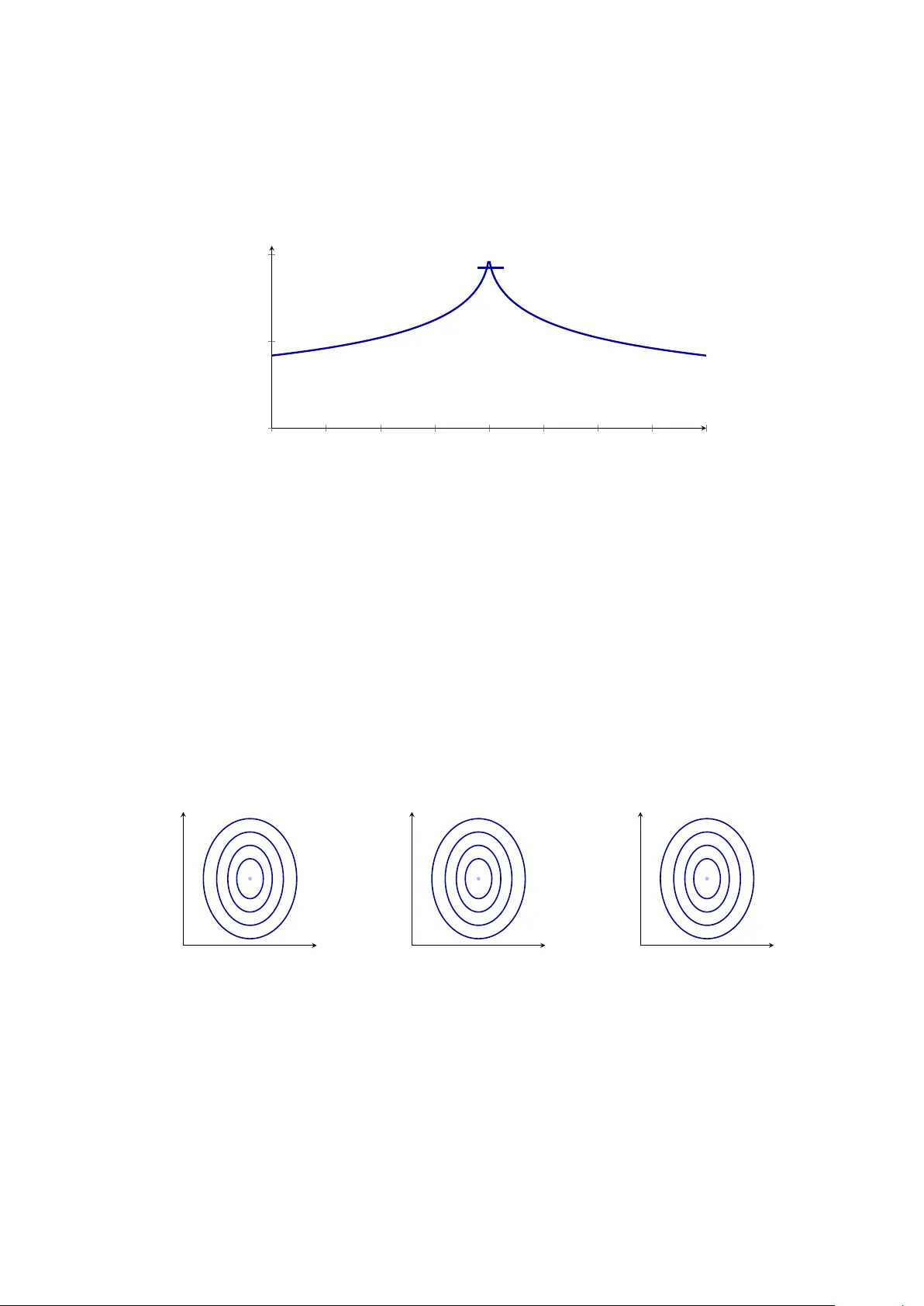
LOCAL ASYMPTOTIC NORMALITY F OR MIXED FRA CTIONAL ORNSTEIN–UHLENBECK PR OCESS UNDER HIGH-FREQUENCY OBSER V A TION Cai Ch unhao Departmen t of Mathematics, Sun Y at Sen Univ ersity caichh9@mail.sysu.edu.cn Shang Yiwu Sc ho ol of Mathematical Sciences, Nank ai Universit y shanyw@mail.nankai.edu.cn Zhang Cong Departmen t of Mathematics, Zhejiang Universit y zcong@zju.edu.cn Marc h 18, 2026 Abstract This pap er establishes a complete three parameter LAN framew ork for the mixed frac- tional Ornstein–Uhlen beck pro cess d X t = − αX t d t + d M H t , M H t = σ B H t + W t , under stationary initialization and discrete high-frequency observ ation of the Gaussian v ector X ( n ) = ( X k ∆ n ) ⊤ 1 ≤ k ≤ n , with ∆ n → 0 and T n = n ∆ n → ∞ , in the sup ercritical regime H > 3 / 4 . F ollo wing the pattern of the mixed fractional Brownian motion pap er [ 5 ], we first write the exact Gaussian score functions as centered quadratic forms, then isolate the explicit log ∆ n blo w-up term in the H -score, orthogonalize the H -remainder against the σ -score, and finally pro ject the α -score onto the orthogonal complement of the first t wo directions. This yields a non-diagonal low er-triangular rate matrix for the ra w score v ector and a diagonal LAN expansion for the pro jected central sequence. Each pro jected co ordinate liv es on the ( n ∆ n ) 1 / 2 scale, while the off-diagonal entries of the rate matrix enco de the asymptotic collinearity of the σ and H directions together with the residual correlation of the α direction. W e also include a figure design tailored to the three parameter setting, based on low frequency profile plots and pairwise Gaussian con tour plots of the pro jected limit. 1 In tro duction W e consider the mixed fractional Ornstein–Uhlenbeck (mfOU) process d X t = − αX t d t + d M H t , M H t = σ B H t + W t , t ≥ 0 , (1) where B H t is a fractional Brownian motion with Hurst index H ∈ (3 / 4 , 1) , W t is a standard Bro wnian motion indep enden t of B H t , with unknown parameter θ = ( σ, H , α ) . F or ∆ n → 0 , w e observ e the stationary Gaussian v ector X ( n ) = ( X ∆ n , X 2∆ n , . . . , X n ∆ n ) ⊤ , T n := n ∆ n → ∞ . 1 The mixed fractional Ornstein-Uhlen b ec k process incorp orates ideas from three different fields. First, the noise M H t = σ B H t + W t b elongs to the class of mixed Gaussian pro cesses. Mixed fractional Brownian motion w as introduced by Cheridito [ 8 ], who sho wed the phase transition at H = 3 / 4 . Cai et al. [ 6 ] developed a filtering-based canonical innov ation represen tation for mixed Gaussian pro cesses, which provides a general framew ork for likelihoo d analysis and change of measure argumen ts in mixed fractional mo dels. Second, for fractional Ornstein–Uhlenbeck and related fractional diffusion mo dels, statistical inference has been studied under both con tinuous and discrete observ ation sc hemes. Early lik eliho o d-based analysis for the fractional OU-t yp e mo del goes bac k to Kleptsyna and Le Breton [ 17 ]. F or parameter estimation in fOU mo dels, see also Hu and Nualart [ 14 ], Xiao et al. [ 19 ] in the particular regime of H , and Hu et al. [ 15 ] for estimation ov er general Hurst regimes. More recen tly , Shi et al. [ 18 ] studied the sp ectral densit y of discrete fOU pro cesses and prop osed an appro ximate Whittle maximum likelihoo d metho d. F or the mixed fractional OU mo del case, Chigansky and Kleptsyna [ 9 ] established consistency and asymptotic normalit y of the maxim um lik eliho o d estimator for the drift parameter, while Cai and Zhang [ 7 ] further inv estigated drift estimation and strong consistency of the MLE. Third, from the viewp oin t of asymptotic theory , high-frequency LAN theory for long-memory Gaussian models has developed rapidly in recent years. Brouste and F uk asa wa [ 4 ] prov ed the LAN prop ert y for fractional Gaussian noise under high-frequency observ ations with a non- diagonal rate matrix. More recently , Cai and Shang [ 5 ] obtained a LAN expansion for mixed fractional Bro wnian motion in the sup ercritical regime H > 3 / 4 . The present pap er extends this line of researc h to the stationary mfOU model with the full parameter v ector θ = ( σ, H , α ) under discrete high-frequency observ ation. Compared with the mixed fractional Brownian motion case, the additional mean-reversion parameter α creates a further non-orthogonal score direction, so that after removing the explicit σ log ∆ n term in the H -score one needs an additional pro jection to isolate the raw α -direction. Our aim is to establish a three parameter LAN expansion for the mfOU mo del, mirroring the pro of strategy in [ 5 ]. The main paper treats the sup ercritical regime H > 3 / 4 , b ecause in this range the low frequency singularity forces an additional asymptotic collinearity b et w een the σ -score and the H -score. One must therefore first remo ve the explicit σ log ∆ n con tribution from the raw H -score and then pro ject the remainder. In the mfOU model, a third parameter α is presen t, and after the first tw o directions hav e b een diagonalized a second pro jection is needed in order to isolate the raw α -direction. The lo wer regimes 1 / 2 < H < 3 / 4 and 0 < H < 1 / 2 are treated separately in the app endices at the level of complete score CL T s. The key phenomenon is the same as for mixed fractional Brownian motion in the sup ercritical regime H > 3 / 4 . Lo w frequencies dominate so strongly that the H -score contains a leading comp onen t asymptotically parallel to the σ -score. Hence a direct LAN statemen t in the raw co ordinates is badly conditioned. The cure is a t wo-step triangular diagonalization on the score side, follo wed b y a third pro jection for the α -direction. Notation. F or an in tegrable symbol g on [ − π , π ] , let T n ( g ) =  b g ( i − j )  1 ≤ i,j ≤ n , b g ( k ) = 1 2 π Z π − π g ( λ ) e − ikλ d λ. If Σ n ( θ ) is the co v ariance matrix of X ( n ) , w e write M i,n ( θ ) = Σ n ( θ ) − 1 / 2 ∂ i Σ n ( θ ) Σ n ( θ ) − 1 / 2 , i ∈ { σ, H , α } . Whenev er Z n ∼ N ( 0 , I n ) and A n is symmetric, we use the centered Gaussian quadratic form notation Q n ( A n ) := Z ⊤ n A n Z n − tr( A n ) . 2 The remainder of this paper pro ceeds as follows. In Section 2, w e state the main LAN theo- rem and introduce the k ey matrices and orthogonalization scheme that provide the foundation for the analysis. Section 3 recalls a fundamental CL T for cen tered Gaussian quadratic forms, whic h serv es as the main technical to ol throughout the pap er. In Section 4, we carry out a detailed asymptotic analysis of the three score functions, including the necessary pro jections that diagonalize the score v ector and yield the join t cen tral limit theorem. Section 5 completes the pro of of the LAN prop ert y via matrix expansions and T a ylor appro ximations. Section 6 outlines a figure design tailored to the three parameter setting, providing a visual interpreta- tion of the asymptotic results. Finally , sev eral app endices treat the remaining Hurst regimes 1 / 2 < H < 3 / 4 and 0 < H < 1 / 2 , establishing complete score CL T s and thereb y extending the scop e of the analysis. 2 Main Results Under stationary initialization, ( X k ∆ ) k ∈ Z is centered stationary Gaussian. The discrete sp ectral densit y of the sampled pro cess can b e written as f ∆ ( λ ; θ ) = f ( H ) ∆ ( λ ; α, σ, H ) + f ( W ) ∆ ( λ ; α ) , (2) with f ( H ) ∆ ( λ ) = σ 2 C ( H )∆ 2 H X k ∈ Z | λ + 2 π k | 1 − 2 H ( α ∆) 2 + ( λ + 2 π k ) 2 , C ( H ) := Γ(2 H + 1) sin( πH ) , (3) (see [ 16 ]) and f ( W ) ∆ ( λ ) = 1 − e − 2 α ∆ 2 α 1 1 + e − 2 α ∆ − 2 e − α ∆ cos λ . (4) Let Σ n ( θ ) := T n  f ∆ n ( · ; θ )  . Then the exact Gaussian log-likelihoo d is ℓ n ( θ ) = − 1 2  log de t Σ n ( θ ) + ( X ( n ) ) ⊤ Σ n ( θ ) − 1 X ( n )  + C , where C is a constant. If Z n := Σ n ( θ ) − 1 / 2 X ( n ) ∼ N (0 , I n ) , then eac h exact score comp onen t has the centered quadratic-form represen tation S i,n ( θ ) := ∂ i ℓ n ( θ ) = 1 2  Z ⊤ n M i,n ( θ ) Z n − tr( M i,n ( θ ))  , i ∈ { σ, H , α } . (5) This is the exact starting p oint of the whole argumen t. W e b egin with the exact Gaussian score represen tation and then state the LAN theorem. The pro ofs are p ostponed to later sections, in direct analogy with the organization of [ 5 ]. Theorem 2.1. Assume H ∈ (3 / 4 , 1) , σ > 0 , α > 0 , and ∆ n → 0 . F or the pr oje cte d sc or e CL Ts we imp ose log 2 n n ∆ n → 0 , (6) and for the final LAN r emainder c ontr ol we further assume the p olynomial mesh c ondition ∆ n = n − κ , 0 < κ < 1 . (7) 3 L et M n b e the lower-triangular sc or e tr ansformation define d in ( 28 ) , and let r n ( θ ) := p n ∆ n ( M ⊤ n ) − 1 . F or every fixe d h ∈ R 3 , set θ n,h = θ + r n ( θ ) − 1 h . Then ℓ n ( θ n,h ) − ℓ n ( θ ) = h ⊤ Ξ n − 1 2 h ⊤ I ⊥ ( θ ) h + o P θ (1) , wher e Ξ n = 1 √ n ∆ n    S σ,n R ⊥ H,n S ⊥ α,n    d − → N  0 , I ⊥ ( θ )  , I ⊥ ( θ ) = diag  I σ σ , I ⊥ H H , I ⊥ αα  . The definitions of the symb ols ar e: S σ,n in ( 8 ) , R ⊥ H,n in ( 15 ) and ( 16 ) , S ⊥ α,n in ( 24 ) , and I ⊥ ( θ ) with c omp onents I σ σ in ( 13 ) , I ⊥ H H in ( 20 ) , I ⊥ αα in ( 26 ) . Thus the exp eriment gener ate d by X ( n ) is lo c al ly asymptotic al ly normal at θ . Remark 2.2. The pro jected score CL T s prov ed using Sections 3–4 only require ( 6 ): after pro jection, the op erator norms of D ⊥ H,n and A ⊥ α,n are of order log n , while their F rob enius norms are of order ( n ∆ n ) 1 / 2 . The extra p olynomial-mesh assumption ( 7 ) is used only in Section 5, where w e strengthen the Hessian and third-order remainder b ounds enough to close the LAN pro of in the same st yle as [ 5 ]. 2.1 The three basic matrices In this subsection, w e introduce the three basic matrices C σ,n , D H,n and A α,n that constitute the core of the score functions for σ , H and α , resp ectiv ely , and serve as the foundation for the sub- sequen t asymptotic analysis and orthogonal pro jections. F or notational simplicity , throughout what follo ws we write Σ n ( θ ) as Σ n . Define h ∆ ( λ ) := ∂ σ f ∆ ( λ ) = 2 σ f ( H ) ∆ ( λ ) , C σ,n := Σ − 1 / 2 n T n ( h ∆ n )Σ − 1 / 2 n . Then S σ,n = 1 2 Q n ( C σ,n ) . (8) F or the H -direction, set S H, ∆ ( λ ) := X k ∈ Z | λ + 2 π k | 1 − 2 H ( α ∆) 2 + ( λ + 2 π k ) 2 . A direct differentiation of ( 3 ) giv es ∂ H f ∆ ( λ ) = f ( H ) ∆ ( λ )  2 log ∆ + ∂ H log C ( H ) + ∂ H log S H, ∆ ( λ )  . Since σ log ∆ ∂ σ f ∆ = 2 log ∆ f ( H ) ∆ , w e obtain the exact decomp osition ∂ H f ∆ ( λ ) = σ log ∆ ∂ σ f ∆ ( λ ) + r ∆ ( λ ) , (9) where r ∆ ( λ ) := f ( H ) ∆ ( λ )  ∂ H log C ( H ) + ∂ H log S H, ∆ ( λ )  . Define D H,n := Σ − 1 / 2 n T n ( r ∆ n )Σ − 1 / 2 n . 4 Then S H,n = σ log ∆ n S σ,n + R H,n , R H,n := 1 2 Q n ( D H,n ) . (10) Finally define the raw α -matrix A α,n := Σ − 1 / 2 n T n ( ∂ α f ∆ n )Σ − 1 / 2 n , so that S α,n = 1 2 Q n ( A α,n ) . (11) 3 Preliminaries: A CL T for Gaussian quadratic forms In this section we collect a fundamental to ol for the analysis of centered Gaussian quadratic forms, which is imp ortant for all subsequen t score-CL T pro ofs. Lemma 3.1 states that a quadratic form of indep enden t standard normal v ariables is asymptotically normal if the ratio of its op er- ator norm to its F rob enius norm tends to zero. This condition will b e verified rep eatedly for the matrices C σ,n , D H,n , A α,n and their pro jected versions, allo wing us to deduce the asymptotic distribution of the exact score comp onents derived in the previous section. Lemma 3.1. L et Z n ∼ N (0 , I n ) and let M n b e r e al symmetric matric es. If ∥ M n ∥ op ∥ M n ∥ F → 0 , then Q n ( M n ) √ 2 ∥ M n ∥ F d − → N (0 , 1) . Equivalently, if ∥ M n ∥ 2 op / tr( M 2 n ) → 0 , then Q n ( M n ) p 2tr( M 2 n ) d − → N (0 , 1) . Pr o of. See [ 5 ]. Remark 3.2. Let Q n ( M n ) := Z ⊤ n M n Z n − tr( M n ) b e a cen tered Gaussian quadratic form with M n real symmetric, and let λ 1 ,n , . . . , λ n,n denote the eigenv alues of M n . Then w e obtain V ar( Q n ( M n )) = 2 n X j =1 λ 2 j,n = 2tr( M 2 n ) = 2 ∥ M n ∥ 2 F . (12) Remark 3.3. The asymptotic v ariances of all subsequent score comp onen ts S σ,n , R H,n and S α,n are deriv ed from equation ( 12 ) through tr( C 2 σ,n ) , tr( D 2 H,n ) and tr( A 2 α,n ) , resp ectiv ely . 4 Analysis of the score functions In this section w e analyze the three exact score directions introduced in Section 2 and establish the pro jected score central limit theorems needed for the LAN expansion. W e follow the orthogo- nalization scheme: first, we analyze the σ -score. Next, w e remo ve the logarithmic term from the H -score and pro ject the remainder. Finally , we pro ject the α -score to obtain the diagonalized cen tral sequence. 5 4.1 The σ -direction of the score functions W e b egin with the σ -direction, which pro vides the basis for the whole argumen t. In this sub- section we iden tify the asymptotic Fisher information in the σ -co ordinate and pro ve the central limit theorem for S σ,n on √ n ∆ n scale. First, w e introduce the ratio sym b ol g σ,n ( λ ) := ∂ σ f ∆ n ( λ ) f ∆ n ( λ ) = h ∆ n ( λ ) f ∆ n ( λ ) = 2 σ f ( H ) ∆ n ( λ ) f ∆ n ( λ ) ∈ h 0 , 2 σ i . Lemma 4.1. F or al l n , ∥ C σ,n ∥ op ≤ 2 σ . Pr o of. By the generalized Ra yleigh quotien t for the pair  T n ( h ∆ n ) , Σ n ( θ )  (see remark 4.2 ), together with the T o eplitz quadratic-form represen tation, we obtain ∥ C σ,n ∥ op = sup x  =0 x ⊤ T n ( h ∆ n ) x x ⊤ T n ( f ∆ n ) x ≤ sup λ ∈ [ − π ,π ] h ∆ n ( λ ) f ∆ n ( λ ) ≤ 2 σ . Remark 4.2. Let A n b e a real symmetric matrix and let Σ n b e symmetric positive definite. Then for every x ∈ R n \ { 0 } , x ⊤ A n x x ⊤ Σ n x is the generalized Rayleigh quotien t asso ciated with the pair  A n , Σ n  . Equiv alently , setting y = Σ 1 / 2 n x , one obtains x ⊤ A n x x ⊤ Σ n x = y ⊤ Σ − 1 / 2 n A n Σ − 1 / 2 n y y ⊤ y . Therefore sup x  =0     x ⊤ A n x x ⊤ Σ n x     =   Σ − 1 / 2 n A n Σ − 1 / 2 n   op . Lemma 4.3. Assume ∆ n → 0 and T n = n ∆ n → ∞ . Then tr( C 2 σ,n ) = n 2 π Z π − π g σ,n ( λ ) 2 d λ + o ( n ∆ n ) . Pr o of. Set B n := Σ − 1 n T n ( h ∆ n ) . Since C σ,n is similar to B n , one has tr( C 2 σ,n ) = tr( B 2 n ) = tr  Σ − 1 n T n ( h ∆ n )Σ − 1 n T n ( h ∆ n )  . Let G n := T n ( g σ,n ) and R n := B n − G n . The same lo w frequency truncation and T o eplitz- pro duct argument as in the mfBm pro of [ 5 ] gives ∥ R n ∥ op = o (1) , ∥ R n ∥ F = o (( n ∆ n ) 1 / 2 ) . Therefore tr( B 2 n ) = tr( G 2 n ) + 2tr( G n R n ) + tr( R 2 n ) = tr( G 2 n ) + o ( n ∆ n ) , b ecause ∥ G n ∥ op ≤ sup λ | g σ,n ( λ ) | ≤ 2 /σ . Finally , for g ∈ L 2 ([ − π , π ]) the F ejér-k ernel identit y yields tr( T n ( g ) 2 ) = n 2 π Z π − π g ( λ ) 2 F n ( λ ) d λ, 6 where F n is the F ejér k ernel. Applying this with g = g σ,n and using that the transition region of g σ,n is concen trated on the region | λ | ≍ ∆ n giv es tr( G 2 n ) = n 2 π Z π − π g σ,n ( λ ) 2 d λ + o ( n ∆ n ) . Com bining the tw o displays prov es the claim. Set ρ := 2 H − 1 ∈ (1 / 2 , 1) , A := σ 2 Γ(2 H + 1) sin( π H ) . where Γ( · ) denotes the Gamma function. Then on the lo w frequency region λ = ∆ n u , one has f ( H ) ∆ n (∆ n u ) f ( W ) ∆ n (∆ n u ) ≈ A | u | − ρ , w ( u ) := 1 1 + A − 1 | u | ρ . Hence g σ,n (∆ n u ) → (2 /σ ) w ( u ) . Lemma 4.4. Assume H > 3 / 4 . Then Z π − π g σ,n ( λ ) 2 d λ ∼ ∆ n 8 σ 2 ρ A 1 /ρ Γ  1 ρ  Γ  2 − 1 ρ  . Conse quently, tr( C 2 σ,n ) ∼ 2( n ∆ n ) I σ σ ( σ, H ) , wher e I σ σ ( σ, H ) = 2 π σ 2 (2 H − 1)  σ 2 Γ(2 H + 1) sin( π H )  1 / (2 H − 1) Γ  1 2 H − 1  Γ  2 − 1 2 H − 1  . (13) Pr o of. W rite g σ,n ( λ ) = (2 /σ ) w ∆ n ( λ ) with w ∆ ( λ ) := f ( H ) ∆ ( λ ) f ( H ) ∆ ( λ ) + f ( W ) ∆ ( λ ) . The contribution to w 2 ∆ n ( λ ) is concentrated on the region | λ | ≍ ∆ n . On that region the OU denominator (( α ∆ n ) 2 + λ 2 ) − 1 is common to b oth sp ectral pieces and cancels in the ratio, so for λ = ∆ n u , f ( H ) ∆ n (∆ n u ) f ( W ) ∆ n (∆ n u ) → A | u | − ρ , w ∆ n (∆ n u ) → w ( u ) := 1 1 + A − 1 | u | ρ . Since ρ > 1 / 2 , the function w ( u ) 2 is in tegrable on R , and dominated conv ergence giv es Z π − π g σ,n ( λ ) 2 d λ ∼ ∆ n 4 σ 2 Z R w ( u ) 2 d u. Using t = | u | ρ / A , Z R w ( u ) 2 d u = 2 ρ A 1 /ρ Z ∞ 0 t 1 /ρ − 1 (1 + t ) 2 d t = 2 ρ A 1 /ρ Γ  1 ρ  Γ  2 − 1 ρ  , whic h pro ves the display ed asymptotic. The form ula for tr( C 2 σ,n ) then follo ws from lemma 4.3 . Prop osition 4.5. Under H > 3 / 4 , ∆ n → 0 and T n = n ∆ n → ∞ , S σ,n √ n ∆ n d − → N  0 , I σ σ ( σ, H )  . 7 Pr o of. By lemmas 4.1 , 4.3 and 4.4 , ∥ C σ,n ∥ 2 op tr( C 2 σ,n ) ≲ 1 n ∆ n → 0 . Apply lemma 3.1 to C σ,n and use ( 8 ). 4.2 The H -direction of the score functions: remo ving the explicit logarithmic term W e next turn to the H -score. The key p oin t is that its raw form contains the explicit singular term σ log ∆ n S σ,n , so here we isolate the remainder R H,n and analyze its asymptotic property . Set L n := log(1 / ∆ n ) , g H,n ( λ ) := r ∆ n ( λ ) f ∆ n ( λ ) = w ∆ n ( λ ) ψ ∆ n ( λ ) , where w ∆ ( λ ) := f ( H ) ∆ ( λ ) f ∆ ( λ ) ∈ [0 , 1] , ψ ∆ ( λ ) := ∂ H log C ( H ) + ∂ H log S H, ∆ ( λ ) . On the scale λ = ∆ n u one has ψ ∆ n (∆ n u ) = 2 L n − 2 log | u | + ∂ H log C ( H ) + O (1) . Hence the raw remainder has one logarithm more than the σ -direction. Lemma 4.6. Under H > 3 / 4 and T n → ∞ , ∥ D H,n ∥ op ≲ L n + log n. In p articular, for p ower meshes ∆ n = n − κ , ∥ D H,n ∥ op = O (log n ) . Pr o of. By remark 4.2 , ∥ D H,n ∥ op = sup x  =0 | x ⊤ T n ( r ∆ n ) x | x ⊤ T n ( f ∆ n ) x ≤ sup λ ∈ [ − π ,π ] | g H,n ( λ ) | . On the low frequency scale λ = ∆ n u one has ψ ∆ n (∆ n u ) = 2 L n − 2 log | u | + O (1) . In a size- n T o eplitz quadratic form, frequencies b elo w order 1 /n are not resolved, so on the effectiv e range | u | = | λ | / ∆ n ≳ ( n ∆ n ) − 1 w e hav e | log | u || ≲ L n + log n . Since 0 ≤ w ∆ n ≤ 1 , it follo ws that | g H,n ( λ ) | = | w ∆ n ( λ ) ψ ∆ n ( λ ) | ≲ L n + log n, whic h yields the claim. Lemma 4.7. Under H > 3 / 4 and T n → ∞ , tr( D 2 H,n ) = n 2 π Z π − π g H,n ( λ ) 2 d λ + o ( n ∆ n L 2 n ) , and mor e over tr( D 2 H,n ) ∼ 2( n ∆ n L 2 n ) I rem H H ( σ, H ) , with I rem H H ( σ, H ) = 1 π J 0 , J 0 := Z R d u (1 + A − 1 | u | ρ ) 2 = 2 ρ A 1 /ρ Γ  1 ρ  Γ  2 − 1 ρ  . (14) 8 Pr o of. Let B n := Σ − 1 n T n ( r ∆ n ) . Since D H,n is similar to B n , tr( D 2 H,n ) = tr( B 2 n ) = tr  Σ − 1 n T n ( r ∆ n )Σ − 1 n T n ( r ∆ n )  . With G n := T n ( g H,n ) and R n := B n − G n , the same sandwic h approximation as in lemma 4.3 yields ∥ R n ∥ op = o ( L n ) , ∥ R n ∥ F = o (( n ∆ n ) 1 / 2 L n ) , so that tr( D 2 H,n ) = tr( G 2 n ) + o ( n ∆ n L 2 n ) . The F ejér-kernel trace iden tity then giv es the displa yed in tegral approximation. F or the main term, write λ = ∆ n u . Since w ∆ n (∆ n u ) → w ( u ) and ψ ∆ n (∆ n u ) = 2 L n + ∂ H log C ( H ) − 2 log | u | + O (1) , w e obtain g H,n (∆ n u ) = w ( u )  2 L n + O (1) − 2 log | u |  + o (1) . Because ρ > 1 / 2 , dominated con vergence gives Z π − π g H,n ( λ ) 2 d λ ∼ 4∆ n L 2 n Z R w ( u ) 2 d u = 4∆ n L 2 n J 0 . Com bining this with the trace approx imation pro ves the result. Prop osition 4.8. Under H > 3 / 4 and T n → ∞ , R H,n √ n ∆ n L n d − → N  0 , I rem H H ( σ, H )  . Pr o of. By lemma 4.6 and lemma 4.7 ∥ D H,n ∥ op ∥ D H,n ∥ F ≲ L n + log n √ n ∆ n L n → 0 , Applying lemma 3.1 to D H,n completes the pro of. 4.3 Pro jection of the H -remainder against the σ -direction Because R H,n still contains the comp onen t asymptotically parallel to S σ,n , we pro ject it out. Define a n := tr( C σ,n D H,n ) tr( C 2 σ,n ) , D ⊥ H,n := D H,n − a n C σ,n , R ⊥ H,n := 1 2 Q n ( D ⊥ H,n ) . (15) Then R H,n = a n S σ,n + R ⊥ H,n and S H,n = β n ( θ ) S σ,n + R ⊥ H,n , β n ( θ ) := σ log ∆ n + a n . (16) Lemma 4.9. Under H > 3 / 4 and T n → ∞ , tr( C σ,n D H,n ) = n 2 π Z π − π g σ,n ( λ ) g H,n ( λ ) d λ + o ( n ∆ n L n ) , with tr( C σ,n D H,n ) ∼ ( n ∆ n L n ) 2 π σ J 0 . Mor e over, a n = σ  L n + 1 2 b − m  + o (1) , (17) wher e b := ∂ H log C ( H ) = 2Ψ(2 H + 1) + π cot( π H ) , m := 1 ρ  log A + Ψ(1 /ρ ) − Ψ(2 − 1 /ρ )  . (18) Her e Ψ denotes the digamma function and J 0 define d in ( 14 ) . 9 Pr o of. W e first reduce the trace of the pro duct of matrices to a trace in volving only T o eplitz matrices generated by symbol ratios. Since C σ,n = Σ − 1 / 2 n T n ( h ∆ n )Σ − 1 / 2 n , D H,n = Σ − 1 / 2 n T n ( r ∆ n )Σ − 1 / 2 n , the cyclicit y of the trace yields tr( C σ,n D H,n ) = tr  Σ − 1 n T n ( h ∆ n )Σ − 1 n T n ( r ∆ n )  . W riting g σ,n ( λ ) := h ∆ n ( λ ) f ∆ n ( λ ) , g H,n ( λ ) := r ∆ n ( λ ) f ∆ n ( λ ) , and letting G σ,n := T n ( g σ,n ) , G H,n := T n ( g H,n ) , the same T o eplitz sandwich appro ximation as in the previous sections gives tr( C σ,n D H,n ) = tr( G σ,n G H,n ) + o ( n ∆ n L n ) . W e then pass from the matrix trace to the corresp onding sp ectral integral. By the standard T o eplitz trace identit y , tr( G σ,n G H,n ) = n 2 π Z π − π g σ,n ( λ ) g H,n ( λ ) d λ + o ( n ∆ n L n ) , and therefore tr( C σ,n D H,n ) = n 2 π Z π − π g σ,n ( λ ) g H,n ( λ ) d λ + o ( n ∆ n L n ) . It remains to ev aluate this in tegral on the lo w frequency scale. Put λ = ∆ n u . Using the lo w frequency expansions established earlier, we ha ve uniformly on compact u -sets, g σ,n (∆ n u ) → 2 σ w ( u ) , g H,n (∆ n u ) = w ( u )  2 L n + b − 2 log | u |  + o (1) , where w ( u ) = 1 1 + A − 1 | u | ρ . Moreo ver, after separating the explicit leading L n -term, the remaining part is dominated by a m ultiple of w ( u ) 2 (1 + | log | u || ) , whic h is integrable b ecause ρ > 1 / 2 . Hence dominated conv er- gence applies to the constan t-order term, while the leading logarithmic contribution is carried b y J 0 . Therefore g σ,n (∆ n u ) g H,n (∆ n u ) = 2 σ w ( u ) 2  2 L n + b − 2 log | u |  + o (1) , and consequen tly Z π − π g σ,n ( λ ) g H,n ( λ ) d λ = ∆ n  4 σ L n J 0 + 2 σ ( bJ 0 − 2 J 1 )  + o (∆ n ) , where J 0 := Z R 1 (1 + A − 1 | u | ρ ) 2 d u, J 1 := Z R log | u | (1 + A − 1 | u | ρ ) 2 d u. This pro ves the asymptotic relation tr( C σ,n D H,n ) ∼ ( n ∆ n L n ) 2 π σ J 0 . 10 Finally , by dividing the preceding expansion by the corresp onding one for tr( C 2 σ,n ) , w e obtain a n = σ  L n + 1 2 b − J 1 J 0  + o (1) . It only remains to identify the ratio J 1 /J 0 . By the c hange of v ariables t = | u | ρ / A , J 1 J 0 = 1 ρ  log A + Ψ(1 /ρ ) − Ψ(2 − 1 /ρ )  =: m. Therefore a n = σ  L n + 1 2 b − m  + o (1) , whic h is exactly ( 17 ). The expression for b in ( 18 ) is just b = ∂ H log C ( H ) = 2Ψ(2 H + 1) + π cot( π H ) . The pro of is complete. Lemma 4.10. F or every n , tr( C σ,n D ⊥ H,n ) = 0 , Co v ( S σ,n , R ⊥ H,n ) = 0 . Pr o of. The trace iden tit y is immediate from ( 15 ). Since centered Gaussian quadratic forms satisfy Co v  1 2 Q n ( A ) , 1 2 Q n ( B )  = 1 2 tr( AB ) , w e obtain the co v ariance statemen t. Lemma 4.11. Assume the mild str engthening log 2 n n ∆ n → 0 . (19) Then    D ⊥ H,n    op = O (log n ) , tr  ( D ⊥ H,n ) 2  ∼ 2( n ∆ n ) I ⊥ H H ( σ, H ) , wher e I ⊥ H H ( σ, H ) = 1 π  J 2 − J 2 1 J 0  , J 2 := Z R (log | u | ) 2 (1 + A − 1 | u | ρ ) 2 d u. (20) Equivalently, I ⊥ H H ( σ, H ) = J 0 π ρ 2  Ψ 1 (1 /ρ ) + Ψ 1 (2 − 1 /ρ )  , (21) with Ψ 1 the trigamma function and J 0 in ( 14 ) . Pr o of. Set e g n ( λ ) := g H,n ( λ ) − a n g σ,n ( λ ) . Since D ⊥ H,n = D H,n − a n C σ,n , the Ra yleigh-quotient argumen t used for D H,n giv es    D ⊥ H,n    op ≤ sup λ | e g n ( λ ) | . Using lemma 4.9 , for λ = ∆ n u one has e g n (∆ n u ) = w ( u )  − 2 log | u | + 2 m + o (1)  , so the leading 2 L n + b terms cancel. T o b ound the remaining profile, recall that frequencies b elo w order 1 /n are not resolved in a size- n T o eplitz form. Hence on the effective low frequency region | u | = | λ | / ∆ n ≳ ( n ∆ n ) − 1 , 11 w e ha ve | log | u || ≲ L n + log n . Since 0 ≤ w ( u ) ≤ 1 and the centered combination eliminates the L n con tribution, this gives sup λ ∈ [ − π ,π ] | e g n ( λ ) | ≤ C (1 + log n ) , and therefore    D ⊥ H,n    op = O (log n ) . F or the trace, expand tr(( D ⊥ H,n ) 2 ) = tr( D 2 H,n ) − 2 a n tr( C σ,n D H,n ) + a 2 n tr( C 2 σ,n ) . Insert the asymptotics from lemmas 4.4 , 4.7 and 4.9 . After dividing by n ∆ n , the L 2 n and L n con tributions cancel exactly , and only the centered logarithmic term remains. Equiv alen tly , the T o eplitz sandwich reduction applied directly to D ⊥ H,n yields tr(( D ⊥ H,n ) 2 ) = n 2 π Z π − π e g n ( λ ) 2 d λ + o ( n ∆ n ) . P assing to the scale λ = ∆ n u and using the limit ab ov e giv es Z π − π e g n ( λ ) 2 d λ ∼ 4∆ n Z R w ( u ) 2 (log | u | − m ) 2 d u = 4∆ n  J 2 − J 2 1 J 0  . This prov es ( 20 ). The trigamma form follo ws by differen tiating the b eta-function expression for J 0 t wice with resp ect to 1 /ρ . Prop osition 4.12. Assume ( 19 ) . Then R ⊥ H,n √ n ∆ n d − → N  0 , I ⊥ H H ( σ, H )  . Pr o of. By lemma 4.11 ,    D ⊥ H,n    op    D ⊥ H,n    F ≲ log n √ n ∆ n → 0 . The prop osition follo ws from lemma 3.1 . 4.4 The α -direction of the score functions and the second pro jection W e then analyze the α -score. Although this direction has no logarithmic blow-up, it still carries non trivial correlations, so w e in tro duce a second pro jection, iden tify the corresponding Sch ur- complemen t information, and pro ve the CL T for the pro jected score S ⊥ α,n . The α -score has no logarithmic explosion. Define g α,n ( λ ) := ∂ α f ∆ n ( λ ) f ∆ n ( λ ) . On the scale λ = ∆ n u , the common OU denominator contributes the main α -dep endence, hence g α,n (∆ n u ) = − 2 α α 2 + u 2 + o (1) . This giv es the same order n ∆ n as in the pro jected H -direction. 12 Lemma 4.13. Under H > 3 / 4 and T n → ∞ , ∥ A α,n ∥ op = O (1) , tr( A 2 α,n ) = n 2 π Z π − π g α,n ( λ ) 2 d λ + o ( n ∆ n ) , and tr( A 2 α,n ) ∼ n ∆ n α . Conse quently, I αα ( α ) = 1 2 α , S α,n √ n ∆ n d − → N  0 , 1 2 α  . (22) Pr o of. W e first pro ve the op erator b ound by writing A α,n through the corresp onding generalized Ra yleigh quotient. By remark 4.2 , ∥ A α,n ∥ op = sup y  =0 | y ⊤ T n ( ∂ α f ∆ n ) y | y ⊤ T n ( f ∆ n ) y ≤ sup λ ∈ [ − π ,π ]     ∂ α f ∆ n ( λ ) f ∆ n ( λ )     = sup λ ∈ [ − π ,π ] | g α,n ( λ ) | . Because differentiation in α acts only on the OU filter, the low frequency denominator ( α ∆ n ) 2 + λ 2 is differen tiated into a b ounded rational factor. Hence sup λ ∈ [ − π ,π ] | g α,n ( λ ) | ≤ C , so that ∥ A α,n ∥ op = O (1) . W e next turn to the trace. By the same T o eplitz sandwich reduction used earlier in the pap er, one obtains tr( A 2 α,n ) = tr  T n ( g α,n ) 2  + o ( n ∆ n ) . Since g α,n is uniformly b ounded and lo calized on the scale | λ | ≍ ∆ n , the F ejér-kernel identit y giv es tr  T n ( g α,n ) 2  = n 2 π Z π − π g α,n ( λ ) 2 d λ + o ( n ∆ n ) , see [ 2 , 3 , 12 ] and therefore tr( A 2 α,n ) = n 2 π Z π − π g α,n ( λ ) 2 d λ + o ( n ∆ n ) . It remains to ev aluate the integral asymptotically . Put λ = ∆ n u , one has g α,n (∆ n u ) = − 2 α α 2 + u 2 + o (1) , whereas the contribution from | λ | ≫ ∆ n is negligible. Consequen tly , Z π − π g α,n ( λ ) 2 d λ ∼ ∆ n Z R 4 α 2 ( α 2 + u 2 ) 2 d u = ∆ n · 2 π α , whic h yields tr( A 2 α,n ) ∼ n ∆ n α . Finally , since ∥ A α,n ∥ op = O (1) , ∥ A α,n ∥ 2 F = tr( A 2 α,n ) ≍ n ∆ n → ∞ , w e hav e ∥ A α,n ∥ op ∥ A α,n ∥ F → 0 . 13 Applying lemma 3.1 to the centered quadratic form asso ciated with A α,n , w e obtain S α,n √ n ∆ n d − → N  0 , 1 2 α  . Equiv alently , I αα ( α ) = 1 2 α , whic h is exactly ( 22 ). The p oin t, how ev er, is not the raw CL T but the diagonalized one. Because S α,n still correlates with ( S σ,n , R ⊥ H,n ) , w e pro ject again. Define b σ,n := tr( A α,n C σ,n ) tr( C 2 σ,n ) , b H,n := tr( A α,n D ⊥ H,n ) tr(( D ⊥ H,n ) 2 ) , (23) and A ⊥ α,n := A α,n − b σ,n C σ,n − b H,n D ⊥ H,n , S ⊥ α,n := 1 2 Q n ( A ⊥ α,n ) . (24) Lemma 4.14. F or every n , tr( A ⊥ α,n C σ,n ) = 0 , tr( A ⊥ α,n D ⊥ H,n ) = 0 . Ther efor e, Co v ( S ⊥ α,n , S σ,n ) = 0 , Co v ( S ⊥ α,n , R ⊥ H,n ) = 0 . Pr o of. Using ( 24 ) and the already prov ed identit y tr( C σ,n D ⊥ H,n ) = 0 from lemma 4.10 , we obtain tr( A ⊥ α,n C σ,n ) = tr( A α,n C σ,n ) − b σ,n tr( C 2 σ,n ) − b H,n tr( D ⊥ H,n C σ,n ) = 0 , b ecause b σ,n = tr( A α,n C σ,n ) / tr( C 2 σ,n ) . Similarly , tr( A ⊥ α,n D ⊥ H,n ) = tr( A α,n D ⊥ H,n ) − b H,n tr(( D ⊥ H,n ) 2 ) − b σ,n tr( C σ,n D ⊥ H,n ) = 0 . The co v ariance identities follow from Co v  1 2 Q n ( A ) , 1 2 Q n ( B )  = 1 2 tr( AB ) for cen tered Gaussian quadratic forms. Lemma 4.15. Assume ( 19 ) . Then b σ,n = O (1) and b H,n = O (1) , tr  ( A ⊥ α,n ) 2  = tr( A 2 α,n ) − tr( A α,n C σ,n ) 2 tr( C 2 σ,n ) − tr( A α,n D ⊥ H,n ) 2 tr(( D ⊥ H,n ) 2 ) , (25) and    A ⊥ α,n    op = O (log n ) , tr  ( A ⊥ α,n ) 2  ≍ n ∆ n . Henc e tr  ( A ⊥ α,n ) 2  ∼ 2( n ∆ n ) I ⊥ αα ( α, σ, H ) , with I ⊥ αα given by ( 26 ) . 14 Pr o of. The relev an t mixed traces all liv e on the same lo w frequency scale | λ | ≍ ∆ n . More precisely , if e g n ( λ ) := g H,n ( λ ) − a n g σ,n ( λ ) , then the same similarity reduction and T o eplitz sandwich argument as in Sections 3–4 gives tr( A α,n C σ,n ) = n 2 π Z π − π g α,n ( λ ) g σ,n ( λ ) d λ + o ( n ∆ n ) , tr( A α,n D ⊥ H,n ) = n 2 π Z π − π g α,n ( λ ) e g n ( λ ) d λ + o ( n ∆ n ) . On the region λ = ∆ n u one has g α,n (∆ n u ) → q α ( u ) := − 2 α α 2 + u 2 , g σ,n (∆ n u ) → 2 σ w ( u ) , e g n (∆ n u ) → − 2 w ( u )(log | u | − m ) . while outside that region the contribution is negligible. Since all three limiting profiles are square- in tegrable against each other, the normalized mixed traces hav e finite limits. In particular, tr( A 2 α,n ) , tr( C 2 σ,n ) , tr(( D ⊥ H,n ) 2 ) , tr( A α,n C σ,n ) , tr( A α,n D ⊥ H,n ) = O ( n ∆ n ) , and therefore b σ,n = O (1) and b H,n = O (1) . Expanding the square in ( 24 ) and using lemmas 4.10 and 4.14 giv es the exact identit y ( 25 ). Dividing by 2 n ∆ n yields the Sc hur-complemen t constan t ( 26 ). Since A ⊥ α,n is the Hilbert–Schmidt residual after orthogonal pro jection of A α,n on to span { C σ,n , D ⊥ H,n } , the right-hand side of ( 25 ) is nonnegative for every n . In the limit it is strictly p ositive because the profile q α ( u ) is not con tained in the span of w ( u ) and w ( u )(log | u | − m ) . F or the op erator norm, com bine lemmas 4.13 , 4.1 and 4.11 with the b oundedness of b σ,n and b H,n :    A ⊥ α,n    op ≤ ∥ A α,n ∥ op + | b σ,n | ∥ C σ,n ∥ op + | b H,n |    D ⊥ H,n    op = O (1) + O (1) + O (log n ) = O (log n ) . This pro ves the lemma. Remark 4.16. The pro jected constan t is naturally identified through the Sc hur-complemen t form ula I ⊥ αα := I αα − I 2 ασ I σ σ − ( I ⊥ αH ) 2 I ⊥ H H , (26) where I ασ := lim n →∞ 1 2 n ∆ n tr( A α,n C σ,n ) , I ⊥ αH := lim n →∞ 1 2 n ∆ n tr( A α,n D ⊥ H,n ) . (27) This is exactly the three dimensional analogue of the tw o-parameter orthogonalization in the [ 5 ]. The pro jected information is the raw α -information minus the tw o squared pro jections onto the already diagonalized ( σ, H ⊥ ) directions. Prop osition 4.17. Assume ( 19 ) . Then S ⊥ α,n √ n ∆ n d − → N  0 , I ⊥ αα ( α, σ, H )  . Pr o of. By lemma 4.15 ,   A ⊥ α,n   op   A ⊥ α,n   F ≲ log n √ n ∆ n → 0 . The prop osition follo ws from lemma 3.1 . 15 4.5 Join t diagonalized central sequence Finally , w e collect the three orthogonalized score comp onen ts ( S σ,n , R ⊥ H,n , S ⊥ α,n ) ⊤ in to a single cen tral sequence. The purp ose of this subsection is to combine the previous one dimensional limits and exact orthogonalit y relations into a joint Gaussian limit with diagonal cov ariance. Collect the three diagonalized directions: Ξ n := 1 √ n ∆ n     S σ,n R ⊥ H,n S ⊥ α,n     . Prop osition 4.18. Assume ( 19 ) . Then Ξ n d − → N  0 , I ⊥ ( θ )  , I ⊥ ( θ ) := diag  I σ σ , I ⊥ H H , I ⊥ αα  . Pr o of. F or fixed ( u, v , w ) ∈ R 3 consider A n ( u, v , w ) := uC σ,n + v D ⊥ H,n + w A ⊥ α,n . By lemmas 4.10 and 4.14 , all cross traces v anish exactly , so tr( A n ( u, v , w ) 2 ) = u 2 tr( C 2 σ,n ) + v 2 tr(( D ⊥ H,n ) 2 ) + w 2 tr(( A ⊥ α,n ) 2 ) . Also, ∥ A n ( u, v , w ) ∥ op = O (log n ) , ∥ A n ( u, v , w ) ∥ 2 F ≍ n ∆ n . Hence ∥ A n ( u, v , w ) ∥ op / ∥ A n ( u, v , w ) ∥ F → 0 , and lemma 3.1 plus Cramér–W old finishes the pro of. W e no w summarize this section. Starting from the ra w score v ector ( S σ,n , S H,n , S α,n ) , w e first remo ve from S H,n its explicit log ∆ n part and its asymptotically collinear part in the σ -direction, whic h yields the residual term R ⊥ H,n . W e then pro ject the α -score onto the orthogonal comple- men t of the first tw o directions and obtain S ⊥ α,n . Thus the original score vector is transformed in to ( S σ,n , R ⊥ H,n , S ⊥ α,n ) , whose comp onents corresp ond to the three asymptotically separated di- rections in the LAN expansion. The rest of this section establishes their join t cen tral limit theorem and the asso ciated Gaussian central sequence. 5 The LAN prop ert y in high-frequency observ ation via matrix expansions The exact score-level triangularization is the cen tral structural identit y . First, S H,n = β n ( θ ) S σ,n + R ⊥ H,n , β n ( θ ) = σ log ∆ n + a n . Second, S α,n = b σ,n S σ,n + b H,n R ⊥ H,n + S ⊥ α,n . Therefore, with the raw score v ector ∇ ℓ n ( θ ) =  S σ,n , S H,n , S α,n  ⊤ , one has the exact low er-triangular score transformation M n ∇ ℓ n ( θ ) =    S σ,n R ⊥ H,n S ⊥ α,n    , M n := M (3) n M (2) n M (1) n , (28) 16 where M (1) n =   1 0 0 − σ log ∆ n 1 0 0 0 1   , M (2) n =   1 0 0 − a n 1 0 0 0 1   , M (3) n =   1 0 0 0 1 0 − b σ,n − b H,n 1   . Equiv alently , r n ( θ ) := p n ∆ n ( M ⊤ n ) − 1 , r n ( θ ) −⊤ = 1 √ n ∆ n M n . (29) This is the natural non-diagonal rate matrix in the original co ordinates. It is built from the successiv e remov al of the log ∆ n term, the orthogonal pro jection in the H -direction, and the final pro jection in the α -direction. 5.1 Matrix expansion of the likelihoo d ratio Fix h ∈ R 3 and set θ n,h := θ + r n ( θ ) − 1 h. W rite Σ n for the cov ariance matrix of X ( n ) and define the p erturbation matrix S n ( h ) := Σ n ( θ ) − 1 / 2  Σ n ( θ n,h ) − Σ n ( θ )  Σ n ( θ ) − 1 / 2 . Then, with Z n = Σ n ( θ ) − 1 / 2 X ( n ) ∼ N (0 , I n ) , ℓ n ( θ n,h ) − ℓ n ( θ ) = − 1 2 log det( I n + S n ( h )) − 1 2 Z ⊤ n  ( I n + S n ( h )) − 1 − I n  Z n . (30) W e use tw o standard matrix T aylor lemmas. They provide the required expansions for the matrix logarithm and matrix inv erse. Lemma 5.1. If matrix S is symmetric and ∥ S ∥ op ≤ 1 / 2 , then log det( I + S ) = tr( S ) − 1 2 tr( S 2 ) + R log ( S ) , | R log ( S ) | ≤ C ∥ S ∥ op tr( S 2 ) . wher e R log ( S ) is the r emainder term in the T aylor exp ansion of the matrix lo garithm. Pr o of. Let λ 1 , . . . , λ n b e the eigen v alues of S . Since | λ j | ≤ 1 / 2 , log(1 + λ j ) = λ j − 1 2 λ 2 j + r ( λ j ) , | r ( λ j ) | ≤ C | λ j | 3 . Summing o ver j giv es R log ( S ) = n X j =1 r ( λ j ) , | R log ( S ) | ≤ C n X j =1 | λ j | 3 ≤ C ∥ S ∥ op n X j =1 λ 2 j , whic h is the claimed b ound. Lemma 5.2. If matrix S is symmetric and ∥ S ∥ op ≤ 1 / 2 , then ( I + S ) − 1 = I − S + S 2 + R inv ( S ) , R inv ( S ) := X k ≥ 3 ( − 1) k S k . Mor e over, ∥ R inv ( S ) ∥ op ≤ C ∥ S ∥ 3 op ,   tr( R inv ( S ))   ≤ C ∥ S ∥ op tr( S 2 ) , tr  R inv ( S ) 2  ≤ C ∥ S ∥ 4 op tr( S 2 ) . wher e R inv ( S ) is the r emainder term in the T aylor exp ansion of the matrix inverse. 17 Pr o of. Since ∥ S ∥ op < 1 , the Neumann series giv es ( I + S ) − 1 = X k ≥ 0 ( − 1) k S k = I − S + S 2 + X k ≥ 3 ( − 1) k S k . The op erator b ound follows immediately: ∥ R inv ( S ) ∥ op ≤ X k ≥ 3 ∥ S ∥ k op ≤ C ∥ S ∥ 3 op . F or the trace, | tr( S k ) | ≤ ∥ S ∥ k − 2 op tr( S 2 ) , k ≥ 3 , so | tr( R inv ( S )) | ≤ X k ≥ 3 | tr( S k ) | ≤ C ∥ S ∥ op tr( S 2 ) . Let λ 1 , . . . , λ n b e the eigen v alues of S . Since R inv ( S ) is obtained from S by functional calculus with r ( z ) := X k ≥ 3 ( − 1) k z k , the eigen v alues of R inv ( S ) are r ( λ 1 ) , . . . , r ( λ n ) . F or | z | ≤ 1 / 2 one has | r ( z ) | ≤ C | z | 3 , hence tr( R inv ( S ) 2 ) = n X j =1 r ( λ j ) 2 ≤ C n X j =1 | λ j | 6 ≤ C ∥ S ∥ 4 op n X j =1 λ 2 j = C ∥ S ∥ 4 op tr( S 2 ) . This pro ves the final estimate. F or the final LAN remainder con trol w e no w w ork under the stronger polynomial-mesh condition ∆ n = n − κ , 0 < κ < 1 . (31) Then L n = κ log n , so for ev ery fixed m ≥ 0 and q > 0 we ha ve (log n ) m ( n ∆ n ) q → 0 . (32) The pro jected score CL T s of the previous sections only needed ( 19 ); the stronger assumption ( 31 ) is used here solely to mak e the Hessian and third-order T aylor terms completely explicit. The first-order part of S n ( h ) is S 1 ,n ( h ) = X i ∈{ σ,H,α } δ i,n M i,n ( θ ) , δ n ( h ) := θ n,h − θ . Because of the exact triangular identities enco ded in M n , these co efficien ts simplify to S 1 ,n ( h ) = 1 √ n ∆ n  h 1 C σ,n + h 2 D ⊥ H,n + h 3 A ⊥ α,n  . (33) Lemma 5.3. Assume ( 31 ) . F or fixe d h := ( h 1 , h 2 , h 3 ) ⊤ ∈ R 3 , δ n ( h ) := ( δ δ,n , δ H,n , δ α,n ) ⊤ = 1 √ n ∆ n M ⊤ n h. Mor e explicitly, writing M n =   1 0 0 − β n ( θ ) 1 0 − e b σ,n − b H,n 1   , e b σ,n := b σ,n − β n ( θ ) b H,n , 18 we have δ α,n = h 3 √ n ∆ n , δ H,n = h 2 − b H,n h 3 √ n ∆ n , δ σ,n = h 1 − β n ( θ ) h 2 − e b σ,n h 3 √ n ∆ n . In p articular, sinc e β n ( θ ) = O (1) by ( 16 ) and ( 17 ) , while b σ,n = O (1) and b H,n = O (1) by lemma 4.15 , ther e exists a c onstant C h such that | δ σ,n | + | δ H,n | + | δ α,n | ≤ C h 1 √ n ∆ n , | δ H,n | + | δ α,n | ≤ C h 1 √ n ∆ n . (34) Pr o of. The iden tity δ n ( h ) = r n ( θ ) − 1 h = ( n ∆ n ) − 1 / 2 M ⊤ n h follows directly from ( 29 ). Multiplying out the three low er-triangular matrices in ( 28 ) gives the display ed form of M n . Finally , ( 34 ) follo ws from β n ( θ ) = O (1) and the b oundedness of b σ,n , b H,n . F or i, j, k ∈ { σ, H , α } and ϑ in a small fixed neighborho od U of θ , define the sandwic hed higher-deriv ative matrices N ij,n ( ϑ ) := Σ n ( θ ) − 1 / 2 ∂ 2 ij Σ n ( ϑ ) Σ n ( θ ) − 1 / 2 , P ij k,n ( ϑ ) := Σ n ( θ ) − 1 / 2 ∂ 3 ij k Σ n ( ϑ ) Σ n ( θ ) − 1 / 2 . Let ν ij , resp ectiv ely ν ij k , denote the n umber of o ccurrences of the index H in the pair ( i, j ) , resp ectiv ely the triple ( i, j , k ) . Lemma 5.4. Assume ( 31 ) . Fix h 0 > 0 , and let δ n ( h ) b e as in L emma 5.3 . Define U n ( h 0 ) := { θ + tδ n ( h ) : t ∈ [0 , 1] , ∥ h ∥ ≤ h 0 } . Then ther e exists a c onstant C = C ( h 0 ) > 0 such that, for al l sufficiently lar ge n , sup ϑ ∈U n ( h 0 ) ∥ N ij,n ( ϑ ) ∥ op ≤ C (log n ) ν ij , sup ϑ ∈U n ( h 0 ) ∥ N ij,n ( ϑ ) ∥ 2 F ≤ C ( n ∆ n )(log n ) 2 ν ij , (35) for al l i, j ∈ { σ, H , α } , and sup ϑ ∈U n ( h 0 ) ∥ P ij k,n ( ϑ ) ∥ op ≤ C (log n ) ν ij k , sup ϑ ∈U n ( h 0 ) ∥ P ij k,n ( ϑ ) ∥ 2 F ≤ C ( n ∆ n )(log n ) 2 ν ij k , (36) for al l i, j, k ∈ { σ, H , α } . Pr o of. F or i, j, k ∈ { σ, H , α } , write q ij,n ( λ ; ϑ ) := ∂ 2 ij f ∆ n ( λ ; ϑ ) f ∆ n ( λ ; θ ) , p ij k,n ( λ ; ϑ ) := ∂ 3 ij k f ∆ n ( λ ; ϑ ) f ∆ n ( λ ; θ ) . By Lemma 5.3 , sup ϑ ∈U n ( h 0 ) | ϑ − θ | ≤ C ( h 0 ) √ n ∆ n → 0 . Hence, for all sufficien tly large n , ev ery ϑ = ( σ ϑ , H ϑ , α ϑ ) ∈ U n ( h 0 ) remains in a fixed compact subset of (0 , ∞ ) × (3 / 4 , 1) × (0 , ∞ ) . In particular, all co efficien ts in ( 3 )–( 4 ) dep ending smo othly on ϑ are uniformly b ounded on U n ( h 0 ) . As in Section 4, differen tiation with respect to σ only mo difies the fractional amplitude σ 2 C ( H )∆ 2 H , whereas differen tiation with resp ect to α acts either on the OU denominator ( α ∆) 2 + ( λ + 2 π k ) 2 in ( 3 ) or on the smo oth Brownian comp onen t in ( 4 ). In contrast, each o ccurrence of the index H pro duces one logarithmic factor. More precisely , if ψ ∆ n ( λ ; ϑ ) := ∂ H log C ( H ϑ ) + ∂ H log S H ϑ , ∆ n ( λ ) , 19 then, uniformly ov er ϑ ∈ U n ( h 0 ) , ψ ∆ n (∆ n u ; ϑ ) = 2 L n − 2 log | u | + O (1) on b ounded u -sets. Since sup ϑ ∈U n ( h 0 ) | H ϑ − H | = O  ( n ∆ n ) − 1 / 2  , the mismatch b etw een the mo ving n umerator parameter ϑ and the fixed denominator parameter θ is negligible on the effective range | u | ≳ ( n ∆ n ) − 1 . Therefore, | q ij,n ( λ ; ϑ ) | ≤ C  1 + | ψ ∆ n ( λ ; ϑ ) |  ν ij , | p ij k,n ( λ ; ϑ ) | ≤ C  1 + | ψ ∆ n ( λ ; ϑ ) |  ν ij k , uniformly in ( λ, ϑ ) ∈ [ − π , π ] × U n ( h 0 ) . By Remark 4.2 , ∥ N ij,n ( ϑ ) ∥ op ≤ sup λ ∈ [ − π ,π ] | q ij,n ( λ ; ϑ ) | , ∥ P ij k,n ( ϑ ) ∥ op ≤ sup λ ∈ [ − π ,π ] | p ij k,n ( λ ; ϑ ) | . When | λ | ≲ ∆ n , write λ = ∆ n u . The ab o v e b ound and the expansion of ψ ∆ n giv e | q ij,n ( λ ; ϑ ) | + | p ij k,n ( λ ; ϑ ) | ≤ C (1 + | log | u || + L n ) ν . As in Lemma 4.11 , frequencies b elo w order 1 /n are not resolv ed b y an n × n T o eplitz form, so the logarithm is effectiv ely cut off at size O (log n ) . On the complementary region | λ | ≳ ∆ n , the same off-low-frequency estimates as in Lemmas 4.3 , 4.7 , 4.11 , and 4.13 sho w that these ratios are uniformly b ounded. Hence sup ϑ ∈U n ( h 0 ) ∥ N ij,n ( ϑ ) ∥ op ≤ C L ν ij n , sup ϑ ∈U n ( h 0 ) ∥ P ij k,n ( ϑ ) ∥ op ≤ C L ν ij k n . Since L n ≍ log n under ( 31 ), this pro ves the op erator b ounds. F or the F rob enius b ounds, let B ij,n ( ϑ ) := Σ n ( θ ) − 1 T n ( ∂ 2 ij f ∆ n ( · ; ϑ )) , C ij k,n ( ϑ ) := Σ n ( θ ) − 1 T n ( ∂ 3 ij k f ∆ n ( · ; ϑ )) . These are similar to N ij,n ( ϑ ) and P ij k,n ( ϑ ) , resp ectiv ely . Since U n ( h 0 ) is a shrinking tub e around θ , the same low-frequency truncation and T o eplitz-pro duct appro ximation as in Section 4 yields, uniformly o ver ϑ ∈ U n ( h 0 ) , tr  N ij,n ( ϑ ) 2  = n 2 π Z π − π q ij,n ( λ ; ϑ ) 2 dλ + o  ( n ∆ n ) L 2 ν ij n  , tr  P ij k,n ( ϑ ) 2  = n 2 π Z π − π p ij k,n ( λ ; ϑ ) 2 dλ + o  ( n ∆ n ) L 2 ν ij k n  . It remains to b ound the in tegrals. On | λ | ≤ M ∆ n with M fixed, writing λ = ∆ n u , the preceding estimates imply | q ij,n (∆ n u ; ϑ ) | ≤ C w ( u )  1 + | log | u ||  ν ij , | p ij k,n (∆ n u ; ϑ ) | ≤ C w ( u )  1 + | log | u ||  ν ij k , uniformly o ver ϑ ∈ U n ( h 0 ) . Since ρ > 1 / 2 , the functions w ( u ) 2 (1 + | log | u || ) 2 m are in tegrable on R , and therefore Z | λ |≤ M ∆ n q ij,n ( λ ; ϑ ) 2 dλ ≤ C ∆ n L 2 ν ij n , Z | λ |≤ M ∆ n p ij k,n ( λ ; ϑ ) 2 dλ ≤ C ∆ n L 2 ν ij k n . 20 On the complementary region | λ | > M ∆ n , the same off-lo w-frequency truncation argument as in Section 4 sho ws that the contribution is negligible compared with ∆ n L 2 ν n , uniformly ov er ϑ ∈ U n ( h 0 ) . Hence Z π − π q ij,n ( λ ; ϑ ) 2 dλ ≤ C ∆ n L 2 ν ij n , Z π − π p ij k,n ( λ ; ϑ ) 2 dλ ≤ C ∆ n L 2 ν ij k n , uniformly o ver ϑ ∈ U n ( h 0 ) . Substituting these b ounds into the trace representations prov es ( 35 ) and ( 36 ). Prop osition 5.5. Assume ( 31 ) . F or fixe d h ∈ R 3 , the p erturb ation matrix admits the de c om- p osition S n ( h ) = S 1 ,n ( h ) + S 2 ,n ( h ) + S 3 ,n ( h ) , (37) wher e S 1 ,n ( h ) = X i ∈{ σ,H,α } δ i,n M i,n ( θ ) = 1 √ n ∆ n  h 1 C σ,n + h 2 D ⊥ H,n + h 3 A ⊥ α,n  , S 2 ,n ( h ) = 1 2 X i,j δ i,n δ j,n N ij,n ( θ ) , and S 3 ,n ( h ) = X i,j,k δ i,n δ j,n δ k,n Z 1 0 (1 − t ) 2 2 P ij k,n ( θ + tδ n ( h )) d t. Mor e over, ∥ S 1 ,n ( h ) ∥ op ≤ C h log n √ n ∆ n , ∥ S 1 ,n ( h ) ∥ F = O (1) , 1 2 tr  S 1 ,n ( h ) 2  → h ⊤ I ⊥ ( θ ) h, (38) and ∥ S 2 ,n ( h ) ∥ op ≤ C h log 2 n n ∆ n , ∥ S 2 ,n ( h ) ∥ F ≤ C h log 2 n √ n ∆ n , (39) ∥ S 3 ,n ( h ) ∥ op ≤ C h log 3 n ( n ∆ n ) 3 / 2 , ∥ S 3 ,n ( h ) ∥ F ≤ C h log 3 n n ∆ n . (40) In p articular, ∥ S n ( h ) − S 1 ,n ( h ) ∥ op + ∥ S n ( h ) − S 1 ,n ( h ) ∥ F → 0 . (41) Pr o of. Since Σ n ( · ) is C 3 in a neighborho o d of θ , T a ylor’s form ula with in tegral remainder R ij k,n ( θ , δ n ) giv es Σ n ( θ + δ n ) − Σ n ( θ ) = X i δ i,n ∂ i Σ n ( θ ) + 1 2 X i,j δ i,n δ j,n ∂ 2 ij Σ n ( θ ) + X i,j,k δ i,n δ j,n δ k,n R ij k,n ( θ , δ n ) , where R ij k,n ( θ , δ n ) = R 1 0 (1 − t ) 2 2 ∂ 3 ij k Σ n ( θ + tδ n ) d t . After sandwic hing b y Σ n ( θ ) − 1 / 2 , this yields the decomp osition ( 37 ). First, w e consider S 1 ,n ( h ) term. The expression for S 1 ,n ( h ) is exactly ( 33 ). Using ∥ C σ,n ∥ op = O (1) , ∥ D ⊥ H,n ∥ op = O (log n ) , ∥ A ⊥ α,n ∥ op = O (log n ) , w e obtain the op erator b ound in ( 38 ). Moreo ver, by the exact orthogonality tr( C σ,n D ⊥ H,n ) = tr( C σ,n A ⊥ α,n ) = tr( D ⊥ H,n A ⊥ α,n ) = 0 , 21 together with the trace limits from Sections 3–4, we obtain 1 2 tr  S 1 ,n ( h ) 2  = 1 2 n ∆ n  h 2 1 tr( C 2 σ,n ) + h 2 2 tr(( D ⊥ H,n ) 2 ) + h 2 3 tr(( A ⊥ α,n ) 2 )  → h ⊤ I ⊥ ( θ ) h. In particular, ∥ S 1 ,n ( h ) ∥ F = O (1) . Next, b y lemmas 5.3 and 5.4 , ∥ S 2 ,n ( h ) ∥ op ≤ 1 2 X i,j | δ i,n δ j,n | ∥ N ij,n ( θ ) ∥ op ≤ C h log 2 n n ∆ n , b ecause | δ i,n | ≤ C h / √ n ∆ n and the w orst case ν ij = 2 con tributes an additional factor (log n ) 2 . Similarly , ∥ S 2 ,n ( h ) ∥ F ≤ 1 2 X i,j | δ i,n δ j,n | ∥ N ij,n ( θ ) ∥ F ≤ C h log 2 n √ n ∆ n . Both b ounds v anish by ( 32 ), proving ( 39 ). Finally , the third-order remainder has T aylor weigh t R 1 0 (1 − t ) 2 / 2 dt = 1 / 6 . Since S 3 ,n ( h ) is in tegrated along the segmen t { θ + tδ n ( h ) : t ∈ [0 , 1] } , this segment is contained in U n ( h 0 ) for any fixed h 0 > ∥ h ∥ . Hence, using again Lemmas 5.3 and 5.4 , together with ν ij k ≤ 3 , ∥ S 3 ,n ( h ) ∥ op ≤ C h log 3 n ( n ∆ n ) 3 / 2 , ∥ S 3 ,n ( h ) ∥ F ≤ C h log 3 n n ∆ n . These also v anish b y ( 32 ), so ( 40 ) follows. Therefore ∥ S n ( h ) − S 1 ,n ( h ) ∥ op + ∥ S n ( h ) − S 1 ,n ( h ) ∥ F → 0 , whic h is exactly ( 41 ). This completes the pro of. Theorem 5.6. Assume H > 3 / 4 , ∆ n → 0 , T n = n ∆ n → ∞ , ( 19 ) , and the p olynomial mesh c ondition ( 31 ) . L et θ = ( σ, H , α ) with σ > 0 , α > 0 , H ∈ (3 / 4 , 1) . F or every fixe d h ∈ R 3 , define the lo c al alternative θ n,h = θ + r n ( θ ) − 1 h, r n ( θ ) = p n ∆ n ( M ⊤ n ) − 1 . Then ℓ n ( θ n,h ) − ℓ n ( θ ) = h ⊤ Ξ n − 1 2 h ⊤ I ⊥ ( θ ) h + o P θ (1) , (42) wher e Ξ n = 1 √ n ∆ n   S σ,n R ⊥ H,n S ⊥ α,n   d − → N  0 , I ⊥ ( θ )  , I ⊥ ( θ ) = diag  I σ σ , I ⊥ H H , I ⊥ αα  and I σ σ in ( 13 ) , I ⊥ H H in ( 20 ) , I ⊥ αα in ( 26 ) , M n in ( 28 ) . In p articular, the statistic al exp eriment gener ate d by X ( n ) is lo c al ly asymptotic al ly normal at θ with non-diagonal r ate matrix r n ( θ ) . 22 Pr o of. W e decomp ose S n ( h ) into its linear part and a negligible remainder, and then expand the Gaussian log-likelihoo d ratio to second order. Fix h ∈ R 3 , and write θ h := θ n,h , Σ := Σ n ( θ ) , Σ h := Σ n ( θ h ) , S := S n ( h ) , and Z n := Σ − 1 / 2 X ( n ) ∼ N (0 , I n ) under P θ . By construction, Σ h = Σ 1 / 2 ( I n + S )Σ 1 / 2 , and hence the Gaussian likelihoo d identit y yields ℓ n ( θ h ) − ℓ n ( θ ) = − 1 2 log det( I n + S ) − 1 2 Z ⊤ n  ( I n + S ) − 1 − I n  Z n . (43) By prop osition 5.5 , S = S 1 ,n ( h ) + R n ( h ) , R n ( h ) := S 2 ,n ( h ) + S 3 ,n ( h ) , with ∥ R n ( h ) ∥ op + ∥ R n ( h ) ∥ F → 0 . Moreo ver, by ( 38 ), ∥ S 1 ,n ( h ) ∥ F = O (1) , ∥ S 1 ,n ( h ) ∥ op → 0 , 1 2 tr  S 1 ,n ( h ) 2  → h ⊤ I ⊥ ( θ ) h. Therefore, ∥ S ∥ op ≤ ∥ S 1 ,n ( h ) ∥ op + ∥ R n ( h ) ∥ op → 0 . W e first consider the linear term. Since 1 2  Z ⊤ n S Z n − tr( S )  = 1 2  Z ⊤ n S 1 ,n ( h ) Z n − tr( S 1 ,n ( h ))  + 1 2  Z ⊤ n R n ( h ) Z n − tr( R n ( h ))  , the first term is exactly h ⊤ Ξ n b y ( 33 ). F or the second term, V ar  1 2  Z ⊤ n R n ( h ) Z n − tr( R n ( h ))   = 1 2 tr  R n ( h ) 2  = 1 2 ∥ R n ( h ) ∥ 2 F → 0 . Hence 1 2  Z ⊤ n S Z n − tr( S )  = h ⊤ Ξ n + o P θ (1) . (44) Next, expanding tr( S 2 ) giv es tr( S 2 ) = tr  S 1 ,n ( h ) 2  + 2tr  S 1 ,n ( h ) R n ( h )  + tr  R n ( h ) 2  . Since ∥ S 1 ,n ( h ) ∥ F = O (1) and ∥ R n ( h ) ∥ F → 0 , the last tw o terms are o (1) , and therefore tr( S 2 ) = tr  S 1 ,n ( h ) 2  + o (1) . Using ( 38 ), w e obtain 1 4 tr( S 2 ) → 1 2 h ⊤ I ⊥ ( θ ) h. (45) In particular, ( 45 ) implies that tr( S 2 ) = O (1) . W e now con trol the random quadratic correction. By Wic k’s formula, V ar  Z ⊤ n S 2 Z n − tr( S 2 )  = 2tr( S 4 ) ≤ 2 ∥ S ∥ 2 op tr( S 2 ) . 23 Since ∥ S ∥ op → 0 and tr( S 2 ) = O (1) , it follo ws that Z ⊤ n S 2 Z n = tr( S 2 ) + o P θ (1) . (46) Because ∥ S ∥ op → 0 , we hav e ∥ S ∥ op ≤ 1 / 2 for all sufficiently large n , so lemmas 5.1 and 5.2 apply . Substituting their second order expansions in to ( 30 ), we obtain ℓ n ( θ h ) − ℓ n ( θ ) = 1 2  Z ⊤ n S Z n − tr( S )  − 1 2 Z ⊤ n S 2 Z n + 1 4 tr( S 2 ) − 1 2 R log ( S ) − 1 2 Z ⊤ n R inv ( S ) Z n . The log-determinan t remainder satisfies | R log ( S ) | ≤ C ∥ S ∥ op tr( S 2 ) = o (1) , and the inv erse remainder satisfies | tr( R inv ( S )) | ≤ C ∥ S ∥ op tr( S 2 ) = o (1) . Moreo ver, V ar  Z ⊤ n R inv ( S ) Z n − tr( R inv ( S ))  = 2tr  R inv ( S ) 2  ≤ C ∥ S ∥ 4 op tr( S 2 ) → 0 . Hence Z ⊤ n R inv ( S ) Z n = tr( R inv ( S )) + o P θ (1) . Since tr( R inv ( S )) = o (1) , we conclude that Z ⊤ n R inv ( S ) Z n = o P θ (1) . (47) Com bining ( 44 ), ( 45 ), ( 46 ), ( 47 ), and the b ound R log ( S ) = o (1) , we conclude that ℓ n ( θ h ) − ℓ n ( θ ) = h ⊤ Ξ n − 1 4 tr( S 2 ) + o P θ (1) = h ⊤ Ξ n − 1 2 h ⊤ I ⊥ ( θ ) h + o P θ (1) . Finally , prop osition 4.18 yields Ξ n d − → N  0 , I ⊥ ( θ )  , whic h prov es the LAN prop ert y . Remark 5.7. As alwa ys, LAN is inv arian t under deterministic inv ertible linear reparametriza- tion of the lo cal parameter. Thus one ma y map the diagonalized h -co ordinates back to the original ( σ , H , α ) basis. The price is that the limiting information matrix b ecomes symmetric but non-diagonal. The low er-triangular form used here is simply the cleanest w ay to exp ose the three indep enden t asymptotic directions. 6 Figure design for the three dimensional case In the tw o-dimensional mfBm pap er [ 5 ], the simulation section can display the full pro jected Gaussian b y a single contour plot and a single surface plot. In the presen t three dimensional setting, a single picture cannot faithfully display the full limit. A practical and mathematically natural design is therefore: (i) a low frequency profile plot of the w eigh t w ( u ) = 1 / (1 + A − 1 | u | ρ ) , which explains where the Fisher information comes from; (ii) three pairwise con tour plots for the biv ariate pro jected limits (Ξ σ , Ξ ⊥ H ) , (Ξ σ , Ξ ⊥ α ) , and (Ξ ⊥ H , Ξ ⊥ α ) ; (iii) optionally , a three dimensional Gaussian ellipsoid or densit y surface for the diagonal limit in (Ξ σ , Ξ ⊥ H , Ξ ⊥ α ) co ordinates. Since the pro jected co v ariance matrix is diagonal, the pairwise con tour plots are esp ecially informativ e: every ellipse is axis-aligned, visually emphasizing that the three step pro jection has remo ved the asymptotic correlations. Belo w we include t wo schematic figures that can b e compiled directly in L A T E X. 24 − 8 − 6 − 4 − 2 0 2 4 6 8 0 0 . 5 1 u w ( u ) w ( u ) =  1 + A − 1 | u | ρ  − 1 Figure 1: Schematic low frequency profile. The information is concentrated on the scale λ ≍ ∆ n , hence after the rescaling λ = ∆ n u the effective weigh t b ecomes w ( u ) . Ξ σ Ξ ⊥ H Ξ σ Ξ ⊥ α Ξ ⊥ H Ξ ⊥ α Figure 2: P airwise con tour plots for the pro jected Gaussian limit. Because the limiting cov ari- ance matrix is diagonal in the pro jected co ordinates, the con tours are axis-aligned. This is the most informativ e visual summary in dimension three. 25 7 Concluding summary The full mfOU LAN proof follows the same conceptual mechanism in [ 5 ], but one extra parameter forces a third pro jection step. The essential c hain is ra w scores − → remo ve explicit log ∆ n from H − → pro ject H against σ − → pro ject α against ( σ, H ⊥ ) − → diagonal CL T − → non-diagonal rate matrix and LAN . The rate matrix is not guessed in adv ance. It is read directly from the exact score iden tities. This is the cleanest w ay to justify the op/F approach and to see wh y the final normalization is lo wer triangular rather than diagonal. A Wh y the rate matrix is non-diagonal The mfBm paper [ 5 ] stresses that in the supercritical regime the natural local scale is not obtained by a diagonal normalization in the original parameter co ordinates. The same happ ens here. Indeed, S H,n = σ log ∆ n S σ,n + R H,n , so the raw H -score contains an explicit singular comp onen t in the σ -direction. W riting R H,n = a n S σ,n + R ⊥ H,n , w e obtain S H,n = β n ( θ ) S σ,n + R ⊥ H,n , β n ( θ ) := σ log ∆ n + a n . Th us a diagonal normalization in the original ( σ, H , α ) co ordinates do es not separate the effectiv e score directions. The lo wer-triangular matrix M n remo ves this collinearit y . After that, the α -direction still has non-zero cov ariance with the first t wo directions and the second pro jection M (3) n remo ves those terms. In this sense the matrix M n is not an arbitrary algebraic device. It is the canonical implementation of Gram–Schmidt orthogonalization for the three ra w score directions. B Sim ulation blueprin t in the st yle of [ 5 ] T o extend the curren t man uscript further tow ard the pap er [ 5 ] , the natural simulation section should con tain the follo wing three blo c ks. Pro jected full-rank limit. Fix one sup ercritical p oin t, for instance ( σ, H , α ) = (1 , 0 . 8 , 1) , sim ulate the exact Gaussian v ector X ( n ) from its T o eplitz co v ariance, compute the transformed score Ξ n = 1 √ n ∆ n M n ∇ ℓ n ( θ ) , and compare the empirical cov ariance with the diagonal limit I ⊥ ( θ ) . P airwise Gaussian diagnostics. Plot the three empirical biv ariate clouds for the pairs (Ξ σ , Ξ ⊥ H ) , (Ξ σ , Ξ ⊥ α ) , and (Ξ ⊥ H , Ξ ⊥ α ) . Overla y eac h cloud with the corresp onding Gaussian con tour. Since the limiting cov ariance is diagonal, every con tour should b e axis-aligned. 26 Ra w v ersus pro jected comparison. A particularly instructive figure, not present in the t wo-dimensional mfBm case, is to compare the ra w pair ( S σ,n , S H,n ) with the pro jected pair ( S σ,n , R ⊥ H,n ) . The first plot should display the near-collinearit y caused by the diverging log ∆ n term, while the second should reco ver a full-rank cloud. This figure directly visualizes wh y the non-diagonal rate matrix is necessary . C The regime 1 / 2 < H < 3 / 4 : complete score CL T in the sub crit- ical long-memory case In this app endix we parallel App endix C of the [ 5 ], but with the mfOU sampled sp ectral densit y and the extra drift parameter α . Throughout this section we assume 1 2 < H < 3 4 , p := 2 H − 1 ∈ (0 , 1 / 2) , ∆ n = n − κ , κ ∈ (0 , 1) . Then the exact score decomp osition S H,n = σ log ∆ n S σ,n + R H,n remains v alid. In con trast with the sup ercritical regime H > 3 / 4 , after remo ving the ex- plicit deterministic σ log ∆ n term no second pro jection is needed for the ( σ, H ) -blo c k: the pair ( S σ,n , R H,n ) already has a non-degenerate Gaussian limit. The α -score lives on the smaller scale ( n ∆ n ) 1 / 2 and b ecomes asymptotically orthogonal, after normalization, to the first t wo co ordinates. C.1. T race appro ximations at the scale n ∆ 2 p n for the ( σ, H ) -blo ck Let M σ,n := Σ − 1 / 2 n ∂ σ Σ n Σ − 1 / 2 n , D H,n := Σ − 1 / 2 n T n ( r ∆ n )Σ − 1 / 2 n , so that S σ,n = 1 2 Q n ( M σ,n ) , R H,n = 1 2 Q n ( D H,n ) . W rite the sym b ol ratios g σ,n ( λ ) := ∂ σ f ∆ n ( λ ; θ ) f ∆ n ( λ ; θ ) , h n ( λ ) := r ∆ n ( λ ; θ ) f ∆ n ( λ ; θ ) . In the regime 1 / 2 < H < 3 / 4 the natural fixed-frequency renormalization is by ∆ p n . Define ¯ g n ( λ ) := ∆ − p n g σ,n ( λ ) , ¯ h n ( λ ) := ∆ − p n h n ( λ ) . The mfOU low frequency expansion giv es, uniformly for λ ∈ [ − π , π ] \ { 0 } , | ¯ g n ( λ ) | ≤ C  1 + | λ | − p  , | ¯ h n ( λ ) | ≤ C  1 + | λ | − p (1 + | log | λ || )  . (48) Because p < 1 / 2 , both en velopes b elong to L 2 ([ − π , π ]) . Lemma C.1. Assume 1 / 2 < H < 3 / 4 . Then tr( M 2 σ,n ) = n ∆ 2 p n 2 π Z π − π ¯ g n ( λ ) 2 d λ + o ( n ∆ 2 p n ) , tr( M σ,n D H,n ) = n ∆ 2 p n 2 π Z π − π ¯ g n ( λ ) ¯ h n ( λ ) d λ + o ( n ∆ 2 p n ) , tr( D 2 H,n ) = n ∆ 2 p n 2 π Z π − π ¯ h n ( λ ) 2 d λ + o ( n ∆ 2 p n ) . 27 Pr o of. Set B σ,n := Σ − 1 n T n ( ∂ σ f ∆ n ) , B H,n := Σ − 1 n T n ( r ∆ n ) . Since M σ,n is similar to B σ,n and D H,n is similar to B H,n , cyclicit y of the trace reduces the problem to pro ducts of B σ,n and B H,n . Now write G n := T n ( ¯ g n ) , H n := T n ( ¯ h n ) . The same T o eplitz sandwic h reduction used in the pro of of lemma 4.3 applies here as well: after factoring out ∆ p n , the difference b et ween the whitened pro ducts B 2 σ,n , B σ,n B H,n , B 2 H,n and the pure T o eplitz pro ducts G 2 n , G n H n , H 2 n con tributes only o ( n ) to the trace. Consequen tly , tr( M 2 σ,n ) = ∆ 2 p n tr( G 2 n ) + o ( n ∆ 2 p n ) , tr( M σ,n D H,n ) = ∆ 2 p n tr( G n H n ) + o ( n ∆ 2 p n ) , tr( D 2 H,n ) = ∆ 2 p n tr( H 2 n ) + o ( n ∆ 2 p n ) . Because p ∈ (0 , 1 / 2) , the env elopes in ( 48 ) lie in L 2 ([ − π , π ]) . Hence the triangular-array A vram trace theorem applies to the three pairs ( ¯ g n , ¯ g n ) , ( ¯ g n , ¯ h n ) , and ( ¯ h n , ¯ h n ) : tr( G 2 n ) = n 2 π Z π − π ¯ g n ( λ ) 2 d λ + o ( n ) , tr( G n H n ) = n 2 π Z π − π ¯ g n ( λ ) ¯ h n ( λ ) d λ + o ( n ) , tr( H 2 n ) = n 2 π Z π − π ¯ h n ( λ ) 2 d λ + o ( n ) . Multiplying bac k the factor ∆ 2 p n pro ves the three expansions. Lemma C.2. Assume 1 / 2 < H < 3 / 4 . Then ther e exist functions ¯ g ( < ) σ , ¯ h ( < ) ∈ L 2 ([ − π , π ]) such that ¯ g n → ¯ g ( < ) σ , ¯ h n → ¯ h ( < ) in L 2 ([ − π , π ]) , and henc e 1 n ∆ 2 p n tr( M 2 σ,n ) → K ( < ) σ σ ( θ ) , 1 n ∆ 2 p n tr( M σ,n D H,n ) → K ( < ) σ H ( θ ) , 1 n ∆ 2 p n tr( D 2 H,n ) → K ( < ) H H ( θ ) , wher e K ( < ) σ σ ( θ ) := 1 2 π Z π − π  ¯ g ( < ) σ ( λ )  2 d λ, K ( < ) σ H ( θ ) := 1 2 π Z π − π ¯ g ( < ) σ ( λ ) ¯ h ( < ) ( λ ) d λ, K ( < ) H H ( θ ) := 1 2 π Z π − π  ¯ h ( < ) ( λ )  2 d λ. Mor e over, K ( < ) σ σ ( θ ) > 0 , K ( < ) H H ( θ ) > 0 , K ( < ) σ σ ( θ ) K ( < ) H H ( θ ) −  K ( < ) σ H ( θ )  2 > 0 . Pr o of. F or every fixed λ  = 0 , the Brownian OU part con tributes only a regular p erturbation while the fractional part pro duces the leading fixed-frequency factor ∆ p n | λ | − p . Consequen tly ¯ g n ( λ ) and ¯ h n ( λ ) con verge p oin t wise to limits ¯ g ( < ) σ ( λ ) and ¯ h ( < ) ( λ ) . The L 2 con vergence follows from dominated conv ergence using ( 48 ). The trace limits then follo w from lemma C.1 . Finally , strict p ositivit y and non-degeneracy are a direct consequence of the fact that the t wo limiting functions are not collinear: ¯ h ( < ) con tains the logarithmic factor inherited from the H -deriv ativ e, whereas ¯ g ( < ) σ do es not. 28 C.2. Op erator/F rob enius ratios in the sub critical regime Define the sub critical normalization v n := √ n ∆ p n . This is the exact analogue of the normalization used in App endix C of [ 5 ], the only difference b eing that the limiting constan ts now dep end on ( α , σ, H ) through the mfOU filter. Lemma C.3. Assume 1 / 2 < H < 3 / 4 . Then ∥ M σ,n ∥ op = O (∆ p n n p ) , ∥ D H,n ∥ op = O (∆ p n n p log n ) , while ∥ M σ,n ∥ 2 F ≍ n ∆ 2 p n , ∥ D H,n ∥ 2 F ≍ n ∆ 2 p n . Conse quently, ∥ M σ,n ∥ op ∥ M σ,n ∥ F → 0 , ∥ D H,n ∥ op ∥ D H,n ∥ F → 0 . Pr o of. The renormalized sym b ols ¯ g n and ¯ h n are of Fisher–Hartwig t yp e with exponent p ∈ (0 , 1 / 2) . Standard T o eplitz op erator-norm b ounds therefore giv e ∥ T n ( ¯ g n ) ∥ op = O ( n p ) ,   T n ( ¯ h n )   op = O ( n p log n ) , with the extra log n coming from the logarithmic factor in the H -deriv ativ e; compare [ 3 , Ch. 5] and [ 12 ]. P assing from these T o eplitz matrices back to M σ,n and D H,n is done exactly as in the main text through the generalized Ra yleigh quotien t in remark 4.2 : after the deterministic factor ∆ p n is restored, the same symbol-ratio b ounds give ∥ M σ,n ∥ op = O (∆ p n n p ) , ∥ D H,n ∥ op = O (∆ p n n p log n ) . The F rob enius asymptotics follow from lemmas C.1 and C.2 . Therefore ∥ M σ,n ∥ op ∥ M σ,n ∥ F ≲ ∆ p n n p √ n ∆ p n = n p − 1 / 2 → 0 , ∥ D H,n ∥ op ∥ D H,n ∥ F ≲ ∆ p n n p log n √ n ∆ p n = n p − 1 / 2 log n → 0 , b ecause p < 1 / 2 . C.3. Joint CL T for the transformed ( σ, H ) -scores As in the main text, the explicit deterministic contribution in the ra w H -score is remo ved by the triangular matrix M ( <, 1) n :=  1 0 − σ log ∆ n 1  , M ( <, 1) n  S σ,n S H,n  =  S σ,n R H,n  . Prop osition C.4. Assume 1 / 2 < H < 3 / 4 . Then 1 v n  S σ,n R H,n  d − → N  0 , I ( < ) σ,H ( θ )  , wher e I ( < ) σ,H ( θ ) := 1 2 K ( < ) σ σ ( θ ) K ( < ) σ H ( θ ) K ( < ) σ H ( θ ) K ( < ) H H ( θ ) ! is p ositive definite. Equivalently, 1 v n M ( <, 1) n  S σ,n S H,n  d − → N  0 , I ( < ) σ,H ( θ )  . 29 Pr o of. Fix u = ( u 1 , u 2 ) ∈ R 2 and define A n ( u ) := u 1 M σ,n + u 2 D H,n . Then u 1 S σ,n + u 2 R H,n = 1 2 Q n ( A n ( u )) . By lemma C.3 , ∥ A n ( u ) ∥ op ∥ A n ( u ) ∥ F → 0 . Therefore the Gaussian quadratic-form CL T applies to ev ery fixed linear combination. Bilinear- it y together with lemma C.2 identifies the limiting v ariance, and the Cramér–W old device yields the join t conv ergence. C.4. The drift score and the complete three parameter score vector The α -direction is more regular and k eeps the same ( n ∆ n ) 1 / 2 scale as in the main text. Let A α,n := Σ − 1 / 2 n ∂ α Σ n Σ − 1 / 2 n , g α,n ( λ ) := ∂ α f ∆ n ( λ ; θ ) f ∆ n ( λ ; θ ) . The lo w frequency mfOU filter gives, uniformly in λ ∈ [ − π , π ] , | g α,n ( λ ) | ≤ C 1 + ( λ/ ∆ n ) 2 , g α,n (∆ n u ) → q α ( u ) := − 2 α α 2 + u 2 . (49) In particular, Z π − π g α,n ( λ ) 2 d λ ∼ ∆ n Z R q α ( u ) 2 d u = 2 π ∆ n α . Lemma C.5. Assume 1 / 2 < H < 3 / 4 . Then ∥ A α,n ∥ op = O (1) , tr( A 2 α,n ) = n 2 π Z π − π g α,n ( λ ) 2 d λ + o ( n ∆ n ) , and henc e tr( A 2 α,n ) ∼ n ∆ n α , S α,n √ n ∆ n d − → N  0 , 1 2 α  . Mor e over, the mixe d tr ac es satisfy tr( M σ,n A α,n ) = O ( n ∆ n ) , tr( D H,n A α,n ) = O  n ∆ n | log ∆ n |  , (50) so in p articular tr( M σ,n A α,n ) = o  v n p n ∆ n  , tr( D H,n A α,n ) = o  v n p n ∆ n  . Pr o of. The v ariance statement is prov ed exactly as in lemma 4.13 : the OU filter lo calizes g α,n on the region | λ | ≍ ∆ n , the op erator norm sta ys b ounded, and the F ejér-kernel trace approximation yields tr( A 2 α,n ) = n 2 π Z π − π g α,n ( λ ) 2 d λ + o ( n ∆ n ) ∼ n ∆ n α . Hence S α,n / √ n ∆ n d − → N (0 , 1 / (2 α )) b y lemma 3.1 . F or the mixed traces, combine ( 48 ) and ( 49 ). Using the lo w frequency c hange of v ariables λ = ∆ n u , one obtains Z π − π | g σ,n ( λ ) g α,n ( λ ) | d λ ≤ C ∆ p n Z π − π 1 + | λ | − p 1 + ( λ/ ∆ n ) 2 d λ ≤ C ∆ p +1 n Z R 1 + ∆ − p n | u | − p 1 + u 2 d u = O (∆ n ) , 30 and similarly Z π − π | h n ( λ ) g α,n ( λ ) | d λ ≤ C ∆ p n Z π − π 1 + | λ | − p (1 + | log | λ || ) 1 + ( λ/ ∆ n ) 2 d λ = O  ∆ n | log ∆ n |  . These b ounds place the mixed symbol pro ducts in L 1 ([ − π , π ]) uniformly in n . Therefore the same triangular-arra y trace appro ximation used in lemma C.1 applies to the pairs ( ¯ g n , g α,n ) and ( ¯ h n , g α,n ) , giving ( 50 ). Since v n p n ∆ n = n ∆ p +1 / 2 n , w e hav e n ∆ n n ∆ p +1 / 2 n = ∆ 1 / 2 − p n → 0 , n ∆ n | log ∆ n | n ∆ p +1 / 2 n = ∆ 1 / 2 − p n | log ∆ n | → 0 , b ecause p < 1 / 2 . Prop osition C.6. Assume 1 / 2 < H < 3 / 4 . Then    S σ,n /v n R H,n /v n S α,n / √ n ∆ n    d − → N 0 ,   I ( < ) σ,H ( θ ) 0 0 1 2 α   ! . Equivalently, diag( v n , v n , p n ∆ n ) − 1   1 0 0 − σ log ∆ n 1 0 0 0 1     S σ,n S H,n S α,n   d − → N 0 ,   I ( < ) σ,H ( θ ) 0 0 1 2 α   ! . Pr o of. The first t wo co ordinates conv erge by prop osition C.4 , the third b y lemma C.5 . The normalized cross-co v ariances v anish b y lemma C.5 , and a final application of Cramér–W old concludes the pro of. D The regime 0 < H < 1 / 2 : complete score CL T in the fBm- dominated normalization W e now parallel App endix D of [ 5 ]. In this regime the natural small parameter is ε n := ∆ 1 − 2 H n ↓ 0 , and w e factor the co v ariance as Σ n ( θ ) = ∆ 2 H n B n ( θ ) , B n ( θ ) := T n  σ 2 e f ( H ) ∆ n ( · ; α, H ) + ε n e f ( W ) ∆ n ( · ; α )  . Under P θ , define the whitened vector e Z n := Σ n ( θ ) − 1 / 2 X ( n ) = ∆ − H n B n ( θ ) − 1 / 2 X ( n ) ∼ N (0 , I n ) . As b efore, S H,n = σ log ∆ n S σ,n + R H,n . 31 D.1. Rescaled score matrices and trace asymptotics Define e C σ,n := B − 1 / 2 n e T n ( H ) B − 1 / 2 n , e D H,n := B − 1 / 2 n ∂ H e T n ( H ) B − 1 / 2 n , so that S σ,n = σ Q n ( e C σ,n ) , R H,n = σ 2 2 Q n ( e D H,n ) . W rite the rescaled sym b ol ratios e c n ( λ ) := e f ( H ) ∆ n ( λ ; α, H ) σ 2 e f ( H ) ∆ n ( λ ; α, H ) + ε n e f ( W ) ∆ n ( λ ; α ) , e d n ( λ ) := e c n ( λ ) ∂ H log e f ( H ) ∆ n ( λ ; α, H ) . Because H < 1 / 2 , the rescaled fractional sym b ol is b ounded and strictly p ositiv e at the origin; moreo ver, 0 ≤ e c n ( λ ) ≤ C , | e d n ( λ ) | ≤ C  1 + | log | λ ||  , λ ∈ [ − π , π ] . (51) Th us b oth e c n and e d n lie in L 2 ([ − π , π ]) uniformly in n . Lemma D.1. Assume 0 < H < 1 / 2 . Then tr( e C 2 σ,n ) = n 2 π Z π − π e c n ( λ ) 2 d λ + o ( n ) , tr( e C σ,n e D H,n ) = n 2 π Z π − π e c n ( λ ) e d n ( λ ) d λ + o ( n ) , tr( e D 2 H,n ) = n 2 π Z π − π e d n ( λ ) 2 d λ + o ( n ) . Mor e over, Z π − π e c n ( λ ) 2 d λ → e K σ σ ( θ ) , Z π − π e c n ( λ ) e d n ( λ ) d λ → e K σ H ( θ ) , Z π − π e d n ( λ ) 2 d λ → e K H H ( θ ) , with finite c onstants dep ending smo othly on ( α, σ, H ) . Pr o of. Let e B σ,n := B − 1 n e T n ( H ) , e B H,n := B − 1 n ∂ H e T n ( H ) . Then e C σ,n and e D H,n are similar to e B σ,n and e B H,n , resp ectiv ely . As in the pro of of lemma 4.3 , the T o eplitz sandwich reduction transfers the trace calculation from these whitened matrices to the pure T o eplitz matrices T n ( e c n ) and T n ( e d n ) with an o ( n ) error. Therefore it suffices to analyze the latter pro ducts. Because H < 1 / 2 , the env elope ( 51 ) places b oth e c n and e d n uniformly in L 2 ([ − π , π ]) . The triangular-arra y A vram theorem then yields tr( T n ( e c n ) 2 ) = n 2 π Z π − π e c n ( λ ) 2 d λ + o ( n ) , tr( T n ( e c n ) T n ( e d n )) = n 2 π Z π − π e c n ( λ ) e d n ( λ ) d λ + o ( n ) , tr( T n ( e d n ) 2 ) = n 2 π Z π − π e d n ( λ ) 2 d λ + o ( n ) . T ransferring these iden tities back to e C σ,n and e D H,n giv es the display ed trace approximations. F or the limits, note that ε n → 0 implies p oint wise con vergence of e c n and e d n to the corre- sp onding pure-fractional ratios. Dominated con vergence applies because of ( 51 ), pro ducing the finite constan ts e K σ σ ( θ ) , e K σ H ( θ ) , and e K H H ( θ ) . 32 D.2. Op erator/F rob enius ratios and the ( σ, H ) -block CL T Lemma D.2. Assume 0 < H < 1 / 2 . Then    e C σ,n    op    e C σ,n    F → 0 ,    e D H,n    op    e D H,n    F → 0 . Pr o of. F or the op erator norms, apply remark 4.2 with A n = e T n ( H ) and then with A n = ∂ H e T n ( H ) . This giv es    e C σ,n    op ≤ sup λ ∈ [ − π ,π ] | e c n ( λ ) | ≤ C . Lik ewise,    e D H,n    op ≤ sup λ ∈ [ − π ,π ] | e d n ( λ ) | . The logarithmic factor in ( 51 ) is truncated at frequencies of order 1 /n , so the corresp onding T o eplitz op erator norm is O (log n ) . Hence    e D H,n    op = O (log n ) . On the other hand, lemma D.1 yields    e C σ,n    2 F ≍ n,    e D H,n    2 F ≍ n, so    e C σ,n    op    e C σ,n    F ≲ n − 1 / 2 → 0 ,    e D H,n    op    e D H,n    F ≲ log n √ n → 0 . This pro ves the lemma. Prop osition D.3. Assume 0 < H < 1 / 2 . Then 1 √ n  S σ,n R H,n  d − → N  0 , I (0) σ,H ( θ )  , wher e I (0) σ,H ( θ ) :=    σ 2 π e K σ σ ( θ ) σ 3 2 π e K σ H ( θ ) σ 3 2 π e K σ H ( θ ) σ 4 4 π e K H H ( θ )    . Equivalently, 1 √ n  1 0 − σ log ∆ n 1   S σ,n S H,n  d − → N  0 , I (0) σ,H ( θ )  . Pr o of. F or each u = ( u 1 , u 2 ) ∈ R 2 , define A n ( u ) := u 1 σ e C σ,n + u 2 σ 2 2 e D H,n . Then u 1 S σ,n + u 2 R H,n = Q n  A n ( u )  . By lemma D.2 , ∥ A n ( u ) ∥ op ∥ A n ( u ) ∥ F → 0 , 33 so the Gaussian quadratic-form CL T applies to ev ery fixed linear com bination. Moreov er, bilin- earit y and lemma D.1 giv e 1 n tr  A n ( u ) 2  → u 2 1 σ 2 e K σ σ ( θ ) 2 π + u 1 u 2 σ 3 e K σ H ( θ ) 2 π + u 2 2 σ 4 4 e K H H ( θ ) 2 π . Since V ar  Q n ( A n ( u ))  = 2tr  A n ( u ) 2  , the limiting v ariance is exactly u ⊤ I (0) σ,H ( θ ) u . The Cramér–W old device concludes the proof. D.3. The drift score and the complete three parameter limit Lemma D.4. Assume 0 < H < 1 / 2 . Then S α,n √ n ∆ n d − → N  0 , 1 2 α  , and the mixe d tr ac es satisfy tr( e C σ,n A α,n ) = O ( n ∆ n ) , tr( e D H,n A α,n ) = O  n ∆ n | log ∆ n |  . (52) In p articular, tr( e C σ,n A α,n ) = o  √ n p n ∆ n  , tr( e D H,n A α,n ) = o  √ n p n ∆ n  . Pr o of. The argumen t is the same as in the main text, but now the ( σ , H ) -blo ck is normalized b y √ n . First, tr( A 2 α,n ) = n 2 π Z π − π g α,n ( λ ) 2 d λ + o ( n ∆ n ) , with sup λ | g α,n ( λ ) | ≤ C and g α,n (∆ n u ) → − 2 α α 2 + u 2 . Hence Z π − π g α,n ( λ ) 2 d λ ∼ ∆ n Z R 4 α 2 ( α 2 + u 2 ) 2 d u = ∆ n 2 π α , so tr( A 2 α,n ) ∼ n ∆ n /α . Because ∥ A α,n ∥ op = O (1) , the quadratic-form CL T yields S α,n √ n ∆ n d − → N  0 , 1 2 α  . F or the mixed traces, com bine the lo calization b ound ( 49 ) with ( 51 ). Then Z π − π | e c n ( λ ) g α,n ( λ ) | d λ ≤ C Z π − π 1 1 + ( λ/ ∆ n ) 2 d λ = O (∆ n ) , and Z π − π | e d n ( λ ) g α,n ( λ ) | d λ ≤ C Z π − π 1 + | log | λ || 1 + ( λ/ ∆ n ) 2 d λ = O  ∆ n | log ∆ n |  . Since e c n , e d n ∈ L 2 ([ − π , π ]) uniformly and g α,n is b ounded, the same trace theorem used in lemma D.1 therefore gives ( 52 ). After division by √ n √ n ∆ n = n ∆ 1 / 2 n , the tw o b ounds b ecome ∆ 1 / 2 n and ∆ 1 / 2 n | log ∆ n | , b oth tending to zero. 34 Prop osition D.5. Assume 0 < H < 1 / 2 . Then    S σ,n / √ n R H,n / √ n S α,n / √ n ∆ n    d − → N 0 ,   I (0) σ,H ( θ ) 0 0 1 2 α   ! . Equivalently, diag( √ n, √ n, p n ∆ n ) − 1   1 0 0 − σ log ∆ n 1 0 0 0 1     S σ,n S H,n S α,n   d − → N 0 ,   I (0) σ,H ( θ ) 0 0 1 2 α   ! . Pr o of. Combine prop osition D.3 and lemma D.4 . The normalized cross-co v ariances v anish by lemma D.4 and the Cramér–W old device gives the three dimensional conv ergence. Remark D.6. W e in tentionally stop at score asymptotic normality in App endices C and D. Once the transformed score v ectors ab o v e are a v ailable, the LAN expansion follo ws b y the same p erturbativ e matrix argumen t as in Section 5: one expands the co v ariance p erturbation, iden tifies the deterministic quadratic term through the trace limits, and observes that in the lo wer regimes no pro jection is needed b eyond remo ving the explicit σ log ∆ n term from the raw H -score. References [1] P .-A. Absil, R. Mahony and R. Sepulchre, Optimization Algorithms on Matrix Manifolds , Princeton Univ ersity Press, Princeton, 2008. [2] F. A vram, On bilinear forms in Gaussian random v ariables and T o eplitz matrices, Pr ob a- bility The ory and R elate d Fields 79 (1988), 37–45. [3] A. Böttcher and B. Silb ermann, A nalysis of T o eplitz Op er ators , 2nd ed., Springer, Berlin, 2006. [4] A. Brouste and M. F uk asa wa, Local asymptotic normalit y prop ert y for fractional Gaussian noise under high-frequency observ ations, The Annals of Statistics 46 (5) (2018), 2045–2061. [5] C. Cai and W. Shang, Lo cal Asymptotic Normality for Mixed F ractional Brownian Motion Under High-F requency Observ ation, arXiv pr eprint arXiv:2601.02622, 2026. [6] C. Cai, P . Chigansky and M. Kleptsyna, Mixed Gaussian pro cesses: a filtering approach, The A nnals of Pr ob ability 44 (4) (2016), 3032–3075. [7] C. Cai and M. Zhang, A note on inference for the mixed fractional Ornstein–Uhlenbeck pro cess with drift, AIMS Mathematics 6 (6) (2021), 6439–6453. [8] P . Cheridito, Mixed fractional Bro wnian motion, Bernoul li 7 (6) (2001), 913–934. [9] P . Chigansky and M. Kleptsyna, Statistical analysis of the mixed fractional Ornstein– Uhlen b ec k pro cess, The ory of Pr ob ability and its Applic ations 63 (3) (2019), 408–425. [10] R. Dahlhaus, Efficien t parameter estimation for self-similar pro cesses, The A nnals of Statistics 17 (4) (1989), 1749–1766. [11] P . de Jong, A cen tral limit theorem for generalized quadratic forms, Pr ob ability The ory and R elate d Fields 75 (1987), 261–277. 35 [12] R. M. Gray , T o eplitz and circulan t matrices: a review, F oundations and T r ends in Com- munic ations and Information The ory 2 (2006), 155–239. [13] U. Grenander and G. Szegő, T o eplitz F orms and Their Applic ations , Universit y of California Press, Berk eley , 1958. [14] Y. Hu and D. Nualart, Parameter estimation for fractional Ornstein–Uhlen b ec k pro cesses, Statistics & Pr ob ability L etters 80 (2010), 1030–1038. [15] Y. Hu, D. Nualart and H. Zhou, Parameter estimation for fractional Ornstein–Uhlen b ec k pro cesses of general Hurst parameter, Statistic al Infer enc e for Sto chastic Pr o c esses 22 (2019), 111–142. [16] H. Hult, T opics on F r actional Br ownian Motion and R e gular V ariation for Sto chastic Pr o- c esses , Do ctoral dissertation, Matematik, 2003. [17] M. L. Kleptsyna and A. Le Breton, Statistical analysis of the fractional Ornstein–Uhlenbeck t yp e pro cess, Statistic al Infer enc e for Sto chastic Pr o c esses 5 (2002), 229–248. [18] S. Shi, J. Y u and C. Zhang, On the spectral density of fractional Ornstein–Uhlenbeck pro cesses, Journal of Ec onometrics 245 (2024), 105872. [19] W. Xiao, W. Zhang and W. Xu, Parameter estimation for fractional Ornstein–Uhlen b ec k pro cesses at discrete observ ation, Applie d Mathematic al Mo del ling 35 (2011), 4196–4207. 36