Quantum-Enabled Probabilistic Optimal Power Flow with Built-in Differential Privacy

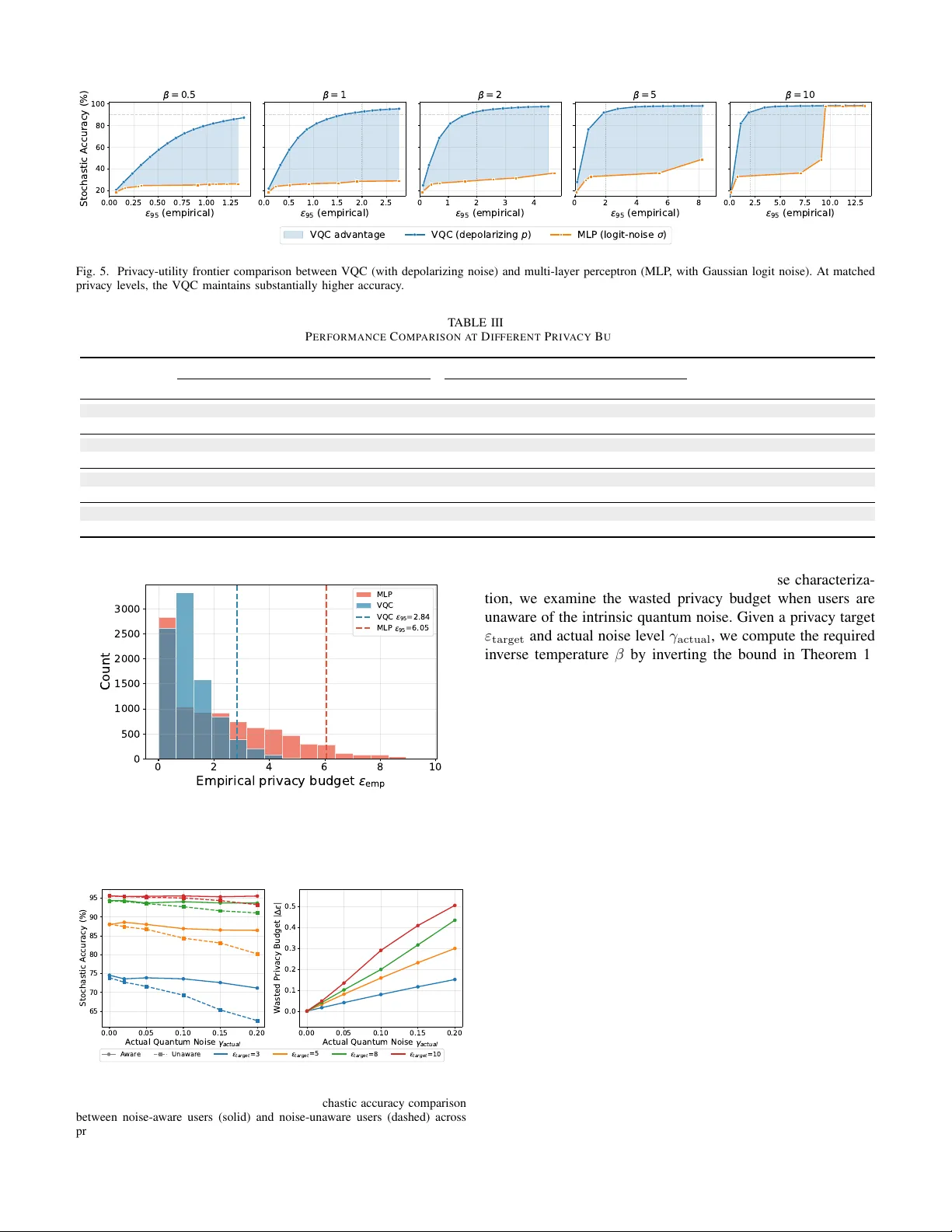
IEEE TRANSA CTIONS ON SMAR T GRID 1 Quantum-Enabled Probabilistic Optimal Po wer Flo w with Built-in Dif ferential Pri v ac y Y uji Cao, Graduate Student Member , IEEE , T ongxin Li, Y ue Chen, Senior Member , IEEE Abstract —Quantum computing has been regarded as a pr omis- ing approach to accelerate power system optimization. Ho wev er , challenges such as limited qubits and inherent noise hinder their widespread adoption in power systems. In this paper , we propose a qubit-efficient framew ork f or solving a crucial power system optimization problem, the pr obabilistic optimal power flow (POPF). W e demonstrate that quantum noise, traditionally viewed as a drawback, can in fact be leveraged to provide a built-in differ ential privacy (DP) guarantee. Specifically , we first linearize POPF into a multi-parametric linear program (MP- LP) with renewable uncertainties being the parameters. This decomposes the parameter space into critical regions with pre- computed solution maps. Second, a variational quantum cir cuit (VQC) classifies the critical region based on each uncertainty realization and then r ecovers the final solution. In this way , the requir ed qubits scale with the uncertain parameters instead of the network size, with only 5 qubits versus 600+ for direct quantum OPF in a 69-bus system. Moreover , we prov e the depolarizing noise of VQC provides DP guarantees and characterize the privacy-cost tradeoff. Case studies validate the proposed VQC achieves 2.1 × smaller privacy budgets compar ed to its classical counterpart. At matched privacy levels, the VQC also maintains lower infeasibility and pr ediction err or . Index T erms —Optimal power flow , quantum computing, dif- ferential privacy , multi-parametric linear programming I . I N T RO D U C T I O N T HE proliferation of rene wable energy sources is dri ving a global transition towards decarbonized power grids [1]. While these sources can lower carbon emissions, they also introduce significant volatility and uncertainty . T o address this challenge, probabilistic optimal power flow (POPF) is now a mainstream analytical framework. Its objectiv e is to assess the statistical characteristics of critical operating quantities under uncertainty . Howe ver , POPF requires e v aluating thousands to millions of scenarios and leads to a prohibiti ve computational burden for conv entional methods [2]. Quantum computing (QC) has emerged as a potential so- lution to such computationally intractable problems in power systems [3]. Unlike classical methods, QC exploits quantum- mechanical principles such as superposition and entanglement for computation. For problems with certain structures, QC is expected to provide exponential speedup over classical com- puters [4]. These prospects have motiv ated gro wing interest in applying QC to po wer systems optimization [5]. Ho we ver , Y . Cao and Y . Chen are with the Department of Mechanical and Automation Engineering, The Chinese Uni versity of Hong Kong, Hong Kong, China. (email: { yjcao, yuechen } @mae.cuhk.edu.hk) T . Li is with the School of Data Science, The Chinese Uni versity of Hong K ong, Shenzhen, China. (email: litongxin@cuhk.edu.cn). hardware challenges remain in current noisy intermediate-scale quantum (NISQ) de vices. A major hardware challenge is the limited number of quan- tum bits, i.e., qubits. T ypical OPF problems in volve hundreds of continuous decision v ariables. Solving these on quantum hardware requires discretizing each continuous variable into a binary representation, where the number of qubits per variable determines the precision. For hundreds of OPF variables, the required number of qubits f ar e xceeds current hardware capacity [6]. T o address this problem, one line of work [7] focuses on combinatorial OPF with discrete decision variables only and solves it via quantum annealing. Another work [8] decomposes the problem so that quantum hardware solves only the discrete subproblems, while continuous v ariables are handled by classical solvers. The quantum speedup is thus limited to the combinatorial component of the problem. The other major hardware challenge is the inevitable quan- tum noise [9], [10]. Indeed, imperfections in quantum hard- ware introduce errors that accumulate during computation and degrade the final results. T o suppress the noise, techniques such as quantum error mitigation and correction hav e been dev eloped [11], [12]. Despite these advances, full error correc- tion still requires substantial additional qubits and further lim- its the feasibility for near-term OPF applications. Meanwhile, near-term mitigation techniques offer only limited protection as circuit depth gro ws. As a result, non-ne gligible hardware noise remains unav oidable on near-term devices and must be accounted for when designing quantum optimization methods. Rather than vie wing the noise solely as a liability , recent work in information theory and statistics has shown that the intrinsic randomness of quantum noise can itself protect priv acy [13], [14]. This observation is particularly relev ant to the optimal power flow problem, which requires sensitiv e operational data such as customer loads and generator costs as input. OPF solutions, in turn, can be exploited to infer such priv ate data [15]. T o provide a rigorous priv acy guarantee, dif- ferential pri vacy (DP) mechanisms ha ve been widely applied to OPF problems, typically through artificial noise injection [16], [17]. By contrast, NISQ devices are inherently affected by hardware noise. This raises a natural question: does such built-in hardware noise already contribute to a meaningful DP guarantee for OPF , and if so, how strong is that contrib ution? W ithout answering this question, adding extra artificial noise on top of hardware noise is unnecessarily conservati ve and further degrades OPF solution quality . T o address the abov e challenges, this paper proposes a quantum-enabled framework for probabilistic OPF . W e reduce the qubit requirements by decomposing the parameter space 2 IEEE TRANSACTIONS ON SMAR T GRID into critical regions and using a v ariational quantum circuit (VQC) to identify the active region. Moreov er , instead of viewing inherent quantum noise as a liability , we use it as a natural random resource, prov e the DP guarantee and characterize the pri vac y-cost tradeof f. Our main contributions are two-fold: 1) A qubit-efficient quantum-enabled POPF framework: W e propose a quantum-enabled POPF framew ork built on multi-parametric linear programming (MP-LP) critical- region decomposition. The frame work precomputes affine solution maps for each critical region and uses a VQC to classify the active region during operation. This reduces the qubit requirement from encoding all decision and slack variables to classifying the activ e critical region. On a 69-bus system, the proposed frame work requires only 5 qubits, compared with 596 ∼ 1406 qubits required for direct encoding of OPF formulations at dif ferent precisions, with an estimated per-scenario speedup of ov er 9 , 000 × . 2) Privacy guarantees from inherent quantum noise: W e dev elop a depolarizing noise model for the proposed quantum-enabled POPF framework and prov e that it provides ( ε, 0) -differential priv acy . W e further bound the expected OPF cost increase under randomized dispatch and deri ve an explicit pri v acy-cost tradeoff. Case studies on a 69-bus system sho w that the VQC achie ves 2 . 1 × tighter priv acy bounds than a classical multi-layer per- ceptron (MLP). At matched pri vacy levels ( ε ≈ 3 ), the proposed quantum-enabled framework maintains 0.21% cost gap and 4.6% infeasibility , compared to 16.07% and 66.1% for the MLP with Gaussian noise. The remainder of this paper is organized as follows. Sec- tion II formulates POPF via multi-parametric programming. Section III presents the quantum classifier . Section IV analyzes priv acy guarantees and the priv acy-cost tradeof f. Case studies are conducted in Section V and conclusions are drawn in Section VI. I I . P RO B L E M F O R M U L A T I O N In this section, we first formulate the probabilistic optimal power flow (POPF) problem to be addressed. Then, we in- troduce a multi-parametric linear programming (MP-LP) ap- proach that partitions the parameter space into critical regions, within which the optimal solution can be expressed as an af fine function of the parameters. This reformulation transforms the POPF solving process into identifying the critical region corresponding to the given parameters, which significantly reduces the number of qubits required for computation. A. Pr obabilistic OPF and Linearization The POPF problem seeks to calculate the expected min- imum operational cost of po wer systems ov er uncertainty , such as renew able generation and load demand. For each uncertainty scenario, denoted by θ , a deterministic OPF is solved. The POPF problem is formulated as: E θ h min u f ( u, θ ) i , (1a) s.t. h ( u, θ ) = 0 , (1b) g ( u, θ ) ≤ 0 , (1c) where u denotes the decision variables (e.g., thermal generator setpoints, voltage magnitudes), θ is a vector of uncertain parameters, and f ( · ) is the operational cost. h ( · ) = 0 and g ( · ) ≤ 0 encode the equality and inequality operational constraints, respectively . Evaluating the expectation in (1) typically requires Monte Carlo sampling, where the inner optimization problem is solved repeatedly for a lar ge number of uncertainty scenarios. The inner optimization for each scenario is an OPF problem. Consider a network with a bus set N , a generator set G , and a line set L . Let G i ⊆ G denote generators at bus i . The standard alternating current (A C) OPF problem that minimizes the total generation cost subject to power balance and operational limits is gi ven by min P g ,Q g ,V ,δ X g ∈G C g ( P g ) , (2a) s.t. V i X j ∈N V j  G ij cos δ ij + B ij sin δ ij  = X g ∈G i P g − P d,i , ∀ i ∈ N , (2b) V i X j ∈N V j  G ij sin δ ij − B ij cos δ ij  = X g ∈G i Q g − Q d,i , ∀ i ∈ N , (2c) P g ≤ P g ≤ P g , Q g ≤ Q g ≤ Q g , ∀ g ∈ G , (2d) V i ≤ V i ≤ V i , ∀ i ∈ N , (2e) where P g and Q g are the active and reactiv e power outputs of generator g , P d,i and Q d,i are the active and reactiv e demands at bus i , and V i and δ i are the voltage magnitude and angle with δ ij := δ i − δ j . The terms G ij and B ij are elements of the bus admittance matrix Y = G + j B , and C g ( · ) is the generation cost function. Constraints (2b)–(2c) enforce po wer balance at each bus, while (2d)–(2e) impose operational limits. The power flow equations (2b) and (2c) make the AC- OPF problem noncon ve x. V arious linearization methods hav e been developed to obtain tractable approximations, including direct current (DC) power flo w models [18], LinDistFlo w for radial networks [19], and second-order cone programming relaxation [20] plus polyhedral approximations [21]. When such linearization is applied, the A C-OPF model (2) reduces to a linear programming (LP) problem. Although the linearized OPF is an LP , ev aluating the expectation in (1) still requires one LP per uncertainty sce- nario. For large-scale Monte Carlo simulations with thousands of scenarios, this repeated computation remains expensi ve. Quantum computing has the great potential to accelerate such workloads, but current NISQ devices provide only tens to hundreds of qubits. The full OPF decision vector may contain hundreds of v ariables, far exceeding this capacity . T o facilitate the implementation with limited qubits, in the following, we propose a multi-parametric programming-based reformulation CA O ET AL.: QUANTUM-EN ABLED PROB ABILISTIC OPTIMAL POWER FLOW WITH BUIL T -IN DIFFERENTIAL PRIV ACY 3 method, which reduces the OPF problem to a classification problem ov er a low-dimensional parameter space. B. Multi-parametric Linear Pr ogramming Reformulation When the inner OPF problem is linearized, treating the uncertainties as parameters yields a multi-parametric linear programming (MP-LP). Let x ∈ R n denote the decision variables and θ ∈ R m the uncertain parameters. The problem can be e xpressed in a compact parametric form: x ∗ ( θ ) = arg min x c ⊤ x, s.t. W x ≤ S + T θ, (3) where c ∈ R n is the cost coefficient vector , W ∈ R q × n and S ∈ R q encode the constraint coef ficients, and T ∈ R q × m determines how the uncertain parameters θ enter the constraint right-hand side. The parameter θ ranges over a bounded poly- tope Θ ⊂ R m determined by feasible load and/or generation bounds. Equality constraints (e.g., power balance) are handled by elimination or by e xpressing them as paired inequalities. This MP-LP reformulation recasts the computational task. A key result from MP-LP theory is that the parameter space Θ can be partitioned into a finite number (say K ) of con ve x polyhedral sets, known as critical regions (CRs). W ithin each critical region k , denoted by CR k , the set of active constraints at the optimal solution remains in variant. This in variance implies that the optimal solution vector x ∗ ( θ ) becomes a direct affine function of the parameter θ : x ∗ ( θ ) = F k θ + f k , ∀ θ ∈ CR k . (4) T o obtain F k and f k , consider the set of active constraints within CR k . Let A k denote the index set of constraints that are binding at the optimal solution. These constraints satisfy W A k x ∗ ( θ ) = S A k + T A k θ , (5) where W A k , S A k , and T A k are the rows of W , S , and T index ed by A k . Assuming the activ e constraint matrix has full column rank and, in the non-degenerate case, consists of n linearly independent constraints, W A k ∈ R n × n is nonsingular . Therefore, x ∗ ( θ ) = W − 1 A k S A k + W − 1 A k T A k θ . (6) Applying (4) to (6), it follows that F k = W − 1 A k T A k , f k = W − 1 A k S A k . The in verse formula abov e applies in the non-degenerate case, where the activ e matrix contains n linearly independent binding constraints. In a degenerate region, more than n constraints may be binding, and multiple primal or dual optimal solutions may mak e the construction of critical regions from optimal basis inv ariance difficult. Follo wing [22], in this paper we first recover the critical region from a dual or value- function representation and then recover the corresponding primal solution. Therefore, the piecewise-af fine representation in (4) is preserv ed. The critical region decomposition transforms the solution of the OPF problem into a more manageable two-stage process. First, a multi-class classification is performed: for a giv en uncertainty scenario θ , one must identify the critical region CR k it belongs to. Since each critical region corresponds to a unique activ e constraint set A k , the binding constraints are directly determined once the region index k is known. Second, once the re gion is identified, the full, high-dimensional optimal solution x ∗ ( θ ) is recovered with negligible computation via the simple affine solution map in (4). This transformation shifts the computational burden from high-dimensional regression to classification. Rather than regressing all n OPF decision variables, the problem reduces to identifying the region index k , from which the full solution is recovered analytically via (4). This classification is well-suited to quantum computing because quantum feature maps embed the high-dimensional uncertainty parameter θ into an exponentially large Hilbert space [23], providing richer representational po wer for sep- arating critical regions than classical methods of comparable complexity . I I I . H Y B R I D Q UA N T U M - C L A S S I C A L C L A S S I FI E R F O R P RO B A B I L I S T I C O P F This section presents the hybrid quantum-classical classi- fier for fast critical region identification. In the classifier, a variational quantum circuit architecture extracts features from the encoded uncertainty parameters. A classical netw ork then maps these features to region scores, and a temperature- controlled softmax produces region probabilities, enabling tunable tradeoffs between classification confidence and output randomness. A. V ariational Quantum F eatur e Extr actor T o identify the critical region that contains a giv en uncer- tainty scenario θ , we employ a v ariational quantum classifier . Its fundamental component is the variational quantum circuit (VQC), which uses a parameterized quantum circuit as a trainable feature map to learn complex representations in the high-dimensional Hilbert space of the quantum system [24]. The VQC maps the uncertainty θ to a set of distinguishing features to separate the K critical regions. Layer L Layer 1 Data reuploading Fig. 1. V ariational quantum feature extractor with data reuploading technique. Each layer re-encodes input θ via R y gates, followed by trainable U ϕ gates and CNOT entanglement. Measurements on all qubits yield the feature vector h . As illustrated in Fig. 1, the VQC transforms the classical input θ ∈ R m into the feature vector h through a layered quantum circuit followed by measurement. The circuit acts on n q qubits initialized in the ground state | 0 ⟩ ⊗ n q , producing 4 IEEE TRANSACTIONS ON SMAR T GRID an output state | ψ out ⟩ from which classical information is extracted. The ket notation |·⟩ denotes a quantum state vector in a 2 n q -dimensional space. Each feature h i is the Pauli- Z expectation value on qubit i , a real number in [ − 1 , 1] indicating whether qubit i is more likely measured in state | 0 ⟩ (yielding +1 ) or | 1 ⟩ (yielding − 1 ): h i = ⟨ ψ out | σ ( i ) z | ψ out ⟩ , i = 1 , . . . , n q . (7) A con ventional VQC architecture encodes the classical input data only once initially , then applies trainable gates. Howe ver , such single-encoding circuits have limited expressi vity: their outputs are restricted to Fourier series with frequencies de- termined solely by the encoding gates [25]. This limits the circuit’ s ability to learn complex, nonlinear decision bound- aries required for accurate re gion classification. T o address this limitation, we adopt the data r euploading technique [26], which interleav es data encoding with trainable gates across multiple layers. By re-encoding θ at each layer , the circuit can represent richer function classes with higher- frequency Fourier components [25]. This design is particularly suitable for near -term quantum devices, as it achie ves greater expressi vity without requiring additional qubits. Specifically , the circuit in Fig. 1 comprises L repeated layers. Each layer ℓ consists of three operations applied sequentially: 1) Data encoding: The input θ is encoded via single-qubit R y rotations. For qubit i , the gate is defined as: R y ( θ i ) = exp  − i θ i 2 σ y  =  cos θ i 2 − sin θ i 2 sin θ i 2 cos θ i 2  , (8) where θ i is determined by a corresponding component of θ (with appropriate preprocessing when m  = n q ). 2) T rainable rotations: Parameterized single-qubit gates R y ( ϕ ( ℓ ) i ) are applied, where ϕ ( ℓ ) i are learnable parameters optimized during training. This enables the circuit to learn task-specific transformations. 3) Entanglement: CNOT gates arranged in a ladder topol- ogy create correlations between neighboring qubits: U ent = n q − 1 Y i =1 CNO T i,i +1 , (9) where CNOT i,j flips qubit j conditioned on qubit i . This entanglement allows the circuit to capture multi-feature interactions that cannot be represented by product states. The full circuit is gi ven by the composition of all layers: U ( ϕ q , θ ) = L Y ℓ =1 h U ent · U ( ℓ ) ϕ · U E ( θ ) i , (10) where U E ( θ ) = N n q i =1 R y ( θ i ) denotes the data-encoding layer , and U ( ℓ ) ϕ = N n q i =1 R y ( ϕ ( ℓ ) i ) the trainable layer . The output state is: | ψ out ⟩ = U ( ϕ q , θ ) | 0 ⟩ ⊗ n q . (11) Finally , classical information can be extracted from the final quantum state | ψ out ⟩ , by measuring the Pauli-Z expectation value on each qubit. For qubit i , the feature is: h i = ⟨ ψ out | σ ( i ) z | ψ out ⟩ = p (0) i − p (1) i , (12) where p (0) i and p (1) i are the probabilities of measuring qubit i in state | 0 ⟩ and | 1 ⟩ , respectiv ely . In practice, these expectation values are estimated by repeated circuit executions (shots) and av eraging the measurement outcomes. This quantum-extracted vector h encodes a rich feature representation of the input θ , which includes high-order cor- relations learned by the VQC and thus provides a po werful basis for the subsequent netw ork. B. T emperatur e-Controlled Region Classifier Building on representations learned from the VQC, a clas- sical network maps the compact representation to region scores and learns weights that determine how features are combined to distinguish each region. A softmax function with in verse temperature β then con verts these scores to selection probabilities. Once a region is selected, the full OPF solution is reconstructed via the precomputed affine solution map (4). The VQC feature vector h is passed to a linear classifier that produces logits s = W cl h + b cl , where W cl and b cl are weights and biases. A softmax with in verse temperature β > 0 con verts these logits to re gion selection probabilities: p k = exp( β s k ) P K j =1 exp( β s j ) . (13) The parameter β controls the sharpness of the output dis- tribution: lar ge β concentrates probability mass on the top- scoring re gion for accurate classification, while small β flattens the distribution toward uniform. During training, quantum parameters ϕ q and classical parameters ϕ c = { W cl , b cl } are trained jointly by minimizing cross-entropy loss, with quantum gradients obtained via the parameter -shift rule [27] below: ∂ L ∂ ϕ = 1 2 [ L ( ϕ + π / 2) − L ( ϕ − π / 2)] . (14) These gradients are then fed to a classical optimizer such as Adam to update all model parameters. The complete offline training and online inference proce- dures are detailed in Algorithm 1. Once trained, the model of- fers a substantial acceleration for POPF analysis. For any new uncertainty scenario θ new , the hybrid classifier rapidly infers the corresponding critical re gion index k . Subsequently , the full, high-dimensional OPF solution vector x ∗ ( θ new ) is recon- structed with negligible computation on a classical computer via the affine transformation in (4). This paradigm addresses the dimensionality challenge of near-term quantum devices by shifting the computational task from high-dimensional regression to low-dimensional classification. Howe ver , deploying this quantum classifier on near-term hardware raises two practical concerns. First, noise in cur- rent quantum hardware distorts the measured features h and degrades classification accuracy . Second, the released region index ˜ k may leak sensitiv e information about the operating condition θ , such as individual load patterns or rene wable generation. A ke y observation is that these two concerns are inherently coupled. The same quantum noise that degrades classification accuracy also obscures the mapping from θ to ˜ k , which is a natural mechanism for priv acy protection. In the CA O ET AL.: QUANTUM-EN ABLED PROB ABILISTIC OPTIMAL POWER FLOW WITH BUIL T -IN DIFFERENTIAL PRIV ACY 5 Algorithm 1 A Hybrid Quantum-Classical POPF Algorithm 1: Offline Phase: T raining Require: T raining data { ( θ i , k i ) } N i =1 , affine solution maps { ( F k , f k ) } K k =1 , Epochs E , batch size B , learning rate η 2: Initialize ϕ q and ϕ c = { W cl , b cl } 3: for epoch = 1 to E do 4: for each mini-batch B do 5: Forward: U ( ϕ q , θ ) | 0 ⟩ ⊗ n q → h → softmax ( W cl h + b cl ) 6: Compute cross-entropy loss L 7: Gradients: backprop ( ϕ c ) + parameter -shift ( ϕ q ) 8: Update: ϕ q ← ϕ q − η ∇ ϕ q L , ϕ c ← ϕ c − η ∇ ϕ c L 9: end f or 10: end for 11: Store trained parameters ( ϕ ∗ q , ϕ ∗ c ) 1: Online Phase: Privacy-Preserving Inference Require: Ne w scenario θ new , temperature β , noise le vel γ 2: Process with noise: ρ out = E γ  U ( ϕ ∗ q , θ new ) | 0 ⟩ ⟨ 0 | ⊗ n q U † ( ϕ ∗ q , θ new )  3: Measure: h j = T r( σ ( j ) z ρ out ) for j = 1 , . . . , n q 4: Compute logits: s = W ∗ cl h + b ∗ cl 5: Compute probabilities: p k = exp( β s k ) / P K j =1 exp( β s j ) 6: Sample region: ˜ k ∼ Categorical ( p ) 7: Reconstruct solution: x ∗ = F ˜ k θ new + f ˜ k Ensure: Region index ˜ k (released), OPF solution x ∗ next section, we formalize this observation and quantify the resulting pri v acy-accurac y tradeof f. I V . P R I V A C Y A NA LY S I S Hardware noise is an inherent feature of near-term quantum devices. This section sho ws that such noise provides differen- tial priv acy for the released region index. W e first define the inherent quantum noise and formalize how depolarizing noise affects the output distribution, then prove the main priv acy guarantee, and finally characterize the priv acy-cost tradeof f. A. Inherent Quantum Noise W e assume an adversary observes the region index ˜ k released by the online dispatch pipeline and attempts to infer sensitiv e information about the current operating point θ (e.g., customer loads or renew able generation). Our objecti ve is to ensure that the distribution of ˜ k is insensitive to small perturbations of θ , formalized by the following adjacency relation. Definition 1 (Parameter Adjacency) . F or a fixed ∆ θ > 0 , two parameter vectors θ , θ ′ ∈ R m ar e adjacent (denoted by θ ∼ θ ′ ) if ∥ θ − θ ′ ∥ 2 ≤ ∆ θ . The radius ∆ θ bounds the perturbation for which outputs should remain indistinguishable. In power systems, this cor- responds to operationally similar scenarios, such as a 5% fluctuation in rene wable generation or load demand. Our goal is to provide priv acy guarantees to ensure that an adversary cannot distinguish such neighboring conditions by observing the released re gion index. In this paper , we argue that the inherent quantum noise can obscure the released region index and thus protect priv acy . First, we model quantum hardware errors using the depo- larizing channel, a standard noise model that approximates the aggregate effect of gate errors in near-term quantum processors [28]. F or any quantum state ρ on n q qubits, the depolarizing channel with noise le vel γ ∈ (0 , 1) is defined as follows: E γ ( ρ ) = (1 − γ ) ρ + γ I D . (15) That is, with probability 1 − γ , the state is preserved; with prob- ability γ , it is replaced by I /D , with D = 2 n q and I ∈ R D × D is the identity matrix. The state I /D represents complete loss of information, in which all measurement outcomes are equally likely . Let ρ ( θ ) denote the density matrix of the quantum state after encoding the input θ via the data-reuploading circuit. Under this noise model, the measured feature on qubit j becomes h j ( θ ) = T r  σ ( j ) z E γ  U ( ϕ q ) ρ ( θ ) U † ( ϕ q )   . (16) The noise level γ controls the contraction strength. Larger γ flattens the output distrib ution to ward uniform, which strength- ens pri v acy b ut reduces classification accuracy . W e make the follo wing assumption: Assumption 1 (Lipschitz Encoding) . Ther e exists L enc ≥ 0 such that for all θ , θ ′ , D tr ( ρ ( θ ) , ρ ( θ ′ )) ≤ L enc ∥ θ − θ ′ ∥ 2 , (17) wher e D tr ( ρ, ρ ′ ) := 1 2 ∥ ρ − ρ ′ ∥ 1 is the tr ace distance. The trace distance D tr ( ρ, ρ ′ ) quantifies how distinguishable two quantum states are, ranging from zero (identical) to one (orthogonal). Assumption 1 requires that nearby parameters produce similar quantum states, with L enc bounding the en- coding’ s sensitivity . This assumption is satisfied by common encoding schemes such as angle encoding [29], [30], where the rotation angles depend continuously on the input. It links parameter-space adjacency to quantum-state proximity . B. Differ ential Privacy Guarantee In the following, we analyze how the inherent quantum noise can protect priv acy . W e first present the concept of differential priv acy . Definition 2 (Dif ferential Priv acy [31]) . A r andomized mec h- anism M : Θ → Y satisfies ( ε, 0) -differ ential privacy if for any adjacent θ ∼ θ ′ and any measur able set S ⊆ Y , P [ M ( θ ) ∈ S ] ≤ e ε P [ M ( θ ′ ) ∈ S ] . (18) Based on this definition, the follo wing theorem quantifies the priv acy budget ε of Algorithm 1 in terms of the depolar- izing noise le vel γ and inv erse temperature β . Theorem 1 (Re gion-ID Differential Priv acy) . Under Assump- tion 1, the randomized mechanism in Algorithm 1 that maps θ to the released r egion inde x ˜ k satisfies ( ε reg , 0) -differ ential privacy over the output space Y = { 1 , . . . , K } , wher e ε reg ≤ 4 β (1 − γ ) L enc ∆ θ ∥ W cl ∥ ∞ , 1 , (19) 6 IEEE TRANSACTIONS ON SMAR T GRID with ∥ W cl ∥ ∞ , 1 := max k ∥ w k ∥ 1 denoting the maximum ℓ 1 - norm of the r ows of the weight matrix W cl in the linear classifier . The proof of Theorem 1 can be found in Appendix A. It shows that depolarizing noise uniformly contracts quantum expectation values, reducing the sensitivity of output proba- bilities to input perturbations. C. Privacy-Cost T radeoff The priv acy guarantee in Theorem 1 comes at a cost: randomized region selection may result in an incorrect region, leading to a suboptimal dispatch. This section quantifies the expected cost increase and establishes an explicit tradeoff between pri v acy and operational efficiency . Let J ( x ; θ ) denote the operational cost when solution x is applied under parameter θ . For any re gion k , the affine solution from (4) is x k ( θ ) = F k θ + f k , and the classifier logit from (13) is s k ( θ ) . Let k ∗ ( θ ) denote the correct region containing θ , with optimal solution x ∗ ( θ ) = F k ∗ θ + f k ∗ . Define the cost gap for selecting region k as ∆ J k ( θ ) := J ( x k ( θ ); θ ) − J ( x ∗ ( θ ); θ ) . Under randomized dispatch, the realized cost gap is ∆ J := ∆ J ˜ k ( θ ) , where ˜ k is the sam- pled region index. The score margin m ( θ ) := s k ∗ ( θ ) − max k  = k ∗ s k ( θ ) measures the logit margin between the correct region and the highest-scoring competing region. A larger positiv e margin indicates clearer separation. Theorem 2 (Priv acy-Cost T radeoff) . Let ∆ J max ( θ ) := max k  = k ∗ ∆ J k ( θ ) . Under softmax sampling with inverse tem- peratur e β , E [∆ J | θ ] ≤ ∆ J max ( θ ) | {z } worst-case cost gap · ( K − 1) exp( − β m ( θ )) | {z } mis-selection pr obability bound , (20) wher e ∆ J max ( θ ) captures the maximum cost penalty fr om selecting a wr ong r egion, while ( K − 1) exp( − β m ( θ )) bounds the pr obability of such mis-selection via the softmax margin m ( θ ) . The proof of Theorem 2 is provided in the Appendix B. It proceeds in three parts: first establishing the cost decom- position, then bounding the mis-selection probability via the softmax margin, and finally combining them to deriv e the tradeoff. Remark 1 (Simplified Bound for Standard VQC) . F or stan- dar d variational quantum cir cuits using P auli- Z measurements and no classifier bias ( b cl = 0 ), the mar gin scales linearly with noise: m ( θ ) = (1 − γ ) m (0) ( θ ) , wher e m (0) ( θ ) is the noiseless mar gin. This yields a simplified bound: E [∆ J | θ ] ≤ ∆ J max ( θ ) · ( K − 1) exp  − β (1 − γ ) m (0) ( θ )  . Remark 2 (T uning the Priv acy-Cost Tradeof f) . The privacy budg et ε reg and expected cost incr ease are both contr olled by β (1 − γ ) . Increasing γ (mor e noise) or decreasing β (softer sampling) impr oves privacy but raises cost. Eliminating β (1 − γ ) between Theor ems 1 and 2 yields an explicit r elationship: for standar d VQC (Remark 1), E [∆ J | θ ] ≤ ∆ J max ( θ ) · ( K − 1) exp  − m (0) ( θ ) 4 L enc ∆ θ ∥ W cl ∥ ∞ , 1 ε reg  . Given a privacy budget ε reg , the cost bound decays expo- nentially with ε reg , and the decay rate impr oves with larg er mar gin m (0) . 1 2 3 4 5 6 7 8 9 10 11 12 13 14 15 16 17 18 19 20 40 41 55 56 57 58 59 60 61 62 63 64 65 66 67 68 69 21 22 23 24 25 26 27 31 30 29 28 32 33 34 35 36 37 38 39 42 43 44 45 46 47 48 49 50 51 52 53 54 Fig. 2. T opology of 69-bus distribution network. -10 10 -5 5 0 10 Wind 3 5 5 Wind 2 0 Wind 1 10 0 -5 -5 -10 -10 Fig. 3. The critical regions of the multi-parametric LP problem for the 69-bus distribution network. V . C A S E S T U DY W e test our method on a modified 69-bus distribution network [32]. The topology is shown in Fig. 2. Six elastic demands are located at nodes 12, 23, 32, 42, 53 and 62, re- spectiv ely . Three renewable generators are connected to nodes 9, 30, and 60, respectiv ely . Their real-time de viations fall within [ − 10 , 10] kW . Using these de viations as the uncertainty parameter θ = [∆ w 1 , ∆ w 2 , ∆ w 3 ] ⊤ and applying the MP- LP method described in (3), we obtain sev en critical regions as shown in Fig. 3. 3,000 data points are sampled from the uncertainty space and used to train the variational quantum classifier with uncertainty parameters normalized to [ − 1 , 1] . T ABLE I M O DE L A R CH I T E CT U R E A N D P E R FO R M AN C E C O M P A R IS O N VQC MLP Architecture 5 qubits, 6 layers 3 → 7 → 7 → 7 Parameters 125 133 T est Accuracy (%) 98.23 97.78 CA O ET AL.: QUANTUM-EN ABLED PROB ABILISTIC OPTIMAL POWER FLOW WITH BUIL T -IN DIFFERENTIAL PRIV ACY 7 A VQC and a multi-layer perceptron (MLP) are trained to predict the region index based on the uncertainty param- eters. T able I summarizes the model architectures and their performance. The VQC uses 5 qubits with 6 variational layers, each consisting of angle encoding gates followed by strongly entangling CNO T gates. The MLP uses 2 hidden layers with 7 neurons each, matching the VQC’ s parameter count. A linear layer without bias is appended to both models. Both models are trained for 30 epochs using Adam optimizer (learning rate 0.05, batch size 32) with cross-entropy loss under noise-free conditions. The VQC is implemented in PennyLane [33] and the MLP in PyT orch [34]. A. Privacy Guarantees and T rade-offs 0.0 0.1 0.2 0.3 0.4 0.5 D e p o l a r i z i n g n o i s e 0 2 4 6 8 10 12 9 5 ( e m p i r i c a l ) (a) P rivacy vs Noise Inverse temp. =0.1 =0.2 =0.3 =0.5 =0.7 =1.0 =1.5 =2.0 =3.0 =5.0 =7.0 =10.0 0 2 4 6 8 10 12 9 5 ( e m p i r i c a l ) 20 30 40 50 60 70 80 90 100 Stochastic A ccuracy (%) (b) P rivacy -Utility T radeoff Inverse temp. =0.1 =0.2 =0.3 =0.5 =0.7 =1.0 =1.5 =2.0 =3.0 =5.0 =7.0 =10.0 Fig. 4. Privac y-utility frontier showing stochastic accuracy versus empirical ε for different in verse temperatures β . Each curve traces the effect of varying noise γ from 0 to 0.5. The randomized region-selection mechanism provides tun- able priv acy through two parameters: the depolarizing noise lev el γ and the in verse temperature β . This subsection vali- dates the differential priv acy guarantee established in Theo- rem 1, characterizes the resulting pri vacy-utility tradeoff, and compares the VQC against a classical MLP baseline. T o empirically assess the priv acy b udget, we construct 100 adjacent input pairs and measure how the output distribution changes. The adjacent parameters θ and θ ′ are bounded by ∆ θ = 0 . 05 with ∥ θ − θ ′ ∥ 2 ≤ ∆ θ in the normalized feature space, corresponding to approximately 1 kW perturbation in load or renewable generation. For each pair, we compute the empirical pri v acy b udget ε emp ( θ , θ ′ ) = max k     log P k ( θ ) P k ( θ ′ )     , (21) which measures the maximum log-ratio of output probabilities. W e report ε 95 , the 95th percentile over adjacent pairs, as an empirical pri vacy indicator that is robust to outliers. Note that ε 95 is a statistical summary of observed log-ratios, not a formal DP guarantee; the formal worst-case bound is ε reg from Theorem 1. The left figure in Fig. 4 analyzes the effects of noise and temperature. W e e v aluate ε 95 for γ ∈ { 0 , 0 . 1 , 0 . 2 , 0 . 3 , 0 . 4 , 0 . 5 } and β from 0.1 to 10. As predicted by Theorem 1, increasing depolarizing noise γ reduces the priv acy budget ε 95 due to the (1 − γ ) factor . Similarly , decreasing the inv erse temperature β flattens the softmax distribution, further reducing ε 95 . The right figure reveals the resulting priv acy-utility tradeoff by ev aluating the accuracies for all ( γ , β ) combinations. The result collapses into a single frontier . The frontier exhibits a steep transition region: accuracy de grades rapidly below ε 95 ≈ 3 , where priv acy constraints begin to dominate, but remains abov e 90% for ε 95 ≥ 3 . This characterization allows operators to analyze the tradeoff between priv acy and accuracy and select an optimal parameter configuration based on their priv acy requirements. Fig. 5 compares the priv acy-utility frontiers of the VQC and a classical MLP baseline across different inv erse temperatures. The MLP baseline shares the same classical head architecture as the VQC. T o introduce priv acy , independent Gaussian noise N (0 , σ 2 ) is added to the MLP logits before softmax sampling. For each target pri vacy le vel, the noise scale σ is tuned until the resulting ε 95 matches the target, using the same ev aluation protocol (100 adjacent pairs, ∆ θ = 0 . 05 ) as for the VQC. In the figures, we can observe a gap (shaded area) between the accuracy of VQC and MLP , indicating that the VQC achiev es higher accuracy than the MLP at matched ε 95 . The advantage is more notable at low β : at β = 1 and ε 95 ≈ 1 , the VQC achieves approximately 80% accuracy while the MLP remains near 27%, which is barely abov e random guessing for seven critical regions. Even at higher β values where the MLP ev entually reaches high accuracy , it requires significantly larger ε 95 . This consistent gap demonstrates that depolarizing noise provides a more fav orable priv acy-utility tradeoff than additiv e Gaussian noise on classical logits. T o explain this advantage, we examine the baseline case without depolarizing noise. At γ = 0 and β = 1 , the VQC achiev es ε 95 = 2 . 84 while the MLP yields ε 95 = 6 . 05 , a 2 . 1 × difference even without any priv acy-enhancing mechanism. Fig. 6 visualizes the distribution of empirical priv acy budget ov er adjacent pairs: the VQC distribution concentrates at lo wer values with 95% belo w 2.84, while the MLP tail extends beyond 6. T ABLE II P RO BA B I LI T Y D I S T RI B U TI O N S E N S IT I V IT Y T O I N P UT P E RT UR B A T I ON Probability P k ′ Method P k ∗ ( θ ) P k ′ ( θ ) P k ′ ( θ ′ ) Ratio ε emp MLP 0 . 998 3 . 9 × 10 − 7 2 . 4 × 10 − 5 61 × 4.11 VQC 0 . 960 7 . 6 × 10 − 3 2 . 3 × 10 − 2 3 . 0 × 1.11 P k ∗ : top-1 probability; P k ′ : class maximizing | log( P k /P ′ k ) | . Same input pair , ∥ θ − θ ′ ∥ 2 = 0 . 05 . W e e xamine specific adjacent input pairs to in vestigate this gap further and compare the prediction probabilities of both models. As sho wn in T able II, the MLP e xhibits severe over - confidence: its top-1 probability P k ∗ reaches 0 . 998 , forcing other class probabilities to near-zero (e.g., P k ′ < 10 − 6 ). When the input is slightly perturbed, these near-zero probabilities shift by orders of magnitude, causing the probability ratio to elev ate ( 61 × ) and yielding high ε emp . In contrast, the VQC maintains relativ ely moderate confidence ( P k ∗ = 0 . 960 ), with smoother probability distributions and less sensitivity to perturbations. This difference arises from the VQC’ s architec- tural constraint: its outputs are expectation values of Pauli- Z measurements, inherently bounded in [ − 1 , +1] , which acts as implicit regularization against overconfidence. 8 IEEE TRANSACTIONS ON SMAR T GRID 0.00 0.25 0.50 0.75 1.00 1.25 9 5 ( e m p i r i c a l ) 20 40 60 80 100 Stochastic A ccuracy (%) = 0 . 5 0.0 0.5 1.0 1.5 2.0 2.5 9 5 ( e m p i r i c a l ) = 1 0 1 2 3 4 9 5 ( e m p i r i c a l ) = 2 0 2 4 6 8 9 5 ( e m p i r i c a l ) = 5 0.0 2.5 5.0 7.5 10.0 12.5 9 5 ( e m p i r i c a l ) = 1 0 VQC advantage V Q C ( d e p o l a r i z i n g p ) M L P ( l o g i t - n o i s e ) Fig. 5. Priv acy-utility frontier comparison between VQC (with depolarizing noise) and multi-layer perceptron (MLP , with Gaussian logit noise). At matched priv acy levels, the VQC maintains substantially higher accuracy . T ABLE III P E RF O R M AN C E C O M P A RI S O N AT D I FFE R E N T P R IV AC Y B U D GE T S Generator Prediction Error (MW) Power Flow Prediction Error (MW) Method ε P g, 1 P g, 2 P g, 3 P g, 4 P g, 5 P g, 6 P l, 10 P l, 9 P l, 8 P l, 7 P l, 6 P l, 4 MAE Cost Gap Infeas. (%) VQC 0.9 0.533 0.751 0.201 0.083 0.280 0.594 0.721 0.721 0.721 0.552 0.552 0.552 0.522 4.96% 23.6% MLP 1.0 2.528 2.758 0.459 0.436 1.657 2.530 3.517 3.517 3.517 2.753 2.753 2.753 2.432 16.72% 67.3% VQC 2.8 0.030 0.038 < 0.01 < 0.01 0.019 0.041 0.054 0.054 0.054 0.042 0.042 0.042 0.036 0.21% 4.6% MLP 3.3 2.386 2.608 0.433 0.402 1.586 2.398 3.361 3.361 3.361 2.617 2.617 2.617 2.312 16.07% 66.1% VQC 5.0 0.014 0.018 < 0.01 < 0.01 < 0.01 0.023 0.030 0.030 0.030 0.023 0.023 0.023 0.019 0.09% 2.2% MLP 5.4 1.975 2.313 0.497 0.301 1.159 1.962 2.800 2.800 2.800 2.210 2.210 2.210 1.936 13.47% 63.9% VQC 9.7 0.012 0.017 < 0.01 < 0.01 < 0.01 0.021 0.027 0.027 0.027 0.021 0.021 0.021 0.017 0.08% 1.8% MLP 10.3 0.883 1.036 0.163 0.227 0.602 1.003 1.519 1.519 1.519 1.112 1.112 1.112 0.984 5.52% 45.1% 0 2 4 6 8 10 E m p i r i c a l p r i v a c y b u d g e t e m p 0 500 1000 1500 2000 2500 3000 Count MLP VQC V Q C 9 5 = 2 . 8 4 M L P 9 5 = 6 . 0 5 Fig. 6. Distribution of empirical pri vac y budget ε emp over adjacent pairs. The VQC (blue) has a shorter tail than the MLP (red), yielding ε 95 = 2 . 84 vs. 6 . 05 . 0.00 0.05 0.10 0.15 0.20 A c t u a l Q u a n t u m N o i s e a c t u a l 65 70 75 80 85 90 95 Stochastic A ccuracy (%) 0.00 0.05 0.10 0.15 0.20 A c t u a l Q u a n t u m N o i s e a c t u a l 0.0 0.1 0.2 0.3 0.4 0.5 W a s t e d P r i v a c y B u d g e t | | A war e Unawar e t a r g e t = 3 t a r g e t = 5 t a r g e t = 8 t a r g e t = 1 0 Fig. 7. Noise-awareness benefit for priv acy-utility tradeoff. Left: wasted pri- vac y budget | ∆ ε | due to unawareness. Right: stochastic accuracy comparison between noise-aw are users (solid) and noise-unaware users (dashed) across priv acy targets ε ∈ { 3 , 5 , 8 , 10 } . Noise-aware users achiev e up to 8.65% higher accuracy at the same privac y lev el. T o further explore the practical value of noise characteriza- tion, we examine the wasted priv acy budget when users are unaware of the intrinsic quantum noise. Giv en a priv acy target ε target and actual noise lev el γ actual , we compute the required in verse temperature β by inv erting the bound in Theorem 1: aware users substitute the true γ actual , while unaw are users conservati vely assume γ = 0 . Since intrinsic noise already contributes to pri vacy protection via the (1 − γ ) factor , a ware users need less additional uncertainty from softmax sampling and can use a lar ger β . Fig. 7 quantifies the resulting inefficienc y . The left figure shows the wasted priv acy budget: unaware users unknowingly achiev e ε actual = ε target (1 − γ ) < ε target , providing stronger protection than required. The wasted priv acy budget grows nearly linearly with γ actual , reaching | ∆ ε | = 0 . 5 at ε target = 10 and γ = 0 . 2 . The right figure shows the corresponding accuracy loss: aware users (solid) consistently outperform unaware users (dashed), with the gap reaching nearly 10% at ε target = 3 and γ = 0 . 2 . B. Analysis of Operational F easibility Practical deployment requires that the randomized region selection does not sev erely compromise operational feasibility or economic performance. In this section, we e v aluate three metrics: prediction error for key decision variables (generators and line flows), constraint feasibility under the affine dispatch policy , and the economic performance in terms of cost gap. W e compute the affine solution map x = F ˜ k θ + f ˜ k for the predicted region ˜ k and check whether all constraints W x ≤ S + T θ are satisfied. The maximum violation threshold is 10 − 4 . For cost ev aluation, misclassified samples produce in valid cost CA O ET AL.: QUANTUM-EN ABLED PROB ABILISTIC OPTIMAL POWER FLOW WITH BUIL T -IN DIFFERENTIAL PRIV ACY 9 estimates since each af fine solution map is only optimal within its o wn region. W e therefore project infeasible solutions onto the feasible set before computing the cost gap relative to the optimal solution. T able III compares the VQC and MLP at matched priv acy budgets. For each target ε , we select the ( γ , β ) configura- tion that achiev es the closest empirical ε 95 and ev aluate the resulting dispatch quality . From the results, we can see that at comparable priv acy levels, the VQC consistently achiev es lower prediction errors, smaller cost gaps, and lower infeasi- bility rates. Specifically , at ε ≈ 10 , the VQC achiev es MAE of 0.017 MW and infeasibility rate of 1.8%, while the MLP yields MAE of 0.984 MW and infeasibility of 45.1%. This advantage arises because the VQC can operate with a larger β while meeting the same pri v acy tar get, resulting in more accurate region predictions. Fig. 8 provides a detailed view of how noise le vel γ and in verse temperature β jointly affect operational metrics. The left figure shows e xpected infeasibility rates across the ( γ , β ) grid. At typical operating points with β ≥ 2 , infeasibility remains belo w 5% e ven at high noise le vels such as γ = 0 . 3 . The worst-case infeasibility of 72.2% occurs at ( γ = 0 . 5 , β = 0 . 2) , corresponding to extremely strong priv acy settings rarely needed in practice. The right figure shows expected cost gaps, which follow a similar pattern. T ogether , Fig. 8 reveals that for large β , both metrics become nearly independent of noise level γ . At high β , softmax approximates argmax selection, and since depolarizing noise contracts all logits uniformly without changing the ranking, the selected re gion remains stable. This allows operators to add quantum noise for priv acy without sacrificing operational reliability . 0.0 0.1 0.2 0.3 0.5 D e p o l a r i z i n g n o i s e 5.0 2.0 1.0 0.5 0.2 I n v e r s e t e m p e r a t u r e 1.78 1.83 1.90 2.02 2.76 2.44 2.68 3.06 3.70 8.08 4.56 5.49 6.98 9.54 23.63 12.77 16.03 20.63 27.22 49.10 42.40 47.70 53.47 59.62 72.21 (a) 0.0 0.1 0.2 0.3 0.5 D e p o l a r i z i n g n o i s e 5.0 2.0 1.0 0.5 0.2 I n v e r s e t e m p e r a t u r e 0.08 0.08 0.08 0.08 0.10 0.09 0.10 0.11 0.15 0.69 0.21 0.31 0.51 0.97 4.96 1.69 2.55 3.95 6.26 16.45 12.92 15.68 18.96 22.79 31.83 (b) 1 0 0 1 0 1 Expected infeasible (%) 1 0 1 1 0 0 1 0 1 Expected cost gap Fig. 8. Infeasibility rate (%) and cost gap across different noise levels γ and inv erse temperatures β . At high β values, infeasibility remains stable regardless of noise level. C. Qubit Efficiency and Computational Speedup Practical deployment on near-term quantum hardware faces two constraints: limited qubit counts and computational effi- ciency for probabilistic analysis. This subsection analyzes how Algorithm 1 addresses both challenges. W e first compare the qubit requirements between direct quantum optimization and our classification approach, then ev aluate the computational speedup for POPF scenario e valuation. Direct quantum optimization algorithms such as quantum approximate optimization algorithm (QA OA) and quantum an- nealing solve problems formulated as quadratic unconstrained binary optimization (QUBO), which requires encoding contin- uous decision variables into binary representations [3]. For an T ABLE IV Q UB I T B U D GE T F O R D I R EC T Q UA N T U M O P F V S . R E G I ON C L AS S I FI CATI O N Precision (bits) Qubits required T otal V ariable ( b ) Slack ( Y ) V ariables Slack Direct QUBO Ours 4 2 168 428 596 5 3 168 642 810 4 168 856 1024 6 2 252 428 680 5 3 252 642 894 4 252 856 1108 8 3 336 642 978 5 4 336 856 1192 5 336 1070 1406 V ariables = b × 42 ; Slack = Y × 214 constraints. Y depends on constraint range, typically Y ≥ ⌈ b/ 2 ⌉ [7]. OPF problem with n continuous variables and b -bit precision, the qubit count scales as O ( nb ) for v ariable encoding, plus additional slack qubits for inequality constraints [7]. T able IV compares these requirements for the 69-bus test system: deci- sion v ariables require b × 42 qubits, while the 214 inequality constraints require slack v ariables encoded with Y bits each. Beyond qubit feasibility , POPF requires ev aluating thou- sands of uncertainty scenarios, making per-instance compu- tation time critical. T able V compares the per-instance run- time of different approaches on the 69-b us test system. The OPF solv er (Y ALMIP with GUROBI) requires 13,833 µ s per instance, measured on a standard desktop CPU. The proposed approaches achie ve substantial speedup by replacing optimization with classification plus affine ev alu- ation. Constraint checking, which identifies the acti ve re- gion by testing all polyhedral boundaries, achie ves 21.1 µ s (656 × speedup). The MLP classifier with affine solution map achiev es 32.9 µ s (420 × speedup), dominated by neural network inference time. For the VQC, we estimate runtime following the gate-model assumptions used in prior quantum power systems studies [35], [36]. The runtime is modeled as T VQC = T P + T G × D + T M , (22) where T P + T M = 1 µ s accounts for state preparation and measurement, T G = 10 ns is the gate execution time, and D is the circuit depth. For our 5-qubit, 6-layer circuit with depth D = 1 + 6 × (1 + 5) = 37 , this yields T VQC = 1 . 37 µ s. Including affine solution map ev aluation ( ∼ 0.03 µ s), the total is approximately 1.4 µ s, corresponding to a speedup of 9,975 × . While this estimate assumes ideal gate-model hardware, it indicates the potential for accelerating large-scale POPF analysis with future quantum devices. V I . C O N C L U S I O N This paper proposes a quantum-enabled probabilistic op- timal power flow frame work with b uilt-in priv acy guaran- tees and qubit efficiency . By reformulating POPF via multi- parametric programming, this frame work encodes only the fe w uncertainty parameters rather than high-dimensional physical 10 IEEE TRANSA CTIONS ON SMAR T GRID T ABLE V R U N T IM E C O MPA R IS O N F O R O N L I NE O P F E V A L UATI O N Method Runtime ( µ s) Speedup OPF Solver (Y ALMIP) 13,833.4 1 × Constraint Check + Affine 21.1 656 × MLP + Affine 32.9 420 × VQC + Affine 1.4 9,975 × variables, reducing qubit requirements by two orders of mag- nitude. A variational quantum classifier identifies the acti ve critical region for each scenario, with an estimated three orders of magnitude speedup in online e v aluation. W e pro ve that depolarizing noise and softmax sampling provide differential priv acy guarantees as closed-form functions of measurable parameters. Case studies show the VQC achieves 2 . 1 × lower priv acy budget than classical neural networks, attributable to the bounded output structure of quantum measurements. At matched priv acy le vels, the VQC maintains lower infeasibility and prediction error . Future work includes validation on real quantum hardware. R E F E R E N C E S [1] A. Zakaria, F . B. Ismail, M. H. Lipu, and M. A. Hannan, “Uncertainty models for stochastic optimization in renewable energy applications, ” Renewable Energy , vol. 145, pp. 1543–1571, 2020. [2] Y . Li, C. W an, D. Chen, and Y . Song, “Nonparametric Probabilistic Optimal Power Flow, ” IEEE T rans. P ower Syst. , vol. 37, no. 4, pp. 2758–2770, Jul. 2022. [3] T . Morstyn and X. W ang, “Opportunities for quantum computing within net-zero po wer system optimization, ” Joule , vol. 8, no. 6, pp. 1619–1640, 2024. [4] S. Lee, J. Lee, H. Zhai, Y . T ong, A. M. Dalzell, A. Kumar , P . Helms, J. Gray , Z.-H. Cui, W . Liu et al. , “Evaluating the evidence for expo- nential quantum advantage in ground-state quantum chemistry , ” Nature Communications , vol. 14, no. 1, p. 1952, 2023. [5] X. Han, Z. Li, W . Gu, and M. Shahidehpour , “Quantum computing for stochastic economic dispatch in renewables-rich power systems, ” IEEE T ransactions on Smart Grid , 2025. [6] P . Pareek, A. Jayakumar, C. Coffrin, and S. Misra, “Demystifying quan- tum power flow: Un veiling the limits of practical quantum advantage, ” arXiv pr eprint arXiv:2402.08617 , 2024. [7] T . Morstyn, “ Annealing-based quantum computing for combinatorial optimal po wer flo w , ” IEEE T ransactions on Smart Grid , vol. 14, no. 2, pp. 1093–1102, 2022. [8] N. Nikmehr, P . Zhang, and M. A. Bragin, “Quantum distributed unit commitment: An application in microgrids, ” IEEE T ransactions on P ower Systems , vol. 37, no. 5, pp. 3592–3603, 2022. [9] S. W ang, E. Fontana, M. Cerezo, K. Sharma, A. Sone, L. Cincio, and P . J. Coles, “Noise-induced barren plateaus in variational quantum algorithms, ” Natur e Communications , vol. 12, no. 1, p. 6961, 2021. [10] Z. Cai, R. Babbush, S. C. Benjamin, S. Endo, W . J. Huggins, Y . Li, J. R. McClean, and T . E. O’Brien, “Quantum error mitigation, ” Reviews of Modern Physics , vol. 95, no. 4, p. 045005, 2023. [11] K. T emme, S. Bravyi, and J. M. Gambetta, “Error mitigation for short- depth quantum circuits, ” Physical Revie w Letters , v ol. 119, no. 18, p. 180509, 2017. [12] Google Quantum AI and Collaborators, “Quantum error correction below the surface code threshold, ” Natur e , vol. 638, no. 8052, pp. 920– 926, 2025, epub 2024-12-09. [13] L. Zhou and M. Ying, “Differential priv acy in quantum computation, ” in 2017 IEEE 30th Computer Security F oundations Symposium (CSF) . IEEE, 2017, pp. 249–262. [14] C. Hirche, C. Rouz ´ e, and D. S. Franca, “Quantum differential priv acy: An information theory perspectiv e, ” IEEE T ransactions on Information Theory , vol. 69, no. 9, pp. 5771–5787, 2023, [15] V . Dvorkin, F . Fioretto, P . V an Hentenryck, P . Pinson, and J. Kazempour, “Differentially priv ate optimal power flow for distribution grids, ” IEEE T ransactions on P ower Systems , vol. 36, no. 3, pp. 2186–2196, 2021. [16] M. Ryu and K. Kim, “ A priv acy-preserving distributed control of optimal power flow , ” IEEE T ransactions on P ower Systems , vol. 37, no. 3, pp. 2042–2051, 2021. [17] F . Zhou, J. Anderson, and S. H. Low , “Differential priv acy of aggregated dc optimal power flow data, ” in 2019 American Contr ol Confer ence (ACC) . IEEE, 2019, pp. 1307–1314. [18] B. Stott, J. Jardim, and O. Alsac ¸ , “Dc power flow revisited, ” IEEE T ransactions on P ower Systems , vol. 24, no. 3, pp. 1290–1300, 2009. [19] M. E. Baran and F . F . W u, “Network reconfiguration in distribution systems for loss reduction and load balancing, ” IEEE T ransactions on P ower Delivery , vol. 4, no. 2, pp. 1401–1414, 1989. [20] S. H. Low , “Conv ex relaxation of optimal power flow—part i: For- mulations and equivalence, ” IEEE T ransactions on Contr ol of Network Systems , vol. 1, no. 1, pp. 15–27, 2014. [21] Y . Chen, W . W ei, F . Liu, E. E. Sauma, and S. Mei, “Energy trading and market equilibrium in integrated heat-power distribution systems, ” IEEE T ransactions on Smart Grid , vol. 10, no. 4, pp. 4080–4094, 2018. [22] Y . Chen, W . W ei, M. Li, L. Chen, and J. P . S. Catal ˜ ao, “Flexibility requirement when tracking renew able power fluctuation with peer-to- peer energy sharing, ” IEEE T ransactions on Smart Grid , vol. 13, no. 2, pp. 1113–1126, 2022. [23] V . Havl ´ ı ˇ cek, A. D. C ´ orcoles, K. T emme, A. W . Harrow , A. Kandala, J. M. Chow , and J. M. Gambetta, “Supervised learning with quantum- enhanced feature spaces, ” Natur e , vol. 567, no. 7747, pp. 209–212, 2019. [24] M. Cerezo, A. Arrasmith, R. Babb ush, S. C. Benjamin, S. Endo, K. Fujii, J. R. McClean, K. Mitarai, X. Y uan, L. Cincio et al. , “V ariational quantum algorithms, ” Natur e Re views Physics , v ol. 3, no. 9, pp. 625– 644, 2021. [25] M. Schuld, R. Sweke, and J. J. Meyer , “Effect of data encoding on the expressiv e power of variational quantum-machine-learning models, ” Physical Review A , vol. 103, no. 3, p. 032430, 2021. [26] A. P ´ erez-Salinas, A. Cervera-Lierta, E. Gil-Fuster, and J. I. Latorre, “Data re-uploading for a universal quantum classifier, ” Quantum , vol. 4, p. 226, 2020. [27] D. Wierichs, J. Izaac, C. W ang, and C. Y .-Y . Lin, “General parameter- shift rules for quantum gradients, ” Quantum , vol. 6, p. 677, 2022. [28] M. Urbanek, B. Nachman, V . R. Pascuzzi, A. He, C. W . Bauer , and W . A. de Jong, “Mitigating depolarizing noise on quantum computers with noise-estimation circuits, ” Physical Review Letter s , vol. 127, no. 27, p. 270502, 2021. [29] S. Sim, P . D. Johnson, and A. Aspuru-Guzik, “Expressibility and entan- gling capability of parameterized quantum circuits for hybrid quantum- classical algorithms, ” Advanced Quantum T echnologies , vol. 2, no. 12, p. 1900070, 2019. [30] J. Berberich, D. Fink, D. Pranji ´ c, C. T utschku, and C. Holm, “Training robust and generalizable quantum models, ” Physical Re view Research , vol. 6, no. 4, p. 043326, 2024. [31] C. Dwork and A. Roth, The Algorithmic F oundations of Differ ential Privacy . Now Publishers, 2014. [32] A. F . A. Kadir, A. Mohamed, H. Shareef, and M. Z. C. W anik, “Optimal placement and sizing of distributed generations in distribution systems for minimizing losses and thd v using e volutionary programming, ” T urkish Journal of Electrical Engineering and Computer Sciences , vol. 21, no. 8, pp. 2269–2282, 2013. [33] V . Bergholm, J. Izaac, M. Schuld, C. Gogolin, S. Ahmed, V . Ajith, M. S. Alam, G. Alonso-Linaje, B. AkashNarayanan, A. Asadi et al. , “Pennylane: Automatic differentiation of hybrid quantum-classical com- putations, ” arXiv pr eprint arXiv:1811.04968 , 2018. [34] A. Paszke, S. Gross, F . Massa, A. Lerer, J. Bradbury , G. Chanan, T . Killeen, Z. Lin, N. Gimelshein, L. Antiga et al. , “Pytorch: An imperativ e style, high-performance deep learning library , ” Advances in neural information processing systems , vol. 32, 2019. [35] Y . Zhuang, L. Cheng, Y . Cao, T . Li, N. Qi, Y . Xu, and Y . Chen, “Quantum learning and estimation for distribution networks and energy communities coordination, ” 2025. [36] X. Zhou, H. Zhao, Y . Cao, X. Fei, G. Liang, and J. Zhao, “Carbon market risk estimation using quantum conditional generative adversarial network and amplitude estimation, ” Energy Conversion and Economics , vol. 5, no. 4, pp. 193–210, 2024. A P P E N D I X A P RO O F O F T H E O R E M 1 : D I FF E R E N T I A L P R I V A C Y G UA R A N T E E The proof first bounds the trace distance between noisy quantum states under adjacent inputs, then propagates this CA O ET AL.: QUANTUM-EN ABLED PROB ABILISTIC OPTIMAL POWER FLOW WITH BUIL T -IN DIFFERENTIAL PRIV ACY 11 bound through the measurements to the score v ector , and finally applies the softmax sensitivity analysis to obtain the priv acy guarantee. Recall that the trace distance D tr ( ρ, ρ ′ ) := 1 2 ∥ ρ − ρ ′ ∥ 1 measures distinguishability between quantum states. For any matrix A , ∥ A ∥ ∞ denotes its largest singular value and ∥ A ∥ 1 the sum of its singular values (trace norm). Fix adjacent parameters θ ∼ θ ′ . Let ρ enc ( θ ) := | ψ enc ( θ ) ⟩⟨ ψ enc ( θ ) | denote the encoded input state and ρ out ( θ ) := U ( ϕ q ) ρ enc ( θ ) U † ( ϕ q ) the circuit output state, and like wise for θ ′ . Since applying the same unitary gate to both states does not change their trace distance, we hav e D tr ( ρ out ( θ ) , ρ out ( θ ′ )) = D tr ( ρ enc ( θ ) , ρ enc ( θ ′ )) . That is, the trainable circuit does not amplify the distinguisha- bility introduced by the input encoding. By Assumption 1, D tr ( ρ enc ( θ ) , ρ enc ( θ ′ )) ≤ L enc ∥ θ − θ ′ ∥ 2 ≤ L enc ∆ θ . (A.1) Therefore, D tr ( ρ out ( θ ) , ρ out ( θ ′ )) ≤ L enc ∆ θ . (A.2) Under the depolarizing channel, E γ ( ρ ) = (1 − γ ) ρ + γ I D , (A.3) where D = 2 n q is the Hilbert-space dimension. W e have, E γ ( ρ out ( θ )) − E γ ( ρ out ( θ ′ )) = (1 − γ )  ρ out ( θ ) − ρ out ( θ ′ )  . (A.4) Substituting this identity into the definition of trace distance ( D tr ( ρ, ρ ′ ) := 1 2 ∥ ρ − ρ ′ ∥ 1 ) gi ves D tr  E γ ( ρ out ( θ )) , E γ ( ρ out ( θ ′ ))  = 1 2 ∥E γ ( ρ out ( θ )) − E γ ( ρ out ( θ ′ )) ∥ 1 = 1 − γ 2 ∥ ρ out ( θ ) − ρ out ( θ ′ ) ∥ 1 = (1 − γ ) D tr  ρ out ( θ ) , ρ out ( θ ′ )  ≤ (1 − γ ) L enc ∆ θ . (A.5) Each feature coordinate is defined as the expectation v alue of the P auli- Z observable on qubit- j . Specifically , h j ( θ ) = T r  σ ( j ) z E γ ( ρ out ( θ ))  . (A.6) Hence, the difference in the j -th feature under adjacent inputs is h j ( θ ) − h j ( θ ′ ) = T r  σ ( j ) z [ E γ ( ρ out ( θ )) − E γ ( ρ out ( θ ′ ))]  . (A.7) By the inequality | T r( AB ) | ≤ ∥ A ∥ ∞ ∥ B ∥ 1 , | h j ( θ ) − h j ( θ ′ ) | ≤ ∥ σ ( j ) z ∥ ∞ ∥E γ ( ρ out ( θ )) − E γ ( ρ out ( θ ′ )) ∥ 1 = 2 ∥ σ ( j ) z ∥ ∞ D tr  E γ ( ρ out ( θ )) , E γ ( ρ out ( θ ′ ))  . (A.8) Since the P auli- Z observable has eigenv alues ± 1 , we ha ve ∥ σ ( j ) z ∥ ∞ = 1 . Therefore, | h j ( θ ) − h j ( θ ′ ) | ≤ 2(1 − γ ) L enc ∆ θ . (A.9) Since this holds for e very coordinate j , it follo ws that ∥ h ( θ ) − h ( θ ′ ) ∥ ∞ ≤ 2(1 − γ ) L enc ∆ θ . (A.10) For each critical region k , the logit is s k ( θ ) = w ⊤ k h ( θ ) + b k , (A.11) where w ⊤ k is the k -th row of W cl . The bias term cancels in the dif ference, so | s k ( θ ) − s k ( θ ′ ) | =   w ⊤ k ( h ( θ ) − h ( θ ′ ))   ≤ ∥ w k ∥ 1 ∥ h ( θ ) − h ( θ ′ ) ∥ ∞ ≤ 2(1 − γ ) L enc ∆ θ ∥ w k ∥ 1 . (A.12) Define the logit sensiti vity ∆ s := max k | s k ( θ ) − s k ( θ ′ ) | . (A.13) Then ∆ s ≤ 2(1 − γ ) L enc ∆ θ ∥ W cl ∥ ∞ , 1 , (A.14) where ∥ W cl ∥ ∞ , 1 := max k ∥ w k ∥ 1 . Under softmax sampling, the probability of releasing re gion k is P [ ˜ k = k | θ ] = exp( β s k ( θ )) P K j =1 exp( β s j ( θ )) . (A.15) Therefore, for an y region k , P [ ˜ k = k | θ ] P [ ˜ k = k | θ ′ ] = exp  β ( s k ( θ ) − s k ( θ ′ ))  · P K j =1 exp( β s j ( θ ′ )) P K j =1 exp( β s j ( θ )) . (A.16) The first f actor is at most exp( β ∆ s ) because | s k ( θ ) − s k ( θ ′ ) | ≤ ∆ s for ev ery k . For the second factor , the same bound implies s j ( θ ′ ) ≤ s j ( θ ) + ∆ s for each j , and hence exp( β s j ( θ ′ )) ≤ exp( β ∆ s ) exp( β s j ( θ )) . Summing ov er j gives K X j =1 exp( β s j ( θ ′ )) ≤ exp( β ∆ s ) K X j =1 exp( β s j ( θ )) . Therefore, P [ ˜ k = k | θ ] P [ ˜ k = k | θ ′ ] ≤ exp(2 β ∆ s ) . (A.17) Since the released output ˜ k is discrete, this pointwise bound implies ( ε reg , 0) -differential pri vac y with ε reg = 2 β ∆ s . Substituting the bound on ∆ s giv es ε reg ≤ 4 β (1 − γ ) L enc ∆ θ ∥ W cl ∥ ∞ , 1 , (A.18) which is e xactly (19). □ A P P E N D I X B P RO O F O F T H E O R E M 2 : P R I V A C Y - C O S T T R A D E - O FF Let x k ( θ ) = F k θ + f k denote the affine solution for region k , and recall ∆ J k ( θ ) = J ( x k ( θ ); θ ) − J ( x ∗ ( θ ); θ ) with ∆ J k ∗ ( θ ) = 0 . 12 IEEE TRANSA CTIONS ON SMAR T GRID a) P art (i): Cost Decomposition: Let π k ( θ ) := P [ ˜ k = k | θ ] and P err ( θ ) := P [ ˜ k  = k ∗ ( θ ) | θ ] = 1 − π k ∗ ( θ ) . Since the realized cost gap is ∆ J = ∆ J ˜ k ( θ ) , the la w of total expectation giv es E [∆ J | θ ] = K X k =1 π k ( θ ) ∆ J k ( θ ) . (B.1) Since ∆ J k ∗ ( θ ) = 0 and ∆ J k ( θ ) ≤ ∆ J max ( θ ) for all k  = k ∗ , we obtain K X k =1 π k ( θ ) ∆ J k ( θ ) = X k  = k ∗ π k ( θ ) ∆ J k ( θ ) ≤ ∆ J max ( θ ) X k  = k ∗ π k ( θ ) = ∆ J max ( θ ) P err ( θ ) . (B.2) b) P art (ii): Margin Bound: The probability of selecting the correct region under softmax sampling can be rewritten as π k ∗ ( θ ) = exp( β s k ∗ ( θ )) P k exp( β s k ( θ )) (B.3) = 1 1 + P k  = k ∗ exp  β ( s k ( θ ) − s k ∗ ( θ ))  . (B.4) By the definition of the margin, m ( θ ) = s k ∗ ( θ ) − max k  = k ∗ s k ( θ ) , (B.5) we ha ve s k ( θ ) − s k ∗ ( θ ) ≤ − m ( θ ) for all k  = k ∗ . Therefore, X k  = k ∗ exp  β ( s k ( θ ) − s k ∗ ( θ ))  ≤ ( K − 1) exp( − β m ( θ )) , (B.6) and hence π k ∗ ( θ ) ≥ 1 1 + ( K − 1) exp( − β m ( θ )) . (B.7) It follo ws that P err ( θ ) = 1 − π k ∗ ( θ ) ≤ ( K − 1) exp( − β m ( θ )) 1 + ( K − 1) exp( − β m ( θ )) ≤ ( K − 1) exp( − β m ( θ )) . (B.8) Combining parts (i) and (ii) yields E [∆ J | θ ] ≤ ∆ J max ( θ ) P err ( θ ) ≤ ∆ J max ( θ ) · ( K − 1) exp  − β m ( θ )  . (B.9) □