Constructing Deployment Scenarios for Reserve Deliverability via Adaptive Robust Optimization

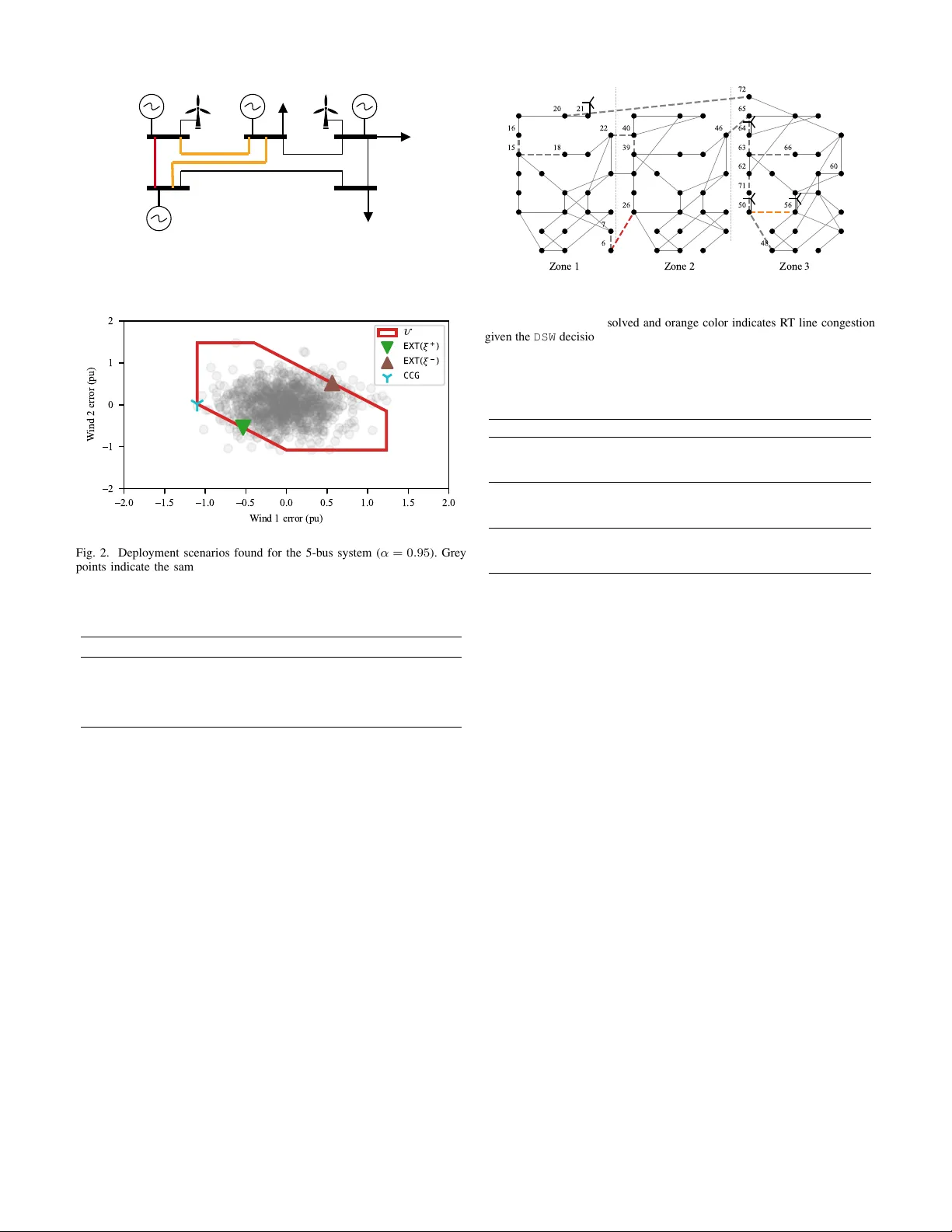
Constructing Deployment Scenarios for Reserv e Deli v erability via Adapti ve Rob ust Optimization Guillaume V an Caelenberg ∗ , Akylas Stratigak os † , Elina Spyrou ∗ ∗ Department of Electrical and Electronic Engineering, Imperial College London, U.K. † UCL Energy Institute, Uni versity College London, U.K. Abstract —Network congestion often hinders the deployment of r eserves needed to balance forecast errors during real-time operations. A pertinent idea to tackle this challenge in volves adding deployment scenarios of spatial distributions of forecast errors as contingencies to the day-ahead problem. However , current approaches disr egard the effect of grid topology and the day-ahead schedule on the induced congestion and, conse- quently , reser ve deliv erability . In this work, we formulate a two- stage adaptive robust optimization problem to jointly consider interactions between day-ahead and real-time operations and for ecast err ors. Using a column-and-constraint algorithm, we iteratively construct deployment scenarios by finding the worst- case f orecast error f or reser ve deliverability . Simulations on the R TS-GMLC system show that adding these scenarios to the day- ahead problem significantly r educes the frequency of congestion- driven reserve undeliverability . Notably , the choice and number of scenarios dynamically adapts to the day-ahead schedule. Index T erms —Electricity markets, operational uncertainty, probabilistic for ecasting, adaptive rob ust optimization, reserve deliverability. I . I N T R OD U C T I O N a) Backgr ound and Motivation: T o manage the growing imbalances between the day-ahead (D A) and real-time (R T) scheduling problems, partly caused by increasing variable renew able energy (VRE) forecast errors, system operators (SOs) reserve spare generation capacity in D A, which can be deployed in R T [1]. T o ensure that the frequency of reserve shortages remains below a prescribed reliability target, SOs are increasingly using probabilistic forecasts to determine the amount of required reserves dynamically [2]. T ypically , reserve requirements are estimated for the system as a whole or a limited number of large zones [3]. Ho wever , network conges- tion often renders reserves undeliv erable in R T . For instance, a significant portion of ramping reserve was undeliverable in 2018 in California [4]. b) Related W ork: Sev eral approaches of varying com- plexity could address the problem of undeliv erable reserves. At one end of the spectrum, computationally intensi ve for- mulations explicitly model the spatial distribution of forecast errors to obtain D A schedules that ensure the desired R T This work was funded by the Leverhulme International Professorship (LIP- 2020-002) and the Engineering and Physical Sciences Research Council under the grant EP/Y025946/1 (Electric Power Innovation for a Carbon-free Society (EPICS)). reliability [5]. For instance, two-stage stochastic optimiza- tion problems endogenously determine reserve capacity at various locations by minimizing probability-weighted costs ov er multiple scenarios with distinct spatial distributions of forecast errors. Howe ver , such methods may be impractical due to computational issues and lack of properties, desirable in markets [6]. As an alternati ve, robust optimization problems [7] ensure deliverability for all error realizations within a defined uncertainty set and closely resemble existing schedul- ing processes [8]. Howe ver , robust problems are sensitiv e to the design of the uncertainty set and often lead to overly conservati ve solutions. This conservati veness is to some extent reduced when robust problems are adaptiv e, considering multi- ple stages and allowing recourse actions at a later stage (e.g., R T redispatch) [9]. Solution approaches for adaptive robust problems usually assume a reserve activ ation policy [10] or iterativ ely find the worst-case realizations for a series of DA schedules [11]. Data-dri ven methods can be used to determine the parameters of reserve acti vation policies [12], [13]. At the other end, less computationally intensive methods rely on heuristics and approximations for generating D A schedules. While they aim for higher R T reliability than practices with network-unaware reserve procurement, they usually lack theoretical guarantees. For instance, reserving capacity at each node to meet nodal reserve needs is an inner approximation of the adaptiv e robust problem’ s feasible region that does not require any network capacity for reserves. In practice, imposing reserve requirements at ev ery node is often costly and sometimes impossible due to the lack of local reserv e suppliers. When reserve requirements are nodal, there are provisions for limited contribution of out-of-node resources. The limits on the contributions are determined through conserv ativ e approaches [14] or heuristics [15], [16]. Building upon the current practice of approximations with zonal reserve requirements, se veral articles propose a shift from zones with jurisdictional boundaries [17] to zones iden- tified based on active and reactiv e power flow analysis [18] and grid characteristics [19], [20]. T o account for dynamic congestion patterns, [21] presented a method for dynamically partitioning the grid into zones using probabilistic forecasts. More recently , SOs started incorporating forecast error scenarios as contingencies in their D A schedule to support reserve deli verability in R T [22], [23]; hereafter, we refer to them as deployment scenarios . By explicitly modeling R T redispatch actions under deployment scenarios, this approach advances the traditional deterministic modeling practice [24] and constitutes a second-best alternativ e to the optimal, but impractical, multi-stage stochastic and robust formulations. Howe ver , generating these deployment scenarios from prob- abilistic forecasts is an open question. Industry best practices typically account for a fe w extr eme scenarios with heuristically selected spatial distributions of forecast errors [25], potentially ov erlooking other possible distrib utions that could lead to reserve undeli verability due to unique grid characteristics. Importantly , these deployment scenarios are chosen without considering ho w reserve deliverability depends on the D A schedule and network congestion. c) Aim and Contribution: In this work, we develop a method for constructing deployment scenarios from a set of probabilistic forecasts, which are then included as con- tingencies in the DA scheduling problem. W e formulate a two-stage adaptive robust optimization (AR O) problem that jointly considers the D A schedule, worst-case forecast error realizations, and the full-recourse R T schedule. When the uncertainty set is polyhedral, the AR O problem is equiv alent to the standard D A scheduling problem with deployment scenarios as additional contingencies. Using the column-and- constraint (CCG) [26] algorithm, we construct deployment scenarios corresponding to a series of iterati vely updated D A schedules. W e apply this method to the R TS-GMLC 2019 [27] system and provide original insights into the differences between CCG-constructed deployment scenarios and extr eme deployment scenarios constructed following industry practice. W e find that CCG-constructed deployment scenarios often include errors in both directions (over - and under-forecasts) at dif ferent grid nodes, which contrasts extreme scenarios that include errors in a single direction. T o account for the aggre- gation benefits of forecast errors, extreme scenarios reduce the reserve requirement at each node based on a uniform across- nodes policy . In contrast, the CCG-constructed deployment scenarios allow the D A problem to endogenously calculate what level of aggregation benefit (if any) can be lev eraged, considering transmission constraints. Overall, our results show that incorporating deployment scenarios in the D A schedule improv es reserv e deli verability compared to network-una ware reserve procurement and that CCG-constructed deployment scenarios closely approximate prescribed reliability tar gets, while outperforming extreme scenario approaches. The rest of the paper is structured as follows. Section II presents the preliminaries on the reserve deli verability prob- lem. Section III describes our methodology proposed to con- struct deployment scenarios. Section IV presents the exper - imental design and results. Finally , Section V summarizes conclusions and provides directions for further research. I I . P R E L I M I N A R I E S In this section, we describe the operating framework (Sub- section II-A), and formulate the D A scheduling problem with deployment scenarios for the deliv erability of reserves as a two-stage AR O problem (Subsection II-B). Notation: W e use bold lowercase (uppercase) font for vectors (matrices) and calligraphic font for sets. Let | · | be the set cardinality and 1 be a vector of ones with appropriate size. Forecasts are denoted by ˆ ( · ) ; the v alue of decision variables at optimality is denoted by ˙ ( · ) . For a positiv e integer Q , we define [ Q ] = { 1 , . . . , Q } . A. Operating F rame work Consider a po wer system where N is the set of nodes, L is the set of lines, and G is the set of generators. For the i th period, the point forecast for the net demand (load minus VRE production) is ˆ d ∈ R |N | , and ξ ∈ R |N | is a random variable that describes the forecast error, defined as actual minus DA point forecast. The SO has access to a set E of K scenarios with forecast errors that account for spatial correlations, where E = { ˆ ξ k } k ∈ [ K ] . In practice, this information can be provided by methods that generate multiv ariate scenarios from marginal probabilistic forecasts using a Copula function — see, e.g., [28]. W e note the aggregate net demand error at the system lev el with ξ agg and compute its scenario-specific value, ˆ ξ agg k , as 1 ⊤ ˆ ξ k . For bre vity , the period index i is omitted. Consider a prescribed reliability lev el α ∈ (0 , 1) , where α is typically high, e.g., 0 . 90 , 0 . 95 . The system-wide reserve requirements for the i th period are estimated by ˆ ρ + = q 1+ α 2  { ˆ ξ agg k } k ∈ [ K ]  , ˆ ρ − = q 1 − α 2  { ˆ ξ agg k } k ∈ [ K ]  (1) where q u ( · ) is a function that takes as input K scenarios and returns the u th empirical quantile. In words, the likelihood of ξ agg being in the interval [ ˆ ρ − , ˆ ρ + ] is 100 · α % . T ypically , it holds that ˆ ρ − ≤ 0 and ˆ ρ + ≥ 0 , which implies that downw ard and upward reserves are procured to balance negativ e and positiv e errors of net demand, respectively . The SO solves two sequential optimization problems. In D A, the SO schedules energy and reserves. In R T , the SO adjusts the schedules to ensure cost-ef fective and reliable operations. As we are concerned with reserve undeliverability , the second stage objectiv e only considers reliability . 1 a) D A Problem: The DA (or first-stage) scheduling prob- lem is giv en by min p , r + , r − ( c e ) ⊤ p + ( c + ) ⊤ r + + ( c − ) ⊤ r − , (2a) s.t. 1 ⊤ p = 1 ⊤ ˆ d , (2b) 1 ⊤ r + ≥ ˆ ρ + , 1 ⊤ r − ≥ − ˆ ρ − , (2c) M ( Ap − ˆ d ) ≤ f max , (2d) − M ( Ap − ˆ d ) ≤ f max , (2e) p + r + ≤ p max , (2f) p − r − ≥ p min , (2g) p , r + , r − ≥ 0 . (2h) Problem (2) computes the least-cost energy ( p ∈ R |G | ) and re- serve schedule ( r + , r − ∈ R |G | ) (2a) to satisfy the net demand 1 T o highlight the article’s novel contributions, we solve a single-interval optimization problem. The core methodology can be extended for scheduling applications with commitment decisions and inter-temporal constraints. forecast (2b) and dynamic reserve requirements (2c), subject to transmission feasibility constraints (2d)-(2e) and constraints for minimum and maximum generating power (2f)-(2h). Here, ( c e , c + , c − ) represent linear costs, ( p max , p min , f max ) represent technical limits for energy and line flows, M ∈ R |L|×|N | is the Power Transfer Distribution Factors (PTDF) matrix, and A ∈ R |N |×|G | is the node incidence matrix that maps generators to nodes. b) RT Pr oblem: Giv en fixed first-stage decisions ˙ x = ( ˙ p , ˙ r + , ˙ r − ) and a realized net demand forecast error ξ 0 , the R T (or second-stage) redispatch problem that computes recourse actions p rec ∈ R |G | is giv en by min p rec , g + , g − , ℓ + , ℓ − ( c viol ) ⊤ ( g + + g − + ℓ + + ℓ − ) , (3a) s.t. 1 ⊤ p rec = 1 ⊤ ξ 0 , (3b) M ( Ap rec − ξ 0 ) ≤ f max − ˙ f e + ℓ + , (3c) − M ( Ap rec − ξ 0 ) ≤ f max + ˙ f e + ℓ − , (3d) p rec ≤ ˙ r + + g + , (3e) − p rec ≤ ˙ r − + g − , (3f) g + , g − , ℓ + , ℓ − ≥ 0 , (3g) where ˙ f e = M ( A ˙ p − ˆ d ) is shorthand for the D A scheduled energy flow . Note that the av ailable transmission capacity for recourse actions is f max − ˙ f e and f max + ˙ f e . Constraint (3b) ensures the R T balance of supply and demand. Constraints (3c)-(3d) and (3e)-(3f) ensure that recourse actions are within the generation reserved in DA and av ailable transmission capacity, respectiv ely . If the reserves are insufficient, e.g., R T schedules exceed capacities reserved in D A or cannot be deliv ered due to grid congestion, then the slack variables g − , g + ∈ R |G | and ℓ − , ℓ + ∈ R |L| become positive [29]. The objectiv e function (3a) imposes a large penalty c viol on non- zero slack values. B. Adaptive Robust Optimization F ormulation W e now formulate a two-stage AR O problem that enables reserve deliv erability and show that it can be equiv alent to (2) augmented with deployment scenarios. T o streamline notation, we rewrite problem (2) in a compact form as min x c ⊤ x , s.t. Bx ≤ b , where x = ( p , r + , r − ) , c = ( c e , c + , c − ) , and ( B , b ) parame- terize the set of linear inequalities 2 that represent the feasible set of (2). Next, we re write problem (3) as min p rec , s ≥ 0 ( c viol ) ⊤ s , s.t. H ˙ x + Dp rec − s ≤ E ξ 0 + h , where ˙ x are the fixed first-stage decisions, s = ( 0 , g + , g − , ℓ + , ℓ − ) , and ( H , D , E , h ) are constructed appropriately to represent the feasible set of (3). 3 2 Each equality constraint is replaced with two opposite inequalities. 3 In addition to slack variables, s includes 0 for the two opposite inequali- ties, replacing (3b). The two-stage AR O problem with full recourse, considering only feasibility penalties, is giv en by min x c ⊤ x + max ξ ∈U min p rec ( ξ ) , s ( ξ ) ( c viol ) ⊤ s ( ξ ) , (4a) s.t. Bx ≤ b , (4b) Hx + Dp rec ( ξ ) − s ( ξ ) ≤ E ξ + h , ∀ ξ ∈ U , (4c) s ( ξ ) ≥ 0 , ∀ ξ ∈ U , (4d) where second-stage decisions p rec ( ξ ) , s ( ξ ) are a function of ξ and U is an uncertainty set that cov ers potential realizations of net demand error ξ the system has to be reliable against. For example, U could coincide with E , or be a subset or an approximation of it. The choice of U is critical for both the performance guar- antees and the computational cost associated with solving (or approximating) (4). When U is a polyhedral or discrete set, then the worst-case cost occurs at one of its extreme points (vertices). Let V be a discrete set that contains all the vertices of U . Then, (4) is equi valent to min x , { p rec ξ , s ξ } ,η c ⊤ x + η , (5a) s.t. Bx ≤ b , (5b) η ≥ ( c viol ) ⊤ s ξ , ∀ ξ ∈ V , (5c) ( p rec ξ , s ξ ) ∈ Ω( x , ξ ) , ∀ ξ ∈ V , (5d) where η represents the worst-case violation cost, ( p rec ξ , s ξ ) are the wait-and-see second-stage decisions for each vertex in V , and Ω( x , ξ ) = { ( p rec , s ) : Hx + Dp rec ( ξ ) − s ( ξ ) ≤ E ξ + h , s ( ξ ) ≥ 0 } is the feasible set of the second-stage problem, given x , ξ . The objectiv e function (5a) consists of the DA scheduling cost and the worst-case violation cost. Note that (5d) includes the R T constraints for particular realizations of ξ , which could be interpreted as reserve deployment scenarios. Hence, the AR O formulation formally justifies the industry intuition of adding deployment scenarios to the DA problem. When (5d) is satisfied without slack activ ation for all vertices, η equals zero. If any slack is non-zero, then η is positiv e, and supply-demand balance is not guaranteed within U . In those cases, it is worth examining whether the system lacks reserves at the system level or at specific nodes and how accurate model inputs, such as U and c viol , are. The AR O reformulation shows that the success of the de- ployment scenarios hinges on the careful construction of these scenarios. The number of vertices in U may be exponential to the dimension of ξ , making verte x enumeration impractical for solving (5) to optimality . The next section presents two methods for constructing deployment scenarios from a set E of forecast error scenarios, which is one type of probabilistic forecast [30]. I I I . C O N S T RU C T I N G D E P L OY M E N T S C E N A R I O S In this section, we describe two methods for constructing deployment scenarios, assuming a polyhedral uncertainty set presented in Subsection III-A. First, we describe a method that only uses D A forecasts of net demand as inputs and resembles industry practices (Subsection III-B). Next, we de velop a method that additionally leverages grid characteristics and D A decisions, which comprise our key contribution (Subsec- tion III-C). A. Uncertainty Set In this work, and without a loss of generality, we assume that SOs aim to ensure reserve deliv erability when ξ agg lies within an interval bounded by the system-wide reserve re- quirements ˆ ρ + , ˆ ρ − , and is additionally bounded by nodal net demand errors lying within a “box”, giv en by U agg α = { ξ : ˆ ρ − ≤ 1 ⊤ ξ ≤ ˆ ρ + } , (6) U box = { ξ : min k ∈ [ K ] { ˆ ξ k } ≤ ξ ≤ max k ∈ [ K ] { ˆ ξ k }} , (7) where the box is bounded by the lowest and highest forecast error scenario (element-wise operation). The uncertainty set for problem (4) is giv en by the inter- section U = U agg α ∩ U box , which implies that U ⊆ U agg α and U ⊆ U box . In practice, SOs can also use other polyhedral uncertainty sets that may better reflect the distribution of forecast errors. The quality of uncertainty sets can be assessed in terms of cov erage, density , or interpretability . B. Extr eme Deployment Scenarios fr om F orecasts This approach resembles industry practice [25] and con- structs a set of two extreme deployment scenarios S depl : one for positiv e and one for ne gativ e forecast errors. This approach assumes that the most challenging case for reserve deliv erability is when all errors are in the same direction (positiv e or negati ve), which implies a high correlation among them. Here, we follow the same logic and distribute ˆ ρ + , ˆ ρ − to the nodes such that all errors are in the same direction. First, for the j th node, we calculate allocation factor e + j , which accounts for the 1+ α 2 -lev el marginal quantile forecasts as follows: e + j = q 1+ α 2  { ˆ ξ j,k } k ∈ [ K ]  P n ∈N q 1+ α 2  { ˆ ξ n,k } k ∈ [ K ]  . (8) In words, the allocation factors are proportional to the quan- tiles of nodal forecast errors. W e construct the upward deploy- ment scenario that includes in each node n an upward error equal to ξ + n = ˆ ρ + · e + n . An additional Euclidean projection step onto U is applied. W e follo w the same approach for the downw ard direction. C. Constructing Deployment Scenarios via CCG In this section, we construct deployment scenarios con- sidering their dependency on (i) problem parameters (e.g., grid topology) and (ii) first-stage decisions. W e apply a CCG algorithm [26] to iteratively add vertices, such that S depl ⊆ V . T o streamline notation, let Q ( ˙ x ) = max ξ ∈U min p rec ( ξ ) , s ( ξ ) ∈ Ω ( ˙ x , ξ ) ( c viol ) ⊤ s ( ξ ) (9) be the worst-case objectiv e value of the second-stage problem giv en fixed first-stage decisions ˙ x . The CCG algorithm is summarized in Algorithm 1. First, we consider an empty set of deployment scenarios, S depl , solve (5), and estimate a lower bound LB on the R T violation cost (lines 1, 3). Next, we fix the first-stage decisions and approximate the worst-case cost of the second stage Q ( ˙ x ) (line 4), which returns an approximately worst-case scenario ˜ ξ and an upper bound UB on the R T violation cost (line 5). If the worst-case scenario ˜ ξ has a non-zero violation cost, it is added to the set of deployment scenarios (lines 6-9). The algorithm terminates when UB = LB or when the maximum number of iterations M is reached. M can be chosen based on the number of deployment scenarios the SO can add to the D A schedule. If an oracle that optimally solves Q ( ˙ x j ) for a fixed ˙ x j is av ailable (step 4), then (5) is solved to optimality when Algo- rithm 1 con verges. In practice, ho wev er, computing Q ( ˙ x j ) is challenging because problem (9) is a nonconv ex max - min problem. Solution approaches reformulate the problem as a mixed-integer problem or rely on heuristics [26]. Here, we use the alternating dir ection method (ADM) heuristic to approximate Q ( ˙ x j ) (9), which has been sho wn to perform well in similar problems [31]. First, strong duality is applied to the inner min problem for a fixed ˙ x , reformulating the max - min problem into a max problem giv en by max π , ξ ∈U π ⊤ ( H ˙ x − E ξ − h ) , (10a) s.t. − D ⊤ π = 0 , (10b) 0 ≤ π ≤ c viol , (10c) where π denotes dual variables of the constraints in Ω( ˙ x , ξ ) . Second, Problem (10), which has a bilinear objecti ve, is solved via Algorithm 2. The algorithm relies on iterativ ely optimizing a relaxed linear program, where part of the decision v ariables are treated as constants (either π or ξ ). Giv en fixed first-stage decisions ˙ x and an initial guess ξ init , we maximize (10) over π (assuming ξ = ξ init ), which provides a lo wer bound LB Q (line 3). Then, we maximize (10) over ξ ∈ U , while π is fixed at the solution, which provides an upper bound UB Q (line 4). The local bounds are iterativ ely updated until con ver gence ( UB Q = LB Q ), which is then guaranteed to be a local optimum that satisfies the Karush–Kuhn–T ucker conditions [31], or the algorithm terminates when the maximum number of iterations L is reached. W e set ˜ Q ( ˙ x j ) as the average between UB Q , LB Q and return the worst-case scenario ξ wc = ξ l (line 7). The initial guess ξ init can be critical to the con vergence of Algorithm 2. Here, we dev elop a heuristic that chooses as initial guesses forecast error scenarios that could aggrav ate congestion. First, we select a set of lines that are sometimes congested in D A or R T when the solution of (2) is followed. Then, for each line l , we find the forecast error ξ that results in the highest power flow increase in the same direction as the D A flow ˙ f e l , obtained from (2), as follows max ξ ∈U box | ˙ f e l − M l ξ | . (11) Algorithm 1 Column-and-constraint Generation Input: Problem (5), maximum number of scenarios M . Output: S depl 1: Initialize S 0 = ∅ , UB = ∞ , LB = −∞ , j = 0 . 2: while UB − LB ≥ 0 and j ≤ M do 3: Solve (5) with V = S j and set ˙ x j = x ∗ , LB = η ∗ . 4: Approximate Q ( ˙ x j ) using ˜ Q ( ˙ x j ) . 5: Set ξ wc j = ˜ ξ , UB = ˜ Q ( ˙ x j ) . 6: if ˜ Q ( ˙ x j ) > 0 then 7: Update S j +1 = S j ∪ { ξ wc j } , j ← j + 1 . 8: end if 9: end while 10: Return S depl = S j . Algorithm 2 Alternating Direction Method Input: First-stage decisions ˙ x , maximum number of iterations L , initialization ξ init . Output: ˜ Q ( ˙ x ) , ˜ ξ 1: Initialize by UB Q = ∞ , LB Q = −∞ , l = 0 , ξ l = ξ init . 2: while UB Q − LB Q ≥ ϵ and l ≤ L do 3: Solve max 0 ≤ π ≤ c viol π ⊤ ( H ˙ x − E ξ − h ) , s.t. − D ⊤ π = 0 , set π l = π ∗ , update LB Q . 4: Solve max ξ ∈U π ⊤ l ( H ˙ x − E ξ − h ) , update UB Q . 5: l → l + 1 6: end while 7: Return ˜ Q ( ˙ x ) = UB Q + LB Q 2 , ˜ ξ ← ξ l . (11) admits a closed-form solution (note that ˙ f e l is fixed), which is a verte x of U box . The verte x includes, for each node j , the maximum nodal forecast error , when term ( sign ( ˙ f e l ) · M l,j ) is negativ e; and the minimum nodal forecast error when the same term is positive. This v ertex is then projected onto U to obtain an initial guess. In addition, we use the two extreme deployment scenarios from Subsection III-B as initializations ξ init . That way , the use of the CCG-constructed scenarios will result in a le vel of reliability at least as good as the one achieved by using the extreme scenarios. Out of all initializations, we pick the scenario ξ wc that leads to the highest ˜ Q ( ˙ x j ) . The computational ov erhead of the CCG algorithm is antic- ipated to be similar to that of other iterative solutions currently implemented by system operators [32]. Note that Algorithm 2 can be trivially parallelized for multiple initializations. I V . N U M E R I C A L E X P E R I M E N T S A N D R E S U LT S In this section, we summarize the experimental design (Subsection IV -A), discuss an illustrati ve example (Subsection IV -B) and analyze results for annual simulations of the R TS- GMLC 2019 system (Subsection IV -C). A. Experimental Design For a given reliability level α , we contrast three approaches: (i) DSW , where we solve (2) with system-wide reserve require- ments estimated from (1); (ii) EXT , where we solve (5) with two extreme deployment scenarios constructed with method shown in Subsection III-B; and (iii) CCG , where we solve (5) with deployment scenarios constructed by applying CCG, as shown in III-C, for U = U agg α ∩ U box . B. Illustrative Example W e first discuss results for a modified IEEE 5-bus system [33]. The results can be easily verified by the reader and provide intuition for appreciating the results for the larger system in the next section. The system has two wind power plants, shown in Fig. 1. W ind plant 1 is located in node 3 alongside the cheapest generator, whereas wind plant 2 is located in node 5 alongside the most expensi ve generator . W e consider wind forecast errors following a zero-mean multiv ariate normal distribution, where Σ =  0 . 141 0 . 001 0 . 001 0 . 141  (pu) 2 , is the cov ariance matrix. W e sample K = 1 000 DA sce- nario forecasts for ˆ ξ k , calculate the system-wide require- ments ˆ ρ + , ˆ ρ − for α = 0 . 95 , and construct two sets of deployment scenarios using EXT and CCG . T o assess out-of- sample performance, we sample an additional 1 000 scenarios (representing realized errors), and solve the R T problem (3), for c viol = 1 000 $/MWh. In addition to DSW , EXT , and CCG , we solv e (5) to optimality via vertex enumeration ( V-enum ). Fig. 2 plots the uncertainty set U , which is enclosed by the red curve, and the respective deployment scenarios. CCG terminates after adding a single scenario, ξ wc 1 , located at the bottom left verte x, to the D A problem whereas EXT adds two deployment scenarios, and V-enum adds all six extreme points shown in Fig. 2. T able I presents the average results for scenarios with realized error that belongs to U . Both EXT and CCG lead to higher D A costs and lower R T penalties compared to DSW . For EXT , 3 . 3% of out-of-sample observ ations within U violate R T constraints (i.e., hav e at least one R T slack variable with non-zero value). This is an order of magnitude lower than the 54 . 4% obtained under DSW . CCG performs best in terms of reliability , with 0% violations. In this case, CCG found the same solution as V-enum , while only using a single scenario. Examining the DA decisions obtained by DSW , we observe that the generator at node 5 is the sole reserve supplier, line 1 - 5 is congested, and lines 1 - 4 , 4 - 5 are close to becoming congested. When upward reserves are needed due to negati ve errors in the wind plant 1 (over -forecast of wind production), the orange lines shown in Fig. 1 become congested and the reserves procured at node 5 cannot be deli vered. The EXT deployment scenario ξ + accounts for the impact of constraints on reserve deliverability , but does not consider the worst- case of forecast errors in wind plant 1 as the grid is ignored during scenario construction. In contrast, the CCG deployment scenario ξ wc 1 fully mitigates reserve undeliverability within the uncertainty set U . In the D A solution deriv ed by CCG , the more expensi ve generator at node 3 provides some reserves to compensate for the potential forecast errors in wind plant 1 , while energy schedule remains unchanged. While, in this 1 5 4 3 2 W ind 1 W ind 2 Fig. 1. Schematic of the 5-bus system. Red color indicates line congestion in D A DSW schedule. Orange color indicates R T line congestion given the DSW decisions, causing deliv erability problems.                         E X T ( + ) E X T ( ) C C G Fig. 2. Deployment scenarios found for the 5-bus system ( α = 0 . 95 ). Grey points indicate the sampled scenarios, used to construct the uncertainty set. T ABLE I R E SU LT S F O R T H E 5 - BU S S Y S T EM ( α = 0 . 95 ) . D A cost ( 10 3 $/h) A v . R T cost ( 10 3 $/h) V iol. Prob . (%) DSW 131 134 54.4 EXT 140 1 3.3 CCG 142 0 0 V-enum 142 0 0 example, the DA schedule changed only in terms of reserve schedules, we will see in the next section that inclusion of deployment scenarios in D A can lead to changes in the energy schedule and the av ailable transmission capacity for recourse actions. C. RTS-GMLC 2019 System a) System Information: The R TS-GMLC 2019 System [27] has 73 buses, 120 transmission lines, 73 con ventional generators, 4 wind power plants, and 56 solar power plants, organized in 3 zones (Fig. 3). W e assume perfect demand forecasts and consider imperfect forecasts for the 60 VRE plants. W e use time series data provided by [34] and prob- abilistic forecasts provided by [28], comprising K = 500 scenarios. The data set cov ers a full year at hourly granularity . Exploratory data analysis indicated that the 4 wind plants at nodes 21 , 50 , 56 , and 64 , and the solar plant at node 60 account for approximately 75% of the total forecast errors in terms of absolute magnitude.                               Fig. 3. Grid topology of R TS-GMLC 2019 System. Red color indicates line congestion after DSW is solved and orange color indicates R T line congestion giv en the DSW decisions, for the illustrative period. Bold dashed lines are used to initialize ADM. T ABLE II R E SU LT S F O R A S I M U LAT IO N Y E AR F O R T H E RT S -G M L C S Y S TE M . A v . D A cost (10 3 $ / h ) A v . R T cost (10 3 $ / h ) V iol. Prob . (%) α = 0 . 90 DSW 64.57 10.69 16.96 EXT 65.65 1.00 2.92 CCG 78.31 0.02 0.08 α = 0 . 95 DSW 68.24 11.20 16.92 EXT 69.66 0.94 2.40 CCG 82.51 0.01 0.15 α = 0 . 99 DSW 75.91 12.00 17.14 EXT 78.53 0.51 2.56 CCG 90.26 0.06 0.55 b) Implementation Hyper-parameter s: W e compare DSW , EXT , and CCG for le vels of α = { 0 . 90 , 0 . 95 , 0 . 99 } , and use a high violation penalty of c viol = 1 000 $/MWh. For the D A scheduling problem (2), we also include an additional variable that allows for VRE curtailment, bounded by the respectiv e point forecast. For CCG , we run the alternating direction method with L = 20 , which is nev er reached, and set the maximum number of scenarios for each period at M = 10 . W e initialize Algorithm 2 with the extreme scenarios deriv ed for EXT and with scenarios found using (11) for 15 lines that are sometimes congested in D A or R T , according to the DSW - based results — see Fig. 3 for a visualization of the selected lines. c) Annual P erformance: T able II presents annual aver - ages for performance metrics under the different approaches, for α = { 0 . 90 , 0 . 95 , 0 . 99 } . The metrics are reported for hours with realized R T error falling within the respectiv e U . The percentage of observ ations falling in U for each experiment is approximately 71% for α = 0 . 90 ; 76% for α = 0 . 95 ; and 82% for α = 0 . 99 . This undercoverage is attributed to the quality of the probabilistic forecasts, which are an exogenous input in this work. From T able II, as α increases, the D A cost increases and R T cost decreases for all methods, which is expected as the reserve requirements increase with α . DSW , as expected, performs worst in terms of reliability , with an av erage violation frequency of approximately 17% for all α , b ut performs best in terms of DA cost. Considering that we report the frequency of             E X T  + E X T  C C G  w c 1 C C G  w c 2 Fig. 4. Deployment scenarios for EXT and CCG for the illustrative period. Dashed lines indicate ˆ ρ + , ˆ ρ − . The × marker indicates realized errors. violations when the realized error falls in U , we would expect a fully reliable method to hav e a frequency of violations close to 0 , i.e., assuming (4) is solved to optimality . Indeed, CCG achiev es a violation frequency ≤ 1% in all cases, whereas EXT is second-best in terms of reliability . T o understand why these few R T violations within U persist, we examine whether the D A schedule is feasible without using any slack v ariables (i.e., η ∗ = 0 ). For instance, for α = 0 . 95 , 10 simulated hours hav e non-zero R T penalty cost and belong to U . Among these 10 hours, 8 hours hav e η ∗ = 0 4 . The R T violations during these hours indicate that the ADM failed to find the worst-case error scenario. Whereas CCG does not provide any guarantees about relia- bility outside U , the results are similar to the ones inside U , with CCG leading to a lower violation frequency and higher D A costs compared to EXT . For example, for α = 0 . 95 , the actual error is outside U for 24% of the hours. Over these hours, EXT and CCG hav e an av erage D A cost of 66 . 85 and 80 . 99 10 3 $ / h, respectiv ely; while they record R T violations for 52 . 11% and 39 . 65% of the hours, respectiv ely . The CCG achiev es better performance in terms of reliability by adjusting the choice and number of vertices added as deployment scenarios, considering the dynamic congestion patterns. For instance, for α = 0 . 95 , CCG recovers 3 or more deployment scenarios in approximately 36% of the time. Lastly , it is worth noting that while EXT procures the same amount of upward and do wnward reserve as DSW , this is not the case for CCG which might choose to procure additional reserve due to congestion anticipated in deployment scenarios with spatial distribution of forecast errors dif ferent than EXT . For α = 0 . 95 , in respectiv ely 10 . 9% and 20 . 8% of the hours CCG procures more up or do wn reserv e than DSW , which implies that the full aggregation benefit cannot be le veraged due to transmission constraints. For these hours, on av erage 3 . 6 deployment scenarios are included in the D A schedule. d) Impact of Initialization: W e examine the sensitivity of the CCG algorithm w .r .t. the starting points by running it 4 T wo hours have η ∗ > 0 , which either indicates that c viol is low or that there is no feasible DA schedule that guarantees zero constraint violations in U . In practice, for such cases, the operator can increase the value of c viol . with an alternative set of starting points, including only the extreme scenarios. This results for α = 0 . 90 / 0 . 95 / 0 . 99 in a violation probability in U of 1 . 34 / 1 . 36 / 1 . 48% , which is better than EXT and worse than the results in T able II, which chose starting points based on the initialization strategy of (11). e) Illustrative P eriod: W e illustrate ho w CCG constructs better deployment scenarios by examining a particular hour (with α = 0 . 90 ) for which the actual error realization falls inside U and EXT leads to deliverability issues (i.e., non- zero R T penalty), while CCG does not. For the selected hour, the only VRE generating electricity is wind; Fig. 4 plots the deployment scenarios of EXT and CCG alongside the system- wide requirements ˆ ρ + , ˆ ρ − and the realized error , showing only nodes 21 , 50 , 56 and 64 , corresponding to the four wind plants. For both EXT and CCG , the aggre gate error in each deployment scenario is equal to either ˆ ρ + or ˆ ρ − , but its distribution among nodes differs. EXT distributes the nodal errors proportionally to the width of the prediction interval of nodal VRE output. For CCG , the first deployment scenario, ξ wc 1 , has an aggregate error equal to ˆ ρ − ; compared to ξ − , ξ wc 1 leads to a much higher allocation in nodes 50 , 64 (R T wind production higher than forecasted) whereas nodes 21 , 56 hav e a smaller error with opposite sign; thus, ξ wc 1 represents a less correlated setting. Concerning the second deployment scenario, ξ wc 2 , we observe that all nodal errors are positiv e (R T wind production lower than forecasted) with the aggre gate error equal to ˆ ρ + ; and the allocation is not proportional to the width of the prediction interval at each node, with relati vely to EXT a higher allocation at nodes 50 , 64 . The line connecting nodes 6 - 26 is congested in the DSW solution of the D A problem. In R T , a large negati ve error (R T wind production higher than forecasted) occurs in node 50 (see × marker in Fig. 4); in turn, under DSW , the re-dispatch causes congestion in line 50 - 56 and leads to activ ating the respectiv e slack variable (approximately 96 MW); the same slack is activ ated in R T for EXT but at a lower le vel than in DSW ( 47 MW), meaning that EXT only partially resolves the deli verability issue. In contrast, CCG does not activ ate any slacks in R T . T o understand this effect, we e xamine the aggre gate energy and reserve schedule illustrated in Fig. 5. Firstly , CCG schedules more energy in zone 2 by curtailing a portion of wind production in node 50 , thus creating av ailable transmission capacity for recourse actions of 187 MW in line 50 - 56 , which is higher than the 97 MW created by EXT . Secondly , CCG shifts upward reserve schedule from zone 1 and 2 to zone 3, whereas downw ard reserves shift from zone 3 to zone 1 and 2, which is due to the fact that the deployment scenarios consider higher negati ve forecast errors in nodes 50 , 64 . This can also be understood from the sign of the respecti ve entries within the PTDF matrix, which are negati ve for nodes 50 , 64 tow ards line 50 − 56 and thus the second CCG -scenario creates bigger av ailable transmission capacity for recourse actions than EXT . The rest of the time periods offer similar insights. Namely , the CCG deployment scenarios allocate the uncertainty non- proportionally across nodes. As a result, CCG yields adapted energy-reserv e schedules and av ailable transmission capacity                       Fig. 5. DA schedule for a selected period, aggregated per zones. for recourse actions, fit for balancing dif ferent spatial distri- butions of forecast errors. V . C O N C L U S I O N T ransmission congestion often renders reserves undeliv er- able during real-time operations, threatening system reliability . Emerging industry practices add a set of deployment scenarios as contingencies to the day-ahead scheduling problem to en- hance reserve deliv erability during real-time operations. Ho w- ev er, industry practices for constructing deployment scenarios typically ignore the interdependency between deployment sce- narios, grid topology , and day-ahead schedules. In this work, we lev erage adaptiv e robust optimization to formulate a two- stage problem that jointly considers the day-ahead schedule and worst-case scenarios for reserve deliverability , and solve it via a column-and-constraint algorithm to generate reserve deployment scenarios. W e conduct simulations for the R TS- GMLC 2019 system using two sets of scenarios: one set is constructed via the CCG algorithm and another based on a method that resembles current industry practice Overall, the deployment scenarios constructed via the CCG algorithm significantly lower the number of hours with undeliverable re- serves and are more appropriate to meet the system operator’ s reliability targets. Contrary to prev ailing industry heuristics, these deployment scenarios often include forecast errors in opposite directions, which ha ve the effect of aggrav ating the congestion of transmission lines. In addition, simulation results show that the number of deployment scenarios and the spatial distributions of errors dynamically adapt to the day- ahead conditions. Future work could quantify the benefits of the proposed approach for scheduling processes that include commitment decisions and inter-temporal constraints. Further work could expand the CCG algorithm to include provisions for cases where no feasible day-ahead schedule is found to be robust within the uncertainty set. Alternative algorithms for solving the adversarial problem could also be tested. Lastly , it is interesting to examine generating deployment scenarios directly from data, thus bypassing the need for iterativ e solution techniques. R E F E R E N C E S [1] FERC Staff Paper, “Energy and ancillary services market reforms to ad- dress changing system needs, ” Federal Energy Regulatory Commission (FERC), Docket NO. AD21-10-000, 2021. [2] K. De V os, N. Stevens, O. Dev older , A. Papav asiliou, B. Hebb, A, and J. Matthys-Donnadieu, “Dynamic dimensioning approach for operating reserves: Proof of concept in Belgium, ” Energy P olicy , vol. 124, pp. 272–285, 2019. [3] E. Ela, R. Hytowitz, and U. Helman, ”Ancillary services in the United States: Technical requirements, market designs and price trends”, EPRI, Palo Alto, CA, T ech. Rep. 3002015670, 2019. [4] California Independent System Operator, “Refresher training: Flexible ramping product (FRP) refinements – Deliverability , ” 2022. [5] L. A. Roald, D. Pozo, A. Papa vasiliou, D. K. Molzahn, J. Kazempour, and A. Conejo, “Power systems optimization under uncertainty: A revie w of methods and applications, ” Electr . P ow . Syst. Res. , vol. 214, 2023. [6] J. Kazempour, P . Pinson, and B. F . Hobbs, “ A stochastic market design with rev enue adequacy and cost recovery by scenario: Benefits and costs, ” IEEE T rans. P ower Syst. , vol. 33, no. 4, pp. 3531–3545, 2018. [7] D. Bertsimas and D. den Hertog, Robust and adaptive optimization . Dynamic Ideas LLC, 2020. [8] A. Street, A. Moreira, J. M. Arroyo, N. Alguacil, and L. Barroso, “Robustness: The missing ingredient in generation scheduling, ” IEEE P ower and Ener gy Magazine , vol. 23, no. 3, pp. 31–43, 2025. [9] D. Bertsimas, E. Litvinov , X. A. Sun, J. Zhao, and T . Zheng, “ Adap- tiv e robust optimization for the security constrained unit commitment problem, ” IEEE T rans. P ower Syst. , vol. 28, no. 1, pp. 52–63, 2012. [10] D. Bertsimas and A. G. Koulouras, “Marginal pricing in adaptiv e robust unit commitment under load and capacity uncertainty , ” IEEE T rans. P ower Syst. , vol. 40, no. 1, pp. 341–354, 2025. [11] P . Donti, A. Agarwal, N. V . Bedmutha, L. Pileggi, and Z. J. K olter , “ Adversarially robust learning for security-constrained optimal power flow , ” 34th Adv . in Neural Information Processing Systems , 2021. [12] J. D. Lyon, M. Zhang, and K. W . Hedman, “Locational reserve disqual- ification for distinct scenarios, ” IEEE T rans. P ower Syst. , vol. 30, no. 1, pp. 357–364, 2015. [13] N. G. Singhal, N. Li, and K. W . Hedman, “ A data-driven reserve response set policy for power systems with stochastic resources, ” IEEE T rans. Sustain. Energy , vol. 10, no. 2, pp. 693–705, 2019. [14] M. Madani, A. Papav asiliou, and Z. Ruan, “The inscribed boxes ap- proach to reserve deliverability in balancing capacity markets: Base results, ” 21st Int. Conference on European Energy Market , 2025. [15] Z. Liang, R. Mieth, Y . Dvorkin, and M. A. Ortega-V azquez, “W eather- Driv en flexibility reserve procurement: A NYISO offshore wind power case study, ” , 2022. [16] K. V an den Bergh, K. Bruninx, and E. Delarue, “Cross-border reserve markets: network constraints in cross-border reserve procurement, ” En- er gy P olicy , vol. 113, pp. 193–205, 2018. [17] L. Meeus, The Evolution of Electricity Markets in Eur ope . Edward Elgar , 2020. [18] A. Kumar , S. Srivasta va, and S. Singh, “ A zonal congestion management approach using real and reactive power rescheduling, ” IEEE T rans. P ower Syst. , vol. 19, no. 1, pp. 554–562, 2004. [19] F . W ang and K. W . Hedman, “Dynamic reserve zones for day-ahead unit commitment with renewable resources, ” IEEE T rans. P ower Syst. , vol. 30, no. 2, pp. 612–620, 2015. [20] M. Xu, C. J. Dent, and A. W ilson, “Zonal operating reserv e demand curve applied to day-ahead deterministic unit commitment, ” Int. Conf. on Pr obabilistic Methods Applied to P ower Systems , 2016. [21] N. Viafora, S. Delikaraoglou, P . Pinson, G. Hug, and J. Holbøll, “Dy- namic reserve and transmission capacity allocation in wind-dominated power systems, ” IEEE T rans. P ower Syst. , vol. 36, no. 4, pp. 3017–3028, 2021. [22] G. Angelidis, “Flexible ramp product refinements: Appendix B. Pro- curement and deployment scenarios draft technical description, ” 2020. [23] Y . Chen, “ Addressing uncertainties through improved reserve product design, ” IEEE T rans. P ower Syst. , vol. 38, no. 4, pp. 3911–3923, 2023. [24] B. F . Hobbs, V . Krishnan, J. Zhang, H. F . Hamann, C. Siebenschuh, R. Zhang et al. , “How can probabilistic solar power forecasts be used to lower costs and improve reliability in power spot markets? A revie w and application to flexiramp requirements, ” IEEE Open Access Journal of P ower and Ener gy , vol. 9, pp. 437–450, 2022. [25] California Independent System Operator , “Business requirements spec- ification: Day-ahead market enhancements, ” 2023. [26] B. Zeng and L. Zhao, “Solving two-stage robust optimization problems using a column-and-constraint generation method, ” Oper . Res. Letters , vol. 41, no. 5, pp. 457–461, 2013. [27] Reliability T est System - Grid Modernization Lab Consortium. [Online]. A vailable: https://github.com/GridMod/R TS- GMLC [28] R. Carmona and X. Y ang, “Joint granular model for load, solar and wind power scenario generation, ” IEEE T rans. Sustain. Energy , vol. 15, no. 1, pp. 674–686, 2024. [29] F . W ang and Y . Chen, “Market implications of short-term reserve deliv erability enhancement, ” IEEE T rans. P ower Syst. , vol. 36, no. 2, pp. 1504–1514, 2020. [30] S. E. Haupt, M. Garcia Casado, M. Davidson, J. Dobschinski, P . Du, M. Lange, T . Miller , C. Mohrlen, A. Motley , R. Pestana, and J. Zack, “The use of probabilistic forecasts: Applying them in theory and practice, ” IEEE P ower and Ener gy Magazine , vol. 17, no. 6, pp. 46– 57, 2019. [31] A. Lorca and X. A. Sun, “ Adaptiv e robust optimization with dynamic uncertainty sets for multi-period economic dispatch under significant wind, ” IEEE T rans. P ower Syst. , vol. 30, no. 4, pp. 1702–1713, 2014. [32] Y . Chen, F . Pan, F . Qiu, A. S. Xavier , T . Zheng, and M. Marwali, “Security-constrained unit commitment for electricity market: Modeling, solution methods, and future challenges, ” IEEE Tr ans. P ower Syst. , vol. 38, no. 5, pp. 4668–4681, 2023. [33] R. Mieth and H. V . Poor, “Prescribed robustness in optimal power flow , ” Electr . P ow . Syst. Res. , vol. 235, p. 110704, 2024. [34] B. Sergi, C. Feng, F . Zhang, B.-M. Hodge, R. Ring-Jarvi, R. Bryce, K. Doubleday , M. Rose, G. Buster, and M. Rossol, “ Arpa-e perform datasets, ” Open Energy Data Initiative (OEDI), National Renewable Energy Laboratory (NREL), https://doi.org/10.25984/1891136, 2022, accessed: 2026-02-28. [Online]. A v ailable: https : // data .openei . or g / submissions/5772