GeMA: Learning Latent Manifold Frontiers for Benchmarking Complex Systems

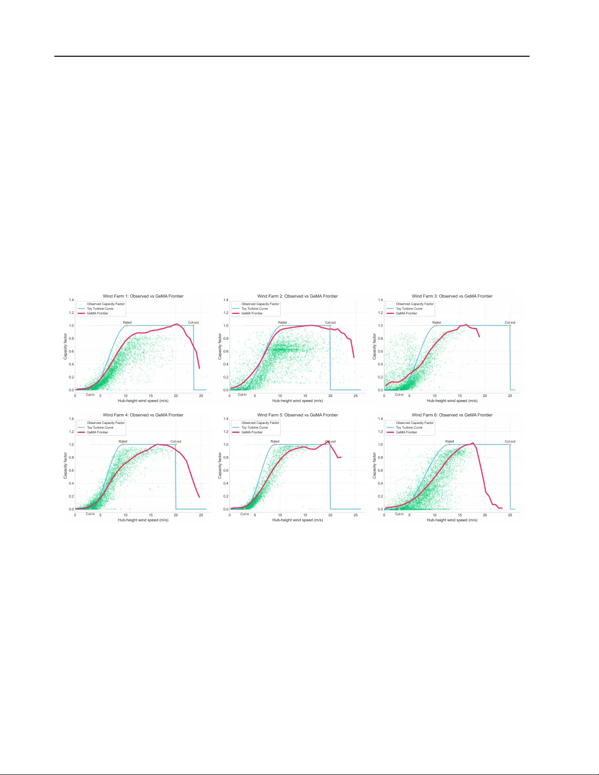
GeMA: Learning Latent Manif old Fr ontiers f or Benchmarking Complex Systems Jia Ming Li Anupriya Daniel J. Graham Abstract Benchmarking the performance of comple x sys- tems such as urban and national rail networks, re- ne wable generation assets and national economies is an important component of transport planning, regulation and macroeconomic analysis. Classical frontier methods, in particular Data Env elopment Analysis (DEA) and Stochastic Frontier Analy- sis (SF A), estimate an ef ﬁcient frontier in the ob- served input–output space and deﬁne efﬁcienc y as distance to this frontier . While empirically useful, these approaches often rely on restrictive assump- tions on the production possibility set, con vex- ity , separability or speciﬁc parametric functional forms, and address structural heterogeneity and scale effects only indirectly . W e propose Geometric Manifold Analysis ( G E M A ), a latent manifold frontier framework implemented via a productivity-manifold varia- tional autoencoder (P R O M A N - V A E). Instead of specifying a frontier function in the observed space, G E M A represents the production set as the boundary of a low-dimensional manifold embed- ded in the joint input–output space. A split-head encoder learns disentangled latent v ariables that capture technological structure and operational inefﬁcienc y . Ef ﬁciency is e valuated with respect to the learned manifold; endogenous peer groups arise as clusters in latent technology space; a quo- tient construction supports scale-in variant bench- marking; and a local certiﬁcation radius, deri ved from the decoder Jacobian and a Lipschitz bound, quantiﬁes the geometric robustness of indi vidual efﬁcienc y scores. W e validate the frame work on synthetic data de- signed to exhibit non-con ve x frontiers, heteroge- neous technologies and scale bias, and on four real-world case studies: global urban rail sys- T ransport Strategy Centre, Imperial Colle ge London, London, SW7 2AZ, United Kingdom. Correspondence to: Jia Ming (Simon) Li < jiaming.li@imperial.ac.uk > . Pr eprint. Marc h 18, 2026. tems (COMET), British rail operators (ORR), na- tional economies (Penn W orld T able) and a high- frequency wind f arm dataset (WF). Across these domains G E M A behav es comparably to estab- lished methods when classical assumptions are approximately satisﬁed, and it appears to provide additional insight in settings with pronounced het- erogeneity , non-con vexity or size-related bias. W e conclude by outlining how the static framew ork may be extended to a dynamic latent state-space “world model” of complex production systems, opening a path to wards counterfactual analysis and policy design on the learned manifold. Keyw ords: Latent variable models, Deep generati ve mod- els, Manifold learning, Frontier estimation, Efﬁcienc y anal- ysis. 1. Introduction Benchmarking the performance of complex systems is a widely used instrument in gov ernance, regulation and strate- gic planning. Urban and national rail networks, rene wable energy assets and national economies are routinely com- pared using efﬁcienc y scores deriv ed from frontier methods. Conceptually , the task is to estimate an ef ﬁcient frontier describing the best attainable outputs for gi ven inputs, and to quantify how far each decision-making unit (DMU) lies from this frontier . T wo main families of methods hav e been particularly in- ﬂuential in this ﬁeld. Stochastic Frontier Analysis (SF A) speciﬁes a parametric production function with a composed error term that separates noise and inef ﬁciency ( Aigner et al. , 1977 ; Meeusen & van Den Broeck , 1977 ; Greene , 1993 ; Sickles & Zelenyuk , 2019 ). Data En velopment Analysis (DEA) constructs a piecewise-linear efﬁcient frontier en- veloping the data via linear programming ( Charnes et al. , 1978 ; Coelli et al. , 2005 ). Both approaches hav e been widely applied in transport, energy , health and macroeconomic ap- plications (e.g. Oum et al. , 1999 ; Graham , 2008 ; Simar & W ilson , 2015 ) and have become standard tools in re gulatory benchmarking ( Smith , 2005 ; Rostamzadeh et al. , 2021 ). 1 Submission and Formatting Instructions f or ICML 2026 Howe ver , contemporary datasets pose sev eral structural chal- lenges. First, hetero geneity : DMUs may operate under markedly dif ferent technological or or ganisational regimes, so that a single global frontier is dif ﬁcult to interpret and may systematically fav our some groups o ver others. Secondly , non-con vexity and non-linearity : indivisible in vestments, network ef fects and physical constraints can lead to produc- tion sets that are not well approximated by con vex hulls or simple parametric forms ( K eshv ari & Kuosmanen , 2013 ). Thirdly , scale bias : in macroeconomic and infrastructure datasets, larger entities often receiv e higher efﬁciency scores simply because of their absolute size, e ven after controlling for standard inputs. Finally , there is a trust question: ef- ﬁciency scores are commonly reported as point estimates, with limited information on their stability to small perturba- tions in data or model speciﬁcation. Recent work has sought to relax some of the structural assumptions in classical frontier analysis. Con vex non- parametric least squares (CNLS) and related approaches reinterpret DEA as a conv ex regression problem and im- pose shape constraints via inequalities on regression coef- ﬁcients ( Daraio & Simar , 2006 ; Kuosmanen & Johnson , 2010 ). Stochastic non-con ve x en velopment and order- m frontiers explore non-con ve x production sets and robustness to extreme points ( Simar , 2007 ; Keshv ari & Kuosmanen , 2013 ). In parallel, machine learning methods ha ve been used to estimate production functions with greater ﬂe xibil- ity , employing kernel methods, tree ensembles and neural networks ( Breiman , 2001 ; Chen & Guestrin , 2016 ; Good- fellow et al. , 2016 ). Deep learning has also been brought into efﬁcienc y analysis, both for predicting outputs and for re-ev aluating DEA benchmarks ( Bose & Patel , 2015 ; Guer- rero et al. , 2022 ; Tsionas et al. , 2023 ). These developments, whilst valuable, typically retain the vie w of the frontier as a function in the observed input–output space and do not fully exploit the potential of latent v ariable modelling. In this paper , we take a complementary perspecti ve. Build- ing on the manifold hypothesis in representation learning ( Bengio et al. , 2013 ) and ideas from geometric deep learn- ing ( Bronstein et al. , 2017 ; 2021 ), we model the production possibility set as a low-dimensional, non-linear manifold embedded in the joint input–output space, and treat the fron- tier as the Pareto boundary of the production set induced by a latent v ariable model. W e introduce Geometric Manifold Analysis (G E M A ), implemented by a producti vity-manifold variational autoencoder ( P RO M A N - V A E ), which learns a latent technology coordinate and a separate inef ﬁciency fac- tor from data. This construction enables us to represent ﬂexible, potentially non-con vex frontiers, accommodate het- erogeneous technologies as distinct re gions of a shared man- ifold, deﬁne a quotient manifold that reduces certain scale effects, and attach a simple geometric robustness score to each efﬁcienc y estimate. Building on these ideas, our contributions are as follo ws: • W e introduce Geometric Manifold Analysis ( G E M A), a latent-manifold frontier framew ork in which the pro- duction possibility set is deﬁned as the image of a lo w- dimensional manifold in joint input–output space. The associated P RO M A N - V A E model disentangles latent technology from inefﬁciency under basic economic shape constraints, yielding a generativ e SF A-style for- mulation with explicit production-set semantics. • W e propose two geometric diagnostics for ef ﬁciency analysis: (i) a quotient construction that supports scale- in variant benchmarking by factoring out joint rescal- ings of inputs and outputs, and (ii) a local certiﬁcation radius deri ved from the decoder Jacobian, which pro- vides an interpretable indicator of the local robustness of efﬁcienc y scores. • W e empirically study G E M A on synthetic data and three complex domains: national rail operators (ORR), a high-frequency wind farm dataset (WF) and macroe- conomic data (PWT), with an additional urban rail case (COMET) in the appendix. The experiments show that G E M A behav es comparably to classical frontier esti- mators when their assumptions are approximately sat- isﬁed, and can offer additional insight in settings with non-con vex technologies, unobserv ed heterogeneity or scale-related bias. The remainder of the paper is organised as follows. Sec- tion 2 brieﬂy re vie ws related w ork in frontier analysis, latent variable models and geometric deep learning. Section 3 in- troduces the G E M A framew ork and the P RO M A N - V A E architecture. Section 4 presents synthetic experiments and case studies on wind farms, national rail operators and macroeconomic data. Section 5 discusses implications and limitations, and Section 6 concludes. Detailed deri vations, additional experiments and data descriptions are provided in the appendices. 2. Related W ork Frontier and efﬁciency analysis. Classical efﬁcienc y analysis b uilds on the notion of a production set and its efﬁcient frontier ( F arrell , 1957 ). Stochastic Frontier Analy- sis (SF A) speciﬁes a parametric production function, often Cobb–Douglas or T ranslog, with a composed error term that separates statistical noise from a one-sided inefﬁcienc y com- ponent ( Aigner et al. , 1977 ; Meeusen & van Den Broeck , 1977 ; Greene , 1993 ; Sickles & Zelenyuk , 2019 ). This econo- metric approach supports statistical inference and panel extensions, b ut is sensitive to functional-form misspeciﬁca- tion and typically relies on restricti ve distributional assump- tions. Data Env elopment Analysis (DEA) and related non- 2 Submission and Formatting Instructions f or ICML 2026 parametric methods construct a piecewise-linear frontier that en velops the data using linear programming ( Charnes et al. , 1978 ; Coelli et al. , 2005 ). Extensions relax disposability and returns-to-scale assumptions or consider non-con ve x hulls and order- m frontiers ( Deprins & Simar , 1984 ; Simar , 2007 ; Keshv ari & Kuosmanen , 2013 ). These methods ha ve been widely applied in transport, energy and other infrastructure sectors (e.g. Oum et al. , 1999 ; Graham , 2008 ; Rostamzadeh et al. , 2021 ), but typically operate in the observed input– output space and impose con vexity or parametric structure on the production set. Machine lear ning and deep latent variable models. Ma- chine learning methods hav e increasingly been used to esti- mate production functions and ef ﬁciency scores with greater ﬂexibility , employing kernel methods, tree ensembles and neural networks ( Breiman , 2001 ; Chen & Guestrin , 2016 ; Goodfellow et al. , 2016 ). Recent work has e xplored the use of deep learning architectures to model complex pro- duction relationships and inefﬁcienc y ( Bose & Patel , 2015 ; Guerrero et al. , 2022 ; Tsionas et al. , 2023 ). Deep genera- tiv e models and variational autoencoders (V AEs) introduce explicit latent variables to capture low-dimensional struc- ture underlying high-dimensional observ ations ( Kingma & W elling , 2014 ; Rezende et al. , 2014 ), with disentangled rep- resentations aiming to separate latent factors with distinct semantic roles ( Bengio et al. , 2013 ; Higgins et al. , 2017 ). In the context of ef ﬁciency analysis, most deep learning ap- proaches focus on prediction quality or on re-scoring DEA benchmarks, and do not e xplicitly deﬁne a production set or frontier in latent space. In contrast, G E M A uses a V AE- style architecture to deﬁne a generative frontier model with explicit production-set semantics and an inef ﬁciency factor . Geometric and structured deep learning. Geometric deep learning emphasises the importance of exploiting the underlying geometric structure of data—manifolds, graphs and more general structured domains ( Bronstein et al. , 2017 ; 2021 ). The manifold hypothesis suggests that high-dimensional observ ations often concentrate near lo wer- dimensional manifolds; methods such as Isomap and locally linear embedding (LLE) ( Ro weis & Saul , 2000 ; T enenbaum et al. , 2000 ) and more recent approaches such as UMAP ( McInnes et al. , 2018 ) provide tools for learning or visualis- ing manifold structure. In parallel, latent manifold models hav e been proposed in scientiﬁc domains to interpret com- plex data geometry ( Lopez et al. , 2018 ; Moon et al. , 2019 ; Nieh et al. , 2021 ; Perich et al. , 2025 ). In econometrics and operations research, geometric ideas hav e begun to ap- pear in the analysis of efﬁcient frontiers and multi-objectiv e optimisation ( Chatigny et al. , 2024 ; Felten et al. , 2024 ), and there is gro wing interest in causal representation learn- ing on learned manifolds ( Sch ¨ olkopf et al. , 2021 ). G E M A draws inspiration from this geometric perspectiv e but uses relativ ely standard encoder–decoder architectures; the ge- ometric structure enters through the interpretation of the learned latent space as a productivity manifold and through the quotient and certiﬁcation constructions that we use for benchmarking and robustness diagnostics. 3. GeMA: Latent Manif old Fr ontiers W e now formalise Geometric Manifold Analysis ( G E M A) and its P RO M A N - V A E implementation. W e ﬁrst deﬁne a productivity manifold and the induced production set, then specify a generative model that disentangles latent technology from inefﬁcienc y . W e subsequently introduce two geometric diagnostics: a quotient construction for scale- in variant benchmarking and a local certiﬁcation radius for robustness assessment. 3.1. Producti vity manif old and production set Let X ⊂ R d denote the input space and Y ⊂ R v the output space. Classical production theory assumes the e xistence of a production set T ⊂ X × Y such that ( x, y ) ∈ T if and only if output y is feasible with inputs x . The output-oriented efﬁcient frontier is the P areto-efﬁcient boundary ∂ T = { ( x, y ) ∈ T : ∄ y ′ ≥ y with ( x, y ′ ) ∈ T } , with the inequality interpreted component-wise. G E M A deﬁnes the production set constructi vely via a lo w- dimensional manifold embedded in the joint input–output space. Let z ∈ R K denote a latent technology coordinate and let g θ : X × R K → R v be a decoder network with parameters θ . The pr oductivity manifold is M θ = { ( x, y ) ∈ X × R v : ∃ z ∈ R K with y = g θ ( x, z ) } . For each input–technology pair ( x, z ) the decoder produces a point ( x, g θ ( x, z )) on the manifold. The production set induced by g θ is then deﬁned as T θ = { ( x, y ) ∈ X × R v : ∃ z ∈ R K with y ≤ g θ ( x, z ) } , with y ≤ g θ ( x, z ) interpreted component-wise. This cap- tures the idea that any output v ector not exceeding a frontier point in each component is feasible. The estimated frontier is the Pareto-ef ﬁcient boundary ∂ T θ . The latent coordinate z may be vie wed as a set of intrinsic structural parameters describing technology or operating conditions. Different re gions of latent space encode dif fer- ent technological re gimes or b usiness models, and ef ﬁciency is assessed relativ e to the geometry of T θ at a giv en ( x, z ) . 3 Submission and Formatting Instructions f or ICML 2026 3.2. P RO M A N - V A E generative model W e observ e a dataset { ( x i , y i ) } N i =1 of decision-making units (DMUs). The P RO M A N - V A E model treats each observ ed input–output pair as a noisy realisation of a two-stage pro- cess. In the ﬁrst stage, a unit adopts a structural paradigm or technology z i , which locates it on the productivity manifold M θ . In the second stage, the corresponding frontier output is scaled down by an inefﬁciency f actor and contaminated by random noise. The model is trained to in vert this process: giv en an observation ( x i , y i ) , it infers a latent technology z i and an inefﬁcienc y u i that best explain the data. Concretely , we introduce latent v ariables z i ∈ R K , u i ∈ [0 , ∞ ) , where z i represents technology and u i represents inefﬁcienc y . W e place a standard normal prior on technology and an exponential prior on inefﬁcienc y , z i ∼ N (0 , I ) , u i ∼ Exp( λ ) . Giv en ( x i , z i ) , the decoder network g θ produces a (theoretical) frontier output y ∗ i = g θ ( x i , z i ) . Actual output is modelled as y i = y ∗ i exp( − u i ) ε i , where ε i is a multiplicativ e noise term. In practice we work in log-space and approximate the noise as additiv e Gaussian, yielding an SF A-style structural equation with the paramet- ric frontier f replaced by the manifold mapping g θ ( x, z ) . Full details of the log-space likelihood and v ariational ob- jectiv e are given in Appendix A. F igure 1. P RO M A N - V A E architectur e. A split-head encoder maps observed inputs and outputs ( x , y ) to latent technology ( z ) and inefﬁciency ( u ) . The decoder G θ reconstructs the frontier output from ( x , z ) , and the realised output is obtained by scaling the frontier with exp( − u ) . A monotonicity regulariser encourages the decoder to be weakly increasing in each input dimension. Encoder and latent disentanglement. T o infer ( z i , u i ) from data, P RO M A N - V A E employs a split-head encoder q ϕ ( z i , u i | x i , y i ) with parameters ϕ . A shared multilayer perceptron processes the concatenated inputs and outputs and branches into two heads: • a technology head that outputs a mean vector µ ( z ) i ∈ R K and a log-v ariance vector log σ 2 , ( z ) i ∈ R K , deﬁn- ing a diagonal Gaussian posterior q ϕ ( z i | x i , y i ) = N ( µ ( z ) i , diag ( σ 2 , ( z ) i )) ; • an inefﬁciency head that outputs parameters of a non- negati ve distribution for u i , for example by specifying a Gaussian posterior for log u i and mapping it through an exponential or softplus transformation, so that u i ≥ 0 . Sampling from q ϕ ( z i , u i | x i , y i ) is implemented via the reparameterisation trick, allo wing gradients to propagate through stochastic nodes during training. T o respect basic economic logic, we impose an approximate monotonicity constraint on g θ by adding a penalty term R mono ( θ ) to the loss, encouraging non-negati ve marginal products in each input dimension. In practice, we estimate partial deriv ativ es of g θ with respect to inputs by ﬁnite differ - ences ov er a grid of reference points and penalise ne gative increments. Further details on the network architecture and regularisation are pro vided in Appendix B. V ariational objective and efﬁciency scores. The model is trained by maximising an evidence lo wer bound (ELBO) on the log-likelihood of the outputs gi ven the inputs. For a single observation ( x i , y i ) the ELBO has the generic form L i ( θ , ϕ ) = E q ϕ ( z i ,u i | x i ,y i )  log p θ ( y i | x i , z i , u i )  − KL  q ϕ ( z i , u i | x i , y i ) ∥ p ( z i , u i )  , where p ( z i , u i ) = p ( z i ) p ( u i ) is the prior and p θ ( y i | x i , z i , u i ) is induced by the log-space structural equation. In our implementation, closed-form expressions are av ail- able for the Kullback–Leibler terms, and the reconstruction term is approximated by a per-output Huber or squared loss on log-outputs. Aggregating over the dataset and adding the monotonicity penalty yields the o verall training objec- tiv e. Deri v ations and implementation details are giv en in Appendix A. Under this model, the inefﬁcienc y variable u i provides a nat- ural scalar ef ﬁciency measure: the factor exp( − u i ) scales the frontier output do wnwards, so we deﬁne an output- oriented ef ﬁciency inde x Eﬀ i = exp( − u i ) ∈ (0 , 1] . In principle, one may also consider distance-based measures deﬁned via the geometry of T θ , such as the minimal dis- tance in output space between y i and the frontier at input x i . In this work we primarily use exp( − u i ) , as it is directly learned by the model and has a simple interpretation as the proportion of frontier output. The latent technology vectors z i provide a lo w-dimensional representation of structural heterogeneity . After training, we may project the z i into tw o or three dimensions using a man- ifold visualisation method such as UMAP and cluster them to identify endogenous peer groups. These clusters can be interpreted as regions of the latent manifold corresponding to distinct technological regimes or b usiness models. 4 Submission and Formatting Instructions f or ICML 2026 3.3. Quotient manifold f or scale-in variant benchmarking In macroeconomic and infrastructure applications, absolute size (for example measured by GDP , population or network length) can strongly inﬂuence efﬁciency scores. Larger countries or systems may appear efﬁcient simply because they operate at a greater scale, ev en if their underlying technology is similar to that of smaller units. T o address this, we introduce a simple equiv alence relation that identiﬁes scale-equiv alent production points. Giv en two points ( x, y ) and ( x ′ , y ′ ) in T θ , we write ( x, y ) ∼ ( x ′ , y ′ ) if ∃ λ > 0 such that ( x ′ , y ′ ) = ( λx, λy ) . Intuitiv ely , two conﬁgurations are equi valent if the y repre- sent the same technology up to a common rescaling of all inputs and outputs. The set of equiv alence classes M θ / ∼ may be reg arded as a quotient manifold in which absolute scale has been factored out. In practice, we approximate this quotient mapping by nor - malising inputs and outputs and by relying on the latent technology variable z i learned by P RO M A N - V A E , which is encouraged to capture structural rather than purely scale- related variation. Benchmarking in the quotient space amounts to comparing units based on their position in la- tent technology space rather than on absolute magnitudes of inputs and outputs. In our experiments, we illustrate this idea using Penn W orld T able macroeconomic data, showing that a standard DEA-based efﬁcienc y index exhibits substan- tial correlation with country size, whereas an index based on G E M A in the quotient space displays a much weaker association. 3.4. Geometric certiﬁcation of efﬁciency scores Efﬁcienc y scores computed from any model can be sensi- tiv e to small perturbations in the underlying data or to local irregularities of the estimated frontier . T o provide a sim- ple indication of local rob ustness, we deﬁne a certiﬁcation radius based on the behaviour of the decoder near a given input. Assume that for ﬁxed latent technology z the decoder map- ping x 7→ g θ ( x, z ) is globally L θ -Lipschitz in x with respect to the Euclidean norm. Let J ( x ) denote the Jacobian matrix of partial deri vati ves of g θ with respect to x at ( x, z ) , and let σ min ( J ( x )) be its smallest singular v alue. Deﬁnition 3.1 (Certiﬁcation radius) . For a gi ven input x i and latent technology z i , the certiﬁcation radius is R cert ( x i ) = σ min ( J ( x i )) L θ . A large value of R cert ( x i ) suggests that the local map- ping from inputs to frontier outputs is smooth and rela- tiv ely well-conditioned, whereas a small v alue indicates that the decoder may hav e sharp bends or folds near x i . T o interpret this quantity , consider a perturbation δ x with ∥ δ x ∥ 2 ≤ r < R cert ( x i ) . By the Lipschitz property , the change in the frontier output is bounded by ∥ g θ ( x i + δ x, z i ) − g θ ( x i , z i ) ∥ 2 ≤ L θ r < σ min ( J ( x i )) . Thus, within a ball of radius r in input space, the v ariation in frontier output is controlled by a bound that is strictly smaller than the smallest local ampliﬁcation factor implied by the Jacobian. As σ min ( J ( x i )) decreases to wards zero, the certiﬁcation radius shrinks, signalling that very small changes in inputs may induce large changes in outputs due to local geometric irregularities. In our empirical analysis, we use R cert ( x i ) as a local robust- ness indicator for the ef ﬁciency score of unit i . High nomi- nal efﬁ ciency that coincides with a v ery small certiﬁcation radius can be interpreted as a “fragile” score in the sense that it relies on frontier geometry that is locally ill-conditioned. Such cases may warrant closer scrutiny in regulatory or pol- icy applications. Practical details of Jacobian computation and input whitening are giv en in Appendix B. 4. Experiments W e ev aluate G E M A on synthetic data and sev eral real-w orld domains. The synthetic experiments probe whether G E M A behav es sensibly in classical settings and where it brings structural adv antages relati ve to established frontier esti- mators. The real-world studies focus on two domains of particular interest for the machine learning and regulatory communities: wind farm operations (WF) and national rail operators (ORR). Additional analyses on urban rail systems (COMET) and macroeconomic data (PWT) are reported in the appendix C. Unless otherwise stated, all P RO M A N - V A E models use the same encoder–decoder architecture with domain-speciﬁc input/output dimensions and modest hyperparameter tun- ing. Baselines include DEA with v ariable returns to scale (VRS), parametric SF A with a Translog speciﬁcation, a free disposal hull (FDH) estimator , con ve x nonparametric least squares (CNLS) and a purely predicti ve machine learning baseline (random forest). Implementation details and hyper- parameters are giv en in Appendix C. 4.1. Synthetic experiments The synthetic experiments examine three stylised settings in which key assumptions commonly imposed in ef ﬁciency analysis are selectiv ely violated: • Scenario A (non-con vex frontier). A smooth but globally non-con ve x frontier with saturation effects, 5 Submission and Formatting Instructions f or ICML 2026 designed so that parametric and con vex-hull estimators are well-speciﬁed or nearly so. • Scenario B (heterogeneous technologies). A mixture of two distinct production technologies, reﬂecting un- observed technological heterogeneity under a single global input–output space. • Scenario C (scale confounding). A size v ariable corre- lated with both inputs and outputs, inducing systematic correlation between estimated efﬁcienc y and size for methods that operate purely in observed space. In all scenarios, outputs are generated from known pro- duction frontiers with multiplicati ve inef ﬁciency and noise, following the structural form of the P RO M A N - V A E model. W e use n = 500 DMUs and a verage results o ver 30 Monte Carlo replications. W e compare methods using four metrics: frontier approxi- mation error (Scenario A), inef ﬁciency ranking quality (Sce- narios A–C), cluster recovery via adjusted Rand index (Sce- nario B) and scale bias measured as the correlation between efﬁcienc y and size (Scenario C). Full data-generating pro- cesses and metric deﬁnitions are in Appendix B. T able 2 summarises the main results. When the data- generating process closely aligns with smooth parametric or low-dimensional predictiv e models (Scenario A), classical SF A and the machine learning predictor achieve the lo west frontier approximation errors and relati vely high inef ﬁciency rank correlations, and G E M A performs comparably . In Sce- narios B and C, where technological homogeneity and scale separability are violated, G E M A achiev es better recovery of latent technology groups (higher ARI) and substantially attenuates the correlation between estimated inefﬁcienc y and size when benchmarking is performed in the quotient space. This suggests that the advantages of G E M A are structural rather than universal, and are most pronounced when heterogeneity and scale confounding are present. 4.2. Robustness of efﬁciency scor es in national rail (ORR) W e next examine the robustness of frontier-based perfor- mance assessments for British train operating companies (TOCs), using panel data compiled by the Ofﬁce of Rail and Road. The aim is not to establish numerical dominance ov er classical frontier estimators, but to illustrate ho w G E M A augments point assessments with robustness diagnostics that are directly relev ant for regulatory benchmarking. Data and setup. The ORR data cover multiple TOCs observed ov er se veral years. Inputs include labour , route length, rolling stock and planned capacity; outputs include passenger-kilometres and train-kilometres, with additional quality indicators used in supplementary analyses. Route length also serves as a scale proxy . W e treat each operator– year as one observ ation, apply log-transformations for nu- merical stability and estimate a P RO M A N - V A E model with a lo w-dimensional technology space. For comparison, we estimate VRS DEA and parametric SF A models using the same inputs and outputs. Further details on variable con- struction and preprocessing are giv en in Appendix E. T able 1. ORR: certiﬁcation radius percentiles across operator–year observations. P E R C EN T I L E P 0 P 2 5 P 5 0 P 7 5 P 9 5 R cert 0 . 1 0 5 0 . 2 2 7 0 . 2 9 3 0 . 3 4 0 0 . 3 9 2 Certiﬁcation radii and fragile high scores. For each operator–year observation, we compute a certiﬁcation radius R cert ( x i ) as deﬁned in Section 3.4 . Figure 2 (left) shows the distrib ution of certiﬁcation radii; most observ ations ha ve moderate radii, suggesting locally well-conditioned frontier geometry for a large share of the sample, but the distri- bution exhibits a non-negligible left tail. T able 1 reports representativ e percentiles. F igure 2. (Left) Distribution of certiﬁcation radii R cert ( x i ) across operator–year observations. A visible left tail indicates cases where performance assessments rely on locally ill-conditioned frontier geometry . (Right) Model-based score versus certiﬁcation radius. The dashed lines indicate the top decile of the score and the bottom quartile of R cert , highlighting observ ations with high point performance but weak rob ustness guarantees. A key use of this diagnostic is to highlight cases where high point scores may be sensiti ve to noise. Figure 2 (right) plots the G E M A -based performance score against R cert ( x i ) and marks a “high-score / low-rob ustness” region (top decile of the score combined with bottom quartile of R cert ). Obser- vations in this region are not necessarily misclassiﬁed, but their rankings are more likely to be fragile with respect to measurement error or small input perturbations. From a reg- ulatory perspectiv e, such cases warrant closer scrutiny than similarly high-scoring observ ations supported by strong ro- bustness guarantees. 6 Submission and Formatting Instructions f or ICML 2026 Comparison with classical frontiers. Ov erall rankings under G E M A and SF A/DEA are moderately aligned at the aggregate le vel, but se veral TOCs e xhibit substantial differ- ences. Some operators that appear highly efﬁcient under SF A hav e very small certiﬁcation radii under G E M A , in- dicating scores that rely on locally ill-conditioned frontier geometry , while others have modest efﬁciency scores but large radii. The certiﬁcation radius thus adds information that is absent from classical frontier estimators and can help regulators distinguish high scores that are well supported by the frontier geometry from those that are potentially fragile. 4.3. Non-linear physical fr ontiers in wind farms (WF) Our ﬁnal main case concerns wind farm operations in China and highlights G E M A ’ s ability to recover non-linear ph ysi- cal frontiers in a physics-informed machine learning (PIML) spirit. Data and model. W e use a publicly av ailable wind power dataset from the State Grid Rene wable Energy Generation Forecasting Competition, cov ering six wind farms with dif- ferent turbine models, hub heights and rotor diameters. For each farm, we use tw o years of 15-minute SCAD A measure- ments, including hub-height wind speed, wind direction, air temperature, air pressure, relativ e humidity and total active power output; wind direction is encoded via its sine and co- sine. W e also incorporate farm-le vel turbine conﬁguration features deri ved from manuf acturer speciﬁcations, such as swept rotor area, av erage hub height, av erage rotor diam- eter and number of turbines. All continuous v ariables are log-transformed or standardised as appropriate; details are in Appendix E. W e adapt G E M A to the wind domain by treating each 15-minute timestamp as a DMU in a static frontier set- ting. The model takes as inputs the en vironmental vari- ables and turbine conﬁguration features and outputs a latent technology representation and a frontier prediction in log- transformed power space. Observations are modelled as y log = y frontier log − u , where u ≥ 0 captures multiplicative operational losses and unexplained deviations from the phys- ical frontier , including wak e interactions, curtailment and grid-lev el constraints, rather than managerial inefﬁciency in the usual economic sense. Predicti ve accuracy and efﬁciency levels. Under a year- based train/validation/test split, G E M A achiev es an RMSE of about 0 . 72 and an R 2 of about 0 . 82 on the 2020 test set in log-transformed power space, indicating that the learned frontier is consistent with observed data. A veraging the efﬁcienc y ratio ρ = p obs /p frontier ov er time, we ﬁnd that the six farms operate at roughly 40 – 50% of their learned frontier output once local wind conditions are controlled for , indicating broadly similar operational utilisation across farms. F igure 3. W ind farms: learned frontiers vs speciﬁcation-based toy curves for two representati ve farms (Farm 2 and 5). Scatter points show observ ed capacity factor versus hub-height wind speed; red curves sho w the G E M A frontier (normalised by its 95th percentile per farm); blue curves sho w simple toy turbine curves constructed from manufacturer cut-in, rated and cut-out speeds. Orange mark- ers indicate speciﬁcation-based operating points. (Left) Frontier learned without using the turbine threshold (cut-in/rated speeds) as inputs. (Right) Frontier learned with the turbine threshold (cut- in/rated speeds) included as additional inputs, yielding a tighter alignment with the theoretical plateau and a more pronounced decline near cut-out. Learned power curves and comparison to engineering models. Figure 3 shows, for two representative wind farms, the empirical scatter of observed capacity factor v er- sus hub-height wind speed, ov erlaid with the learned G E M A frontier and a simple “toy” turbine curve constructed from manufacturer cut-in, rated and cut-out speeds. T o facilitate visual comparison, we normalise the frontier capacity factor for each farm by its 95 th percentile so that the empirical plateau aligns approximately with capacity factor one. Across all farms, the learned frontiers reproduce the charac- teristic three-stage structure of turbine po wer curves: near- zero output below cut-in, a steep non-linear ramp-up in the mid-range and a plateau around rated capacity . At high wind speeds the frontier capacity f actor declines instead of remaining ﬂat, particularly in f arms with frequent high- wind e vents, consistent with early curtailment and grid-lev el constraints that are absent from the idealised toy curves. A simple parametric turbine model ﬁtted to the learned G E M A frontier yields cut-in and rated speeds that cluster around manufacturer v alues, despite the absence of hard physics constraints in the architecture or loss. These results indicate that G E M A can recov er physically plausible non-linear frontiers from high-frequency opera- tional data, while simultaneously providing an inef ﬁciency factor that captures time-varying operational losses. This illustrates ho w latent manifold frontiers can be used as ﬂe xi- ble approximations to engineering curves in a PIML frame- work, with potential applications in performance bench- marking, anomaly detection and planning under uncertainty . 7 Submission and Formatting Instructions f or ICML 2026 4.4. Additional case studies: COMET and PWT For completeness, we brieﬂy summarise two further appli- cations; full details are giv en in Appendix G. Urban rail systems (COMET). W e apply G E M A to anonymised metro systems from the Community of Metros, cov ering networks from Asia-Paciﬁc, Europe and the Amer- icas. A two-dimensional latent technology space rev eals four endogenous peer groups corresponding to large legac y systems, newer high-density networks and medium-sized balanced systems. Compared with a single global DEA frontier , G E M A provides more graded within-group perfor - mance signals and separates structural heterogeneity (peer grouping) from performance differences. F igure 4. COMET : UMAP embeddings of latent technology vec- tors z i learned by G E M A , coloured by GMM cluster assignment ( k = 4 ). (a) T wo-dimensional UMAP projection of the latent technology space used for visualising peer groups. (b) Three- dimensional UMAP view of the same latent manifold, illustrating its overall geometry; the projected points in (a) correspond to this surface. (c) DMUs whose outputs lie on the estimated fron- tier , shown as the subset of points mapped to the boundary of the learned manifold in latent space. These boundary points represent units operating at the highest ef ﬁciency gi ven their latent technol- ogy , i.e. on the manifold frontier . Macroeconomic benchmarking (PWT). Using Penn W orld T able data, we examine ho w benchmarking in latent technology space alters the interpretation of macroeconomic efﬁcienc y . A quotient-based ef ﬁciency inde x deﬁned in the latent manifold attenuates the correlation between efﬁcienc y and population size relati ve to a standard DEA index, and re- orders rankings within latent peer groups. This suggests that the quotient construction can mitigate scale-related biases while retaining a familiar frontier -based notion of efﬁciency . 5. Discussion and Limitations Our experiments suggest that G E M A is most informa- tiv e when production technologies are heterogeneous, non- con vex or confounded with scale, and when the goal is to obtain interpretable and robust benchmarking rather than to maximise predictive accuracy alone. In smooth, low- dimensional settings closely aligned with parametric speci- ﬁcations, classical SF A and con vex en velopment methods perform very well and G E M A behav es comparably but does not dominate. Sev eral limitations deserve emphasis. First, model com- plexity and computational cost are higher than for classical frontier models, as training a deep generati ve model with monotonicity regularisation and Jacobian-based certiﬁca- tion requires GPUs and hyperparameter tuning. Second, while the latent technology and inef ﬁciency variables ha ve clear conceptual roles, the decomposition is not uniquely identiﬁable in a purely data-dri ven sense; in practice it is regularised by priors, shape constraints and the SF A-style structural equation, and individual latent dimensions should not be over -interpreted. Third, the quotient construction targets a speciﬁc notion of scale equi valence and the cer- tiﬁcation radius is a qualitati ve robustness indicator based on conservati ve Lipschitz bounds rather than a formal ad- versarial guarantee. These diagnostics should therefore be interpreted in conjunction with domain knowledge and sen- sitivity checks. 6. Conclusion W e introduced Geometric Manifold Analysis ( G E M A ), a latent manifold frontier framework that combines deep gen- erativ e modelling with classical concepts from ef ﬁciency analysis. By modelling the production set as the image of a lo w-dimensional manifold in joint input–output space and augmenting it with a quotient construction and a certi- ﬁcation radius, G E M A provides tools for representing het- erogeneous, non-con vex technologies and for assessing the local robustness of ef ﬁciency scores. Synthetic experiments and case studies on national rail operators, wind farms and macroeconomic data indicate that G E M A behav es sensibly relativ e to established frontier estimators and can of fer ad- ditional insight in settings with pronounced heterogeneity , non-con vexity or scale bias. Future work includes de vel- oping theoretical guarantees for latent manifold frontiers and extending the framework to dynamic “world-model” representations of ev olving production systems. Impact Statement This work proposes a latent-manifold framework for ef- ﬁciency analysis that aims to provide fairer and more in- terpretable benchmarking of complex systems. In domains such as rail regulation and macroeconomic policy , the ability to distinguish structural heterogeneity from inefﬁcienc y and to ﬂag fragile high-efﬁcienc y scores may help regulators and policymakers av oid misleading performance assessments. At the same time, the use of deep generativ e models intro- duces additional complexity and potential opacity; the latent variables should not be interpreted as causal without fur- ther analysis, and the robustness diagnostics we propose are 8 Submission and Formatting Instructions f or ICML 2026 qualitativ e rather than formal guarantees. W e view G E M A as a complementary tool that can support, but not replace, existing domain e xpertise and established frontier methods. References Aigner , D., Lovell, C. K., and Schmidt, P . Formulation and estimation of stochastic frontier production function models. J ournal of econometrics , 6(1):21–37, 1977. Bengio, Y ., Courville, A., and V incent, P . Representation learning: A revie w and ne w perspecti ves. IEEE transac- tions on pattern analysis and machine intelligence , 35(8): 1798–1828, 2013. Bose, A. and Patel, G. “neuraldea”–a framew ork using neural network to re-ev aluate dea benchmarks. OPSearc h , 52:18–41, 2015. Breiman, L. Random forests. Machine learning , 45(1): 5–32, 2001. Bronstein, M. M., Bruna, J., LeCun, Y ., Szlam, A., and V an- derghe ynst, P . Geometric deep learning: going beyond euclidean data. IEEE Signal Pr ocessing Magazine , 34(4): 18–42, 2017. Bronstein, M. M., Bruna, J., Cohen, T ., and V eli ˇ ckovi ´ c, P . Geometric Deep Learning: Grids, Groups, Graphs, Geodesics, and Gauges. arXiv pr eprint arXiv:2104.13478 , 2021. Charnes, A., Cooper , W . W ., and Rhodes, E. Measuring the efﬁcienc y of decision making units. Eur opean journal of operational r esear ch , 2(6):429–444, 1978. Chatigny , P ., Sergienk o, I., Ferguson, R., W eir, J., and Ber g- eron, M. Learning the ef ﬁcient frontier . Advances in Neural Information Pr ocessing Systems , 36, 2024. Chen, T . and Guestrin, C. Xgboost: A scalable tree boosting system. In Pr oceedings of the 22nd acm sigkdd inter- national conference on knowledg e discovery and data mining , pp. 785–794, 2016. Chen, Y . and Xu, J. Solar and wind po wer data from the chi- nese state grid rene wable energy generation forecasting competition. Scientiﬁc data , 9(1):577, 2022. Coelli, T . J., Rao, D. S. P ., O’ donnell, C. J., and Battese, G. E. An intr oduction to efﬁciency and pr oductivity analysis . Springer Science & Business Media, 2005. Daraio, C. and Simar , L. A robust nonparametric approach to ev aluate and explain the performance of mutual funds. Eur opean journal of operational resear ch , 175(1):516– 542, 2006. Deprins, D. and Simar , L. Measuring labor efﬁcienc y in post ofﬁces, 1984. Farrell, M. J. The measurement of productive efﬁcienc y . J ournal of the r oyal statistical society: series A (Gener al) , 120(3):253–281, 1957. Feenstra, R. C., Inklaar, R., and T immer, M. P . The next generation of the penn world table. American economic r eview , 105(10):3150–3182, 2015. Felten, F ., Alegre, L. N., No we, A., Bazzan, A., T albi, E. G., Danoy , G., and C da Silv a, B. A toolkit for reliable bench- marking and research in multi-objective reinforcement learning. Advances in Neural Information Pr ocessing Systems , 36, 2024. Goodfellow , I., Bengio, Y ., and Courville, A. Deep Learning . MIT Press, 2016. http://www. deeplearningbook.org . Graham, D. J. Productivity and ef ﬁciency in urban rail ways: Parametric and non-parametric estimates. T ransportation Resear ch P art E: Logistics and T ransportation Review , 44(1):84–99, 2008. Greene, W . H. The econometric approach to efﬁcienc y analysis. In The Measur ement of Productive Ef ﬁciency: T echniques and Applications . Oxford University Press, 04 1993. ISBN 9780195072181. doi: 10.1093/oso/ 9780195072181.003.0002. https://doi.org/10. 1093/oso/9780195072181.003.0002 . Guerrero, N. M., Aparicio, J., and V alero-Carreras, D. Com- bining data en velopment analysis and machine learning. Mathematics , 10(6):909, 2022. Healy , J. and McInnes, L. Uniform manifold approximation and projection. Natur e Reviews Methods Primers , 4(1): 82, 2024. Higgins, I., Matthey , L., Pal, A., Burgess, C., Glorot, X., Botvinick, M., Mohamed, S., and Lerchner , A. beta- vae: Learning basic visual concepts with a constrained variational framework. In International confer ence on learning r epresentations , 2017. Keshv ari, A. and Kuosmanen, T . Stochastic non-con vex en velopment of data: Applying isotonic regression to frontier estimation. European J ournal of Oper ational Resear ch , 231(2):481–491, 2013. Kingma, D. P . and Ba, J. Adam: A method for stochastic optimization. arXiv pr eprint arXiv:1412.6980 , 2014. Kingma, D. P . and W elling, M. Auto-encoding v ariational bayes. In International Conference on Learning Repr e- sentations , 2014. 9 Submission and Formatting Instructions f or ICML 2026 Kuosmanen, T . and Johnson, A. L. Data en velopment analy- sis as nonparametric least-squares regression. Operations Resear ch , 58(1):149–160, 2010. Lopez, R., Regier , J., Cole, M. B., Jordan, M. I., and Y osef, N. Deep generativ e modeling for single-cell transcrip- tomics. Natur e methods , 15(12):1053–1058, 2018. McInnes, L., Healy , J., and Melville, J. Umap: Uniform manifold approximation and projection for dimension reduction. arXiv pr eprint arXiv:1802.03426 , 2018. Meeusen, W . and van Den Broeck, J. Ef ﬁciency estimation from cobb-douglas production functions with composed error . International economic re view , 18(2):435–444, 1977. Moon, K. R., V an Dijk, D., W ang, Z., Gigante, S., Burkhardt, D. B., Chen, W . S., Y im, K., Elzen, A. v . d., Hirn, M. J., Coifman, R. R., et al. V isualizing structure and transitions in high-dimensional biological data. Natur e biotechnol- ogy , 37(12):1482–1492, 2019. Nieh, E. H., Schottdorf, M., Freeman, N. W ., Low , R. J., Le wallen, S., K oay , S. A., Pinto, L., Gauthier, J. L., Brody , C. D., and T ank, D. W . Geometry of abstract learned knowledge in the hippocampus. Natur e , 595(7865):80– 84, 2021. Oum, T . H., W aters, W . G., and Y u, C. A surve y of pro- ductivity and ef ﬁciency measurement in rail transport. Journal of T ransport economics and P olicy , pp. 9–42, 1999. Perich, M. G., Narain, D., and Gallego, J. A. A neural manifold view of the brain. Natur e Neur oscience , 28(8): 1582–1597, 2025. Rezende, D. J., Mohamed, S., and W ierstra, D. Stochastic backpropagation and approximate inference in deep gen- erativ e models. arXiv pr eprint arXiv:1401.4082 , 2014. Rostamzadeh, R., Akbarian, O., Banaitis, A., and Soltani, Z. Application of dea in benchmarking: a systematic lit- erature revie w from 2003–2020. T echnolo gical and Eco- nomic Development of Economy , 27(1):175–222, 2021. Roweis, S. T . and Saul, L. K. Nonlinear dimensionality reduction by locally linear embedding. Science , 290 (5500):2323–2326, 2000. Sch ¨ olkopf, B., Locatello, F ., Bauer , S., Ke, N. R., Kalch- brenner , N., Goyal, A., and Bengio, Y . T ow ard causal representation learning. Pr oceedings of the IEEE , 109(5): 612–634, 2021. Sickles, R. C. and Zelenyuk, V . Measur ement of productivity and efﬁciency . Cambridge University Press, 2019. Simar , L. Ho w to improve the performances of dea/fdh esti- mators in the presence of noise? Journal of Pr oductivity Analysis , 28(3):183–201, 2007. Simar , L. and Wilson, P . W . Statistical approaches for non- parametric frontier models: a guided tour . International Statistical Revie w , 83(1):77–110, 2015. Sinaga, K. P . and Y ang, M.-S. Unsupervised k-means clus- tering algorithm. IEEE access , 8:80716–80727, 2020. Smith, A. S. The role of efﬁcienc y estimates in uk regulatory price revie ws: The case of rail. Utilities P olicy , 13(4): 294–301, 2005. T enenbaum, J. B., De Silva, V ., and Langford, J. C. A global geometric frame work for nonlinear dimensionality reduction. Science , 290(5500):2319–2323, 2000. Tsionas, M., Parmeter , C. F ., and Zelenyuk, V . Bayesian artiﬁcial neural networks for frontier ef ﬁciency analysis. Journal of Econometrics , 236(2):105491, 2023. 10 Submission and Formatting Instructions f or ICML 2026 A. A ppendix Over view Appendix A provides details of the P RO M A N - V A E likelihood, objecti ve function and network architecture. Appendix B describes the synthetic data - generating processes used in Section 4. Appendix C lists the data sources, variable deﬁnitions and preprocessing steps for the empirical case studies. Appendix D reports model hyperparameters and computational details. Appendices E and F provide additional empirical results and domain - speciﬁc speciﬁcations for the wind - farm and COMET applications, respectiv ely . A ppendix A: P R O M A N - V A E Model and optimisation This appendix gi ves the e xplicit form of the P RO M A N - V A E objectiv e used to train G E M A . W e work in log - output space and decompose the loss into a reconstruction term and two K ullback–Leibler (KL) penalties for the latent technology and inefﬁcienc y variables. A.1 Likelihood, ELBO, and loss For each observation, we work with transformed outputs ˜ y i , typically deﬁned as ˜ y = log (1 + y ) for scalar outputs or appropriate log-ratios for macroeconomic data. Giv en latent v ariables ( z i , u i ) and inputs ( ˜ x i , e i , t i ) , the decoder produces a log-frontier prediction ˜ y frontier i = G θ ( ˜ x i , z i , e i , t i ) . The log-space structural equation is ˜ y i = ˜ y frontier i − u i + ε i , where ε i is modelled as Gaussian noise. W e denote log - transformed outputs by ˜ y ; all equations in this appendix operate in log-space. Assuming independent components with variance σ 2 y , the likelihood takes the form p θ ( ˜ y i | ˜ x i , z i , u i ) = N  ˜ y i   ˜ y frontier i − u i 1 , σ 2 y I  . In practice, we approximate the negati ve log-likelihood by a per-output Huber or mean squared error loss between reconstructed and observed log outputs, L rec ,i = d y X k =1 ℓ  ˜ y rec ik − ˜ y ik  , where ˜ y rec i = ˜ y frontier i − u i and ℓ is the Huber or squared loss. This choice is con venient, numerically stable and compatible with heavy-tailed de viations from the Gaussian likelihood assumption. A.2 KL term for latent technology ‡ The variational posterior for z i is a diagonal Gaussian q ϕ ( z i | · ) = N  µ ( z ) i , diag ( σ 2( z ) i )  , with prior p ( z i ) = N ( 0 , I ) . The KL div ergence has the standard closed form KL  q ϕ ( z i | · ) ∥ p ( z i )  = − 1 2 K X j =1  1 + log σ 2( z ) ij −  µ ( z ) ij  2 − σ 2( z ) ij  . This term encourages the approximate posterior for z i to remain close to the standard normal prior , preventing the latent technology space from collapsing or ov erﬁtting indi vidual observ ations. A.3 KL term for inefﬁciency u The variational posterior for log u i is Gaussian with mean µ ( u ) i and log-variance log σ 2( u ) i , q ϕ (log u i | · ) = N  µ ( u ) i , σ 2( u ) i  , 11 Submission and Formatting Instructions f or ICML 2026 so that u i is log-normal under q ϕ : q ϕ ( u i | · ) = LogNormal  u i | µ ( u ) i , σ 2( u ) i  , u i ≥ 0 . The prior for u i is exponential with rate λ , p ( u i ) = λ exp( − λu i ) , u i ≥ 0 . The KL div ergence between the log-normal posterior and exponential prior can be written as KL  q ϕ ( u i | · ) ∥ p ( u i )  = − H  q ϕ ( u i | · )  + log λ + λ E q ϕ [ u i ] , where H ( q ) is the differential entropy of the log-normal distribution and E q ϕ [ u i ] its mean. For u ∼ LogNormal( µ, σ 2 ) these quantities are H ( q ) = µ + 1 2 log(2 π eσ 2 ) , E [ u ] = exp  µ + 1 2 σ 2  . Substituting into the expression abo ve yields KL  q ϕ ( u i | · ) ∥ p ( u i )  = − µ ( u ) i − 1 2 log  2 π eσ 2( u ) i  + log λ + λ exp  µ ( u ) i + 1 2 σ 2( u ) i  . In implementation, for numerical stability , we parameterise σ 2( u ) i via its log-v ariance and the rate λ via a learnable log λ passed through a softplus function to ensure positivity . A.4 Overall training objectiv e Aggregating o ver observations, the P R O M A N - V A E objective can be written as L ( θ , ϕ ) = N X i =1  L rec ,i + β KL  q ϕ ( z i | · ) ∥ p ( z i )  + γ KL  q ϕ ( u i | · ) ∥ p ( u i )  + λ mono R mono ( θ ) , where β and γ weight the KL terms and λ mono controls the strength of monotonicity regularisation. This objectiv e corresponds to Equation 4 in the main te xt, with β and γ controlling the relati ve strength of the KL terms and λ mono the monotonicity regulariser introduced in Section 3.3.2. W e employ a simple annealing schedule for β , increasing it from zero to one o ver a ﬁxed number of epochs. The objectiv e is minimised using Adam with early stopping based on validation error and a modest dropout schedule in early epochs. A ppendix A (continued): Network ar chitectur e and regularisation This appendix pro vides additional details of the P RO M A N - V A E encoder and decoder parameterisation, the training objectiv e and the monotonicity regulariser used across all domains. A.5 Encoder and decoder parameterisation The encoder implements the approximate posterior q ϕ ( z i , u i | x i , y i ) in Section 3.3.1. And the encoder network recei ves concatenated inputs and outputs ( x i , y i ) and produces parameters of approximate posterior distributions for the latent variables ( z i , u i ) . Concretely , we use a feedforward neural network with se veral hidden layers and two heads: • a technology head that outputs a mean vector µ ( z ) i ∈ R K and a log-v ariance v ector log σ 2( z ) i ∈ R K , deﬁning a diagonal Gaussian q ϕ ( z i | x i , y i ) = N  µ ( z ) i , diag ( σ 2( z ) i )  ; • an inefﬁciency head that outputs parameters for log u i , which is taken to be Gaussian and then mapped to u i ≥ 0 via an exponential or softplus transformation. 12 Submission and Formatting Instructions f or ICML 2026 Sampling from q ϕ ( z i , u i | x i , y i ) is implemented using the reparameterisation trick, with independent standard normal noise transformed by the encoder outputs. This allows gradients to propagate through stochastic nodes during training. The decoder network G θ receiv es the concatenated inputs x i and latent technology z i and outputs a frontier prediction y ∗ i = G θ ( x i , z i ) . It is parameterised as a feedforward network with sev eral hidden layers and an output layer of dimension d y . Activ ation functions are chosen to ensure non-negati vity of outputs where required by the application domain. The hidden layers use smooth non-linear activ ations GELU (Gaussian Error Linear Unit) for COMET and ORR, SiLU (Sigmoid-weighted Linear Unit) for PWT and WF , with a softplus or linear activ ation in the output layer depending on the range of the target v ariables. A.6 Monotonicity regularisation The monotonicity regularisation term penalises violations of weak monotonicity in inputs. For a set of reference points in input space { x ( g ) } and unit vectors e j in the input directions, we approximate partial deri vati ves of the decoder outputs with respect to inputs via ﬁnite differences. For a small step δ > 0 , we compute ∆ ( g ) j ( θ ) = G θ ( x ( g ) + δ e j , z ) − G θ ( x ( g ) , z ) , for representati ve v alues of z . The regularisation term is R mono ( θ ) = P g ,j   min(0 , ∆ ( g ) j ( θ ))   1 , so that negati ve increments in the output when an input increases are penalised. In practice, this term is estimated stochastically using minibatches of data and latent samples, which keeps the additional computational cost modest. The resulting penalty R mono ( θ ) is scaled by λ mono in the training objectiv e and is estimated using minibatches and randomly sampled ﬁnite-difference directions. A.7 Entity and time embeddings For panel data with entity and time identiﬁers, we map each unique entity and each unique time period to a low-dimensional embedding vector . These embeddings are concatenated with transformed inputs and outputs at the encoder , and with transformed inputs at the decoder . These embeddings allo w the model to capture persistent cross - sectional and temporal patterns without explicitly specifying a state - space ev olution model. This allows P RO M A N - V A E to capture persistent cross-sectional differences and coarse temporal effects without e xplicitly modelling state e volution. The same architecture is used for COMET , ORR, PWT and the wind farm dataset, with only the embedding sizes and input dimensions varying across domains. A.8 Input whitening and Jacobian computation For the computation of certiﬁcation radii in Section 3.4 , we stabilise the Jacobian calculation by working with whitened inputs. Let µ X and Σ X denote the empirical mean vector and cov ariance matrix of the transformed inputs over the training set. W e form a whitening matrix W from the Cholesky factor of Σ X + ϵI , with a small diagonal regulariser ϵ > 0 , and deﬁne ˜ x white = W ( ˜ x − µ X ) . The decoder G θ is composed with this whitening transformation when computing Jacobians: we differentiate x 7→ G θ ( W ( x − µ X ) , z ) with respect to x using automatic dif ferentiation. Singular v alues of the resulting Jacobian J ( x ) are obtained via standard linear algebra routines. Combined with spectral normalisation of decoder layers, this yields conservati ve b ut numerically stable estimates of σ min ( J ( x )) and hence of the certiﬁcation radius R cert ( x ) . These spectral- norm-based estimates are conserv ative and are intended as qualitativ e indicators of local conditioning rather than formal worst-case guarantees A ppendix B: Synthetic data-generating pr ocesses This appendix describes the data-generating processes (DGPs) used in the synthetic experiments of Section 4.1 . W e keep the notation consistent with the main text: x i denotes inputs, y i outputs, u i inefﬁcienc y and f the true frontier . Baseline methods and ev aluation metrics are deﬁned in the main text and are not repeated here. B.1 Monte Carlo design For each scenario, we generate n = 500 decision-making units (DMUs) and repeat the e xperiment over 30 Monte Carlo replications, using dif ferent random seeds. Reported results in the main text correspond to averages across these replications, 13 Submission and Formatting Instructions f or ICML 2026 with standard de viations reported in parentheses. All performance metrics in T able 1 are computed by a veraging ov er 30 replications of each scenario, with standard deviations in parentheses. B.2 Scenario A: Non-con vex frontier Scenario A generates a smooth but globally non-con ve x frontier over two inputs. W e draw x i = ( x i, 1 , x i, 2 ) i.i.d. from Unif [0 , 1] 2 . The true frontier is f ∗ ( x i ) = a  1 − e − bx i, 1  1 − e − bx i, 2  + 0 . 2 exp  − ( x i, 1 − 0 . 5) 2 + ( x i, 2 − 0 . 2) 2 0 . 02  , where the ﬁrst term produces saturation effects while the second term introduces a local non-conv ex “b ump”. Observ ed output follows the multiplicati ve structure y i = f ∗ ( x i ) exp( − u i ) exp( ε i ) , u i ∼ HalfNormal(0 , σ 2 u ) , ε i ∼ N (0 , σ 2 ε ) , with σ u = 0 . 3 and σ ε = 0 . 05 in the baseline calibration (and a = 1 , b = 2 ). This speciﬁcation yields a smooth but globally non - con vex frontier with a local ‘bump’ that is dif ﬁcult to approximate using globally con vex or lo w-order parametric forms. B.3 Scenario B: Heterogeneous technologies Scenario B introduces unobserved technological heterogeneity through a mixture of two distinct production functions. W e draw x i i.i.d. from Unif [0 . 1 , 2 . 0] 2 and assign group labels g i ∈ { 1 , 2 } independently with equal probability . Conditional on g i , the true frontier is f ∗ ( x i ) =    Ax α 1 i, 1 x α 2 i, 2 , g i = 1 , B  δ x ρ i, 1 + (1 − δ ) x ρ i, 2  1 /ρ , g i = 2 , where the ﬁrst component is Cobb–Douglas and the second is a CES technology . In the baseline calibration, ( A, α 1 , α 2 ) = (1 , 0 . 4 , 0 . 6) and ( B , δ, ρ ) = (1 . 1 , 0 . 3 , − 0 . 5) . Outputs are generated as y i = f ∗ ( x i ) exp( − u i ) exp( ε i ) , u i ∼ HalfNormal(0 , σ 2 u ) , ε i ∼ N (0 , σ 2 ε ) , with σ u = 0 . 25 and σ ε = 0 . 05 . This mixture design reﬂects unobserved technological re gimes gov erned by distinct production functions. B.4 Scenario C: Scale confounding Scenario C generates a scale variable that is correlated with both inputs and outputs. W e draw log s i ∼ N (0 , 1) and set s i = exp(log s i ) . W e then generate baseline inputs ˜ x i ∼ Unif [0 . 5 , 1 . 5] 2 and deﬁne observed inputs x i = s i ˜ x i . The true frontier allows size to af fect output both through scaled inputs and through an additional multiplicativ e term: f ∗ ( x i , s i ) = θ s γ i x α 1 i, 1 x α 2 i, 2 , with baseline calibration θ = 1 , ( α 1 , α 2 ) = (0 . 3 , 0 . 4) and γ = 0 . 3 . Observed output is generated as y i = f ∗ ( x i , s i ) exp( − u i ) exp( ε i ) , u i ∼ HalfNormal(0 , σ 2 u ) , ε i ∼ N (0 , σ 2 ε ) , with σ u = 0 . 3 and σ ε = 0 . 06 . This design induces a strong correlation between size and both inputs and outputs, leading to systematic scale - related bias for methods that operate purely in observed input–output space. 14 Submission and Formatting Instructions f or ICML 2026 T able 2. Synthetic experiments: Monte Carlo summary of frontier approximation error and rank correlation with true inefﬁciency across methods and scenarios. Means with standard deviations in parentheses. Method Scenario A Scenario B Scenario C Frontier error / Rank corr . ARI / Rank corr . Size corr . / Rank corr . DEA (VRS) - / 0.655 (0.042) 0.782 (0.024) - / 0.801 (0.023) SF A (Translog) 0.216 (0.009) / 0.727 (0.041) 0.803 (0.017) 0.038 (0.022) / 0.818 (0.014) FDH - / 0.595 (0.039) 0.701 (0.028) - / 0.726 (0.027) CNLS 10.395 (38.537) / 0.350 (0.041) 0.506 (0.039) 0.154 (0.064) / 0.786 (0.056) ML predictor (RF) 0.405 (0.719) / 0.780 (0.023) 0.767 (0.028) 0.093 (0.024) / 0.778 (0.023) G E M A 0.287 (0.061) / 0.804 (0.018) 0.862 (0.019) 0.021 (0.018) / 0.832 (0.012) B.5 Design interpr etation The three scenarios are designed to isolate distinct assumption violations commonly encountered in efﬁcienc y analysis. Scenario A violates global conv exity while maintaining smoothness, providing a setting in which ﬂexible parametric models may perform well. Scenario B introduces unobserved technological heterogeneity through fundamentally different production functions, challenging single-frontier approaches. Scenario C induces strong scale confounding by allowing size to affect output both through scaled inputs and through the production frontier itself. The simulations are not intended to establish universal numerical dominance, but to ev aluate whether methods behave sensibly under classical conditions and whether structural adv antages emerge when con vexity , homogeneity , or scale separability assumptions are violated. A ppendix C: Data sour ces, variable deﬁnitions and pr eprocessing C.1 Data av ailability and references The COMET datasets are proprietary and used under non-disclosure agreements; aggrega te statistics and de- riv ed quantities are reported in anonymised form. The GB national rail dataset is publicly released by the Ofﬁce of Rail and Road (ORR) at https://dataportal.orr.gov.uk . The Penn W orld T able (PWT) data are publicly av ailable from Feenstra et al. ( 2015 ) at www.ggdc.net/pwt . The wind farm data are based on the Chinese State Grid hosting the Rene wable Ener gy Generation Forecasting Competition and the deriv ed dataset described in Chen & Xu ( 2022 ), available at https://github.com/Bob05757/ Renewable- energy- generation- input- feature- variables- analysis under Creativ e Commons At- tribution 4.0 International License. Code and preprocessing scripts for the public datasets will be released upon publication. C.2 COMET (urban rail systems) variables and r oles W e use data for the years 1994–2019, treating each (operator , year) as one observ ation. T able 3 lists the v ariables used in the COMET case study . All continuous v ariables are transformed by log(1 + x ) before standardisation, as described in Appendix C.6. T able 3. COMET v ariables: deﬁnitions and roles. Name Description Role T ransformation Operator Metro system identiﬁer Entity ID – Y ear Calendar year T ime ID – Staff Number of staff (FTE) Input log(1 + x ) Capacity Rolling stock seating capacity (car seats) Input log (1 + x ) Stations Number of stations Input log(1 + x ) RouteLength Network Length (km) Input/Scale log (1 + x ) Fleets T otal number of cars Input log(1 + x ) PassKm Annual passenger-kilometres Output log(1 + x ) CarKm Annual car-kilometres Output log(1 + x ) 15 Submission and Formatting Instructions f or ICML 2026 C.3 ORR (GB rail operators) variables and r oles W e use data for years 2000–2020, treating each (operator , year) as one observation. T able 4 summarises the v ariables used in the ORR case study . All continuous variables are transformed by log(1 + x ) before standardisation, as described in Appendix C.6.. T able 4. ORR v ariables: deﬁnitions and roles. Name Description Role T ransformation Operator Train operating compan y ID Entity ID – Y ear Calendar year T ime ID – Labour Number of staff (FTE) Input log(1 + x ) Route Route kilometres operated by operators Input/Scale log(1 + x ) Stock T rain rollingstock in service Input log(1 + x ) Plan Numbers of trains planned Input log(1 + x ) Station Number of stations managed by operator Input log(1 + x ) Pkm Passenger kilometres by operator (billion) Output log(1 + x ) PTkm Passenger train kilometres by operator Output log(1 + x ) PJ Passenger journe ys by operator (million) Output (aux) log(1 + x ) PPM Public Performance Measure Output (aux) log(1 + x ) CaSL Cancellations and Signiﬁcant Lateness Output (aux) log (1 + x ) Public Performance Measure (PPM) is a measure of the percentage of trains arri ving on time. A train is deﬁned as on time if it arriv es at its ﬁnal destination within ten minutes of the planned arriv al time for long-distance services, and within ﬁv e minutes for all other services. C.4 PWT variables and r oles W e use data for the years 1970–2019, treating each (country , year) as one observation. W e use Penn W orld T able data (version 10.0, ( Feenstra et al. , 2015 )) with country-year observations. T able 5 lists the main variables. All continuous vari ables are log-transformed after constructing per-w orker or per-hour quantities where applicable, as described in Appendix C.6. T able 5. PWT v ariables: deﬁnitions and roles. Name Description Role T ransformation country Country code / identiﬁer Entity ID – year Calendar year T ime ID – rkna Capital services at constant 2017 national prices Input log( rkna / emp ) hc Human capital index Input log( hc ) emp Number of persons engaged (millions) Input log( emp ) rgdpo Output-side real GDP at chained PPPs (million) Output log( rgdpo / hours ) pop Population (million) Scale log( pop ) W e normalise capital and output by employment or hours where data permit, following standard growth accounting practice. C.5 Wind farms (WF) v ariables and roles W e use two years of 15-minute SCAD A data (2019–2020), aggregating or ﬁltering as described in Section A . T able 6 summarises the variables used in the wind far m case study . All continuous variables are transformed by log(1 + x ) before standardisation, as described in Appendix C.6. C.6 Dataset-speciﬁc prepr ocessing Each empirical dataset requires modest preprocessing, but we adhere to a consistent set of principles: • T ransformations. Inputs and outputs that span sev eral orders of magnitude are log-transformed using log(1 + x ) 16 Submission and Formatting Instructions f or ICML 2026 T able 6. WF v ariables: deﬁnitions and roles. Name Description Role T ransformation asset num W ind farm identiﬁer Entity ID – year Calendar year T ime ID – ws hub Hub-height wind speed Input log(1 + x ) temp air Air temperature Input log(1 + x ) pressure air Air pressure Input log(1 + x ) rel humidity Relativ e humidity Input log(1 + x ) cos dir hub cos( wind direction ) Input standardised sin dir hub sin( wind direction ) Input standardised swept area Capacity-weighted swept rotor area Input log (1 + x ) hub height a vg A verage hub height Input log (1 + x ) rotor diameter a vg A verage rotor diameter Input log(1 + x ) num turbines Number of turbines Input log(1 + x ) power density 1 avg Nominal power / swept area Input log(1 + x ) power density 2 avg Swept area / nominal power Input log(1 + x ) nominal capacity Installed capacity (MW) Scale log(1 + x ) power T otal activ e po wer output (MW) Output log(1 + x ) to stabilise variance. Ratio v ariables (such as per-capita quantities) are formed prior to log transformation where appropriate. • Normalisation. After transformation, continuous variables are standardised to zero mean and unit variance based on the training set; the same scaling is applied to validation and test sets. • Missing values. Observations with missing ke y inputs or outputs are removed if they are rare; otherwise, we use simple imputation schemes (such as median imputation) and include an indicator variable where necessary . For the wind farm dataset, short gaps in the time series are left as missing and excluded from training to a void introducing spurious patterns. • P anel structur e. For panel datasets such as ORR and PWT , entity and time identiﬁers are encoded via learned embeddings as described in Appendix A , allowing the model to capture persistent and temporal effects without explicit state-space structure. These implementation details are held ﬁxed across the synthetic and empirical studies unless otherwise noted, ensuring that differences in beha viour reﬂect structural properties of the datasets and model rather than ad hoc tuning. C.7 UMAP projections and clustering in latent space For visualising latent technology spaces and identifying peer groups (Sections 4.4 ), we use UMAP ( McInnes et al. , 2018 ; Healy & McInnes , 2024 ) to project the latent vectors z i into two dimensions. Unless otherwise stated, we adopt the following hyperparameters: • number of neighbours set between 15 and 50 , depending on dataset size; • minimum distance parameter in [0 . 1 , 0 . 3] to balance local detail and global structure; • Euclidean distance in latent space as the base metric. After projection, we apply k -means clustering with k chosen by a combination of the elbo w heuristic and qualitative inspection of cluster stability ( Sinaga & Y ang , 2020 ). In practice, the latent manifolds for COMET and ORR admit a small number of interpretable clusters (typically between three and ﬁve), which we interpret as endogenous peer groups for benchmarking. W e do not attempt to optimise clustering hyperparameters exhaustiv ely , as the qualitative structure is rob ust across reasonable choices. 17 Submission and Formatting Instructions f or ICML 2026 A ppendix D: Hyperparameters and computational setup D.1 Model h yperparameters across domains T able 7 summarises the main P RO M A N - V A E hyperparameters used across domains. V alues are obtained by coarse hyperparameter search on v alidation data; results were robust within the indicated ranges. T able 7. P R O M A N - V A E hyperparameters by domain. Domain K (tech dim) Hidden dim Epochs Batch size Learning rate γ u WF 2 192 300 1024 5 × 10 − 4 1.0 PWT 4 192 200 256 3 . 8 × 10 − 3 0.213 ORR 4 128 200 1792 4 . 7 × 10 − 3 0.223 COMET 2 128 200 2048 4 . 4 × 10 − 3 0.201 Hyperparameters were selected via coarse search on validation data; we found that performance was stable within the ranges indicated T able 8. Additional architectural and regularisation choices. Domain Acti vation Spectral norm Mono weight Ranking loss weight WF SILU No 0.0 (if used; else 0) PWT SILU (default) 4 . 8 × 10 − 4 0.271 ORR GELU Y es 2 . 2 × 10 − 4 0.298 COMET GELU Y es 1 . 0 × 10 − 4 0.056 D.2 T raining schedules and regularisation All P RO M A N - V A E models are trained using Adam ( Kingma & Ba , 2014 ) with mini-batches of size between 128 and 512 and an initial learning rate in [10 − 4 , 5 × 10 − 4 ] . W e employ early stopping based on validation reconstruction loss, with a patience window of 20 to 50 epochs depending on dataset size. The KL weight β on the latent technology term is annealed linearly from zero to one o ver the ﬁrst 20 epochs, which encourages the model to ﬁnd a good reconstruction before fully regularising the latent space. Dropout and weight decay are used to mitigate ov erﬁtting. For the encoder and decoder we apply dropout rates between 0 . 05 and 0 . 2 in the hidden layers during early training; dropout is reduced or turned off once v alidation performance stabilises. W eight decay is set in [10 − 6 , 10 − 4 ] . For the monotonicity regulariser R mono ( θ ) , we set λ mono to a small value (for example 10 − 3 to 10 − 2 ) and monitor the fraction of ﬁnite-dif ference violations during training to ensure that the constraint is ef fective without dominating the objecti ve. These settings are intended to provide rob ust training across domains rather than dataset-speciﬁc optimisation D.3 Computational setup All experiments were run on a single-node machine with 4 CPU cores, 32 GB RAM and one NVIDIA Quadro R TX 6000 GPU. Mixed-precision training ( use amp=true ) was enabled for the COMET , ORR and PWT experiments. Depending on dataset size and architecture, training a single P RO M A N - V A E instance took between approximately 0.5 and 3 hours wall-clock time. W e use the early-stopping, dropout-annealing and Jacobian-whitening settings described in Appendix A.8, with domain- speciﬁc values gi ven in the conﬁguration ﬁles. W e ackno wledge computational resources and support provided by the Imperial College Research Computing Service (http://doi.org/10.14469/hpc/2232). A ppendix E: W ind farm speciﬁcations and additional results This appendix reports technical speciﬁcations of the wind farms and turbines used in Section 4 , together with additional parameter-le vel comparisons between speciﬁcation-based turbine curves and the learned G E M A frontiers. 18 Submission and Formatting Instructions f or ICML 2026 E.1 T urbine conﬁgurations T able 9. Wind farms: speciﬁcation-based (capacity-weighted) vs frontier-ﬁtted cut-in and rated wind speeds. Speciﬁcation values v spec c , v spec r , v spec co are computed from manufacturer data; ﬁtted values ( v ﬁt c , v ﬁt r ) are obtained by least-squares on the learned G E M A frontiers, with and without turbine thresholds as inputs. Fitted parameters are obtained post hoc from the learned frontiers and are not directly constrained during training. Farm Speciﬁcation (capacity-weighted) G E M A frontier (no thresholds) G E M A frontier (with thresholds) Site v spec c v spec r v spec co v ﬁt c v ﬁt r v ﬁt c v ﬁt r (m/s) (m/s) (m/s) (m/s) (m/s) (m/s) (m/s) 1 3.0 10.1 22.7 0.9 15.1 0.7 15.1 2 2.5 10.5 20.0 0.5 12.2 0.5 11.6 3 3.0 10.4 25.0 0.5 15.7 0.5 16.3 4 3.0 9.5 20.0 0.5 15.8 1.3 12.2 5 3.0 9.0 20.0 1.4 14.4 1.6 13.1 6 3.0 13.0 25.0 1.8 18.0 1.2 18.5 T able 10 reports the nominal capacity , turbine models and ke y speciﬁcation parameters for each wind farm that are used as engineering reference points in Section 5.4. For each conﬁguration, we list nominal turbine capacity , hub height, rotor diameter , the number of turbines and the manufacturer -reported cut-in, rated and cut-out wind speeds, together with the corresponding swept rotor area and power -density indicators. T able 10. T echnical speciﬁcations of turbine conﬁgurations at each wind farm. Cut-in, rated and cut-out speeds are manufacturer-reported thresholds for individual turbine models. N A M E N C A P . M O D E L C A P . H T R OT O R # C U T - I N C U T - O U T R A T E D S P E E D S W T . A R P D 1 P D 2 ( M W ) ( K W ) ( M ) ( M ) ( M / S ) ( M / S ) ( M / S ) ( M 2 ) ( W / M 2 ) ( M 2 / K W ) F 1 7 5 G W 1 5 0 0 / 87 1 5 0 0 8 5 . 0 8 7 . 0 5 0 3. 0 2 2 9 . 9 5 8 90 2 5 4 . 7 3 . 9 F 1 2 4 H 9 3 L - 2 . 0 M W 2 0 0 0 8 5 . 5 9 3 . 0 1 2 3. 0 2 5 1 0 . 8 6 7 9 2 . 9 2 9 4 . 4 3 . 4 F 2 2 0 0 G W 3 0 0 0 / 1 4 0 3 0 00 1 2 0 . 0 1 4 0 . 0 6 7 2 . 5 2 0 1 0 . 5 1 5 7 4 7 1 9 3 . 9 5 . 2 F 3 4 9 . 5 U P8 6 - 1 5 0 0 1 50 0 8 0 . 0 8 6 . 0 3 3 3 . 0 2 5 1 0 . 0 5 8 0 9 2 5 8 . 2 3 . 9 F 3 4 9 . 5 U P8 2 - 1 5 0 0 1 50 0 8 0 . 0 8 2 . 0 3 3 3 . 0 2 5 1 0 . 8 5 3 8 4 2 7 8 . 6 3 . 6 F 4 3 0 F D 8 9 A - 1 50 0 1 50 0 8 5 . 0 8 9 . 0 2 0 3 . 0 2 0 1 0 . 0 6 2 2 1 2 4 1 . 1 4 . 1 F 4 3 6 F D 1 1 6 A - 20 0 0 2 0 0 0 9 0 . 0 1 1 6 . 0 1 8 3 . 0 2 0 9. 0 1 0 5 6 8 18 9 . 3 5 . 3 F 5 3 6 F D 1 1 6 A - 20 0 0 2 0 0 0 9 0 . 0 1 1 6 . 0 1 8 3 . 0 2 0 9. 0 1 0 5 6 8 18 9 . 3 5 . 3 F 6 9 6 X E 7 2 2 0 00 6 5 . 0 7 0 . 7 4 8 3 . 0 2 5 1 3 . 0 3 9 2 0 5 1 0 . 2 2 . 0 E.2 Capacity-weighted speciﬁcation parameters Sev eral farms contain multiple turbine conﬁgurations. For each farm, we therefore construct capacity-weighted av erage speciﬁcation parameters v spec c , v spec r , v spec co by aggregating the cut-in, rated and cut-out speeds across turbine models using installed capacity as weights. Concretely , if farm s comprises conﬁgurations index ed by m with turbine capacities P s,m and speciﬁcation thresholds v c,s,m , v r,s,m and v co,s,m , then v spec c,s = P m P s,m v c,s,m P m P s,m , v spec r,s = P m P s,m v r,s,m P m P s,m , v spec co,s = P m P s,m v co,s,m P m P s,m . These capacity-weighted v alues summarise the speciﬁcation thresholds at the farm lev el and are used as engineering reference points when comparing to the learned G E M A frontiers. They are not used as hard constraints in training, except in the experiments that e xplicitly include cut-in, rated and cut-out speeds as additional input features. T able 9 in the main text reports the resulting capacity-weighted v spec c , v spec r and v spec co for each farm, alongside the corresponding parameters ﬁtted to the frontier capacity-factor curv es. The close agreement between speciﬁcation-based and frontier-ﬁtted rated speeds, and the alignment of ef fecti ve cut-out speeds with early curtailment beha viour , support the interpretation of the learned G E M A frontiers as physically plausible po wer curves at the farm lev el. These capacity - weighted 19 Submission and Formatting Instructions f or ICML 2026 speciﬁcation thresholds are not enforced as hard constraints during training; they are used solely for ex post comparison with the learnt frontiers. E.3 Additional power -curve plots Figure 5 provides additional visualisations of the learnt G E M A frontiers for all six wind farms. For each farm, we plot observed capacity factor against hub-height wind speed, o verlaid with the corresponding learnt frontier and a speciﬁcation- based “toy” turbine curve constructed from capacity-weighted cut-in, rated, and cut-out speeds. As in Section 4.3 , frontier capacity factors are normalised by their 95th percentile per farm so that the empirical plateau aligns approximately with CF = 1 . All plots normalise capacity factors by each farm’ s 95th percentile, so that the plateau of the empirical frontier is approximately aligned at unity for visual comparison. Across all farms, the learned frontiers reproduce the characteristic three-stage shape of turbine po wer curves. The onset of generation occurs near the speciﬁcation-based cut-in speeds, the non-linear ramp-up region aligns with the mid-range of wind speeds, and the plateau lies close to the nominal rated capacity factor . In farms with frequent high-wind e vent,s the frontier exhibits a decline in capacity factor at high wind speeds, often somewhat below the speciﬁcation-based cut-out speeds, consistent with early curtailment and grid or turbine protection. For f arms with limited high-wind data, the frontier remains effecti vely ﬂat in the upper range and we do not attempt to infer an ef fecti ve cut-out point. F igure 5. Additional wind farm po wer-curv e plots. For each farm, scatter points sho w observed capacity f actor versus hub-height wind speed; red curves sho w the learned G E M A frontier (normalised by its 95th percentile); blue curv es show speciﬁcation-based “toy” turbine curves constructed from capacity-weighted cut-in, rated and cut-out speeds; orange mark ers highlight the speciﬁcation-based operating points. The overall shape and operating points are consistent across f arms, with high-wind declines indicating early curtailment where frequent high-wind ev ents occur . A ppendix F: Additional COMET r esults This appendix reports additional diagnostics for the COMET case study , complementing Section 5.1 F .1a Cluster interpretation using observable characteristics T able 11 reports cluster-wise medians (and IQRs) of ke y observed v ariables (route length, stations, capacity , passenger-km, car-km, staf f), providing an interpretable description of each latent peer group. 20 Submission and Formatting Instructions f or ICML 2026 T able 11. COMET (test period 2018–2019): cluster-wise summaries of observable characteristics. Reported as median (interquartile range) ov er operator–year observ ations. Cluster # T est obs. Route length Stations Capacity Staff Passenger-km Car-km A 27 120.7 (231.1) 100.5 (120.5) 40.0 (16.7) 3818 (7980) 3107 (5184) 94.4 (172.0) B 28 186.4 (266.1) 87.0 (190.3) 43.2 (15.3) 5688 (11720) 5532 (13115) 140.1 (281.8) C 16 141.2 (135.0) 104.0 (88.3) 40.5 (10.4) 5600 (6703) 6660 (14090) 128.9 (211.5) D 13 115.1 (116.9) 91.0 (59.0) 44.4 (10.8) 4529 (11844) 6201 (7541) 114.7 (164.3) F .1b Cluster-wise baseline scor e distributions T able 12 reports cluster-wise medians and IQRs of k ey observ ed variables and baseline scores, pro viding an interpretable description of each latent peer group. T able 12. COMET (test period 2018–2019): cluster-wise summaries of observ able scale and baseline scores. Reported as median (IQR) ov er operator–year observ ations. Cluster # T est obs. Route length (IQR) DEA ˆ θ (IQR) G E M A score (IQR) RF proxy u (IQR) A 27 120.7 (231.1) 1.000 (0.050) -0.255 (0.319) 0.110 (0.283) B 28 186.4 (266.1) 0.996 (0.073) -0.447 (0.307) 0.075 (0.269) C 16 141.2 (135.0) 0.995 (0.101) -0.310 (0.505) 0.043 (0.185) D 13 115.1 (116.9) 1.000 (0.043) -0.555 (0.371) 0.005 (0.179) F .2 Posterior cluster assignment conﬁdence W e report summary statistics of GMM posterior probabilities max c p ic in T able 13 to quantify assignment certainty . T able 13. COMET (test period 2018–2019): posterior cluster assignment conﬁdence from the GMM on latent technology space. Reported as median (IQR) of max c p ic and the share of observations e xceeding common conﬁdence thresholds. Cluster # T est obs. max c p ic (IQR) Share max c p ic ≥ 0 . 8 Share max c p ic ≥ 0 . 9 A 27 0.534 (0.195) 11.1% 0.0% B 28 0.611 (0.305) 21.4% 7.1% C 16 0.759 (0.346) 43.8% 18.8% D 13 0.797 (0.272) 46.2% 23.1% These values suggest that clusters C and D are more compact in latent space, while clusters A and B exhibit softer boundaries, consistent with greater internal heterogeneity . F .3 Robustness/certiﬁcation diagnostics W e report in T able 14 for certiﬁcation radius percentiles and coverage statistics to characterise where the model’ s local robustness guarantees are strongest. The distribution of certiﬁcation radii indicates that local rob ustness guarantees vary across systems, with higher radii concentrated among centrally located latent representations 21 Submission and Formatting Instructions f or ICML 2026 T able 14. COMET : certiﬁcation radius percentiles (whitened-input robustness diagnostic). Percentile Certiﬁcation radius 0% 0.135 5% 0.177 25% 0.249 50% 0.322 75% 0.364 95% 0.440 99% 0.475 22

GeMA: Learning Latent Manifold Frontiers for Benchmarking Complex Systems

Original Paper

Comments & Academic Discussion

Leave a Comment

Original Paper

Related Papers

Comments & Academic Discussion

Leave a Comment