Looking for (Genomic) Needles in a Haystack: Sparsity-Driven Search for Identifying Correlated Genetic Mutations in Cancer

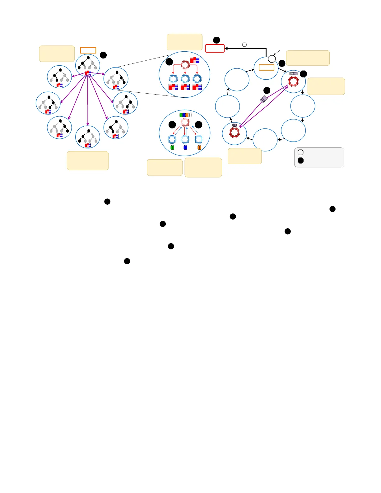
Looking for (Genomic) Needles in a Haystack: Sparsity-Dri v en Search for Identifying Correlated Genetic Mutations in Cancer Ritvik Prabhu ∗ , Emil V atai † ¶ , Bernard Moussad ∗ ¶ , Emmanuel Jeannot § , Ramu Anandakrishnan ‡ , W u-chun Feng ∗ , Mohamed W ahib † ∗ Department of Computer Science , V irginia T ech , Blacksb urg, USA ‡ Biomedical Sciences , Edwar d V ia Colle ge of Osteopathic Medicine , Blacksb urg, USA Email: { ritvikp,bernardm,ramu,wfeng } @vt.edu § Inria, Univ . Bordeaux, LaBRI , T alence, France Email: emmanuel.jeannot@inria.fr † RIKEN Center for Computational Science , K obe, Japan Email: { emil.vatai,mohamed.attia } @rik en.jp Abstract —Cancer typically arises not from a single genetic mutation (i.e., hit) but fr om multi-hit combinations that accumu- late within cells. Howev er , enumerating multi-hit combinations becomes exponentially more expensive computationally as the number of candidate hit gene combinations grow , i.e. C 20 , 000 h , where 20 , 000 is the number of genes in the human genome and h is the number of hits. T o address this challenge, we present an algorithmic framework, called Pruned Depth-First Search (P- DFS) that leverages the high sparsity in tumor mutation data to prune large portions of the search space. Specifically , P-DFS (the main contribution of this paper) - a pruning technique that exploits sparsity to drastically reduce the otherwise exponential h -hit sear ch space for candidate combinations used by W eighted Set Co ver - which is grounded in a depth-first search backtracking technique, prunes infeasible gene subsets early , while a standard greedy weighted set cover (WSC) formulation systematically scores and selects the most discriminative combinations. By intertwining these ideas with optimized bitwise operations and a scalable distributed algorithm on high-performance com- puting clusters, our algorithm can achieve ≈ 90 - 98% reduction in visited combinations for 4-hits, and roughly a 183 × speedup over the exhaustive set cover appr oach (which is algorithmically NP-complete) measured on 147,456 ranks. In doing so, our method can feasibly handle f our -hit and even higher-order gene hits, achie ving both speed and resour ce efficiency . I . I N T RO D U C T I O N Genetic mutations occur routinely in our cells, yet most of these mutations are benign. Occasionally , ho wev er, a specific subset of mutations arises that can pav e the way for cancer dev elopment. Cancer itself is not a single disease, rather, it is a div erse group of disorders defined by unchecked cell growth [1]. Despite decades of effort, it remains the second leading cause of death worldwide, projected to claim around 618,120 li ves in the United States alone in 2025 [2]. The crux of the challenge lies in the fact that cancer typically does not emerge from a single genetic mutation (“hit”) but rather from ¶ Emil V atai and Bernard Moussad contributed equally to this work. precise, multi-hit combinations of a small number (typically between 2–9 hits) of genetic alterations [3]. Understanding these multi-hit patterns has profound impli- cations. First, it illustrates how cancer starts and progresses, providing insight into the biological mechanisms behind tumor formation. Second, identifying the exact sets of mutations responsible for a giv en case of cancer can guide the design of more targeted combination therapies [4], [5]. Ne vertheless, pinpointing these critical mutation sets is akin to searching for needles in a genomic haystack. W ith roughly 20,000 genes in the human genome [6], even two-hit combinations yield on the order of 2 × 10 8 possibilities, while four-hit and five-hit combinations balloon into the range of 10 15 to 10 19 , respec- tiv ely . Exhaustiv ely exploring all such combinations quickly ov erwhelms traditional computational approaches; recent esti- mates suggest that identifying all four-hit combinations would require ov er 500 years on a single CPU [7]. T o tackle this challenge, multi-hit combination analysis has emerged as a prominent strategy . At its core, this approach aims to pinpoint which specific combinations of genetic mu- tations are most relev ant to carcinogenesis, i.e. the process by which normal cells transform into cancer cells. One leading paradigm vie ws the task as a weighted set cov er (WSC) prob- lem, an NP-complete problem, where each candidate mutation set “covers” the tumor samples carrying that set and ideally excludes normal samples [8]. Although WSC can be highly accurate, all possible gene combinations must be exhausti vely enumerated, an endeavor that grows exponentially with each additional “hit. ” Even powerful high-performance computing (HPC) systems struggle to search beyond three-hit or four- hit mutation sets without encountering prohibitiv ely large runtimes or system limitations like I/O bottlenecks, memory constraints, and communication ov erhead [7]. T o cope with the exponential explosion of the search space, researchers have explored heuristics that av oid enumerating For each combination of genes, conduct an intersection operation (bitwise AND) between their rows Tumor Samples Normal Samples Genes Genes Pruning (Our Contribution) Section III • Fig. 5 Compute from reduced candidate set Pruning massively reduces the search space 2 3 3 THIS P APER Number of Combinations computed for the BLCA Cancer Previous Method This Paper 2 hit 2.65 x 10 9 2.65 x 10 9 3 hit 1.30 x 10 12 6.93 x 10 1 1 4 hit 6.43 x 10 15 6.42 x 10 14 1 4 5 PREVIOUS METHOD Search space size: candidate h-hit combinations (G ≈ 20,000) WEIGHTED SET COVER 4 Select combination with highest tumor sample coverage and lowest normal sample coverage Compute from full candidate set 2 Select combination with highest tumor sample coverage and lowest normal sample coverage Fig. 1: Overview of w orkflow . 1 Input: tumor and normal mutation matrices, represented as per -gene bitsets ov er samples. 2 – 3 Previous method (exhaustive enumeration): for every h -hit gene combination, the prior pipeline performs a bitwise AND across the corresponding gene ro ws ( 2 ) and computes o ver the full candidate table ( 3 ), which quickly becomes intractable as h grows. 2 – 3 This paper (prune-then-evaluate): our main contribution is P-DFS, a sparsity-driven pruned depth-first search that massively prunes the h -hit search space ( 2 ) before scoring (see §III and Fig. 5). This produces a substantially smaller candidate table to ev aluate ( 3 ), yielding significant compute-time sa vings by av oiding bitwise-AND intersections for the v ast majority of combinations. 4 and 4 Selection step (common to both): choose the candidate combination with highest tumor cov erage and lo west normal coverage, and pass it into the weighted set cov er procedure 5 . The table at the top summarizes the resulting reduction in combinations explored, which becomes more pronounced as the number of hits h increases. the entire combination space. One such approach, BiGPICC, quickly identifies higher-order hits by le veraging a graph- based method. Ho wev er, BiGPICC omits large swaths of the combination space in the name of speed, which can degrade classification accuracy [9]. In practice, then, the cancer-genomics community faces a trade-off: comprehensi ve methods that handle only a few hits versus heuristic-based approaches that find more hits but risk missing the precise “needles” in the genomic haystack. In this paper , we introduce a nov el HPC-driven framework to push the boundary of multi-hit analyses. W e build upon the rigor of WSC-based methodology but overcome its typical limitations through the utilization of advanced supercomputing resources and optimizations that capitalize on the sparsity in- herent to carcinogenesis data. By doing so, our approach navi- gates the massive search space that was pre viously considered intractable. Specifically , we introduce a new algorithm, pruned depth-first sear ch (P-DFS) for trav ersing the search space of multi-hit combinations—our main contrib ution, which reduces the otherwise exhausti ve candidate search space that dominates WSC-based pipelines (Fig. 1). In particular, we lev erage the high sparsity in gene mutations to do a distributed depth-first search with backtracking to prune the combinatorial search space, thereby shrinking the candidate set before applying the standard greedy WSC selection step, thus dramatically improving the ef ficiency . Through this effort, we seek not only to adv ance our understanding of the genetics underlying cancer but also to provide a practical path toward precisely tailored combination therapies that could improve outcomes for patients worldwide. The remainder of the paper proceeds as follows. In §II, we revie w background and related w ork on multi-hit modeling and search formulations. §III presents our pruned depth-first search (P-DFS) method, including sparsity-aware preprocessing, the core pruning algorithm, and topology-a ware work distribution with hierarchical collectiv es. §IV reports the results on the Fugaku supercomputer, including datasets, pruning ef ficiency , accuracy on held-out data, load balancing with work stealing, and strong scaling. §V provides a summary of our findings. I I . B AC K G R O U N D A N D R E L A T E D W O R K A. Historical F oundations of the Multi-Hit Concept A seminal moment in understanding cancer’ s genetic ba- sis came from Alfred Knudson’ s 1971 “two-hit hypothesis, ” which suggested that certain cancers, specifically retinoblas- toma, emerge only after mutations ha ve occurred in both copies of a tumor suppressor gene [10]. While Knudson focused on a rare pediatric tumor, his ideas gav e rise to a wave of research showing that various solid tumors (e.g., breast, colon, and colorectal cancers) likely require multiple genetic “hits” to shift from normal cellular regulation to malignant growth [11]–[13]. Fig. 2: V isualization of estimated hit numbers for each cancer type from [3]. Derived from the public domain image by M. Haggstrom (2014) [18]. Over the following decades, scientists increasingly recog- nized that no single “magic number” of hits applies uni versally across all tumor types. This led to a deeper statistical and mathematical modeling of carcinogenesis. Early modeling efforts often assumed relati vely simple, uniform mutation rates across genes [14]–[17], but they could not account for the variability in how fast or slo w different genes accumulate alterations. Building upon these limitations, Anandakrishnan et al. introduced a more data-driven model that focuses on the observed distribution of somatic mutations rather than on any single pre-specified rate [3]. They established that many cancers seem to arise from combinations of between 2 and 9 hits, depending on tumor type. As sho wn in Fig. 2, the number of hits required can vary , reinforcing the idea that cancer is not a single entity but rather a multitude of genetic scenarios each leading to a common endpoint of tumor formation. This insight highlights the importance of de veloping comprehensive computational tools capable of sifting through a large and heterogeneous genomic search space. B. Appr oaches for Identifying Multi-Hit Combinations From a computer science perspectiv e, the multi-hit problem can be formulated as follo ws. Giv en a binary mutation matrix X ∈ { 0 , 1 } G × n , where G is the total number of genes under consideration and n is the number of samples (from patients with and without cancer , to which we refer to as tumor samples and normal samples, respectively). Each row corresponds to a gene and each column to a sample, i.e., x g ,s , the element in the g -th row and s -th column of X is set to 1 if the sample s has a mutation in the gene g (and 0 otherwise). W e say a combination γ = { g 1 , . . . , g h } of h genes, “covers” a particular sample s if all genes are mutated in sample s , i.e., X g 1 ,s = X g 2 ,s = · · · = X g h ,s = 1 . The set of samples cov ered by a single combination γ is denoted by: C ( γ ) = { s : ∀ g ∈ γ , x g ,s = 1 } , (1) while the set of samples covered by a set of combinations Γ is the union of the samples covered by the combinations in the set C (Γ) = ∪ γ ∈ Γ C ( γ ) . As large-scale genomic data became widely accessible (spanning tens of thousands of genes in thousands of samples), finding the specific gene sets that constitute these multi-hit combinations became a computationally daunting task. T wo primary solutions have emer ged to address this challenge: (i) methods grounded in the weighted set cover (WSC) problem and (ii) graph-based approaches. 1) W eighted Set Cover (WSC) P aradigm: One of the most prominent solution strategies for multi-hit analysis is to for- mulate the problem as a weighted set cover (WSC) [7], [8], [19]. Here, the aim is to find a set of combinations with minimal weights that cov er all tumor samples. That is, each combination γ has a weight F ( γ ) associated with it, and the goal is to find the set of combinations Γ ∗ that has minimal combined weight among the sets that also covers the tumor samples. Formally , denoting the set of all h gene combinations with Γ h , the minimality objectiv e can be stated as F (Γ ∗ ) = min Γ ⊂ Γ h { F (Γ) } i.e., Γ ∗ = argmin Γ ⊂ Γ h { F (Γ) } (2) while T ⊂ C (Γ ∗ ) expresses the fact that Γ ∗ cov ers the tumor samples, T (where, C (Γ) = ∪ γ ∈ Γ C ( γ ) ). a) Scoring and Algorithmic Steps: As an example of a WSC-based method, Dash et al. [19] maps the multi-hit problem to WSC and applies a greedy strategy to find sets of genes that appear frequently in tumor samples but rar ely in normal samples. Formally , let N t ( X ) and N n ( X ) be the total number of tumor and normal samples, respectiv ely . For each h -hit gene combination γ , T + ( γ , X ) is the number of tumor samples that contain all g ∈ γ genes (true positiv es), and T − ( γ , X ) the number of normal samples that do not contain any of the h genes in the combination (true ne gati ves). A commonly used objectiv e or “weight” function is [19]: F ( γ , X ) = α T + ( γ , X ) + T − ( γ , X ) N t ( X ) + N n ( X ) , where α (often set to 0 . 1 ) penalizes the approach’ s inherent bias toward maximizing T + ov er T − . Until all tumor samples are covered, the algorithm, greedily selects the h -hit combi- nation γ ∗ with the highest F ( γ , X ) value, and remov es the samples (i.e., columns) from X which are covered by γ ∗ as described by Algorithm 1. Algorithm 1 Greedy Set Cover Require: X gene mutation matrix, T indices of tumor sam- ples, h number of hits Ensure: Γ covers T , i.e., T ⊂ C (Γ) 1: C ← ∅ ▷ Set of cov ered samples 2: Γ ← ∅ ▷ The variable holding the results 3: while C ⊊ T do ▷ Are all tumors samples cov ered? 4: γ ∗ ← argmax γ ∈ Γ h F ( γ , X ) ▷ Get the best combination 5: Γ ← Γ ∪ { γ ∗ } ▷ Append γ ∗ to the results 6: C ← C ∪ C ( γ ∗ ) ▷ Update the set of cov ered samples 7: X ← D E L C O L S ( X , γ ∗ ) ▷ Remov e samples from X 8: end while 9: return Γ b) Computational Complexity: While straightforward in concept, enumerating all possible h -gene sets in line 4 of Algorithm 1 is computationally costly . The total number of h -gene combinations is M =  G h  , where G is on the order of 20,000 genes. Even for h = 4 , M ≈ 7 × 10 15 , making an e xhaustiv e search prohibitiv e. Formally , WSC is an NP-complete problem with no known polynomial-time exact solution [7]. Approximate or greedy algorithms reduce the worst-case complexity to O ( M × N t ) , which is still tractable only for small h . Thus, early multi-hit approaches using WSC focused on 2-hit or 3-hit gene sets, and more recent GPU- accelerated methods extended these analyses up to 5 hits [7], [8], [20]. Ho we ver , jumping to 6-hit combinations (much less 8 or 9) remains lar gely infeasible via exhausti ve enumeration or naiv e greedy methods. c) Pruned and P arallel DFS for Candidate Generation: A common way to mitigate the  G h  blowup is to treat Γ h as an implicit search tree and trav erse it with depth-first search (DFS), while pruning subtrees that cannot yield useful candi- dates. This idea is well established in frequent itemset mining: DFS-style enumeration of h -way co-occurrences is paired with anti-monotone bounds to prune away large portions of the candidate lattice [21]–[23]. At scale, these DFS/backtracking trees are routinely parallelized by partitioning the search space (often by prefixes) and using dynamic load balancing like randomized work donation or work stealing, to handle highly irregular subtree sizes [24]–[26]. In the same spirit, our approach uses a pruned, parallel DFS to generate and score only promising h -hit candidates, rather than explicitly materializing all of Γ h . Although exact set-cover solvers can use Branch and Bound (B&B) with relaxation-based bounds for safe pruning, we do not use B&B because our WSC-style greedy routine does not maintain such bounds [27]. 2) Graph-Based Repr esentations: While WSC aims to enu- merate combinations explicitly , graph-based methods, such as BiGPICC [9], represent genomic data in the form of bipartite networks with gene nodes on one side and sample nodes on the other . Edges exist only if a gene is mutated in a gi ven sample. Clustering algorithms (like the Leiden method [28]) then aim to group genes that frequently co-occur across patients. a) Speed vs. Coverage: Graph-based strategies often reduce computational costs compared to full or partial enu- merations. By clustering co-mutated genes, they can ef ficiently highlight general mutation patterns across large datasets. How- ev er, the trade-off is that crucial mutations may be missed when aggregated into clusters, which as a result, affects the classification accuracy as compared to the WSC approach. Thus, graph-based solutions are often preferred for quick large-scale screening or when fewer computational resources are available, but they may miss subtle “needle-in-a-haystack” multi-hit combinations. I I I . P R U N E D D E P T H - F I R S T S E A R C H ( P - D F S ) : P RU N I N G A L G O R I T H M F O R h - H I T G E N E M U T A T I O N S A. Motivation Our goal is to disco ver multi-hit gene combinations efficiently—in a reasonable amount of time—without sacri- ficing accuracy . W e therefore build on the WSC paradigm, which directly optimizes tumor/normal discrimination rather than relying solely on graph clustering, which may blur the sample-lev el signal, and focus our contribution on shrinking the otherwise exhausti ve h -hit candidate search space (via sparsity-driv en pruning) while keeping the WSC scoring ob- jectiv e unchanged. The first empirical observ ation motiv ating our design is the fact that the main loop in Algorithm 1 is executed at most a tens of times. More concretely , in datasets studied by prior work, the greedy cover typically terminated in ≤ 20 iterations [8], [19]. The program spends most of its time ex ecuting the greedy maximum search in step 4, so optimizing this step automatically impro ves the performance of the whole application. Another key observation behind the motiv ation is the extreme sparsity of somatic-mutation matrices. Most entries are zero: each tumor harbors alterations in only a small subset of genes, and each gene is altered in only a small subset of tumors. This “few mountains, many hills” profile and pathway-lev el mutual exclusivity hav e been extensiv ely documented in cancer genomics [29]. Our datasets follo w the same pattern, where the median sparsity is 95.61% (Fig. 3), which immediately suggests algorithmic opportunities. The challenge in the original WSC approach is the combi- natorial gro wth: the number of h -hit candidates scales as  G h  , so even modest increases in h cause an explosion in the search space. T able I shows the number of h -gene candidates,  G h  and the corresponding cancers which require that number of gene hits for diagnosis. Even a one-hit increase yields orders of magnitude more combinations, making naiv e enumeration intractable (calculated here for G =20 , 000 genes). Naiv ely enumerating all combinations to retain WSC’ s accuracy be- comes computationally intractable. Our approach is to exploit sparsity to prune the search space and hence tame the combinatorial explosion while retaining WSC’ s accuracy . Specifically , we structure the computation around early-termination bounds that prune branches as soon as partial intersections go empty . This would le verage the fact that true co-occurrences are rare, so most computation paths Fig. 3: Measured sparsity of all the carcinogenesis mutation matrix datasets av ailable through TCGA. Median: 95.61% . High sparsity underscores the rarity of mutations in all of the cancer datasets. T ABLE I: Combinatorial e xplosion of the WSC search space. Hits Combinations Cancers 2 1 . 99 × 10 08 GBM, O V , UCEC 3 1 . 33 × 10 12 KIRC, LUDA, SKCM, CO AD, BRCA 4 6 . 66 × 10 15 BLCA, HNSC 5 2 . 66 × 10 19 THCA, ST AD, CESC, LUSC 6 8 . 88 × 10 22 LGG 7 2 . 53 × 10 26 DLBC, PRAD, ESCA 8 6 . 34 × 10 29 SARC, KIRP , LIHC 9 1 . 40 × 10 33 UCS, UVM, KICH, MESO, A C, PCPG die quickly , leaving only a small collection of promising sets to ev aluate thoroughly . B. Overview The workflo w of our method consists of several key stages. First, we reorder the binary mutation matrix by gene sparsity , sorting rows from most to least sparse. This sparsity-aware preprocessing enables P-DFS to more effecti vely prune the search space when identifying candidate multi-hit combina- tions. T o ensure efficient parallelization and workload distribu- tion across MPI ranks, we employ a hierarchical work-stealing strategy (as illustrated in Fig. 4). C. Pr epr ocessing W e represent each cohort as a binary mutation matrix with genes as rows and samples as columns (tumor and normal samples are tracked distinctly; see Fig. 5 for an ov ervie w of the workflow). T o accelerate P-DFS, we order gene rows from most sparse to least sparse prior to computation. This sparsity-aware ordering helps the search prune aggressiv ely: combinations b uilt from genes that sho w high sparsity in their mutations can get pruned early , thereby reducing the size of the explored sub-tree. In practice, this simple reordering decreases the number of combination intersections we must ev aluate before a branch is pruned. T o make set operations fast, we represent each gene’ s samples as a bit-vector and implement primitiv e operations like intersection, union, and membership count via bitwise op- erations. This design helps by slashing the memory footprint, hence improving cache residenc y of hot ro ws. D. Cor e Algorithm As discussed in §II-B1b, the bottleneck of the algorithm is trav ersing all the h -hit gene combinations. Instead of scanning the entire search space, we restructure the trav ersal where for each λ , we perform a depth-first expansion with backtracking that prunes as soon as a partial intersection becomes empty . T o ef fectiv ely enable this solution, as mentioned in §III-C, we sort the gene ro ws by incr easing sparsity (i.e., from most zero entries to fewer) to trigger empty partial intersections earlier . For a growing partial set g 1 , . . . , g ℓ we maintain the running intersection y ℓ ← x g 1 ∧ · · · ∧ x g ℓ ov er the tumor cohort (bitwise AND ). If at any step y ℓ = 0 (no tumor sample has all ℓ mutations), we immediately backtrack. There is nothing left to gain by adding more genes on that path, so the entire subtree can be skipped without ev aluation. When we reach depth h with y h  = 0 , we score γ via the objecti ve F ( γ , X ) and update the current best ( F ∗ , γ ∗ ) . This simple rule is powerful in sparse data: many branches become empty after just a few AND s, so we examine far fewer than  G h  combinations. The P-DFS approach does not change the worst-case time complexity of the original WSC search. In other words, if no branch ever empties, it degenerates to full enumeration of  G h  combinations. The algorithm simply aggressi vely prunes the search space in typical sparse cohorts, so the ef fective number of candidates ev aluated (and the wall time) drops substantially . The control flo w is made e xplicit in Algorithm 2: the inner grow-and-check loop maintains the running intersection, and the early-exit test at line 7 performs the pruning. E. W ork Distribution: Scaling and Load Balancing Our search space grows combinatorially with the number of genes and the hit depth, so we must expose massi ve concurrency . A naiv e partition by the first gene yields about 20,000 tasks for 20,000 genes and caps useful parallelism near 20,000 compute units. Instead, we flatten the nested loops ov er g 1 and g 2 into a single λ index so each ( g 1 , g 2 ) pair is an independent task (Fig. 5, 2 ), producing C G 2 ≈  20 , 000 2  tasks—enough ev en at the exascale. Furthermore, pruning makes trav ersal cost per task highly irr egular : some subtrees collapse after only a few intersections while others surviv e and expand. Equal counts of λ s therefore do not imply equal work, and a static partition risks idle ranks and stragglers. This motiv ates the MPI-based, dynamically assigned work distribution described below (see the control-flow overvie w in Fig. 4). a) MPI Execution Model and Data Residency: W e scale with MPI, running one rank per physical core, and assign dis- joint λ sub-intervals to each rank for independent computation. Giv en that the da taset is just a few megabytes in size, each rank holds the entire input table. Furthermore, each rank obtains a subinterval of λ s from [1 , . . . , C G 2 ] . By decoding λ back to ( g 1 , g 2 ) , the state of the program corresponds to step 7 in x 2 in a row steal request T erminate 6 7 1 5 2 req req req 3 4 Rank 0 reads data and broadcasts to all node leaders Rank 0 Each leader broadcasts data within its node Leader assigns fixed-size chunks to workers On completion, worker sends req to leader to obtain the next chunk. T oken starts white and circulates among node leaders. Victim donates half its work and flips token to black. Each node processes a distinct portion of the compute space Idle node sends steal request to a busy node Token Rank 0 Returns No work observed Work observed since last pass Fig. 4: W ork Distrib ution Over view : W e use one MPI rank per core and two communicators: a global communicator among node leaders and a local communicator within each node. The local Rank 0 of each node is the node leader and also belongs to the global communicator . 1 Because the database is only a few MB, Rank 0 reads it from disk and broadcasts the entire database to all node leaders. Each node then computes a distinct subset of λ values, i.e., parallelism is in compute. 2 Each node leader broadcasts the data within its node via the local communicator . 3 The leader tracks outstanding λ values and hands out fixed-sized work chunks to the workers. 4 When a worker finishes its portion of the compute, it sends a short req to the leader . If work remains, the leader issues another chunk, otherwise the worker becomes idle. 5 If a leader exhausts its local queue, it randomly selects a peer to steal from. A busy victim donates roughly half of its remaining range to the thief, while an idle peer triggers a retry with another node. 6 T ermination is decided with a circulating token that starts at Rank 0 in the white state (no work observed) and moves around leaders in ring order . Any node that performs work or donates flips the token to black (work observed). 7 If the token returns to Rank 0 as black, it is reset to white and circulated again. If it returns white twice in a row , all the work to be computed on has been distrib uted, and a termination signal is sent. Algorithm 2, and it can proceed to the first level of pruning if no samples share the mutations of both genes. b) Baseline: centralized master–worker: W e begin with a master–worker design in which rank 0 is the master and all other ranks are workers. The master maintains a single global pool of λ indices and dispenses fixed-size chunks with indices ⟨ start , end ⟩ on demand. Each worker stores only the bounds of its current chunk, computes directly over its priv ate copy of the table, and, upon completion, sends a short request to the master for the next chunk. Using a fixed chunk size keeps assignment constant-time and minimizes bookkeeping, so control traffic remains light. In other words, workers communicate only when pulling new work and when receiving the final termination signal from the master . c) Limitations of centr alized master-worker: A single global master would saturate on large machines. Every request would target one rank, queues would grow , and the MPI progress engine would spend time on control traffic rather than computation. Prior studies of dynamic scheduling report that single point task coordination limits scalability and motiv ates multi-lev el coordinators [30], [31]. W e therefore move to a hierarchical organization that respects the machine topology . d) T opology-awar e hierar chical or ganization: All ranks on a node form a local communicator and designate rank 0 as the node leader . All node leaders form a second communicator that spans nodes. Leaders manage work inside the node, and coordinate only coarse actions across nodes, which reduces cross-node traffic and removes the single choke point. e) T wo-level work stealing: W ork stealing operates at two levels. Inside a node, workers never steal from each other . They always ask the node leader for the next interv al. Across nodes, leaders both request and donate work. When a leader runs out of local work it selects a peer leader and issues a steal request. Peer selection is randomized with a small number of retries in case the chosen leader has no more work to giv e. This spreads requests across the ring of leaders and av oids hot spots. When a leader recei ves a steal request it answers from its own remaining interval. The leader replies with the upper half of its remaining λ -interval. This splits its workload roughly in two, hands a single contiguous block, which is essentially a ⟨ start , end ⟩ interval, to the thief. The victim also records that a donation occurred via a local flag, which is used later during coordination. Input Sor t by row sparsity 1 3 . . . 𝐺 𝑡 1 . . . 𝑛 1 . . . 𝜆 1 ↦→ 𝑥 1 ∧ 𝑥 2 𝜆 2 ↦→ 𝑥 1 ∧ 𝑥 3 . . . 𝜆 𝑖 ↦→ 𝑥 2 ∧ 𝑥 3 𝜆 𝑖 + 1 ↦→ 𝑥 2 ∧ 𝑥 4 . . .  !  !  !  !  ! · · · ∧ 𝑥 3 · · · ∧ 𝑥 4 · · · ∧ 𝑥 5 . . . · · · ∧ 𝑥 𝐺   · · · ∧ 𝑥 4 · · · ∧ 𝑥 5 · · · ∧ 𝑥 6 . . . · · · ∧ 𝑥 𝐺  !  · · · ∧ 𝑥 4 . . .  · · · ∧ 𝑥 5 . . .  · · · ∧ 𝑥 5 . . . · · · ∧ 𝑥 6 · · · ∧ 𝑥 7 . . . · · · ∧ 𝑥 𝐺 𝛾 ∗ Depth 2 Firs t tw o nested loops ( 𝑔 1 and 𝑔 2 ) are flattened into a single 𝜆 loop Depth 3 Third nested loop ( 𝑔 3 ) Depth 4 Fourth nested loop ( 𝑔 4 ) A dd 𝛾 ∗ to the solution/co v er set 𝐹 ( 𝛾 ∗ , 𝑋 ) = max 𝛾 𝐹 ( 𝛾 , 𝑋 )  DelC ols ( 𝑋 , 𝛾 ∗ )  Prune ! Keep P -DFS Greedy W SC 1 2 3 4 5 6 7 8 Fig. 5: Pruned depth-first search (P-DFS): pruning algorithm for h -hit gene mutations (with h = 4 ): In the preprocessing step, the input data is sorted 1 based on row sparsity to improve pruning efficienc y . The first two of the four nested loops, with iterators g 1 and g 2 are flattened into a single λ -loop 2 to enable work distribution with a high number of workers. In each iteration of the λ -loop the partial combination using only rows g 1 and g 2 are computed. If all the tumor samples are zero/false, the combination cannot contrib ute to the set cov er (empty cov er), nor would the resulting, higher hit combinations, so the entire subtree can be skipped 3 . Otherwise, the algorithm proceeds to the depth 3 nested loop 4 of the search tree, computing the 3-hit combination (using the 2-hit partial results) and similar eliminates empty cov ers 5 or proceeds to depth 4 as needed 6 . The γ ∗ combination with the best F ( γ , X ) value is saved 7 and the samples (columns) covered by it are remov ed 8 from the input database for the next iteration. f) Barrier-fr ee termination detection: T ermination and global progress use a token on the leader communicator . Leaders form a logical ring. The root creates a white token and sends it to the next leader . A leader forwards the token only when it is idle and has no local work, and if it has donated work since it last saw the token it turns the token black before forwarding. If the root receives a white token twice in succession while it is idle, there is no outstanding work. The root then sets the termination flag via MPI one- sided communication, issuing an MPI_Put into a shared RMA window , and each leader notifies its work ers to exit their request loop. This protocol detects quiescence without a global barrier and remains robust under random steals, since the black color records backward donations and suppresses premature termination. g) Hierar chical collectives: Broadcast and AllReduce: Reductions and broadcasts follow an identical hierarchy struc- ture. First, within each node, processes reduce onto a des- ignated leader using intranode collectiv es that exploit shared memory . The leaders then perform the internode collectiv e on the leader communicator . Finally , each leader distributes the result back to its local workers via an intranode broadcast. Although this hierarchical framework increases memory con- sumption, it reduces message traffic on the network fabric and shortens the critical path for large collecti ves, which is crucial on systems where MPI buf fers and progress threads face significant contention at scale (realistic benchmarks demon- strate up to a 7× speedup for all-reduce using these two-lev el structures compared to standard MPI Allreduce). h) Communication pr ofile and the MPI-only choice: Giv en that we replicate the gene–sample mutation table per rank, all the inner loop work memory stays local to the node and communication is confined to work requests, inter- leader steals, hierarchical collectives, and a final termination flag. W e prefer rank-per-core ov er hybrid MPI+OpenMP for this irregular , fine-grained workload because thread schedulers introduce overheads from frequent returns to the scheduler, extra barriers, and affinity or NUMA pitfalls, which can make hybrid slower than pure MPI without careful tuning [32], [33]. F . Pre-sorted DFS F inds Smaller Covers at Higher Hit Thr esholds An advantage of our algorithm is that it yields better solutions, i.e., smaller set cov ers, at higher hit thresholds. Algorithm 2 P-DFS : Implementing step 4 of Algorithm 1 as a depth-first maximum search with backtracking. Require: X gene mutation matrix, h number of hits Ensure: γ ∗ = argmax γ ∈ Γ h F ( γ , X ) 1: F ∗ ← −∞ ▷ Initialize maximum search 2: for g 1 = 1 to G − h + 1 do ▷ Depth 1 3: γ ← g 1 ▷ The g 1 -th row of X 4: for g 2 = g 1 + 1 to G − h + 2 do ▷ Depth 2 5: γ ← γ ∪ g 2 ▷ Implemented as element-wise logical AND 6: if x g 1 ∧ x g 2 = 0 then 7: continue ▷ Eliminate brach 8: end if 9: . . . 10: for g h = g h − 1 + 1 to G do ▷ Depth h 11: γ ← γ ∪ { g h } 12: F ← F ( γ , X ) 13: if F > F ∗ then ▷ Maximum search 14: F ∗ ← F ; γ ∗ ← γ 15: end if 16: end for 17: . . . 18: end for 19: end for 20: return γ ∗ T ABLE II: Comparison of Proposed Algorithm vs. Original WSC Solution Size for V arious Cancers and Hit Sizes Cancer Hit Size Pr oposed Algorithm Original WSC BLCA 2 17 15 GBM 2 11 N/A O V 2 9 N/A UCEC 2 5 9 BLCA 3 16 12 BRCA 3 12 8 CO AD 3 12 10 KIRC 3 9 6 LU AD 3 13 10 SKCM 3 11 N/A BLCA 4 16 19 HNSC 4 13 17 As sho wn in T able II, with our algorithm we reduce the solution size at four hits by 80% average. Since the size of the solution space grows exponentially with the number of hits, obtaining smaller cov er sets at higher number of hits provides a substantial performance benefit, as the search can terminate earlier once a minimal cover is found. In this section, we analyze why the proposed algorithm tends to produce smaller cov er sets at higher hit thresholds. As introduced in Eq. (2), our goal is to find the set of combinations that has a minimal combined weight. While the baseline explores combinations randomly , the proposed algorithm sorts genes, i.e. matrix rows, by sparsity (from fe wer to more mutations), and uses P-DFS to prune the search space of combinations. 1) Effect of sparsity at high h : When the number of hits h is small (e.g., h = 2 ), dense genes with many mutations quickly increase the hit coverage C defined in Eq. (1) even if they ov erlap strongly . At higher h , howe ver , overlapping dense genes provide less new information, because many samples already share the same mutations. Thus, the expected marginal gain of a gene g gi ven the current partially constructed combination of genes γ , ∆ h ( g | γ ) = C ( γ ∪ { g } ) − C ( γ ) , decreases more sharply for dense genes as h increases. Sparse genes, which cover fewer b ut more distinct samples, maintain higher marginal gain when h is large. 2) Pruning advantage: Because our search visits sparse genes first, partial solutions grow coverage efficiently with minimal redundancy . This makes the upper bound on remain- ing possible gain, U h ( γ ) = max S ⊆ Γ h \ γ C ( γ ∪ S ) − C ( γ ) , drop faster as the search deepens. Branches that cannot reach the target are pruned earlier . At higher h , the redundancy among dense genes strengthens this effect, reducing the ef fecti ve branching factor and shrinking the explored tree from O (2 n ) tow ard O (2 L ) , where L is the number of sparse, high-value genes. 3) Resulting behavior: This explains why the proposed method produces smaller cov ers at h = 4 . For large h , sparse-first ordering better matches the structure of the residual samples, yields higher marginal gains per added gene, and enables tighter pruning. In contrast, random or dense-first exploration revisits many redundant re gions, leading to larger cov ers or slower con vergence. Empirically , this aligns with our results, where P-DFS achieves smaller solution sizes at 4-hit thresholds. I V . R E S U L T S A N D D I S C U S S I O N A. Experimental Platform: Fugaku All experiments were conducted on the supercomputer Fugaku, located in K obe, Japan. Each node contains a single Fujitsu A64FX processor with 48 compute cores and 32 GB of HBM2 memory . W e use Fujitsu MPI and run one MPI rank per core with no intra-rank threading. This choice avoids thread- scheduler ov erheads and lets each rank maintain a priv ate copy of the data. Our datasets are only a few megabytes per cohort, so replication across 48 ranks comfortably fits within the 32 GB node memory budget and removes contention on shared data structures. Nodes are connected by the T ofu-D interconnect in a six- dimensional mesh–torus topology . W e request compact alloca- tions that form near-cubic sub-tori so that the job spans similar extents in each of the six dimensions. This placement reduces av erage hop distance, preserves bisection bandwidth, and helps keep collectiv e and point-to-point costs stable as we scale out. The node counts in our strong-scaling studies { 192, 384, 768, 1,536, 3,072 } were chosen because they tile the 6D topology cleanly and allow the scheduler to pack jobs contiguously . Our MPI configuration follows the algorithmic design. A single leader rank per job performs interval assignment, and all other ranks act as workers that compute against their priv ate tables. W e bind one rank to one physical core and pin memory locally to improve cache residency on A64FX. Communication consists of short messages to pull work and a few global notifications at the end of the run. On T ofu-D these messages trav erse fe w hops under compact placement, which keeps the communication term nearly constant across scales, as observ ed in §IV -F. The combination of rank-per-core, data replication, and compact topology-aware placement is what allows the pruned workload to remain compute dominated o ver a wide range of node counts. B. Dataset Somatic mutation data in the Mutation Annotation For - mat (MAF) was acquired from The Cancer Genome Atlas (TCGA) [34]. All mutations were identified via the Mutect2 software, a commonly utilized tool in the genomic community . Each cancer type was processed individually , extracting gene- lev el mutations paired with patient sample identifiers. Silent mutations were excluded to focus on potentially functional variants. Follo wing preprocessing, each dataset was divided into train and test sets at 75% and 25%, respectiv ely . C. Pruning Efficiency and End-to-End Runtime A central outcome of our approach is that we only visit a tiny fraction of the potential h -hit combinations. For each cohort, we tracked the exact number of combinations that the P-DFS tra versal ev aluated and compared it to a non- pruning baseline whose search space equals the combinatorial maximum  20 , 000 h  . Cohorts are paired with the hit sizes reported in [3], which estimates the number of hits for 17 cancer types with at least 200 samples. Fig. 6 reports, for multiple cohorts and hit sizes, the normal- ized number of combinations that are actually visited by our algorithm. The blue bars represent the total search space and are normalized to 1 . 0 by construction. The orange bars show the fraction we visit. Lower orange bars indicate more pruning. W e observe a consistent drop in visitation as h increases. This behavior is expected because early intersections become empty much more often at higher h . In sparse mutation matrices, the probability that a sample carries all genes in a growing partial set decreases rapidly with each added gene. The result is aggressiv e pruning at higher hit sizes and a dramatic reduction in ev aluated candidates. Pruning translates directly into wall-time gains. W e study this effect with a 4-hit run for BLCA across 192, 384, 768, 1,536, and 3,072 nodes. W e also plot an ideal strong-scaling line for the pruned workload to check whether runtime falls in in verse proportion to node count. For a fixed workload of size M N t the ideal time on N nodes is T ideal ( N ) = c M N t N , where M is the number of combinations actually visited by the algorithm, N t is the number of tumor samples, and c is a platform constant that captures per-combination cost. W e Fig. 6: Pruned search vs. theoretical maximum. For each cohort and hit size, the total combinations  20 , 000 h  are nor- malized to 1 . 0 (blue). The orange bars show the fraction of combinations actually visited by our sparsity-driven P-DFS method. calibrate c from the 192-node run, c = T measured (192) · 192 M N t , which yields T ideal ( N ) = T measured (192) · 192 N . The bounded curve lies close to this line up to 768 nodes but shows slight di ver gence beyond 768 nodes. T o highlight the value of pruning, we also ex ecuted a baseline run at 3,072 nodes. This job did not finish within the four-hour allocation. Based on the completed portion, we estimate a time to solution of about 52 hours on 3,072 nodes. This projected time is much slower than the P-DFS method ev en at 192 nodes. The gap reflects the massiv e volume of candidates that fail the first few intersection checks and yet must still be ev aluated when pruning is disabled. T aken together, Figs. 6 and 7 show that our design de- liv ers much better performance compared to the brute-force weighted set cover algorithm. The algorithm prunes vast regions of the search space before computing the weights. D. Accuracy on Held-out Data W e e v aluate accurac y of the P-DFS method with a random 75% – 25% train–test split per cohort. On the training set, the algorithm learns a small set of h -hit gene combinations using P-DFS weighted set cover method. W e then freeze those combinations and assess coverage on the disjoint T est set. For each cohort we report: • T umor Covered : number of tumor samples that contain at least one learned h -hit combination. • Normal Cov ered : number of normal samples that contain at least one learned h -hit combination. Fig. 7: W all time vs. scale for 4 hits . Measured wall times for the P-DFS runs across nodes, together with the ideal strong- scaling line. T ABLE III: Training split ( 75% ). T umor and normal coverage and deriv ed sensitivity/specificity for learned combinations. Cancer Hits TC TT NC NT Sens. Spec. BLCA 4 309 309 0 248 1.0 1.0 HNSC 4 382 382 0 248 1.0 1.0 BLCA 3 309 309 0 248 1.0 1.0 BRCA 3 786 786 8 248 1.0 0.9677 CO AD 3 325 325 4 248 1.0 0.9839 KIRC 3 288 288 1 248 1.0 0.9960 LU AD 3 426 426 0 248 1.0 1.0 SKCM 3 352 352 0 248 1.0 1.0 GBM 2 297 297 0 248 1.0 1.0 O V 2 319 319 2 248 1.0 0.9919 UCEC 2 406 406 8 248 1.0 0.9677 BLCA 2 309 309 0 248 1.0 1.0 a) T raining performance: T able III summarizes results on the training split (TC, TT , NC, NT , Sens. and Spec. correspond to number of cov ered tumor samples, total number of tumor samples, number of covered normal samples, total number of normal samples, sensiti vity and specificity , respec- tiv ely). Sensiti vity is 1 . 0 for all cohorts, and specificity is very high, with small leakage into normals for BRCA, COAD, KIRC, O V , and UCEC. These results are expected because the model is optimized on the training set. Furthermore, these values represent an upper bound on achiev able performance for a giv en h . b) Generalization: T able IV reports performance on the disjoint 25% test split using the combinations learned on train- ing (column names detailed in §IV -D0a). Sensitivity remains high across cohorts ( 0 . 85 – 0 . 98 ), and specificity is similarly strong ( 0 . 81 – 0 . 99 ). The small reduction relativ e to training reflects that some held-out tumors lack the exact h -hit patterns selected during training. c) T akeaways: Across ten cohorts and hit sizes guided by [3], our approach achieves near-perfect sensitivity and very high specificity on training, and maintains strong accuracy on T ABLE IV: Held-out T est split ( 25% ). Coverage-based sen- sitivity and specificity using combinations learned on the T raining split. Cancer Hits TC TT NC NT Sens. Spec. BLCA 4 88 103 16 83 0.8544 0.8072 HNSC 4 113 128 14 83 0.8828 0.8313 BLCA 3 89 103 12 83 0.8641 0.8554 BRCA 3 257 262 13 83 0.9809 0.8434 CO AD 3 97 109 8 83 0.8899 0.9036 KIRC 3 92 97 8 83 0.9485 0.9036 LU AD 3 124 143 14 83 0.8671 0.8313 SKCM 3 106 118 7 83 0.8983 0.9157 BLCA 2 88 103 6 83 0.8544 0.9277 GBM 2 95 99 1 83 0.9596 0.9880 O V 2 102 107 3 83 0.9533 0.9639 UCEC 2 131 136 5 83 0.9632 0.9398 test data. High test sensitivity indicates that the selected h - hit patterns capture tumor signal that generalizes to unseen patients. High test specificity sho ws that normal tissue rarely matches these patterns. Combined with the pruning and scaling results, these accuracy outcomes demonstrate that the algo- rithm is biologically discriminativ e at scale. E. Load Balancing and the Impact of W ork Stealing W e quantify the effect of irregularity by measuring the worker running time on BLCA with 4 hits at 1,536 nodes. W orker running time records only periods when a worker is computing, not idle or waiting on the leader . W e run the same configuration with work stealing enabled and disabled and collect per-w orker histograms. Fig. 8 shows the distributions. W ithout stealing the distrib u- tion is broad with heavy right tails, which indicates that many workers receiv e subtrees that are much larger than average. W ith stealing the distrib ution collapses into a sharp peak. The standard deviation drops from 544 . 186 seconds without stealing to 41 . 9599 seconds with stealing, a 13 × reduction in spread. Likewise, we observed average worker idleness likewise falls from 63 . 61% (no stealing) to 22 . 31% (with stealing), reinf orcing the benefits of work stealing. This indicates that workers finish at nearly the same time when stealing is enabled. The reduced spread and a verage idleness of the workers aligns with the lower wall times reported in Fig. 7, since long stragglers can dominate end-to-end time. F . Strong Scaling Acr oss Hit Sizes W e now quantify the parallel ef ficiency across hit sizes using speedup from a 192-node baseline. For each cohort we keep the algorithm and implementation fixed: P-DFS method with work stealing, and only vary the node count N ∈ { 192 , 384 , 768 , 1536 , 3072 } . A key trend stands out: scaling improves as the hit count increases, with BLCA (4 hits) tracking the ideal most closely , BRCA (3 hits) in the middle, and O V (2 hits) saturating early . Before interpreting Fig. 8: Per -worker running-time distributions for BLCA, 4 hits, 1,536 nodes. Fig. 9: W all-time breakdown of BLCA at 4 hits. the speedup curves, we first examine what fraction of wall time is computation versus communication. Fig. 9 decomposes wall time into worker running time and communication for BLCA at 4 hits. Communication is comparativ ely constant across scales, while worker running time f alls with node count as expected for a compute- dominated phase. When the compute term is large the constant is amortized and strong scaling holds. When the compute term is small the communication limits the additional speedup. W ith this context we return to the speedup curves. After pruning, the useful work is proportional to M N t , where M is the number of combinations actually visited and N t is the number of tumor samples. A simple model T ( N ) ≈ c M N t N + T comm explains the observ ations. For low hit counts, M is small because intersections go empty early , so c M N t N becomes comparable to the constant T comm at modest N . The O V (2-hit) curve therefore plateaus and even dips as noise and fixed ov erheads dominate. As the hit count increases, more combinations surviv e pruning, so M is larger and the compute term dominates over a wider range of N . BRCA (3 hits) impro ves over O V , and BLCA (4 hits) stays close to the ideal line because the run remains compute bound ev en at 3,072 nodes. Fig. 10: Strong scaling speedup from 192 to 3,072 nodes for BLCA 4-hit, BRCA 3-hit, and O V 2-hit datasets. V . C O N C L U S I O N W e present a sparsity-aware depth-first search algorithm with backtracking that serv es as our main contrib ution: a pruning technique for the weighted set cover (WSC) pipeline, called pruned depth-first sear ch , for discovering multi-hit gene combinations. By sorting genes by sparsity , maintaining running bitset intersections, and backtracking as soon as partial cov ers are found to be empty , the search algorithm discards vast swaths of the combinatorial space (i.e., reduces the candidate search space) before scoring with the (standard) WSC selection step. T o expose parallelism, we flatten the first two nested loops of the WSC algorithm into a single λ index and distribute contiguous ⟨ start , end ⟩ intervals, enabling high worker counts. A hierarchical MPI design, with per-node leader , lightweight request/response assignment, and barrier- free termination, keeps control traffic low and av oids single- master bottlenecks. Empirically , pruning grows more effecti vely with the hit threshold. In other words, higher h induces emptier partial intersections, shrinking the visited space and reducing wall time relative to exhaustiv e WSC enumeration. On Fugaku, we observe that strong scaling improved as we increase the number of hits being computed. Furthermore, we observe tighter load-balance distributions when hierarchical scheduling is enabled. Across cohorts, the resulting combinations achie ve high sensitivity and specificity on held-out data (via ran- dom 75% – 25% splits), indicating that sparsity-driven pruning, paired with weighted set-cover scoring yields patterns that generalize. T aken together , these results demonstrate that P- DFS pruning con verts an otherwise intractable enumeration into a high-throughput search at scale. C O D E A V A I L A B I L I T Y The reference implementation and scripts to reproduce our results are av ailable at https://github .com/RitvikPrabhu/ P- DFS- Multihit- WSC. A C K N O W L E D G M E N T S W e thank Niteya Shah for constructi ve comments and feedback on an early draft of this paper . R E F E R E N C E S [1] J. S. Brown, S. R. Amend, R. H. Austin, R. A. Gatenby , E. U. Hammarlund, and K. J. Pienta, “Updating the Definition of Cancer, ” Molecular Cancer Resear ch , vol. 21, no. 11, pp. 1142–1147, Nov . 2023. [Online]. A vailable: https://doi.org/10.1158/1541- 7786.MCR- 23- 0411 [2] R. L. Sie gel, T . B. Kratzer , A. N. Giaquinto, H. Sung, and A. Jemal, “Cancer Statistics, 2025, ” CA: A Cancer Journal for Clinicians , vol. 75, no. 1, pp. 10–45, 2025, eprint: https://onlinelibrary .wiley .com/doi/pdf/10.3322/caac.21871. [Online]. A vailable: https://onlinelibrary .wiley .com/doi/abs/10.3322/caac.21871 [3] R. Anandakrishnan, R. T . V arghese, N. A. Kinne y , and H. R. Garner , “Estimating the Number of Genetic Mutations (hits) Required for Carcinogenesis Based on the Distribution of Somatic Mutations, ” PLoS Computational Biology , v ol. 15, no. 3, p. e1006881, Mar . 2019. [Online]. A vailable: https://www .ncbi.nlm.nih.gov/pmc/articles/PMC6424461/ [4] B. Al-Lazikani, U. Banerji, and P . W orkman, “Combinatorial Drug Therapy for Cancer in the Post-Genomic Era, ” Natur e Biotechnology , vol. 30, no. 7, pp. 679–692, Jul. 2012. [5] H. Ledford, “Cocktails for Cancer with a Measure of Immunotherapy, ” Natur e , v ol. 532, no. 7598, pp. 162–164, Apr. 2016, publisher: Nature Publishing Group. [Online]. A vailable: https://www .nature.com/articles/ 532162a [6] International Human Genome Sequencing Consortium, “Finishing the Euchromatic Sequence of the Human Genome, ” Natur e , vol. 431, no. 7011, pp. 931–945, Oct. 2004, publisher: Nature Publishing Group. [Online]. A vailable: https://www .nature.com/articles/nature03001 [7] S. Dash, Q. Al-Hajri, W .-c. Feng, H. R. Garner, and R. Anandakrishnan, “Scaling Out a Combinatorial Algorithm for Discov ering Carcinogenic Gene Combinations to Thousands of GPUs, ” in 2021 IEEE International P arallel and Distributed Processing Symposium (IPDPS) . Portland, OR, USA: IEEE, May 2021, pp. 837–846. [Online]. A vailable: https://ieeexplore.ieee.or g/document/9460537/ [8] Q. Al Hajri, S. Dash, W .-c. Feng, H. R. Garner , and R. Anandakrishnan, “Identifying Multi-Hit Carcinogenic Gene Combinations: Scaling up a W eighted Set Cover Algorithm Using Compressed Binary Matrix Representation on a GPU, ” Scientific Reports , vol. 10, no. 1, p. 2022, Feb . 2020, publisher: Nature Publishing Group. [Online]. A vailable: https://www .nature.com/articles/s41598- 020- 58785- y [9] V . Oles, S. Dash, and R. Anandakrishnan, “BiGPICC: A Graph- Based Approach to Identifying Carcinogenic Gene Combinations from Mutation Data, ” Feb. 2023, pages: 2023.02.06.527327 Section: New Results. [Online]. A vailable: https://www .biorxi v .org/content/10.1101/ 2023.02.06.527327v1 [10] A. G. Knudson, “Mutation and Cancer: Statistical Study of Retinoblas- toma, ” Proceedings of the National Academy of Sciences of the United States of America , vol. 68, no. 4, pp. 820–823, Apr . 1971. [Online]. A vailable: https://www .ncbi.nlm.nih.gov/pmc/articles/PMC389051/ [11] X. Zhang and R. Simon, “Estimating the Number of Rate Limiting Genomic Changes for Human Breast Cancer, ” Breast Cancer Research and T r eatment , vol. 91, no. 2, pp. 121–124, May 2005. [Online]. A vailable: https://doi.org/10.1007/s10549- 004- 5782- y [12] C. T omasetti, L. Marchionni, M. A. Nowak, G. Parmigiani, and B. V ogelstein, “Only Three Driver Gene Mutations are Required for the Dev elopment of Lung and Colorectal Cancers, ” Pr oceedings of the National Academy of Sciences of the United States of America , vol. 112, no. 1, pp. 118–123, Jan. 2015. [Online]. A vailable: https://www .ncbi.nlm.nih.gov/pmc/articles/PMC4291633/ [13] M. P . Little and E. G. Wright, “A Stochastic Carcinogenesis Model Incorporating Genomic Instability Fitted to Colon Cancer Data, ” Mathematical Biosciences , vol. 183, no. 2, pp. 111–134, Jun. 2003. [Online]. A vailable: https://www .sciencedirect.com/science/article/pii/ S0025556403000403 [14] J. H. Bavarv a, H. T ae, L. McIver, E. Karunasena, and H. R. Garner , “The Dynamic Exome: acquired variants as individuals age, ” Aging (Albany NY) , vol. 6, no. 6, pp. 511–521, Jun. 2014. [Online]. A vailable: https://www .ncbi.nlm.nih.gov/pmc/articles/PMC4100812/ [15] X. Wu, E. D. Strome, Q. Meng, P . J. Hastings, S. E. Plon, and M. Kimmel, “A Robust Estimator of Mutation Rates, ” Mutation Resear ch/Fundamental and Molecular Mechanisms of Mutagenesis , vol. 661, no. 1, pp. 101–109, Feb. 2009. [Online]. A vailable: https://www .sciencedirect.com/science/article/pii/S0027510708003084 [16] L. B. Alexandrov , P . H. Jones, D. C. W edge, J. E. Sale, P . J. Campbell, S. Nik-Zainal, and M. R. Stratton, “Clock-like Mutational Processes in Human Somatic Cells, ” Nature genetics , vol. 47, no. 12, pp. 1402–1407, Dec. 2015. [Online]. A vailable: https://www .ncbi.nlm.nih.gov/pmc/articles/PMC4783858/ [17] Y . R. Paashuis-Lew and J. A. Heddle, “Spontaneous Mutation During Fetal Development and Post-Natal Growth, ” Mutagenesis , vol. 13, no. 6, pp. 613–617, Nov . 1998. [18] Wiki versity , “W ikiJournal of Medicine/Medical Gallery of Mikael H ¨ aggstr ¨ om 2014 — W ikiv ersity ,, ” 2024, [Online; accessed 25-September-2024]. [Online]. A vailable: https://en.wikiv ersity .org/w/ index.php?title=W ikiJournal of Medicine/Medical gallery of Mikael H%C3%A4ggstr%C3%B6m 2014&oldid=2655064 [19] S. Dash, N. A. Kinney , R. T . V arghese, H. R. Garner , W .-c. Feng, and R. Anandakrishnan, “Differentiating Between Cancer and Normal T issue Samples Using Multi-Hit Combinations of Genetic Mutations, ” Scientific Reports , vol. 9, no. 1, p. 1005, Jan. 2019. [Online]. A vailable: https://www .nature.com/articles/s41598- 018- 37835- 6 [20] S. Dash, M. A. Haque Monil, J. Yin, R. Anandakrishnan, and F . W ang, “Distributing Simplex-Shaped Nested for-Loops to Identify Carcinogenic Gene Combinations, ” in 2023 IEEE International P arallel and Distributed Pr ocessing Symposium (IPDPS) , May 2023, pp. 974–984, iSSN: 1530-2075. [Online]. A v ailable: https: //ieeexplore.ieee.or g/abstract/document/10177404 [21] C. Borgelt, “Frequent Item Set Mining, ” W iley Inter disciplinary Reviews: Data Mining and Knowledge Discovery , vol. 2, no. 6, pp. 437–456, 2012. [22] T . Uno, T . Asai, Y . Uchida, and H. Arimura, “LCM: An Efficient Algorithm for Enumerating Frequent Closed Item Sets.” in Fimi , v ol. 90, 2003. [23] J. M. Luna, P . Fournier-V iger, and S. V entura, “Frequent Itemset Mining: A 25 years revie w, ” Wile y Inter disciplinary Reviews: Data Mining and Knowledge Discovery , vol. 9, no. 6, 2019. [24] R. M. Karp and Y . Zhang, “Randomized Parallel Algorithms for Back- track Search and Branch-and-Bound Computation, ” Journal of the ACM , vol. 40, no. 3, pp. 765–789, 1993. [25] R. D. Blumofe and C. E. Leiserson, “Scheduling Multithreaded Com- putations by W ork Stealing, ” Journal of the ACM , v ol. 46, no. 5, pp. 720–748, 1999. [26] K. Hiraishi, M. Y asugi, S. Umatani, and T . Y uasa, “Backtracking-based Load Balancing, ” in Proceedings of the 14th ACM SIGPLAN Symposium on Principles and Practice of P arallel Pr ogramming (PP oPP ’09) . A CM, 2009, pp. 55–64. [27] A. Caprara, M. Fischetti, and P . T oth, “Algorithms for the Set Covering Problem, ” Annals of Operations Research , vol. 98, pp. 353–371, 2000. [28] V . A. Traag, L. W altman, and N. J. van Eck, “From Louvain to Leiden: guaranteeing well-connected communities, ” Scientific Reports , vol. 9, no. 1, p. 5233, Mar . 2019, publisher: Nature Publishing Group. [Online]. A vailable: https://www .nature.com/articles/s41598- 019- 41695- z [29] B. V ogelstein, N. Papadopoulos, V . E. V elculescu, S. Zhou, L. A. Diaz Jr, and K. W . Kinzler, “Cancer Genome Landscapes, ” science , vol. 339, no. 6127, pp. 1546–1558, 2013. [30] X. Y ang, C. Liu, and J. W ang, “Large-Scale Branch Contingency Analysis Through Master/Slave Parallel Computing, ” Journal of Modern P ower Systems and Clean Energy , vol. 1, no. 2, pp. 159–166, Sep. 2013. [Online]. A vailable: https://ieeexplore.ieee.or g/document/8939493/ [31] S. Perarnau and M. Sato, “V ictim Selection and Distributed W ork Stealing Performance: A Case Study, ” in 2014 IEEE 28th International P arallel and Distributed Processing Symposium , May 2014, pp. 659–668, iSSN: 1530-2075. [Online]. A v ailable: https: //ieeexplore.ieee.or g/abstract/document/6877298 [32] M. Diener, S. White, L. V . Kale, M. Campbell, D. J. Bodony , and J. B. Freund, “Improving the Memory Access Locality of Hybrid Mpi Applications, ” in Proceedings of the 24th Eur opean MPI Users’ Gr oup Meeting , ser . EuroMPI ’17. Ne w Y ork, NY , USA: Association for Computing Machinery , Sep. 2017, pp. 1–10. [Online]. A vailable: https://dl.acm.org/doi/10.1145/3127024.3127038 [33] F . Cappello and D. Etiemble, “MPI V ersus MPI+OpenMP on the IBM SP for the NAS Benchmarks, ” in SC ’00: Pr oceedings of the 2000 ACM/IEEE Conference on Super computing , Nov . 2000, pp. 12–12, iSSN: 1063-9535. [Online]. A vailable: https: //ieeexplore.ieee.or g/abstract/document/1592725 [34] “The Cancer Genome Atlas Program (TCGA) - NCI, ” May 2022, archive Location: nciglobal,ncienterprise. [Online]. A vailable: https://www .cancer .gov/ccg/research/genome- sequencing/tcga Appendix: Artifact Description Artifact Description (AD) V I . O V E R V I E W O F C O N T R I B U T I O N S A N D A RT I FAC T S A. P aper’s Main Contributions C 1 W e introduce Pruned Depth-First Search (P-DFS), which is a DFS/backtracking pruning method that e x- ploits the high sparsity of tumor mutation matrices to prune infeasible h -hit gene subsets early , drastically reducing the effecti ve combinatorial search space before W eighted Set Cover (WSC) scoring/selection. C 2 W e integrate P-DFS with HPC-focused optimiza- tions, including bitset-based set operations (via bit- wise primitives) and a distrib uted, topology-aware work distribution strategy (hierarchical collectives and work stealing) designed to ex ecute the pruned search efficiently at scale. C 3 W e e valuate pruning effecti veness, solution/cov erage behavior , and strong-scaling performance on real cancer datasets, reporting large reductions in ex- plored combinations for 4-hits and substantial end-to- end speedups over e xhausti ve enumeration, including results measured at very large rank counts on Fu- gaku. B. Computational Artifacts A 1 Core implementation (DOI: N/A ). Code repository: https://github .com/RitvikPrabhu/P-DFS-Multihit- WSC Artifact ID Contrib utions Related Supported Paper Elements A 1 C 1 Fig. 1, Fig. 3, Fig. 5–6; T able II; Alg. 2 A 1 C 2 Fig. 4; Fig. 7–10 A 1 C 3 Fig. 3; T able III–IV V I I . A RT I FA C T I D E N T I FI C A T I O N A. Computational Artifact A 1 Relation T o Contributions This artifact is a snapshot of the codebase used in the paper . It lets revie wers run the full workflow (pruned DFS candidate generation, WSC-based selection, and distributed execution) and reproduce the reported results using the provided scripts and logs. Therefore, it directly supports the pruning method ( C 1 ), the distributed ex ecution approach ( C 2 ), and the empir- ical ev aluation ( C 3 ). Expected Results Running the artif act should produce the same high-le vel out- comes reported in the paper: it (i) generates candidate k -gene (multi-hit) combinations using P-DFS, (ii) applies the WSC- based selection stage to obtain the final set of combinations, and (iii) reports pruning and runtime summaries (e.g., candi- dates explored vs. pruned and wall-time breakdowns across MPI ranks). These outputs substantiate the main contributions by showing that P-DFS reduces the candidate space relativ e to a full-enumeration baseline and, as a result, runs faster for k ≥ 3 . Moreover , the advantage should grow with k , evidenced by a progressiv ely larger reduction in the number of combinations ev aluated. Expected Repr oduction T ime (in Minutes) The e xpected reproduction time for this artifact is dominated by execution. Artifact setup (configure/build) takes < 1 min and artifact analysis (parsing the emitted logs into paper- style summaries) takes < 1 min. Dataset do wnload and preprocessing typically take 10–15 min once access has been granted (the administrati ve time to request/obtain access to the TCGA data is not included). Execution time varies with the dataset, the number of hits, and the amount of parallelism (node/rank count). T o giv e context, low hit thresholds can complete quickly (e.g., 2 hits typically finishes in 1–2 min), while higher hits take longer . As a representativ e reference point from the paper, for the BLCA dataset at 4 hits using P-DFS, ex ecution takes about 133 min on 192 nodes and about 20 min on 3,072 nodes. In contrast, without P-DFS (full-enumeration baseline), the BLCA run at 3,072 nodes is estimated to take ov er 52 hours (3,120 min). Artifact Setup (incl. Inputs) Har dware: W e ran the experiments on Fugaku (A64FX CPUs), but the artifact is CPU-only and can run on any Linux workstation or HPC cluster . Parallel runs require an MPI en vironment (multiple ranks across cores/nodes). No special interconnect is required for correctness; higher-bandwidth net- works simply improv e scaling at large rank counts. Memory and core requirements depend on the cohort size and the number of genes retained after preprocessing. Softwar e: The artifact is the P-DFS-Multihit-WSC repos- itory from https://github .com/RitvikPrabhu/P-DFS-Multihit- WSC. Building/running it requires CMake, a C++17 compiler , an MPI runtime, and Python 3.10+. Datasets / Inputs: The artifact uses TCGA somatic mutation files in Mutation Annotation Format (MAF) obtained via the NCI Genomic Data Commons (GDC). Access to TCGA con- trolled data requires an approv ed data access request/proposal. This requirement applies to obtaining the MAFs (administra- tiv e approval time is external to the artifact). Once access is granted, the MAFs can be downloaded from the GDC Data Portal. The pipeline then preprocesses the MAFs into (i) a combined, bitwise-packed mutation matrix (genes × samples, tumor and matched-normal) and (ii) a gene map used to decode outputs. The artifact is cohort-agnostic: it can be run on any TCGA cancer type/cohort provided as input in this format. Installation and Deployment: T o install and build the ar- tifact, clone the repository and compile the MPI executable with CMake (we recommend the Ninja backend). There are two b uild-time settings you choose up front: • Hit threshold (k): set NUMHITS to the number of genes per combination you want to search for (e.g., NUMHITS=2 for 2-hit, NUMHITS=4 for 4-hit). • Mode (pruned vs. baseline): set BOUND=ON to enable pruning (P-DFS) or BOUND=OFF to disable pruning (exhausti ve enumeration baseline). A typical configure/build sequence (pruned P-DFS) is: >> git clone https://github.com/RitvikPrabhu/ \ P-DFS-Multihit-WSC.git >> cd P-DFS-Multihit-WSC >> mkdir -p build && cd build >> cmake -G Ninja .. -DNUMHITS= -DBOUND=ON >> ninja T o build the exhausti ve baseline instead, re-run CMake with BOUND=OFF and rebuild: >> cmake -G Ninja .. -DNUMHITS= -DBOUND=OFF >> ninja This produces the MPI e xecutable used in the experiments. Exact option names and example configurations are provided in the repository README. Artifact Execution Assuming the cohort MAF files have already been down- loaded from GDC, artifact execution consists of three depen- dent tasks: (1) MAF pr eprocessing → (2) merge/pac k into solver input → (3) MPI run . • T ask 1: MAF preprocessing (downloaded MAFs → intermediates). Run the preprocessing script on the GDC do wnload directory . It scans the MAFs, filters to functionally relevant mutation types, and separates tumor vs. matched-normal calls. It produces two intermediate files (written to the current working directory): a tumor mutation matrix and a normal mutation list. >> python3 utils/preprocessing_maf.py \ • T ask 2: Create the combined solver input (inter - mediates → packed input + gene map). Conv ert the tumor/normal intermediates into the final solver input: a bitwise-packed combined mutation matrix (genes × samples) and a gene-map file used to decode output indices. This step also sorts genes from most sparse to least sparse. >> python3 utils/process_gene_data.py \ \ \ • T ask 3: MPI execution (packed input → metrics + result tuples). After b uilding the ex ecutable as described in the Installation and Deployment section, launch the solver with MPI. The run consumes the packed input from T ask 2 and creates (i) a metrics file (timing/pruning summaries) and (ii) an output file containing one k -hit combination per line as a tuple of gene indices. >> mpirun -np ./run \ \ Experimental parameters. The reproduction-critical param- eters are: (i) the cohort directory passed to T ask 1, (ii) the hit threshold k (set at compile time via NUMHITS), (iii) pruning mode (set at compile time via BOUND: ON for pruned P- DFS, OFF for exhausti ve baseline), and (iv) the parallelism lev el (MPI rank count in the run command). W e report wall time and pruning metrics from the emitted logs. Repetitions are optional. If you want to reduce run to run timing variability you can repeat a configuration three times and report the median. Artifact Analysis (incl. Outputs) Each run writes the two output files that you pass as arguments to the MPI executable. The combinations file stores the selected combinations. It contains one k hit combination per line. The solution itself is the parenthesized tuple of gene indices ( i 1 , i 2 , . . . , i k ) . The tuple length equals k . Lines may also include additional per combination fields that indicate the pruning statistics. The gene indices refer to the gene ordering produced during preprocessing rather than gene names. A gene map file is produced during preprocessing and it defines the mapping from index to gene name. Con vert indices to gene names. T o translate tuples into gene names, use the conv ersion script with the solver output file and the gene map file produced during preprocessing. >> python3 utils/convertIndexToGeneName.py \ V erify tumor coverage. T o check coverage, use the verifi- cation script with the tumor and normal intermediates from preprocessing and the solver output file. The script reports whether the result file achieves the expected tumor cov erage and it can list uncov ered samples. >> python3 utils/verifyAccuracy.py \ \ Use the output files to report the final selected combinations for each configuration. Use the timing information printed during execution or recorded in the logs to summarize wall time across node and rank counts and across hit thresholds.