Design of Transit Networks: Global Optimization of Continuous Approximation Models via Geometric Programming

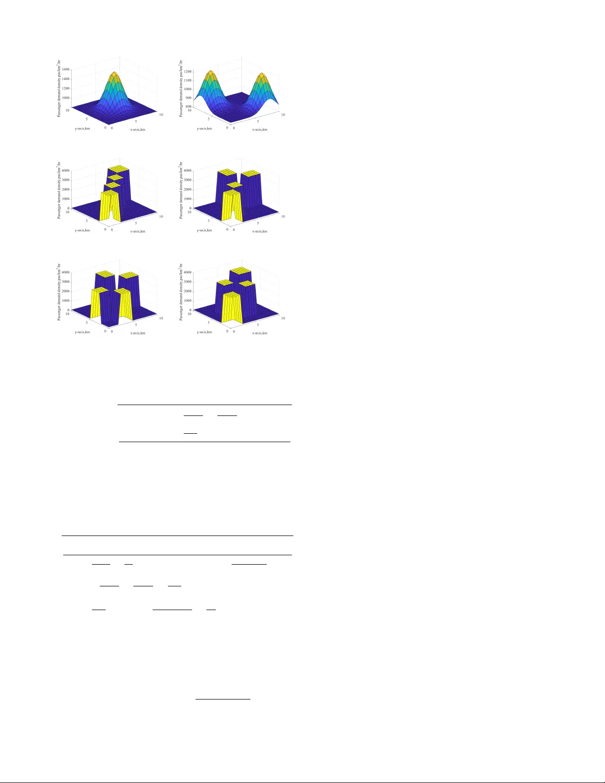
Design of T ransit Networks: Global Optimization of Continuous Approximation Models via Geometric Programming 1 st Haoyang Mao* Department of Electrical and Electr onic Engineering The Hong K ong P olytec hnic University Hong Kong, PR China hyang.mao@connect.polyu.hk 2 nd W eihua Gu Department of Electrical and Electr onic Engineering The Hong K ong P olytec hnic University Hong Kong, PR China weihua.gu@polyu.edu.hk 3 rd W enbo Fan Department of Electrical and Electr onic Engineering The Hong K ong P olytec hnic University Hong Kong, PR China wenbo.fan@polyu.edu.hk 4 th Zhicheng Jin Department of Electrical and Electr onic Engineering The Hong K ong P olytec hnic University Hong Kong, PR China zhicheng.jin@connect.polyu.hk 5 th Xiaokuan Zhao Department of Electrical and Electr onic Engineering The Hong K ong P olytec hnic University Hong Kong, PR China xiaokuan98.zhao@connect.polyu.hk Abstract —Continuous approximation (CA) models hav e been widely adopted in transit network design studies due to their strong analytical tractability and high computational efficiency . Howev er , such models are typically formulated as nonconv ex optimization problems, and existing solution approaches mainly rely on iterative algorithms that exploit first-order optimality information or nonlinear programming solvers, whose solution quality lacks stability guarantees under complex demand condi- tions. This paper proposes a geometric programming (GP)–based CA method for transit network design , which can be effi- ciently solved to global optimality . Numerical experiments are conducted on both homogeneous and heterogeneous network settings to evaluate the effectiveness of the proposed approach. Comprehensi ve tests are perf ormed under the combinations of six heterogeneous demand distrib utions, four levels of total passenger demand, and three value-of-time parameters. The results indicate that the GP approach consistently outperforms the coordinate descent method across all test cases, achieving cost reductions of approximately 1%–4%, e ven when the latter conv erges to identical solutions under different initializations. In comparison, nonlinear pr ogramming solvers, with fmincon as a representati ve example, are able to obtain globally optimal solutions comparable to those of the GP approach in low-demand heterogeneous networks; however , their performance becomes unstable under high-demand conditions. These findings demonstrate that GP pro vides an efficient and rob ust optimization framework for solving CA–based transit network design problems, especially in high-demand and highly heter ogeneous netw ork en vir onments. Index T erms —T ransit network design, Continuum approxima- This research is supported by the Natural Science Foundation of China (NSFC, Grant No. 725B2037). * Haoyang Mao is the corresponding author . tion, Geometric programming I . I N T RO D U C T I O N T ransit networks constitute the backbone of urban public transportation systems and play a critical role in both residents’ trav el ef ficiency and the operational costs of public transit services. W ith the increasing complexity of tra vel demand patterns, traditional optimization approaches based on dis- crete network flo w models hav e rev ealed inherent limitations when addressing large-scale transit netw ork design problems, most notably the NP-hard and curse of dimensionality . These methods often struggle to strike an effecti ve balance between computational tractability and solution quality . Against this backdrop, the continuous approximation (CA) approach has gradually emerged as an important theoretical framew ork for transit network design and optimization due to its strong analytical tractability and high computational efficiency . The fundamental idea of CA is to transform discrete el- ements—such as lines, stops, and origin–destination (OD) demand matrices—into continuous representations of density per unit area, expressed as functions of time and space [1], [2]. This transformation not only substantially reduces com- putational complexity but also enables a systematic deriv ation of analytical relationships between network design parameters and system performance measures. As a result, CA-based models provide transit planners with theoretical insights that are both interpretable and policy-rele vant. Howe ver , the frameworks of these studies are typically for- mulated as nonlinear programming (NLP) problems with non- con vex objectiv e functions and constraints. Existing solution approaches largely rely on iterativ e algorithms that exploit first-order optimality information, such as gradient descent and coordinate descent methods [2]–[4], or general-purpose nonlinear optimization solvers (e.g., fmincon) [5], [6]. These methods suffer from shortcomings. On the one hand, gradient- based algorithms, while offering numerical stability , are highly susceptible to local optima and thus cannot guarantee solution quality . On the other hand, general NLP solv ers often exhibit pronounced instability , with solution quality being highly sensitiv e to the choice of initial points. The difficulty of ob- taining reliable globally optimal solutions has, to some extent, hindered the broader practical application of CA methods in transit network design. T o o vercome these challenges, this paper introduces geomet- ric programming (GP) as an optimization paradigm, which is a specialized optimization technique tailored for problems with posynomial structures. Its core theoretical foundation lies in the fact that, through exponential variable substitutions and logarithmic transformations, a non-con vex problem can be equiv alently con verted into a con vex optimization problem. This transformation enables the use of efficient interior -point methods to obtain globally optimal solutions in polynomial time, without requiring any initial solution guesses [7]. Impor- tantly , this process preserves the physical interpretation of the original v ariables while pro viding strong theoretical guarantees of global optimality . GP has been successfully applied in various engineering fields, including communication networks [8], integrated cir- cuit design [9], and natural gas infrastructure networks [10], demonstrating its unique advantages in handling large-scale optimization problems with multiple constraints. Howe ver , to the best of the authors’ knowledge, the application of GP to CA models for transit network design has not yet been reported in the literature. This methodological gap constitutes the primary motivation of the present study . In summary , this study makes the following contributions: • The classical CA models for transit network design are solved through GP , thereby providing a solution paradigm with guaranteed global optimality . • Extensiv e numerical experiments are conducted under both homogeneous and heterogeneous networks, and the proposed GP-based approach is compared with gradient- based algorithms and commonly used nonlinear program- ming solvers. The paper unfolds as follows: Section 2 presents the CA modeling framew ork for homogeneous and heterogeneous network design problems, and section 3 shows the solution approach via GP . Section 4 describes the numerical case stud- ies. Section 5 summarizes the findings and outlines directions for future research. I I . O P T I M A L N E T W O R K D E S I G N M O D E L This study considers a square city as the study area and constructs both homogeneous and heterogeneous grid-based transit networks, as illustrated in Fig. 1. The study area is denoted by R , with a side length of | R | . A location within R is represented by the two-dimensional vector ( x, y ) , where x, y ∈ [0 , | R | ] . Model variables and parameters are labeled by operational direction i ∈ I , where set I includes E (Eastbound), W (W estbound), N (Northbound), and S (Southbound), respectively . In a homogeneous network, the line density and service headway in each operational direction are assumed to be constant o ver the entire study area R . In contrast, the het- erogeneous network considered in this study , following Chien and Schonfeld (1997) [2], allo ws the line density and service headway in each direction i ∈ I = { E , W , N , S } to vary spatially in the direction perpendicular to the line orientation, while remaining in variant along the line direction Moreover , no lateral detours in the perpendicular direction are permitted in the heterogeneous network. The model parameters are distinguished between spatially varying (localized) quantities and spatially in v ariant parame- ters. T o establish a unified modeling framew ork applicable to both homogeneous and heterogeneous networks, the localized parameters are formulated as functions of the spatial coor- dinates ( x, y ) . All parameters are summarized in Appendix A. The model is subsequently simplified in Section II-D according to the characteristics of each network type. Ｎ／Ｓ ｌｉｎｅｓ Ｎ 个 Ｅ／Ｗ ｌｉｎｅｓ Ｗ← ＳＩＸｅ－ →Ｅ Ｘ－ａｘ１Ｓ 个Ｓ (a) Homogeneous network Ｎ／Ｓ ｌｉｎｅｓ Ｎ 个 Ｅ／Ｗ ｌｉｎｅｓ Ｗ← ｙ－ａＸＩＳ 个Ｓ →Ｅ Ｘ－ａｘ１Ｓ (b) Heterogeneous network Fig. 1. Illustration of homogeneous and heterogeneous grid-based transit networks in a square city . A. Basic concepts and assumptions The model in volves two cate gories of decision variables: the line density δ i ( x, y ) and the service headway h i ( x, y ) . The former determines the structural configuration of the transit network, while the latter governs the operational characteris- tics of transit vehicles. Reflecting real-world practice, most transit lines operate in bidirectional symmetry . Accordingly , we assume δ E ( x, y ) = δ W ( x, y ) , δ N ( x, y ) = δ S ( x, y ) ; and h E ( x, y ) = h W ( x, y ) , h N ( x, y ) = h S ( x, y ) , so as to reduce operational complexity . Regarding stop placement, all stops are assumed to be located at the intersections of any two perpendicular transit lines. P assengers are allo wed to transfer between orthogonal lines at these stops, and vehicles are assumed to operate without skip-stop service. Intermediate stops between adjacent transfer stops are neglected in this study and are left for future in vestigation. Based on the two categories of decision variables, the vehicle flo w of lines in direction i per unit cross-sectional distance in the network, denoted by q i ( x, y ) , can be computed as shown in Eq. (1): q i ( x, y ) = δ i ( x, y ) h i ( x, y ) , i ∈ I , x, y ∈ [0 , | R | ] (1) Passenger demand density is treated as an exogenous input to the model and is denoted by λ i ( x o , y o , x d , y d ) , which is a function of four spatial coordinates. Here, ( x o , y o ) and ( x d , y d ) represent the origin and destination of the passenger, respectiv ely . W ith respect to their travel behavior , following previous studies [11]–[14], the following assumptions are adopted: • Passengers walk to the nearest transit stops for boarding and alighting. • Passengers arri ve at the origin stop randomly , without consulting the transit schedule. • Passenger service follo ws the first-in, first-served (FIFS) principle, since passenger flows do not exceed the service capacity provided by the vehicle flows in any direction i at any location ( x, y ) in the network (see the constraint formulation in Section II-C). Under these assumptions, the high-dimensional passenger demand density function can be aggregated to construct sev- eral categories of demand functions, including the board- ing passenger density λ i bo ( x, y ) , alighting passenger density λ i al ( x, y ) , on-board flux density λ i f l ( x, y ) , and transferring density λ i tr ( x, y ) . The detailed deriv ation of these quantities follows the methodology proposed by Chien and Schonfeld (1997) [2]. B. Network design objective function The total system cost of the transit network is denoted by Z , which consists of two components: the agenc y cost ( Z A ) and the passenger cost ( Z P ). The computation of the system cost is given in Eq. (2), where µ represents passengers’ av erage value of time (V O T). Z = 1 µ Z A + Z P (2) Agency cost, Z A , comprises four metrics: (i) the line infrastructure length, N l ; (ii) the number of stops, N s ; (iii) the vehicle distance trav eled, N k ; and (iv) the vehicle time trav eled, N h . Follo wing Daganzo and Ouyang (2019) [12], Z A is computed as shown in Eq. (3), where the parameters π l , π s , π k , and π h denote unit costs associated with the four metrics, ¯ i represents the direction perpendicular to direction i , v denotes cruising speed of transit vehicles, and τ is the fixed delay per stop. Z A = π l N l + π s N s + π k N k + π h N h , (3a) N l = X i ∈ I Z | R | y =0 Z | R | x =0 δ i ( x, y ) dx dy , (3b) N s = X i ∈ I Z | R | y =0 Z | R | x =0 δ i ( x, y ) δ ¯ i ( x, y ) dx dy , (3c) N k = X i ∈ I Z | R | y =0 Z | R | x =0 q i ( x, y ) dx dy , (3d) N h = X i ∈ I Z | R | y =0 Z | R | x =0 q i ( x, y )  1 v + τ δ ¯ i ( x, y )  dx dy . (3e) Equations (3b) and (3d) are straightforward, as they can be computed by integrating the corresponding density functions ov er the study area R . As discussed in Section II-A, stops are assumed to be located at the intersections of an y two perpen- dicular transit lines. Accordingly , the term δ i ( x, y ) δ ¯ i ( x, y ) in Eq. (3c) provides an estimate of the stop density at location ( x, y ) , and the resulting stop density is identical for all four operational directions. Equation (3e) consists of cruising time and dwell time at stops. Passenger cost, Z P , is characterized by four primary met- rics: (i) the access/egress time, T a ; (ii) the out-of-vehicle wait time, T w ; (iii) the in-vehicle ride time, T r ; and (iv) the transfer penalty , T t . It should be noted that fare payments are excluded from the system cost, as the y represent transfers between passengers and the transit agency and therefore cancel out at the system le vel. Z P is formulated in Eq. (4), where v w denotes the walking speed of passengers, and σ represents the transfer penalty . Additionally , walking time is multiplied by a perceiv ed walking time factor β w , reflecting the higher perceiv ed cost of w alking relati ve to in-vehicle trav el [15]. Z P = T a + T w + T r + T t , (4a) T a = β w X i ∈ I Z | R | 0 Z | R | 0  λ i bo ( x, y ) + λ i al ( x, y )  ×  1 4 v w δ i ( x, y ) + 1 4 v w δ ¯ i ( x, y )  dx dy , (4b) T w = X i ∈ I Z | R | y =0 Z | R | x =0  λ i bo ( x, y ) + λ i tr ( x, y )  h i ( x, y ) 2 dx dy , (4c) T r = X i ∈ I Z | R | y =0 Z | R | x =0 λ i f l ( x, y )  1 v + τ δ ¯ i ( x, y )  dx dy , (4d) T t = σ X i ∈ I Z | R | y =0 Z | R | x =0 λ i tr ( x, y ) dx dy . (4e) Equation (4b) estimates passengers’ access and egress time using numerical integration, where 1 δ i ( x,y ) represents the spacing between transit lines in direction i at location ( x, y ) . Equation (4c) accounts for the total waiting time, including both initial waiting and transfer waiting. Equation (4d) captures passengers’ in-vehicle trav el time, consisting of cruising time and dwell time at stops. Finally , Equation (4e) directly integrates the transfer density and multiplies it by the corresponding penalty time. C. Model constr aints The model is subject to tw o primary sets of constraints. First, in any direction i at any location ( x, y ) within the study area R , the passenger flow must not exceed the maximum service capacity provided by the corresponding vehicle flow , as expressed in Eq. (5), where C denotes the capacity of a transit vehicle. λ i f l ( x, y ) q i ( x, y ) ≤ C , i ∈ I , x, y ∈ [0 , | R | ] (5) Second, non-negativity constraints are imposed on the decision variables to ensure their physical interpretability . Moreov er, since both δ i ( x, y ) and h i ( x, y ) appear in the denominator of certain terms in the model formulation, the y are further restricted to be strictly positiv e. The resulting constraints are giv en by δ i ( x, y ) , h i ( x, y ) > 0 , i ∈ I , x, y ∈ [0 , | R | ] (6) D. Model specialization for heter og eneous and homogeneous networks For heterogeneous networks, the two categories of decision variables in each direction i ∈ I = { E , W, N , S } are assumed to remain in variant along the corresponding line direction. In addition, considering the bidirectional symmetry of the transit network, they can be specified as: δ i ( x, y ) = ( δ E W ( y ) , i ∈ { E , W } δ N S ( x ) , i ∈ { N , S } (7) Under this specification, δ E W ( y ) , and δ N S ( x ) are treated as the new decision variables. The same specialization applies to the service headway h i ( x, y ) . The objectiv e function must be inte grated along the di- rection of operation for each i ∈ I = { E , W , N , S } . T ak- ing Eq. (3e) as an example, the resulting expression after integration is given by Eq. (8), where q E W ( y ) = δ E W ( y ) h E W ( y ) , and q N S ( x ) = δ N S ( x ) h N S ( x ) . The transformations of the remaining objectiv e function terms in Eqs. (3) and (4) follow the same procedure and are therefore omitted for brevity . N h = 2 Z | R | y =0 q E W ( y ) | R | v + τ Z | R | x =0 δ N S ( x ) dx ! dy + 2 Z | R | x =0 q N S ( x ) | R | v + τ Z | R | y =0 δ E W ( y ) dy ! dx (8) Under the above specialization, the capacity constraint in Eq. (5) for directions E , W can be reformulated as Eq. (9). The corresponding expressions for directions N , S follow analogously .        λ E W f l ( y ) q E W ( y ) ≤ C λ E W f l ( y ) = max i ∈{ E ,W } ,x ∈ [0 , | R | ] λ i f l ( x, y ) , y ∈ [0 , | R | ] (9) For homogeneous netw orks, the two cate gories of deci- sion v ariables in each operational direction are assumed to be constant over the entire study area R . Consequently , δ E W , δ N S , h E W , and h N S are treated as the new decision variables. The objective function is then integrated over all directions. T aking Eq. (3e) as an example, the corresponding expression is presented in Eq. (10), where q E W = δ E W h E W , and q N S = δ N S h N S . N h = | R | 2  q E W  1 v + τ δ N S  + q N S  1 v + τ δ E W  (10) The capacity constraint in Eq. (5) takes the form of Eq. (11) for directions E , W ; an identical form applies to directions N , S .        λ E W f l q E W ≤ C λ E W f l = max i ∈{ E ,W } ,x,y ∈ [0 , | R | ] λ i f l ( x, y ) (11) I I I . S O L U T I O N M E T H O D V I A G E O M E T R I C P R O G R A M M I N G GP is a class of nonlinear and noncon v ex optimization problems that possesses a number of attractiv e theoretical and computational properties. A ke y advantage of GP lies in the fact that it can be transformed into an equi valent con ve x optimization problem through a suitable change of v ariables. As a result, global optimal solutions can be computed ef- ficiently without reliance on initial guesses. Interior-point methods dev eloped for GP are known to admit polynomial- time complexity guarantees [16]. A brief overvie w of GP follo ws. GP admits two equiv alent representations: a standard (posynomial) form and a conv ex form obtained via logarithmic transformation. The standard form is expressed in terms of a special class of functions known as monomials and posynomials. A monomial is defined as a function g : R n ++ → R , shown as Eq. (12), where d ≥ 0 is a multiplicativ e constant coefficient, and a ( l ) ∈ R , l = 1 , 2 , ... L are real-valued exponents. g ( r ) = d r a (1) 1 r a (2) 2 ... r a ( L ) L , r > 0 (12) A posynomial is defined as a finite sum of monomials, presented in Eq. (13), where k = 1 , 2 , ... K is the index of the monomial. For e xample, expressions such as ln 2 · r π 1 r − 100 2 + r 2 r 4 3 constitute posynomials, whereas expressions in volving sub- traction (e.g., r 1 − r 2 ) do not, due to the nonnegati vity requirement on multiplicativ e coef ficients. f ( r ) = K X k =1 d k r a (1) k 1 r a (2) k 2 ... r a ( L ) k L , r > 0 (13) In its standard form, a GP minimizes a posynomial objective subject to posynomial inequality constraints and monomial equality constraints, all normalized to unity: min r f 0 ( r ) , s.t. f u ( r ) ≤ 1 , u = 1 , 2 , ..., U , g w ( r ) = 1 , w = 1 , 2 , ..., W , r > 0 . (14) Although this formulation is not conv ex—since posynomi- als are generally noncon ve x functions—the problem can be equiv alently transformed into a con ve x program by apply- ing a logarithmic change of variables. Specifically , defining s l = ln r l , b uk = ln d uk , b w = ln d w and taking logarithms of the objective and constraints yields the con vex form of GP: min s ln f 0 ( s ) = ln K 0 X k =1 e ( a T 0 k s + b 0 k ) , s.t. ln f u ( s ) = ln K u X k =1 e ( a T uk s + b uk ) ≤ 0 , u = 1 , 2 , ..., U , ln g w ( s ) = a T w s + b w = 0 , w = 1 , 2 , ..., W , s ∈ R . (15) This formulation is a con vex optimization problem, as the log-sum-exp function is con vex [17]. In the proposed CA-based transit network design problem, the unified objectiv e functions in Eqs. (3) and (4) are explicitly formulated as posynomials of the two categories of decision variables, namely the line density δ i ( x, y ) and the service headway h i ( x, y ) . For the constant terms that are independent of the decision variables, such as Eq. (4e), they can be equiv alently represented as monomials with zero e xponents on the decision variables. The capacity constraint in Eq. (5) satisfies the requirement that inequality constraints in GP standard form must take a posynomial form. Moreover , Eq. (6) ensures that all decision variables are strictly positiv e, which is a fundamental assump- tion of GP . The specialization of the unified model to heterogeneous and homogeneous network settings inv olves only spatial in- tegration and v ariable aggregation, and does not alter the posynomial structure of the objective function or the con- straints. Consequently , the resulting optimization problems for both network types conform to the standard form of GP . Therefore, the problem is solv ed using the commercial GP solver MOSEK on a desktop computer with a 2.5 GHz CPU (Intel(R) i5-12500H) and a 16G memory , which ef ficiently yields the global optimum. I V . N U M E R I C A L C A S E S T U D I E S A. Set-up In this section, the proposed models and solution approach are primarily demonstrated using a grid-based city with an area of 10 × 10 k m 2 . For computational tractability , the city is discretized into uniform square cells of size ∆ 2 . Each cell is represented by its center point ( x n , y n ′ ) , where n, n ′ = 1 , 2 , ..., N = | R | ∆ . All density functions and service headway within a cell are assumed to be spatially homogeneous and equal to their values at the corresponding cell center . T o comprehensiv ely assess the rob ustness and performance of the proposed method, numerical experiments are con- ducted for both homogeneous and heterogeneous networks under a wide range of scenarios. Specifically , six hetero- geneous demand distrib utions (monocentric, commute, and four chessboard-type patterns), four lev els of total passenger demand (5,000, 10,000, 50,000, and 100,000), and three values of passengers’ V O T ( 25 $ hr , 20 $ hr , 5 $ hr ) are considered, result- ing in a total of 72 test cases. The generation of heterogeneous demand distributions is detailed in Appendix B. The selected V O T v alues are intended to represent economic conditions in dev eloped, moderately dev eloped, and dev eloping regions. In addition, the globally optimal solutions obtained via GP are compared with those deri ved from gradient-based algorithms (represented by coordinate descent) and general- purpose nonlinear programming solvers (represented by fmin- con). F or the coordinate descent method, closed-form solutions for the two categories of decision variables are provided in Appendix C. Other parameter v alues are taken from Ouyang et al. (2014) [3], summarized in Appendix A. B. Numerical r esults T able I reports the average percentage reductions in total system cost achie ved by the GP model, relative to the two benchmark algorithms, across six demand distributions under giv en total demand lev els D and values of µ . Fig. 2 illustrates the per-passenger system cost and its individual cost compo- nents obtained using the GP approach, in comparison with the two benchmark algorithms. The numerical results demonstrate that the GP-based ap- proach consistently outperforms the two benchmark algo- rithms. Compared with the coordinate descent method, GP yields systematic reductions in total system cost, with im- prov ements ranging from approximately 1% to ov er 4%, indicating that coordinate descent often con verges to subopti- mal stationary points despite its stability across ten different initializations. When compared with the general-purpose nonlinear solver fmincon, GP still exhibits clear advantages in heterogeneous networks, particularly under high demand and lo w µ . For homogeneous networks, fmincon matches the GP solutionl, primarily because the problem inv olves only four decision variables, making the global optimum relati vely easy to iden- tify . In addition, fmincon was initialized from ten distinct starting points. For heterogeneous networks, in the same exper - imental setting, the resulting solutions exhibit non-ne gligible T ABLE I A V ER AG E R E L A T I VE O P TI M A LI T Y I M P ROV E ME N T ( % ) O F T H E G P A P PR OAC H A CR OS S S I X D E M AN D D I S T RI B U TI O N S F O R D I FF E RE N T T OTAL D E MA N D L E V EL S D A N D V A L UE S O F µ . D Solution method Coordinate descent fmincon µ = 25 µ = 20 µ = 5 µ = 25 µ = 20 µ = 5 Heter ogeneous network 5000 2.70 2.86 3.84 0.08 0.08 0.19 10000 2.21 2.37 3.35 0.13 0.11 0.27 50000 1.26 1.37 1.07 0.62 0.35 1.51 100000 0.89 0.87 0.67 0.94 1.12 2.48 Homogeneous network 5000 3.09 3.28 4.45 0.00 0.00 0.00 10000 2.51 2.69 3.76 0.00 0.00 0.00 50000 1.40 1.52 0.80 0.00 0.00 0.00 100000 0.81 0.58 0.50 0.00 0.00 0.00 Ｐｅｒ－ｐａｓｓｅｎｇｅｒ ｃｏｓｔ（ｍｉｎ） １２０ ３．８８％ ３．８３％ ３．８２％ ３．８５％ ３．８５％ ３．８２％ １０４．２４ １０５．３３ １０５．３９ １００．２０ １０１．３０ １０１．３５ １０４．７９ １００．７５ １０４．７９ １０５．３９ １００．７５ １０１．３５ １００ ８０ ６０ ４０ ２０ ０ ＣＤ ＧＰ ＣＤ ＧＰ ＣＤ ＧＰ ＣＤ ＧＰ ＣＤ ＧＰ ＣＤ ＧＰ Ｍｏｎｏｃｅｎｔｒｉｃ Ｃｏｍｍｕｔｅ Ｃｈｅｓｓｂｏａｒｄ１ Ｃｈｅｓｓｂｏａｒｄ２ Ｃｈｅｓｓｂｏａｒｄ３ Ｃｈｅｓｓｂｏａｒｄ４ Ｎｋ／μ Ｎｈ／μ Ｔａ Ｔｗ Ｔｒ Ｔｔ (a) Coordinate descent method (CD) with D = 5 , 000 passengers and µ = 5 $ hr Ｐｅｒ－ｐａｓｓｅｎｇｅｒ ｃｏｓｔ （ｍｉｎ） ２．５７％ ３．８７％ ３．１８％ ２．５５％ ７０ １．７７％ ０．９０％ ６８．４６ ６６．７０ ６８．８４ ６６．１８ ６８．４２ ６６．２４ ６８．４５ ６６．７１ ６１．３４ ６０．２５ ６２．４７ ６１．９０ ６０ ５０ ４０ ３０ ２０ １０ ０ ｆｍｉｎｃｏｎ ＧＰ ｆｍｉｎｃｏｎ ＧＰ ｆｍｉｎｃｏｎ ＧＰ ｆｍｉｎｃｏｎ ＧＰ ｆｍｉｎｃｏｎ ＧＰ ｆｍｉｎｃｏｎ ＧＰ Ｍｏｎｏｃｅｎｔｒｉｃ Ｃｏｍｍｕｔｅ Ｃｈｅｓｓｂｏａｒｄｌ Ｃｈｅｓｓｂｏａｒｄ２ Ｃｈｅｓｓｂｏａｒｄ３ Ｃｈｅｓｓｂｏａｒｄ４ Ｔｒ Ｔｗ Ｔａ Ｎｎ／μ Ｎｋ／μ Ｔｔ (b) Fmincon with D = 100 , 000 passengers and µ = 5 $ hr Fig. 2. Illustration of per-passenger system cost under six demand distribu- tions in heterogeneous network: GP approach vs. two benchmark algorithms. variability , with differences between the minimum and max- imum total system costs exceeding 10%. In such cases, the solution with the lowest total system cost was selected for comparison with the GP benchmark. This underscores the sensitivity and limited rob ustness of fmincon when applied to higher-dimensional, noncon vex formulations. Overall, these results highlight the robustness and efficienc y of the GP formulation in deli vering globally optimal solutions, especially for large-scale and highly heterogeneous transit network design problems. V . S U M M A RY A N D C O N C L U S I O N S This study applies GP to the CA–based transit network design problem, yielding solutions with guaranteed global op- timality . Numerical experiments demonstrate that con ventional gradient-based algorithms and general-purpose nonlinear pro- gramming solvers cannot consistently ensure solution quality as experimental conditions vary , ev en when con vergence is achiev ed from multiple initializations. In contrast, the GP- based approach provides a robust and reliable tool for large- scale transit network optimization. Nev ertheless, the applicability of GP is constrained by its stringent requirements on posynomial objectiv e and constraint structures, which limit its broader use in CA-based transit net- work design. Future research may explore extensions such as sequential geometric programming (SGP), signomial geomet- ric programming, or mixed-inte ger geometric programming (MIGP), le veraging con vex approximations and relaxations to expand the applicability of GP-based methods in this domain. A P P E N D I X A. Nomenclatur e In this appendix, we summarize all model variables and parameters used in the study . T able II provides the symbols of the model variables, along with their definitions, units, and corresponding values. B. Heter ogeneous demand distrib ution gener ation For the monocentric and commute demand distributions, we follow the method outlined by Ouyang et al. (2014) [3], as described in Eq. (16), where D represents the total passenger demand. The parameter values in Eq. (16a) are provided in T able III. Eq. (16b) scales the demand density function proportionally based on the given D . The generated results are shown in Figs. 3(a) and 3(b). λ ′ ( x o , y o , x d , y d ) = Y θ = o,d " α 1 + α 2 2 X γ =1 e − ( α 3 γ x θ − β θγ ) 2 − ( α 4 γ x θ − ¯ β θγ ) 2 # , (16a) λ ( x o , y o , x d , y d ) = D R RR R | R | 0 λ ′ ( x o , y o , x d , y d ) dx o dy o dx d dy d λ ′ ( x o , y o , x d , y d ) . (16b) T o further enhance the heterogeneity of passenger demand distribution, we propose a chessboard demand distribution. The core idea is to divide the network into high-density H and low-density L re gions, which are distrib uted in a chessboard- like pattern across the network. The passenger demand density remains constant within each H and L re gion. The higher heterogeneity of this pattern arises from the asymmetric distri- bution of tra vel origins and destinations, which may f acilitate a more realistic design. The design process for this demand distribution consists of three steps: 1) Identifying the locations of each H and L regions. T ABLE II S U MM A RY O F M O D EL V A RI A B L ES A ND PAR A M E TE R S . Decision variables Description δ i ( x, y ) Line density in direction i ∈ I at location ( x, y ) ( 1 km ). h i ( x, y ) Headway in direction i ∈ I at location ( x, y ) ( hr veh ). Other variables q i ( x, y ) V ehicle flow in direction i ∈ I at location ( x, y ) ( veh hr · k m ). Z, Z A , Z P Objectiv e metrics: total system cost ( hr ), Agency cost ( $ ), Passenger cost ( hr ). N l , N s , N k , N h Agency metrics: line infrastructure length ( k m ), number of stops, vehicle distance tra veled ( veh · k m hr o ), vehicle time traveled ( veh · hr hr o ). T a , T w , T r , T t Passenger metrics: access/egress cost ( hr ), wait time ( hr ), in-vehicle travel time ( hr ), transfer penalty ( hr ). Model parameters π l , π s , π k , π h Unit cost of line infrastructure length ( 0 $ km ), num- ber of stops ( 0 $ ), vehicle-kilometers ( 2 $ veh · k m ), vehicle-hours ( 40 $ veh · hr ). λ ( x o , y o , x d , y d ) Passenger demand density with origin at ( x o , y o ) and destination at ( x d , y d ) ( pas km 4 · hr o ). λ i bo ( x, y ) Boarding passenger density in direction i ∈ I at location ( x, y ) ( pas km 2 · hr o ). λ i al ( x, y ) Alighting passenger density in direction i ∈ I at location ( x, y ) ( pas km 2 · hr o ). λ i f l ( x, y ) On-board flux density in direction i ∈ I at location ( x, y ) ( pas km · hr o ). λ i tr ( x, y ) T ransferring density in direction i ∈ I at location ( x, y ) ( pas km 2 · hr o ). v Cruising speed of transit vehicles ( 25 km hr ). v w W alking speed of passengers ( 2 km hr ). C Capacity of a transit vehicle ( 80 pas veh ). D T otal Passenger demand ( 5 , 000 , 10 , 000 , 50 , 000 , 100 , 000 pas ). µ Passengers’ average V OT ( 25 , 20 , 5 $ hr ). β w Perceiv ed walking time factor of passengers (2) τ Fixed delay per stop ( 30 3600 hr ). σ T ransfer penalty ( 60 3600 hr ). ∆ Discretization parameter ( 0 . 5 k m ). 1 hr denotes the time unit of hours, and hr o denotes the operating time of a transit system. 2 For each variable and parameter , the parentheses specify the unit and, where applicable, the numerical value used in the case studies. T ABLE III P A R A M ET E R S O F T H E D E M AN D D E N S IT Y F U N C TI O N F O R M O NO C E N TR I C A N D C O M M UT E PA T T E RN S . Demand α 1 α 2 α 31 α 32 α 41 α 42 β o 1 Monocentric 0.0016 0.065 0.5 0 0.5 0 2.5 Commute 0.00044 0.70 0.5 0 0.5 0 1.0 Demand β o 2 β d 1 β d 2 ¯ β o 1 ¯ β 2 ¯ β d 1 ¯ β d 2 Monocentric 0 2.5 0 2.5 0 2.5 0 Commute 0 4.0 0 4.0 0 1.0 0 2) Constructing passenger transfer equation set to solve for demand densities in the four transfer scenarios: high- density to high-density , λ H → H ; high-density to low- density , λ H → L ; low-density to high-density , λ L → H ; and low-density to low-density , λ L → L . The equation set is gi ven in Eq. (17), where Eq. (17a) calculates the departure and arriv al demand densities, and Eq. (17b) constrains the total demand and relev ant ratios. R H and R L represent the areas of high and low demand re gions, respecti vely . λ bo,H and λ bo,L denote the demand densities lea ving the high- and lo w-density regions, while λ al,H and λ al,L represent the demand densities arriving in these re gions. ρ H is the proportion of demand leaving and arriving in high-density areas, and ρ H → H is the proportion of demand within high- density regions that corresponds to the H → H transfer scenario. In this study , both of these ratios are set to 0.9.          λ bo,H = R H λ H → H + R L λ H → L λ bo,L = R H λ L → H + R L λ L → L λ al,H = R H λ H → H + R L λ L → H λ al,L = R H λ H → L + R L λ L → L (17a)                R H λ bo,H + R L λ bo,L = D R H λ al,H + R L λ al,L = D R H λ bo,H D = R H λ al,H D = ρ H R H λ H → H λ bo,H = ρ H → H (17b) The solution is given in Eq. (18). Notably , λ H → L = λ L → H , as R H λ bo,H D = R H λ al,H D = ρ H .                  λ H → H = D ρ H R 2 H (2 − ρ H → H ) λ H → L = λ L → H = D ρ H (1 − ρ H → H ) R H R L (2 − ρ H → H ) λ L → L = D (2 − ρ H → H − 3 ρ H + 2 ρ H ρ H → H ) R 2 L (2 − ρ H → H ) (18) 3) Assigning v alues to λ ( x o , y o , x d , y d ) based on the results from step 2) and the locations determined in step 1). Finally , we obtained four distinct chessboard demand dis- tributions, as sho wn in Figs. 3(c), 3(d), 3(e), and 3(f). C. Coor dinate descent algorithm for model solution For heterogeneous networks, the solution procedure is sum- marized as follow . First, initial values of decision v ariable δ (0) E W ( y n ′ ) , δ (0) N S ( x n ) , h (0) E W ( y n ′ ) , h (0) N S ( x n ) are randomly generated. Second, holding the line densities δ fixed, the unconstrained optimal headways are obtained by solving the first-order optimality conditions of the total cost function. For the E , W direction, the candidate headway at iteration m is gi ven by Ｐａｓｓｅｎｇｅｒ ｄｅｍａｎｄ ｄｅｎｓｔｙ，ｐａｓ／ｋｍ２／ｈｒ １６００ １４００ １２００ １０００ １０ ５ ５ ｙ－ａｘｉｓ，ｋｍ ００ Ｘ－ａｘｉｓ，ｋｍ １０ (a) Monocentric demand Ｐａｓｓｅｎｇｅｒ ｄｅｍａｎｄ ｄｅｎｓｔｙ，ｐａｓ／ｋｍ２／ｈｒ １２００ １１００ １０００ ９００ ８００ １０ ５ ５ ００ ｙ－ａｘｉｓ，ｋｍ １０ Ｘ－ａｘｉｓ，ｋｍ (b) commute demand Ｐａｓｓｅｎｇｅｒ ｄｅｍａｎｄ ｄｅｎｓｔｙ，ｐａｓ／ｋｍ２／ｈｒ ４０００ ３０００ ２０００ １０００ ０ １０ ５ ５ ００ ｙ－ａｘｉｓ，ｋｍ Ｘ－ａｘｉｓ，ｋｍ １０ (c) Chessboard1 demand Ｐａｓｓｅｎｇｅｒ ｄｅｍａｎｄ ｄｅｎｓｔｙ，ｐａｓ／ｋｍ２／ｈｒ ４０００ ３０００ ２０００ １０００ ０ １０ ５ ５ ｙ－ａｘｉｓ，ｋｍ ００ Ｘ－ａｘｉｓ，ｋｍ １０ (d) Chessboard2 demand Ｐａｓｓｅｎｇｅｒ ｄｅｍａｎｄ ｄｅｎｓｔｙ，ｐａｓ／ｋｍ２／ｈｒ ４０００ ３０００ ２０００ １０００ ０ １０ ５ ５ ００ ｙ－ａｘｉｓ，ｋｍ １０ Ｘ－ａｘｉｓ，ｋｍ (e) Chessboard3 demand Ｐａｓｓｅｎｇｅｒ ｄｅｍａｎｄ ｄｅｎｓｔｙ，ｐａｓ／ｋｍ２／ｈｒ ４０００ ３０００ ２０００ １０００ ０ １０ ５ ５ ｙ－ａｘｉｓ，ｋｍ ００ Ｘ－ａｘｉｓ，ｋｍ １０ (f) Chessboard4 demand Fig. 3. Sum of origin and destination demand densities ( D = 50 , 000 ). ˜ h ( m ) E W ( y n ′ ) = v u u u u u t 2 δ ( m − 1) E W ( y n ′ ) π k | R | µ + π h | R | µv + π h τ µ ∆ P N n =1 δ ( m − 1) N S ( x n ) ! ∆ P N n =1  λ E W bo ( x n , y n ′ ) + λ E W al ( x n , y n ′ )  (19) Third, with the headways h fixed, the optimal line densities are analogously derived from the corresponding first-order conditions. The expression for the E , W direction is δ ( m ) E W ( y n ′ ) = v u u u u u u u u u u u t ω w ∆ P N n =1 P i ′ = { E W ,N S }  λ i ′ bo ( x n , y n ′ ) + λ i ′ al ( x n , y n ′ )  4 v w        π l | R | µ + π s µ ∆ P N n =1 δ ( m − 1) N S ( x n ) + 1 ˜ h ( m ) E W ( y n ′ ) ×  π k | R | µ + π h | R | µv + π h τ µ ∆ P N n =1 δ ( m − 1) N S ( x n )  + τ π h µ ∆ P N n =1  δ ( m − 1) N S ( x n ) ˜ h ( m ) N S ( x n ) + µ π h λ N S f l ( x n , y n ′ )         (20) Fourth, to ensure that the capacity constraint is satisfied, the headways are updated accordingly . T aking the E , W direction as an example, the feasible headway is obtained as h ( m ) E W ( y n ′ ) = min ( ˜ h ( m ) E W ( y n ′ ) , C · δ ( m ) E W ( y n ′ ) λ E W f l ( y n ′ ) ) (21) Finally , Steps 2-4 are repeated until conv ergence is achiev ed, which typically occurs within approximately ten iterations. For homogeneous networks, the same coordinate descent framew ork applies; howe ver , due to space limitations, the detailed deriv ation is omitted. R E F E R E N C E S [1] E. M. Holroyd, “THE OPTIMUM BUS SER VICE: A THEORETICAL MODEL FOR A LARGE UNIFORM URBAN AREA, ” in Pr oceedings of the Third International Symposium on the Theory of Tr affic FlowOp- erations Researc h Society of America , 1967. [2] S. Chien and P . Schonfeld, “Optimization of Grid T ransit System in Heterogeneous Urban Environment, ” Journal of T ransportation Engi- neering , vol. 123, no. 1, pp. 28–35, 1997. [3] Y . Ouyang, S. M. Nourbakhsh, and M. J. Cassidy , “Continuum approx- imation approach to bus network design under spatially heterogeneous demand, ” T ransportation Resear ch P art B: Methodological , vol. 68, pp. 333–344, 2014. [4] H. Chen, W . Gu, M. J. Cassidy , and C. F . Daganzo, “Optimal transit service atop ring-radial and grid street networks: A continuum approxi- mation design method and comparisons, ” T ransportation Researc h P art B: Methodological , vol. 81, pp. 755–774, 2015. [5] L. Wu, W . Gu, W . Fan, and M. J. Cassidy , “Optimal design of transit networks fed by shared bikes, ” T ransportation Researc h P art B: Methodological , vol. 131, pp. 63–83, 2020. [6] L. Zhen, W . Gu, and X. Zhao, “Comparing skip-stop and all-stop transit network designs, ” T ransportation Research P art C: Emerging T echnologies , vol. 176, p. 105149, 2025. [7] M. A vriel, Ed., Advances in Geometric Progr amming . Boston, MA: Springer US, 1980. [8] M. Chiang, C. W . T an, D. P . Palomar , D. O’neill, and D. Julian, “Power Control By Geometric Programming, ” IEEE T ransactions on W ir eless Communications , vol. 6, no. 7, pp. 2640–2651, 2007. [9] S. P . Boyd, S.-J. Kim, D. D. Patil, and M. A. Horowitz, “Digital Cir- cuit Optimization via Geometric Programming, ” Operations Research , vol. 53, no. 6, pp. 899–932, 2005. [10] S. Misra, M. W . Fisher, S. Backhaus, R. Bent, M. Chertkov , and F . Pan, “Optimal Compression in Natural Gas Networks: A Geometric Programming Approach, ” IEEE T ransactions on Contr ol of Network Systems , vol. 2, no. 1, pp. 47–56, 2015. [11] C. Chriqui and P . Robillard, “Common Bus Lines, ” Tr ansportation Science , vol. 9, no. 2, pp. 115–121, 1975. [12] C. F . Daganzo and Y . Ouyang, “Public transportation systems: Principles of system design, operations planning and real-time control, ” in Public T ransportation Systems . WORLD SCIENTIFIC, 2019. [13] W . F an, Y . Mei, and W . Gu, “Optimal design of intersecting bimodal transit networks in a grid city , ” T ransportation Resear ch P art B: Method- ological , vol. 111, pp. 203–226, 2018. [14] Zhicheng Jin, Haoyang Mao, Di Chen, Hao Li, Huizhao T u, Ying Y ang, and Maria Attard, “Multi-objective optimization model of autonomous minibus considering passenger arriv al reliability and trav el risk, ” Com- munications in T ransportation Researc h , vol. 4, p. 100152, 2024. [15] M. W ardman, “ A revie w of British evidence on time and service quality valuations, ” T ransportation Researc h P art E: Logistics and T ransporta- tion Review , vol. 37, no. 2, pp. 107–128, 2001. [16] Y . Nesterov and A. Nemirovskii, Interior-P oint P olynomial Algorithms in Con vex Progr amming , ser . Studies in Applied and Numerical Math- ematics. Society for Industrial and Applied Mathematics, 1994. [17] S. Boyd and L. V andenberghe, Conve x Optimization . Cambridge Univ ersity Press, 2004.