Learning Lineage-guided Geodesics with Finsler Geometry

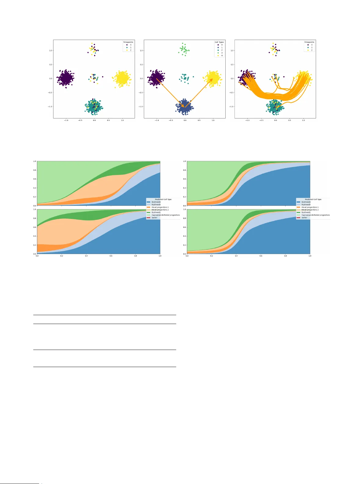
Learning Lineage-guided Geodesics with Finsler Geometry Aaron Zweig * 1,2 Mingxuan Zhang * 2,3 David A. Kno wles 1,3,4 Elham Azizi 2,3,4,5,6 1 New Y ork Genome Center 2 Irving Institute for Cancer Dynamics, Columbia Univ ersity 3 Department of Systems Biology , Columbia Univ ersity 4 Department of Computer Science, Columbia Univ ersity 5 Department of Biomedical Engineering, Columbia Univ ersity 6 Data Science Institute, Columbia Univ ersity Abstract T rajectory inference in vestigates how to interpolate paths between observed timepoints of dynamical systems, such as temporally resolved population distributions, with the goal of inferring trajecto- ries at unseen times and better understanding sys- tem dynamics. Previous w ork has focused on con- tinuous geometric priors, utilizing data-dependent spatial features to define a Riemannian metric. In many applications, there exists discrete, directed prior kno wledge ov er admissible transitions (e.g. lineage trees in developmental biology). W e in- troduce a Finsler metric that combines geometry with classification and incorporate both types of priors in trajectory inference, yielding improv ed performance on interpolation tasks in synthetic and real-world data. 1 INTR ODUCTION In many scientific domains, data are observed at discrete timepoints while the underlying system e volv es continu- ously in time. T rajectory inference aims to reconstruct con- tinuous paths between empirical distributions, enabling in- terpolation to unseen times and analysis of system e volution. Single-cell omics provides a prominent instance of this set- ting. Although single-cell RN A sequencing is destructi ve, sampling at multiple timepoints enables a weakly temporal perspecti ve on the ev olution of cells, particularly in dev elop- mental settings where cell dif ferentiation is similar among all healthy embryos. Ho wev er, the inability to sample con- tinuously means a practitioner typically only has access to the cell distribution at a small number of timepoints. In the context of trajectory inference, optimal transport (O T) * These authors contributed equally . Preprint is a popular modeling frame work across applications be- cause it follows the principle of minimal ener gy , where the inferred trajectories are optimal with respect to some underlying cost function. In the context of Riemannian met- rics, these trajectories are geodesics. Howe ver , only in very special cases (Euclidean space or hyperspheres) are the geodesics av ailable in closed form, and must otherwise be learned. W e are interested in settings where the underlying metric is data-dependent, and informed by prior domain kno wledge. Encouraging trajectories to stay near observed samples (e.g. cells) [Kapusniak et al., 2024] provides a geometric prior, but one may also include a discrete prior in the form of directed constraints over admissible transitions (e.g. lineage information). For e xample, if the literature on dev elopmen- tal cell states in a particular organism demonstrates that one state typically differentiates into another, we seek to enforce that knowledge in our metric to encourage biologi- cally plausible trajectories. Crucially , such priors arise when transitions are known to be structured, directed, or partially ordered (e.g., stage progressions, causal precedence, or per- mitted state changes), and cannot be captured by symmetric (Riemannian) distances alone. In this work, we apply Finsler geometry to incorporate dis- crete, directed transition priors into the geometry used for trajectory inference. Single-cell de velopmental lineage trees serve as a practical e xample of this setting in real single-cell RN A sequencing data. Specifically our contributions include (i) the definition of a Finsler metric conditioned on a directed adjacency matrix representing admissible transitions (lin- eage tree prior), (ii) formal proof that this metric induces well defined local geometry structure and enforces trajecto- ries that agree with the directed prior , and (iii) demonstration that this Finsler metric may be easily incorporated with geo- metric priors to improve the accuracy of the trajectories and interpolation of unseen timepoints. Figure 1: A visual representation of the Finsler metric as a penalty . For temporal data ev olving from t = 0 (red) tow ards t = 1 (blue), we want to define a local metric at x such that, if v 1 agrees with the lineage prior and v 2 contradicts the prior, then F ( x, v 1 ) < F ( x, v 2 ) , i.e. the metric acts as a penalty on disagreeing with the classification signal. 2 PRELIMINARIES 2.1 NO T A TION W e let R + = [0 , ∞ ) denote non-negati ve reals, and denote the ReLU operator as ( · ) + . W e use { e i } n i =1 to denote the standard basis on R n . For a map f : X → R n , we’ll denote f i ( x ) as the i th index of f ( x ) . 2.2 RIEMANNIAN METRIC W e consider a smooth, orientable manifold M with metric tensor g such that, for any x ∈ M and tangent vectors u, v ∈ T x M , we hav e the inner product ⟨ u, v ⟩ g ( x ) and the associated norm ∥ v ∥ g ( x ) = p ⟨ v , v ⟩ g ( x ) . In this setting, we hav e a well-defined notion of distance, d g ( x, y ) = inf γ :[0 , 1] →M γ (0)= x,γ (1)= y Z 1 0 ∥ ˙ γ ( s ) ∥ g ( γ ( s )) ds. (1) A geodesic is a critical point of the energy functional, E g ( γ ) = inf γ :[0 , 1] →M γ (0)= x,γ (1)= y 1 2 Z 1 0 ∥ ˙ γ ( s ) ∥ 2 g ( γ ( s )) ds. (2) Among curves with fixed endpoints, constant-speed mini- mizers of the energy coincide with minimizers of the dis- tance. 2.3 FINSLER METRIC The notion of a Riemannian metric may be generalized beyond a local inner product, to define a local asymmetric norm via the formalism of Finsler geometry [Dahl, 2006]. W e have the follo wing definitions: Definition 2.1. Gi ven a vector space X , a function p : X → R + is an asymmetric norm if it satisfies the conditions: 1. T riangle inequality : For all x, y ∈ X , p ( x + y ) ≤ p ( x ) + p ( y ) . 2. P ositive homo geneity : For all x ∈ X , λ ∈ R + , we ha ve p ( λx ) = λp ( x ) . 3. Non-deg eneracy : p ( x ) = 0 if and only if x = 0 . This definition is only distinct from a norm in that the ho- mogeneity condition applies only to non-negati ve scalars, which enables p ( x )  = p ( − x ) . Definition 2.2. Giv en a manifold M , we say F : T M → R + is a F insler metric if for e very x ∈ M , F ( x, · ) defines an asymmetric norm on T x M . Crucially , the notions of geodesics, length and energy carry ov er to Finsler geometry [Dahl, 2006], with the correspond- ing definitions d F ( x, y ) = inf γ :[0 , 1] →M γ (0)= x,γ (1)= y Z 1 0 F ( γ ( s ) , ˙ γ ( s )) ds, (3) E F ( γ ) = inf γ :[0 , 1] →M γ (0)= x,γ (1)= y 1 2 Z 1 0 F ( γ ( s ) , ˙ γ ( s )) 2 ds. (4) 3 RELA TED WORK 3.1 TRAJECTOR Y INFERENCE METHODS Many popular methods for trajectory inference rely on ordi- nary dif ferential equations (ODEs), either learned directly with Neural ODEs [Chen et al., 2018, T ong et al., 2020] or implicitly through the regression loss of flo w matching [Lip- man et al., 2022, T ong et al., 2023]. In particular, Kapus- niak et al. [2024] introduced a geometric prior perspectiv e within flow matching with a learned Riemannian metric. Other methods hav e focused on generalizing from ODEs to stochastic dif ferential equations (SDEs) with parameteriza- tions of a Schrödinger Bridge between distrib utions [T ong et al., 2024]. These approaches assume symmetric local costs induced by Riermannian structure. In contrast, our setting incorporates additional discrete and directed priors that cannot be expressed through symmetric metrics. 3.2 CELL LINEA GE TREE PRIORS Other works ha ve used prior kno wledge about the lineage tree to bias inference. LineageO T [Forro w and Schiebinger, 2021] uses the lineage tree to infer direct ancestors in a max- imum likelihood estimate, but requires an estimate of the most recent time that each cell changed state. Moslin [Lange et al., 2024] uses a fused Gromov-W asserstein loss that matches cell topology to lineage tree topology , b ut is limited by the cubic complexity of running Gromov-W asserstein solvers. 3.3 RIEMANNIAN AND FINSLER METRICS There are many applications in machine learning relying on the machinery of Riemannian geometry , especially in the context of flo w matching [de Kruiff et al., 2024, Chen and Lipman, 2023, Kapusniak et al., 2024] or single-cell genomics [Palma et al., 2025]. The application of Finsler metrics is substantially less common. The main application we are aware of is extending metric learning algorithms to Finsler geometry in Dagès et al. [2025], where a pair- wise distance matrix is gi ven. Howe ver , in our problem the metric itself is learned and geodesic distances must be approximated during training. 4 LINEA GE-INFORMED FINSLER GEOMETR Y 4.1 LINEA GE TREE GUIDED FINSLER METRIC W e consider a single cell dataset with cells represented in as vectors in a reduced dimension R n and cell-type labels from the discrete set C . W e assume access to a lineage tree with adjacency matrix A ∈ { 0 , 1 } | C |×| C | , such that A ij = 1 if there is a direct edge from class i to class j (i.e., cell-type/state i is kno wn to be able to dif ferentiate into state j ), and assume A ii = 1 indicating cells can remain in their current state. Given this prior , we first seek to define a sensible Finsler metric. Namely , we want to encourage geodesics in ambient space such that the induced trajectories of categorical cell-type distributions on the simplex ∆ | C | follow the tree. T o that end, we consider imposing a penalty on trajectories that instantaneously contradict the tree structure. Let f : R n → ∆ | C | denote a learned cell-type classifier that outputs a probability v ector over the | C | classes. Let x t parameterize a trajectory from x 0 to x 1 . W e propose a penalty of the form, X c ∈ C f c ( x t ) ⟨ ∂ t f ( x t ) , ( 1 − A T ) e c ⟩ + (5) where 1 is a matrix of all ones. In other words, we take a sum ov er all classes weighted by the classifier-predicted probability at x t , and for each class c we penalize if the trajectory’ s velocity has positi ve correlation with the vector of ille gal directions from class c . Note that we take the transpose of A because it is acting as an asymmetric Mark ov Chain and so acts on vectors multiplied on the left. In order for the Finsler metric to be defined independently of a giv en trajectory , we propose, ˜ F ( x, v ) = X c ∈ C f c ( x t ) ⟨ v , J f ( x ) T ( 1 − A T ) e c ⟩ + (6) where J is the Jacobian. In this notation, ˜ F ( x t , ˙ x t ) is equiv alent to equation 5 by the chain rule. Because we want to combine geometric with classification priors, we propose to combine our metric with a giv en Riemannian metric ∥ · ∥ g to giv e the final penalty , F ( x, v ) = ∥ v ∥ g ( x )  1 + λ ˜ F  x, v ∥ v ∥  (7) where λ ∈ R + . This formulation balances the two priors by treating the classification prior as a scaling factor on the geometric prior . As we see below , as long as g is a conformal Riemannian metric, this defines a valid Finsler metric. Proposition 4.1. Given that ∥ v ∥ g ( x ) is a non-trivial confor- mal Riemannian metric, F defines a non-de generate F insler metric. Pr oof. By definition, we may write ∥ v ∥ g ( x ) = ∥ v ∥ G ( x ) for some strictly positive scalar map G ( x ) , and therefore the Finlser metric reduces to F ( x, v ) = ∥ v ∥ g ( x ) + λG ( x ) ˜ F ( x, v ) (8) The space of Finsler norms is closed under addition and a non-degenerate Riemannian norm is strictly con vex and hence a non-degenerate Finsler norm. So it remains to show that λG ( x ) f c ( x t ) ⟨ v , J f ( x ) T ( 1 − A T ) e c ⟩ + is a legitimate Finsler norm. By the properties of the ReLU, this may be more succinctly written as max w ∈ C ( x ) ⟨ v , w ⟩ where C ( x ) is the line segment from 0 to λg ( x ) ⟨ f ( x t ) , e c ⟩ J f ( x ) T ( 1 − A T ) e c . Finally , the dual norm of a con vex set containing zero is automatically a Finsler norm [Dahl, 2006]. 4.2 P ARAMETERIZING FINSLER GEOMETRY Giv en a Finsler metric F , we aim to efficiently approxi- mate the distance d F ( x, y ) in order to enable practical OT along the metric. This relates to the application of Finsler geometry-based multi-dimensional scaling, first explored in Dagès et al. [2025], where pairwise distances are gi ven. W e don’t ha ve oracle access to the distances between points, as our model is attempting to learn the geodesics and cal- culating the distances would require accurately simulating the integral ov er paths. Instead, we deriv e a different loss to learn embeddings that preserve the Finsler distance, similar to a pullback metric for Riemannian geometry . W e consider a latent space of dimension l and learnable maps ϕ, ψ : M → R l and a learnable vector β ∈ R l and propose to approximate the distances as d F ( x, y ) ≈ ∥ ϕ ( x ) − ϕ ( y ) ∥ + ⟨ ψ ( x ) − ψ ( y ) , β ⟩ + where the second term introduces asymmetry in the distance. Let γ be the minimiz- ing geodesic between x and y , and let x t = γ ( t ) . Then if we consider d F ( x 0 , x t ) using the geodesic formulation, our approximation is of the form Z t 0 F ( x s , ˙ x s ) ds ≈ ∥ ϕ ( x 0 ) − ϕ ( x t ) ∥ + ⟨ ψ ( x 0 ) − ψ ( x t ) , β ⟩ + Applying lim t → 0 1 t on both sides yields the first order T aylor approximation F ( x 0 , ˙ x 0 ) ≈ ∥ J ϕ ( x 0 ) ˙ x 0 ∥ + ⟨− J ψ ( x 0 ) ˙ x 0 , β ⟩ + W e next provide theoretical evidence of the soundness of our formulation. W e first prove that our construction induces a local Finsler structure so we hav e v alid length functional and path distance. Theorem 4.2 (Local Finsler structure) . Let M ⊂ R n be a compact C 1 manifold, ϕ, ψ ∈ C 1 ( M ; R ℓ ) , and β ∈ R ℓ . Define, for ( x, v ) ∈ M × R n , ˆ F ( x, v ) := ∥ J ϕ ( x ) v ∥ 2 +  − J ψ ( x ) v , β  + , on the tangent b undle T M . F ix x 0 ∈ M and assume local non-degenerac y of the symmetric part at x 0 : ∃ m 0 > 0 s.t. ∥ J ϕ ( x 0 ) v ∥ 2 ≥ m 0 ∥ v ∥ 2 (9) The following holds: (i) ˆ F ( x, . ) is an asymmetric norm. More specifically , the map v 7→ ˆ F ( x, v ) is con vex and positively 1 - homogeneous: ˆ F ( x, αv ) = α ˆ F ( x, v ) ∀ α ≥ 0 , and ˆ F ( x, v ) > 0 for all v  = 0 . (ii) W e have lower bounds for the norm, i.e., ∃ m > 0 such that: ˆ F ( x, v ) ≥ m ∥ v ∥ 2 ∀ x ∈ M , ∀ v ∈ T M Consequently , ˆ F defines a F insler structure on M . Pr oof. Proof f or (i). In the first term ∥ . ∥ 2 is an Euclidean norm which is con ve x and positi vely 1-homogeneous. Hence, for α > 0 ∥ J ϕ ( x ) ( αv ) ∥ 2 = α ∥ J ϕ ( x ) v ∥ 2 > 0 In the second term we hav e  − J ψ ( x ) v , β  = − ( J ψ ( x ) v ) T β = − v T J ψ ( x ) T β The map v 7→ − v T J ψ ( x ) T β is linear with respect to v . Hence for α > 0 we ha ve  − J ψ ( x ) ( αv ) , β  = α  − J ψ ( x ) v , β  Additionally , ReLU operator is conv ex and positiv ely 1- homogeneous on R for all α > 0 . Consequently , our second term is a composition of a con vex function and a linear map. Hence the map v 7→  − J ψ ( x ) v , β  + is con vex and positiv e 1-homogeneous. Summing up the two terms, for ev ery fixed x , the map v 7→ ˆ F ( x, v ) is also con vex and positi vely 1-homogeneous. Proof f or (ii): Assume local non-degeneracy at x 0 , we hav e some m 0 that σ min ( J ϕ ( x 0 )) > m 0 where σ min ( . ) is minimal singular value. Since ϕ ∈ C 1 , so the mapping x 7→ J ϕ ( x ) is continuous. Hence ∃ r > 0 and a margin ϵ ∈ (0 , m 0 ) such that for all x ∈ M and v ∈ T M || J ϕ ( x ) − J ϕ ( x 0 ) || o < ϵ where || . || o here represent spectral norm. Additionally , since singular v alues are 1-Lipschitz w .r .t. spectral norm, we ha ve: σ min ( J ϕ ( x )) ≥ σ min ( J ϕ ( x 0 )) − || J ϕ ( x ) − J ϕ ( x 0 ) || o > m 0 − ϵ So set m = m 0 − ϵ we have σ min ( J ϕ ( x )) ≥ m, ∀ x ∈ M Hence we hav e the local lower bound || J ϕ ( x ) v || 2 ≥ σ min ( J ϕ ( x )) || v || 2 ≥ m || v || 2 Since ⟨− J ψ ( x ) v , β ⟩ + > 0 , we hav e ˆ F ( x, v ) ≥ m || v || 2 W e furthermore show that, assuming the data follows the same topology as the lineage tree and we hav e an ideal classifier , optimizing our loss function reco vers the geodesic and produces non-contradicting pass. Theorem 4.3 (Geodesic recov ery and non-contradicting path) . Let f be a differ entiable classifier . Consider a dif- fer entiable trajectory x t such that for any time t , f ( x t ) is always non-zer o on at most two classes which may vary with t . Furthermor e, when supported on two classes i and j we assume ther e is an edge in the tree fr om i to j and ⟨ ∂ t f ( x t ) , e i ⟩ < 0 . Then in the limit as λ → ∞ , x t is a geodesic in the F insler metric. Pr oof. In this limit, the Riemann contrib ution to the Finsler metric becomes negligible, so we can focus on the asym- metric contribution. Consider any time t , and suppose f is supported on one class, i.e. f ( x t ) = e i . Since each entry of f is only supported on [0 , 1] , this is an extremum for each entry of f and therefore ∂ t f ( x t ) = 0 and F ( x t , ˙ x t ) = 0 . Alternati vely , suppose at time t the support is on tw o classes i and j . W e can calculate, F ( x t , ˙ x t ) = X c ∈ C f c ( x t ) ⟨ ∂ t f ( x t ) , ( 1 − A T ) e c ⟩ + = X c ∈{ i,j } f c ( x t ) ⟨ ∂ t f ( x t ) , ( 1 − A T ) e c ⟩ + Note that ∂ t f ( x t ) cannot have any support outside of indices i and j , as there would otherwise be a point with support on three classes. If M = 1 − A T , note that M ii = M j i = M j j = 0 and M ij = 1 . Hence, F ( x t , ˙ x t ) = f i ( x t ) ⟨ ∂ t f ( x t ) , e i ⟩ + (10) = 0 (11) by the assumption that ⟨ ∂ t f ( x t ) , e i ⟩ < 0 . Hence, in the limit x t has zero ener gy along its trajectory and must be a geodesic. Hence, our Finsler metric serves as a sensible incorporation of the lineage prior . 4.3 LEARNING FINSLER GEOMETR Y In order to learn the embedding and geodesics simultane- ously , we define a loss to better approximate the true met- ric with the distance embedding and minimize the energy . Namely , we can consider an y distribution µ on the tangent bundle and the associated embedding loss L emb ( ϕ, ψ, β , µ ) = E x,v ∼ µ h   ∥ J ϕ ( x ) v ∥ + ⟨− J ψ ( x ) v , β ⟩ + − F ( x, v )   i . Giv en a network η that parameterizes geodesics and a cou- pling between timepoints π , we ha ve an ener gy loss: L g eo ( η , π ) = E ( x 0 ,x 1 ) ∼ π  F ( x t , ˙ x t ) 2  x t := (1 − t ) x 0 + tx 1 + t (1 − t ) η ( x 0 , x 1 , t ) Algorithm 1 Finsler Metric T raining Input: Datasets D 0 = { ( x 0 i , y 0 i ) } , D 1 = { ( x 1 i , y 1 i ) } , pretrained Riemannian metric ∥ · ∥ g Output: Finsler networks ( ϕ, ψ , β ) , geodesic network η 1: while Training do 2: Sample mini-batch B ⊂ D 0 ∪ D 1 3: Compute L ( f ) = E ( x,y ) ∼ B C E ( f ( x ) , y ) 4: OptimizerStep( f , L ) 5: end while 6: while Training do 7: Sample batches B 0 ⊂ D 0 and B 1 ⊂ D 1 8: Compute π = OT ( B 0 , B 1 , d ˆ F ) 9: Compute µ = ( x t , ˙ x t ) # ( π × U [0 , 1]) 10: Compute L = L emb ( ϕ, ψ, β , µ ) + L g eo ( η , π ) 11: OptimizerStep( ϕ , ψ , β , η , L ) 12: end while 13: return ϕ , ψ , β , η T o make these losses concrete, we must choose sensible sampling distributions. As in pre vious work [T ong et al., 2023], we choose π to be the O T coupling between two observed timepoints, where we measure pairwise distances using the learned distance d ˆ F ( x, y ) = ∥ ϕ ( x ) − ϕ ( y ) ∥ + ⟨ ψ ( x ) − ψ ( y ) , β ⟩ + . And in order to learn an embedding that cov ers the relev ant space, we define µ as the induced distrib ution by sampling ( x 0 , x 1 ) ∼ π and returning the element of the tangent bundle ( x t , ˙ x t ) for t ∼ U [0 , 1] . This training scheme is summarized in Algorithm 1. 5 RESUL TS W e ev aluate the proposed lineage-informed Finsler geome- try in three data settings: synthetic, zebrafish embryogenesis, and mouse organogenesis. In all cases, we train on a single pair of timepoints, and interpolate held-out times. W e mea- sure accuracy using W asserstein distance W 1 . W e prioritize methods that support learning gedoesics under a geometry- informed metric to study how the inclusion of a discrete Finsler metric can improv e performance. 5.1 SYNTHETIC D A T A W e first validate the method on 2-dimensional synthetic data with simple lineage trees. These instances demonstrate how the geodesics change when using Finsler geometry with a trained classifier , see Figure 2. W e consider a setting where the geometric prior is completely uninformati ve as for the observed time points, the data exhibits vertical symmetry . It is instead necessary to hav e the discrete prior and cluster labels define a metric that prefers the correct data cluster and breaks the symmetry . W e additionally increase the number of ambient dimensions to mimic a high-dimensional setting to confirm there is no geometric collapse in our formula- tion. As sho wn in T able 1 and Figure 2, adding the Finsler geometry correctly curves the trajectory to follow the ge- ometry of the ground truth lineage tree( 0 → 1 → 4 ) while CFM trajectory would follo w the 0 → 2 → 4 straight-line. W e observe a similar phenomenon in the 50 dimensional regime. The improvement in W asserstein distance is still substantial, but smaller because each data cloud is based on a high dimensional isotropic Gaussian and the curse of dimensionality causes W asserstein distances to concentrate more slo wly . Nev ertheless, we see a similar phenomenon where the Finsler guided trajectories hav e the correct lineage ev en in higher dimension. Synthetic( n =2) Synthetic( n =50) CFM(T ong et al. [2023]) 0 . 95 ± 0 . 00 1 . 21 ± 0 . 00 CFM+Finsler 0 . 43 ± 0 . 02 0 . 97 ± 0 . 03 T able 1: W asserstein-1 distance averaged o ver mar ginals on left-out time points for the synthetic dataset. n represents feature dimension. 5.2 ZEBRAFISH EMBR Y O DEVELOPMENT Considering the di verse lineages of biological systems, we choose to subset cells in the zebrafish atlas Saunders et al. [2023] based on tissue origin, to clearly examine the ex- pected lineage relationship between cell types. This atlas densely profiles embryogenesis through early larval stages. W e first restrict our attention to brain tissue (central nervous system, CNS), the tissue with the most dynamic lineage tree av ailable, training trajectories starting at 24hpf (hours post- fertilization) and ending at 72hpf. In this system, neurogen- esis proceeds from proliferati ve neural progenitors to ward progressiv ely fate-restricted neuronal and glial populations, and the curated lineage graph provided by Saunders et al. [2023] encodes these directed de velopmental relationships based on integration of temporal progression, transcriptional programs, and prior embryological knowledge. Importantly , these edges reflect biologically supported dif ferentiation trajectories rather than purely transcriptomic similarity . From a de velopmental biology perspective, the CNS pro- vides a stringent test case: neural progenitors at 24 hpf are transcriptionally plastic and multipotent, whereas by 72 hpf many lineages ha ve committed to terminal or near-terminal neuronal identities. Thus, any interpolated trajectory be- tween these stages should respect the hierarchical restriction of fate potential and avoid biologically implausible “back- ward” transitions (e.g., dedif ferentiation). W e then focus on the Pharyngeal Arch (P A) tissue where the lineage tree has a unique structure in Saunders et al. [2023] reflecting cranial neural crest cells and mesodermal deriv ativ es that give rise to skeletal, connecti ve, and muscle Zebrafish-CNS Zebrafish-P A SF 2 M(T ong et al. [2024]) 15 . 91 ± 0 . 11 13 . 42 ± 0 . 10 CFM(T ong et al. [2023]) 14 . 69 ± 0 . 02 12 . 16 ± 0 . 02 CFM+Finsler 14 . 57 ± 0 . 02 11 . 99 ± 0 . 04 MFM(Kapusniak et al. [2024]) 13 . 85 ± 0 . 03 11 . 42 ± 0 . 03 MFM + Finsler 13 . 78 ± 0 . 03 11 . 42 ± 0 . 02 T able 2: W asserstein-1 distance a veraged ov er marginals on left-out time points for 100-PC representation of the zebrafish dataset. cell types. W e trained trajectories with the same starting and ending timepoints as in brain tissues. For both datasets, we benchmark our method against other models with learned metrics and geodesics by interpolating two held-out time points as measured in W 1 distance. As shown in T able 2, for both CFM and MFM, adding Finsler geometry of the lineage tree improved interpolation performance in both datasets. Additionally , by visualizing the learned trajectories via a riv er plot, we observe that the Finsler metric compelled learned trajectories to follow the lineage tree (see Figure 4). For example, sampled trajectories starting from neuronal progenitors are being curved to descendant neuronal sub- types that are reachable under the curated developmental graph, with reduced probability mass assigned to unrelated branches (e.g., non-neural deriv ati ves). This behavior is aligned with the process of CNS de velopment, where pro- genitor populations undergo transcriptional specialization driv en by regulatory cascades (e.g., proneural factors fol- lowed by subtype-specific transcription factors), and inter - mediate states form a continuum rather than abrupt jumps. The Finsler-constrained model captures branch-consistent flows that trav erse plausible intermediate transcriptional states rather than shortcutting across transcriptionally simi- lar but de velopmentally unrelated clusters. 5.3 MOUSE EMBR Y O ORGANOGENESIS W e then shift our focus onto a more complicated model organism and ev aluate our model’ s performance on mouse embryo organogenesis data. The data is measured in em- bryonic days (E) at 8 time points between E6.5 and E8.5. This period isolates key states of organogenesis Pijuan-Sala et al. [2019] and is therefore the most applicable for lineage tree priors as there is rapid cell differentiation, b ut limited sample sizes for specific tissues. In this setting, we first consider hematopoiesis. In the UMAP we observe a topologically linear trajectory from Hematoen- dothelial progenitors to the last measured stage of Erythroid cells. In particular , intermediate progenitor states represent transient programs that should be trav ersed, when interpolat- ing between early progenitors and late erythroid populations. Howe ver , the trajectory is not necessarily linear in the am- bient space, and sparsity or noise in the data can make the classification prior a useful supplement to the geometric (a) Data labeled by time (b) Data labeled by cell type (c) Sample of 50 geodesic trajectories Figure 2: The Finsler metric trained on synthetic 2d data. The true lineage goes from class 0 → 1 → 4 , but the model is only trained on t ∈ { 0 , 2 } and therefore must rely on classification guidance to bias the trajectories. (a) Finsler geometry . (b) CFM only . Figure 3: Cell type predictions along two learned trajectories for the Mouse-Blood dataset. The x-axis is time and the y-axis is cell type probability . T op and bottom are two sampled trajectories. signal. Mouse-Blood SF 2 M(T ong et al. [2024]) 12 . 92 ± 1 . 04 CFM(T ong et al. [2023]) 8 . 07 ± 0 . 08 CFM+Finsler 7 . 65 ± 0 . 04 MFM(Kapusniak et al. [2024]) 7 . 95 ± 0 . 08 MFM + Finsler 7 . 65 ± 0 . 06 T able 3: W asserstein-1 distance averaged o ver mar ginals on left-out time points for 100-PC representation of the mouse embryo organogenesis dataset. For our tissue-specific dataset, we train trajectories starting at 7.0E and ending at 8.5E. The interpolation performance are measured via mean W 1 distance o ver the 5 held-out time points. From T able 3, we see that adding Finsler geome- try again improves both CFM and MFM on both datasets. The consistent improv ement across model classes suggests that the directed prior is successfully ruling out biologi- cally implausible transport under noisy or sparse sampling rather than redefining the dominant geometry . W e show that learned trajectories follo w the lineage tree structure in Figure 3a. For example, trajectories initialized from cells with both hematoendothelial progenitors and blood progen- itor 2 states flo w to cells with Erythroid 2 and Erythroid 3 states at the end, which matches the structure of the tree and known de velopmental biology Pijuan-Sala et al. [2019]. Biologically , the Finsler term encourages geodesics to allo- cate probability mass through fate-restricted intermediates (e.g., blood progenitor programs) before reaching terminal erythroid states, aligning interpolation with the expected or- dering of hematopoietic maturation over E7.0–E8.5. Mean- while, we also sho w an example of CFM failing to capture the correct trajectory and lineage on the same dataset in Figure 3b, where the trajectories starting at hematoendothe- lial progenitors tend to skip the intermediate states and go straight to the endpoint state which is Erythroid 3. 6 DISCUSSION W e ha ve introduced a lineage-informed Finsler geometry for trajectory inference that combines a continuous geometric prior with a discrete, directed biological prior encoded by a lineage adjacency matrix A . The key modeling contrib ution is an asymmetric local norm: the classifier-induced term penalizes instantaneous motion that transfers probability mass into lineage-inconsistent directions, so geodesics be- come direction-dependent and better reflect dev elopmental transitions. T o counter the necessity of oracle geodesics, we also show that Finsler geometry can be learned by learning isometric embeddings optimized for distance preservation and energy minimization. Empirically , adding the Finsler geometry to existing geodesic based models improv es interpolation on both syn- thetic and real single-cell datasets. On synthetic examples it also resolves geometric ambiguities by selecting lineage- consistent paths, while on zebrafish and mouse tissues it yields consistent gains in held-out W 1 , indicating that lin- eage consistency is a useful inductive bias under noise and sparse sampling. Moreov er , our Finsler metric is a differen- tiable, local adjustment of path cost, and is therefore com- patible with OT -based couplings and end-to-end geodesic learning at scale. Limitations of the method include dependence on the qual- ity of the lineage prior , reduced benefit when the lineage structure is too dense or already aligned with the ambient geometry , and sensiti vity to classifier calibration and em- bedding/geodesic network quality . 7 CONCLUSION W e introduced a lineage-informed Finsler metric for trajec- tory inference that unifies continuous geometric priors with directed, discrete lineage constraints via an asymmetric local norm deri ved from a classifier and a lineage adjacenc y ma- trix. This construction yields direction-aware geodesics that better reflect de velopmental dynamics and integrates natu- rally with O T -based coupling and flow/trajectory learning objecti ves. Across synthetic benchmarks and real single-cell dev elopmental datasets, incorporating the proposed Finsler geometry into CFM/MFM improv es held-out timepoint in- terpolation as measured by marginal W 1 , and qualitati vely produces trajectories aligned with lineage structure. Fu- ture work includes improving rob ustness to lineage mis- specification, reducing sensiti vity to classifier calibration, and extending be yond tree priors to more general directed fate graphs and uncertainty-aw are priors. Acknowledgements This work was made possible by support from the MacMil- lan Family and the MacMillan Center for the Study of the Non-Coding Cancer Genome at the Ne w Y ork Genome Cen- ter . A.Z. is the Sijbrandij Foundation Quantitati ve Biology Fellow of the Damon Runyon Cancer Research Founda- tion (DRQ26-25). This work was also supported by the NIH NHGRI grant R01HG012875, and grant number 2022- 253560 from the Chan Zuckerber g Initiative D AF , an ad- vised fund of Silicon V alley Community Foundation. References Ricky TQ Chen and Y aron Lipman. Flow matching on general geometries. arXiv preprint , 2023. Ricky TQ Chen, Y ulia Rubanov a, Jesse Bettencourt, and David K Duvenaud. Neural ordinary differential equa- tions. Advances in neural information pr ocessing systems , 31, 2018. Thomas Dagès, Simon W eber , Y a-W ei Eileen Lin, Ronen T almon, Daniel Cremers, Michael Lindenbaum, Alfred M Bruckstein, and Ron Kimmel. Finsler multi-dimensional scaling: Manifold learning for asymmetric dimensionality reduction and embedding. In Pr oceedings of the Com- puter V ision and P attern Recognition Confer ence , pages 25842–25853, 2025. Matias Dahl. A brief introduction to finsler geometry . Based on licentiate thesis, Pr opagation of Gaussian beams us- ing Riemann–Finsler geometry . Helsinki University of T echnology , 2006. Friso de Kruiff, Erik Bekkers, Ozan Öktem, Carola-Bibiane Schönlieb, and W illem Diepev een. Pullback flo w match- ing on data manifolds. arXiv preprint , 2024. Aden Forro w and Geof frey Schiebinger . Lineageot is a unified framework for lineage tracing and trajectory in- ference. Natur e communications , 12(1):4940, 2021. Kacper Kapusniak, Peter Potaptchik, T eodora Reu, Leo Zhang, Alexander T ong, Michael Bronstein, Joe y Bose, and Francesco Di Giovanni. Metric flo w matching for smooth interpolations on the data manifold. Advances in Neural Information Pr ocessing Systems , 37:135011– 135042, 2024. Marius Lange, Zoe Piran, Michal Klein, Bastiaan Spanjaard, Dominik Klein, Jan Philipp Junk er , Fabian J Theis, and Mor Nitzan. Mapping lineage-traced cells across time points with moslin. Genome Biology , 25(1):277, 2024. Y aron Lipman, Ricky TQ Chen, Heli Ben-Hamu, Maximil- ian Nickel, and Matt Le. Flow matching for generative modeling. arXiv pr eprint arXiv:2210.02747 , 2022. Ilya Loshchilov and Frank Hutter . Decoupled weight decay regularization. arXiv pr eprint arXiv:1711.05101 , 2017. Alessandro Palma, Ser gei Rybako v , Leon Hetzel, Stephan Günnemann, and Fabian J Theis. Enforcing latent eu- clidean geometry in single-cell vaes for manifold interpo- lation. arXiv pr eprint arXiv:2507.11789 , 2025. Blanca Pijuan-Sala, Jonathan A Grif fiths, Carolina Guiben- tif, T om W Hiscock, W ajid Jaw aid, Fernando J Calero- Nieto, Carla Mulas, Ximena Ibarra-Soria, Richard CV T yser, Debbie Lee Lian Ho, et al. A single-cell molecu- lar map of mouse gastrulation and early organogenesis. Natur e , 566(7745):490–495, 2019. Lauren M Saunders, Sanjay R Sriv atsan, Madeleine Duran, Michael W Dorrity , Brent Ewing, T or H Linbo, Jay Shen- dure, David W Raible, Cecilia B Moens, David Kimel- man, et al. Embryo-scale rev erse genetics at single-cell resolution. Natur e , 623(7988):782–791, 2023. Alexander T ong, Jessie Huang, Guy W olf, David V an Dijk, and Smita Krishnaswamy . T rajectorynet: A dynamic optimal transport netw ork for modeling cellular dynamics. In International confer ence on machine learning , pages 9526–9536. PMLR, 2020. Alexander T ong, Kilian Fatras, Nikolay Malkin, Guillaume Huguet, Y anlei Zhang, Jarrid Rector -Brooks, Guy W olf, and Y oshua Bengio. Improving and generalizing flow- based generative models with minibatch optimal transport. arXiv pr eprint arXiv:2302.00482 , 2023. Alexander Y T ong, Nikolay Malkin, Kilian Fatras, Lazar Atanackovic, Y anlei Zhang, Guillaume Huguet, Guy W olf, and Y oshua Bengio. Simulation-free schrödinger bridges via score and flo w matching. In International Confer ence on Artificial Intelligence and Statistics , pages 1279–1287. PMLR, 2024. F Alexander W olf, Fiona K Hamey , Mireya Plass, Jordi Solana, Joakim S Dahlin, Berthold Göttgens, Nikolaus Raje wsky , Lukas Simon, and Fabian J Theis. Paga: graph abstraction reconciles clustering with trajectory infer- ence through a topology preserving map of single cells. Genome biology , 20(1):59, 2019. Learning lineage-guided geodesics with Finsler Geometry (Supplementary Material) Aaron Zweig * 1,2 Mingxuan Zhang * 2,3 David A. Kno wles 1,3,4 Elham Azizi 2,3,4,5,6 1 New Y ork Genome Center 2 Irving Institute for Cancer Dynamics, Columbia Univ ersity 3 Department of Systems Biology , Columbia Univ ersity 4 Department of Computer Science, Columbia Univ ersity 5 Department of Biomedical Engineering, Columbia Univ ersity 6 Data Science Institute, Columbia Univ ersity A EXPERIMENT AL DET AILS A.1 D A T ASET DET AILS For the synthetic data, we sample Gaussians with 0.1 standard deviation at 5 locations, with 500 points for the start and end point, and 25 points at each of the 3 intermediate clusters with distinct cell types. W e consider how we deri ve lineage trees. For the Zebrafish-CNS dataset, we use the Zebrafish brain lineage tree deri ved in Extended Data Fig. 2 of Saunders et al. [2023]. For Zebrafish-P A, we apply the P AGA algorithm [W olf et al., 2019] with threshold 0.2 to the PC reduced data, and prune cell types that are isolated in the tree. For the Mouse blood dataset we select directly the lineage to be a path from Hematoendothelial progenitors to Erythroid 3 as apparent on the UMAP in Figure 1 in Pijuan-Sala et al. [2019], and verify with P A GA the same tree, restricting to these cell types. A.2 P ARAMETERIZA TION DET AILS W e parameterize all networks with 3 layers of 256 hidden dimension, using batchnorm and trained with AdamW [Loshchilo v and Hutter, 2017] using learning rate 0.001. W e use batch size 512 for classification and metric training, and 2048 for embedding and geodesic training. The geodesic network embeds time with a sinusoidal embedding on 32 frequencies. W e use the implementation of MFM [Kapusniak et al., 2024] with the same networks as our model for consistency . For SF 2 M , we adopt the implementation of T ong et al. [2024]—specifically , the exact configuration pro vided in the released GitHub repository ( https://github.com/atong01/conditional- flow- matching )—and modify only the time embedding where we use sinusoidal embeddings to be consistent with other models. For v alidation, we take one sample from the first heldout timepoint in each experiment and calculate the W1 against that sample only , then based on the optimal hyperparameters for validation test on all other samples at all timepoints. W e use 10 independent random seeds and report mean and standard variation of test error . T able 4: Hyperparameter ranges for Finsler metric parameters Hyperparameter Range λ { 0 . 2 , 0 . 5 , 1 . 0 } classifier smoothing { 0 . 03 , 0 . 05 } T able 5: Hyperparameter ranges for Metric Flow Matching specific parameters Hyperparameter Range # clusters r { 100 , 150 , 200 } kernel bandwidth κ { 1 , 1 . 5 } kernel smoothing parameter ϵ { 0 . 05 , 0 . 1 , 0 . 2 } use Euclidean optimal transport { T r ue, F alse } (a) Finsler geometry . (b) CFM only . Figure 4: Cell type predictions along five learned trajectories for the Zebrafish-CNS dataset. The x-axis is time and the y-axis is cell type probability . T op and bottom are five sampled trajectories.