A Variational Pseudo-Observation Guided Nudged Particle Filter

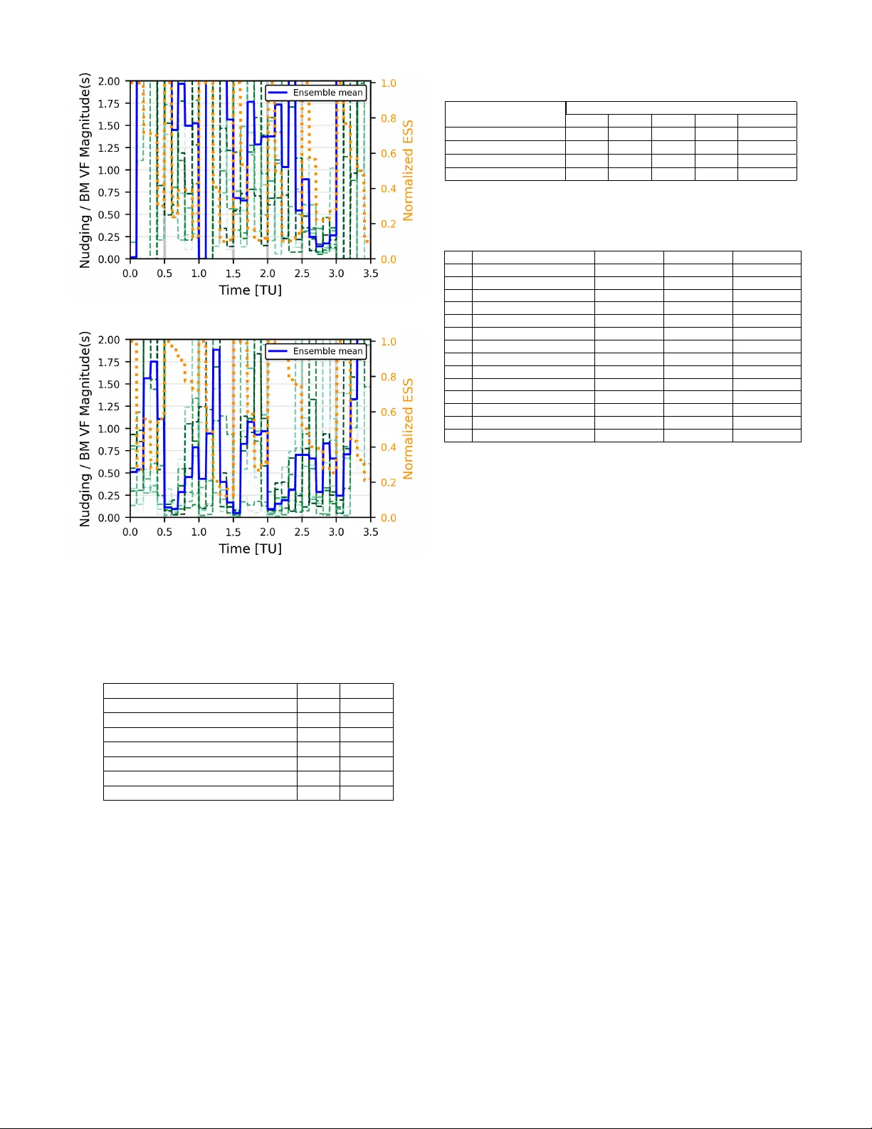
A V ariational Pseudo-Observ ation Guided Nudged P article Filter Theofania Karampela and Ryne Beeson Mechanical and Aer ospace Engineering Princeton University Princeton, New Jersey , USA tk4161@princeton.edu and ryne@princeton.edu Abstract —Nonlinear filtering with standard Particle Filter (PF) methods requir es mitigative techniques to quell weight degeneracy , such as resampling. This is especially true in high- dimensional systems with sparse observations. Unfortunately , such techniques are also fragile when applied to systems with exceedingly rare e vents. Nonlinear systems with these pr operties can be assimilated effectively with a control-based PF method known as the Nudged Particle Filter (nPF), but this method has a high computational cost burden. In this work, we aim to retain this strength of the nudged method while reducing the computational cost by introducing a variational method into the algorithm that acts as a continuous pseudo-observation path. By maintaining a PF repr esentation, the resulting algorithm con- tinues to capture an approximation of the filtering distribution, while reducing computational runtime and improving r obustness to the “rare” event of switching phases. Preliminary testing of the new approach is demonstrated on a stochastic variant of the nonlinear and chaotic Lorenz 1963 (L63) model, which is used as a surrogate for mimicking “rare” events. The new approach helps to overcome difficulties in applying the nPF for realistic problems and performs fav orably with respect to a standard PF with a higher number of particles. Index T erms —Particle Filter , Nudged Particle Filter , V ari- ational Method, V ariational Nudged Particle Filter , Optimal Importance Sampling, Lorenz 1963, Rare Events I . I N T R O D U CT I O N In this manuscript we are interested in the filtering solution to partially observ able continuous-time signal processes ( X t ) with discrete-time observ ations ( Y t k ) dX t = f ( X t ) dt + σ ( X t ) dW t , X 0 = x ∈ R m , Y t k = h ( X t k ) + ξ t k , Y 0 = 0 ∈ R d , (1) where ( t k ) is an increasing sequence of observation times index ed by k ∈ N with t 0 = 0 , and ξ t k ∼ N (0 , Σ y ) is the observation noise that is independent of the standard Brownian motion (BM) W t that drives the signal process X t . W e denote the filtering solution of X at time t giv en the observations up to time t k ≤ t by p t ( x |F Y k ) . W e use F Y k to denote all observations up to time t k (simplifying the subscript from t k to just k for bre vity here and in what follows) and hence the prior conditional distribution at time t k is p k ( x |F Y k − 1 ) and the posterior is p k ( x |F Y k ) . Additional properties that we assume of ( 1 ), and that driv e choices in filtering algorithms and the method dev eloped in this work, is that X represents a state of very high dimension Fig. 1: L63 deterministic attractor with initial conditions (see T able III ) used in numerical experiments (see § IV ). (e.g., in the extreme cases of geophysical data assimilation [ 1 ], [ 2 ], this can be m ∼ O (10 8 ) degrees of freedom that results from the discretization of partial differential equations (PDEs) describing physical processes), that the prior and posterior distributions are non-Gaussian, that the numerical solution of the signal process giv en in ( 1 ) is computationally demanding, and lastly , that intermittent aperiodic behavior characteristic of rare ev ents takes place. A rare event is one that is represented by a low probability of occurrence; often associated with a state X in the tail of the distribution p ( x |F Y ) . Geophysical models generally possess the first three properties [ 1 ], [ 3 ], and examples of rare e vents include hurricanes, earthquakes, and rapid ov erturning in ocean flows [ 4 ], [ 5 ], [ 6 ]. Filtering prob- lems with these characteristics lead naturally to methods of either a variational or a low-sample ensemble-based approach. V ariational methods provide a smoothing solution for the maximum a posteriori (MAP) state [ 3 ], [ 7 ], [ 8 ]. Their dis- advantage is that they only provide a MAP state and not a representation of the full distribution or ev en higher-order moments. Lastly , because of the computational dif ficulty of solving such problems for high-dimensional systems, param- eters that should be state and time varying are often fixed to 1 static background (or climatological) values and hence do not represent the true near term v ariability . An alternativ e solution is to approximate the filtering distribution with an importance sampling approach. W ith (( X i , w i ) ∼ p ) N i =1 representing N ∈ N pairs of samples ( X i ) with normalized weights ( w i ) from a distribution p , the N - ensemble approximation p N to p is p N ( dx ) ≡ N X i =1 w i δ X i ( dx ) ≈ p ( dx ) , (2) where δ X i is the Dirac distribution at X i . The class of PF methods allo w the weights to change during assimilation cycles; a reflection of the f act that the y are importance weights. In the standard approach, the particle locations remain fixed during the Bayesian update. As we will recall in § II , the adjustment of the particle weights at times of filtering updates is what ultimately leads to the well known issue of particle degenerac y . Some recent ef forts in the literature navig ate the issue of particle degeneracy by maintaining equal weights during Bayes’ update by reframing the discrete-time update as a flo wing of the particles in the state-space during a pseudo-observation interval [ 9 ], [ 10 ], [ 11 ], solving for an equiv alent flow map [ 12 ], [ 13 ], or an implicit mapping [ 14 ]. Additionally , comments on how the flow-based approaches distinguish themselves from the main method of this paper , based on the nPF, will be giv en in § II . There are filtering methods that are ensemble-based, where the weights are chosen as equal (i.e., w i = 1 / N ) and remain equal throughout the filtering update. Common families of these methods include the well-known variants of the En- semble Kalman Filter (EnKF) [ 15 ], [ 16 ], Unscented Kalman Filter (UKF) [ 17 ], and Gaussian Mixture Model (GMM) [ 18 ]. Although these methods provide a built-in protection from particle degenerac y , just as the flow-based and flow-map PF methods do, these approaches do not provide the flexibility to account for modified particle dynamics between observations which would be reflected in v arying importance weights; this is an essential characteristic of the nPF and provides greater ability to adapt to problems with nonlinear dynamics or “rare” ev ents. When N ≪ m , the distribution p N is unlikely to have state representations in the tails of p , and therefore methods that generate the prior distribution by advecting each particle under the dynamics gi ven by ( 1 ) are likely to result in a prior that does not have support containing the true state in the case of a “rare” event. If instead the particles are allowed to adjust their paths to reflect the most likely path between observations; for instance, by introducing a control u t to the dynamics dX t = f ( X t ) dt + u t dt + σ ( X t ) dW t , (3) then the posterior distribution at one time can be effecti vely steered to a representative prior distribution even in the pres- ence of these “rare” events. The approach of ( 3 ) is the approach for the nPF [ 19 ], [ 20 ] that this work builds upon and will be recalled in § II . The nPF was originally proposed for mitigating weight degenerac y of the standard PF in nonlinear chaotic and sparse filtering problems, but also has the required formulation to address the “rare” e vent problem. The central drawback of the nPF is that the exact control solution, which is continuous in time, is often approximated by Monte Carlo (MC) approaches that con verge slowly , and hence it is computationally burdensome. The aim of this manuscript is to test the efficac y of using a hybrid V ariational nudged Particle Filter (V ar -nPF) approach, whereby the v ariational method is used to generate a pseudo- observation path that provides state-space guidance of the nPF particles. As will become clear in the explanations contained in § III , this allo ws for a shorter time horizon optimal control problem to be solved for the nPF and hence provides an a venue to reduce its computational cost, while still maintaining the ability to approximate the filtering distribution at all times and handle the case of “rare” e vents. The paper now proceeds as follows. In § II we recall the basics of the standard bootstrap PF and provide background on the nPF. W e provide relev ant citations to the literature in this section for those methods and set notation. In § III we detail the variational approach used in this work and the new method that combines it with the nPF. In § IV we provide the model setup for a stochastic L63 system, shown in Fig. 1 , that will serve as a surrogate to mimick “rare” e vents in geophysical problems. Simulation results are also giv en and discussed in this section. Final remarks and future efforts are giv en in § V . I I . S TA N DA R D A N D N U D G E D P A RT I C L E F I LT E R A. Standard P article F ilter The standard (bootstrap) PF [ 21 ], with resampling proceeds in three distinct steps (prior , Bayes’ update, and resampling) that repeat for each observation cycle. W e assume that we start with an N -particle approximation of the posterior distribution at time t k − 1 with normalized weights P N i =1 w i = 1 , as ex- pressed in ( 2 ). The standard PF with resampling then proceeds recursiv ely by generating the prior at time t k by adv ecting each particle X i k − 1 under the dynamics giv en in ( 1 ) to time t k p N k ( dx |F Y k − 1 ) = N X i =1 w i k − 1 δ X i k ( dx ) . (4) Then, given the observation Y k , unnormalized weights are calculated according to Bayes’ formula e w i k = w i k − 1 p k ( Y k | X i k ) , (5) where p k ( Y k | X i k ) is the lik elihood function associated with the measurement process gi ven in ( 1 ). After normalizing these weights w i k = e w i k / P N i =1 e w i k , the posterior distribution at time t k is as p N k ( dx |F Y k ) ≡ N X i =1 w i k δ X i k ( dx ) . (6) Lastly , if the particle weights are degenerate (i.e., the variance of the weights is large), then the particles are independently 2 and identically resampled from the particle set ( X i k ) with probability according to the normalized weights ( w i k ) . This process results in particles that may have the same support locations, but now with equal weights (i.e., w i k = 1 / N ). T o determine whether the particle approximation is degen- erate in this work, we use an approximation of the Effectiv e Sample Size (ESS) [ 22 ], [ 23 ]. With the vector of normalized weights denoted as w , the approximation is giv en by N eff ≡ 1 / ⟨ w , w ⟩ . W e use the threshold of N eff < N / 2 to trigger resampling with the universal (or systematic) resampling approach [ 24 ]. B. Nudged P article F ilter The key difference between the nPF and a standard PF algorithm is that the particles are advected under the dynamics giv en by ( 3 ) as opposed to ( 1 ). The forcing u t is a nonlinear control law that is obtained independently for each particle X i by solving a finite-time horizon optimal control problem (OCP) that is dependent on the new observ ation. The result of applying the control is that particles are nudged toward the area of high likelihood for the new observation. The setup and main result of this OCP are given in the following theorem statement. Notation: The superscript notation X k,x for any par- ticle indicates an initial condition at x ∈ R m at time t k . C ([ t k , t k +1 ]) is the space of continuous functions and a superscript asterisk (e.g., σ ∗ ) indicates the transpose of a matrix. Theorem II.1 (Nudged Particle Filter (nPF) [ 19 ], [ 20 ]) Given a sample X k,x t k ∼ p N k ( dx |F Y k ) and observation Y k +1 , the solution of the OCP min u ∈ C ([ t k ,t k +1 ]) { J ( u ; k , x, Y k +1 ) ≡ E  Z t k +1 t k 1 2 ⟨ u s , R − 1 s u s ⟩ ds + g ( X k,x k +1 , Y k +1 )  , (7) with dynamic constraint for X k,x t , t ∈ [ t k , t k +1 ) given by ( 3 ) , g the log-likelihood of the observation, R s the diffusion matrix of the stochastic forcing in ( 3 ) , is (under r easonable assumptions) a feedbac k contr ol law u ( t, x ) = 1 Φ( t, x ) R t ∇ x Φ( t, x ) , (8) with Φ and ∇ x Φ solutions to linear parabolic PDEs that can be written in terms of F e ynman-Kac r elations Φ( t, x ) = E h exp( − g ( η k,x k +1 , Y k +1 )) i , (9) and ∇ x Φ( t, x ) = − E h exp( − g ( η k,x k +1 , Y k +1 )) exp  Z t k +1 t k ∇ x f ( η k,x s ) ds  ∇ x g ( η k,x k +1 , Y k +1 )  , (10) with η k,x k +1 being realizations of ( 1 ) . An important result of the control solution given in ( 8 ) is that particles attempt to stay faithful to the modeled dynamics of ( 1 ). Any de viation is accounted for by a change in their unnormalized weights. Corollary II.1 (nPF Radon-Nikodym Deriv ativ e [ 20 ]) The unnormalized weights of the sample X k,x t under the contr ol law ( 8 ) given by Theor em II.1 change accor ding to the continuous-time Radon-Nikodym derivative dµ i d b µ i     t ∈ [ t k ,t k +1 ] = exp  − Z t t k ⟨ v ( s, X i s ) , dW s ⟩ − 1 2 Z t t k ⟨ v ( s, X i s ) , v ( s, X i s ) ⟩ ds  , (11) wher e v ( s, X i s ) = σ ∗ ∇ x  log Φ( s, X i s )  when R ≡ σ σ ∗ . Ther efore, in contrast to ( 5 ) , the unnormalized weights of the nPF are e w i k +1 = dµ i d b µ i     t k +1 w i k p k ( Y k +1 | X i k +1 ) . (12) For additional details on the nPF, more advanced versions, and its application to higher-dimensional mathematical models than giv en in this manuscript, we direct the reader to some of the recent literature [ 25 ], [ 26 ], [ 27 ]. 1) Adaptive Nudging Calculation: Numerical implementa- tion of the nPF requires an approximation of ( 9 ) and ( 10 ), which is most directly accomplished via MC. T o ensure that our approximation of the expectations and hence the control solution has con verged to an acceptable tolerance le vel, an adaptiv e scheme is used whereby we calculate the control for an increasing number of realizations ( η k,x k +1 ) . This is implemented in batch form to improve efficiency and reuse previously computed realizations. In particular , let K ∈ N be a batch size and j ∈ N the j -th iteration of the algorithm to compute the control approximation u j K t , with j K total realizations. Additionally , let ˆ u j K t ≡ u j K t / | E [ f ( X t )] | (13) be the normalized control magnitude. Repeating this approxi- mation for the ( j + 1) -th iteration, we define the normalized control variation to be δ ˆ u j +1 t ≡ | ˆ u ( j +1) K t − ˆ u j K t | . (14) Then for a user specified tolerance ϵ u > 0 , if δ ˆ u j +1 ≤ ϵ u , the approximate control solution ˆ u ( j +1) K t is said to have con verged, and otherwise we proceed to the ( j + 2) -th iteration of the algorithm. 2) Additional Remarks: W e finish this section by making clear the distinction between the nPF and flo w-based PF algorithms mentioned in § I , and in particular those deriv ed also from a control perspectiv e such as the feedback parti- cle filter (FPF) [ 11 ]. The main distinction is that the FPF applies a control law in the pseudo-observ ation interval for the Bayes’ update, whereas the nPF applies a control to the particles between observations. Since the control in the nPF 3 Fig. 2: Schematic ev olution of a single particle within one observation interv al for the nPF (left) and the V ar -nPF (right). occurs between observations, the weights must be changed accordingly . Another approach that is closely related to the nPF, but motiv ated by large deviation theory and derived from a varia- tional method approach, has been applied to a model for the rare event of the Kuroshio current [ 28 ]. I I I . V A R I A T I O N A L N U D G E D P A RT I C L E F I L T E R It is not practical to solve for a continuous-time control of the nPF at every time t ∈ [ t k , t k +1 ) between observ ations. Therefore, the standard implementation is to partition the in- terval between observations into M ∈ N equal-length control subintervals with a collection of endpoints defining them given by the indexed set ( t k ( j ) ) M j =0 . Then a control solution is found for the time t k ( j ) at the beginning of each subinterval, by solving the nonlinear OCP in ( 7 ) from t k ( j ) to t k +1 , and this control is then held constant in application for the remainder of the subinterval [ t k ( j ) , t k ( j +1) ) . As the expectations in ( 9 ) and ( 10 ) are over the state η k,x k +1 at the final time, the earlier control subintervals are computationally more expensi ve (i.e., longer numerical integration times) than the later ones; this is shown in Fig. 2 (left). Additionally , the earlier subintervals are more sensitiv e to the nonlinear dynamics and noise perturbations, which requires larger batch sizes in the adaptiv e nudging calculation described in § II-B1 . The central contribution of this paper is to introduce a pseudo-observation path that enables a fixed computational cost for the nudging control in ev ery subinterv al. This pseudo- observational path also appears to help moderate the weight variance due to the Radon-Nikodym deriv ative for the nPF as giv en in Corollary II.1 . For clarity of discussion, let us fix a single observation interval [ t k , t k +1 ) with observation Y k +1 and particles ( X i k ) (refer to Fig. 2 (right)). W e then aim to find the most likely path of the observation; that is a path ( Y † t ) t ∈ [ t k ,t k +1 ] such that Y † t k +1 ≈ Y k +1 . This likely observation path can then be substituted into ( 9 ) and ( 10 ) so that control solutions at each subinterval can be calculated with realizations ending at the end of the subinterv al, t k ( j +1) , instead of the full observation interval, t k +1 . T o find such a likely observation path, we instead solve for a state-space path ( X † t ) that is the most likely path from a giv en initial condition to a state that generates the observation Y k +1 . In particular , this state-space path is found by solving a variational problem. Specifically , what is often referred to as the strong constraint 4- dimensional variational (sc4D V ar) approach in the geophysical data assimilation community [ 3 ], [ 7 ], [ 8 ]. The optimization problem to be solved is min x ∈ R m  J ( x ; k , Y k +1 ) ≡ 1 2 ⟨ ∆ x,  Σ N k  − 1 ∆ x ⟩ + 1 2 ⟨ ∆ y , Σ − 1 y ∆ y ⟩  , (15) with µ N k and Σ N k an empirical mean and covariance respec- tiv ely (e.g., for the nPF solution) at time t k , ∆ x ≡ x − µ N k , ∆ y ≡ Y k +1 − h ( X k,x k +1 ) is the innovation, where X k,x k +1 is the solution of the deterministic dynamics (i.e., σ = 0 in ( 1 )). If ( X † t ) is no w the most likely path integrated under the deterministic dynamics, starting from an optimal solution to ( 15 ), then the pseudo-observation path is simply Y † t ≡ h ( X † t ) . In the case where the measurement operator is simply the identity mapping (i.e., h is the identity matrix Id . ∈ R m × m ), then the observation and state-space are identical, and we can use X † t as the pseudo-observ ation path itself. W e note that it is natural to also extend ( 15 ) to the case of multiple 4 observation at dif ferent times, but in this work we only consider assimilation cycles with one observation time. A. The V ariational Nudged P article F ilter Algorithm The combination of the variational approach with the nPF now proceeds by first computing a solution to the v ariational problem of ( 15 ) for a gi ven control subinterv al described in § III . Advecting the a deterministic state starting from this optimal initial condition to the end of the control subinterv al generates a target pseudo-observ ation Y † t k ( j +1) that is then used as a conditional parameter (pseudo-observation) to the nPF OCP in Theorem II.1 . These pseudo-observations are shown in Fig. 2 (right). As discussed at the beginning of this section, the nudged control problem is now always of fixed time duration, being equal to the subinterv al length t k ( j ) − t k ( j +1) . W e repeat this procedure for each control subinterval, including the final one, where we still use the produced pseudo-observation Y † t k +1 instead of the true gi ven one Y k +1 . This ne w algorithm is labeled V ar-nPF throughout the remainder of the paper . For the numerical experiments giv en in § IV , the optimiza- tion of the variational problem gi ven by ( 15 ) is solved with a bounded limited Broyden-Fletcher -Goldfarb-Shannon (L- BFGS-B) [ 29 ]. In the case that Σ N k is poorly conditioned, we add a small regularization term ϵ Id . , with 0 < ϵ ≪ 1 . I V . N U M E R I C A L E X P E R I M E N T S In this section we first explain the setup of a stochastic version of the L63 model [ 30 ] to be used in experiments, then pertinent simulation parameters, and lastly the findings and comparisons of indi vidual and MC experiments. A. The Stoc hastic Lorenz 1963 Model The deterministic definition of the L63 model [ 30 ] has a drift vector field f for ( 1 ) gi ven by f : ( x, y , z ) 7→ ( α ( y − x ) , γ x − y − xz , xy − β z ) , (16) where standard parameters are α = 10 , γ = 28 , β = 8 / 3 , and are used in this work. With these parameters the L63 model is chaotic and solutions conv erge onto an attractor as sho wn in Fig. 1 . The error doubling time, an indicator of how chaotic a system is, is approximately 0.76 time units (TU), and the av erage time that a solution switches from one lobe of the attractor to the other is approximately 1.75 TU. The nPF requires a stochastic dynamical system for its application. W e therefore modify the L63 model by adding the stochastic forcing shown in ( 1 ). In particular , we consider the additiv e noise case, where the dispersion coefficient σ is constant and defined so that the diffusion coefficient for the stochastic forcing is σ σ ∗ ≡   2 1 0 . 5 1 2 1 0 . 5 1 2   . (17) B. Simulation P arameters All simulations will use N = 10 particles, observation step-size ∆ t obs = 0 . 5 TU, and final time t f = 3 . 5 TU. Numerical intergration is with a W iener-RK4-Maruyama scheme, with integrator step-size ∆ t = 0 . 01 TU. Unless stated otherwise, the initial condition is chosen as x = (1 . 508870 , − 1 . 531271 , 25 . 46091) , which is identified in Fig. 1 by the red star . The initial particle ensembles for any PF method is via sampling from a Gaussian N ( µ, 2 Id . ) , where µ represents one of the initial conditions shown in T able III and labeled on the attractor in Fig. 1 . These representati ve initial conditions were generated from a long deterministic trajectory of the attractor with the aim to provide low-discrepanc y samples of the attractor itself. These initial conditions therefore provide dynamically distinct states and promote MC results that pro- vide a fairer benchmarking of the various filtering methods. The observation operator is h = Id . with noise cov ariance Σ y = 2 Id . , so that the standard deviation of the observation noise is less than 5% of the characteristic range of the L63 state variables. This ensures that the observations are informative without dominating the model dynamics. Each observation interval is partitioned into M = 5 control subintervals. In the solution of the OCP for each subinterv al, we use K = 2 trajectory realizations per batch together with the adaptiv e nudging strategy described in § II-B1 . A tolerance of ϵ u = 0 . 1 is used for the adaptive nudging calculation. A maximum of 50 batches (i.e., 100 total realizations) is allowed in the calculation, though none of the experiments required this many to conv erge to our tolerance of ϵ u . C. Simulation Results W e first consider a fixed simulation scenario to illustrate the prototypical behavior of the PF, nPF, and V ar-nPF methods. Then ha ving established and visualized the beha vior of these methods, we perform a MC analysis. Pr ototypical Behavior: T o better understand and visualize particle motion within a single observation interv al across the three PF variants presented in this work, we consider the case where all filters use the same samples generated from a Gaussian distribution with mean giv en by the red star in Fig. 1 . These samples are shown by gray circle markers in Fig. 3 , where they have been projected onto the dominate subspace spanned by the prior states of all the particles (i.e., all the methods) at the first observation time. This subspace is found by a singular value decomposition of a matrix with all the particle states as columns. All three methods perform filtering with the same true hidden signal ( black line) and observations ( green markers) as shown in Fig. 4 . Fig. 3 shows the prior particle locations with triangular markers, and the size of the mark ers is a reflection of each particles normalized weight. In particular , the PF does not change the weights of the particles, whereas the nPF and V ar- nPF weights do change as the particles attempt to nudge closer to the observation. The PF normalized ESS (nESS) changes from 1 for the prior to 0.15 after the Bayes’ update, where as 5 Fig. 3: Initial particle samples for all methods shown with gray circle markers . Prior states of each method (triangles) at the first observation t = 0 . 5 scaled to the normalized weight. the nPF goes from 0.3 to 0.1, and the V ar -nPF from 0.56 to 0.41. While the PF spreads significantly after advection, the nPF, and especially those of the V ar -nPF, mo ve toward the observation. This observation interval corresponds to a “rare” ev ent (i.e., a transition of the lobes), as sho wn in Fig. 4 . It is for this reason that the PF, which has no control, ends up with too much variance at the time of the observation. It is promising that all of the V ar-nPF particles arrive in the area of high likelihood for the observation, and most with reasonably good weights. W e see this behavior also holds true for other switching times between lobes in Fig. 4 . The nPF particles that do not arriv e near the observ ation is due to our implementation that prevents nudging to occur if it would reduce an individual particles unnormalized weight too much. W e refer to such cases in this paper as a “zero control rollback” (i.e., we calculate the proposed control, but ultimately do not apply it–see T able I ). It is interesting to compare the nudging control magnitude relativ e to the BM vector field (VF) as shown in Fig. 5 for this experiment. This relative nudging to BM VF is shown in green for each particle and the ensemble mean in blue . The nESS is sho wn with the second y-axis in orange . Of particular note is the aggressiv e control of the nPF, whereas our new method is able to relax the proposed relativ e control and hence deli ver more particles to the observation location and with better nESS. This is most easily observed from the ensemble mean of the nudging relative to the BM VF taking larger values (above the upper bound of the plot) for the nPF, but only at the end of the simulation for the V ar- nPF. These occurrences correspond to larger dispersion in the particles at those times, which can be seen in Fig. 4 . It is important to note that the nudging to BM VF ratio should re- main below a value of one on average if we are to believ e that the stochastic model is properly defined (i.e., if the stochastic forcing represents model uncertainty , then it is parameterized properly to reflect reality and our filtering method is not trying (a) PF (b) nPF (c) V ar-nPF Fig. 4: T ime e volution of the first state component (i.e., x ). to overpo wer the model defined dynamics). W e indeed see this to happen more often in the ne w V ar-nPF, which is a promising indicator . The computational ov erhead introduced by the v ariational component was also analyzed for this experiment and MC runs, which sho wed similar trends. In particular , solving the variational problem accounts for approximately 40.5% of the 6 (a) nPF (b) V ar-nPF Fig. 5: Nudging magnitude relati ve to BM forcing ( green ), ensemble mean for this relati ve control ( blue ), and the nESS. T ABLE I: Comparison between PF, nPF, and V ar-nPF for one experiment with the red star initial mean condition. Metric nPF V ar -nPF Mean of Control Magnitude ∥ u ∥ 2 18.14 4.55 Maximum of Control Magnitude ∥ u ∥ 2 220.91 41.13 Fraction of Zero Control Rollback 0.166 0.000 A verage Nudging / BM VF ratio 2.87 0.77 Maximum Nudging / BM VF ratio 60.62 9.69 A verage RMSE 4.92 1.48 Runtime (s) 13.49 7.8 total V ar-nPF runtime. The remaining run time was due to the nPF control calculations. Although the variational component constitutes a significant portion of the computation, it does not dominate the ov erall runtime and reduces the computational cost compared to the nPF for this experiment (see T able I ). As long as a decent optimization solution is provided by the variational part of the new method, it has the potential to scale much better for higher dimensional and longer observation interval problems. The av erage Root Mean Square Error (RMSE) for each method sho wn in T able I , is the av erage ov er the state and time with respect to the true signal. T ABLE II: 100 MC runs; ted star initial mean in Fig. 1 Metric Filter T ype PF 10 PF 30 PF 40 nPF V ar-nPF Number of Particles 10 30 40 10 10 A vg. RMSE 6.35 4.47 3.66 6.39 2.91 Normalized A vg. ESS 0.27 0.26 0.27 0.17 0.26 Runtime (s) 18.47 30.45 37.21 283.9 132.92 T ABLE III: MC (1000 total runs, 100 for each µ initial condition), reporting A vg. nESS, A vg. RMSE, and runtime. # µ Initial Condition PF nPF V ar -nPF nESS RMSE nESS RMSE nESS RMSE * (1 . 509 , − 1 . 531 , 25 . 461) 0.27 6.35 0.17 6.39 0.26 2.91 1 ( − 3 . 622 , 2 . 487 , 29 . 784) 0.26 6.64 0.14 8.34 0.25 4.37 2 ( − 8 . 587 , − 14 . 288 , 16 . 895) 0.30 6.83 0.20 6.43 0.27 4.64 3 ( − 14 . 411 , − 8 . 058 , 40 . 440) 0.26 6.50 0.17 5.79 0.24 4.45 4 (14 . 418 , 11 . 236 , 37 . 915) 0.25 7.96 0.18 5.69 0.24 6.17 5 (4 . 133 , 6 . 815 , 14 . 316) 0.28 8.02 0.19 7.75 0.26 5.35 6 ( − 2 . 895 , − 5 . 123 , 11 . 843) 0.32 5.57 0.19 5.47 0.27 3.98 7 ( − 5 . 802 , − 7 . 589 , 20 . 507) 0.36 4.00 0.22 3.70 0.31 2.94 8 (10 . 347 , 17 . 701 , 17 . 250) 0.25 8.86 0.16 7.42 0.24 5.41 9 (3 . 072 , − 0 . 052 , 26 . 056) 0.25 7.96 0.14 8.80 0.25 4.28 10 (1 . 909 , − 0 . 842 , 24 . 846) 0.22 10.31 0.17 6.76 0.26 2.98 A vg. — 0.28 7.27 0.18 6.62 0.26 4.46 A vg. Computational Runtime 23.39 202.08 129.87 Monte Carlo Simulations: T o validate that the trends and observations seen in the single e xperiment described in the last section hold in general, we performed a MC analysis of 100 simulations with the red star initial condition (see Fig. 1 ) as the mean of a Gaussian to be sampled. These MC results are gi ven in T able II and it shows that the nPF improves the av erage RMSE slightly over the PF, but with degradation in the nESS. The limiting factor in the performance of the nPF to achiev e better RMSE is due to the fact that we only use M = 5 control subinterv als, which therefore results in the non- insignificant fraction of zero control rollbacks detailed in T able I . Using more control subinterv als would drastically increase the runtime of the nPF, which was already deemed high for comparisons to the PF for this low-dimensional model. There is noticable improvement in the the RMSE for the new V ar-nPF without a degradation in the nESS. T able I also shows MC results for the PF with an increasing number of particles, so that a better comparison of the performance of the methods on an estimation accuracy and computational runtime lev el can be made. Although the V ar-nPF achie ves the best av erage RMSE it is lik ely still computationally more e xpensiv e for a PF method with a suf ficiently high number of particles (e.g., it seems that 50 to 60 particles may suf fice to achiev e the same RMSE but with half the run time). W e hypothesis that the estimation accuracy and computational runtime will be more fav orable for the ne w method in future testing of higher dimensional models. T o further validate that the trends and observ ations hold generally for the application of the methods to the stochastic L63 model, we perform another MC simulation, but with 100 runs for each of the 10 initial means giv en in T able III and labeled in Fig. 1 . The PF exhibits a consistently low 7 nESS and relativ ely large RMSE, indicating significant weight degenerac y . The nPF improves the estimation accuracy in sev eral cases, but does not reduce the estimation error across all initial conditions. Notably , the new V ar -nPF approach achiev es consistently lower RMSE, demonstrating improv ed robustness with respect to variations in the initial state of the L63. These results indicate that incorporating the modified variational approach enhances the accuracy of the filtering process. The computational runtime trends from T able II are maintained in this MC experiment, as sho wn by the last row of T able III . V . C O N C L U S I O N S In this paper , we hav e introduced a variational pseudo- observation guided nPF for filtering nonlinear chaotic systems with sparse observations that may exhibit “rare” ev ents. By generating intermediate pseudo-observations within each ob- servation interval, the proposed approach replaces long time- horizon OCPs with shorter ones. Numerical results on the stochastic L63 show that the V ar-nPF improves estimation accuracy relativ e to both PF and nPF while reducing compu- tational cost. This provides gentler nudging of the particles in each subinterval, enabling more consistent control and promoting better weight div ersity . The observation interval used in this work was shorter than the average switching time between lobes of the L63 attractor . T o better mimic a “rare” e vent, future work will test on longer duration regimes that are more comparable to the switching timescale. This setting will better test the sensiti vity of the variational component of the V ar -nPF. Future efforts will also in vestigate the use of regularized variational methods [ 31 ], as well as test the V ar-nPF on higher- dimensional systems such as the Lorenz 1996 model [ 32 ] and geophysical models demonstrating observed rare events [ 6 ]. R E F E R E N C E S [1] P . J. van Leeuwen, H. R. K ¨ unsch, L. Nerger , R. Potthast, and S. Reich, “Particle filters for high-dimensional geoscience applications: A review , ” Quarterly Journal of the Royal Meteor ological Society , vol. 145, no. 723, pp. 2335–2365, 2019. [Online]. A v ailable: https://rmets.onlinelibrary .wiley .com/doi/abs/10.1002/qj.3551 [2] C. Snyder, T . Bengtsson, P . Bickel, and J. L. Anderson, “Obstacles to high-dimensional particle filtering, ” Monthly W eather Review , vol. 136, no. 12, pp. 4629–4640, 2008. [3] G. Evensen, F . C. V ossepoel, and P . J. van Leeuwen, Data Assimilation Fundamentals: A Unified F ormulation of the State and P arameter Estimation Pr oblem . Springer International Publishing, 2022. [Online]. A vailable: https://doi.org/10.1007/978- 3- 030- 96709- 3 [4] J. A. Bucklew , Introduction to Rare Event Simulation . Ne w Y ork, NY : Springer New Y ork, 2004. [Online]. A vailable: https: //doi.org/10.1007/978- 1- 4757- 4078- 3 [5] E. V anden-Eijnden and J. W eare, “Rare ev ent simulation of small noise dif fusions, ” Communications on Pure and Applied Mathematics , vol. 65, no. 12, pp. 1770–1803, 2012. [Online]. A vailable: https://onlinelibrary .wiley .com/doi/abs/10.1002/cpa.21428 [6] B. Qiu and W . Miao, “Kuroshio path variations south of japan: Bimodality as a self-sustained internal oscillation, ” Journal of Physical Oceanography , vol. 30, no. 8, pp. 2124 – 2137, 2000. [Online]. A vailable: https://journals.ametsoc.org/view/journals/phoc/30/ 8/1520- 0485 2000 030 2124 kpvsoj 2.0.co 2.xml [7] O. T alagrand and P . Courtier, “V ariational assimilation of meteorological observations with the adjoint v orticity equation. i: Theory , ” Quarterly Journal of the Royal Meteor ological Society , vol. 113, no. 478, pp. 1311–1328, 1987. [Online]. A vailable: https://rmets.onlinelibrary .wiley . com/doi/abs/10.1002/qj.49711347812 [8] P . Courtier and O. T alagrand, “V ariational assimilation of meteorological observations with the adjoint vorticity equation. ii: Numerical results, ” Quarterly Journal of the Royal Meteor ological Society , vol. 113, no. 478, pp. 1329–1347, 1987. [Online]. A vailable: https://rmets.onlinelibrary .wiley .com/doi/abs/10.1002/qj.49711347813 [9] F . Daum and J. Huang, “Nonlinear filters with log-homotopy, ” in Signal and Data Pr ocessing of Small T argets 2007 , O. E. Drummond and R. D. T eichgraeber, Eds., vol. 6699, International Society for Optics and Photonics. SPIE, 2007, p. 669918. [Online]. A vailable: https://doi.org/10.1117/12.725684 [10] U. D. Hanebeck, K. Briechle, and A. Rauh, “Progressiv e Bayes: a new framew ork for nonlinear state estimation, ” in Multisensor , Multisource Information Fusion: Ar chitectur es, Algorithms, and Applications 2003 , B. V . Dasarathy , Ed., vol. 5099, International Society for Optics and Photonics. SPIE, 2003, pp. 256 – 267. [Online]. A vailable: https://doi.org/10.1117/12.487806 [11] T . Y ang, P . G. Mehta, and S. P . Meyn, “Feedback particle filter , ” IEEE T ransactions on Automatic Contr ol , vol. 58, no. 10, pp. 2465–2480, 2013. [12] A. Spantini, R. Baptista, and Y . Marzouk, “Coupling techniques for nonlinear ensemble filtering, ” SIAM Review , vol. 64, no. 4, pp. 921–953, 2022. [Online]. A vailable: https://doi.org/10.1137/20M1312204 [13] S. Reich, “Data assimilation: The schr ¨ odinger perspecti ve, ” Acta Nu- merica , vol. 28, pp. 635–711, 2019. [14] A. J. Chorin and X. Tu, “Implicit sampling for particle filters, ” Pr oceedings of the National Academy of Sciences , vol. 106, no. 41, pp. 17 249–17 254, 2009. [Online]. A vailable: https://www .pnas.org/doi/ abs/10.1073/pnas.0909196106 [15] G. Evensen, “Sequential data assimilation with a nonlinear quasi- geostrophic model using monte carlo methods to forecast error statistics, ” Journal of Geophysical Resear ch: Oceans , vol. 99, no. C5, pp. 10 143–10 162, 1994. [Online]. A vailable: https://agupubs. onlinelibrary .wiley .com/doi/abs/10.1029/94JC00572 [16] G. Burgers, P . J. van Leeuwen, and G. Evensen, “ Analysis scheme in the ensemble kalman filter , ” Monthly W eather Review , vol. 126, no. 6, pp. 1719 – 1724, 1998. [Online]. A vailable: https://journals.ametsoc.org/vie w/journals/mwre/ 126/6/1520- 0493 1998 126 1719 asitek 2.0.co 2.xml [17] S. Julier and J. Uhlmann, “Unscented filtering and nonlinear estimation, ” Pr oceedings of the IEEE , vol. 92, no. 3, pp. 401–422, 2004. [18] H. Sorenson and D. Alspach, “Recursive bayesian estimation using gaussian sums, ” Automatica , vol. 7, no. 4, pp. 465–479, 1971. [Online]. A vailable: https://www .sciencedirect.com/science/article/pii/ 0005109871900975 [19] N. Lingala, N. Perkowski, H. C. Y eong, N. S. Namachchivaya, and Z. Rapti, “Optimal nudging in particle filters, ” Probabilistic Engineering Mechanics , vol. 37, pp. 160–169, July 2014. [Online]. A vailable: https://doi.org/10.1016/j.probengmech.2013.08.007 [20] H. C. Y eong, R. T . Beeson, N. S. Namachchiv aya, and N. Perkowski, “Particle filters with nudging in multiscale chaotic systems: W ith ap- plication to the lorenz ’96 atmospheric model, ” Journal of Nonlinear Science , vol. 30, no. 4, pp. 1519–1552, 2020. [21] N. J. Gordon, D. J. Salmond, and A. F . M. Smith, “Novel approach to nonlinear/non-Gaussian Bayesian state estimation, ” IEE Pr oceedings F - Radar and Signal Processing , vol. 140, no. 2, pp. 107–113, 1993. [22] N. Bergman, “Recursive bayesian estimation: Navigation and tracking applications, ” Ph.D. dissertation, Link ¨ oping University , Link ¨ oping, Sweden, 1999. [Online]. A vailable: https://www .rt.isy .liu.se/research/ reports/Ph.D.Thesis/PhD579.pdf [23] J. S. Liu and R. Chen, “Sequential monte carlo methods for dynamical systems, ” Journal of the American Statistical Association , vol. 93, no. 433, pp. 1032–1044, 1998. [Online]. A vailable: http://www .jstor .org/stable/2669847 [24] G. Kitagawa, “Monte carlo filter and smoother for non-gaussian nonlinear state space models, ” Journal of Computational and Graphical Statistics , vol. 5, no. 1, pp. 1–25, 1996. [Online]. A vailable: http://www .jstor .org/stable/1390750 8 [25] R. Beeson and N. Sri Namachchiv aya, “Particle filtering for chaotic dynamical systems using future right-singular vectors, ” Nonlinear Dy- namics , vol. 102, pp. 679–696, 2020. [26] R. Beeson and U. Hanebeck, “Nudged particle filter with optimal resampling applied to the duf fing oscillator, ” in 28th International Confer ence on Information Fusion (FUSION) , 7 2025, pp. 1–8. [27] B. Zhou and R. Beeson, “Projected feedback particle filtering for chaotic dynamical systems using lyapunov vectors, ” in 2024 27th International Confer ence on Information Fusion (FUSION) , 2024, pp. 1–8. [Online]. A vailable: https://doi.org/10.23919/FUSION59988.2024.10706376 [28] E. V anden-Eijnden and J. W eare, “Data assimilation in the low noise regime with application to the kuroshio, ” Monthly W eather Review , vol. 141, no. 6, pp. 1822 – 1841, 2013. [Online]. A vailable: https://journals. ametsoc.org/vie w/journals/mwre/141/6/mwr- d- 12- 00060.1.xml [29] “Scipy optimization. ” [Online]. A vailable: https://docs.scipy .org/doc/ scipy/tutorial/optimize.html [30] E. N. Lorenz, “Deterministic nonperiodic flow , ” Journal of the Atmo- spheric Sciences , vol. 20, no. 2, pp. 130–141, 1963. [31] Y . Tr ´ emolet, “ Accounting for an imperfect model in 4d-var , ” Quarterly Journal of the Royal Meteor ological Society , vol. 132, no. 621, pp. 2483– 2504, 2006. [32] E. N. Lorenz, “Predictability: A problem partly solved, ” Pr oc. Seminar on Predictability , 1996. 9