A dense focusing Ablowitz-Ladik soliton gas and its asymptotics

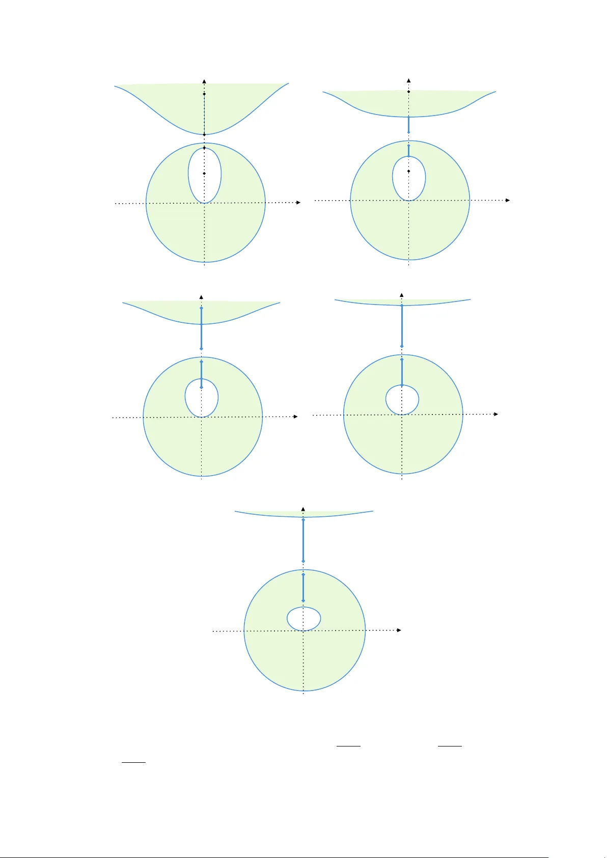
A dense fo cusing Ablo witz-Ladik soliton gas and its asymptotics Meisen Chen ∗ , Engui F an † , Zhao yu W ang §¶ , Yiling Y ang ‖ , Lun Zhang †‡ Marc h 18, 2026 Abstract In this pap er, w e prop ose a soliton gas solution for the focusing Ablowitz-Ladik system. This solution is deﬁned as the large N limit of the N -soliton solution, and arises from a con tinuous spectrum of p oles that accum ulate within tw o disjoin t interv als on the imaginary axis. W e sho w that this gas solution admits a F redholm determinan t represen tation. By further exploring its Riemann-Hilb ert c haracterization, we are able to establish the large- space asymptotics at t = 0 and large-time asymptotics of the gas solution. AMS Sub ject Cla ssiﬁcation 2020: 37K60; 39A14; 35Q51; 35B40; 35Q15; 35Q35. Con ten ts 1 In tro duction and main results 2 1.1 Main results . . . . . . . . . . . . . . . . . . . . . . . . . . . . . . . . . . . . . . . . . . 3 2 The soliton gas solution and its RH c haracterization 7 3 F redholm determinant representation of q n 12 3.1 The F redholm determinant represen tation of the N -soliton solution . . . . . . . . 12 3.2 Pro of of Theorem 1.1 . . . . . . . . . . . . . . . . . . . . . . . . . . . . . . . . . . . . 13 4 Large- n asymptotic analysis of the RH problem for Z ( λ ; n, 0 ) 15 4.1 The auxiliary functions . . . . . . . . . . . . . . . . . . . . . . . . . . . . . . . . . . . 15 4.2 Lenses op ening . . . . . . . . . . . . . . . . . . . . . . . . . . . . . . . . . . . . . . . . 18 4.3 Global parametrix . . . . . . . . . . . . . . . . . . . . . . . . . . . . . . . . . . . . . . 20 4.4 Lo cal parametrices . . . . . . . . . . . . . . . . . . . . . . . . . . . . . . . . . . . . . . 22 4.5 The small-norm RH problem . . . . . . . . . . . . . . . . . . . . . . . . . . . . . . . . 23 ∗ Sc ho ol of Mathematics and Statistics, F ujian Normal Universit y , F uzhou 350117, China. E-mail: chenms@fjnu.edu.cn. † Sc ho ol of Mathematical Sciences, F udan Universit y , Shanghai 200433, China. E-mail: { faneg, lunzhang } @fudan.edu.cn. ‡ Shanghai Key Laboratory for Contemporary Applied Mathematics, F udan Universit y , Shanghai 200433, China. § Departmen t of Mathematics, Shanghai Universit y , Shanghai 200444, China. E-mail: zhaoyuwang@shu.edu.cn. ¶ Newtouc h Center for Mathematics of Shanghai Universit y , Shanghai 200444, China. ‖ College of Mathematics and Statistics, Chongqing Univ ersity , Chongqing 401331, China. E-mail: ylyang19@fudan.edu.cn. 1 5 Large- t asymptotic analysis of the RH problem for Z ( λ ; n + 1 , t ) 24 5.1 The auxiliary functions . . . . . . . . . . . . . . . . . . . . . . . . . . . . . . . . . . . 25 5.2 Lenses op ening . . . . . . . . . . . . . . . . . . . . . . . . . . . . . . . . . . . . . . . . 29 5.3 Global parametrix . . . . . . . . . . . . . . . . . . . . . . . . . . . . . . . . . . . . . . 32 5.4 Lo cal parametrices . . . . . . . . . . . . . . . . . . . . . . . . . . . . . . . . . . . . . . 33 5.5 The small-norm RH problem . . . . . . . . . . . . . . . . . . . . . . . . . . . . . . . . 39 6 Pro ofs of the main results 41 6.1 Pro of of Theorem 1.2 . . . . . . . . . . . . . . . . . . . . . . . . . . . . . . . . . . . . 41 6.2 Pro of of Theorem 1.5 . . . . . . . . . . . . . . . . . . . . . . . . . . . . . . . . . . . . 42 A The mo del RH problems 43 A.1 The Bessel parametrix . . . . . . . . . . . . . . . . . . . . . . . . . . . . . . . . . . . . 43 A.2 The Airy parametrix . . . . . . . . . . . . . . . . . . . . . . . . . . . . . . . . . . . . . 44 A.3 The generalized Laguegrre polynomial parametrix . . . . . . . . . . . . . . . . . . . 45 A.4 The Painlev ´ e XXXIV parametrix . . . . . . . . . . . . . . . . . . . . . . . . . . . . . 46 B Unique solv ability of the equation (5.4) 47 1 In tro duction and main results The Ablowitz-Ladik (AL) system is deﬁned by i d d t q n = q n + 1 − 2 q n + q n − 1 + σ  q n  2 ( q n + 1 + q n − 1 ) , n ∈ Z , (1.1) where σ = ± 1, corresp onding to the fo cusing/defocusing case, resp ectively . The AL system was in tro duced by Ablo witz and Ladik [ 2 , 3 ] via discretizing the 2 × 2 Zakharov-Shabat Lax pair of the cubic nonlinear Schr¨ odinger equation i u t = u xx + σ  u  2 u. In addition, the AL system also p ossesses numerous ph ysical applications, ranging from the dynamics of anharmonic lattices [ 43 ], self-trapping on a dimer [ 31 ] to Heisenberg spin chains [ 28 , 37 ]. In this pap er, w e are concerned with the fo cusing AL system, i.e., σ = 1 in ( 1.1 ), whic h reads i d d t q n = q n + 1 − 2 q n + q n − 1 +  q n  2 ( q n + 1 + q n − 1 ) . (1.2) It is well known that the AL system is integrable as can b e seen from its bi-Hamiltonian structure [ 6 , 19 ]. There hav e b een intensiv e studies of ( 1.2 ) from multiple p ersp ectiv es, whic h include the initial-boundary problem [ 46 ], in verse scattering transform (IST) with nonzero bac kground [ 1 , 38 , 39 , 44 ], in tegrable decomp osition [ 23 ], quasi-p eriodic solutions [ 34 , 36 , 40 ], and large-time asymptotics in the presence of solitons [ 9 ]. Among v arious in vestigations of the fo cusing AL system, w e particularly mention the soliton solutions – one of the most fundamental types of particular solutions for in tegrable systems. In the framework of IST, these solutions are related to p oles of the transmission coeﬃcient. A one-soliton solution arises from a pair of conjugate simple p oles, while an N -soliton solution corresp onds to N pairs of conjugate simple p oles. The one-soliton solution to the AL system ( 1.2 ) asso ciated with the discrete eigenv alue λ 1 ∈ C suc h that  λ 1  > 1 is given by [ 2 , 4 ] q n ( t ) = i sinh ( 2 log  λ 1 )  λ 1  e − 2i ( − n arg λ 1 − ˜ wt − ψ + ) sec h ( 2 ( n + 1 ) log  λ 1  − ˜ v t − δ 0 ) , (1.3) 2 where the constants ˜ w , ˜ v and δ 0 dep end on λ 1 , and ψ + = − arg Λ 1 − 2 arg λ 1 ± π with Λ 1 b eing the normalizing constant; see also [ 35 ] for the higher-order soliton solution and ( 3.15 ) below for the N -soliton solution. The interpretation of soliton ensembles as particle-lik e entities has b een a catalyst for a m ultitude of no vel researc h endeav ors ever since its disco very . In [ 49 ], the notion of “soliton gas” w as ﬁrst introduced by Zakharov in the con text of Korteweg-de V ries (KdV) equation. By ev aluating the eﬃcien t modiﬁcation of the soliton velocity within a rareﬁed gas, Zakharo v deriv ed an integro-diﬀeren tial kinetic equation for the soliton gas. The kinetic equation describ es the ev olution of the sp ectral distribution function of solitons due to soliton-soliton collisions. The kinetic equation for the soliton gas has been extended to other in tegrable equations lik e focusing nonlinear Schr¨ odinger (NLS) equation [ 17 , 18 ] and defo cusing and resonan t NLS equations [ 10 ]. In addition, Dyac henk o et al. formulated a Riemann-Hilb ert (RH) problem for the soliton gas of the KdV equation in [ 16 ]. Later, Girotti et al. established large distance and large time asymptotics of KdV soliton gas dynamics in [ 24 ] via the RH approac h; see also [ 25 ] for the analysis of a dense mo diﬁed Korteweg-de V ries (mKdV) soliton gas. Although substantial adv ances hav e been ac hieved in the studies of soliton gases for con tin- uous integrable systems, the corresp onding analogue for discrete in tegrable systems, how ever, has seen very little progress. In [ 5 ], Aggarwal considered the T o da lattice ( p ( t ) ; q ( t )) at ther- mal equilibrium in the sense that the v ariables ( p i ) and ( e q i − q i + 1 ) are indep endent Gaussian and Gamma random v ariables, resp ectiv ely , which can b e in terpreted as a soliton gas of the T o da system. The present w ork represen ts the ﬁrst attempt to inv estigate the soliton gas of discrete integrable systems via the RH approach in the context of the fo cusing AL system ( 1.2 ), pioneering a large- n and large- t asymptotic analysis framework. Our main results are stated in the next section. 1.1 Main results As in the case of contin uous integrable system, the soliton gas solution of ( 1.2 ) is deﬁned as the large N limit of its N -soliton solution q [ N ] n . Here, q [ N ] n is determined b y the discrete sp ectrum consisting of the p oints i λ ± 1 j , λ j > 0, j = 1 , ⋯ , N , together with the asso ciated norming constants Λ j ∈ R ∖ { 0 } and reﬂection co eﬃcien t r ( λ ) . By taking N → ∞ , the soliton gas solution q n arises from a contin uous sp ectrum of p oles that accum ulate within the interv al Σ 1 ∪ Σ 2 , where Σ 1 ∶ = ( i η 1 , i η 2 ) , Σ 2 ∶ = ( i η − 1 2 , i η − 1 1 ) , 1 < η 1 < η 2 . (1.4) Our ﬁrst result sho ws that q n can b e expressed in terms of a F redholm determinant, whic h is a natural extension of the F redholm determinan t representation of the N -soliton solution q [ N ] n established in ( 3.15 ) b elow. Theorem 1.1. Supp ose that r ( λ ) is a p ositive and c ontinuous function on [ i η 1 , i η 2 ] and let K ∶ L 2 ( Σ 1 ) → L 2 ( Σ 1 ) b e an inte gr al op er ator deﬁne d by K n,t [ f ]( ζ ) =  i η 2 i η 1 K n,t ( s ; ζ ) f ( s ) d s, (1.5) wher e K n,t ( s ; ζ ) = −  r ( ζ ) r ( s )( − ζ s ) − n  2 e i t ( ζ + s + ζ − 1 + s − 1 ) 2 2 π ( 1 + ζ s ) is the asso ciate d kernel. Then, q n ( t ) ∶ = i n + 1 e 2i t d d t Im ln det  Id L 2 ( Σ 1 ) + K n + 1 ,t  (1.6) 3 is the soliton gas solution for the fo cusing AL system ( 1.2 ) . In addition, we have ∞  k = n ( 1 +  q k ( t ) 2 ) =  Re  det ( Id L 2 ( Σ 1 ) + K n + 2 ,t ) det ( Id L 2 ( Σ 1 ) + K n,t )  − 1 . (1.7) One cannot ev aluate the F redholm determinan ts ( 1.6 ) explicitly for ﬁxed n and t , and there- fore it is natural to try to approximate them for large n and t . W e start with the asymptotics of q n ( 0 ) as n → ±∞ . Theorem 1.2. L et q n ( t ) b e the soliton gas solution of the fo cusing AL system ( 1.2 ) deﬁne d in ( 1.6 ) . Assume that r ( λ ) is analytic and p ositive in a neighb orho o d of Σ 1 , we have q n ( 0 ) = O ( e − cn ) , n → +∞ , (1.8) wher e c is a p ositive c onstant, and q n ( 0 ) = i n + 1 2   η 2 η 1 −  η 1 η 2  nd  K ( k )(( n + 1 ) Ω + ∆ ) π , k  + O ( n − 1 ) , n → −∞ , (1.9) wher e nd ( z , k ) given in ( 6.5 ) is the subsidiary Jac obi el liptic function with mo dulus k = ( η 1 − 1 )( η 2 + 1 ) ( η 2 − 1 )( η 1 + 1 ) , (1.10) K is the c omplete el liptic inte gr al deﬁne d in ( 1.20 ) , Ω is a c onstant deﬁne d in ( 4.8 ) , and ∆ = l 2 ( 2Π ( l 2 1 , k ) − K ( k ))  ( 1 − l 2 1 )( 1 − l 2 2 )  η 2 η 1 ln r ( i s ) d s  ( η 2 − s )( s − η 1 )( s − η − 1 1 )( s − η − 1 2 ) with l j ∶ = η j − 1 η j + 1 , j = 1 , 2 . (1.11) Remark 1.3. Sinc e Σ 2 is the image of Σ 1 under the mapping λ ↦ ¯ λ − 1 , our assumption on r ( λ ) in The or em 1.2 also implies that r ( ¯ λ − 1 ) is analytic in some neighb orho o d of Σ 2 . W e ﬁnally derive large time asymptotics of q n ( t ) , whic h exhibits qualitativ ely diﬀeren t b e- ha viors in diﬀeren t regions of the ( n + 1 , t ) -half plane. Dep ending on the ratio ( n + 1 ) t , there are three main regions: one fast decaying region and tw o genus-1 hyperelliptic wa ve regions, to- gether with tw o transition regions b etw een adjacent regions, as describ ed b elow and illustrated in Figure 1 . Deﬁnition 1.4. With the constan ts k and l 1 giv en in ( 1.10 ) and ( 1.11 ), we deﬁne • the fast decaying region: ( n + 1 , t ) ∶ n + 1 t > − η 1 − η − 1 1 ln η 1  ; • the ﬁrst transition region T I : ( n + 1 , t ) ∶  ∞ m = 0 T ( m ) I  , where T ( m ) I = ( n + 1 , t ) ∶ − 2 m + 1 ln η 1 ln t t < n + 1 t + η 1 − η − 1 1 ln η 1 < − 2 m − 1 ln η 1 ln t t  with m ∈ { 0 } ∪ N ; 4 − η 1 − η − 1 1 ln η 1 ξ crit H I T I F ast decay ing r eg ion 0 n + 1 t T I I H I I Figure 1: Five diﬀerent asymptotic regions given in Deﬁnition 1.4 . • the ﬁrst genus-1 h yp erelliptic w av e region H I : ( n + 1 , t ) ∶ ξ crit < n + 1 t < − η 1 − η − 1 1 ln η 1  ; • the second transition region T I I :  ( n + 1 , t ) ∶  n + 1 t − ξ crit  < C t − 2  3  , where C is an y p ositiv e constan t; • the second genus-1 h yp erelliptic w av e region H I I :  ( n + 1 , t ) ∶ n + 1 t < ξ crit  . Here, ξ crit ∶ = η 2 + 1 η 2 + η 1 + 1 η 1 2 + − η 2 2 − 1 η 2 2 + 2 + 8 l 2 1 ( k 2 − l 2 1 )( l 2 1 − 1 )  E ( k ) K ( k ) + k 2 − l 2 1 l 2 1 − k 2 − l 4 1 l 2 1 Π ( l 2 1 ,k ) K ( k )  η 2 + η − 1 2 + 2 − 4 Π ( l 2 1 ,k ) K ( k ) , (1.12) where K , E and Π are the complete elliptic in tegrals deﬁned in ( 1.20 ) and ( 1.22 ). Large time asymptotics of q n ( t ) in these regions are sho wn in the following theorem. Theorem 1.5. Assume that r ( λ ) is analytic and p ositive in a neighb orho o d of Σ 1 . As t → +∞ , we have the fol lowing asymptotics of q n ( t ) in the r e gions given in Deﬁnition 1.4 . (1) F or n + 1 t in the fast de c aying r e gion, ther e exists a p ositive c onstant c such that q n ( t ) = O ( e − ct ) . (1.13) (2) F or n + 1 t ∈ T ( m ) I ⊆ T I , m ∈ { 0 } ∪ N , we have q n ( t ) = O  min ( e ( 2 m − 1 ) ln t + t ( n + 1 t + η 1 − η − 1 1 ln η 1 ) ln η 1 , e − ( 2 m + 1 ) ln t − t ( n + 1 t + η 1 − η − 1 1 ln η 1 ) ln η 1 ) . (1.14) (3) F or n + 1 t ∈ H I , we have q n ( t ) = e 2i t ( 1 + π ( n + 1 ) 4 t ) 2    α ( ξ ) η 1 −  η 1 α ( ξ )   nd  K ( k ( ξ ))( t Ω + ∆ ) π , k ( ξ ) + O ( t − 1 ) , (1.15) 5 wher e α ( ξ ) is a r e al-value d function deﬁne d in ( 5.3 ) with ξ = ( n + 1 ) t , nd ( z , k ( ξ )) given in ( 6.5 ) is the subsidiary Jac obi el liptic function with mo dulus k ( ξ ) = ( η 1 − 1 )( α ( ξ ) + 1 ) ( α ( ξ ) − 1 )( η 1 + 1 ) , (1.16) and Ω and ∆ ar e c onstants given in ( 5.11 ) and ( 5.18 ) , r esp e ctively. (4) F or n + 1 t ∈ T I I , we have q n ( t ) = e 2i t ( 1 + π ( n + 1 ) 4 t ) 2   η 2 η 1 −  η 1 η 2  nd  K ( k )( t Ω + ∆ ) π , k  + O ( t − 1  3 ) , (1.17) wher e k , Ω and ∆ ar e given in ( 1.16 ) , ( 5.11 ) and ( 5.18 ) , r esp e ctively. (5) F or n + 1 t ∈ H I I , we have q n ( t ) = e 2i t ( 1 + π ( n + 1 ) 4 t ) 2   η 2 η 1 −  η 1 η 2  nd  K ( k )( t Ω + ∆ ) π , k  + O ( t − 1 ) , (1.18) wher e k , Ω and ∆ ar e given in ( 1.16 ) , ( 5.11 ) and ( 5.18 ) , r esp e ctively. Since α ( ξ ) takes diﬀeren t v alues in diﬀerent regions, it is readily seen from ( 1.15 ) and ( 1.18 ) that the regions H I and H I I corresp ond to the gen us-1 hyperelliptic w a ve region with mo dulated and constan t coeﬃcients, respectively . In addition, as n + 1 t → − η 1 − η − 1 1 ln η 1 , the saddle p oin t of the phase function coalesces with the endp oin t i η 1 of Σ 1 , while as n + 1 t → ξ crit , it approaches the other endp oin t i η 2 ; see Figure 8 b elo w for an illustration. This leads to the introduction of transition regions T I and T I I , whic h requires new ingredien ts of analysis. It also explains wh y the error estimates diﬀer in the regions T I I and H I I , although the leading asymptotics are the same. In Theorem 1.5 , we only present the leading asymptotics of the soliton gas solution q n with error estimates for large t , whic h is the main fo cus of the presen t w ork. Our asymptotic analysis, leading to the pro of of the ab o v e theorem, also in principal allows us to establish correction terms explicitly in the expansion. All the ingredients for obtaining suc h results are presented, but we will not write the details down neither comment them an y further. It is worth while to men tion that detailed calculations of the sub-leading term in large time asymptotics of the soliton gas solution for the mKdV equation in the transition regions can b e found in [ 33 ]. W e emphasize that providing uniform asymptotics in transition regions is usually a diﬃcult problem, whic h is fully resolved only in some particular cases; cf. [ 8 , 14 , 42 , 45 , 48 ]. In the con text of fo cusing AL system, the analysis in transition regions T I and T I I in volv es RH problems relev an t to the generalized Laguerre p olynomial and P ainlev´ e XXXIV equation, resp ectiv ely , whic h is diﬀeren t from the classical lo cal parametrices used in other regions. The reason why w e divide T I in to diﬀerent subregions T ( m ) I is that the index m is exactly the degree of Laguerre p olynomials related to the lo cal analysis. Th us, although T I is relatively small in size, it is itself comp osed of several lay ers. It is w orth while to p oin t out that the transitional asymptotics of the mKdV equation for step-like initial data is also related to the RH problem built from Laguerre p olynomials [ 7 ], and the P ainlev´ e XXXIV transcendents play an imp ortan t role in asymptotic studies of critical b eha viors arsing from in tegrable diﬀeren tial equations [ 20 ], random unitary ensem bles [ 29 ] and orthogonal p olynomials [ 47 ]. The rest of this pap er is organized as follo ws. In Section 2 , we consider a sequence of RH problems, indexed b y N , characterizing the pure N -soliton solution q [ N ] n , whose sp ectrum is 6 conﬁned to the interv al Σ 1 ∪ Σ 2 . As N → +∞ , the soliton gas solution q n is then c haracterized b y the limiting RH problem for Z , which serves as the starting p oin t of further asymptotic analysis. In Section 3 , we in tro duce the tau-functions and establish the F redholm determinant represen tation of q [ N ] n . This structure is preserved in the large N limit, which leads to the pro of of Theorem 1.1 . W e p erform Deift-Zhou steep est descen t analysis [ 14 , 15 ] to RH problems for Z ( λ ; n, 0 ) and Z ( λ ; n + 1 , t ) in Sections 4 and 5 , resp ectiv ely . The main idea of the analysis is to transform RH problem for Z into a solv able form consisting of the global and lo cal RH problems. A k ey step in this pro cedure is to apply the g -function mechanism [ 13 ] to arrive at a global RH problem solv able in terms of the Jacobi theta function. As aforemen tioned, one needs sp ecial treatments for the analysis in the transition regions T I and T I I . The outcome of our analysis is the pro ofs of Theorems 1.2 and 1.5 , presen ted in Section 6 . Notations Throughout this paper, the follo wing notations will b e used. • The Pauli matrices: σ 1 =  0 1 1 0  , σ 2 =  0 − i i 0  , σ 3 =  1 0 0 − 1  . (1.19) F or a 2 × 2 matrix A , we also set e ˆ σ j A ∶ = e σ j A e − σ j , j = 1 , 2 , 3 . • Assume 1 − k 2 ∈ C ∖ ( −∞ , 0 ] and 1 − k 2 sin 2 m ∈ C ∖ ( −∞ , 0 ] , except that one of them may b e 0, and 1 − α 2 ∈ C ∖ 0. Then, the complete and incomplete elliptic in tegrals are deﬁned b y K ( k ) =  1 0 d s  ( 1 − s 2 )( 1 − k 2 s 2 ) , E ( k ) =  1 0  1 − k 2 s 2 1 − s 2 d s, (1.20) F ( m, k ) =  m 0 d s  ( 1 − s 2 )( 1 − k 2 s 2 ) , (1.21) Π ( α 2 , k ) =  1 0 d s ( 1 − α 2 s 2 )  ( 1 − s 2 )( 1 − k 2 s 2 ) . (1.22) • If A is a matrix, then ( A ) ij stands for its ( i, j ) -th en try . • In Sections 4 and 5 , we adopt the same notations (suc h as g , δ , T , Z ( 1 ) , Z ( ∞ ) , Z ( p ) , . . . ) during the analysis, which should be understo o d in diﬀeren t con texts. W e b eliev e this will not lead to any confusion. 2 The soliton gas solution and its RH c haracterization In this section, we review some basic results of the fo cusing AL system ( 1.2 ), including an RH problem for the N -soliton solution q [ N ] n [ 4 , 9 ]. By taking N → +∞ , we interpret the ( 1 , 2 ) -th en try of the limiting RH problem at the origin as the soliton gas solution. W e justify this claim b y c hecking that this entry indeed solv es the fo cusing AL system ( 1.2 ) and can b e obtained as the large N limit of q [ N ] n . F rom [ 9 ], it follo ws that q [ N ] n ( t ) = M 12 ( 0; n + 1 , t ) , (2.1) where M ( λ ; n, t ) solves the follo wing RH problem. 7 RH problem 2.1. • M ( λ ) = M ( λ ; n, t ) is meromorphic in C with simple p oles at { i λ j , i λ − 1 j } N j = 1 with λ j > 1. • M ( λ ) satisﬁes the residue conditions Res λ = i λ j M ( λ ) = lim λ → i λ j M ( λ )  0 0 − i Λ j e − ϕ ( λ ) 0  , Res λ = i λ − 1 j M ( λ ) = lim λ → i λ − 1 j M ( λ )  0 − i Λ j λ − 2 j e ϕ ( λ ) 0 0  , where Λ j , j = 1 , ⋯ , N , are nonzero norming constants and ϕ ( λ ) = ϕ ( λ ; n, t ) ∶ = − i t ( λ + λ − 1 − 2 ) + n ln λ. (2.2) • As λ → ∞ , we hav e M ( λ ) = I + O ( λ − 1 ) . Supp ose that r ( λ ) is p ositiv e and contin uous on [ i η 1 , i η 2 ] , and set λ j = η 1 + j − 1 N ( η 2 − η 1 ) , Λ j = r ( i λ j ) 2 π N , j = 1 , ⋯ , N . (2.3) It is then readily seen that lim N → +∞ N  j = 1 iΛ j λ − i λ j = 1 2 π i  Σ 1 i r ( s ) λ − s d s, λ ∈ C ∖ Σ 1 (2.4a) lim N → +∞ N  j = 1 iΛ j λ − 2 j λ − i λ j = 1 2 π i  Σ 2 i r ( ¯ s − 1 ) λ − s d s, λ ∈ C ∖ Σ 2 , (2.4b) where Σ i , i = 1 , 2, are deﬁned in ( 1.4 ). This, together with RH problem 2.1 , leads us to consider the following limiting RH problem. RH problem 2.2. • Z ( λ ) = Z ( λ ; n, t ) is analytic in C ∖ ( Σ 1 ∪ Σ 2 ) . • F or λ ∈ Σ 1 ∪ Σ 2 , Z ( λ ) satisﬁes the jump condition Z + ( λ ) = Z − ( λ ) J ( λ ) , where J ( λ ) =                    1 0 i r ( λ ) e − ϕ ( λ ) 1   , λ ∈ Σ 1 ,   1 i r ( ¯ λ − 1 ) e ϕ ( λ ) 0 1   , λ ∈ Σ 2 . (2.5) • As λ → ∞ , we hav e Z ( λ ) = I + O ( λ − 1 ) . Our next proposition sho ws that the ab o ve RH problem c haracterizes the soliton gas solution of the fo cusing AL system ( 1.2 ). Prop osition 2.3. Supp ose that r ( λ ) is p ositive and c ontinuous on [ i η 1 , i η 2 ] , then RH pr oblem 2.2 is uniquely solvable and satisﬁes the symmetry r elation Z ( λ ) = σ 2 Z ( 0 ) − 1 Z ( ¯ λ − 1 ) σ 2 . (2.6) 8 F urthermor e, q n ( t ) ∶ = Z 12 ( 0; n + 1 , t ) (2.7) is the soliton gas solution of the fo cusing AL system ( 1.2 ) and for any ( n, t ) ∈ Z × R , we have lim N → ∞ q [ N ] n ( t ) = q n ( t ) . (2.8) Pr o of. First, it is easy to c heck that the orientation of Σ 1 ∪ Σ 2 is rev ersed by the mapping λ → ¯ λ − 1 . Since the jump matrix satisﬁes the skew-Hermitian symmetry relation  J ( ¯ λ − 1 )  † = J ( λ ) − 1 for λ ∈ Σ 1 ∪ Σ 2 , Lemma 4.4 in [ 9 ] then guarantees that RH problem 2.2 is uniquely solv able. Next, to ensure q n deﬁned in ( 2.7 ) is a solution of the AL system ( 1.2 ), w e will sho w that, starting from Z , one can deﬁne a 2 × 2 matrix-v alued function Φ satisfying the Lax pair equations S Φ = A Φ , dΦ d t = B Φ , (2.9) where the co eﬃcien ts A and B are obtained from Z , and S is the righ t-shift op erator deﬁned b y S f ( n ) = f ( n + 1 ) . (2.10) The compatibility condition of ( 2.9 ) then gives us the AL system ( 1.2 ). T o pro ceed, w e note that the symmetry relation ( 2.6 ) reads Z ( λ ) = σ 2 Z ( 0 ) − 1 Z ( λ ) σ 2 ,  λ  = 1 , from which it follo ws that σ 2 Z ( λ ) − 1 σ 2 = Z ( λ ) − 1 σ 2 Z ( 0 ) − 1 σ 2 , Z ( 0 ) = Z ( λ ) σ 2 Z ( λ ) − 1 σ 2 . Com bining these t wo iden tities yields Z ( 0 ) = σ 2 Z ( 0 ) − 1 σ 2 . Denote Z 12 ( 0; n ) = q n − 1 , Z 22 ( 0; n ) = c n − 1 . (2.11) T ogether with the fact det [ Z ] ≡ 1, w e hav e Z 21 ( 0; n ) = q n − 1 , Z 11 ( 0; n ) = 1 +  q n − 1  2 c n − 1 . (2.12) Since e ϕ ( λ ) 2 is not analytic in C , w e introduce the z -plane by setting λ = z 2 , and deﬁne Φ ( z ) ∶ = Z ( z 2 ) e ϕ ( z 2 ) σ 3  2 , whic h admits the jump e ϕ ( z 2 ) ˆ σ 3  2 V for z 2 ∈ Σ 1 ∪ Σ 2 and satisﬁes Φ = ( I + O ( z − 2 )) e ϕ ( z 2 ) σ 3  2 as z → ∞ . Note that the jump of Φ is indep endent of n and t , the function Φ ( z ; n + 1 , t ) Φ ( z ; n, t ) − 1 z − σ 3 = Z ( z 2 ; n + 1 , t ) z σ 3 Z ( z 2 ; n, t ) − 1 z − σ 3 9 is analytic in the z -plane except for p ossible p oles at z = 0 and z = ∞ . T o analyze its behavior near these p oin ts, we denote Z ( λ ; n ) = I + Z 1  λ + O ( λ − 2 ) , λ → ∞ . As z → ∞ , w e hav e Φ ( z ; n + 1 , t ) Φ ( z ; n, t ) − 1 z − σ 3 = ( I + Z 1 ( n + 1 ) z 2 + O ( z − 4 ))( I + z σ 3 Z 1 ( n ) z − σ 3  z 2 + O ( z − 3 )) − 1 , = I +  0 − Z 1 , 12 ( n ) 0 0  + O ( z − 2 ) . As z → 0, it follo ws from ( 2.12 ) that Φ ( z ; n + 1 , t ) Φ ( z ; n, t ) − 1 z − σ 3 = ( Z ( 0; n + 1 ) + O ( z 2 ))( z σ 3 Z ( 0; n ) z − σ 3 + O ( z )) − 1 = ( Z ( 0; n + 1 ) + O ( z 2 ))  z − 2  0 0 − q n − 1 0  + O ( 1 ) = z − 2 Z ( 0; n + 1 )  0 0 − q n − 1 0  + O ( 1 ) . Consequen tly , one has Φ ( z ; n + 1 , t ) Φ ( z ; n, t ) − 1 z − σ 3 = z − 2 Z ( 0; n + 1 )  0 0 − q n − 1 0  + I +  0 − Z 1 , 12 ( n ) 0 0  , or equiv alen tly , S Φ = A Φ , (2.13) where A = z σ 3 − z − 1  q n − 1 q n Z 1 , 12 ( n ) q n − 1 c n 0  . Similarly , consider dΦ ( z ; n, t ) d t Φ ( z ; n, t ) − 1 = ( Z ( z 2 ; n, t ) e ϕ ( z 2 ; n,t ) σ 3  2 ) t e − ϕ ( z 2 ; n,t ) σ 3  2 Z ( z 2 ; n, t ) − 1 = d Z ( z 2 ; n, t ) d t Z ( z 2 ; n, t ) − 1 − i ( z 2 − 2 + z − 2 ) 2 Z ( z 2 ; n, t ) σ 3 Z ( z 2 ; n, t ) − 1 , whic h is analytic in the z -plane except for p ossible p oles at z = 0 and z = ∞ . As z → ∞ , w e hav e dΦ ( z ; n, t ) d t Φ ( z ; n, t ) − 1 = − i ( z 2 − 2 + z − 2 ) 2 ( I + Z 1 ( n ) z 2 + O ( z − 4 )) σ 3 ( I + Z 1 ( n ) z 2 + O ( z − 4 )) − 1 + O ( z − 2 ) = − i 2 z 2 σ 3 − i 2 ( − 2 σ 3 + σ 3 Z 1 ( n ) − 1 + Z 1 ( n ) σ 3 ) + O ( z − 2 ) = − i 2 ( z 2 − 2 ) σ 3 − i 2  Z 1 , 11 ( n ) + Z 1 , 22 ( n ) − 2 Z 1 , 12 ( n ) 2 Z 1 , 21 ( n ) − ( Z 1 , 11 ( n ) + Z 1 , 22 ( n ))  + O ( z − 2 ) , and as z → 0, w e hav e dΦ ( z ; n, t ) d t Φ ( z ; n, t ) − 1 = − i ( z 2 − 2 + z − 2 ) 2 ( Z ( 0; n ) + O ( z 2 )) σ 3 ( Z ( 0; n ) + O ( z 2 )) − 1 = − i ( z 2 − 2 + z − 2 ) 2 Z ( 0; n ) σ 3 Z ( 0; n ) − 1 + O ( 1 ) = − i 2 z − 2   1 + 2  q n − 1  2 − 2 1 +  q n − 1  2 c n − 1 q n − 1 2 q n − 1 c n − 1 − ( 1 + 2  q n − 1  2 )   + O ( 1 ) . 10 It thereby holds that dΦ d t = B Φ , (2.14) where B = − i 2 z − 2   1 + 2  q n − 1  2 − 2 1 +  q n − 1  2 c n − 1 q n − 1 2 q n − 1 c n − 1 − ( 1 + 2  q n − 1  2 )   − i 2 ( z 2 − 2 ) σ 3 − i 2  Z 1 , 11 ( n ) + Z 1 , 22 ( n ) − 2 Z 1 , 12 ( n ) 2 Z 1 , 21 ( n ) − ( Z 1 , 11 ( n ) + Z 1 , 22 ( n ))  . The compatibility condition of equations ( 2.13 ) and ( 2.14 ) then yields d A d t + AB = ( S B ) A. (2.15) Comparing the co eﬃcien ts of the O ( z ) and O ( z − 3 ) terms on b oth sides of ( 2.15 ), we obtain Z 1 , 21 ( n ) = q n − 1 c n , c n ( 1 +  q n − 1  2 ) = c n − 1 . (2.16) Substituting the ab o ve t wo equalities into the co eﬃcien t of the O ( z − 1 ) term in ( 2.15 ) yields the AL system ( 1.2 ). Finally , it remains to show ( 2.8 ). Let γ 1 b e a closed curv e encircling the in terv al Σ 1 in a clo c kwise manner and set γ 2 ∶ = γ − 1 1 whic h encircles Σ 2 . W e then deﬁne T M ( λ ) =                              1 0 ∑ N j = 1 iΛ j e − ϕ ( λ ) λ − i λ j 1   , λ ∈ D 1 ,    1 ∑ N j = 1 iΛ j λ − 2 j λ − i λ − 1 j e ϕ ( λ ) 0 1    , λ ∈ D 2 , I , otherwise , T Z ( λ ) =                            1 0 − ∫ Σ 1 i r ( s ) e − ϕ ( λ ) d s 2 π i ( s − λ ) 1   , λ ∈ D 1 ,   1 − ∫ Σ 2 i r ( s ) e ϕ ( λ ) d s 2 π i ( s − λ ) 0 1   , λ ∈ D 2 , I , otherwise , where D i , i = 1 , 2, denotes the region b et ween γ i and Σ i , and ˜ M ( λ ) ∶ = M ( λ ) T M ( λ ) , ˜ Z ( λ ) ∶ = Z ( λ ) T Z ( λ ) . (2.17) It is readily seen that ˜ M ( λ ) has no p ole at λ j and ˜ Z ( λ ) has no jump on Σ 1 ∪ Σ 2 . Indeed, the ﬁrst identit y in ( 2.17 ) implies that ˜ M ( λ ) may ha ve at most simple p oles at each λ j . Ho wev er, a direct computation of the residue condition at each λ j sho ws that ˜ M ( λ ) is p ole-free at λ j . On the other hand, by the Sokhotski-Plemelj formula, for an y λ ∈ Σ 1 , one has ˜ Z + ( λ ) = ˜ Z − ( λ )   1 0 ∫ Σ 1 i r ( s ) e − ϕ ( λ ) d s 2 π i ( s − λ − ) − ∫ Σ 1 i r ( s ) e − ϕ ( λ ) d s 2 π i ( s − λ + ) + i r ( λ ) e − ϕ ( λ ) 1   = ˜ Z − ( λ ) , so ˜ Z ( λ ) has no jump on Σ 1 . The same argumen t sho ws that ˜ Z ( λ ) has no jump on Σ 2 either. As a consequence, the function E ( λ ) ∶ = ˜ M ( λ ) ˜ Z ( λ ) − 1 satisﬁes an RH problem with the jump con tour given b y γ 1 ∪ γ 2 and the jump matrix J E reads J E ( λ ) − I = ˜ Z − ( λ ) T M − ( λ ) − 1 T Z − ( λ ) ˜ Z − ( λ ) − 1 − I = ˜ Z − ( λ )( T Z − ( λ ) − T M − ( λ )) ˜ Z − ( λ ) − 1 . (2.18) By ( 2.4 ), the right-hand side of ( 2.18 ) tends to zero as N → ∞ . Then, the RH problem for E is a small-norm RH problem for large N . Th us, by the small-norm RH problem theory [ 15 ], as N → ∞ , M ( 0; n, t ) → Z ( 0; n, t ) for an y ( n, t ) ∈ Z × R , which leads to ( 2.8 ). This completes the pro of of Prop osition 2.3 . 11 3 F redholm determinan t represen tation of q n In this section, w e intend to prov e Theorem 1.1 b y establishing a F redholm determinant repre- sen tation of the soliton gas solution q n . W e start with a construction of the N -soliton solution q [ N ] n in terms of F redholm determinants. 3.1 The F redholm determinan t representation of the N -soliton solution Note that the ﬁrst ro w of the solution of RH problem 2.1 is given by ( M 11 ( λ ) , M 12 ( λ )) = ( 1 , 0 ) − N  j = 1  i d j λ j ˆ β j λ − i λ j , i n + 1 e 2i t d j ˆ α j λ − i λ − 1 j  . (3.1) Here, the vectors ˆ α = ( ˆ α 1 , ⋯ , ˆ α N ) T and ˆ β =  ˆ β 1 , ⋯ , ˆ β N  T are determined by the ﬁnite linear system  I N − Ψ Ψ I N   ˆ α ˆ β  =  d 0  , (3.2) where I N is the N × N identit y matrix, d = ( d 1 , ⋯ , d N ) T , Ψ = Ψ ( n, t ) ∶ =   d j d k 1 − λ − 1 j λ − 1 k   N j,k = 1 , (3.3) with d j = d j ( n, t ) ∶ =  Λ j λ − n − 2 j e t ( λ − 1 j − λ j ) . (3.4) As it is assumed that r ( λ ) is p ositiv e on [ i η 1 , i η 2 ] , we see from ( 2.3 ) that d j > 0. Besides ( 2.1 ), w e also ha ve c [ N ] n ( t ) ∶ = ∞  k = n ( 1 +  q [ N ] n ( t ) 2 ) = M 11 ( 0; n, t ) − 1 , (3.5) whic h can b e pro v ed b y using an argumen t analogous to the deriv ation of ( 2.12 ). Since Ψ is real and symmetric, the linear system ( 3.2 ) is equiv alen t to  ˆ α ˆ β  =  ( I N + Ψ 2 ) − 1 ( I N + Ψ 2 ) − 1 Ψ − ( I N + Ψ 2 ) − 1 Ψ ( I N + Ψ 2 ) − 1   d 0  . (3.6) Note that I N + Ψ 2 = ( I N + iΨ )( I N − iΨ ) , we introduce the tau-function τ [ N ] ( η ) = τ [ N ] ( η ; n, t ) ∶ = det ( I N − η Ψ ( n, t )) , N ≥ 1 . (3.7) Using the fact that Ψ j k − ( S 2 Ψ ) j k = d j d k − ( S 2 d ) j ( S 2 d ) k 1 − λ − 1 j λ − 1 k = d j d k = ( dd T ) j k , (3.8) where S is the righ t-shift op erator deﬁned in ( 2.10 ), w e obtain from the W einstein–Aronsza jn iden tity that S 2 τ [ N ] ( η ) = det ( I N − η S 2 Ψ ) = τ [ N ] ( η ) det ( I N + η ( I N − η Ψ ) − 1 ( Ψ − S 2 Ψ )) = τ [ N ] ( η ) det ( I N + η ( I N − η Ψ ) − 1 dd T ) = τ [ N ] ( η )( 1 + η d T ( I N − η Ψ ) − 1 d ) , 12 whic h yields S 2 τ [ N ] ( η ) τ [ N ] ( η ) = 1 + η d T ( I N − η Ψ ) − 1 d . (3.9) In addition, by Jacobi’s form ula, we ha ve d d t ln τ [ N ] ( η ) = T r [ − η ( I N − η Ψ ) − 1 d d t Ψ ] . (3.10) In view of ( 3.3 ), it follo ws that d d t Ψ j k = − λ j + λ k 2 d j d k . (3.11) Substituting ( 3.11 ) in to ( 3.10 ) giv es us d d t ln τ [ N ] ( η ) = η 2 d T [ D ( I N − η Ψ ) − 1 + ( I N − η Ψ ) − 1 D ] d = η d T D ( I N − η Ψ ) − 1 d , (3.12) where D ∶ = diag ( λ 1 , ⋯ , λ N ) . T aking η = i in ( 3.12 ) and extracting the imaginary part yields d d t Im ln τ [ N ] ( i ) = 1 2i  d d t ln τ [ N ] ( i ) − d d t ln τ [ N ] ( i ) = d T D ( I N + Ψ 2 ) − 1 d . (3.13) On the other hand, it follo ws from ( 3.1 ) that M 12 ( 0; n, t ) = i n e 2i t N  j = 1 λ j d j ( n, t ) ˆ α j ( n, t ) = i n e 2i t [ d T D ( I N + Ψ 2 ) − 1 d ]( n, t ) , (3.14) whic h combined with ( 2.1 ) and ( 3.13 ) induces q [ N ] n ( t ) = i n + 1 e 2i t d d t Im ln τ [ N ] ( i; n + 1 , t ) . (3.15) Similarly , using ( 3.1 ), ( 3.5 ), ( 3.8 ) and ( 3.9 ), it follows that  c [ N ] n ( t ) − 1 = 1 + d ( n, t ) T ˆ β ( n, t ) = 1 − d ( n, t ) T ( I + Ψ ( n, t ) 2 ) − 1 Ψ ( n, t ) d ( n, t ) = 1 2  τ [ N ] ( − i; n + 2 , t ) τ [ N ] ( − i; n, t ) + τ [ N ] ( i; n + 2 , t ) τ [ N ] ( i; n, t )  = Re  τ [ N ] ( i; n + 2 , t ) τ [ N ] ( i; n, t )  . (3.16) W e are now ready to prov e Theorem 1.1 . 3.2 Pro of of Theorem 1.1 By ( 3.4 ), it is readily seen that d j ( n + 2 , t ) = λ − 1 j d j ( n, t ) . This inspires us to consider the tau-function in ( 3.7 ) for diﬀerent parity of n . F or the tau- function asso ciated with Ψ ( 2 n, t ) , deﬁne the linear op erators A N ,e n,t ∶ ℓ 2 ({ l } ∞ l = n ) → C N , B N ,e n,t ∶ C N → ℓ 2 ({ l } ∞ l = n ) 13 b y ( A N ,e n,t [ x ]) j = ∞  l = n d j ( 2 l, t ) x ( l ) , B N ,e n,t [ u ]( l ) = − i N  j = 1 d j ( 2 l, t ) u j , (3.17) for j = 1 , ⋯ , N and l ∈ Z ≥ n . Thu s, b y ( 3.3 ), one has − iΨ ( 2 n, t ) = A N ,e n,t ○ B N ,e n,t . Using the fact that det ( I N + A N ,e n,t ○ B N ,e n,t ) = det ( Id ℓ 2 ({ l } ∞ l = n ) + B N ,e n,t ○ A N ,e n,t ) , we obtain from ( 3.15 ), ( 3.7 ) and the ab ov e form ula that q [ N ] 2 n − 1 ( t ) = ( − 1 ) n e 2i t d d t Im ln τ [ N ] ( i; 2 n, t ) = ( − 1 ) n e 2i t d d t Im ln det ( I N + A N ,e n,t ○ B N ,e n,t ) = ( − 1 ) n e 2i t d d t Im ln det ( Id ℓ 2 ({ l } ∞ l = n ) + K N ,e n,t ) , where K N ,e n,t ∶ = B N ,e n,t ○ A N ,e n,t . Note that K N ,e n,t is a discrete in tegral operator acting on ℓ 2 ({ l } ∞ l = n ) with kernel ∑ N k = 1 d k ( l + l ′ , t ) 2 , that is, K N ,e n,t [ x ]( l ) ∶ = − i ∞  l ′ = n N  k = 1 d k ( l + l ′ , t ) 2 x ( l ′ ) . (3.18) Let N → ∞ , b y equations ( 2.3 ) and ( 2.4 ), it follows that lim N → ∞ N  k = 1 d k ( l + l ′ , t ) 2 = 1 2 π i  Σ 1 r ( s )( − i s ) − l − l ′ − 2 e i t ( s + s − 1 ) d s, (3.19) whic h implies that sequence of op erators K N ,e n,t con verges to the op erator K e n,t on ℓ 2 ({ l } ∞ l = n ) whose kernel is giv en by the righ t-hand side of ( 3.19 ). Consequen tly , lim N → ∞ det ( Id ℓ 2 ({ l } ∞ l = n ) + K N ,e n,t ) = det ( Id ℓ 2 ({ l } ∞ l = n ) + K e n,t ) , (3.20) where K e n,t = B e n,t ○ A e n,t with A e n,t [ f ]( s ) =  r ( s ) ∞  l = n ( − i s ) − l − 1 e i t 2 ( s + s − 1 ) f ( l ) , (3.21) B e n,t [ g ]( l ) = − 1 2 π  Σ 1  r ( s )( − i s ) − l − 1 e i t 2 ( s + s − 1 ) g ( s ) d s. (3.22) Again using det ( Id ℓ 2 ({ l } ∞ l = n ) + B e n,t ○ A e n,t ) = det ( Id L 2 ( Σ 1 ) + A e n,t ○ B e n,t ) , we arrive at ( 1.6 ) for ev en n . The same argument applies for the tau-function asso ciated with Ψ ( 2 n − 1 , t ) . Replacing A N ,e n,t and B N ,e n,t in ( 3.17 ) by A N ,o n,t and B N ,o n,t with ( A N ,o n,t [ x ]) j = ∞  l = n d j ( 2 l − 1 , t ) x ( l ) , B N ,o n,t [ u ]( l ) = − i N  j = 1 d j ( 2 l − 1 , t ) u j . 14 T aking the limit N → ∞ yields ( 1.6 ) for o dd n , where K 2 n − 1 ,t ∶ = A o n,t ○ B o n,t with A o n,t [ f ]( s ) =  r ( s ) ∞  l = n ( − i s ) − l − 1 2 e i t 2 ( s + s − 1 ) f ( l ) , B o n,t [ g ]( l ) = − 1 2 π  Σ 1  r ( s )( − i s ) − l − 1 2 e i t 2 ( s + s − 1 ) g ( s ) d s. The form ula ( 1.7 ) for c n ( t ) = ∏ ∞ k = n ( 1 +  q n  2 ) follo ws directly by expressing c [ N ] n ( t ) in ( 3.5 ) as a F redholm determinan t and setting N → ∞ . This completes the pro of of Theorem 1.1 . 4 Large- n asymptotic analysis of the RH problem for Z ( λ ; n, 0 ) F rom the reconstruction form ula ( 2.7 ), we ha ve q n ( 0 ) = Z 12 ( 0; n + 1 , 0 ) , (4.1) where Z solves RH problem 2.2 . This inspires us to analyze the large- n b eha vior of Z ( λ ; n + 1 , 0 ) . If t = 0, one has ϕ ( λ ; n, 0 ) = n ln λ, whic h we denote b y ϕ ( λ ) in this section for brevity . Thus, the jump matrix J of Z decays exp onen tially to the iden tity matrix as n → +∞ in this case, so do es Z ( λ ) for large positive n . In what follows, we analyze the RH problem 2.2 for Z ( λ ; n, 0 ) as n → −∞ and b egin with the introduction of some auxiliary functions, whic h particularly include the so-called g -function [ 13 , 26 , 27 ] to con trol the exp onen tially growing oﬀ-diagonal factors in the jump matrix. 4.1 The auxiliary functions T o deﬁne the g -function, w e ﬁrst in tro duce R ( λ ) ∶ =  ( λ − i η 1 )( λ − i η 2 )( λ − i η − 1 1 )( λ − i η − 1 2 ) , (4.2) whic h determines a ge n us-1 Riemann surface R with homology basis { a , b } as sho wn in Figure 2 . Note that the branc h cuts of R ( λ ) are Σ 1 ∪ Σ 2 , w e choose the principal sheet suc h that, as λ → ∞ , R ( λ ) = − λ 2 + O ( λ ) , and R ( λ ) satisﬁes the symmetry relation R ( λ ) = − λ 2 R ( ¯ λ − 1 ) . (4.3) Th us, w e ha ve R ( 0 ) = 1 and R ( λ ) > 0 for λ ∈ i ( −∞ , η − 1 2 ) ∪ i ( η 2 , +∞ ) . In addition, R ± ( λ ) ∈ i R ± for λ ∈ Σ 1 while R ± ( λ ) ∈ i R ∓ for λ ∈ Σ 2 . Next we deﬁne g ( λ ) ∶ = − 1 2  λ i η 2 s − s − 1 − i κ 1 R ( s ) d s, (4.4) where κ 1 = 2  2Π ( l 2 1 , k ) K ( k ) − 1  , l j = η j − 1 η j + 1 , k = l 1 l 2 , j = 1 , 2 , (4.5) with K and Π b eing the elliptic in tegrals deﬁned in ( 1.20 ) and ( 1.22 ), resp ectively . 15 i η 2 i η 1 i η − 1 1 i η − 1 2 Sheet I Sheet I I b a Figure 2: The genus-1 Riemann surface R with homology basis { a , b } associated with R ( λ ) in ( 4.2 ), where Sheet I is the principal sheet, and the curves Σ 1 and Σ 2 are the branch cuts. Prop osition 4.1. The g -function deﬁne d in ( 4.4 ) satisﬁes the fol lowing pr op erties. (a) L et d g b e the diﬀer ential of g ( λ ) , it then fol lows that  i η 1 i η − 1 1 d g = 0 . (b) g ( λ ) − ln λ 2 is analytic in C ∖ Σ , wher e Σ ∶ = i ( η − 1 2 , η 2 ) (4.6) with upwar d orientation and the br anch cut of the lo garithmic function is taken along the ne gative imaginary axis. Mor e over, one has g + ( λ ) =        − g − ( λ ) , λ ∈ Σ 1 ∪ Σ 2 , g − ( λ ) − iΩ , λ ∈ i ( η − 1 1 , η 1 ) , (4.7) wher e Ω = i  b d g ∈ R . (4.8) (c) g ( λ ) satisﬁes the symmetry r elation g ( ¯ λ − 1 ) = − g ( λ ) . (4.9) (d) g ( λ ) admits the asymptotic pr op erties: g ( λ ) = ln λ 2 + O ( 1 ) , λ → ∞ , (4.10) g ( λ ) = ( η 2 + η − 1 2 − κ 1 )( − i λ − η 2 ) 1  2  ( η 2 − η 1 )( η 2 − η − 1 1 )( η 2 − η − 1 2 ) ( 1 + O ( λ − i η 2 )) , λ → i η 2 , (4.11) 16 and as λ → i η 1 , g ( λ ) = ∓ iΩ 2 + ( η 1 + η − 1 1 − κ 1 )( η 1 + i λ ) 1  2  ( η 2 − η 1 )( η 1 − η − 1 1 )( η 1 − η − 1 2 ) ( 1 + O ( λ − i η 1 )) , ∓ Re λ > 0 . (4.12) Pr o of. By direct computations, w e hav e  i η 1 i η − 1 1 1 R ( s ) d s = − i  η 1 η − 1 1 1  ( s − η 1 )( s − η − 1 1 )( s − η 2 )( s − η − 1 2 ) d s = − i 2  l 1 − l 1     ( 1 − l 2 1 )( 1 − l 2 2 ) ( l 2 1 − x 2 )( l 2 2 − x 2 ) d x = − i  ( 1 − l 2 1 )( 1 − l 2 2 ) l 2 K ( k ) , (4.13) where K is deﬁned in ( 1.20 ), and  i η 1 i η − 1 1 s − s − 1 R ( s ) d s =  η 1 η − 1 1 s + s − 1  ( s − η 1 )( s − η − 1 1 )( s − η 2 )( s − η − 1 2 ) d s =  l 1 − l 1     ( 1 − l 2 1 )( 1 − l 2 2 ) ( l 2 1 − x 2 )( l 2 2 − x 2 ) ⋅ ( 1 + x 2 ) d x 1 − x 2 = 2  ( 1 − l 2 1 )( 1 − l 2 2 ) l 2 ( 2Π ( l 2 1 , k ) − K ( k )) . (4.14) Th us, the c hoice of κ 1 in ( 4.5 ) ensures item (a). Item (b) follo ws immediately the deﬁnition of g ( λ ) , ( 4.13 ) and ( 4.14 ). The symmetry relation of g in item (c) follows directly from that of R giv en in ( 4.3 ). F or item (d), it is readily seen from the deﬁnition of g in ( 4.4 ) that g ( λ ) − ln λ 2 is b ounded as λ → ∞ . The remaining statements, namely ( 4.11 ) and ( 4.12 ), are veriﬁed as follo ws. F rom the jump condition for g ( λ ) given in ( 4.7 ), it follows that g ( λ )( λ − i η 2 ) − 1  2 is holomorphic at λ = i η 2 , where the branc h cut of ( λ − i η 2 ) 1  2 is tak en along ( i η 2 , − i ∞ ) . A direct computation using L’Hˆ opital’s rule yields lim λ → i η 2 g ( λ )( − i λ − η 2 ) − 1  2 = η 2 + η − 1 2 − κ 1  ( η 2 − η 1 )( η 2 − η − 1 1 )( η 2 − η − 1 2 ) , whic h is equiv alen t to ( 4.11 ). A similar analysis leads to ( 4.12 ). This completes the pro of of Prop osition 4.1 . The signature table of Re [ g ] is illustrated in Figure 3 and w e also set g ( ∞ ) ∶ = lim λ → ∞  g ( λ ) − ln λ 2  . (4.15) for later use. Besides the g -function deﬁned in ( 4.4 ), w e further in tro duce an auxiliary function δ ( λ ) ∶ = exp  R ( λ ) 2 π i   i η 2 i η 1 ln r ( s ) R + ( s ) d s s − λ −  i η − 1 1 i η − 1 2 ln r ( ¯ s − 1 ) R + ( s ) d s s − λ −  i η 1 i η − 1 1 i∆ R ( s ) d s s − λ  , (4.16) where ∆ ∶ = 2i  i η 2 i η 1 ln r ( s ) R + ( s ) d s   i η 1 i η − 1 1 d s R ( s ) = − 2 l 2 ∫ η 2 η 1 ln r ( i s )  R + ( s ) d s  ( 1 − l 2 1 )( 1 − l 2 2 ) K ( k ) (4.17) 17 i η − 1 1 i η 2 i η − 1 2 i η 1 + Figure 3: The signature table of Re [ g ] . Re [ g ] > 0 in the green region, while Re [ g ] < 0 in the white region, and Re [ g ] = 0 on the blue curve. is a real constant to guarantee the boundedness of δ ( λ ) as λ → ∞ . It is readily seen from its deﬁnition that δ ( λ ) is analytic for λ ∈ C ∖ Σ and admits the jump relations δ + ( λ ) =            δ − ( λ ) − 1 r ( λ ) , λ ∈ Σ 1 , δ − ( λ ) − 1 r ( ¯ λ − 1 ) − 1 , λ ∈ Σ 2 , δ − ( λ ) e − i∆ , λ ∈ i ( η − 1 1 , η 1 ) . (4.18) Substituting λ → ¯ λ − 1 in to ( 4.16 ), one immediately veriﬁes the symmetry relation δ ( ¯ λ − 1 ) = δ ( λ ) − 1 . (4.19) Moreo ver, one has δ ( ∞ ) ∶ = lim λ → ∞ δ ( λ ) = exp  1 2 π i   i η 2 i η 1 s ln r ( s ) R + ( s ) d s −  i η − 1 1 i η − 1 2 s ln r ( ¯ s − 1 ) R + ( s ) d s −  i η 1 i η − 1 1 i∆ s R ( s ) d s  ∈ R . (4.20) 4.2 Lenses op ening With the functions g and δ deﬁned in ( 4.4 ) and ( 4.16 ), we now deﬁne T ( λ ) = T ( λ ; n ) = δ ( ∞ ) σ 3 e ng ( ∞ ) σ 3 Z ( λ ) e − n ( g ( λ ) − ln λ 2 ) σ 3 δ ( λ ) − σ 3 , (4.21) where g ( ∞ ) is given in ( 4.15 ). It is then readily seen from RH problem 2.2 , Prop osition 4.1 , ( 4.18 ) and ( 4.20 ) that T solves the follo wing RH problem. RH problem 4.2. • T ( λ ) is analytic in C ∖ Σ. 18 • F or λ ∈ Σ, T satisﬁes the jump condition T + ( λ ) = T − ( λ ) J ( T ) ( λ ) , where J ( T ) ( λ ) = J ( T ) ( λ ; n ) ∶ =                          r ( λ ) − 1 δ − ( λ ) 2 e 2 ng − ( λ ) 0 i r ( λ ) − 1 δ + ( λ ) 2 e 2 ng + ( λ )   , λ ∈ Σ 1 ,   r ( ¯ λ − 1 ) − 1 δ + ( λ ) − 2 e − 2 ng + ( λ ) i 0 r ( ¯ λ − 1 ) − 1 δ − ( λ ) − 2 e − 2 ng − ( λ )   , λ ∈ Σ 2 , e i ( n Ω + ∆ ) σ 3 , λ ∈ i ( η − 1 1 , η 1 ) . (4.22) • As λ → ∞ , we hav e T ( λ ) = I + O ( λ − 1 ) . F or λ ∈ Σ 1 ∪ Σ 2 , it is noticed that J ( T ) admits the following factorizations: J ( T ) ( λ ) =                    1 − i r ( λ ) − 1 δ − ( λ ) 2 e 2 ng − ( λ ) 0 1     0 i i 0     1 − i r ( λ ) − 1 δ + ( λ ) 2 e 2 ng + ( λ ) 0 1   , λ ∈ Σ 1 ,   1 0 − i r ( ¯ λ − 1 ) − 1 δ − ( λ ) − 2 e − 2 ng − ( λ ) 1     0 i i 0     1 0 − i r ( ¯ λ − 1 ) − 1 δ + ( λ ) − 2 e − 2 ng + ( λ ) 1   , λ ∈ Σ 2 . This in vok es us to op en lenses around the interv al Σ 1 ∪ Σ 2 . T o pro ceed, let Ω 1 , ± b e tw o regions surrounding Σ 1 and set Ω 2 , ± = Ω − 1 1 , ∓ ; see Figure 4 for an illustration. By in tro ducing a matrix-v alued function G ( λ ) = G ( λ ; n ) ∶ =                          1 ± ie 2 ng ( λ ) δ ( λ ) 2 r ( λ ) − 1 0 1   , λ ∈ Ω 1 , ± ,   1 0 ± ie − 2 ng ( λ ) δ ( λ ) − 2 r ( ¯ λ − 1 ) − 1 1   , λ ∈ Ω 2 , ± , I , otherwise , (4.23) w e deﬁne Z ( 1 ) ( λ ) = Z ( 1 ) ( λ ; n ) = T ( λ ) G ( λ ) . (4.24) Recall that r ( λ ) is analytic and p ositiv e in a neighborho o d of Σ 1 ∪ Σ 2 , w e ha ve that Z satisﬁes the following RH problem. RH problem 4.3. • Z ( 1 ) ( λ ) is analytic in C ∖ Σ ( 1 ) , where the jump con tour Σ ( 1 ) is shown in Figure 4 . • F or λ ∈ Σ ( 1 ) , Z ( 1 ) ( λ ) satisﬁes the jump condition Z ( 1 ) + ( λ ) = Z ( 1 ) − ( λ ) J ( 1 ) ( λ ) , where J ( 1 ) ( λ ) =                                      1 − ie 2 ng ( λ ) δ ( λ ) 2 r ( λ ) − 1 0 1   , λ ∈ Γ 1 ,   1 0 − ie − 2 ng ( λ ) δ ( λ ) − 2 r ( ¯ λ − 1 ) − 1 1   , λ ∈ Γ 2 ,   0 i i 0   , λ ∈ Σ 1 ∪ Σ 2 , e i ( n Ω + ∆ ) σ 3 , λ ∈ i ( η − 1 1 , η 1 ) . (4.25) 19 Ω 1 , + Ω 1 , − Ω 2 , + Ω 2 , − Γ 1 Γ 2 i η − 1 2 i η − 1 1 i η 1 i η 2 Figure 4: The regions Ω i, ± , i = 1 , 2, and the jump contour Σ ( 1 ) of Z ( 1 ) . • As λ → ∞ , we hav e Z ( 1 ) ( λ ) = I + O ( λ − 1 ) . F rom the signature table of Re [ g ] in Figure 3 , it is easily seen that the jump matrix J ( 1 ) deca ys exp onen tially to I on Γ 1 ∪ Γ 2 as n → −∞ except the endp oin ts. It inspires us to ignore the jump a wa y from Σ = i ( η − 1 2 , η 2 ) and appro ximate Z ( 1 ) in global and local manners. More precisely , let U ( p ) ∶ = { λ ∶  λ − p  ≤ ϵ } , p = i η j , j = 1 , 2 , (4.26) where ϵ is a suﬃcien tly small p ositive constant, and U ( p ) ∶ = U ( ¯ p − 1 ) − 1 , p = i η − 1 j , j = 1 , 2 . (4.27) In what follows, w e will construct the global parametrix Z ( ∞ ) ( λ ) in Section 4.3 and the lo cal parametrix Z ( p ) ( λ ) near p = i η ± 1 1 , i η ± 1 2 , in Section 4.4 suc h that Z ( 1 ) ( λ ) =        E ( λ ) Z ( ∞ ) ( λ ) , λ ∈ C ∖ U, E ( λ ) Z ( p ) ( λ ) , λ ∈ U ( p ) , p = i η ± 1 1 , i η ± 1 2 , (4.28) where U ∶ =  p = i η ± 1 1 , i η ± 1 2 U ( p ) and E ( λ ) is an error function satisfying a small norm RH problem as sho wn in Section 4.5 . 4.3 Global parametrix The global parametrix is obtained b y ignoring the jump of Z ( 1 ) oﬀ Σ, which reads as follo ws. RH problem 4.4. • Z ( ∞ ) ( λ ) = Z ( ∞ ) ( λ ; n ) is analytic in C ∖ Σ. 20 • F or λ ∈ Σ, Z ( ∞ ) ( λ ) satisﬁes the jump conditions Z ( ∞ ) + ( λ ) = Z ( ∞ ) − ( λ ) J ( ∞ ) ( λ ) , where J ( ∞ ) ( λ ) =              0 i i 0   , λ ∈ Σ 1 ∪ Σ 2 , e i ( n Ω + ∆ ) σ 3 , λ ∈ i ( η − 1 1 , η 1 ) . • As λ → ∞ , we hav e Z ( ∞ ) ( λ ) = I + O ( λ − 1 ) . T o solve the ab o v e RH problem, w e start with the normalized Ab el diﬀerential giv en by ω ( λ ) = i l 2 2 K ( k )  ( 1 − l 2 1 )( 1 − l 2 2 ) d λ R ( λ ) , where k is shown in ( 4.5 ), and deﬁne the Ab el-Jacobi map A ( λ ) =  λ i η 2 ω , λ ∈ C ∖ Σ , (4.29) where the path of integration is on an y simple arc from i η 2 to λ which do es not in tersect Σ. By direct calculations, we ha ve A + ( i η 1 ) = − τ 2 , A + ( i η − 1 1 ) = − τ 2 − 1 2 , A +  i ( η 1 + η 2 ) 1 + η 1 η 2  = A ( 0 ) − τ 2 , A ( 0 ) = − 1 4  1 + F ( arcsin l 2 , k ) K ( k )  , where τ ∶ =  b ω = i l 2 K ( k )  ( 1 − l 2 1 )( 1 − l 2 2 )  i η 2 i η 1 d s R ( s ) = i K ( √ 1 − k 2 ) 2 K ( k ) ∈ i R + is the b -p eriod and F is deﬁned in ( 1.22 ). In addition, it is straigh tforw ard to chec k from the deﬁnition of A that A ( ¯ λ − 1 ) + A ( λ ) = − 1 2 , (4.30) and A + ( λ ) =            − A − ( λ ) , λ ∈ Σ 1 , A − ( λ ) − τ , λ ∈ i ( η − 1 1 , η 1 ) , − A − ( λ ) + 1 , λ ∈ Σ 2 . (4.31) Next, we introduce a scalar function κ ( λ ) ∶ =  λ − i η 2 λ − i η 1  1 4  λ − i  η 1 λ − i  η 2  1 4 , λ ∈ C ∖ ( Σ 1 ∪ Σ 2 ) , (4.32) where the branc h cut is c hosen such that κ ( λ ) → 1 as λ → ∞ . Moreo ver, it is noted that κ ( λ ) − κ ( λ ) − 1 has a simple zero at λ = i η 1 + η 2 1 + η 1 η 2 , and one has κ + ( λ ) = i κ − ( λ ) , λ ∈ Σ 1 ∪ Σ 2 . (4.33) 21 With the aid of the scalar functions A ( λ ) and κ ( λ ) , w e deﬁne Z ( ∞ ) 11 ( λ ) = ( κ ( λ ) + 1  κ ( λ )) ϑ ( A ( λ ) + A ( 0 ) + 1 2 + n Ω + ∆ 2 π , τ ) ϑ ( 0 , τ ) 2 ϑ ( A ( λ ) + A ( 0 ) + 1 2 , τ ) ϑ ( n Ω + ∆ 2 π , τ ) , (4.34a) Z ( ∞ ) 12 ( λ ) = ( κ ( λ ) − 1  κ ( λ )) ϑ ( − A ( λ ) + A ( 0 ) + 1 2 + n Ω + ∆ 2 π , τ ) ϑ ( 0 , τ ) 2 ϑ ( − A ( λ ) + A ( 0 ) + 1 2 , τ ) ϑ ( n Ω + ∆ 2 π , τ ) , (4.34b) Z ( ∞ ) 21 ( λ ) = ( κ ( λ ) − 1  κ ( λ )) ϑ ( A ( λ ) − A ( 0 ) − 1 2 + n Ω + ∆ 2 π , τ ) ϑ ( 0 , τ ) 2 ϑ ( A ( λ ) − A ( 0 ) − 1 2 , τ ) ϑ ( n Ω + ∆ 2 π , τ ) , (4.34c) Z ( ∞ ) 22 ( λ ) = ( κ ( λ ) + 1  κ ( λ )) ϑ ( − A ( λ ) − A ( 0 ) − 1 2 + n Ω + ∆ 2 π , τ ) ϑ ( 0 , τ ) 2 ϑ ( − A ( λ ) − A ( 0 ) − 1 2 , τ ) ϑ ( n Ω + ∆ 2 π , τ ) , (4.34d) where ϑ ( λ, τ ) is the Riemann theta function deﬁned b y the F ourier series ϑ ( λ, τ ) =  l ∈ Z e 2 π i lλ + π i l 2 τ , λ ∈ C (4.35) asso ciated with τ . Note that ϑ ( λ, τ ) has a simple zero at λ = τ + 1 2 . F rom ( 4.29 ), ( 4.32 ) and ( 4.35 ), it follows that Z ( ∞ ) ( λ ) is analytic in C ∖ Σ, and by ( 4.31 ) and ( 4.33 ), Z ( ∞ ) ( λ ) satisﬁes the jump condition of RH problem 4.4 . Since κ → 1 as λ → ∞ , this, together with the symmetry relation ( 4.30 ), implies that Z ( ∞ ) ( λ ) → I . Thus, Z ( ∞ ) ( λ ) in ( 4.34 ) indeed solv es RH problem 4.4 and, in addition, satisﬁes the symmetry relation Z ( ∞ ) ( λ ) = σ 2 Z ( ∞ ) ( 0 ) − 1 Z ( ∞ ) ( ¯ λ − 1 ) σ 2 . (4.36) 4.4 Lo cal parametrices Let p = i η ± 1 j , j = 1 , 2, and U ( p ) deﬁned in ( 4.26 ) and ( 4.27 ) b e a small disc cen tered at p . The lo cal paramertix in each U ( p ) reads as follo ws. RH problem 4.5. • Z ( p ) ( λ ) = Z ( p ) ( λ ; n ) is analytic in U ( p ) ∖ ( Γ 1 ∪ Γ 2 ∪ Σ ) . • F or λ ∈ U ( p ) ∩ ( Γ 1 ∪ Γ 2 ∪ Σ ) , Z ( p ) ( λ ) satisﬁes the jump condition Z ( p ) + ( λ ) = Z ( p ) − ( λ ) ×                                      1 − ie 2 ng ( λ ) δ ( λ ) 2 r ( λ ) − 1 0 1   , λ ∈ Γ 1 ∩ U ( p ) ,   1 0 − ie − 2 ng ( λ ) δ ( λ ) − 2 r ( ¯ λ − 1 ) − 1 1   , λ ∈ Γ 2 ∩ U ( p ) ,   0 i i 0   , λ ∈ ( Σ 1 ∪ Σ 2 ) ∩ U ( p ) , e i ( n Ω + ∆ ) σ 3 , λ ∈ i ( η − 1 1 , η 1 ) ∩ U ( p ) . (4.37) • As n → −∞ , Z ( p ) ( λ ) matches Z ( ∞ ) ( λ ) on the b oundary ∂ U ( p ) . The RH problem for Z ( p ) can b e solved explicitly with the aid of the Bessel parametrix in tro duced in App endix A.1 . W e give a sk etch of the construction in what follows. F or p = i η 2 , deﬁne ζ = ζ ( λ ) ∶ = g ( λ ) 2 . (4.38) 22 By ( 4.11 ), it is easily seen that ζ ( λ ) is analytic in U ( i η 2 ) and ζ ( i η 2 ) = 0. The lo cal paramatrix around λ = i η 2 is given by Z ( i η 2 ) ( λ ) = A ( λ ) Ψ Bes  n 2 ζ 4  σ 1 e n √ ζ σ 3   δ ( λ ) e − π i 4  r ( λ )   − σ 3 , (4.39) where Ψ Bes deﬁned in ( A.2 ) is the Bessel parametrix and A ( λ ) = Z ( ∞ ) ( λ ) √ 2   δ ( λ ) e − π i 4  r ( λ )   σ 3  − i 1 1 − i  ( − nπ  ζ ) σ 3 2 with Z ∞ and δ given in ( 4.34 ) and ( 4.16 ), resp ectiv ely . Since A ( λ ) has no jump in U ( i η 2 ) and admits at most − 1 4 -singularit y at λ = i η 2 , it follo ws that A ( λ ) is an analytic prefactor. In view of RH problem A.1 for Ψ Bes , one can c heck directly that Z ( i η 2 ) in ( 4.39 ) solv es RH problem 4.5 with p = i η 2 . Similarly , for λ ∈ U ( i η 1 ) , we introduce ζ = ζ ( λ ) ∶ =  g ( λ ) ± iΩ 2  2 , ± Re λ > 0 , (4.40) and Z ( i η 1 ) ( λ ) ∶ = A ( λ ) Ψ Bes  n 2 ζ 4  σ 1 e ( − n √ ζ ± iΩ 2 ) σ 3   δ ( λ ) e − π i 4  r ( λ )   − σ 3 , (4.41) where A ( λ ) = Z ( ∞ ) ( λ ) √ 2 e ∓ iΩ 2 σ 3   δ ( λ ) e − i π 4  r ( λ )   σ 3  − i 1 1 − i  ( − nπ  ζ ) σ 3 2 , solv es RH problem 4.5 with p = i η 1 . Meanwhile, near i η − 1 j , j = 1 , 2, the lo cal parametrix can b e constructed through the symmetry relation Z ( i η − 1 j ) ( λ ) = σ 2 Z ( ∞ ) ( 0 ) − 1 Z ( i η j ) ( ¯ λ − 1 ) σ 2 . (4.42) Finally , we note from ( 4.34 ), ( 4.39 ), ( 4.41 ), ( 4.42 ) and ( A.1 ) that as n → −∞ , Z ( p ) ( λ ) Z ( ∞ ) ( λ ) − 1 = I + O ( n − 1 ) , λ ∈ ∂ U ( p ) . (4.43) 4.5 The small-norm RH problem In view of RH problems for Z ( 1 ) , Z ( ∞ ) and Z ( p ) , it is readily seen that the error function (see ( 4.28 )) E ( λ ) =  Z ( 1 ) ( λ ) Z ( ∞ ) ( λ ) − 1 , λ ∈ C ∖ U, Z ( 1 ) ( λ ) Z ( p ) ( λ ) − 1 , λ ∈ U ( p ) , p = i η ± 1 1 , i η ± 1 2 , (4.44) satisﬁes the following RH problem. RH problem 4.6. • E ( λ ) is analytic in C ∖ Σ E , where the contour Σ E is shown in Figure 5 . 23 U ( i η 2 ) U ( i η 1 ) U ( i η − 1 1 ) U ( i η − 1 2 ) Figure 5: The jump con tour Σ E of E . • F or λ ∈ Σ E , E ( λ ) satisﬁes the jump condition E + ( λ ) = E − ( λ ) J ( E ) ( λ ) , where J ( E ) ( λ ) =        Z ( ∞ ) ( λ ) J ( 1 ) ( λ ) Z ( ∞ ) ( λ ) − 1 , λ ∈ Γ j ∖ U, j = 1 , 2 , Z ( p ) ( λ ) Z ( ∞ ) ( λ ) − 1 , λ ∈ ∂ U ( p ) , p = i η ± 1 1 , i η ± 1 2 , (4.45) and J ( 1 ) is deﬁned in ( 4.25 ). • As λ → ∞ , we hav e E ( λ ) = I + O ( λ − 1 ) . Since the jump matrix J ( 1 ) of Z ( 1 ) tends to the identit y matrix exp onen tially fast uniformly for λ ∈ ( Γ 1 ∪ Γ 2 ) ∖ U as n → −∞ , w e hav e from ( 4.45 ) and ( 4.43 ) that J ( E ) ( λ ) = I + O ( n − 1 ) , n → −∞ . (4.46) By the small-norm RH problem theory [ 15 ], we conclude that E ( λ ) = I + O ( n − 1 ) , n → −∞ , (4.47) uniformly for λ ∈ C ∖ Σ E . 5 Large- t asymptotic analysis of the RH problem for Z ( λ ; n + 1 , t ) T o establish the large- t asymptotics of q n , one needs to analyze the RH problem for Z ( λ ; n + 1 , t ) as t → +∞ , whic h is the main goal of this section. Note that, in this case, the phase function ϕ deﬁned in ( 2.2 ) in the jump of Z ( λ ; n + 1 , t ) reads ϕ ( λ ) ∶ = ϕ ( λ ; n + 1 , t ) = − i t ( λ + λ − 1 − 2 ) + ( n + 1 ) ln λ. (5.1) A direct calculation shows that Re [ ϕ ( λ )] = t  Im λ ( 1 −  λ  − 2 ) + n + 1 t ln  λ  . 24 i η − 1 1 i η 2 i η − 1 2 i η 1 + + Figure 6: The signature table of Re [ ϕ ] when ξ > − η 1 − η − 1 1 ln η 1 . Re [ ϕ ] > 0 in the green region, while Re [ ϕ ] < 0 in the white region, and Re [ ϕ ] = 0 on the blue curve. If ξ = n + 1 t > − η 1 − η − 1 1 ln η 1 , w e see from the signature table of Re [ ϕ ( λ )] illustrated in Figure 6 and ( 2.5 ) that the jump matrix J tends to the iden tity matrix exp onen tially fast as t → +∞ , whic h implies that Z ( λ ; n + 1 , t ) → I as t → +∞ . As a consequence, w e will only carry out a detailed large- t asymptotic analysis of RH problem 2.2 for Z ( λ ; n + 1 , t ) with ξ < − η 1 − η − 1 1 ln η 1 , or equiv alen tly , in the regions T I , H I , T I I and H I I giv en in Deﬁnition 1.4 . The analysis will diﬀer in diﬀeren t regions. W e start with the introduction of some auxiliary functions used when ξ ∈ H I ∪ T I I ∪ H I I . 5.1 The auxiliary functions F or λ ∈ C ∖ ( i [ η 1 , α ( ξ )] ∪ i [ α ( ξ ) − 1 , η − 1 1 ]) , we deﬁne R ( λ ) = R ( λ ; ξ ) ∶ =  ( λ − i η 1 )( λ − i α ( ξ ))( λ − i η − 1 1 )( λ − i α ( ξ ) − 1 ) , (5.2) whic h determines a genus-1 Riemann surface R with a homology basis { a , b } as shown in Figure 7 , and we c ho ose the principal sheet so that R ( λ ) → − λ 2 as λ → ∞ . Here, α ( ξ ) =  solution of ( 5.4 ) , ξ ∈ H I , η 2 , ξ ∈ T I I ∪ H I I , (5.3) where the equation for α ( ξ ) when ξ ∈ H I is given by ξ = − α ( ξ ) 2 − 1 α ( ξ ) 2 + ( α ( ξ ) + 1 α ( ξ ) + η 1 + 1 η 1 ) 2 ( α ( ξ ) + 1 α ( ξ ) + 2 − 4Π ( l 2 1 ,k ( ξ )) K ( k ( ξ )) ) + ∫ η − 1 1 η 1 s 2 + s − 2 R ( s ) d s ∫ η − 1 1 η 1 1 R ( s ) d s α ( ξ ) + α ( ξ ) − 1 + 2 − 4 Π ( l 2 1 ,k ( ξ )) K ( k ( ξ )) (5.4) with k ( ξ ) = l 1 ( α ( ξ ) + 1 ) α ( ξ ) − 1 . (5.5) In App endix B , we sho w that the equation ( 5.4 ) admits a unique solution α ( ξ ) ∈ ( η 1 , η 2 ) for eac h ξ ∈ ( ξ crit , − η 1 − η − 1 1 ln η 1 ) , where ξ crit is deﬁned in ( 1.12 ). A direct calculation sho ws that R ( λ ) = − λ 2 R ( ¯ λ − 1 ) . (5.6) 25 i α − 1 i η 1 i α ( ξ ) i η − 1 1 a b Figure 7: The basis of the homology basis elements a (red) and b (orange) of the Riemann surface R associted with ( 5.2 ). The dashed curves are on the low er sheet of R . W e next deﬁne g ( λ ) = g ( λ ; ξ ) ∶ = 1 2  λ i α ( ξ ) i ( s 2 + s − 2 ) + c 1 ( ξ )( s − s − 1 ) + c 0 ( ξ ) R ( s ) d s, (5.7) where c 1 ( ξ ) ∶ = ξ + η 1 + η − 1 1 + α ( ξ ) + α ( ξ ) − 1 2 ∈ R , c 0 ( ξ ) ∶ = − i ∫ η − 1 1 η 1 − ( s 2 + s − 2 ) + c 1 ( ξ )( s + s − 1 ) R ( s ) d s ∫ η − 1 1 η 1 1 R ( s ) d s ∈ i R . (5.8) Then, g ( λ ) admits the follo wing prop osition, whose pro of is similar to that of Proposition 4.1 and is therefore omitted. Prop osition 5.1. The function g ( λ ) deﬁne d in ( 5.7 ) satisﬁes the fol lowing pr op erties. (a) L et d g b e the diﬀer ential of g ( λ ) , it then fol lows that  a d g = 0 . (5.9) (b) g ( λ ) − ϕ ( λ ) 2 t is analytic in C ∖ i ( α ( ξ ) − 1 , α ( ξ )) and satisﬁes the fol lowing c onditions: g + ( λ ) =        − g − ( λ ) , λ ∈ i ( η 1 , α ( ξ )) ∪ i ( α ( ξ ) − 1 , η − 1 1 ) , g − ( λ ) − iΩ , λ ∈ i ( η − 1 1 , η 1 ) , (5.10) wher e Ω = i  b d g ∈ R . (5.11) (c) g ( λ ) admits the symmetry r elation g ( λ ) = − g ( ¯ λ − 1 ) . (5.12) (d) As λ → ∞ , we have 2 tg ( λ ) − ϕ ( λ ) = O ( 1 ) . (5.13) 26 i η − 1 1 i η 2 i η − 1 2 i η 1 + + (a) i η − 1 2 i η 1 i η − 1 1 i η 2 + + i α ( ξ ) i α ( ξ ) − 1 (b) i η − 1 1 i η 2 i η − 1 2 i η 1 + + i λ 0 ( ξ ) i λ 0 ( ξ ) − 1 (c) i η − 1 2 i η 1 i η − 1 1 i η 2 + + (d) i η − 1 2 i η 1 i η − 1 1 i η 2 + + (e) Figure 8: The signature table of Re [ g ] for diﬀerent ξ . Re [ g ] > 0 in the green region, while Re [ g ] < 0 in the white region, and Re [ g ] = 0 on the blue curve. (a) ξ = − η 1 − η − 1 1 ln η 1 ; (b) ξ crit < ξ < − η 1 − η − 1 1 ln η 1 and ξ ∈ H I ; (c) ξ crit < ξ < − η 1 − η − 1 1 ln η 1 and ξ ∈ T I I ; (d) ξ = ξ crit ; (e) ξ < ξ crit , where ξ crit , α ( ξ ) and λ 0 ( ξ ) are deﬁned in ( 1.12 ), ( 5.3 ) and ( 5.26 ), resp ectiv ely . 27 The signature table of Re [ g ] for ξ ≤ − η 1 − η − 1 1 ln η 1 is sho wn in Figure 8 . It inv ok es us to make a classiﬁcation of cases given in Deﬁnition 1.4 , which is actually based on the intersection pattern b et w een the critical curv e Re [ g ] = 0 and the cut Σ 1 ∪ Σ 2 . In Picture (b) of Figure 8 , the critical curve intersects Σ 1 ∪ Σ 2 at tw o interior p oin ts i α ( ξ ) ± 1 a wa y from the endpoints, which corresp onds to the ﬁrst gen us-1 hyperelliptic w av e region H I . As ξ v aries, the in tersection points coalesce with the endp oints i η ± 1 1 or i η ± 1 2 , as illustrated in Pictures (a) and (d), resp ectiv ely . In these tw o cases, the intersection p oin ts are simultaneously the endp oin ts of the cut and saddle p oin ts of the phase function, pro ducing new phenomena lo cally . In particular, Picture (c) depicts the conﬁguration of the transition region T I I for the case ξ > ξ crit . Picture (e) corresp onds to the second gen us-1 hyperelliptic wa ve region H I I , i.e., ξ < ξ crit , where the critical curve mov es a wa y from the cut and no intersection o ccurs. F or later use, w e also set g ( ∞ ) ∶ = lim λ → ∞  g ( λ ) − ϕ ( λ ) 2 t  . (5.14) As λ → 0, using the symmetry realtion ( 5.12 ), it holds that lim λ → 0  g ( λ ) − ϕ ( λ ) 2 t  = − g ( ∞ ) . (5.15) Moreo ver, one can chec k that Im [ g ( ∞ ) ] = −  1 + π ξ 4  . (5.16) Besides the g -function deﬁned in ( 5.7 ), w e further in tro duce an auxiliary function δ ( λ ) ∶ = exp  R ( λ ) 2 π i   i α ( ξ ) i η 1 ln r ( s ) R + ( s )( s − λ ) d s −  i η − 1 1 i α ( ξ ) − 1 ln r ( ¯ s − 1 ) R + ( s )( s − λ ) d s −  i η 1 i η − 1 1 i∆ R ( s )( s − λ ) d s  , (5.17) where the logarithm takes the principal branch, and b y ( 4.13 ), ∆ ∶ = 2  ∫ η 1 α ( ξ ) ln r ( s )  R + ( s ) d s  ∫ η 1 η − 1 1 d s R ( s ) = l ( α ( ξ ))  ∫ η 1 α ( ξ ) ln r ( s )  R + ( s ) d s   ( 1 − l 2 1 )( 1 − l ( α ( ξ )) 2 )( 2Π ( l 2 1 , k ( ξ )) − K ( k ( ξ ))) , (5.18) is a real constant to guarantee the b oundedness of δ ( λ ) as λ → ∞ . Here, k ( ξ ) is given in ( 5.5 ) and l ( x ) = x − 1 x + 1 . (5.19) It is readily seen from its deﬁnition that δ + ( λ ) =            δ − ( λ ) − 1 r ( λ ) , λ ∈ i ( η 1 , α ( ξ )) , δ − ( λ ) − 1 r ( ¯ λ − 1 ) − 1 , λ ∈ i ( α ( ξ ) − 1 , η − 1 1 ) , δ − ( λ ) e − i∆ , λ ∈ i ( η − 1 1 , η 1 ) . (5.20) Substituting λ → ¯ λ − 1 in to ( 5.17 ), one immediately veriﬁes the symmetry relation δ ( ¯ λ − 1 ) = δ ( λ ) − 1 . (5.21) In addition, one has δ ( ∞ ) ∶ = lim λ → ∞ δ ( λ ) = exp  1 2 π i   i α ( ξ ) i η 1 s ln r ( s ) R + ( s ) d s −  i η − 1 1 i α ( ξ ) − 1 s ln r ( ¯ s − 1 ) R + ( s ) d s −  i η 1 i η − 1 1 i∆ s R ( s ) d s  ∈ R . (5.22) 28 5.2 Lenses op ening If ξ ∈ T I , the jump matrix of Z ( λ ; n + 1 , t ) in ( 2.5 ) tends to the iden tit y matrix exp onen tially fast except in small neighbourho o ds of λ = i η ± 1 1 as t → +∞ . On the other hand, if ξ ∈ H I ∪ T I I ∪ H I I , it is not the case and we need to p erform lenses op ening. T o pro ceed, we ﬁrst deﬁne T ( λ ) = δ ( ∞ ) σ 3 e tg ( ∞ ) σ 3 Z ( λ ) e − t ( g ( λ ) − ϕ ( λ ) 2 ) σ 3 δ ( λ ) − σ 3 , (5.23) where δ ( ∞ ) and g ( ∞ ) are giv en in ( 5.22 ) and ( 5.14 ), respectively . It is then readily seen from RH problem 2.2 , Prop osition 5.1 , ( 5.20 ) and ( 5.22 ) that T solves the follo wing RH problem. RH problem 5.2. • T ( λ ) is analytic in C ∖ Σ. • F or λ ∈ Σ, T ( λ ) satisﬁes the jump condition T + ( λ ) = T − ( λ ) J ( T ) ( λ ) , where J ( T ) ( λ ) ∶ =                                                  r ( λ ) − 1 δ − ( λ ) 2 e 2 tg − ( λ ) 0 i r ( λ ) − 1 δ + ( λ ) 2 e 2 tg + ( λ )   , λ ∈ i ( η 1 , α ( ξ )) ,   r ( ¯ λ − 1 ) − 1 δ + ( λ ) − 2 e − 2 tg + ( λ ) i 0 r ( ¯ λ − 1 ) − 1 δ − ( λ ) − 2 e − 2 tg − ( λ )   , λ ∈ i ( α ( ξ ) − 1 , η − 1 1 ) ,   1 0 i r ( λ ) δ ( λ ) − 2 e − 2 tg ( λ ) 1   , λ ∈ i ( α ( ξ ) , η 2 ) ,   1 i r ( ¯ λ − 1 ) δ ( λ ) 2 e 2 tg ( λ ) 0 1   , λ ∈ i ( η − 1 2 , α ( ξ ) − 1 ) , e i ( t Ω + ∆ ) σ 3 , λ ∈ i ( η − 1 1 , η 1 ) , (5.24) where Ω and ∆ are deﬁned in ( 5.11 ) and ( 5.18 ), resp ectiv ely . • As λ → ∞ , we hav e T ( λ ) = I + O ( λ − 1 ) . F or λ ∈ i ( η 1 , α ( ξ )) ∪ i ( α ( ξ ) − 1 , η − 1 1 ) , it is noticed that J ( T ) admits the follo wing factorizations: J ( T ) ( λ ) =                    1 − i r ( λ ) − 1 δ − ( λ ) 2 e 2 tg − ( λ ) 0 1     0 i i 0     1 − i r ( λ ) − 1 δ + ( λ ) 2 e 2 tg + ( λ ) 0 1   , λ ∈ i ( η 1 , α ( ξ )) ,   1 0 − i r ( ¯ λ − 1 ) − 1 δ − ( λ ) − 2 e − 2 tg − ( λ ) 1     0 i i 0     1 0 − i r ( ¯ λ − 1 ) − 1 δ + ( λ ) − 2 e − 2 tg + ( λ ) 1   , λ ∈ i ( α ( ξ ) − 1 , η − 1 1 ) . This, together with Figure 8 , inv ok es us to op en lenses around the in terv al i ( η 1 , η 0 ( ξ )) ∪ i ( η 0 ( ξ ) − 1 , η − 1 1 ) , where η 0 ( ξ ) ∶ =            α ( ξ ) , ξ ∈ H I , λ 0 ( ξ ) , ξ ∈ T I I , η 2 , ξ ∈ H I I . (5.25) Here, α ( ξ ) is deﬁned in ( 5.3 ) and i λ 0 ( ξ ) ± 1 is a pair of saddle p oin ts of the function g with η 1 < λ 0 ( ξ ) < η 2 . In fact, from the deﬁnition of function g in ( 5.7 ), direct computations show that λ 0 ( ξ ) + λ 0 ( ξ ) − 1 = c 1 ( ξ ) +  c 1 ( ξ ) 2 + 4 ( − i c 0 ( ξ ) + 2 ) 2 , (5.26) 29 where c 1 ( ξ ) and c 0 ( ξ ) is deﬁned in ( 5.8 ). Let Ω 1 , ± b e t wo regions surrounding i ( η 1 , η 0 ( ξ )) and set Ω 2 , ± = Ω − 1 1 , ∓ ; see Figure 9 for an illustration. By in tro ducing a matrix-v alued function G ( λ ) =                     1 ± i r ( λ ) − 1 e 2 tg ( λ ) 0 1  , λ ∈ Ω 1 , ± ,  1 0 ± i r ( ¯ λ − 1 ) − 1 e − 2 tg ( λ ) 1  , λ ∈ Ω 2 , ± , I , otherwise , (5.27) w e deﬁne Z ( 1 ) ( λ ) = T ( λ ) G ( λ ) . (5.28) Ω 1 , + Ω 1 , − Ω 2 , + Ω 2 , − Γ 1 Γ 2 i η − 1 2 i η − 1 1 i η − 1 0 i η 1 i η 2 i η 0 Figure 9: Lenses around the interv al i ( η 1 , η 0 ( ξ )) ∪ i ( η 0 ( ξ ) − 1 , η − 1 1 ) and the regions Ω j, ± , j = 1 , 2. It is then readily seen that Z ( 1 ) satisﬁes the following RH problem. RH problem 5.3. • Z ( 1 ) ( λ ) is analytic in C ∖ ( Γ 1 ∪ Γ 2 ∪ Σ ) , where Γ 1 and Γ 2 are shown in Figure 9 . • F or λ ∈ Γ 1 ∪ Γ 2 ∪ Σ, Z ( 1 ) ( λ ) satisﬁes the jump condition Z ( 1 ) + ( λ ) = Z ( 1 ) − ( λ ) J ( 1 ) ( λ ) , where 30 for ξ ∈ H I ∪ H I I , J ( 1 ) ( λ ) =                                                     1 − i r ( λ ) − 1 δ ( λ ) 2 e 2 tg ( λ ) 0 1  , λ ∈ Γ 1 ,  1 0 − i r ( ¯ λ − 1 ) − 1 δ ( λ ) − 2 e − 2 tg ( λ ) 1  , λ ∈ Γ 2 ,  0 i i 0  , λ ∈ i ( η 1 , η 0 ( ξ )) ∪ i ( η 0 ( ξ ) − 1 , η − 1 1 ) ,  1 0 i r ( λ ) δ ( λ ) − 2 e − 2 tg ( λ ) 1  , λ ∈ i ( η 0 ( ξ ) , η 2 ) ,  1 i r ( ¯ λ − 1 ) δ ( λ ) 2 e 2 tg ( λ ) 0 1  , λ ∈ i ( η − 1 2 , η 0 ( ξ ) − 1 ) , e i ( t Ω + ∆ ) σ 3 , λ ∈ i ( η − 1 1 , η 1 ) ; (5.29) for ξ ∈ T I I , J ( 1 ) ( λ ) =                                                     1 − i r ( λ ) − 1 δ ( λ ) 2 e 2 tg ( λ ) 0 1  , λ ∈ Γ 1 ,  1 0 − i r ( ¯ λ − 1 ) − 1 δ ( λ ) − 2 e − 2 tg ( λ ) 1  , λ ∈ Γ 2 ,  0 i i 0  , λ ∈ i ( η 1 , η 0 ( ξ )) ∪ i ( η 0 ( ξ ) − 1 , η − 1 1 ) ,  r ( λ ) − 1 δ − ( λ ) 2 e 2 tg − ( λ ) 0 i r ( λ ) − 1 δ + ( λ ) 2 e 2 tg + ( λ )  , λ ∈ i ( η 0 ( ξ ) , η 2 ) ,  r ( ¯ λ − 1 ) − 1 δ + ( λ ) − 2 e − 2 tg + ( λ ) i 0 r ( ¯ λ − 1 ) − 1 δ − ( λ ) − 2 e − 2 tg − ( λ )  , λ ∈ i ( η − 1 2 , η 0 ( ξ ) − 1 ) , e i ( t Ω + ∆ ) σ 3 , λ ∈ i ( η − 1 1 , η 1 ) . (5.30) • As λ → ∞ , we hav e Z ( 1 ) ( λ ) = I + O ( λ − 1 ) . It is noticed from the signature table of Re [ g ] in Figure 8 that the jump matrix J ( 1 ) on Γ 1 ∪ Γ 2 deca ys exp onen tially to I as t → +∞ except around the endp oin ts. It inspires us to ignore the jump aw a y from the endpoints and appro ximate Z ( 1 ) in global and lo cal manners. In order to achiev e this purp ose, let U ( p ) ∶ = { λ ∶  λ − p  ≤ ϵ } , p = i η 1 , i α ( ξ ) , (5.31) where ϵ > 0 is a suﬃcien tly small constant, and deﬁne U ( p ) ∶ = U ( ¯ p − 1 ) − 1 , p = i η − 1 1 , i α ( ξ ) − 1 . (5.32) In what follows, we will construct the global parametrix Z ( ∞ ) in Section 5.3 and the lo cal parametrix Z ( p ) in each U ( p ) in Section 5.4 suc h that Z ( 1 ) ( λ ) =  E ( λ ) Z ( ∞ ) ( λ ) , λ ∈ C ∖ U, E ( λ ) Z ( p ) ( λ ) , λ ∈ U ( p ) , (5.33) where U ∶ =  p = i η ± 1 1 , i α ( ξ ) ± 1 U ( p ) , (5.34) 31 and E is an error function satisfying a small norm RH problem as sho wn in Section 5.5 . Note that for ξ ∈ T I I , although the lenses start from λ 0 ( ξ ) ± 1 , we ha v e λ 0 ( ξ ) → η 2 for large p ositiv e t and α ( ξ ) = η 2 (see ( 5.3 )) in this case, it thus suﬃces to analyze the local b eha vior near λ = i η ± 1 1 and λ = i α ( ξ ) ± 1 . T o maintain consistency in the narrative, we deﬁne for ξ ∈ T I , Z ( 1 ) ( λ ) = Z ( λ ) , (5.35) whic h can also b e appro ximated in the w ay of ( 5.33 ) with p = i η ± 1 1 and U ∶ =  p = i η ± 1 1 U ( p ) . 5.3 Global parametrix F or ξ ∈ H I ∪ T I I ∪ H I I , the global parametrix Z ( ∞ ) satisﬁes the following RH problem. RH problem 5.4. • Z ( ∞ ) ( λ ) is analytic in C ∖ i [ α ( ξ ) − 1 , α ( ξ )] . • F or λ ∈ i ( α ( ξ ) − 1 , α ( ξ )) , Z ( ∞ ) ( λ ) satisﬁes the jump condition Z ( ∞ ) + ( λ ) = Z ( ∞ ) − ( λ )           0 i i 0  , λ ∈ i ( η 1 , α ( ξ )) ∪ i ( α ( ξ ) − 1 , η − 1 1 ) , e i ( t Ω + ∆ ) σ 3 , λ ∈ i ( η − 1 1 , η 1 ) . (5.36) • As λ → ∞ , we hav e Z ( ∞ ) ( λ ) = I + O ( λ − 1 ) . Similar to RH problem 4.4 , one can solve the ab o v e RH problem with Z ( ∞ ) 11 ( λ ) = ( κ ( λ ) + 1  κ ( λ )) ϑ ( A ( λ ) + A ( 0 ) + 1 2 + t Ω + ∆ 2 π , τ ) ϑ ( 0 , τ ) 2 ϑ ( A ( λ ) + A ( 0 ) + 1 2 , τ ) ϑ ( t Ω + ∆ 2 π , τ ) , (5.37a) Z ( ∞ ) 12 ( λ ) = ( κ ( λ ) − 1  κ ( λ )) ϑ ( − A ( λ ) + A ( 0 ) + 1 2 + t Ω + ∆ 2 π , τ ) ϑ ( 0 , τ ) 2 ϑ ( − A ( λ ) + A ( 0 ) + 1 2 , τ ) ϑ ( t Ω + ∆ 2 π , τ ) , (5.37b) Z ( ∞ ) 21 ( λ ) = ( κ ( λ ) − 1  κ ( λ )) ϑ ( A ( λ ) − A ( 0 ) − 1 2 + t Ω + ∆ 2 π , τ ) ϑ ( 0 , τ ) 2 ϑ ( A ( λ ) − A ( 0 ) − 1 2 , τ ) ϑ ( t Ω + ∆ 2 π , τ ) , (5.37c) Z ( ∞ ) 22 ( λ ) = ( κ ( λ ) + 1  κ ( λ )) ϑ ( − A ( λ ) − A ( 0 ) − 1 2 + t Ω + ∆ 2 π , τ ) ϑ ( 0 , τ ) 2 ϑ ( − A ( λ ) − A ( 0 ) − 1 2 , τ ) ϑ ( t Ω + ∆ 2 π , τ ) , (5.37d) where κ ( λ ) =  λ − i α ( ξ ) λ − i η 1  1 4  λ − i η − 1 1 λ − i α ( ξ ) − 1  1 4 , λ ∈ C ∖ ( i ( η 1 , α ( ξ )) ∪ i ( η − 1 1 , α ( ξ ) − 1 )) , and the branch is chosen such that κ ( λ ) = 1 + O ( λ − 1 ) as λ → ∞ . Moreov er, b y ( 4.13 ), the normalized Ab el diﬀeren tial now b ecomes ω ( λ ) = i l ( α ( ξ )) 2 K ( k ( ξ ))  ( 1 − l ( η 1 ) 2 )( 1 − ( α ( ξ )) 2 ) d λ R ( λ ) , where k ( ξ ) = l ( η 1 ) l ( α ( ξ )) with l ( x ) deﬁned in ( 5.19 ), K and R are given in ( 1.20 ) and ( 5.2 ) resp ectiv ely . The corresp onding Ab el-Jacobi map is giv en b y A ( λ ) =  λ i α ( ξ ) ω , λ ∈ C ∖ i ( α ( ξ ) − 1 , α ( ξ )) , 32 where the path of in tegration is on an y simple arc from i α ( ξ ) to λ which does not in tersect i ( α ( ξ ) − 1 , α ( ξ )) with the b -p erio d deﬁned b y τ ∶ =  b ω = i K (  1 − k ( ξ ) 2 ) 2 K ( k ( ξ )) . (5.38) F or ξ ∈ T I , the global paramertix is giv en by Z ( ∞ ) ( λ ) =  λ − i η 1 λ − i η − 1 1  ˜ mσ 3 , (5.39) where ˜ m ∈ N is an integer to b e determined later. 5.4 Lo cal parametrices In this section, we build lo cal parametrix Z ( p ) in each U ( p ) . As aforemen tioned, the construc- tions diﬀer for ξ b elonging to diﬀeren t regions, whic h will b e treated separately . In what follo ws, w e shall state the lo cal RH problem in a uniﬁed manner, and it is understoo d that the jump condition o ccurs only when the corresp onding set is not an empty set. Lo cal parametrices for ξ ∈ T I By Deﬁnition 1.4 , the region T I is divided in to a family of subregions lab eled b y a parameter m ∈ { 0 } ∪ N : T I = ( n + 1 , t ) ∶ ∞  m = 0 T ( m ) I  , T ( m ) I = ( n + 1 , t ) ∶ − 2 m + 1 ln η 1 ln t t < ξ + η 1 − η − 1 1 ln η 1 < − 2 m − 1 ln η 1 ln t t  . Lo cal parametrices are constructed separately within each subregion T ( m ) I . F or a ﬁxed m , the construction pro ceeds as follows. F or p = i η ± 1 1 , the lo cal RH problem in eac h small neighborho o d U ( p ) deﬁned in ( 5.31 ) and ( 5.32 ), is formulated as follo ws. RH problem 5.5. • Z ( p ) ( λ ) is analytic in U ( p ) ∖ ( Σ 1 ∪ Σ 2 ) . • Z ( p ) ( λ ) satisﬁes the jump condition Z ( p ) + ( λ ) = Z ( p ) − ( λ )                 1 0 i r ( λ ) e − ϕ ( λ ) 1  , λ ∈ Σ 1 ∩ U ( p ) ,  1 i r ( ¯ λ − 1 ) e ϕ ( λ ) 0 1  , λ ∈ Σ 2 ∩ U ( p ) , where Φ is deﬁned in ( 2.2 ). • As t → +∞ , Z ( p ) ( λ ) matches Z ( ∞ ) ( λ ) on the b oundary ∂ U ( p ) of U ( p ) . The ab o ve RH problem can b e solved explicitly with the aid of the generalized Laguerre p olynomial parametrix in tro duced in App endix A.3 . W e give a sketc h of the construction in what follows. F or p = i η ± 1 1 , we deﬁne an analytic function in U ( p ) by ζ = ζ ( λ ) ∶ = ∓ t  η 1 − η − 1 1 ln η 1 ln λ + i ( λ + λ − 1 ) − π i 2 η 1 − η − 1 1 ln η 1  . (5.40) 33 0 i η 1 Σ 1 λ -plane 0 0 ζ -plane Figure 10: The jump contour of Z ( i η 1 ) from the λ -plane (left) to the ζ -plane (right) under the mapping ( 5.40 ). It is readily seen that ζ = ∓ t  η 1 − η − 1 1 ln η 1 p − 1 + i ( 1 − p − 2 ) ( λ − p ) + O (( λ − p ) 2 ) , λ → p. (5.41) Th us, we ha ve ζ ( p ) = 0 , arg ( ζ ′ ( p )) = − π 2 . The jump con tour from the λ -plane to the ζ -plane under the mapping ( 5.40 ) for λ ∈ U ( i η 1 ) is depicted in Figure 10 . F or λ ∈ U ( i η 1 ) , we then deﬁne Z ( i η 1 ) ( λ ) = A ( λ ) L ( ζ ( λ )) G ( i η 1 ) ( λ ) − 1 , (5.42) where L dep ending on m , is the generalized Laguerre p olynomial parametrix given in ( A.8 ), A ( λ ) = Z ( ∞ ) ( λ ) ζ mσ 3 G ( i η 1 ) ( λ ) (5.43) with G ( i η 1 ) ( λ ) = ( i r ( λ )) − σ 3 2 e t 2  ξ + η 1 − η − 1 1 ln η 1  ln λ + i  2 − π 2 η 1 − η − 1 1 ln η 1  σ 3 . (5.44) T o a void p ole singularit y near at λ = i η 1 , w e choose ˜ m in ( 5.39 ) to b e − m , which also yields that A is analytic in U ( i η 1 ) . F or λ ∈ U ( i η − 1 1 ) , the lo cal parametrix is simply deﬁned through the symmetry relation Z ( i η − 1 1 ) ( λ ) = σ 2 Z ( ∞ ) ( 0 ) − 1 Z ( i η 1 ) ( ¯ λ − 1 ) σ 2 . (5.45) F rom RH problem A.3 for L , one can c heck that Z ( p ) deﬁned in ( 5.42 ) and ( 5.45 ) indeed solv e RH problem 5.5 for p = i η ± 1 1 . In particular, we obtain from ( 5.39 ), ( 5.41 ) and ( A.6 ) that, as t → +∞ , Z ( p ) ( λ ) Z ( ∞ ) ( λ ) − 1 =            I + O ( min ( ζ − 1 , ζ 2 m − 1 e t ( ξ + η 1 − η − 1 1 ln η 1 ) ln η 1 ) , ζ − 2 m − 1 e − t ( ξ + η 1 − η − 1 1 ln η 1 ) ln η 1 )) , m ≥ 1 , I + O ( min ( ζ − 1 e − t ( ξ + η 1 − η − 1 1 ln η 1 ) ln η 1 , ζ − 1 e t ( ξ + η 1 − η − 1 1 ln η 1 ) ln η 1 )) , m = 0 , for ξ ∈ T ( m ) I and λ ∈ ∂ U ( p ) . Combining with ( 5.40 ), we arriv e at Z ( p ) ( λ ) Z ( ∞ ) ( λ ) − 1 =            I + O ( min ( t − 1 , e ( 2 m − 1 ) ln t + t ( ξ + η 1 − η − 1 1 ln η 1 ) ln η 1 , e − ( 2 m + 1 ) ln t − t ( ξ + η 1 − η − 1 1 ln η 1 ) ln η 1 )) , m ≥ 1 , I + O ( min ( t − 1 e − t ( ξ + η 1 − η − 1 1 ln η 1 ) ln η 1 , t − 1 e t ( ξ + η 1 − η − 1 1 ln η 1 ) ln η 1 )) , m = 0 . (5.46) 34 Lo cal parametrices for ξ ∈ H I F or p = i η ± 1 1 , i α ( ξ ) ± 1 , the lo cal RH problem in each small neigh b orho od U ( p ) deﬁned in ( 5.31 ) and ( 5.32 ) reads as follo ws. RH problem 5.6. • Z ( p ) ( λ ) is analytic in U ( p ) ∖ ( Γ 1 ∪ Γ 2 ∪ Σ ) . • Z ( p ) ( λ ) satisﬁes the jump condition Z ( p ) + ( λ ) = Z ( p ) − ( λ )                                                     1 − i r ( λ ) − 1 δ ( λ ) 2 e 2 tg ( λ ) 0 1  , λ ∈ Γ 1 ∩ U ( p ) ,  1 0 − i r ( ¯ λ − 1 ) − 1 δ ( λ ) − 2 e − 2 tg ( λ ) 1  , λ ∈ Γ 2 ∩ U ( p ) ,  0 i i 0  , λ ∈ ( i ( η 1 , α ( ξ )) ∪ i ( α ( ξ ) − 1 , η − 1 1 )) ∩ U ( p ) , e i ( t Ω + ∆ ) σ 3 , λ ∈ i ( η − 1 1 , η 1 ) ∩ U ( p ) ,  1 0 i r ( λ ) δ ( λ ) − 2 e − 2 tg ( λ ) 1  , λ ∈ i ( α ( ξ ) , η 2 ) ∩ U ( p ) ,  1 i r ( ¯ λ − 1 ) δ ( λ ) 2 e 2 tg ( λ ) 0 1  , λ ∈ i ( η − 1 2 , α ( ξ ) − 1 ) ∩ U ( p ) . • As t → +∞ , Z ( p ) ( λ ) matches Z ( ∞ ) ( λ ) on the b oundary ∂ U ( p ) of U ( p ) . The abov e problem for p = i η ± 1 1 can be solved explicitly with the aid of the Bessel parametrix in tro duced in App endix A.1 , while for p = i α ( ξ ) ± 1 it can b e solved explicitly using the Airy parametrix introduced in App endix A.2 . W e give a sk etch of the construction in what follo ws. F or p = i η ± 1 1 , it follows from the deﬁnition of g ( λ ) in ( 5.7 ) that as λ → p and ± Re λ > 0, g ( λ ) = g ± ( p ) +     ( λ − p ) ( − ( η 2 1 + η − 2 1 ) + c 1 ( ξ )( η 1 + η − 1 1 ) − i c 0 ( ξ )) 2 ( p − i α ( ξ ))( p − i α ( ξ ) − 1 )( p + p − 1 ) + O ( λ − p ) 3 2  . (5.47) Note that g + ( p ) = − g − ( p ) and g + ( i η ± 1 1 ) = − iΩ 2 , (5.48) with Ω given in ( 5.11 ). W e then deﬁne a lo cal conformal map in U ( p ) b y ζ = ζ ( λ ) ∶ = t 2 4 ( g ( λ ) − g ± ( p )) 2 , ∓ Re λ > 0 (5.49) with ζ ( p ) = 0 and ζ ′ ( p ) = t 2 ( − ( η 2 1 + η − 2 1 ) + c 1 ( ξ )( η 1 + η − 1 1 ) − i c 0 ( ξ )) 2 4 ( p − i α ( ξ ))( p − i α ( ξ ) − 1 )( p + p − 1 ) ∈ i R ± , p = i η ± 1 1 . F or λ ∈ U ( i η 1 ) , the lo cal parametrix thereby is giv en by Z ( i η 1 ) ( λ ) = A ( λ ) Ψ Bes ( ζ ( λ )) σ 1 e 2 ζ ( λ ) 1 2 σ 3 ( e π i 4 δ ( λ ) r ( λ ) − 1 2 ) − σ 3 e ± i t Ω σ 3 2 , ζ ∈ C ± , (5.50) where A ( λ ) = Z ( ∞ ) ( λ ) e ∓ i t Ω σ 3 2 ( e π i 4 δ ( λ ) r ( λ ) − 1 2 ) σ 3 1 √ 2  − i 1 1 − i  ( 2 πζ 1 2 ) σ 3 2 , 35 and Ψ Bes is the Bessel parametrix deﬁned in ( A.2 ). In view of RH problem 5.4 for Z ( ∞ ) , a direct calculation shows that A is analytic in U ( i η 1 ) . F or λ ∈ U ( i η − 1 1 ) , the lo cal parametrix is simply deﬁned through the symmetry relation Z ( i η − 1 1 ) ( λ ) = σ 2 Z ( ∞ ) ( 0 ) − 1 Z ( i η 1 ) ( ¯ λ − 1 ) σ 2 . (5.51) F rom RH problem A.1 for Ψ Bes , one can c heck that Z ( p ) deﬁned in ( 5.50 ) and ( 5.51 ) solves RH problem 5.6 for p = i η ± 1 1 . Moreov er, as t → +∞ , we ha ve Z ( p ) ( λ ) Z ( ∞ ) ( λ ) − 1 = I + O ( ζ − 1 2 ) , λ ∈ ∂ U ( p ) . Com bining with ( 5.49 ), this leads to Z ( p ) ( λ ) Z ( ∞ ) ( λ ) − 1 = I + O ( t − 1 ) , λ ∈ ∂ U ( p ) . (5.52) W e next turn to the local parametrix for p = i α ( ξ ) ± 1 . F rom the deﬁnition of g ( λ ) in ( 5.7 ), it follows that as λ → p , g ( λ ) = ( λ − p ) 3 2     p + p − 1 ( p − i η 1 )( p − i η − 1 1 ) 2 ξ + 3 ( α ( ξ ) + α ( ξ ) − 1 ) − η 1 − η − 1 1 4 p × ( 1 + O ( λ − p )) . (5.53) Deﬁne a lo cal conformal map in U ( p ) , p = i α ( ξ ) ± 1 , by ζ = ζ ( λ ) ∶ =  ± 3 tg ( λ ) 2  2 3 . (5.54) A direct calculation shows that ζ ( p ) = 0 and ζ ′ ( p ) = t 2 3       6 ξ + 9 ( α ( ξ ) + α ( ξ ) − 1 ) − 3 ( η 1 + η − 1 1 ) − 8 p  p + p − 1 ( p − i η 1 )( p − i η − 1 1 )  1 2       2 3 ∈ i R ∓ . F or p = i α ( ξ ) , the lo cal parametrix is then given b y Z ( i α ( ξ )) ( λ ) = A ( λ ) Ψ Ai ( ζ ( λ )) e 2 3 ζ ( λ ) 3 2 σ 3 G ( i α ( ξ )) ( ζ ( λ )) , (5.55) where G ( i α ( ξ )) ( ζ ) = σ 1 ( e π i 4 δ ( λ ) r ( λ ) − 1 2 ) − σ 3 , A ( λ ) = Z ( ∞ ) ( λ ) G ( p ) ( λ ) − 1 1 √ 2  1 − i − i 1  ζ ( λ ) σ 3 4 , and Ψ Ai is the Airy parametrix deﬁned in ( A.4 ). In view of RH problem 5.4 for Z ( ∞ ) , a direct calculation sho ws that A is analytic in U ( i α ( ξ )) . And for p = i α ( ξ ) − 1 , the lo cal parametrix is then given by Z ( i α ( ξ ) − 1 ) ( λ ) = σ 2 Z ( ∞ ) ( 0 ) − 1 Z ( i α ( ξ )) ( ¯ λ − 1 ) σ 2 . (5.56) Consequen tly , for the endp oin ts p = i α ( ξ ) ± 1 , w e analogously obtain from ( A.3 ) that Z ( p ) satisﬁes the asymptotic b eha vior for λ ∈ ∂ U ( p ) as Z ( p ) ( λ ) Z ( ∞ ) ( λ ) − 1 = I + O ( ζ − 3 2 ) , t → +∞ , or equiv alen tly , by ( 5.54 ), we ha ve Z ( p ) ( λ ) Z ( ∞ ) ( λ ) − 1 = I + O ( t − 1 ) , λ ∈ ∂ U ( p ) . (5.57) This, together RH problem A.2 for Ψ Ai , implies that Z ( p ) deﬁned in ( 5.55 ) solv es RH problem 5.6 with p = i α ( ξ ) ± 1 . 36 Lo cal parametrices for ξ ∈ H I I In this case, all the lo cal parametrices can be built with the aid of the Bessel parametrix. As the construction is similar to that of Z ( p ) with p = i η ± 1 1 for ξ ∈ H I , w e omit the details here. Moreov er, w e note that the estimate ( 5.52 ) still holds in this case. Lo cal parametrices for ξ ∈ T I I F or p = i η ± 1 1 , Z ( p ) can b e constructed by ( 5.50 ) and ( 5.51 ) resp ectiv ely . F or p = i α ( ξ ) ± 1 = i η ± 2 , it needs a diﬀerent construction. F or con venience, we focus on the region  ( n + 1 , t ) ∶ 0 ≤ ξ − ξ crit ≤ C t − 2  3  in what follows, as the discussions for the other half region is similar. F or p = i η ± 1 2 , the lo cal RH problem in eac h small neighborho o d U ( p ) deﬁned in ( 5.31 ) and ( 5.32 ) reads as follows. RH problem 5.7. • Z ( p ) ( λ ) is analytic in U ( p ) ∖ ( Γ 1 ∪ Γ 2 ∪ Σ ) . • Z ( p ) ( λ ) satisﬁes the jump condition Z ( p ) + ( λ ) = Z ( p ) − ( λ ) J ( p ) ( λ ) , where J ( p ) ( λ ) =                                                   1 − i r ( λ ) − 1 δ ( λ ) 2 e 2 tg ( λ ) 0 1  , λ ∈ Γ 1 ∩ U ( p ) ,  1 0 − i r ( ¯ λ − 1 ) − 1 δ ( λ ) − 2 e − 2 tg ( λ ) 1  , λ ∈ Γ 2 ∩ U ( p ) ,  0 i i 0  , λ ∈ ( i ( η 1 , λ 0 ( ξ )) ∪ i ( λ 0 ( ξ ) − 1 , η − 1 1 )) ∩ U ( p ) , e i ( t Ω + ∆ ) σ 3 , λ ∈ i ( η − 1 1 , η 1 ) ∩ U ( p ) ,  r ( λ ) − 1 δ − ( λ ) − 2 e 2 tg − ( λ ) 0 i r ( λ ) − 1 δ + ( λ ) − 2 e 2 tg + ( λ )  , λ ∈ i ( λ 0 ( ξ ) , η 2 ) ∩ U ( p ) ,  r ( ¯ λ − 1 ) − 1 δ + ( λ ) − 2 e − 2 tg + ( λ ) i 0 r ( ¯ λ − 1 ) − 1 δ − ( λ ) − 2 e − 2 tg − ( λ )  , λ ∈ i ( η − 1 2 , λ 0 ( ξ ) − 1 ) ∩ U ( p ) , with λ 0 ( ξ ) given in ( 5.26 ). • As t → +∞ , Z ( p ) ( λ ) matches Z ( ∞ ) ( λ ) on the b oundary ∂ U ( p ) of U ( p ) . The ab o ve RH problem can be solved explicitly with the aid of the Painlev ´ e XXXIV parametrix in tro duced in App endix A.4 . W e give a sketc h of the construction in what fol- lo ws. F rom the deﬁnition of g given in ( 5.7 ), it is readily seen that, as λ → i η 2 , g ( λ ) = s 0 d 1 2 0 ( ξ − ξ crit ) e − π i 4 ( λ − i η 2 ) 1 2 + 2 3 d 3 2 0 e − 3 π i 4 ( λ − i η 2 ) 3 2 + O (( ξ − ξ crit )( λ − i η 2 ) 3 2 ) , (5.58) where d 0 = 2 3   P ( i η 2 ) 2 η 2 2  ( η 2 − η 1 )( η 2 − η − 1 1 )( η 2 − η − 1 2 )   2 3 , (5.59) s 0 = 2 d 0 η 2 2 P ( i η 2 )  η 2 + η − 1 2 − 2  2Π ( l 2 1 , k ) K ( k ) − 1  , (5.60) P ( λ ) = i λ 3 + ( c 1 ( ξ crit ) − η 2 ) λ 2 + [ c 0 ( ξ crit ) + i η 2 ( c 1 ( ξ crit ) − η 2 )] λ − η − 1 2 , (5.61) and where l 1 = η 1 − 1 η 1 + 1 , k = ( η 1 − 1 )( η 2 + 1 ) ( η 1 + 1 )( η 2 − 1 ) , 37 0 i λ 0 Σ 1 λ -plane 0 ζ ( i λ 0 ) ζ -plane Figure 11: The jump contours of Z ( i η 2 ) from the λ -plane (left) to the ζ -plane (right) under the mapping ( 5.62 ). c 0 and c 1 are giv en in ( 5.8 ). W e emphasize that P ( i η 2 ) ∈ R , as do d 0 and s 0 . As a consequence of ( 5.58 ), ζ = ζ ( λ ) ∶ =  3 t 2 g ( λ ; ξ crit ) 2 3 (5.62) deﬁnes a lo cal conformal map in U ( i η 2 ) , which satisﬁes ζ ( i η 2 ) = 0 , ζ ′ ( i η 2 ) = − i t 2 3 d 0 . Under the mapping ( 5.62 ), the jump con tours of Z ( i η 2 ) is mapped from the left picture in Figure 11 to the right picture in Figure 11 . T o pro ceed, w e deﬁne ˜ s ( λ ; ξ ) ∶ = tg ( λ ) ζ ( λ ) − 1 2 − 2 3 ζ ( λ ) , (5.63) whic h is analytic in in U ( i η 2 ) and set ˜ s 0 ∶ = ˜ s ( i η 2 ; ξ ) = s 0 t 2 3 ( ξ − ξ crit ) . (5.64) F or λ ∈ U ( i η 2 ) , the lo cal parametrix is given b y Z ( i η 2 ) ( λ ) = A ( λ ) σ 1  1 0 i a ( ˜ s 0 ) 1  M P 34 ( ζ ( λ )) G ( i η 2 ) ( ζ ( λ )) , (5.65) where A ( λ ) = Z ( ∞ ) ( λ ) r ( λ ) − σ 3 2 δ ( λ ) σ 3 e tg ( λ ) σ 3 e − π i 4 σ 3 σ 1 G 2 ( ζ ( λ )) − 1 e  2 3 ζ 3 / 2 + ˜ s 0 ζ 1 / 2  σ 3 1 √ 2  1 − i − i 1  ζ σ 3 4 σ 1 , a ( s ) deﬁned in ( A.9 ) is related to the Painlev ´ e XXXIV equaiton ( A.11 ) through the transfor- mation ( A.10 ) and G ( i η 2 ) ( ζ ( λ )) = G 2 ( ζ ( λ )) σ 1 e π i 4 σ 3 e − tg ( λ ) σ 3 δ ( λ ) − σ 3 r ( λ ) σ 3 2 with G 2 ( ζ ( λ )) =                    1 0 1 1   , λ ∈ ˜ Ω 1 ,   1 0 − 1 1   , λ ∈ ˜ Ω 2 . 38 Here, the regions ˜ Ω 1 and ˜ Ω 2 are shown in Figure 12 , M P 34 ( ζ ) = M P 34 ( ζ ; 0 , 0 , ˜ s 0 ) is the Painlev ´ e XXXIV parametrix giv en in App endix A.4 . Moreo ver, similar to the previous case, it can b e v eriﬁed directly that A is analytic in U ( i η 2 ) . F or λ ∈ U ( i η − 1 2 ) , the lo cal parametrix is given b y the symmetry relation Z ( i η − 1 2 ) ( λ ) = σ 2 ( Z ( ∞ ) ( 0 )) − 1 Z ( i η 2 ) ( ¯ λ − 1 ) σ 2 . (5.66) ˜ Ω 1 ˜ Ω 2 0 0 0 ζ ( i λ 0 ) Figure 12: Regions ˜ Ω 1 and ˜ Ω 2 in ζ -plane and the jump contours of M P 34 (solid lines). In view of RH problem A.4 for M P 34 , one can chec k that Z ( p ) deﬁned in ( 5.65 ) and ( 5.66 ) solv es RH problem 5.7 with p = i η ± 1 2 . In addition, w e hav e, as t → +∞ , Z ( p ) ( λ ) Z ( ∞ ) ( λ ) − 1 = I + O ( ζ − 1 2 ) , λ ∈ ∂ U ( p ) , whic h, by ( 5.62 ), also implies that Z ( p ) ( λ ) Z ( ∞ ) ( λ ) − 1 = I + O ( t − 1 3 ) , λ ∈ ∂ U ( p ) . (5.67) 5.5 The small-norm RH problem F rom ( 5.33 ), it follo ws that E ( λ ) =  Z ( 1 ) ( λ ) Z ( ∞ ) ( λ ) − 1 , λ ∈ C ∖ U, Z ( 1 ) ( λ ) Z ( p ) ( λ ) − 1 , λ ∈ U ( p ) . (5.68) In what follows, w e estimate the error function E for ξ belonging to diﬀerent regions. Estimate of E for ξ ∈ T I On accoun t of the constructions of local parametrices for ξ ∈ T I ab o v e, it suﬃces to estimate the error function separately in eac h subregion T ( m ) I with m ﬁxed. Com bining RH problem 5.4 for Z ( ∞ ) with ( 5.35 ), we obtain the follo wing RH problem for E . RH problem 5.8. • E ( λ ) is analytic in C ∖ Γ ( E ) , where Γ ( E ) ∶ = (( Σ 1 ∪ Σ 2 ) ∖ U ) ∪     p = i η ± 1 1 ∂ U ( p )    . (5.69) • E ( λ ) satisﬁes the jump condition E + ( λ ) = E − ( λ ) J ( E ) ( λ ) , where J ( E ) ( λ ) =  Z ( ∞ ) ( λ ) J ( λ ) Z ( ∞ ) ( λ ) − 1 , λ ∈ ( Σ 1 ∪ Σ 2 ) ∖ U, Z ( p ) ( λ ) Z ( ∞ ) ( λ ) − 1 , λ ∈ ∂ U ( p ) , p = i η ± 1 1 . 39 i η − 1 2 i η − 1 1 i α ( ξ ) − 1 i η 1 i η 2 i α ( ξ ) Figure 13: The jump con tours Γ ( E ) . • As λ → ∞ , we hav e E ( λ ) = I + O ( λ − 1 ) . As t → +∞ , we hav e the following estimate of the jump matrix on Γ ( E ) : J ( E ) ( λ ) − I = O ( e − ct ) , for λ ∈ ( Σ 1 ∪ Σ 2 ) ∖ U , where c is a p ositive constant, and b y ( 5.46 ), J ( E ) ( λ ) − I =            O ( min ( t − 1 , e ( 2 m − 1 ) ln t + t ( ξ + η 1 − η − 1 1 ln η 1 ) ln η 1 , e − ( 2 m + 1 ) ln t − t ( ξ + η 1 − η − 1 1 ln η 1 ) ln η 1 )) , m ≥ 1 , O ( min ( e − ln t + t ( ξ + η 1 − η − 1 1 ln η 1 ) ln η 1 , e − ln t − t ( ξ + η 1 − η − 1 1 ln η 1 ) ln η 1 )) , m = 0 , (5.70) for λ ∈  p = i η ± 1 1 ∂ U ( p ) . W e then obtain from the standard small-norm RH problem argument [ 15 ] that E ( λ ) =            I + O ( min ( t − 1 , e ( 2 m − 1 ) ln t + t ( ξ + η 1 − η − 1 1 ln η 1 ) ln η 1 , e − ( 2 m + 1 ) ln t − t ( ξ + η 1 − η − 1 1 ln η 1 ) ln η 1 )) , m ≥ 1 , I + O ( min ( e − ln t + t ( ξ + η 1 − η − 1 1 ln η 1 ) ln η 1 , e − ln t − t ( ξ + η 1 − η − 1 1 ln η 1 ) ln η 1 )) , m = 0 , (5.71) for large p ositiv e t . Estimate of E for ξ ∈ H I ∪ H I I In view of RH problems 5.3 and 5.4 for Z ( 1 ) and Z ( ∞ ) , w e obtain from ( 5.68 ) the follo wing RH problem for E . RH problem 5.9. • E ( λ ) is analytic in C ∖ Γ ( E ) , where Γ ( E ) ∶ =  ( Γ 1 ∪ Γ 2 ∪ i ( η − 1 2 , α ( ξ ) − 1 ) ∪ i ( η 2 , α ( ξ ))) ∖ U  ∪     p = i η ± 1 1 , i α ( ξ ) ± 1 ∂ U ( p )    ; see Figure 13 for an illustration. 40 • E ( λ ) satisﬁes the jump condition E + ( λ ) = E − ( λ ) J ( E ) ( λ ) , where J ( E ) ( λ ) =                                         1 − i r ( λ ) − 1 δ ( λ ) 2 e 2 tg ( λ ) 0 1  , λ ∈ Γ 1 ∖ U,  1 0 − i r ( ¯ λ − 1 ) − 1 δ ( λ ) − 2 e − 2 tg ( λ ) 1  , λ ∈ Γ 2 ∖ U,  1 0 i r ( λ ) δ ( λ ) − 2 e − 2 tg ( λ ) 1  , λ ∈ i ( α ( ξ ) , η 2 ) ∖ U,  1 i r ( ¯ λ − 1 ) δ ( λ ) 2 e 2 tg ( λ ) 0 1  , λ ∈ i ( η − 1 2 , α ( ξ ) − 1 ) ∖ U, Z ( p ) ( λ ) Z ( ∞ ) ( λ ) − 1 , λ ∈ ∂ U ( p ) , p = i η ± 1 1 , i α ( ξ ) ± 1 . • As λ → ∞ , we hav e E ( λ ) = I + O ( λ − 1 ) . Thanks to the estimate ( 5.57 ), as t → +∞ , we ha ve J ( E ) ( λ ) − I =  O ( e − ct ) , λ ∈ ( Γ 1 ∪ Γ 2 ∪ i ( η − 1 2 , α ( ξ ) − 1 ) ∪ i ( η 2 , α ( ξ ))) ∖ U, O ( t − 1 ) , λ ∈  p = i η ± 1 1 , i α ( ξ ) ± 1 ∂ U ( p ) , (5.72) where c is a p ositiv e constan t. W e then conclude from the standard small-norm RH problem argumen t [ 15 ] that t → +∞ that E ( λ ) = I + O ( t − 1 ) , (5.73) for large p ositiv e t . Estimate of E for ξ ∈ T I I In this case, E still satisﬁes RH problem 5.9 but with Γ ( E ) ∶ = (( Γ 1 ∪ Γ 2 ) ∖ U ) ∪     p = i η ± 1 1 , i η ± 1 2 ∂ U ( p )    , (5.74) and Z ( p ) c hanged accordingly . By the estimates ( 5.52 ) and ( 5.67 ), one has that as t → +∞ , J ( E ) ( λ ) − I =            O ( e − ct ) , λ ∈ ( Γ 1 ∪ Γ 2 ) ∖ U, O ( t − 1 ) , λ ∈  p = i η ± 1 1 ∂ U ( p ) , O ( t − 1  3 ) , λ ∈  p = i η ± 1 2 ∂ U ( p ) , (5.75) where c is a p ositiv e constan t. This leads to E ( λ ) = I + O ( t − 1  3 ) , (5.76) for large p ositiv e t . 6 Pro ofs of the main results 6.1 Pro of of Theorem 1.2 As n → +∞ , the jump matrix of Z ( λ ; n, 0 ) tends to the iden tity matrix exp onen tially fast, which implies that Z ( λ ; n, 0 ) = I + O ( e − cn ) (6.1) 41 for some p ositiv e constant c . This, together with ( 2.7 ), gives us ( 1.8 ). As n → −∞ , by trac king bac k the transformations ( 4.21 ), ( 4.24 ) and ( 4.28 ), we obtain that near λ = 0, Z ( λ ; n + 1 , 0 ) = e − ( n + 1 ) g ( ∞ ) σ 3 δ ( ∞ ) σ 3 E ( λ ) Z ( ∞ ) ( λ ) δ ( λ ) − σ 3 e ( n + 1 )( g ( λ ) − ln λ 2 ) σ 3 , (6.2) where E and Z ( ∞ ) are giv en in ( 4.44 ) and ( 4.34 ), respectively . F rom the symmetry relations ( 4.9 ) and ( 4.19 ), it follo ws that g ( ∞ ) + lim λ → 0  g ( λ ) − ln λ 2  = − π i 2 , δ ( ∞ ) δ ( 0 ) = 1 . A combination of ( 6.2 ), ( 2.7 ) and the ab o v e formulas yields q n ( 0 ) = i n + 1  E ( 0; n + 1 ) Z ( ∞ ) ( 0; n + 1 ) 12 . (6.3) By ( 4.34b ), w e hav e Z ( ∞ ) 12 ( 0; n + 1 ) = 1 2   η 2 η 1 −  η 1 η 2  nd  K ( k )(( n + 1 ) Ω + ∆ ) π , k  , (6.4) where nd ( z , k ) is the subsidiary Jacobi elliptic function with mo dulus k = ( η 1 − 1 )( η 2 + 1 ) ( η 2 − 1 )( η 1 + 1 ) and nd ( 2 K ( k ) z , k ) = ϑ ( 0 , τ ) ϑ ( z + 1 2 , τ ) ϑ ( 1 2 , τ ) ϑ ( z , τ ) , (6.5) K is the complete elliptic in tegral deﬁned in ( 1.20 ), and Ω and ∆ are constants giv en b y ( 4.8 ) and ( 4.17 ), resp ectiv ely . Using ( 4.47 ) and ( 6.3 ), we obtain from ( 2.7 ) that q n ( 0 ) = i n + 1 Z ( ∞ ) 12 ( 0; n + 1 ) + O ( n − 1 ) , whic h is ( 1.9 ) b y ( 6.4 ). This completes the pro of of Theorem 1.2 . 6.2 Pro of of Theorem 1.5 Pro of of ( 1.13 ) F or ξ > − η 1 − η − 1 1 ln η 1 , the jump matrix of Z ( λ ; n + 1 , t ) tends to the identit y matrix exp onen tially fast as t → +∞ , whic h implies that Z ( λ ; n + 1 , t ) = I + O ( e − ct ) , t → +∞ , (6.6) for some p ositiv e constant c . This, together with ( 2.7 ), gives us ( 1.13 ). Pro of of ( 1.14 ) F or ξ ∈ T ( m ) I with m ∈ { 0 } ∪ N , b y tracking back the transformations ( 5.33 ) and ( 5.35 ), w e conclude that for λ ∈ C ∖ U with U =  p = i η ± 1 1 U ( p ) , the solution to RH problem 2.2 is given b y Z ( λ ; n + 1 , t ) = E ( λ ) Z ( ∞ ) ( λ ) , where E and Z ( ∞ ) are giv en by ( 5.68 ) and ( 5.39 ) resp ectiv ely . Substituting Z in to the recon- struction formula ( 2.7 ), w e obtain ( 1.14 ) from ( 5.39 ) and the estimate ( 5.71 ). 42 Pro of of ( 1.15 ) and ( 1.18 ) F or ξ ∈ H I ∪ H I I , by trac king back the transformations ( 5.28 ) and ( 5.33 ), we conclude that for λ ∈ C ∖ U with U deﬁned in ( 5.34 ) (where recall that α ( ξ ) = η 2 for ξ ∈ H I I ), the solution to RH problem 2.2 is given b y Z ( λ ; n + 1 , t ) = δ ( ∞ ) − σ 3 e − tg ( ∞ ) σ 3 E ( λ ) Z ( ∞ ) ( λ ) e ( tg ( λ ) − ϕ ( λ ) 2 ) σ 3 G ( λ ) − 1 δ ( λ ) σ 3 , (6.7) where g ( ∞ ) , δ ( ∞ ) , δ and g can b e found in Section 5.1 , and G , E and Z ∞ are giv en by ( 5.7 ), ( 5.68 ) and ( 5.37 ), resp ectively . F rom the relations ( 5.15 ), ( 5.16 ), and ( 5.21 ), it follo ws that g ( ∞ ) + lim λ → 0  g ( λ ) − ln λ 2  = e 2i t ( 1 + π ( n + 1 ) 4 t ) , δ ( ∞ ) δ ( 0 ) = 1 . A combination of ( 6.7 ), ( 2.7 ) and the ab o v e formulas yields q n ( t ) = e 2i t ( 1 + π ( n + 1 ) 4 t )  E ( 0; n + 1 , t ) Z ( ∞ ) ( 0; n + 1 , t ) 12 . (6.8) By ( 5.37b ), w e hav e Z ( ∞ ) 12 ( 0; n + 1 , t ) = 1 2    α ( ξ ) η 1 −  η 1 α ( ξ )   nd  K ( k ( ξ ))( t Ω + ∆ ) π , k ( ξ ) , (6.9) where k ( ξ ) is giv en in ( 5.5 ), K denotes the complete elliptic in tegral deﬁned in ( 1.20 ), nd is the Jacobi elliptic function introduced in ( 6.5 ) , and Ω and ∆ are constants given b y ( 5.11 ) and ( 5.18 ), resp ectiv ely . Using ( 5.73 ) and ( 6.9 ), ( 6.8 ) gives us ( 1.15 ) and ( 1.18 ). Pro of of ( 1.17 ) F or ξ ∈ T I I , w e still ha ve ( 6.7 ). Since the estimate of E now is given by ( 5.76 ), w e are led to ( 1.17 ). This completes the pro of of Theorem 1.5 . Remark 6.1. It is notic e d that Z ( ∞ ) 12 ( 0; n + 1 , t ) is a genus- 1 algebr aic-ge ometric solution of the AL system ( 1.2 ) . Inde e d, by a similar pr o of to Pr op osition 2.3 , Z ( ∞ ) ( λ ) e ϕ ( λ ) 2 σ 3 admits a L ax p air of the form ( 2.9 ) . Thus, its c omp atibility c ondition yields the AL system ( 1.2 ) , namely, Z ( ∞ ) 12 ( 0; n + 1 , t ) obtaine d fr om the r e c onstruction formula solves the AL system ( 1.2 ) . A The mo del RH problems In this section, we list the mo del RH problems used in the construction of lo cal parametrices. A.1 The Bessel parametrix The Bessel parametrix Ψ Bes is the unique solution of the following RH problem. RH problem A.1. • Ψ Bes ( ζ ) is analytic for ζ ∈ C ∖ Σ Ψ , where Σ Ψ is the union of three contours Σ ± =  ζ ∶ arg ζ = ± 2 π 3  and Σ 0 = { ζ ∶ arg ζ = π } as sho wn in Figure 14 . • Ψ Bes ( ζ ) satisﬁes the following jump condition Ψ Bes , + ( ζ ) = Ψ Bes , − ( ζ )                    1 0 1 1   , ζ ∈ Σ + ∪ Σ − ,   0 1 − 1 0   , ζ ∈ Σ 0 . 43 Σ 0 Σ + Σ − 0 Figure 14: The jump con tour Σ Ψ = Σ + ∪ Σ − ∪ Σ 0 of Ψ Bes . • As ζ → ∞ , we ha ve Ψ Bes ( ζ ) =  2 π ζ 1 2  − 1 2 σ 3 1 √ 2  1 i i 1   I + O  1 ζ 1 2  e 2 ζ 1 2 σ 3 . (A.1) • As ζ → 0, we ha ve Ψ Bes ( ζ ) = O ( ln  ζ ) . By [ 32 , formulæ (6.16)–(6.20)] (with α = 0 therein), one has Ψ Bes ( ζ ) =                                         I 0 ( 2 ζ 1 2 ) i π K 0 ( 2 ζ 1 2 ) 2 π i ζ 1 2 I ′ 0 ( 2 ζ 1 2 ) − 2 ζ 1 2 K ′ 0 ( 2 ζ 1 2 )    , − 2 π 3 < arg ζ < 2 π 3 ,    1 2 H ( 1 ) 0 ( 2 ( − ζ ) 1 2 ) 1 2 H ( 2 ) 0 ( 2 ( − ζ ) 1 2 ) π ζ 1 2 ( H ( 1 ) 0 ) ′ ( 2 ( − ζ ) 1 2 ) π ζ 1 2 ( H ( 2 ) 0 ) ′ ( 2 ( − ζ ) 1 2 )    , 2 π 3 < arg ζ < π ,    1 2 H ( 2 ) 0 ( 2 ( − ζ ) 1 2 ) − 1 2 H ( 1 ) 0 ( 2 ( − ζ ) 1 2 ) − π ζ 1 2 ( H ( 2 ) 0 ) ′ ( 2 ( − ζ ) 1 2 ) π ζ 1 2 ( H ( 1 ) 0 ) ′ ( 2 ( − ζ ) 1 2 )    , − π < arg ζ < − 2 π 3 , (A.2) where I 0 ( ζ ) and K 0 ( ζ ) are the modiﬁed Bessel functions of order 0, H ( j ) 0 ( ζ ) , j = 1 , 2, are the Hank el functions (cf. [ 41 , Chapter 10]) and the principal branch is taken for ζ 1 2 . A.2 The Airy parametrix Σ 0 , − Σ + Σ − 0 Σ 0 , + Figure 15: The jump con tour Σ Ψ = Σ + ∪ Σ − ∪ Σ 0 , + ∪ Σ 0 , − of Ψ Ai and M P 34 . The Airy parametrix Ψ Ai is the unique solution of the following RH problem. 44 RH problem A.2. • Ψ Ai ( ζ ) is analytic for ζ ∈ C ∖ Σ Ψ , where Σ Ψ is the union of four contours Σ ± = { ζ ∶ arg ζ = ± 2 π 3 } , Σ 0 , − = { ζ ∶ arg ζ = π } and Σ 0 , + = { ζ ∶ arg ζ = 0 } as shown in Figure 15 . • Ψ Ai ( ζ ) satisﬁes the jump condition Ψ Ai , + ( ζ ) = Ψ Ai , − ( ζ )                           1 0 1 1  , ζ ∈ Σ + ∪ Σ − ,  0 1 − 1 0  , ζ ∈ Σ 0 , − ,  1 1 0 1  , ζ ∈ Σ 0 , + . • As ζ → ∞ , we ha ve Ψ Ai ( ζ ) = ζ − σ 3 4 1 √ 2  1 i i 1   I + O  ζ − 3 2  e − 2 3 ζ 3 2 σ 3 . (A.3) • Ψ Ai remains b ounded as ζ → 0, ζ ∈ C ∖ Σ Ψ . By [ 11 , 12 ], the solution to RH problem A.2 is given by Ψ Ai ( ζ ) =                                          √ 2 π   Ai ( ζ ) − ω 2 Ai ( ω 2 ζ ) − iAi ′ ( ζ ) i ω Ai ′ ( ω 2 ζ )   , 0 < arg ζ < 2 π 3 , √ 2 π   − ω Ai ( ω ζ ) − ω 2 Ai ( ω 2 ζ ) i ω 2 Ai ′ ( ζ ) i ω Ai ′ ( ω 2 ζ )   , 2 π 3 < arg ζ < π , √ 2 π   − ω 2 Ai ( ω 2 ζ ) ω Ai ( ω ζ ) i ω Ai ′ ( ω 2 ζ ) − i ω 2 Ai ′ ( ζ )   , − π < arg ζ < − 2 π 3 , √ 2 π   Ai ( ζ ) ω Ai ( ω ζ ) − iAi ′ ( ζ ) − i ω 2 Ai ′ ( ζ )   , − 2 π 3 < arg ζ < 0 , (A.4) where Ai ( ζ ) is the Airy function (cf. [ 41 , Chapter 9]) and ω = e 2 π i  3 . A.3 The generalized Laguegrre p olynomial parametrix The generalized Laguerre p olynomials with index 0 are given by L m ( ζ ) = e ζ m ! d m d ζ m  e − ζ ζ m  , m = 0 , 1 , . . . , whic h satisfy the orthogonalit y condtions  ∞ 0 e − ζ L m ( ζ ) L n ( ζ ) d ζ = Γ ( m + 1 ) m ! δ m,n . It comes out that L m is characterized by the following RH problem, whic h w e call the generalized Laguegrre p olynomial parametrix. RH problem A.3. • L ( ζ ) is analytic for ζ ∈ C ∖ [ 0 , +∞ ) . 45 • L satisﬁes the jump condition L + ( ζ ) = L − ( ζ )  1 0 e − ζ 1  , ζ ∈ ( 0 , +∞ ) . (A.5) • As ζ → ∞ , we ha ve L ( ζ ) =  I + O ( ζ − 1 )  ζ − mσ 3 , (A.6) where m = 0 , 1 , . . . . • As ζ → 0, we ha ve L ( ζ ) = O ( ln  ζ ) . (A.7) By [ 22 ], we ha ve L ( ζ ) =                    − 1 Γ ( m ) 2 ∫ +∞ 0 π m − 1 ( z ) e − z z − ζ d z − 2 π i Γ ( m ) 2 π m − 1 ( ζ ) 1 2 π i ∫ +∞ 0 π m ( z ) e − z z − ζ d z π m ( ζ )   , m ≥ 1;  1 0 1 2 π i ∫ +∞ 0 e − z z − ζ d z 1  , m = 0, (A.8) where π m ( ζ ) = ( − 1 ) m m ! L m ( ζ ) = ζ m + ⋯ is the monic Laguerre p olynomial. A.4 The P ainlev´ e XXXIV parametrix The Painlev ´ e XXXIV parametrix M P 34 solv es the follo wing RH problem. RH problem A.4. • M P 34 ( ζ ) = M P 34 ( ζ ; b, ω , s ) is analytic for ζ ∈ C ∖ Σ Ψ , where Σ Ψ is shown in Figure 15 . • M P 34 ( ζ ) satisﬁes the jump condition M P 34 + ( ζ ) = M P 34 − ( ζ )                                     1 ω 0 1  , ζ ∈ Σ 0 , + ,  1 0 e 2 bπ i 1  , ζ ∈ Σ + ,  0 1 − 1 0  , ζ ∈ Σ 0 , − ,  1 0 e − 2 bπ i 1  , ζ ∈ Σ − . • As ζ → ∞ , there exists a function a ( s ) = a ( s ; b, ω ) such that M P 34 ( ζ ) =  1 0 − i a ( s ) 1   I + M P 34 1 ( s ) ζ + O  ζ − 2   ζ − 1 4 σ 3 √ 2  1 i i 1  e − ( 2 3 ζ 3 / 2 + sζ 1 / 2 ) σ 3 , (A.9) where  M P 34 1 ( s )  12 = i a ( s ) . 46 • As ζ → 0, we ha ve, if − 1  2 < b < 0 M P 34 ( ζ ) = O ( ζ b ) , and if b ≥ 0, M P 34 ( ζ ) =           O ( ζ b ) O ( ζ − b ) O ( ζ b ) O ( ζ − b )  , − 2 π 3 < arg ζ < 2 π 3 , O ( ζ − b ) , 2 π 3 < arg < π and − π < arg ζ < − 2 π 3 . By [ 21 , 29 , 30 , 47 ], the ab ov e RH problem is uniquely solv able for b > − 1  2, ω ∈ C ∖ ( −∞ , 0 ) , and s ∈ R . Moreov er, with a ( s ) giv en in ( A.9 ), the function u ( s ) ∶ = u ( s ; b, ω ) = a ′ ( s ; b, ω ) − s 2 (A.10) satisﬁes the Painlev ´ e XXXIV equation u ′′ ( s ) = 4 u ( s ) 2 + 2 su ( s ) + u ′ ( s ) 2 − ( 2 b ) 2 2 u ( s ) . (A.11) B Unique solv abilit y of the equation ( 5.4 ) In this section, w e show that ( 5.4 ) admits a unique solution. T o pro ceed, we rewrite the right- hand of ( 5.4 ) as N ( α ) D ( α ) , where N ( α ) ∶ = − α 2 − 1 α 2 + ( α + 1 α + η 1 + 1 η 1 ) 2  α + 1 α + 2 − 4Π ( l 2 1 , k ( α )) K ( k ( α ))  + ∫ η − 1 1 η 1 s 2 + s − 2 R ( s ) d s ∫ η − 1 1 η 1 1 R ( s ) d s , (B.1) D ( α ) ∶ = α + α − 1 + 2 − 4 Π ( l 2 1 , k ( α )) K ( k ( α )) (B.2) with k ( α ) = l 1 ( α + 1 ) α − 1 (B.3) are t w o functions with resp ect to α . F rom the prop erties of Π ( l 2 1 , k ( α )) and K ( k ( α )) in [ 41 , Chapter 19], it follows that D ( α ) is an increasing function with resp ect to α . Moreov er, as α → η 1 , k ( α ) → 1 and then it holds that Π ( l 2 1 , k ( α )) K ( k ( α )) = 1 1 − l 2 1 + l 1 ln η 1 1 − l 2 1 1 ln ( 1 − k ( α ) 2 ) + O  1 − k ( α ) 2 ln ( 1 − k ( α ) 2 )  , from which we ha ve D ( α ) = − 4 l 1 ln η 1 1 − l 2 1 1 ln ( 1 − k ( α ) 2 ) + O  1 − k ( α ) 2 ln ( 1 − k ( α ) 2 )  . (B.4) As for N ( α ) , it is noticed from ( 4.2 ), ( 1.20 ) and ( 1.22 ) that  η − 1 1 η 1 s 2 + s − 2 R ( s ) d s =  l 1 − l 1     ( 1 − l 2 1 )( 1 − l ( α ) 2 ) ( l 2 1 − x 2 )( l ( α ) 2 − x 2 )  1 + 8 x 2 ( 1 − x 2 ) 2  d x = 2  1 0  ( 1 − l 2 1 )( 1 − l ( α ) 2 ) l ( α )  ( 1 − x 2 )( 1 − k ( α ) 2 x 2 )  1 + 8 l 2 1 x 2 ( 1 − l 2 1 x 2 ) 2  d x = 2  ( 1 − l 2 1 )( 1 − l ( α ) 2 ) l ( α )  K ( k ( α )) + 8 l 2 1 Π l 2 1 ( l 2 1 , k ( α )) , 47 where we recall that l ( α ) = α − 1 α + 1 , and Π l 2 1 ( l 2 1 , k ( α )) = 1 2 ( k ( α ) 2 − l 2 1 )( l 2 1 − 1 )  E ( k ( α )) + k ( α ) 2 − l 2 1 l 2 1 K ( k ( α )) − k ( α ) 2 − l 4 1 l 2 1 Π ( l 2 1 , k ( α )) . This, together with ( 4.13 ), implies that ∫ η − 1 1 η 1 s 2 + s − 2 R ( s ) d s ∫ η − 1 1 η 1 1 R ( s ) d s = 2 + 8 l 2 1 ( k ( α ) 2 − l 2 1 )( l 2 1 − 1 )  E ( k ( α )) K ( k ( α )) + k ( α ) 2 − l 2 1 l 2 1 − k ( α ) 2 − l 4 1 l 2 1 Π ( l 2 1 , k ( α )) K ( k ( α ))  . Substituting the ab o ve equation in to ( B.1 ), w e hav e N ( α ) = − α 2 − 1 α 2 + ( α + 1 α + η 1 + 1 η 1 ) 2 ( α + 1 α + 2 − 4Π ( l 2 1 , k ( α )) K ( k ( α )) ) + 2 + 8 l 2 1 ( k ( α ) 2 − l 2 1 )( l 2 1 − 1 )  E ( k ( α )) K ( k ( α )) + k ( α ) 2 − l 2 1 l 2 1 − k ( α ) 2 − l 4 1 l 2 1 Π ( l 2 1 , k ( α )) K ( k ( α ))  , whic h is a decreasing function with resp ect to α . Th us, the righ t-hand of ( 5.4 ) is a decreasing function with resp ect to α . In addition, as α → η 1 , we hav e ∫ η − 1 1 η 1 s 2 + s − 2 R ( s ) d s ∫ η − 1 1 η 1 1 R ( s ) d s = η 2 1 + η − 2 1 − 8 l 2 1 ( 1 − l 2 1 ) 2  2 − l 2 1 + 1 l 1 ln η 1  ln ( 1 − k ( α ) 2 ) + O  1 − k ( α ) 2 ln ( 1 − k ( α ) 2 )  . Com bining this with ( B.4 ) yields, as α → η 1 , N ( α ) D ( α ) = η 1 + 1 η 1 + − 8 l 2 1 ( 1 − l 2 1 ) 2  2 − l 2 1 + 1 l 1 ln η 1  ln ( 1 − k ( α ) 2 ) + O  1 − k ( α ) 2 ln ( 1 − k ( α ) 2 )  − 4 l 1 ln η 1 1 − l 2 1 1 ln ( 1 − k ( α ) 2 ) + O  1 − k ( α ) 2 ln ( 1 − k ( α ) 2 )  = − η 1 − η − 1 1 ln η 1 + O  1 − k ( α ) 2  Therefore, we conclude that N ( α ) D ( α ) is a decreasing function on ( η 1 , η 2 ) with b oundary v alues N ( η 1 ) D ( η 1 ) = − η 1 − η − 1 1 ln η 1 , N ( η 2 ) D ( η 2 ) = ξ crit , where ξ crit is deﬁned in ( 1.12 ). Consequen tly , for each ξ ∈ ( ξ crit , − η 1 − η − 1 1 ln η 1 ) , there exists a unique α ( ξ ) ∈ ( η 1 , η 2 ) as a solution of ( 5.4 ). Ac knowledgemen ts. The w ork of Chen is partially supported b y NSF C under gran t 12401311 and Natural Science F oundation of F ujian Province under grant 2024J01306. The work of F an is partially supp orted b y NSFC under gran ts 12271104, 51879045. The work of Y ang is partially supported b y Natural Science F oundation of Chongqing under gran t CSTB2025NSCQ- GPX0727, NSF C under grant 12501325 and Inno v ation Center for Mathematical Analysis of Fluid and Chemotaxis (Chongqing Univ ersity). 48 References [1] M. J. Ablowitz, G. Biondini and B. Prinari, Inv erse scattering transform for the integrable discrete nonlinear Sc hr¨ odinger equation with non v anishing b oundary conditions, Inverse Pr obl., 23 (2007), 1711-1758. [2] M. J. Ablowitz and J. F. Ladik, Nonlinear diﬀerential-diﬀerence equations, J. Math. Phys., 16 (1974), 598-603. [3] M. J. Ablowitz and J. F. Ladik, Nonlinear diﬀeren tial-diﬀerence equations and F ourier analysis, J. Math. Phys., 17 (1976), 1011-1018. [4] M. J. Ablowitz, B. Prinari and A. Truba tch, Discrete and contin uous nonlinear Schr¨ odinger systems, Cambridge Univ ersity Press, UK, 2004. [5] A. Aggar w al, Asymptotic scattering relation for the T o da lattice. arxiv2503.08018v1. [6] Y. Angelopoulos, R. Killip and M. Visan, Inv ariant measures for integrable spin chains and an integrable discrete nonlinear Schr¨ odinger equation, SIAM J. Math. Anal., 52 (2020), 135-163. [7] M. Ber tola and A. Minako v , Laguerre p olynomials and transitional asymptotics of the mo diﬁed Kortew eg-de V ries equation for step-like initial data, Anal. Math. Phys. , 9 (2019), 1761-1818. [8] A. Boutet de Monvel, A. Its and D. Shepelsky, P ainlev´ e-t yp e asymptotics for the Camassa- Holm equation, SIAM J. Math. Anal., 42 (2010), 1854-1873. [9] M. S. Chen, E. G. F an and Z. Y. W ang, Long-time asymptotics for the Ablowitz-Ladik system with present of solitons, [10] T. Congy, G. El, and G. Rober ti, Soliton gas in bidirectional disp ersiv e hydrodynamics, Phys. R ev. E , 103 (2021), 042201. [11] P. Deift, Orthogonal p olynomials and random matrices: A Riemann–Hilbert approac h, volume 3 of courant lecture notes, New Y ork Universit y , 1999 [12] P. Deift, T. Kriecherbauer, K.T-R McLaughlin, S. Venakides, and X. Zhou , Strong asymptotics of orthogonal p olynomials with resp ect to exp onential weigh ts, Comm. Math. Phys. , 2 (1999), 1491-1552 [13] P. Deift, S. Venakides and X. Zhou, The collisionless sho c k region for the long-time b eha vior of solutions of the KdV equation, Comm. Pur e Appl. Math. , 47 (1994), 199-206. [14] P. Deift and X. Zhou, A steepest descent metho d for oscillatory Riemann-Hilb ert problems, Asymptotics for the MKdV equation, Ann. Math. , 137 (1993), 295-368. [15] P. Deift and X. Zhou, Long-time asymptotics for solutions of the NLS equation with initial data in a weigh ted Sobolev space, Comm. Pur e Appl. Math., 56 (2003), 1029-1077 . [16] S. D y a chenko, D. Zakhar ov and V. Zakharo v, Primitiv e potentials and b ounded solutions of the KdV equation, Phys. D , 333 (2016), 148-156. [17] G. A. El and A. M. Kamchantov, Kinetic equation for a dense soliton gas, Phys. R ev. L ett. , 95 (2005), 204101. [18] G. A. El, A. M. Kamchantov, M. V. P a vlov and S. A. Zyko v, Sp ectral theory of soliton and breather gases for the fo cusing nonlinear Schr¨ oinger equation, Phys. R ev. E, 101 (2020), 052207. [19] N. M. Ercolani and G. Lozano, A bi-Hamiltonian structure for the in tegrable, discrete non- linear Schr¨ odinger system, Phys. D, 218 (2006), 105-121. [20] E. G. F an, G. Z. Li, Y. L. Y ang and L. Zhang, Painlev ´ e XXXIV as ymptotics for the defo cusing nonlinear Schr¨ odinger equation with a ﬁnite-genus algebro-geometric background, submitted, 2025. [21] A. S. Fokas, A. R. Its, A. A. Kap aev and V. Yu. Nov okshenov , Painlev ´ e T ranscendents: The Riemann-Hilb ert Approach, AMS Mathematical Surveys and Monographs, V ol. 128, Amer. Math. So ciet y , Providence R.I., 2006. [22] A. S. Fokas, A. R. Its and A. V. Kit aev , The isomono drom y approach to matrix mo dels in 2D quan tum gra vity . Comm. Math. Phys. , 147 (1992), 395-430. [23] X. Geng, H. H. Dai and J. Zhu, Decomp osition of the discrete Ablo witz–Ladik hierarch y , Stud. Appl. Math., 118 (2007), 281-312. [24] M. Girotti, T. Gra v a, R. Jenkins and K. T. R. McLaughlin, Rigorous asymptotics of a KdV soliton gas, Comm. Math. Phys., 384 (2021), 733-784. 49 [25] M. Girotti, T. Gra v a, R. Jenkins, K. T. R. McLaughlin and A. Minak ov , Soliton v ersus the gas: F redholm determinants, analysis, and the rapid oscillations b ehind the kinetic equation, Comm. Pur e Appl. Math. , 76 (2023), 3233-3299. [26] T. Gra v a , F rom the solution of the Tsarev system to the solution of the Whitham equations, Math. Phys. A nal. Ge om. , 4 (2001), 65-96. [27] T. Gra v a and F.-R. Tian , The generation, propagation, and extinction of m ultiphases in the KdV zero-disp ersion limit, Comm. Pur e Appl. Math. , 55 (2002), 1569-1639. [28] Y. Ishimori, An integrable classical spin c hain, J. Phys. So c. Jap an, 51 (1982), 3417-3418. [29] A. R. Its, A. B. J. Kuijlaars and J. ¨ Ostensson , Critical edge behavior in unitary random matrix ensembles and the thirty fourth P ainlev´ e transcendent, Int. Math. R es. Not. , 2008 (2008), rnn017. [30] A. R. Its, A. B. J. Kuijlaars and J. ¨ Ostensson , Asymptotics for a sp ecial solution of the thirt y fourth Painlev ´ e equation, Nonline arity , 22 (2009), 1523-1558. [31] V. M. Kenkre and D. K. Campbell, Self-trapping on a dimer: Time-dependent solutions of a discrete nonlinear Schr¨ odinger equation, Phys. R ev. B, 34 (1986), 4959-4961. [32] A. Kuijlaars, K. McLaughlin, W. V an Assche and M. V anlessen, The Riemann-Hilb ert approac h to strong asymptotics for orthogonal p olynomials on [ − 1 , 1 ] , A dv. Math. , 188 (2004), 337-398. [33] G. Z. Li, Z. Y. W ang, Y. L. Y ang and L. Zhang, T ransient asymptotics of mKdV soliton gas, submitted, 2025. [34] L.-C. Li and I. Nenciu, The perio dic defo cusing Ablowitz–Ladik equation and the geometry of Flo quet CMV matrices, A dv. Math., 231 (2012), 3330–3388. [35] H. Liu, J. Shen and X. G. Geng, Riemann–Hilb ert metho d to the Ablowitz–Ladik equation: Higher-order cases, Stud. Appl. Math., 153 (2024), 12748. [36] P. D. Miller, N. M. Ercolani, I. M. Krichever and C. D. Levermore, Finite gen us solutions to the Ablowitz–Ladik equations, Comm. Pur e Appl. Math., 48 (1995), 1369–1440. [37] N. P ap anicoula u, Complete integrabilit y for a discrete heisenberg chain, J. Phys. A: Math. Gen., 20 (1987), 3637–3652. [38] B. Prinari, Discrete solitons of the fo cusing Ablowitz-Ladik equation with nonzero b oundary conditions via inv erse scattering, J. Math. Phys., 57 (2016), 083510. [39] B. Prinari and F. Vit ale, In verse scattering transform for the focusing Ablowitz–Ladik system with nonzero b oundary conditions, Stud. Appl. Math., 137 (2016), 28-52. [40] Y. Oht a and J. Y ang, General rogue wa v es in the fo cusing and defo cusing Ablowitz–Ladik equations, J. Phys. A: Math. The or., 47 (2014), 255201. [41] F. W. J. Ol ver, A. B. Olde Daalhuis, D. W. Lozier, B. I. Schneider, R. F. Boisver t, C. W. Clark, B. R. Miller, B. V. Saunders (Eds.), NIST digital library of mathematical functions, 2018, http://dlmf .nist .gov/, Release 1.0.21 of 2018-12-15. [42] H. Segur and M. L. Ablowitz, Asymptotic solutions of nonlinear ev olution equations and a P ainlev´ e transcenden t, Phys. D, 3 (1981), 165-184. [43] S. T akeno and K. Hori, A propagating self-lo calized mo de in a one-dimensional lattice with quartic anharmonicity , J. Phys. So c. Jap an, 59 (1990), 3037-3040. [44] V. E. Vekslerchik and V. V. Konotop, Discrete nonlinear Schr¨ odinger equation under non- v anishing b oundary conditions, Inverse Pr obl., 8 (1992), 889-909. [45] Z. Y. W ang and E. G. F an, The defo cusing nonlinear Schr¨ odinger equation with a nonzero bac kground: P ainlev´ e asymptotics in tw o transition regions, Comm. Math. Phys. , 402 (2023), 2879- 2930. [46] B. Q. Xia and A. Fokas, Initial-b oundary v alue problems asso ciated with the Ablo witz-Ladik system, Phys. D, 364 (2018), 27-61. [47] S. X. Xu and Y. Q. Zha o, Painlev ´ e XXXIV asymptotics of orthogonal p olynomials for the Gaus- sian weigh t with a jump at the edge, Stud. Appl. Math. , 127 (2011), 67-105. [48] T. Y. Xu, Y. L. Y ang and L. Zhang , T ransient asymptotics of the modiﬁed Camassa-Holm equation, J. L ond. Math. So c. , 110 (2024), e12967. [49] V. Zakharo v , Kinetic equation for solitons, Sov. Phys. JETP , 33 (1971), 538-541. 50

A dense focusing Ablowitz-Ladik soliton gas and its asymptotics

Original Paper

Comments & Academic Discussion

Leave a Comment

Original Paper

Related Papers

Comments & Academic Discussion

Leave a Comment