Accelerating the Particle-In-Cell code ECsim with OpenACC

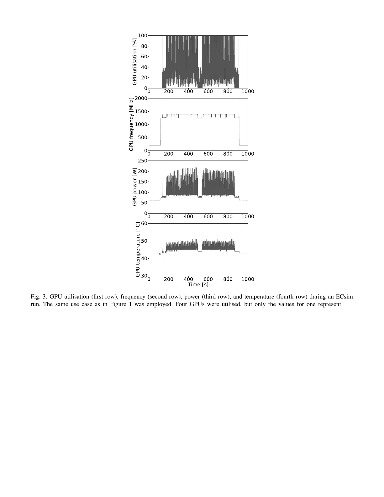
Accelerating the P article-In-Cell code ECsim with OpenA CC Elisabetta Boella ∗ ¶ , Nitin Shukla † ∥ , Filippo Spiga ‡ , Mozhgan Kabiri Chimeh ‡ , Matt Bettencourt ‡ , Maria Elena Innocenti § ∗ E4 Computer Engineering SpA , Scandiano, Italy † CINECA , Casalecchio di Reno, Italy ‡ NVIDIA Corporation , Santa Clara, United States § Ruhr-Univer sit ¨ at , Bochum, Germany ¶ elisabetta.boella@e4company .com , ∥ n.shukla@cineca.it ©2026 IEEE. Personal use of this material is permitted. Permission from IEEE must be obtained for all other uses, including reprinting/republishing this material for advertising or promotional purposes, collecting new collected works for resale or redistribution to servers or lists, or reuse of any copyrighted component of this work in other works. Abstract The Particle-In-Cell (PIC) method is a computational technique widely used in plasma physics to model plasmas at the kinetic le vel. In this work, we present our effort to prepare the semi-implicit energy-conserving PIC code ECsim for exascale architectures. T o achiev e this, we adopted a pragma-based acceleration strategy using OpenA CC, which enables high performance while requiring minimal code restructuring. On the pre-exascale Leonardo system, the accelerated code achiev es a 5 × speedup and a 3 × reduction in energy consumption compared to the CPU reference code. Performance comparisons across multiple NVIDIA GPU generations show substantial benefits from the GH200 unified memory architecture. Finally , strong and weak scaling tests on Leonardo demonstrate efficienc y of 70% and 78% up to 64 and 1024 GPUs, respectiv ely . Index T erms Particle-In-Cell, Plasma Physics, GPU acceleration, OpenACC, performance optimisation, energy efficiency . I . I N T RO D U C T I O N The Particle-In-Cell (PIC) method is a specialised particle-mesh technique widely used in plasma physics to model kinetic effects and complex plasma interactions. It combines Lagrangian and Eulerian approaches to accurately capture plasma microphysics. Specifically , plasmas are represented through a statistical distribution of charged particles, with computational macroparticles sampling the behavior of positiv e and negati ve charges. These macroparticles interact via the electromagnetic fields they generate, which are computed by solving Maxwell’ s equations on a fixed grid. The charge and current densities required for field calculations are obtained by interpolating the discrete particle properties onto the grid. In turn, the fields are used to update the position and velocity of the macroparticles [1], [2], [3]. T ypically in the PIC algorithm, Maxwell’ s and motion equations are solved utilising explicit time discretisation in a staggered fashion, with particles assumed to be frozen when updating the electromagnetic field and fields considered static when pushing particles [4]. This methodology introduces a series of stability constraints which require that the smallest scale inv olved in the problem is resolved. As a consequence, using these algorithms for modelling multiscale plasma scenarios becomes very challenging even considering the large amount of computational resources a vailable today . On the other hand, a fully implicit approach with particle and field information updated together by employing non-linear iterativ e schemes would relax the conditions for stability . Howe ver , the higher complexity of the algorithm, which requires the solution of a set of non- linearly coupled equations, increases its computational cost and could lead to conv ergence issues, thus making this solution impractical [5]. A good compromise is represented by semi-implicit PIC schemes. This type of algorithm maintains the benefits of an implicit discretisation of the relev ant equations in time and the coupling between fields and particles is retained, though in an approximate form through linearisation. As a consequence, numerical limitations typical of the explicit method are relaxed and the absence of non-linear iterations reduces the computational cost per time step of the fully implicit PIC algorithm [4], [6], [7], [8]. Thanks to these features, the semi-implicit PIC algorithm has been used over the years to successfully model the coupling between small and large scales in magnetic reconnection [9], [10], turbulence [11], instabilities [12], and plasma confinement for fusion energy [13]. Previously , we hav e implemented the semi-implicit PIC algorithm called the energy conserving semi-implicit method [14], [15] in the massively parallel code ECsim [7], [16]. The peculiarity of the scheme and the code is that both conserve energy down to machine precision contrarily to other semi-implicit schemes, such as the implicit moment method [17] or the direct implicit method [18]. This eliminates the artificial numerical cooling typical of these algorithms, which is usually controlled in simulations by selecting sufficiently small spatial and temporal steps, thus practically increasing the computational cost of simulations. In this sense, ECsim represents a step forward tow ards real multiscale plasma simulations. The code is written in C/C++ and parallelised with the Message Passing Interface (MPI 1 ) paradigm. A MPI cartesian topology is used to split the physical domain among the processes. Each process handles the field and particles on its subdomain. The code utilises the parallel libraries HDF5 2 to perform data I/O and it is built using CMake 3 . A version of the code implementing OpenMP 4 shared memory parallelism on top of MPI also exists. In this work, we describe our effort to prepare ECsim for exascale supercomputers. Normally , heterogeneity is a key characteristics of these machines, with computing nodes being equipped with accelerators, typically Graphical Processing Units (GPUs). T o tackle this challenge and exploit the high lev el parallelism offered by these devices, we decided to adopt a directive-based approach using OpenA CC 5 . OpenACC allowed us to maintain the original structure of the code without introducing intrusive changes and, at the same time, reaching good performance. It could be argued that this choice currently penalises us in terms of portability and that we could achiev e the same results by using the OpenMP offloading model. Howe ver , based on our kno wledge, at this stage OpenA CC appears to be more stable and mature with respect to OpenMP offloading and with more support from a compiler perspectiv e, thus guaranteeing better performance giv en the same effort [19]. Furthermore two out of three European pre-exascale machines are equipped with NVIDIA GPUs and the first European exascale supercomputer , Jupiter 6 (J ¨ ulich Supercomputing Centre, Germany), features NVIDIA GPUs. ECsim will be able to take full advantage of all these resources. Thus, the main contributions of this paper are: • W e accelerated the semi-implicit PIC code ECsim using OpenA CC, requiring only minimal modifications to the original code base; • W e validated the accelerated implementation against the reference CPU version and carried out performance benchmarks in terms of both time-to-solution and energy-to-solution; • W e compared the execution time of the accelerated kernels across different NVIDIA GPU models and analysed the scaling behaviour of the accelerated ECsim on the pre-exascale system Leonardo (CINECA, Italy) [20]. The paper is organised as follows. Section II overvie ws the ECsim algorithm. Section III outlines the strategy adopted to introduce GPU support in the code, reports the validation tests performed to ensure correctness, and discusses performance benchmarks comparing the accelerated implementation with the reference CPU version. Experiments on different GPU archi- tectures and scaling tests on the Leonardo supercomputer are presented in Section IV. Finally , Section V summarises the main findings and concludes the paper . I I . C O D E S T RU C T U R E Three main blocks form the core of the code: 1) moment gathering, 2) field solver , and 3) particle mov er . In the moment gathering, particle information is deposited on the grid to compute the current and the so-called mass matrices [21] later needed by the field solver . In particular , the hatted current ˆ J for each plasma species s is calculated according to the formula: ˆ J sN = 1 V N X p q p ˆ v p W pN . (1) In Equation (1), N denotes the set of closest grid nodes to which each particle contributes, with each particle influencing two nodes in each spatial direction (8 nodes in total), V N is the control volume of the node N , W pN the linear interpolation function between the particle p of species s and the node N , q p the charge of the particle p , and ˆ v p = α n p · v n p the particle velocity v n p rotated by the matrix α n p , both ev aluated at time n . The three-by-three rotation matrix is giv en by: α n p = 1 1 + ( β p B n p ) 2  I − β p I × B n p + β 2 p B n p B n p  , (2) where I is the identity matrix, B n p the magnetic field at the position of the particle p at time n , β p = q p ∆ t/ (2 m p ) , m p the mass of the particle, and ∆ t the temporal step chosen to discretise time in the simulation. The calculation of the three-by-three mass matrix is more elaborated. Each ij component can be found as: M ij N N ′ = X s X p β p V N q p α ij,n p W pN ′ W pN , (3) 1 MPI: https://www .mpi- forum.org/, accessed November 2025. 2 HDF5: https://www .hdfgroup.org/solutions/hdf5/, accessed November 2025. 3 CMake: https://cmake.org/, accessed November 2025. 4 OpenMP: https://www .openmp.org/, accessed November 2025. 5 OpenA CC: https://www .openacc.org/, accessed November 2025. 6 Jupiter: https://www .fz- juelich.de/en/jsc/jupiter, accessed November 2025. where N ′ indicates the neighbouring nodes to each node N . For each node N , 27 N ′ can be identified (see Figure 2 in [7]) and therefore 27 mass matrices should be calculated. Due to symmetry , M N N ′ = M N ′ N , only 14 mass matrices must be computed and stored in memory in practice. In the field solver , Faraday and Amp ` ere’ s equations are solved to calculate the electric and magnetic fields at the next time step. The equations are discretised in time according to the θ scheme [17] and in space employing the technique used in the code iPIC3D [22], [23]: 1 cθ ∆ t B n + θ C + ∇ C × E n + θ N = 1 cθ ∆ t B n C , (4) − 1 cθ ∆ t E n + θ N + ∇ N × B n + θ C − 4 π c X N ′ M N N ′ E n + θ p = = − 1 cθ ∆ t E n N + 4 π c ˆ J N . (5) Here, c is the speed of light in vacuum, ˆ J N is obtained by summing ˆ J sN ov er all plasma species s , and the subscript C denotes quantities e valuated at the cell centres, as opposed to those e valuated at the grid nodes N . The operator ∇ is discretised using finite difference. Usually , θ = 1 / 2 is employed; this ensures energy conservation. The system composed of Equations (4) and (5) is solved to find E n + θ and B n + θ in an iterative way . The generalised minimal residual (GMRES) method available through the PETSc library 7 is utilised. Using E n + θ and B n + θ , the electric and magnetic field values at time n + 1 are computed as E n +1 = ( θ − 1) /θ E n + 1 /θ E n + θ and B n +1 = ( θ − 1) /θ B n + 1 /θ B n + θ . The electric field at the iteration n + θ and the magnetic field at iteration n are then used in the particle mover to update each particle velocity and position prior to interpolation from the grid point to the particle. The particle pusher is designed combining the DIM D1 [24] and the theta [17] schemes. First, the particle velocity at n + 1 is computed according to the following steps: ¯ v p = α n p · v n p + β p α n p · E n + θ p ( x n − 1 / 2 p ) , (6) v n +1 p = 2 ¯ v p − v n p , (7) and, finally , the particle is moved to a new position: x n +1 / 2 = x n − 1 / 2 + ∆ t v n +1 . (8) By choosing θ = 1 / 2 , the particle mover is second order accurate in time and energy conservation is ensured [14]. These three steps are then repeated at each new time iteration. I I I . S T R A T E G Y F O R A D D I N G G P U S U P P O RT As a first step tow ard accelerating ECsim, we profiled the original CPU version of ECsim on the Booster partition of the Leonardo supercomputer; this serves as the reference implementation for the rest of the text. Each compute node in this system is equipped with an Intel Xeon Platinum 8358 CPU (codename: Ice Lake), providing 32 physical cores per node, and four NVIDIA A100 GPUs, which remained idle during the CPU tests [20]. This reference version was compiled with the NVIDIA HPC SDK 23.11 8 suite of compilers, Open MPI 4.1.6 9 , HDF5 1.14.3, OpenBLAS 0.3.24 10 , PETSc 3.20.1, and H5HUT 2.0.0 11 with -O3 flag. Figure 1 shows the result of this ex ercise for a two-dimensional simulation of the current filamentation instability [25] using a grid of 256 × 128 cells, 4 plasma species, and 60 × 60 particles per cell per species, for a total of ≈ 4 . 72 × 10 8 particles pushed for 100 time steps. The high number of computational particles is required to decrease the numerical noise and improve the correctness and accuracy of the results [2] and is a crucial parameter in ECsim, which relies solely on linear interpolation and does not implement spatial smoothing, as the latter would compromise energy conservation. W e note that a recent work has proposed a smoothing technique that preserves energy conservation [26]; howe ver , this approach is not used in our current implementation of ECsim. The simulation was performed using 32 MPI tasks equi valent to a full node. W e observe that, although the grid is slightly smaller than what is typically used in production runs, the workload per core remains representative of production conditions. The number of I/O operations also closely matches that of a standard production run. As shown by Figure 1, most of the time is spent by the code in the moment gathering portion ( ≈ 76% of the total simulation time). This is followed by I/O and the particle mover . The I/O part accounts not only for writing to disk operations, but also for 7 PETSc: https://petsc.org/release/, accessed November 2025. 8 NVIDIA HPC SDK 23.11: https://dev eloper .n vidia.com/n vidia- hpc- sdk- 2311- downloads, accessed November 2025 9 Open MPI 4.1.6: https://www .open- mpi.org/software/ompi/v4.1/, accessed November 2025. 10 OpenBLAS: http://www .openmathlib .org/OpenBLAS/, accessed November 2025. 11 H5HUT : https://gitea.psi.ch/h5hut new/src, accessed November 2025. CPU GPU 0 1000 2000 3000 4000 Walltime [s] 1.0x 5.0x Fig. 1: W alltime and speedup for a typical 2D simulation using the CPU reference (left bar) and OpenACC-accelerated (right bar) ECsim on one node of Leonardo Booster . Colours denote code sections: blue initialisation, orange moment gathering, green field solver , purple particle mover , and gray I/O. The pure CPU simulation was ran with 32 MPI ranks, the heterogeneous simulation was performed with four GPUs and four MPI tasks. the calculation of quantities such as plasma density , current, pressure, and heat flux, necessary for diagnostic purposes rather than for temporal ev olution. These computations basically entail interpolating particle to the grid. Initialisation and field solver last a negligible time with respect to the rest of the code. Thus the CPU profiling provides a clear indication of the kernels for which GPU offloading could be the most beneficial: particle mover , moment gathering, and diagnostics calculations in the I/O. Our primary focus of this work is indeed accelerating these kernels to enhance performance of ECsim, by reducing the ov erall time-to-solution. W e started by accelerating the particle mo ver , which is composed of three main functions: updataVelocity , updatePosition , and fixPosition . In the first two functions the velocity of each particle at t n +1 and their position at t n +1 / 2 are computed, respectiv ely , employing Equations (7) and (8), which use previously stored values of the electric and magnetic fields at the position of the particles. The third function is only called if the simulation is one or two-dimensional and set the particle position along the same line or on the same plane. This step is necessary to ensure the correctness of the mass matrix calculations in case of reduced simulation dimensions. The underlying structure of all these functions is similar , as each of them contains a for loop ov er all particles. Since the com- putations exhibit no data dependencies, acceleration was achiev ed simply by adding the #pragma acc parallel loop directiv e before the loops. As a first step, we allowed the compiler to manage memory transfers automatically and therefore did not include any explicit clauses for moving data between the host and the device. The updateVelocity function makes use of the field information, which was stored as three-dimensional pointers of size N x × N y × N z , where N x , N y , and N z represent the number of grid points per MPI rank along the x , y , and z directions, respectiv ely . Before introducing the OpenACC pragmas, these three-dimensional pointers were flattened into one-dimensional arrays to improve data locality and assist the compiler in optimisation. W e then tackled the moment gathering. The core routine in this case is computeMoments , where ˆ J sN and M ij N N ′ are computed. Each component of the hatted current ( ˆ J sN ,x , ˆ J sN ,y , ˆ J sN ,z ) is represented in memory as a four-dimensional array of size N s × N x × N y × N z with N s indicating the number of plasma species considered. The nine components of the mass matrix, i.e. M xx N N ′ , M xy N N ′ , M xz N N ′ , M y x N N ′ , M y y N N ′ , M y z N N ′ , M z x N N ′ , M z y N N ′ , M z z N N ′ , are each also stored in a four-dimensional array with size 14 × N x × N y × N z with no distinction between plasma species. As described in Section II, for each node N , 14 mass matrices must be computed. The function computeMoments contains a for loop ov er all particles. W ithin this loop, the grid node with the highest index to which each particle contributes is first identified in e very spatial direction. Because linear interpolation is used, each particle interacts with two grid points per direction, denoted N − and N + . Once N + is kno wn, the corresponding lower index N − is simply obtained by subtracting one. Overall, this yields 2 3 = 8 grid points that receiv e contributions from a single particle. The interpolation weights mapping the particle position to these surrounding nodes, W pN , are then computed and stored in a 2 × 2 × 2 weight array . The weight array is used within the for loop over the particles to calculate the value of the magnetic field at each particle position. Originally this was done through three nested mini-loops along the dimensions of the grid with index being either 0 or 1 and mapping to either N − or N + in each direction. These loops were manually unrolled to exploit parallelism and improv e memory coalescing on the GPU, thereby reducing loop overhead and increasing computational throughput. T o aid with this both the weight and magnetic field three-dimensional arrays were flattened. After computing the v alue of the magnetic field at the particle position, a rotation matrix is computed for each particle. In the reference CPU code, the rotation matrix is stored in a 3 × 3 array with elements α ij . Here, with the intent of improving data locality , we eliminated the bi-dimensional array and defined nine scalars, one for each element of the original matrix. The current ˆ J sN is then computed by summing the contribution of each particle, namely q p α n p · v n p , to the neighbouring grid points. In the original CPU version of the code this was done component by component ( ˆ J sN ,x , ˆ J sN ,y , ˆ J sN ,z ) through again three nested mini-loops along the dimension of the grid with index being either 0 or 1. For the same reasons listed above, we decided to unroll manually these mini-loops. The routine proceeds by computing the 14 mass matrices, each with nine components. In this case we made only minimal changes to the instructions used in the CPU code. Originally the computation of the mass matrix components in volv ed six nested loops: three loops over the spatial dimensions with indexes varying between 0 and 1 to identify the closest nodes to the particle in each direction, one loop from 0 to 14 for the neighbour nodes N ′ , and finally two loops to ef fectiv ely compute the contribution of p to the three-by-three ( i, j ) component of each mass matrix. These latter values were then accumulated to M N N ′ , with if conditions used to select the nodes to which each particle has to accumulate. First, we observed that the access pattern to the four-dimensional arrays storing the mass matrices was suboptimal in terms of memory locality . Consequently , we modified the access order to maintain the leftmost dimension (loop over N ′ ) as the outermost loop. This implied some further modifications. W e introduced a switch construct to identify the correct neighbour to the node N among the 14 possibilities. W e maintained three for mini-loops ov er the grid dimensions with index es varying between 0 and 1. This, together with if conditions to exclude nodes too far from the particle, allowed us to identify both the relev ant nodes and the amount to deposit there, e.g. q p β α ij W pN ′ W pN . The overall four for loops serve to sum also the different contributions to the nine components of each mass matrix. T o accelerate computeMoments , after the modifications we hav e mentioned, we added the directi ve #pragma acc parallel loop before the for loop over the particles. Additionally , to av oid race conditions caused by concurrent threads accessing the same memory location, we had to resort to #pragma acc atomic update before summing the contributions for ˆ J sN and M ij N N ′ . W e remark that the routine still contains three relatively small inner loops. Full loop unrolling was not applied, as it would increase register pressure and consequently degrade ex ecution performance. Diagnostics for I/O are computed through two routines, computeCharge and computeCurrent , which ev aluate the charge density , charge current, and pressure tensor . The diagnostic charge current differs from ˆ J , as it excludes the effect of velocity rotation. The structure of these routines closely resembles that of computeMoments : each contains a for loop ov er the particles and a summation that accumulates their individual contributions. T o accelerate these computations, the loops were parallelised using #pragma acc parallel loop , and the summations were made thread-safe through the use of #pragma acc atomic update . W e note that the use of #pragma acc atomic update could potentially be avoided by sorting the particles and employing a reduction clause for the summation. Howe ver , when we attempted to implement this approach, compiler limitations arose with array based reductions, and we decided not to pursue this approach further . Performance analysis using NVIDIA Nsight Systems re vealed substantial data transfers between the host and device, accompanied by numerous page faults during GPU kernel execution. T o address this, we chose to continue using managed memory while lev eraging the CUD A memory management function cudaMemPrefetchAsync to efficiently manage data migration between the host and device. Specifically , cudaMemPrefetchAsync(x, sizeof(double) * n, 0, 0) was used to transfer an array x of n double elements to the GPU before its use, while cudaMemPrefetchAsync(x, sizeof(double) * n, cudaCpuDeviceId, 0) was employed to migrate the same array back from the device to the host. This approach improves performance while circumventing the intricate issues associated with deep-copying complex data structures. Before e valuating the performance of the accelerated code, we first validated its accuracy by comparing the results against those obtained with the CPU reference version. Specifically , we performed simulations on the Leonardo Booster partition of well-known one- and two-dimensional plasma instabilities using both code variants. The accelerated ECsim was compiled with the same software stack as the reference version, but with the following additional compiler flags: -cuda -acc -gpu=cc80,managed,lineinfo,cuda12.3 -Minfo=accel , along with -O3 for optimisation. Both one- and two- dimensional simulations were ex ecuted using four MPI tasks on the CPU, and four MPI tasks, each bound to a distinct NVIDIA A100 GPU, when running with accelerator support. The Open MPI flags --bind-to core and --map-by ppr:4:node:PE=8 were used in both cases. Figure 2 shows the temporal ev olution of the electric and magnetic field energies for the two- stream instability [27] (left panel) and the current-filamentation instability [25] (right right), standard reference cases for electrostatic and electromagnetic dynamics, respectiv ely . The results display the characteristic exponential growth typical of these phenomena. The curves produced by the GPU-accelerated version of ECsim overlap perfectly with those from the reference implementation, confirming the correctness and numerical consistency of the accelerated code. Once the correctness of the code had been established, we measured its performance by repeating the same simulation shown in Figure 1 using the four GPUs av ailable on a node of the Booster partition of Leonardo each associated to one MPI rank. For the performance ev aluation, a full node was allocated exclusi vely . The same Open MPI flags and GPU binding techniques used for Figure 2 were employed. Execution times are reported in Figure 1. The GPU-accelerated version of the code completed 0 20 40 60 T ime [ 1 ] 10 6 10 4 Energy [m i c 2 ] 0 5 10 15 T ime [ 1 ] 10 8 10 7 10 6 10 5 Energy [m i c 2 ] Fig. 2: T ime evolution of the electric field energy (left panel) and magnetic field energy (right panel) from simulations of the two-stream instability (left panel) and current filamentation instability (right panel), respectiv ely . Red solid lines show results from the CPU reference version of ECsim, while black dashed lines correspond to the accelerated version of the code. All values are normalised to reference quantities. the simulation in ≈ 787 s , achieving an overall speedup of 5 × relati ve to the reference CPU implementation, which utilised all the 32 cores available on one node. The moment-gathering block now accounts for only 23% of the ex ecution time, with a duration comparable to the other code blocks. W e note that this overall 5 × speedup was achieved with partial offloading of the code. Functions that remain on the CPU and are parallelised solely via MPI, such as initialisation and field calculation, are approximately eight times slower in our experiment due to the lower number of MPI tasks (four vs 32) used in the offloaded version. In contrast, the moment gathering block is accelerated by a factor of 15 × , while the field solver and I/O routines are roughly twice as fast. Using the NVIDIA System Management Interface ( nvidia-smi ), we monitored the behaviour of the four GPUs available on a Leonardo Booster node during a series of ten simulations based on the run shown in Figure 1. In particular , nvidia-smi was run in the background in user space throughout each simulation, and its output was logged to a text file at a frequency of ≈ 1 Hz , following the methodology in [28], [29]. Figure 3 shows the time e volution of the GPU utilisation fraction, streaming multiprocessor (SM) frequency , power , and temperature for one of the four GPUs during a representative run. The other GPUs, not shown here, exhibit the same behaviour , and these trends are consistently observed across all ten simulations. Each simulation was preceded and followed by an interval of 120 s sleep to ensure that the GPUs returned to idle conditions between consecutiv e runs. During these periods, GPU utilisation remained at 0 , and the clock frequency , power , and temperature stabilised at idle values, namely , a frequency of 210 MHz , a po wer consumption of ≈ 60 W , and a temperature oscillating between 42 and 43 ◦ C . The beginning and end of the ECsim simulation are indicated by vertical black lines in the figure. At the start of the simulation, a short initialisation phase lasting less than 2 s occurs, during which the GPU remains in an idle state. Immediately afterwards, results at t = 0 are dumped to disk. This operation produces a peak in GPU utilisation and in all related parameters because, as discussed in Section III, the calculations of plasma density , current, and pressure are performed on the GPU. During the subsequent write-to-disk phase, GPU metrics exhibit a local minimum, although still above idle levels. This I/O step is longer than usual because RA W particle data are sav ed at this point; giv en the number of particles and despite parallelisation, this operation requires ≈ 50 s . While grid data are sav ed at every cycle and require only a few seconds, RA W particle data are sav ed three times during the simulation, and these ev ents are clearly recognisable in Figure 3. During these heavy I/O operations, only the CPU is activ e; consequently , GPU-related parameters temporarily drop to local minima. Outside these I/O phases, GPU utilisation oscillates between 100% , when GPU kernels are executed, and very low values when the time step enters code sections that are not offloaded. Con versely , the SM clock frequency shows limited variation. Except during the particle dump to disk, it remains at 1395 MHz , slightly belo w the maximum frequency of 1410 MHz . GPU power and temperature follow the utilisation pattern, reaching peaks of ≈ 210 W and ≈ 50 ◦ C , respectively . From these measurements several considerations can be drawn. First, the GPU is efficiently saturated during the phases where kernels are launched, as indicated by utilisation spikes to 100% and the corresponding increases in power and temperature. Second, the long plateaus at low utilisation highlight that the overall performance is partially constrained by CPU-side work and, in particular , by I/O. The pronounced local minima during RA W particle dumps indicate that the GPU remains mostly idle during heavy disk operations. Finally , the nearly constant SM frequency during compute phases indicates that the GPU operates close to its intended performance en velope, without significant thermal throttling or po wer capping. This confirms that the observed performance fluctuations are driv en by algorithmic and I/O patterns rather than hardware limitations. W ith the goal of understanding the energy consumption of a typical simulation, we also monitored the energy absorbed by the CPU. T o obtain meaningful statistics, we launched ten simulations with the reference CPU-only code using 32 MPI tasks and ten simulations with the accelerated code using 4 MPI tasks and 4 GPUs. Simulations were not constrained to the same 0 200 400 600 800 1000 0 20 40 60 80 100 GPU utilisation [%] 0 200 400 600 800 1000 0 500 1000 1500 2000 GPU fr equency [MHz] 0 200 400 600 800 1000 0 50 100 150 200 250 GPU power [W] 0 200 400 600 800 1000 T ime [s] 30 40 50 60 GPU temperatur e [°C] Fig. 3: GPU utilisation (first row), frequency (second ro w), power (third row), and temperature (fourth row) during an ECsim run. The same use case as in Figure 1 was employed. Four GPUs were utilised, but only the values for one representative device are shown here due to the strong similarity across all GPUs. physical node, so results reflect a representati ve sample across multiple nodes. The physical problem solved corresponds to the same use case shown in Figure 1. CPU energy consumption was measured using perf stat -a -e in combination with a one-second sleep interval. On Leonardo Booster , unlike on other supercomputers, this command does not require sudo privile ges and can therefore be used directly in user space. As with GPU po wer measurements, CPU energy samples were collected in the background while the simulations were running and output to a text file. W e note that this analysis focuses solely on CPU and GPU; energy contributions from RAM, disks, network, and other node components are neglected. Starting from the po wer measurements, the energy-to-solution for each NVIDIA A100 GPU was computed by performing a discrete integration of the recorded power samples over the simulation time (excluding the sleep intervals). The total accelerator energy was then obtained by summing the contributions from all four GPUs. The processor energy was computed analogously by summing ov er v alues collected with perf , again considering only the simulation time. The total energy-to-solution of a single run was therefore obtained as the sum of CPU and GPU contributions. Figure 4 shows the distributions of total energy for the ten CPU-only simulations (left panel) and the ten CPU+GPU simulations (right panel). On average, the reference CPU code required 1294 . 74 ± 16 . 72 kJ , whereas the accelerated code consumed 415 . 33 ± 5 . 55 kJ , demonstrating a ≈ 3 × improvement in energy efficiency . The absolute reduction in energy consumption stems from two complementary effects: the accelerated code both reduces time-to-solution and shifts the bulk of the computation to GPUs, which offer significantly higher performance per watt compared to CPUs for these kernels. Howe ver , the CPU contribution in the accelerated runs remains non-negligible, 400 800 1200 Energy-to-solution [kJ] 0.00 0.01 0.02 0.03 0.04 # sim [arb.un.] 400 800 1200 Energy-to-solution [kJ] 0.00 0.01 0.02 0.03 0.04 # sim [arb.un.] Fig. 4: Distribution of energy values across ten simulations for runs on CPU only (left panel) and on GPU (right panel). The red dashed lines represent the average energy-to-solution. Same input parameters and number of MPI tasks and GPUs as in Figure 1 were used. reflecting the fact that ECsim still performs significant CPU-side operations, including I/O, domain decomposition updates, and other tasks not offloaded to the GPU. The ratio between CPU and GPU energy suggests that further optimisations, such as optimising heavy I/O phases, improving CPU–GPU ov erlap, or offloading additional routines, could yield even larger energy savings. I V . P E R F O R M A N C E E V A L UATI O N W e compared the performance of the GPU-enabled ECsim on different generation of NVIDIA GPUs. In particular we compared V100, A100, H100, and GH200. For completness, we report here also the type of hosting system in the case of the first three accelerators: IBM Power 9, Intel Cascade Lake, and AMD Genoa. For this comparison, we performed simulations using a two-dimensional grid with 128 × 128 cells, each containing 6400 computational particles. The simulations comprised 596 temporal iterations. All the simulations were performed using 1 MPI task and 1 GPU. Results are reported in Figure 5, sho wing the execution time of the particle mover (left panel) and moment gathering (right panel) across different NVIDIA GPU generations. In both cases, execution time decreases as newer GPUs are employed. For the particle mov er , we observe a modest speedup of about 1 . 4 × on both A100 and H100 compared to V100, which exhibits the slowest performance. Kernels in the particle mover are primarily memory-bound. Their performance depends more on memory latency and bandwidth than on the av ailable compute capability . Both A100 and H100 feature similar memory- bandwidth scaling for global memory operations when accessed through OpenA CC-managed loops, explaining the limited improv ement between them. On GH200, ho wev er , the particle mover runs about twice as fast as on the V100. This gain can be attributed to the unified CPU–GPU memory architecture of the GH200, where CPU and GPU share the same physical memory pool via NVLink-C2C interconnect. In this configuration, the prefetch operations ef fectiv ely become low-o verhead cache hints rather than explicit host–de vice transfers, eliminating PCIe data mov ement costs. As a result, memory accesses are more uniform and latency is significantly reduced. The moment gathering kernel shows a much stronger performance improvement. Speedups relativ e to V100 reach 3 . 76 × , 8 . 4 × , and 12 . 79 × on A100, H100, and GH200, respectiv ely . This behaviour can be explained by a combination of factors. Newer GPUs have larger memory bandwidth, which directly benefits a memory-bound kernel like this one. Both A100 and especially H100 implement more efficient atomic instructions at the hardware level, drastically reducing contention and serialisation penalties during accumulation operations. They are equipped with larger and more efficient L2 caches, which help coalesce and buf fer atomic writes, mitigating contention. Finally , as with the particle mov er , GH200 shared memory eliminates the need for costly data migration, further boosting performance. Finally , in both cases, the CUDA driv er may also hav e contributed to the performance improv ements, as more recent CUDA versions (av ailable on newer systems) provide better optimisation of OpenA CC-generated kernels. W e performed strong and weak scaling tests of the accelerated version of ECsim on the Booster partition of Leonardo. In these tests, the dynamics of a warm plasma were modelled. In such simulations, particles move between nodes and place stress on memory access, making them representativ e of typical production runs. For the strong scaling tests, three sets of simulations were carried out using grids of 840 × 840 , 3360 × 1680 , and 6720 × 6720 cells, starting with 4 , 32 , and 256 GPUs, respectiv ely . All simulations used approximately 3000 particles per cell and 100 time steps. Results are reported in T able I and shown graphically in Figure 6, which displays the speedup (top panel) and the efficienc y (bottom panel). These tests demonstrate that ECsim achie ves near-ideal speedup for GPU counts up to 64. For larger numbers of GPUs, the parallel efficienc y gradually decreases, likely as a consequence of increased communication overhead and memory access costs. A similar behaviour has been observed for the iPIC3D code [22], whose underlying MPI parallelisation V100 Power 9 A100 C. Lake H100 Genoa GH200 0 500 1000 W alltime [s] 1.0x 1.43x 1.4x 2.09x V100 Power 9 A100 C. Lake H100 Genoa GH200 0 2000 4000 6000 W alltime [s] 1.0x 3.76x 8.4x 12.79x Fig. 5: W alltime results for the particle mover (left panel) and moment gathering (right panel) obtained on various NVIDIA GPU generations. The corresponding CPU configurations are provided for completeness. Speedup values sho wn above the bars are computed relative to the walltime obtained on the V100 GPU. Nodes GPUs W alltime [s] Speedup Efficiency [%] 1 4 2421.48 1.00 100.00 2 8 1165.74 2.08 103.86 4 16 611.30 3.96 99.03 8 32 371.50 6.52 81.48 16 64 215.02 11.26 70.38 32 128 165.32 14.65 45.77 8 32 2732.51 8.00 100.00 16 64 1323.41 16.52 103.24 32 128 710.40 30.77 96.16 64 256 419.65 52.09 81.39 128 512 282.80 77.30 60.39 64 256 2978.46 64.00 100.00 128 512 1478.11 128.96 100.75 256 1024 896.22 212.70 83.08 T ABLE I: Strong scaling results for three problem sizes: 840 × 840 (top table), 3360 × 1680 (middle table), and 6720 × 6720 (bottom table) cells. is closely related to that of ECsim. Indeed, as shown in [30], [31], the time spent in MPI communications and the associated latency increase with the number of processes, causing a significant degradation of transfer efficienc y when simulations employ a large number of cores. Although this analysis refers to a pure MPI implementation, the introduction of GPU acceleration can further amplify these effects, since faster on-device computations increase the relativ e impact of inter-process communication. In order to maintain a parallel efficienc y above 70% for 64 GPUs and beyond, it was therefore necessary to increase the grid size. With these larger grid, we observed quasi-linear speedup from 32 to 256 GPUs, with a measured parallel ef ficiency of 81% , after which an even larger problem size had to be considered. In the final set of simulations with a grid of 6720 × 6720 cells, starting from 256 GPUs, we achieved a parallel ef ficiency of 83% at 1024 GPUs, confirming that ECsim can sustain high performance even at large scale. In the weak scaling tests, we started with simulations using four GPUs on a single Leonardo Booster node with a grid of 128 × 128 cells. The grid was then progressiv ely increased up to 2048 × 2048 cells, utilising 256 Leonardo Booster nodes (1024 GPUs), which corresponds to the maximum number of nodes a single user can request on this system. Each simulation employed 200 × 200 particles per cell per species for a total of four plasma species, and 100 temporal steps were executed. T able II and Figure 7 present the results, demonstrating that ECsim exhibits excellent weak scaling. As the number of GPUs increases, the runtime remains nearly constant, indicating that communication and memory overheads grow moderately e ven at large scale. The measured parallel ef ficiency remains abov e 78 . 13% for 1024 GPUs, corresponding to a speedup that closely follows the ideal linear trend for weak scaling. These results confirm that ECsim can ef fectiv ely utilise large numbers of GPUs while maintaining high computational performance, making it suitable for large-scale plasma simulations where particle motion between nodes can stress memory access and communication patterns. V . S U M M A RY & P E R S P E C T I V E S In this work, we describe our strategy for offloading the most computationally intensive kernels of the PIC code ECsim using OpenACC directiv es, which allows us to maximize performance without requiring extensiv e code restructuring. Our performance ev aluation, in terms of both time-to-solution and energy-to-solution, using a node-to-node comparison on the Leonardo Booster partition, shows that the accelerated code achie ves 5 × faster execution and 3 × higher energy efficiency compared to the CPU version. 4 8 16 32 64 128 256 512 1024 GPUs 1 0 0 1 0 1 1 0 2 Speedup 1 2 4 8 16 32 64 128 256 Nodes 0 25 50 75 100 Efficiency 840x840 3360x1680 6720x6720 Fig. 6: Parallel speedup (top panel) and efficiency (bottom panel) from strong scaling tests on the Leonardo Booster partition for problem sizes of 840 × 840 (blue), 3360 × 1680 (orange), and 6720 × 6720 (green) cells. Black lines indicate the ideal values. Nodes GPUs W alltime [s] Speedup Efficiency [%] 1 4 2416.41 1.00 100.00 2 8 2450.68 1.97 98.60 4 16 2463.25 3.92 98.10 8 32 2490.84 7.76 97.01 16 64 2501.75 15.45 96.59 32 128 2538.33 30.46 95.20 64 256 2805.62 55.12 86.13 128 512 2880.18 107.39 83.90 256 1024 3092.61 200.03 78.13 T ABLE II: W eak scaling results. W e further ev aluated the performance of the ported kernels across multiple generations of NVIDIA GPUs. The results show that they benefit significantly from the unified memory av ailable on the GH200 Superchip, while the larger memory bandwidths of newer GPUs contribute substantially to the acceleration of memory-bound kernels in ECsim. Additionally , a kernel that relies heavily on atomic operations experiences notable speedup thanks to the more efficient hardware implementation of these instructions in modern GPU architectures. Furthermore, we demonstrate that ECsim scales ef fectiv ely across multiple GPUs. In strong scaling tests, the code achie ves a parallel efficiency of 70% up to 64 GPUs (16 nodes), while in weak scaling tests it maintains a parallel efficienc y of 78% up to 1024 GPUs (256 nodes). Finally , we note that while comparisons with nativ e multi-GPU PIC implementations or with other highly optimised open- source PIC codes would undoubtedly enrich the discussion, such comparisons are neither straightforward nor entirely fair . ECsim is intrinsically distinct from many existing PIC codes due to the numerical scheme it employs. In contrast, many highly optimised PIC codes based on pure CUD A [32], [33], [34], K okkos [35], Alpaka [36], or SYCL [37] rely on different algorithmic choices, data layouts, and execution models, making direct comparisons based solely on raw performance metrics difficult to interpret. For this reason, the performance results presented in this work are primarily benchmarked against the original CPU implementation of ECsim, which provides a consistent and meaningful reference for assessing the impact of GPU acceleration. Comparisons with other PIC codes were previously carried out during the v alidation phase of ECsim, most notably against iPIC3D, which shares a similar MPI parallelisation strategy . These studies focused on numerical accuracy and physical fidelity , and only partially on performance. They showed that, in one-to-one comparisons, ECsim was slightly slower than iPIC3D; 4 8 16 32 64 128 256 512 1024 GPUs 1 0 0 1 0 1 1 0 2 Speedup 1 2 4 8 16 32 64 128 256 Nodes 0 25 50 75 100 Efficiency Fig. 7: Same as in Figure 6, but for weak scaling tests. howe ver , it could achie ve faster times-to-solution by e xploiting lar ger time steps and coarser spatial resolutions while maintaining the same level of accuracy [7], [16]. While native GPU implementations of ECsim based on CUD A, Kokk os, or SYCL could in principle be de veloped, such approaches would require intrusiv e refactoring and a substantial redesign of the existing production-ready code. The primary objectiv e of the present work is instead to enable efficient exploitation of GPU architectures while preserving the original code structure. T o this end, a directiv e-based OpenA CC approach was adopted, offering a practical compromise between performance, portability , and dev elopment effort. Nevertheless, as part of our ongoing work, a pure CUDA implementation of ECsim is currently under dev elopment and will provide valuable insight into the potential performance benefits of a fully nativ e GPU approach. Finally , as a future perspective, we plan to explore the use of cellular automata and high-performance libraries specifically designed for cellular automata as a means to improve performance [38], [39]. A C K N O W L E D G M E N T E.B. and N.S. contributed equally to this work. E.B. and N.S. acknowledge support from the SP ACE project, funded by the European Union. This project has receiv ed funding from the European High Performance Computing Joint Undertaking (JU) and from Belgium, the Czech Republic, France, Germany , Greece, Italy , Norway , and Spain under grant agreement No. 101093441. M.E.I. acknowledges support from the Deutsche Forschungsgemeinschaft (German Research Foundation), project numbers 497938371 and 544893192. E.B. would like to thank Daniele Gregori (E4 Computer Engineering) for fruitful discussions. This work is dedicated to the memory of Prof. Giov anni Lapenta, whose guidance and encouragement inspired this study . R E F E R E N C E S [1] J. M. Dawson, “Particle simulation of plasmas, ” Reviews of Modern Physics , vol. 55, p. 403, 1983. [2] C. K. Birsdall and A. B. Langdon, Plasma physics via computer simulation . McGraw–Hill Book Company , 1985. [3] R. Hockney and J. Eastwood, Computer simulation using particles . T aylor and Francis, 1988. [4] G. Lapenta, “Particle simulations of space weather, ” Journal of Computational Physics , vol. 231, pp. 795–821, 2012. [5] S. Markidis and G. Lapenta, “The energy conserving particle-in-cell method, ” Journal of Computational Physics , vol. 230, pp. 7037–7052, 2011. [6] G. Lapenta, S. Markidis et al. , “Space weather prediction and exascale computing, ” Computing in Science & Engineering , vol. 15, no. 5, pp. 68–76, 2013. [7] D. Gonzalez-Herrero, E. Boella, and G. Lapenta, “Performance analysis and implementation details of the Energy Conserving Semi-Implicit Method code (ECsim), ” Computer Physics Communications , vol. 229, p. 162, 2018. [8] G. Lapenta, “Particle-based simulation of plasmas, ” in Plasma Modeling (Second Edition) , ser . 2053-2563. IOP Publishing, 2022, pp. 4–1 to 4–37. [9] G. Lapenta, S. Markidis et al. , “Secondary reconnection sites in reconnection-generated flux ropes and reconnection front, ” Nature Physics , vol. 11, pp. 690–695, 2015. [10] M. E. Innocenti, M. Goldman et al. , “Evidence of magnetic field switch-off in collisionless magnetic reconnection, ” The Astrophysical Journal Letters , vol. 810, p. L19, 2015. [11] L. Franci, E. Papini et al. , “ Anisotropic electron heating in turbulence-driv en magnetic reconnection in the near-sun solar wind, ” The Astr ophysical Journal , vol. 936, no. 1, p. 27, 2022. [12] A. Micera, E. Boella et al. , “Particle-in-cell simulations of the parallel proton firehose instability influenced by the electron temperature anisotropy in solar wind conditions, ” The Astr ophysical Journal , vol. 893, no. 2, p. 130, 2020. [13] J. Park, N. A. Krall et al. , “High-energy electron confinement in a magnetic cusp configuration, ” Phys. Rev . X , vol. 5, p. 021024, Jun 2015. [14] G. Lapenta, “Exactly energy conserving semi-implicit particle in cell formulation, ” Journal of Computational Physics , vol. 334, p. 349, 2017. [15] G. Lapenta, D. Gonzalez-Herrero, and E. Boella, “Multiple-scale kinetic simulations with the energy conserving semi-implicit particle in cell method, ” Journal of Plasma Physics , vol. 83, p. 705830205, 2017. [16] D. Gonzalez-Herrero, A. Micera et al. , “Ecsim-cyl: Energy conserving semi-implicit particle in cell simulation in axially symmetric cylindrical coordinates, ” Computer Physics Communications , vol. 236, pp. 153–163, 2019. [17] J. Brackbill and D. Forslund, “ An implicit method for electromagnetic plasma simulation in two dimension, ” Journal of Computational Physics , vol. 46, p. 271, 1982. [18] A. Langdon, B. I. Cohen, and A. Friedman, “Direct implicit large time-step particle simulation of plasmas, ” Journal of Computational Physics , vol. 51, no. 1, pp. 107–138, 1983. [19] M. Stack, P . Macklin et al. , “OpenACC Acceleration of an Agent-Based Biological Simulation Framew ork, ” Computing in Science & Engineering , vol. 24, no. 05, pp. 53–63, 2022. [20] M. Turisini, G. Amati, and M. Cestari, “Leonardo: A pan-european pre-exascale supercomputer for hpc and ai applications, ” 2023. [21] D. Burgess, D. Sulsky , and J. Brackbill, “Mass matrix formulation of the flip particle-in-cell method, ” Journal of Computational Physics , vol. 103, no. 1, pp. 1–15, 1992. [22] S. Markidis, G. Lapenta, and Rizwan-uddin, “Multi-scale simulations of plasma with iPIC3D, ” Mathematics and Computers and Simulation , vol. 80, p. 1509, 2010. [23] J. J. W illiams, D. Medeiros et al. , “Characterizing the performance of the implicit massively parallel particle-in-cell ipic3d code, ” 2024. [24] D. W . Hewett and A. Bruce Langdon, “Electromagnetic direct implicit plasma simulation, ” Journal of Computational Physics , vol. 72, p. 121, 1987. [25] B. D. Fried, “Mechanism for instability of transverse plasma wav es, ” The Physics of Fluids , vol. 2, no. 3, pp. 337–337, 1959. [26] G. Lapenta, “ Advances in the implementation of the exactly energy conserving semi-implicit (ecsim) particle-in-cell method, ” Physics , vol. 5, no. 1, pp. 72–89, 2023. [27] R. Davidson, Kinetic waves and instabilities in a uniform plasma . North-Holland., 1983, vol. 1. [28] G. Amati, M. T urisini et al. , “Experience on clock rate adjustment for energy-ef ficient gpu-accelerated real-world codes, ” in High P erformance Computing: ISC High P erformance 2025 International W orkshops, Hambur g, Germany , June 10–13, 2025, Revised Selected P apers . Berlin, Heidelberg: Springer- V erlag, 2025, p. 245–257. [29] J. L. Almerol, E. Boella et al. , “ Accelerating gravitational n-body simulations using the risc-v-based tenstorrent wormhole, ” in Proceedings of the SC ’25 W orkshops of the International Conference for High P erformance Computing, Networking, Storage and Analysis , ser . SC W orkshops ’25. New Y ork, NY , USA: Association for Computing Machinery , 2025, p. 1729–1735. [30] N. Shukla, A. Romeo et al. , “Eurohpc space coe: Redesigning scalable parallel astrophysical codes for exascale. invited paper, ” in Proceedings of the 22nd A CM International Confer ence on Computing F rontier s: W orkshops and Special Sessions , ser . CF ’25 Companion. New Y ork, NY , USA: Association for Computing Machinery , 2025, p. 177–184. [31] ——, “T ow ards exascale computing for astrophysical simulation lev eraging the leonardo eurohpc system, ” Pr ocedia Computer Science , vol. 267, pp. 112–123, 2025, proceedings of the Third EuroHPC user day . [32] C. P . Sishtla, S. W . D. Chien et al. , Multi-GPU Acceleration of the iPIC3D Implicit P article-in-Cell Code . Springer International Publishing, 2019, p. 612–618. [33] S. W . D. Chien, J. Nylund et al. , “sputnipic: An implicit particle-in-cell code for multi-gpu systems, ” in 2020 IEEE 32nd International Symposium on Computer Arc hitecture and High P erformance Computing (SBAC-P AD) . IEEE, Sep. 2020, p. 149–156. [34] L. Fedeli, A. Huebl et al. , “Pushing the Frontier in the Design of Laser-Based Electron Accelerators with Groundbreaking Mesh-Refined Particle-In-Cell Simulations on Exascale-Class Supercomputers, ” in SC22: International Conference for High P erformance Computing, Networking, Storage and Analysis . Los Alamitos, CA, USA: IEEE Computer Society , Nov . 2022, pp. 1–12. [35] R. Bird, N. T an et al. , “Vpic 2.0: Next generation particle-in-cell simulations, ” IEEE T ransactions on P arallel and Distributed Systems , vol. 33, no. 4, p. 952–963, Apr . 2022. [36] M. Bussmann, H. Burau et al. , “Radiative signatures of the relativistic kelvin-helmholtz instability , ” in Pr oceedings of the International Conference on High P erformance Computing, Networking, Storage and Analysis , ser . SC ’13. New Y ork, NY , USA: ACM, 2013, pp. 5:1–5:12. [37] I. V asileska, P . T om ˇ si ˇ c et al. , “Un veiling performance insights and portability achievements between cuda and sycl for particle-in-cell codes on different gpu architectures, ” in 2024 47th MIPRO ICT and Electr onics Convention (MIPR O) , 2024, pp. 1115–1120. [38] P . Chaisiriroj and R. B. Stone, “Performance analysis of automatascales to support early design decisions, ” in Proceedings of the ASME 2024 International Design Engineering T echnical Confer ences and Computers and Information in Engineering Conference , ser . International Design Engineering T echnical Conferences and Computers and Information in Engineering Conference, vol. V olume 2A: 44th Computers and Information in Engineering Conference (CIE), 2024, p. V02A T02A042. [39] D. D’Ambrosio, A. De Rango et al. , “The open computing abstraction layer for parallel complex systems modeling on many-core systems, ” Journal of P arallel and Distributed Computing , vol. 121, pp. 53–70, 2018.