Simplex-to-Euclidean Bijection for Conjugate and Calibrated Multiclass Gaussian Process

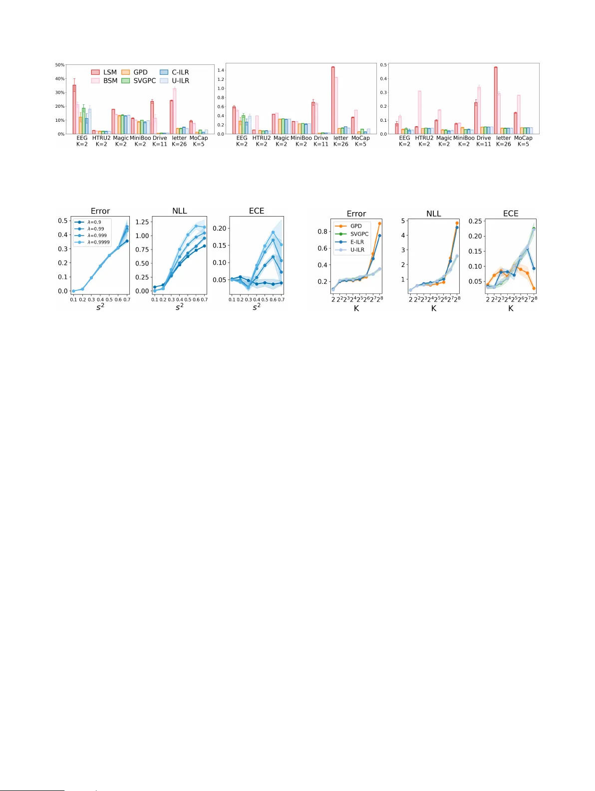
Simplex-to-Euclidean Bijection f or Conjugate and Calibrated Multiclass Gaussian Pr ocess Classification Bernardo W illiams 1 Harsha V ardhan T etali 1 Arto Klami 1 Marcelo Hartmann 1 1 Department of Computer Science, Univ ersity of Helsinki, Finland Abstract W e propose a conjugate and calibrated Gaussian process (GP) model for multi-class classification by exploiting the geometry of the probability sim- plex. Our approach uses Aitchison geometry to map simplex-v alued class probabilities to an un- constrained Euclidean representation, turning clas- sification into a GP regression problem with fewer latent dimensions than standard multi-class GP classifiers. This yields conjugate inference and re- liable predicti ve probabilities without relying on distributional approximations in the model con- struction. The method is compatible with standard sparse GP regression techniques, enabling scal- able inference on larger datasets. Empirical results sho w well-calibrated and competitive performance across synthetic and real-world datasets. 1 INTR ODUCTION Gaussian processes (GPs) [W illiams and Rasmussen, 2006] are attracti ve probabilistic models for supervised learning: they pro vide well-principled uncertainty quantification and often perform strongly in small-data regime. In multi-class classification with K categories, ho we ver , the standard GP approach introduces a v ector of latent functions (typically one per category) and maps them to class probabilities with a link function such as the softmax [Williams and Barber, 1998]. This yields a non-conjugate likelihood, so posterior inference and parameter learning need approximati ve tech- niques such as v ariational inference, Laplace approxima- tion, or Markov chain Monte Carlo [Nickisch et al., 2008, Hensman et al., 2015b, Hernández-Lobato and Hernández- Lobato, 2016]. For man y applications, two desiderata are especially impor- tant: (i) sharp and reliable calibration of predicti ve probabil- ities [Niculescu-Mizil and Caruana, 2005, Guo et al., 2017], and (ii) inference procedures that are exact giv en the model (i.e., conjugate), rather than relying on v ariational approxi- mations in the model construction. From the perspectiv e of inference, notable effort has been made to retain conjugacy in v arious forms. The simplest approaches model discrete la- bels via direct GP re gression [Fröhlich et al., 2013], whereas W enzel et al. [2019] and Galy-F ajou [2022] introduced aux- iliary v ariables to obtain conditional conjugacy and enable Gibbs sampling from conditionally conjugate marginals. Dirichlet-based GP classification (GPD) by Milios et al. [2018] gets closest to offering a fully conjugate solution, av oiding auxiliary variables by using a gamma reparameter - ization for a Dirichlet distribution. Ho wev er , they still need to approximate the gamma distrib utions with log-normal distributions for conjugac y . In practice, many of these methods exhibit poor calibra- tion. Direct GP regression is reported to be very poorly calibrated without additional scaling [Milios et al., 2018], and while robust variants based on Heaviside likelihoods improv e robustness to outliers [Hernández-Lobato et al., 2011, V illacampa-Calvo et al., 2021] they remain poorly calibrated. Overall, v ariational GP classification [Hensman et al., 2015a] and GPD typically pro vide the best calibration in practice. In this work, we present a method that is fully conjug ate without relying on any augmentation or approximations but retains good calibration, revisiting GP classification from the perspecti ve of the geometry of probability vectors. Class probabilities liv e on the simplex, i.e., the set of nonnegati ve vectors in R K whose entries sum to one. This space is natu- rally studied in compositional data analysis [Atchison and Shen, 1980, Aitchison, 1982, Egozcue et al., 2003] which has recently been used in generati ve modeling on the sim- plex [Diederen and Zamboni, 2025, W illiams et al., 2026, Chereddy and Femiani, 2025]. Utilizing Aitchison geome- try , we use the simple x-to-Euclidean bijection of Egozcue et al. [2003] to map probability vectors to an unconstrained Euclidean representation. This allows us to replace discrete labels with continuous Gaussian pseudo-observations in Eu- Data Likelihood Posterior Figure 1: Illustration of Exact-ILR on a K = 3 toy problem. T op (data): Ground-truth class probabilities (blue, green and red), π ( x ) ov er x ∈ [ − 1 , 1] , and three test inputs x (1:3) ∗ . Middle (likelihood): Discrete labels are represented by Gaussian pseudo-observations centered at m ( k ) = φ ( µ ( k ) ) in Euclidean space (Sec. 3), where µ ( k ) = λ e k +(1 − λ ) 1 K 1 . The three panels visualize this class-weighted latent-space likelihood at x (1:3) ∗ . Bottom (posterior): For each x ( i ) ∗ , we draw posterior samples of the latent GP , map them through φ − 1 , and plot the resulting samples of π ∗ . Each point is one sampled probability vector (color = arg max class) and the av erage is ¯ π ( i ) ∗ . The two lo wermost panels show the posterior ov er the two latent GP coordinates across x ∈ [ − 1 , 1] , with training points ov erlaid. clidean space and reduce multi-class classification to GP regression in D := K − 1 latent dimensions. The resulting model is fully conjugate in Euclidean space: posterior inference and learning can be performed exactly using the standard GP marginal likelihood, with the usual exact GP regression cost of O ( N 3 ) ; see Fig 1 for an illus- tration. Concretely , we use the Isometric log-ratio bijection of Egozcue et al. [2003] to define a GP prior ov er a D di- mensional Euclidean latent representation, and we train the model via standard GP re gression machinery on Gaussian pseudo-observations deriv ed from class labels. Compared to Dirichlet-based GP classification [Milios et al., 2018], this yields a conjugate model without introducing a distri- butional approximation in the construction and reduces the number of latent processes from K to D . Because the re- sulting learning problem is GP regression in a transformed space, it can le verage essentially an y sparse GP re gression technique (e.g., inducing-point methods) when scaling be- yond the e xact O ( N 3 ) setting [Titsias, 2009, Hensman et al., 2013]. Our main empirical observ ation is that there are very lar ge differences in ho w well GP classifiers are calibrated, with ours and DGP by Milios et al. [2018] being consistently the best methods with a clear gap between them and the rest. In other words, we pro vide a new model that is fully conjugate and empirically performs extremely well, b ut the empirical improv ement over the strong baseline of DGP is small. 2 B A CKGR OUND Gaussian Process classification W e consider multi-class classification with data D = { ( x n , c n ) } N n =1 , where x n ∈ R P and c n ∈ { 1 , . . . , K } . Let D := K − 1 denote the intrinsic dimension of the simple x. W e denote the (closed) probability simplex ∆ D := { π ∈ R K ≥ 0 : P K k =1 π k = 1 } and its interior ˚ ∆ D := { π ∈ R K > 0 : P K k =1 π k = 1 } . The goal is to estimate the unknown class probabilities π ( x ) = ( π 1 ( x ) , . . . , π K ( x )) ∈ ∆ D , c | x ∼ Cat  π ( x )  . That is, π ( · ) is an unknown function that maps input co vari- ates x to a probability vector for the K categories, and we aim to learn/estimate this mapping from data. A standard GP classifier introduces latent functions and a link function, typically f ( x ) = ( f 1 ( x ) , . . . , f K ( x )) ∈ R K , π ( x ) = softmax  f ( x )  , (1) with independent GP priors on the components, f k ( · ) ∼ G P  0 , K θ ( · , · )  , k ∈ { 1 , . . . , K } , where K θ is a kernel with hyperparameters θ . The posterior is non-conjugate due to the softmax likelihood, so inference is usually approximate, e.g., scalable v ariational inference with inducing points [Hensman et al., 2015a]. Dirichlet-based Gaussian process classification (GPD) Milios et al. [2018] proposed Dirichlet-based Gaussian pro- cess classification (GPD) as a conjugate and calibrated ap- proach to multi-class classification. The model places a Dirichlet distribution on the probability v ector , π ( x ) | x ∼ Dir  α ( x )  , c | x ∼ Cat  π ( x )  . Gi ven an observed class c = k , GPD uses a smoothed target mean and a concentration vector µ ( k ) := ε e k + (1 − ε ) 1 K 1 , α := α 0 µ ( k ) , with α 0 := 1 + K α ε and ε := (1 + K α ε ) − 1 for some α ε > 0 . This yields α k = 1 + α ε and α j = α ε for j  = k . As α ε → 0 , the Dirichlet distribution concentrates on the corresponding one-hot vertex e k : its marginal variances shrink and mass mo ves to the simple x boundary . In practice, the authors suggest α ε is chosen by validation. This method decomposes the Dirichlet distrib ution into in- dependent Gamma distributions g j ind ∼ Gamma( α j , 1) , so that π j = g j / P ℓ g ℓ is distributed Dir( α ) . Matching the first two moments of g j with a log-normal approximation Lognormal( ˜ y j , ˜ σ 2 j ) yields ˜ σ 2 j = log  1 + 1 α j  , ˜ y j = log α j − 1 2 ˜ σ 2 j . (2) Equiv alently , in log-space, log g j ≈ N ( ˜ y j , ˜ σ 2 j ) , so the problem becomes conjugate after the log transform: one fits K independent GPs, each f j to pseudo-observ ations ˜ y nj with a heteroscedastic Gaussian likelihood whose noise variances ˜ σ 2 nj depend on the (label-dependent) Dirichlet parameters α nj for n = 1 , .., N . This view is close in spirit to our approach by also leveraging Gaussian regression in a transformed space. At a test input x ∗ , letting f ∗ ∈ R K denote the latent GP , GPD approximates predictiv e probabilities by Monte Carlo, E [ π ∗ | x ∗ , D ] ≈ 1 S S X s =1 softmax  f ( s ) ∗  , f ( s ) ∗ ∼ p ( f ∗ | x ∗ , D ) . 3 METHOD W e propose a conjugate and calibrated GP classification model by mapping probability vectors on the simplex to Eu- clidean space, and con verting classification into regression by assigning each class a latent tar get location and learn- ing a GP that interpolates these tar gets. The construction follows the same high-lev el idea as GPD, b ut it av oids the log-normal approximation and uses D := K − 1 latent dimensions, one less than GPD. GPD models π | x ∼ Dir( α ( x )) with a GP . W e instead, model class probabilities through a latent Euclidean rep- resentation of the open simplex. W e choose a bijection φ : ˚ ∆ D → R D and learn a latent GP for f ( x ) ∈ R D , and ev entually the class probabilities are estimated by mapping back to the simplex with ˜ π ( x ) := φ − 1  f ( x )  ∈ ˚ ∆ D . T o train the model, each discrete label c = k is associated with a class target m ( k ) ∈ R D obtained by mapping a smoothed one-hot vector µ ( k ) through φ . W e then fit f by GP regression to these latent targets under a Gaussian likelihood with a fixed variance σ 2 . This yields conjugate inference. The precise choices of φ , µ ( k ) , m ( k ) , and σ 2 are giv en next. Figure 2: Likelihood in simplex and Euclidean spaces. The likelihood of observing classes 1 , 2 , or 3 at input x is a Gaussian mixture with modes at m ( k ) = φ ( µ ( k ) ) in Eu- clidean space (right), which induces a pushforward likeli- hood on the simplex (left). The figure sho ws the likelihood for π ( x ) = (1 / 3 , 1 / 3 , 1 / 3) . 3.1 ILR-GA USSIAN PROCESS W e now make the construction concrete. W e (i) choose φ to be the isometric logratio (ILR) bijection and (ii) specify how each class label is embedded as a latent target with an adequate amount Gaussian noise. W e build on the idea recently proposed by W illiams et al. [2026] where a similar interpolation and simplex-to-Euclidean bijections was used for generativ e modeling of discrete data using flows. Giv en a label c = k , we map the one-hot vector to the simplex interior with the interpolation µ ( k ) := λ e k + (1 − λ ) 1 K 1 ∈ ˚ ∆ D , λ ∈ (0 , 1) , define the corresponding latent tar get m ( k ) := φ  µ ( k )  , and use the latent-space likelihood z | ( c = k , x ) ∼ N  m ( k ) , σ 2 I D  , (3) where σ 2 is fixed (and chosen by a principled rule; see Proposition 1). Mapping back through φ − 1 induces the simplex-v alued pushforward likelihood (see Fig. 2 for an illustration), π | ( c = k , x ) ∼ ( φ − 1 ) # N  m ( k ) , σ 2 I D  . T raining reduces to GP re gression with a GP prior in R D and the likelihood giv en in Equation 3. The posterior is Gaussian, inference is conjugate on R D and class probabilities are generated by mapping to ˚ ∆ D with φ − 1 (full details provided in Sec. 3.2). The main design choices are the mapping φ and the noise le vel σ 2 , which controls the class ov erlap in the latent space. In our experiments, we select λ by validation. ILR map and Aitchison geometry Here, we briefly in- troduce Aitchison geometry and the associated ILR bijec- tion, which maps the open simplex to Euclidean space. This framew ork provides a principled notion of norms and dis- tances between probability vectors on the simple x, and the ILR map giv es Euclidean coordinates that preserv e these distances. W e will later use this geometry to define a suitable noise le vel in the likelihood (Proposition 1) by quantifying the separation between the latent class tar gets m ( k ) in a con- sistent way . W e equip the open simplex with the Aitchison inner product [Aitchison, 1982]. For x , y ∈ ˚ ∆ D , ⟨ x , y ⟩ A := 1 2 K K X i,j =1 log x i x j log y i y j . This inner product induces the norm ∥ x ∥ A := p ⟨ x , x ⟩ A and the Aitchison distance d A ( x , y ) := v u u t 1 2 K K X i,j =1  log x i x j − log y i y j  2 . The isometric logratio (ILR) transform [Egozcue et al., 2003] provides e xplicit Euclidean coordinates that respect this geometry . Let H ∈ R D × K be the Helmert matrix [Lan- caster, 1965] and define φ : ˚ ∆ D → R D , y 7→ z = H log y , φ − 1 : R D → ˚ ∆ D , z 7→ y = softmax  H ⊤ z  , (4) where log is applied elementwise. The ILR mapping is an isometry between ( ˚ ∆ D , d A ) and ( R D , ∥ · ∥ 2 ) , so Euclidean distances in latent space correspond e xactly to Aitchison distances on the simplex. This makes it con venient to place a Gaussian likelihood and a GP prior on z ∈ R D while pre- serving the simplex-geometry notion of separation between probability vectors. The complexity of the ILR-transform is linear on the number of classes O ( K ) , due to the special form of the Helmert matrix. Other dif feomorphic log-ratio maps such as the additi ve log-ratio or multiplicativ e log- ratio can also be used [Aitchison, 1981, 1982], but these mappings depend on the order of the input, giving a different map for different permutations and are not isomorphic. How to choose σ 2 ? The v ariance σ 2 controls ho w much ov erlap there is between pseudo-observations of different classes in latent space. W e find an upper bound for the vari- ance that limits the ov erlap to a gi ven tolerance probability ϵ . W e can select any value of σ between zero and the upper bound, but in practice choose σ as the upper bound value, and a smaller v alue can be chosen by reducing the ov erlap tolerance. Marginalizing the (unknown) class label, our pseudo- observation model corresponds to a Gaussian mixture, p ( z | x ) = K X k =1 p ( z , c = k | x ) = K X k =1 p ( c = k | x ) p ( z | c = k , x ) = K X k =1 π k ( x ) N  z | φ ( µ ( k ) ) , σ 2 I D  . T o control component overlap, we use the f act that the ILR map φ is an isometry: Euclidean distances between compo- nent means in latent space equal Aitchison distances on the simplex. W e define the (common) pairwise separation δ := d A  µ ( k ) , µ ( ℓ )  = ∥ m ( k ) − m ( ℓ ) ∥ 2 , k  = ℓ, and deri ve Proposition 1 as a suf ficient condition for negli- gible intersection between mixture components. Proposition 1 (Choice of σ for negligible component in- tersection) . Let K ≥ 2 . Define, for each class k ∈ { 1 , . . . , K } , m ( k ) := φ  µ ( k )  ∈ R D . Let δ := min k  = ℓ ∥ m ( k ) − m ( ℓ ) ∥ , which equals the corr esponding Aitchison distance between the class center s on the simplex by the ILR isometry . Let V k := { z ∈ R D : ∥ z − m ( k ) ∥ ≤ ∥ z − m ( ℓ ) ∥ ∀ ℓ } . F or any ε ∈ (0 , 1) , if σ ≤ δ 2 z 1 − ε/D , z q := Φ − 1 ( q ) , (5) then for every x and every k , P  Z / ∈ V k   C = k , x  ≤ ε , wher e C denotes the class label and Z ∼ N ( m ( k ) , σ 2 I D ) . 3.2 TRAINING AND PREDICTION Exact Gaussian process model (Exact-ILR) W e place a GP prior on a latent function f ( · ) ∈ R D and use a Gaussian likelihood, f ( · ) ∼ G P ( 0 , K θ ) , z i | f ( x i ) ∼ N  f ( x i ) , σ 2 I D  . This is standard multi-output GP regression (with indepen- dent outputs), hence the posterior inference and predictions are closed-form. This is the exact (non-sparse) v ariant used in our experiments. W e follo w Milios et al. [2018] and share the kernel’ s parameters across all dimensions. W e infer the kernel hyperparameters θ by maximizing the (Gaussian) marginal likelihood p ( { z i } N i =1 | { x i } N i =1 , θ ) . Concretely , letting X := ( x 1 , . . . , x N ) and K N := K θ ( X , X ) ∈ R N × N , the model factorizes over ILR coordinates d ∈ { 1 , . . . , D } . Writing z ( d ) := ( z 1 d , . . . , z N d ) ⊤ and defin- ing the shorthand ∥ v ∥ 2 A := v ⊤ A − 1 v , the marginal log- likelihood decomposes as log p  z | θ  = − 1 2 D X d =1 ∥ z ( d ) ∥ 2 ( K N + σ 2 I N ) − 1 − D 2 log | K N + σ 2 I N | , where we omit the additi ve constant − N D 2 log(2 π ) since it does not af fect optimization. For a test input x ∗ , with k ∗ := K θ ( X , x ∗ ) and k ∗∗ := K θ ( x ∗ , x ∗ ) , the predictive latent is f ( d ) ∗ | z ( d ) , X ∼ N  µ ( d ) ∗ , σ 2 ∗  , µ ( d ) ∗ := k ⊤ ∗ ( K N + σ 2 I N ) − 1 z ( d ) , σ 2 ∗ := k ∗∗ − k ⊤ ∗ ( K N + σ 2 I N ) − 1 k ∗ . Collecting coordinates, f ∗ | D ∼ N ( µ ∗ , Σ ∗ ) with µ ∗ := ( µ (1) ∗ , . . . , µ ( D ) ∗ ) ⊤ and Σ ∗ := σ 2 ∗ I D . Predictions in probability space Gi ven the Gaussian pre- dictiv e latent distribution f ∗ | D ∼ N ( µ ∗ , Σ ∗ ) from the previous paragraph, we map samples back to the simplex and estimate the predicti ve probabilities as an expectation with Monte Carlo, E [ π ∗ | x ∗ , D ] ≈ 1 S S X s =1 φ − 1  f ( s ) ∗  f ( s ) ∗ ∼ N ( µ ∗ , Σ ∗ ) . (6) W e then predict the class via ˆ c = arg max k E [ π ∗ ,k | x ∗ , D ] . 3.3 SP ARSE GA USSIAN PROCESSES Exact GP inference scales cubically in N and is prohibitiv e for large datasets. W e therefore use inducing-point approxi- mations; in what follows we outline the tw o sparse alterna- tiv es used in our experiments: an uncollapsed sparse v aria- tional classifier (Uncollapsed-ILR) and a collapsed sparse GP model (Collapsed-ILR). Let X u := { x u m } M m =1 be in- ducing inputs and, for each latent GP output f ( d ) , define inducing variables u ( d ) := f ( d ) ( X u ) . The inducing loca- tions X u are treated as parameters and optimized jointly with kernel hyperparameters. Sparse variational GP Classification (Uncollapsed-ILR) W e consider the sparse variational GP classifier of Hens- man et al. [2015a], which is often informally referred to as “uncollapsed” because its lower bound is additive ov er data points, enabling stochastic optimization. Instead of using the softmax as the link function we propose using the bijection φ . This choice again reduces to only D la- tent GPs, compared to the standard softmax parameteri- zation (see Eq. 1). The class probabilities are parameter- ized as π ( x ) = φ − 1 ( f ( x )) for f ( x ) ∈ R D . Using induc- ing v ariables u := ( u (1) , . . . , u ( D ) ) , we use a mean-field Gaussian variational posterior q ( u ) = Q D d =1 q ( u ( d ) ) with q ( u ( d ) ) = N ( u ( d ) | m ( d ) , S ( d ) ) . W e follow Hensman et al. [2015a] to define q ( f ) := R p ( f | u ) q ( u ) d u , which im- plies Gaussian marginals q ( f i ) at the training inputs. Param- eters { m ( d ) , S ( d ) } , X u , θ , are learned by maximizing the stochastic variational objecti ve log p ( c ) ≥ N X i =1 E q ( f i )  log p ( c i | f i )  − D X d =1 KL  q ( u ( d ) ) ∥ p ( u ( d ) )  . W e optimize this objecti ve using mini-batches; the e x- pectation under the categorical likelihood p ( c i | f i ) = Cat( φ − 1 ( f i )) is approximated numerically by Monte Carlo. At prediction time, q ( f ∗ ) is obtained from the variational posterior (a Gaussian with closed-form mean/cov ariance), and probabilities follo w from Monte Carlo through φ − 1 . W e refer to this model as Uncollapsed-ILR. In our experiments, we also include an additional learnable weight matrix W [Alvarez et al., 2012]. F or softmax-based classifiers we use π ( x ) = softmax( Wf ( x )) , and in our case we use π ( x ) = φ − 1 ( Wf ( x )) . This parameter is opti- mized jointly with the others w .r .t. the lower bound. Sparse GP (Collapsed-ILR) F or our ILR model, the bi- jection and our modeling choice give a latent Gaussian like- lihood in R D : p ( z | f ( x )) = N ( z | f ( x ) , σ 2 I D ) . W e can therefore follo w Milios et al. [2018] and use the approach of T itsias [2009] to construct a "collapsed" variational ap- proximation. It uses D latent GPs (one per ILR coordinate) and inducing v ariables u . The inducing points together with the model parameters are optimized with the lower bound: log p ( z ) ≥ log N  z | 0 , Q N + σ 2 I N  − 1 2 σ 2 tr( K N − Q N ) , where Q N = K N M K − 1 M K M N . This reduces the cost to O ( N M 2 ) , we note that we could also hav e reduced the cost by introducing minibatches with an additional Gaussian ap- proximation as in Hensman et al. [2013] but decided to use the method of Titsias [2009] to keep the results comparable to Milios et al. [2018]. 4 RELA TED WORK The standard multi-class GP classifier combines K latent GPs with a softmax link [W illiams and Barber, 1998], which yields a non-conjugate likelihood and motiv ates approx- imate inference. Classic approximations include Laplace and related methods [Nickisch et al., 2008], as well as ex- pectation propagation [Hernández-Lobato and Hernández- Lobato, 2016, V illacampa-Calvo and Hernández-Lobato, 2017] and variational inference with inducing points [Hens- man et al., 2015a,b]. Recent work has continued to e xpand the modeling and scalability of multi-class GP classifica- tion, for example by handling various likelihoods [Liu et al., Figure 3: Error , NLL and ECE for UCI datasets in the exact setting. 2019], incorporating input noise [V illacampa-Calvo et al., 2021], or using transformed constructions for non-stationary and dependent outputs [Maroñas and Hernández-Lobato, 2023]. There is also an acti ve line of work on deep GP mod- els for classification [Blomqvist et al., 2019, Dutordoir et al., 2020] and on robustness considerations [Hernández-Lobato et al., 2011, Blaas et al., 2020]. There are GP classifica- tion models that achieve conditional conjugacy by data- augmentation [W enzel et al., 2019, Galy-Fajou et al., 2020]. Galy-Fajou [2022, Chapter 7] realized that the method of Galy-Fajou et al. [2020] can use D latent GPs instead of K . They consider a different link function from ours, we use the ILR bijection and bypass the need for auxiliary variables and Gibbs sampling, making the classification problem a regression problem in the latent space. 5 EXPERIMENTS W e ev aluate our approach on synthetic and real-world benchmarks to assess predictive accuracy and calibration. W e compare against Dirichlet-based Gaussian processes (GPD) [Milios et al., 2018], Logistic Softmax (LSM) [Galy- Fajou et al., 2020], Bijecti ve Softmax (BSM) [Galy-F ajou, 2022], and sparse variational Gaussian process classifica- tion (SVGPC) [Hensman et al., 2015a]. Throughout the experiments, “e xact” denotes the non-sparse setting, where posterior inference is done directly for the corresponding latent/augmented model: for our method and GPD via direct Gaussian latent posterior computations, and for LSM/BSM via Gibbs sampling in the augmented model. “sparse” de- notes inducing-point approximations. F or GPD, LSM and BSM we consider both exact and sparse settings. For our method, we ev aluate one exact variant (Exact-ILR) and two sparse v ariants (Collapsed-ILR and Uncollapsed-ILR). In the plots, for space reasons, we use the short labels E- ILR, C-ILR, and U-ILR for Exact-ILR, Collapsed-ILRand Uncollapsed-ILR. The implementation code is av ailable in the supplementary material. W e use independent zero-mean GP priors with an RBF ker- nel K θ for all methods, K θ ( x, x ′ ) = σ 2 f exp  − ∥ x − x ′ ∥ 2 2 2 ℓ 2  , with hyperparameters θ = ( σ 2 f , ℓ ) . W e report accuracy , negati ve log-likelihood (NLL), and e x- pected calibration error (ECE) on a test set. The NLL is the categorical cross entrop y NLL := − 1 n P n i =1 log ˆ π i,c i . ECE [Guo et al., 2017] is computed with M = 10 equally spaced bins over a confidence score. For binary classification we compute the confidence for class c = 1 , and for multi-class classification ( K > 2 ) we use the standard top-label confi- dence ˆ p i := max k ˆ π i,k , yielding ECE := M X m =1 | B m | n   acc( B m ) − conf ( B m )   , where conf ( B m ) := 1 | B m | P i ∈ B m ˆ p i . W e fix the toler- ance parameter ε = 10 − 6 (as in Proposition 1) for all experiments. Unless stated otherwise, we report results as the mean and one standard deviation over 5 random train/validation/test splits (seeds). UCI classification in the exact setting W e ev aluate meth- ods in the exact setting on three small UCI datasets from Hernández-Lobato et al. [2011], each with fe wer than 300 samples, where exact O ( N 3 ) inference is feasible. For each seed, we set aside 50 points as a test set and use 10% of the remaining training data as a validation set. W e tune the label- smoothing parameter ov er λ ∈ { 0 . 95 , 0 . 99 , 0 . 999 , 0 . 9999 } and select the best v alue based on validation NLL. For GPD, we tune α ε ∈ { 0 . 1 , 0 . 01 , 0 . 001 , 0 . 0001 } and again select the model’ s parameters by validation NLL. Figure 3 shows that our method and GPD achie ve similar ac- curacy , while our method attains slightly lower NLL on two of the three datasets and the lowest ECE on all three, mean- ing it is slightly better calibrated. LSM and BLM perform worse than the non-augmented models. UCI classification benchmarks in the sparse setting W e replicate the UCI benchmarks from Milios et al. [2018] on 7 classification tasks, which require sparse inference due to dataset sizes ranging from tens of thousands to hundreds of thousands of points. W e use a validation set consisting of 10% of the training data to select hyperparameters. W e tune λ ∈ { 0 . 95 , 0 . 99 , 0 . 999 , 0 . 9999 , 0 . 999999 } and choose the value that minimizes v alidation NLL; for GPD we tune α ε ∈ { 0 . 1 , 0 . 01 , 0 . 001 , 0 . 0001 } and again select by vali- dation NLL. For optimization, we try learning rates 10 − 2 and 10 − 3 for all methods, and we report the best setting on the validation set. W e additionally consider two standard input preprocessing variants ( − 1 to 1 ) and unit-variance normalization) for all methods. W e initialize inducing points with k -means++ [Arthur and V assilvitskii, 2006]; the number of inducing points and dataset-specific details follow Milios et al. [2018] and are reported in the appendix. F or SV GPC and Uncollapsed-ILR, we include an additional learnable mixing matrix W before the link function (Sec. 3.3). For sparse "collapsed" GPD and sparse Collapsed-ILR, we also consider a more flexible (a) Error rate (b) Negati ve log-likelihood (c) Expected Calibration Error Figure 4: Sparse models performance on datasets from the UCI repository . Figure 5: Error , NLL and ECE for increasing overlap of the input variables. likelihood by adding an extra per -class scale parameter to the observation noise. Figure 4 summarizes the results (see App. B for the detailed numerical values). Ov erall, sparse GPD and Collapsed-ILR achiev e strong performance across metrics. The ILR-based sparse v ariants (Collapsed-ILR and Uncollapsed-ILR) are better in terms of ECE on 3 out of the 7 tasks and are other- wise comparable to their softmax/Dirichlet counterparts. On the L E T T E R dataset Uncollapsed-ILR is better than Exact- ILR. The data-augmented methods LSM and BSM struggle across all metrics, especially for more than 2 categories. In summary , our sparse methods are similar in performance to sparse GPD, while sometimes being slightly better cali- brated. Effect of the parameter λ W e replicate the setup of Galy- Fajou et al. [2020] to ev aluate how the label-smoothing parameter λ affects calibration as the class assignment becomes less clear . W e consider a synthetic dataset with K = 3 classes where the covariates are generated from a mixture model (one component per class) and control class ambiguity by varying the component standard deviation s ∈ { 0 . 1 , . . . , 0 . 7 } . As s 2 increases, the components over - lap and the conditional class probabilities become close to uniform ov er large parts of the covariate space (e.g., for s = 0 . 7 almost all inputs are plausibly generated by multi- ple components). In this regime, a well-calibrated classifier should output near-uniform predicti ve probabilities except in small regions where one component clearly dominates Figure 6: Error , NLL and ECE for increasing number of categories K . and the model should be confident. Fig. 5 sho ws that NLL and ECE v ary with λ , especially at higher ov erlap. Across noise levels s 2 , we find that λ = 0 . 9 yields the most stable calibration and best error and NLL, whereas larger values tend to become overconfident when the inputs are ambiguous. For lo wer noise lev els (small s 2 ), higher values of λ perform better , as the model can be more confident. Since the optimal λ is problem-dependent, in the remaining experiments we select λ using a validation set. Scaling with the number of categories W e next study how performance changes as the number of classes gro ws. For K ∈ { 2 , 4 , . . . , 256 } , we generate a 2 -dimensional in- put classification problem where each class corresponds to one component in a Gaussian mixture with means placed ev enly around the unit circle. W e choose a shared v ariance so that nearby components have non-tri vial overlap; this en- sures that the Bayes-optimal classifier is not always certain and that a well-calibrated model should express uncertainty in regions where multiple classes are plausible. For each v alue of K , we use N = 1000 training points and 1000 test points. W e tune the label-smoothing pa- rameter over λ ∈ { 0 . 95 , 0 . 99 , 0 . 999 , 0 . 9999 } and report the v alue that minimizes training NLL. F or GPD, we similarly tune the concentration parameter ov er α ε ∈ { 0 . 1 , 0 . 01 , 0 . 001 , 0 . 0001 } using training NLL. For the sparse v ariational baselines (SV GPC and Uncollapsed-ILR), we use M = 128 inducing points selected with k -means++. Figure 6 summarizes the results. SVGPC and Uncollapsed- ILR exhibit v ery similar performance across K , indicating that the ILR parameterization works as well as the sparse variational baseline, and the they are the most accurate for K > 2 6 . Exact-ILR is as accurate as GPD for K ≤ 2 6 and slightly more accurate for K > 2 6 . It is better calibrated than GPD for K = 2 2 to 2 5 but less calibrated for K > 2 6 . When does GPD break do wn? This experiment high- lights an often-overlook ed choice in Dirichlet-based GP classification (GPD): whether to form predicti ve probabil- ities from the latent GP predictiv e p ( f ∗ | D , x ∗ ) or from the predicti ve distrib ution of the noisy pseudo-observ ation p ( z ∗ | D , x ∗ ) (i.e., including the likelihood noise). Con- cretely , in GPD one can estimate probabilities either as π ∗ ≈ softmax( f ∗ ) with f ∗ ∼ p ( f ∗ | D , x ∗ ) , or as π ∗ ≈ softmax( z ∗ ) with z ∗ ∼ p ( z ∗ | D , x ∗ ) . For our method, the analogous choice is whether to apply φ − 1 to samples from p ( f ∗ | D , x ∗ ) or from p ( z ∗ | D , x ∗ ) . W e consider the same synthetic setup as the Galy-Fajou et al. [2020] and focus on an easy regime where both models fit perfectly when using the latent predictive: we fix λ = 0 . 9 , set α ε = 0 . 01 , and choose s = 0 . 1 so the mixture components are well separated. T able 1 reports test error when we estimate π ∗ using a single Monte Carlo sample (Eq. 6) under the two choices. While both methods achiev e zero error when predicting via p ( f ∗ | D , x ∗ ) , using p ( z ∗ | D , x ∗ ) can introduce av oidable misclassifications for GPD. This behavior is a consequence of estimating the probabili- ties from noisy pseudo-observ ations under the log-normal approximation: sampling z ∗ adds variability before the soft- max, and fluctuations can move a sample into a different arg max region. The size of this ef fect depends on both K and α ε . As K increases, there are more competing classes, so the probability that some incorrect coordinate becomes the maximum increases. Meanwhile, our numerical esti- mates (see Appendix B) sho w that the error from using p ( z ∗ | D , x ∗ ) decreases as α ε becomes smaller . In prac- tice, averaging o ver multiple samples reduces the effect, and using the latent predictiv e p ( f ∗ | D , x ∗ ) works well for both methods. For Exact-ILR, we additionally choose σ 2 to make the probability of crossing decision boundaries in latent space negligible (Proposition 1), which e xplains the robustness observ ed here. 6 CONCLUSION W e introduced a new conjugate multiclass Gaussian pro- cess classification model that represents class probabilities on the simplex and uses the ILR bijection to work in a D = K − 1 dimensional Euclidean latent space. This turns classification into standard multi-output GP re gres- sion with a Gaussian likelihood on latent targets, yield- ing closed-form posterior inference and exact marginal- Model Error ( y ∗ ) Error ( f ∗ ) GPD 0 . 076 ± 0 . 013 0 . 0 ± 0 . 0 Exact-ILR 0 . 0 ± 0 . 0 0 . 0 ± 0 . 0 T able 1: T est misclassification rate when forming π ∗ from either the noisy predictiv e distribution p ( z ∗ | D , x ∗ ) or the latent predicti ve p ( f ∗ | D , x ∗ ) . For GPD we compute π ∗ = softmax( · ) , applying softmax to samples of either z ∗ or f ∗ . For Exact-ILR we compute π ∗ = φ − 1 ( · ) , applying φ − 1 to samples of either z ∗ or f ∗ . likelihood learning with O ( N 3 ) complexity in the number of training points. Importantly , our results highlight a clear empirical gap between simple x-based models (Exact-ILR, Collapsed-ILR, and GPD) and auxiliary-variable and sparse variational GP classifiers in both the exact and sparse set- tings. Across experiments, the simple x-based models consis- tently achie ve stronger accuracy , calibration, and robustness, while auxiliary-v ariable methods generally lag behind and sparse v ariational approaches can underperform in some scenarios. This motiv ates the use of our method on tasks where reliable uncertainty calibrated estimates are crucial. W ithin the class of well-calibrated, conjugate models, our method offers a principled alternativ e to Dirichlet-based GP classification, achie ving conjugacy without relying on the log-normal approximation to the Gamma construction, while delivering comparable or slightly improv ed calibra- tion without sacrificing accuracy . Discussion and outlook. From a methodological stand- point, reducing multiclass classification to GP regression in latent ILR coordinates pro vides a simple and scalable framew ork. Because the core problem becomes standard multi-output GP regression, existing advances in scalable GP inference can be used directly . In this w ork we employed inducing-point v ariational methods [T itsias, 2009, Hensman et al., 2015a], b ut the same formulation is compatible with more recent sparse and variational constructions [Salimbeni et al., 2018, Hensman et al., 2018, Shi et al., 2020, Rossi et al., 2021, W enger et al., 2022b], iterative linear -algebra solvers for approximate GP inference [W ang et al., 2019, W ilson et al., 2021, W enger et al., 2022a, Lin et al., 2024], and structured kernel interpolation and related kernel rep- resentations [W ilson and Nickisch, 2015, Gardner et al., 2018b]. Our formulation introduces only a small number of interpretable design choices, notably the label-smoothing parameter λ and the latent noise lev el σ 2 , which we se- lected using validation or principled o verlap bounds; future work could consider adaptiv e (e.g., input or class depen- dent) choices while retaining tractable inference. Overall, the proposed construction provides a modular way to com- bine well-calibrated multiclass GP classification with GP regression tools, including scalable solvers, structured k er- nels, and richer priors, in larger and more complex settings. Acknowledgements The authors were supported by the Research Council of Finland Flagship programme: Finnish Center for Artificial Intelligence FCAI, and additionally by grants: 363317 (BW , AK), 369502 (MH). The authors acknowledge the research en vironment provided by ELLIS Institute Finland, and CSC - IT Center for Science, Finland for computational resources. References John Aitchison. A new approach to null correlations of proportions. Journal of the International Association for Mathematical Geology , 13(2):175–189, 1981. John Aitchison. The statistical analysis of compositional data. Journal of the Royal Statistical Society: Series B (Methodological) , 44(2):139–160, 1982. Mauricio A Alv arez, Lorenzo Rosasco, and Neil D Lawrence. Kernels for vector -valued functions: A re- view . F oundations and T rends® in Mac hine Learning , 4 (3):195–266, 2012. David Arthur and Sergei V assilvitskii. k-means++: The adv antages of careful seeding. T echnical report, Stanford, 2006. John Atchison and Sheng M Shen. Logistic-normal distri- butions: Some properties and uses. Biometrika , 67(2): 261–272, 1980. Arno Blaas, Andrea P atane, Luca Laurenti, Luca Cardelli, Marta Kwiatkowska, and Stephen Roberts. Adversar- ial robustness guarantees for classification with gaussian processes. In International Conference on Artificial Intel- ligence and Statistics , pages 3372–3382. PMLR, 2020. Kenneth Blomqvist, Samuel Kaski, and Markus Heinonen. Deep conv olutional gaussian processes. In Joint eur opean confer ence on machine learning and knowledge discovery in databases , pages 582–597. Springer , 2019. Sathvik Reddy Chereddy and John Femiani. Sketchdnn: Joint continuous-discrete diffusion for cad sketch genera- tion. In International Conference on Mac hine Learning , pages 10199–10215. PMLR, 2025. T omek Diederen and Nicola Zamboni. Flows on conv ex polytopes. arXiv preprint , 2025. Dheeru Dua and Casey Graff. Uci machine learning repository , 2017. URL http://archive.ics.uci. edu/ml . V incent Dutordoir , Mark W ilk, Artem Artemev , and James Hensman. Bayesian image classification with deep conv o- lutional gaussian processes. In International Conference on Artificial Intelligence and Statistics , pages 1529–1539. PMLR, 2020. Juan José Egozcue, V era Pawlo wsky-Glahn, Glòria Mateu- Figueras, and Carles Barcelo-V idal. Isometric logratio transformations for compositional data analysis. Mathe- matical geology , 35(3):279–300, 2003. Björn Fröhlich, Erik Rodner , Michael Kemmler , and Joachim Denzler . Large-scale gaussian process multi- class classification for semantic segmentation and facade recognition. Machine vision and applications , 24(5): 1043–1053, 2013. Théo Galy-Fajou. Latent V ariable Augmentation for Appr ox- imate Bayesian Infer ence Applications for Gaussian Pr o- cesses . Phd dissertation, T echnische Universität Berlin, Fakultät IV – Elektrotechnik und Informatik, Berlin, Ger- many , 2022. Théo Galy-Fajou, Florian W enzel, Christian Donner , and Manfred Opper . Multi-class gaussian process classifica- tion made conjugate: Ef ficient inference via data augmen- tation. In Uncertainty in Artificial Intellig ence , pages 755–765. PMLR, 2020. Jacob Gardner, Geoff Pleiss, Kilian Q W einberger , David Bindel, and Andrew G Wilson. Gpytorch: Blackbox matrix-matrix gaussian process inference with gpu ac- celeration. Advances in neural information pr ocessing systems , 31, 2018a. Jacob Gardner , Geof f Pleiss, Ruihan W u, Kilian W einberger , and Andrew W ilson. Product kernel interpolation for scalable gaussian processes. In International Confer ence on Artificial Intelligence and Statistics , pages 1407–1416. PMLR, 2018b. Chuan Guo, Geoff Pleiss, Y u Sun, and Kilian Q W einberger . On calibration of modern neural networks. In Interna- tional confer ence on mac hine learning , pages 1321–1330. PMLR, 2017. James Hensman, Nicolò Fusi, and Neil D. Lawrence. Gaus- sian processes for big data. In Pr oceedings of the T wenty- Ninth Confer ence on Uncertainty in Artificial Intelligence , U AI’13, page 282–290, Arlington, V irginia, USA, 2013. A U AI Press. James Hensman, Alexander Matthe ws, and Zoubin Ghahra- mani. Scalable v ariational gaussian process classification. In Artificial intelligence and statistics , pages 351–360. PMLR, 2015a. James Hensman, Alexander G Matthews, Maurizio Filip- pone, and Zoubin Ghahramani. Mcmc for variationally sparse gaussian processes. Advances in neural informa- tion pr ocessing systems , 28, 2015b. James Hensman, Nicolas Durrande, and Arno Solin. V aria- tional fourier features for gaussian processes. Journal of Machine Learning Resear ch , 18(151):1–52, 2018. Daniel Hernández-Lobato and José Miguel Hernández- Lobato. Scalable gaussian process classification via ex- pectation propagation. In Artificial Intelligence and Statis- tics , pages 168–176. PMLR, 2016. Daniel Hernández-Lobato, Jose Hernández-Lobato, and Pierre Dupont. Robust multi-class gaussian process clas- sification. Advances in neur al information processing systems , 24, 2011. HO Lancaster . The helmert matrices. The American Mathe- matical Monthly , 72(1):4–12, 1965. Jihao Andreas Lin, Shre yas Padhy , Javier Antoran, Austin T ripp, Alexander T erenin, Csaba Szepesvari, José Miguel Hernández-Lobato, and David Janz. Stochastic gradient descent for gaussian processes done right. In The T welfth International Confer ence on Learning Repr esentations , 2024. Haitao Liu, Y e w-Soon Ong, Ziwei Y u, Jianfei Cai, and Xi- aobo Shen. Scalable gaussian process classification with additiv e noise for various likelihoods. arXiv pr eprint arXiv:1909.06541 , 2019. Juan Maroñas and Daniel Hernández-Lobato. Efficient trans- formed gaussian processes for non-stationary dependent multi-class classification. In International Confer ence on Machine Learning , pages 24045–24081. PMLR, 2023. Dimitrios Milios, Raffaello Camoriano, Pietro Michiardi, Lorenzo Rosasco, and Maurizio Filippone. Dirichlet- based gaussian processes for lar ge-scale calibrated clas- sification. Advances in Neural Information Pr ocessing Systems , 31, 2018. Hannes Nickisch, Carl Edward Rasmussen, et al. Approxi- mations for binary gaussian process classification. Jour - nal of Machine Learning Resear ch , 9(10):2035–2078, 2008. Alexandru Niculescu-Mizil and Rich Caruana. Predicting good probabilities with supervised learning. In Pr oceed- ings of the 22nd international confer ence on Machine learning , pages 625–632, 2005. Simone Rossi, Markus Heinonen, Edwin Bonilla, Zheyang Shen, and Maurizio Filippone. Sparse gaussian processes revisited: Bayesian approaches to inducing-v ariable ap- proximations. In International Confer ence on Artificial Intelligence and Statistics , pages 1837–1845. PMLR, 2021. Hugh Salimbeni, Ching-An Cheng, Byron Boots, and Marc Deisenroth. Orthogonally decoupled variational gaussian processes. Advances in neur al information pr ocessing systems , 31, 2018. Jiaxin Shi, Michalis Titsias, and Andriy Mnih. Sparse or- thogonal variational inference for g aussian processes. In International Confer ence on Artificial Intelligence and Statistics , pages 1932–1942. PMLR, 2020. Michalis T itsias. V ariational learning of inducing variables in sparse gaussian processes. In Artificial intellig ence and statistics , pages 567–574. PMLR, 2009. Carlos V illacampa-Calvo and Daniel Hernández-Lobato. Scalable multi-class gaussian process classification using expectation propagation. In International Confer ence on Machine Learning , pages 3550–3559. PMLR, 2017. Carlos V illacampa-Calvo, Bryan Zaldívar , Eduardo C Garrido-Merchán, and Daniel Hernández-Lobato. Multi- class gaussian process classification with noisy inputs. Journal of Machine Learning Researc h , 22(36):1–52, 2021. Ke W ang, Geoff Pleiss, Jacob Gardner , Stephen T yree, Kil- ian Q W einberger , and Andrew Gordon Wilson. Exact gaussian processes on a million data points. Advances in neural information pr ocessing systems , 32, 2019. Jonathan W enger , Geoff Pleiss , Philipp Hennig, John Cun- ningham, and Jacob Gardner . Preconditioning for scal- able gaussian process hyperparameter optimization. In International Conference on Mac hine Learning , pages 23751–23780. PMLR, 2022a. Jonathan W enger , Geoff Pleiss, Marvin Pförtner , Philipp Hennig, and John P Cunningham. Posterior and com- putational uncertainty in gaussian processes. Advances in Neural Information Pr ocessing Systems , 35:10876– 10890, 2022b. Florian W enzel, Théo Galy-Fajou, Christan Donner , Marius Kloft, and Manfred Opper . Efficient gaussian process classification using pòlya-gamma data augmentation. In Pr oceedings of the AAAI Conference on Artificial Intelli- gence , v olume 33, pages 5417–5424, 2019. Bernardo W illiams, V ictor M Y eom-Song, Marcelo Hart- mann, and Arto Klami. Simplex-to-euclidean bijections for categorical flow matching. In International Confer- ence on Artificial Intelligence and Statistics , 2026. Ac- cepted / to appear . Christopher KI W illiams and David Barber . Bayesian clas- sification with gaussian processes. IEEE T ransactions on pattern analysis and machine intellig ence , 20(12):1342– 1351, 1998. Christopher KI W illiams and Carl Edward Rasmussen. Gaussian pr ocesses for machine learning , v olume 2. MIT press Cambridge, MA, 2006. Andrew Wilson and Hannes Nickisch. Kernel interpola- tion for scalable structured gaussian processes (kiss-gp). In International confer ence on machine learning , pages 1775–1784. PMLR, 2015. James T Wilson, V iacheslav Borovitskiy , Alexander T erenin, Peter Mosto wsky , and Marc Peter Deisenroth. Pathwise conditioning of gaussian processes. Journal of Machine Learning Resear ch , 22(105):1–47, 2021. Simplex-to-Euclidean Bijection f or Conjugate and Calibrated Multiclass Gaussian Pr ocess Classification (Supplementary Material) Bernardo W illiams 1 Harsha V ardhan T etali 1 Arto Klami 1 Marcelo Hartmann 1 1 Department of Computer Science, Univ ersity of Helsinki, Finland A MA THEMA TICAL DERIV A TIONS A.1 PR OOF OF PROPOSITION 1 The proof follows three steps: (a) computing the pairwise separation of the centers, (b) bounding the misassignment probability for a single competitor center and (c) apply the union bound for all competitors for computing the upper bound on σ . Pairwise separation of the centers. Write a := λ + 1 − λ K , b := 1 − λ K , L := log a b = log  1 + K λ 1 − λ  . For k  = ℓ , the compositions µ ( k ) and µ ( ℓ ) dif fer only in the k -th and ℓ -th coordinates. W e will compute the distance between them as   µ ( k ) − µ ( ℓ )   2 A =   µ ( k )   2 A +   µ ( ℓ )   2 A − 2 ⟨ µ ( k ) , µ ( ℓ ) ⟩ A ⟨ µ ( k ) , µ ( ℓ ) ⟩ A := 1 2 K K X i,j =1 log µ ( k ) i µ ( k ) j log µ ( ℓ ) i µ ( ℓ ) j = 1 K log a b log b a = − 1 K L 2 Appendix A of W illiams et al. [2026] showed that   µ ( k )   2 A = D K L 2 , then putting it all together we obtaint    µ ( k ) − µ ( ℓ )    2 A = 2 D K L 2 + 2 K L 2 = 2 L 2 . Since the ILR transform φ is an isometry between the Aitchison geometry on ˚ ∆ D and the Euclidean geometry on R D , then ∥ µ ( k ) − µ ( ℓ ) ∥ A = ∥ φ ( µ ( k ) ) − φ ( µ ( ℓ ) ) ∥ 2 , the Euclidean distance between the ILR images equals the above Aitchison distance. Define m ( k ) = φ ( µ ( k ) ) , δ := ∥ m ( k ) − m ( ℓ ) ∥ = √ 2 L = √ 2 log  1 + K λ 1 − λ  , k  = ℓ. (7) Misassignment pr obability for one competitor . Fix k  = ℓ and define the unit direction u kℓ := ( m ( ℓ ) − m ( k ) ) / ∥ m ( ℓ ) − m ( k ) ∥ . Thus, for Z ∼ N ( m ( k ) , σ 2 I D ) , { Z is closer to m ( ℓ ) than to m ( k ) } = n u ⊤ kℓ ( Z − m ( k ) ) ≥ δ 2 o . But u ⊤ kℓ ( Z − m ( k ) ) ∼ N (0 , σ 2 ) , hence P  ∥ Z − m ( ℓ ) ∥ ≤ ∥ Z − m ( k ) ∥   C = k , x  ≤ Φ  − δ 2 σ  . (8) Figure 7: The error rate of GDP for the estimate ˆ π = softmax( z ) with z ∼ Lognormal( ˜ y , ˜ σ 2 ) . This error is due to the heavy tails of the Lognormal distrib ution that fall on the arg max regions of the other categories. Union bound ov er D competitors and choice of σ . Let V k := { z ∈ R D : ∥ z − m ( k ) ∥ ≤ ∥ z − m ( ℓ ) ∥ ∀ ℓ } . The e vent { Z / ∈ V k } implies that there exists some ℓ  = k such that ∥ Z − m ( ℓ ) ∥ ≤ ∥ Z − m ( k ) ∥ . Therefore, using (8) and the union bound, P ( Z / ∈ V k | C = k , x ) ≤ X ℓ  = k Φ  − δ 2 σ  = D Φ  − δ 2 σ  . It suffices to impose D Φ( − δ / (2 σ )) ≤ ε , i.e. Φ  δ 2 σ  ≥ 1 − ε D ⇐ ⇒ δ 2 σ ≥ z 1 − ε/D . Substituting (7) yields exactly the bound σ ≤ log  1 + K λ 1 − λ  √ 2 z 1 − ε/D , z q := Φ − 1 ( q ) , (9) completing the proof. B ADDITIONAL DET AILS ON THE EXPERIMENTS UCI experiments T able 2 shows the number of training and test points, the number of categories and the number of inducing points for the experiments considered from the UCI repository [Dua and Graf f, 2017], the last three rows use the full training data in the model fitti ng and do not need inducing points. T able 3 sho ws for each UCI-dataset and model the hyperparameters selected by v alidation and the accuracy , NLL and ECE on the test dataset, the best v alue in terms of the mean over the 5 random seeds is boldfaced. These are the same values shown in the exact-setting and sparse-setting summaries in Figures 3 and 4. The code for our method was implemented using Gardner et al. [2018a] and will be made publicly avail- able upon acceptance. The auxiliary-variable methods (LSM and BSM) were run using the Julia packages AugmentedGaussianProcesses.jl and AugmentedGPLikelihoods.jl respectiv ely . The effect of the parameter α ε Follo wing the same setup as in the experiment Effect of the parameter λ we study the effect of α ε in GPD as the class assignments become less clear for s ∈ { 0 . 1 , .., 0 . 7 } . Figure 8 sho ws a similar behavior as we found for λ . V alues closer to zero work well when the classes are well separated, but values further from zero work better when the classes are intertwined and remain accurate and well calibrated when one input value can hav e multiple classes. The choice of α ε is problem dependent and K -dependent, and the authors suggest it be chosen with validation or cross-validation. Figure 8: Error , NLL and ECE for increasing overlap of the input v ariables for GPD. Error rate of GPD Here we analyze the beha vior of the error rate of GPD when using the estimates ˆ π = softmax( z ) with z ∼ Lognormal( ˜ y , ˜ σ 2 ) . There is no need to introduce a GP , we just analyze ho w often the samples from the Lognormal distribution f all outside the intended arg max region with the parameter construction presented in Eq. 2. Figure 7 shows the error rate of recovering the true cate gory as a function of the number of classes and the value of α ε . The error estimates are computed with 100 , 000 samples of π each using a single draw of z . Empirically we see that error decreases for v alues of α ε closer to zero, and the error increases for larger number of cate gories. T able 2: Details on all datasets from the UCI repository used in the experiments. Dataset # Instances T raining Instances T est Instances # Attributes # Classes Inducing Points Source EEG 14980 10980 4000 14 2 200 UCI HTR U2 17898 12898 5000 8 2 200 UCI MA GIC 19020 14020 5000 10 2 200 UCI MINIBOO 130064 120064 10000 50 2 400 UCI LETTER 20000 15000 5000 16 26 200 UCI DRIVE 58509 48509 10000 48 11 500 UCI MOCAP 78095 68095 10000 37 5 500 UCI New-th yroid 215 165 50 5 3 – UCI W ine 178 128 50 13 3 – UCI Glass 214 164 50 9 6 – UCI T able 3: Full details on the h yperparameters selected for each model and experiment. Accuracy , NLL and ECE are computed on the test dataset, and the mean best value is boldfaced. Norm. refers to the input normalization method and LR to the learning rate. Exp Model Norm α ε λ LR A CC ↑ NLL ↓ ECE ↓ W ine LSM [ − 1 , 1] – – 0.001 0.98 ± 0.017 0.52 ± 0.023 0.36 ± 0.010 BSM [ − 1 , 1] – – 0.001 0.97 ± 0.023 0.87 ± 0.011 0.55 ± 0.024 GPD [ − 1 , 1] 0.0001 – 0.01 0.98 ± 0.017 0.06 ± 0.024 0.07 ± 0.018 Exact-ILR(ours) [ − 1 , 1] – 0.999999 0.01 0.98 ± 0.017 0.05 ± 0.024 0.06 ± 0.019 Glass LSM [ − 1 , 1] – – 0.001 0.56 ± 0.041 1.24 ± 0.028 0.26 ± 0.049 BSM [ − 1 , 1] – – 0.001 0.66 ± 0.088 1.53 ± 0.010 0.42 ± 0.087 GPD [ − 1 , 1] 0.01 – 0.01 0.71 ± 0.050 0.81 ± 0.100 0.13 ± 0.023 Exact-ILR(ours) Z-score – 0.9999 0.01 0.71 ± 0.023 0.74 ± 0.081 0.11 ± 0.014 Thyroid LSM [ − 1 , 1] – – 0.001 0.83 ± 0.046 0.44 ± 0.042 0.14 ± 0.041 BSM [ − 1 , 1] – – 0.001 0.82 ± 0.052 0.83 ± 0.017 0.39 ± 0.047 GPD [ − 1 , 1] 0.01 – 0.01 0.96 ± 0.017 0.12 ± 0.042 0.06 ± 0.019 Exact-ILR(ours) [ − 1 , 1] – 0.99 0.001 0.96 ± 0.017 0.13 ± 0.042 0.05 ± 0.019 EEG LSM Z-score – – 0.001 0.65 ± 0.047 0.60 ± 0.027 0.07 ± 0.016 BSM Z-score – – 0.001 0.79 ± 0.019 0.52 ± 0.025 0.13 ± 0.009 GPD Z-score 0.01 – 0.01 0.88 ± 0.034 0.28 ± 0.077 0.03 ± 0.004 SVGPC Z-score – – 0.01 0.81 ± 0.027 0.40 ± 0.044 0.04 ± 0.007 Uncollapsed-ILR(ours) Z-score – – 0.01 0.82 ± 0.026 0.39 ± 0.046 0.03 ± 0.005 Collapsed-ILR(ours) Z-score – 0.99 0.001 0.89 ± 0.034 0.26 ± 0.070 0.03 ± 0.008 HTR U2 LSM [ − 1 , 1] – – 0.01 0.97 ± 0.002 0.09 ± 0.004 0.05 ± 0.002 BSM Z-score – – 0.001 0.98 ± 0.003 0.40 ± 0.002 0.31 ± 0.001 GPD [ − 1 , 1] 0.01 – 0.01 0.98 ± 0.002 0.08 ± 0.006 0.04 ± 0.001 SVGPC [ − 1 , 1] – – 0.01 0.98 ± 0.002 0.07 ± 0.004 0.04 ± 0.001 Uncollapsed-ILR(ours) [ − 1 , 1] – – 0.01 0.98 ± 0.002 0.07 ± 0.004 0.04 ± 0.001 Collapsed-ILR(ours) Z-score – 0.99 0.01 0.98 ± 0.002 0.07 ± 0.005 0.04 ± 0.002 Magic LSM [ − 1 , 1] – – 0.01 0.82 ± 0.002 0.43 ± 0.003 0.10 ± 0.005 BSM Z-score – – 0.001 0.86 ± 0.004 0.46 ± 0.001 0.17 ± 0.004 GPD Z-score 0.1 – 0.01 0.87 ± 0.003 0.33 ± 0.004 0.03 ± 0.002 SVGPC Z-score – – 0.01 0.86 ± 0.004 0.33 ± 0.003 0.03 ± 0.004 Uncollapsed-ILR(ours) Z-score – – 0.01 0.86 ± 0.003 0.33 ± 0.003 0.02 ± 0.004 Collapsed-ILR(ours) Z-score – 0.95 0.01 0.87 ± 0.002 0.32 ± 0.005 0.02 ± 0.006 MiniBoo LSM Z-score – – 0.001 0.89 ± 0.003 0.27 ± 0.003 0.07 ± 0.004 BSM Z-score – – 0.001 0.90 ± 0.002 0.27 ± 0.003 0.08 ± 0.002 GPD Z-score 0.1 – 0.01 0.91 ± 0.003 0.22 ± 0.004 0.05 ± 0.003 SVGPC Z-score – – 0.01 0.90 ± 0.001 0.23 ± 0.003 0.03 ± 0.001 Uncollapsed-ILR(ours) Z-score – – 0.01 0.90 ± 0.001 0.23 ± 0.003 0.03 ± 0.002 Collapsed-ILR(ours) Z-score – 0.95 0.01 0.91 ± 0.005 0.22 ± 0.010 0.03 ± 0.003 Driv e LSM [ − 1 , 1] – – 0.01 0.76 ± 0.014 0.69 ± 0.065 0.23 ± 0.022 BSM [ − 1 , 1] – – 0.001 0.89 ± 0.026 0.66 ± 0.025 0.34 ± 0.015 GPD [ − 1 , 1] 0.0001 – 0.01 0.99 ± 0.001 0.02 ± 0.002 0.05 ± 0.000 SVGPC [ − 1 , 1] – – 0.01 0.99 ± 0.002 0.03 ± 0.004 0.05 ± 0.001 Uncollapsed-ILR(ours) [ − 1 , 1] – – 0.01 0.99 ± 0.001 0.03 ± 0.003 0.05 ± 0.001 Collapsed-ILR(ours) [ − 1 , 1] – 0.999999 0.01 0.99 ± 0.001 0.02 ± 0.002 0.05 ± 0.000 letter LSM [ − 1 , 1] – – 0.01 0.76 ± 0.004 1.47 ± 0.009 0.48 ± 0.004 BSM [ − 1 , 1] – – 0.001 0.67 ± 0.012 1.24 ± 0.007 0.29 ± 0.012 GPD [ − 1 , 1] 0.0001 – 0.01 0.96 ± 0.002 0.12 ± 0.004 0.04 ± 0.001 SVGPC [ − 1 , 1] – – 0.01 0.96 ± 0.002 0.13 ± 0.008 0.04 ± 0.002 Uncollapsed-ILR(ours) [ − 1 , 1] – – 0.01 0.96 ± 0.002 0.13 ± 0.008 0.04 ± 0.003 Collapsed-ILR(ours) [ − 1 , 1] – 0.999999 0.01 0.95 ± 0.002 0.16 ± 0.003 0.04 ± 0.001 MoCap LSM [ − 1 , 1] – – 0.001 0.91 ± 0.006 0.37 ± 0.010 0.15 ± 0.005 BSM [ − 1 , 1] – – 0.001 0.92 ± 0.003 0.53 ± 0.002 0.28 ± 0.002 GPD [ − 1 , 1] 0.001 – 0.01 0.99 ± 0.001 0.05 ± 0.005 0.05 ± 0.001 SVGPC [ − 1 , 1] – – 0.01 0.97 ± 0.001 0.11 ± 0.005 0.04 ± 0.002 Uncollapsed-ILR(ours) [ − 1 , 1] – – 0.01 0.97 ± 0.001 0.11 ± 0.003 0.05 ± 0.002 Collapsed-ILR(ours) [ − 1 , 1] – 0.999 0.01 0.99 ± 0.001 0.05 ± 0.005 0.05 ± 0.001