Data-driven generalized perimeter control: Zürich case study

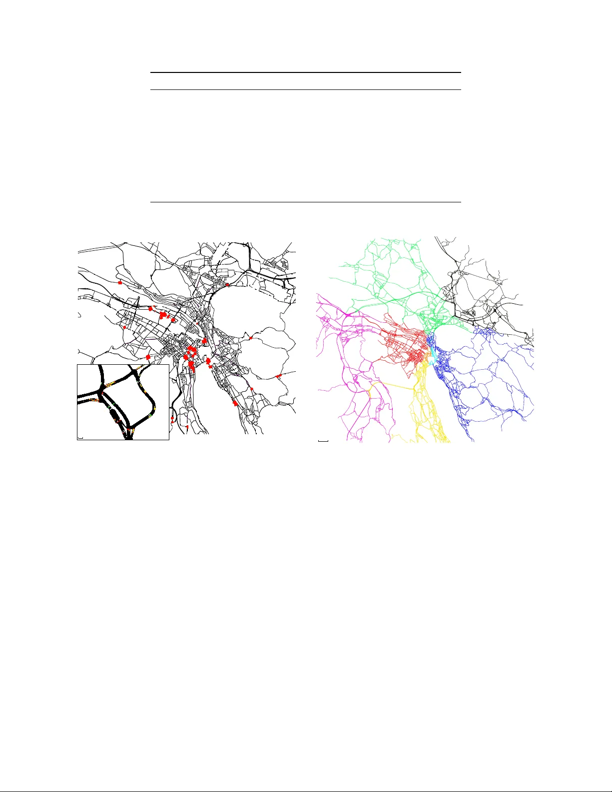
Data-driv en generalized p erimeter con trol: Züric h case study Alessio Rimoldi ∗ 1 , Carlo Cenedese 1,2 , Alb erto P adoan 3 , Florian Dörﬂer 1 , and John Lygeros 1 1 Automatic Con trol Lab oratory , ETH Züric h ( arimoldi,jlygeros,fdorfler@ethz.ch ) 2 Delft Cen ter for Systems and Control, TU Delft ( ccenedese@tudelft.nl ) 3 Dep. of Electrical and Computer Engineering, UBC ( alberto.padoan@ubc.ca ) F ebruary 28, 2026 Abstract Urban traﬃc congestion is a key challenge for the dev elopmen t of modern cities, requiring advanced control techniques to optimize existing infrastructures usage. Despite the extensive av ailabilit y of data, modeling such complex systems remains an expensive and time consuming step when designing model-based control approac hes. On the other hand, mac hine learning approaches require simulations to bo otstrap models, or are unable to deal with the sparse nature of traﬃc data and enforce hard constraints. W e prop ose a novel formulation of traﬃc dynamics based on behavioral systems theory and apply data-enabled predictive con trol to steer traﬃc dynamics via dynamic traﬃc light control. A high-ﬁdelit y simulation of the city of Zürich, the largest closed-lo op microscopic sim ulation of urban traﬃc in the literature to the best of our knowledge, is used to v alidate the performance of the proposed metho d in terms of total trav el time and CO 2 emissions. 1 In tro duction As cities worldwide grow at an ever-increasing pace, infrastructures struggle under the stress of increasing demand. The United Nations forecasts that b y 2050, 68% of the total world population will liv e in urban cen ters [ 1 ]. Roads remain by far the preferred mo de of transp ort for p eople and go ods b oth in the United States and the Europ ean Union [ 2 ], accounting for 74% of land freigh t transport in the European Union during 2021 [ 3 ]. The combination of these factors will mak e the problem of reducing urban traﬃc congestion ev en more challenging. Estimates show that road transp ort generates 12% of human CO 2 emissions and urban air p ollution has b een link ed to a host of negativ e health eﬀects [ 4 ]. T raﬃc congestion also leads to economic loss, due to unrealized productivity , v alued b et ween 1-2% of the Europ ean Union total gross domestic pro duct (80 to 160 billion euros p er y ear) [ 5 ]. Infrastructural c hanges aimed at solving this problem are limited in scale by prohibitive cost and their eﬀects are diﬃcult to predict due to counterin tuitiv e phenomena such as the Braess paradox [ 6 ]. F or this reason optimization of existing infrastructure through traﬃc management systems is often a preferable solution. A daptive traﬃc signal con trol is the most widespread form of urban traﬃc management [ 7 ], due to its eﬀec- tiv eness and relative low cost. The most common approac h is to deriv e a mo del of the city’s traﬃc dynamics and then apply mo del-based con trol algorithms suc h as Mo del Predictive Control (MPC) to compute opti- mal inputs for the traﬃc lights [ 8 ]. This metho dology w as pro ven to b e eﬀective [ 8 , 9 ] and easily in tegrates prior knowledge ab out the system into the mo del. Ho wev er, mo deling suc h large systems is expensive and ∗ This work was supp orted as a part of NCCR Automation, a National Center of Comp etence in Research, funded by the Swiss National Science F oundation (gran t num b er 51NF40_225155) A. Padoan ackno wledges the supp ort of the Natural Sciences and Engineering Research Council of Canada (NSERC). Grant num b ers: RGPIN-2025-06895 and DGECR-2025-00382 1 time consuming due to the dynamic large-scale nature of a cit y , where the road net work is often sub ject to c hanges (e.g., road closures) and demand changes ov er time. The av ailability of data is an opportunity to approac h the problem diﬀerently . Thanks to data-informed decision-making algorithms, it is now possible to iden tify and exploit complex patterns to eﬃciently con trol traﬃc. Data-driven metho ds are some of the most promising approaches when dealing with large-scale systems as they ha ve been shown to pro duce robust con trol policies without requiring explicit mo deling [ 10 – 12 ]. Current researc h in this area fo cuses on ma- c hine learning tec hniques, such as deep reinforcement learning, which hav e b een prov en to b e eﬀective when con trolling traﬃc systems [ 11 , 13 ]. T raining mo dels directly on traﬃc data can nonetheless b e challenging due to its sparse nature and the eﬀects of an input b eing delay ed in time. Deep reinforcemen t learning is kno wn to require large datasets to pro duce satisfactory p olicies. Synthetic data pro duced b y sim ulations can b e used, but this requires a mo del to simulate in the ﬁrst place. Recen tly , Data-enabled Predictive Con trol (DeePC) has b een applied to the Intersection T raﬃc Signal Con- trol Problem (ITSCP) showing promising results through Sim ulation-based Optimization (SimOpt) on a lattice netw ork [ 10 ]. This method has the adv antage of not needing an explicit model, as it bases its repre- sen tation of the traﬃc dynamics directly on data collected from the system, requiring less parameters and retaining higher in terpretability compared to machine learning procedures. Ev en though the ITSCP has b een a sub ject of research for ov er 70 y ears, there still exists a gap b et ween the literature and practical implementations [ 7 ]. One of the main reasons behind this gap is the lac k of a common b enc hmark in the ﬁeld. Most of the traﬃc researc h so far has fo cused on several diﬀerent small netw orks due to computational cost (see Section 1.1.6 ). These netw orks are often to o simple to allow conclusions to b e dra wn ab out real urban traﬃc netw orks and their diﬀerences make comparing diﬀerent approaches diﬃcult. With this in mind, this work builds on previous results [ 10 ], showing that solving the ITSCP via DeePC is a general approach able to handle large-scale netw orks and generic intersections. W e corrob orate our ﬁndings through closed-loop microscopic sim ulations based on the Simulation of Urban MObility (SUMO) pack age, using a real-scale high-ﬁdelit y sim ulation of the city of Züric h. 1.1 Literature Review The ITSCP is a complex problem inv olving many factors, suc h as h uman b eha vior, vehicle in teractions within the net work, sto c hastic traﬃc demand, and unpredictable even ts (e.g. traﬃc accidents). F or these reasons, it has b een the sub ject of extensive research since the seminal w ork in [ 14 ] and the developmen t of TRAﬃc Net work StudY T o ol (TRANSYT) [ 15 ]. In this section, we giv e a brief ov erview of the relev ant literature on traﬃc signal con trol, for a more in-depth o verview we refer the in terested reader to [ 7 , 16 , 17 ]. 1.1.1 Rule-Based Man y early approaches emplo yed rule-based metho ds to solv e the ITSCP. Rule-based metho ds work by deﬁning states and a set of appropriate actions asso ciated with each state to optimize a performance criterion. An example of these early metho ds can b e found in [ 18 – 20 ], where the authors dev elop ed the saturation ﬂo w algorithm. In [ 21 ] a rule-based algorithm is com bined with fuzzy logic. F uzzy rule-based systems deriv e actions from giv en inputs by deﬁning if-then rules whic h represen t the relationship betw een the v ariables [ 22 – 25 ]. In [ 26 ] the authors devise a dynamic rule-based system that changes the rules depending on traﬃc conditions to handle problems in real time. Ho wev er, as noted by [ 27 ], it can b e diﬃcult to generate eﬀectiv e rules, esp ecially for general in tersections with a large num b er of p ossible phases. 1.1.2 Dynamic Programming Dynamic programming has b een applied to the ITSCP to dev elop ﬂexible con trol algorithms applicable to a v ariety of traﬃc conditions. The authors of [ 28 ] ﬁrst applied dynamic programming using phases and stages as con trol v ariables. In [ 29 ] an algorithm based on dynamic programming capable of con trolling an arterial net work was dev elop ed. In [ 30 ] w as sho wn that an adaptiv e traﬃc signal con troller using appro ximate dynamic programming and reinforcement learning is capable of reducing vehicle delays. In [ 31 ], the authors 2 dev elop ed a recursiv e data pip eline comprising data processing, ﬂo w prediction, parameter optimization, and signal control. The main drawbac k of these metho ds is their computational complexity , which makes scaling to large scale urban traﬃc netw orks diﬃcult. Complexity can b e mitigated b y using techniques suc h as approximate dynamic programming at the exp ense of performance. 1.1.3 Distributed and Multi-Agent Metho ds Recen tly , there has been multiple attempts to con trol traﬃc net works in a distributed wa y [ 11 – 13 , 32 – 36 ]. A p opular distributed algorithm in traﬃc ligh t control is Max-pressure, deriv ed from the bac kpressure sc heduling framework [ 37 ]. The algorithm maximizes netw ork throughput by selecting, at each intersection, the phase with the largest upstream-downstream queue diﬀeren tial. The authors of [ 36 ] pro ved that a fully distributed implementation of Max-pressure stabilizes an y feasible demand distribution without requiring forecasts. In [ 35 ] the store-and-forw ard mo del is derived and the authors show that Max-pressure control is able to maximize the stabilit y region using only lo cal measurements and turn ratios. A practical dra wback of classical Max-pressure theory is that it ma y induce highly v ariable cycle lengths and rapid phase switc hing, moreo ver, it does not incentivize co ordination across the net work. Multi-agen t learning and game-theoretic approac hes are also used in this context. The authors of [ 32 ] w ere able to deal with computational c hallenges b y devising a distributed control approac h and tested it on a simulated 9 by 7 grid netw ork. The authors of [ 33 ] model an in tersection as a non-co operative game in whic h each play er (traﬃc signal) aims at minimizing its queue and the solution of the ITSCP is the Nash equilibrium of the game. In [ 11 – 13 , 34 ], the authors used reinforcemen t learning to implement co op erativ e hierarchical multi-agen t systems for real-time signal timing con trol of complex traﬃc net works. A drawbac k of these metho dologies is the inheren t diﬃcult y to pro vide theoretical guarantees such as stability or conv ergence. This is, ho wev er, a v ery activ e area of research. 1.1.4 Mo del Predictive Con trol MPC is a p ow erful con trol metho dology pro viding strong theoretical guarantees on the stability , feasibilit y , and optimality of the closed-lo op system, under the assumption of having a mo del that w ell describes the real system [ 38 ]. An example of its application to the ITSCP can b e found in [ 9 ], where a linear-parameter v arying form ulation of MPC for p erimeter ﬂo w control is presen ted. This line of w ork is based on the partitioning of the net w ork in to regions described b y the Macroscopic F undamental Diagram (MFD) [ 39 – 41 ]. In [ 42 ], a similar approach is presented using economic MPC and regional route-guidance actuation-based con trol. The authors in [ 43 ] prop ose tw o diﬀeren t macroscopic models of urban traﬃc to design an MPC algorithm able to compute a structured net work-wide traﬃc controller. These approaches are computationally eﬃcien t and allow for centralized con trol of large netw orks as sho wn in [ 9 ]. Ho wev er, mo del estimation pro cedures for such large systems can be computationally demanding. 1.1.5 Data-enabled Predictive Control Recen tly , there has b een a surge of interest for data-driven con trol approaches [ 44 ]. In this regard, b eha vioral system theory [ 45 ] oﬀers a p o werful tool to obtain systems descriptions directly from data. The main idea is that the set of all p ossible tra jectories of a dynamical system, called the b ehavior , con tains all the information necessary to describe the system. Beha viors of linear systems can be represen ted by non-parametrized models. F or linear systems, such representations are images of matrices containing data sampled from the system; these can then b e leveraged b y con trol algorithms. A particularly successful direct data-driv en con trol algorithm obtained in this wa y is DeePC [ 46 ], which has b een applied to numerous practical studies [ 46 – 48 ]. DeePC has b een also applied to urban traﬃc control, in the contexts of connected and autonomous vehicles co ordination [ 49 ] and v ehicle rebalancing in mobility-on-demand systems [ 50 ]. W e hav e previously sho wn DeePC to b e eﬀective in tackling the ITSCP on a symmetric lattice netw ork comprising 64 in tersections [ 10 ]. In this work we show that DeePC is suitable for con trolling m uch larger net works with general in tersection la youts. 1.1.6 Sim ulation-based Optimization SimOpt is a ﬁeld in which optimization tec hniques are in tegrated with simulation analysis [ 51 ]. Sim ulation to ols are frequen tly used in ITSCP research, approximately 77% of the pap ers in the ﬁeld use a sim ulation framew ork [ 17 ]. AIMSUN [ 52 ], CORSIM [ 53 ], MA TSim [ 54 ], Par amics [ 55 ], SUMO [ 56 ], VISSIM [ 57 ] 3 are some of the most widely used sim ulation pac k ages in research and industry . The ma jorit y of papers analyzed in [ 17 ] uses VISSIM as a simulation platform, closely follow ed b y SUMO. Most w orks focus on isolated single intersections [ 58 – 62 ] and regular lattice net works [ 63 – 67 ]. Some pap ers consider controlled roundab outs [ 68 , 69 ] and arterial netw orks [ 70 , 71 ]. In recent years, more general netw orks ha ve b een the fo cus of atten tion; for example, the authors of [ 72 ] considered a part of the city of Changsha, China as a simulation setting. In [ 73 – 75 ], the traﬃc netw orks of Skop je, Northern Macedonia; Bologna, Italy; and Lausanne, Switzerland w ere simulated. The largest online closed-lo op simulation, to the b est of the authors kno wledge is describ ed in [ 9 , 76 ] where a part of Barcelona, Spain is used as a net work, serving 79,143 v ehicles throughout the simulation. It is imp ortan t to note th at all these simulations mak e the unrealistic assumption that all intersections are four-legged intersections or do not regulate traﬃc ﬂo w at intersections; for example, [ 76 ] directly controls the ﬂows b etw een regions. 1.2 Con tributions The main con tributions of this pap er are three: (i) W e in tro duce a ﬂexible form ulation of the ITSCP based on b eha vioral theory that can seamlessly incorp orate diﬀerent kinds of data and generalize classical p erimeter con trol [ 8 ], the form ulation acco- mo dates other forms of actuation, suc h as dynamic sp eed limits, (ii) w e conjecture a linear relationship b et w een the traﬃc density and dynamic traﬃc light signals. W e v alidate this conjecture using extensiv e high-ﬁdelity simulations, (iii) w e p erform closed lo op con trol on what is, to the b est of our knowledge, the largest microsimulation in the literature equipp ed with demand estimated from real data. W e prop ose the simulation as a standard b enc hmark in traﬃc control research and use it to v alidate the performance of the prop osed metho dology in terms of trav el tim e and emissions metrics. The pap er is organized as follows. Section 2 describ es the metho dological framework, casting the ITSCP problem in the framework of b eha vioral system theory [ 77 ]. Section 3 presents the DeePC algorithm. Section 4 presents the sim ulation framework, the traﬃc netw orks used to test our metho d and numerical results sho wcasing the eﬀectiveness of the closed-loop con trol. Section 5 summarizes our ﬁndings and future research directions. Notation N denotes the set of p ositiv e integer num b ers, R , R n and R p × m denote the set of real num b ers, the set of n -dimensional vectors with real entries, and the set of p × m matrices with real entries, resp ectively . F or ev ery p ∈ N , the set of p ositiv e in tegers { 1 , 2 , ..., p } is denoted b y p . I denotes the identit y matrix. A map f from X to Y is denoted by f : X → Y ; ( Y ) X denotes the collection of all such maps. The restriction of f : X → Y to a set X ′ suc h that X ′ ∩ X  = ∅ is denoted b y f | X ′ and deﬁned as f | X ′ ( x ) = f ( x ) for x ∈ X ∩ X ′ . F or F ⊂ ( Y ) X , then F | X ′ denotes { f | X ′ : f ∈ F } . 2 Beha vioral form ulation of urban traﬃc dynamics 2.1 T raﬃc netw ork, sensing and demand W e consider the traﬃc netw ork of a city comp osed of intersections and roads, each divided into one or more lanes. F ollowing [ 42 ], we partition a city in p ∈ N regions of homogeneous av erage traﬃc densit y to leverage the concept of MFD, see Figure 6 . W e use the MFD to obtain a reference tra jectory for DeePC to track, as will b e discussed in Section 2.3 . Several metho ds can b e used to generate such a partitioning [ 78 ], here w e use a parallelized v ersion of the snake clustering algorithm [ 79 ], detailed in Appendix B . The algorithm ﬁnds connected clusters of roads with homogeneous av erage traﬃc density , yielding a low-scatter MFD. The set of resulting regions is deﬁned as p : = { 1 , · · · , p } . The most common sensors used by municipalities to measure traﬃc conditions are Eulerian sensors [ 80 ], whic h are stationary devices, as opp osed to L agr angian [ 81 ] sensors which can b e mobile. Throughout this 4 Figure 1: The cit y is divided into p regions homogeneous in av erage traﬃc density (the hexagons) and the demand d among them. A detail of sensors s j (blue diamonds) and traﬃc ligh ts l j (green circles) lo cations within region j ∈ p is sho wn. pap er, w e assume the use of Eulerian sensors, capable of measuring traﬃc densit y and ﬂow. Ho wev er, prop osed pro cedure is agnostic to the type of sensors used and Lagrangian sensors could b e in tegrated [ 82 ]. W e denote the set of sensors in region i ∈ p as s i : = { 1 , · · · , s i } , where s i ∈ N is the num b er of sensors in the region. F rom each sensor j ∈ s i , w e obtain the traﬃc densit y ρ j ( t ) [veh/km] and ﬂow ϕ j ( t ) [veh/h], at time t ∈ T ⊆ N , on the road where the sensor is lo cated, normalized by the n umber of lanes. W e then av erage the measuremen ts o ver each region i ∈ p , to reduce the v ariability and capture macroscopic v ariations [ 41 ]. W e denote the a verage density and ﬂow in region i ∈ p at time t ∈ T as ρ i ( t ) : = 1 s i s i X j =1 ρ j ( t ) (1a) ϕ i ( t ) : = 1 s i s i X j =1 ϕ j ( t ) (1b) The vectors of a verage densities and ﬂo ws in the city at time t are then, ρ ( t ) : = [ ρ i ( t )] p i =1 ∈ R p (2a) ϕ ( t ) : = [ ϕ i ( t )] p i =1 ∈ R p (2b) The evolution of ρ and ϕ dep ends on the ﬂow of vehicles en tering the traﬃc netw ork during every time in terv al, kno wn as the demand . The ﬂow of v ehicles starting their trip in region i ∈ p at time t with ﬁnal destination in region j ∈ p , is denoted by d ij ( t ) [v eh/h]; d ii ( t ) is the internal demand of region i , as seen in Figure 1 . The vector of demands starting in region i is denoted b y d i ( t ) : = [ d ij ( t )] p j =1 ∈ R p , while the 5 v ector of all the demands among all regions is d ( t ) : = [ d i ( t )] p i =1 ∈ R p 2 . Despite b eing inﬂuenced by many factors such as comm uters c hoices and weather conditions, d ( t ) presents seasonal patterns at diﬀeren t time scales, w eekly , mon thly , and yearly , that make it p ossible to reliably estimate it [ 83 ]. Demand estimation, in the form of time dep endent origin-destination pairs, is a well-kno wn problem and has b een extensively studied [ 84 , 85 ]. In this w ork, we do not consider the problem of predicting the demand and instead w e consider it as a given exogenous input to the system. 2.2 In tersection Control F ollowing [ 7 ], we deﬁne an interse ction as a set of appr o aches and a cr ossing ar e a . The cr ossing ar e a is the p ortion of space delimited by the stop lines of the approaches, where vehicles and pede strians are allo wed to cross intermitten tly under right of w ay . An appr o ach is a road leading to the crossing area, comprising one or more lanes , each equipped with a signal he ad . Signal heads can be in one of three states: gr e en (g), yel low (y), or r e d (r); the set of all the signal heads in the in tersection makes up the tr aﬃc signal of the intersection. Approac hes are used by tr aﬃc ﬂows to reach the crossing area. T wo ﬂows are said to b e c omp atible when the vehicles composing them can pass the crossing area sim ultaneously under right of wa y; otherwise they are called antagonistic . Figure 2 sho ws a simpliﬁed dra wing of an in tersection. On the left the crossing area, approac h, lane and signal heads are highligh ted for clarit y . On the righ t the diﬀerence b et ween compatible and antagonistic ﬂows can b e seen. Crossing area Lane Approac h Signal head Compatible ﬂows An tagonistic ﬂo ws Figure 2: Example of a four-legged intersection and compatibilit y of traﬃc ﬂows. On the left the structural comp onen ts of the intersection are highligh ted for clarit y . On the righ t the diﬀerence b etw een compatible and antagonistic ﬂows can b e observed. A traﬃc signal duty cycle , is an ordered set Π of phases , its duration is called cycle time ∆ dc . A phase is a tuple containing the state v alue for each signal head, and is designed to allow compatible traﬃc ﬂows to cross the in tersection. Figure 3 illustrates a duty cycle for a four legged in tersection, where a phase of only red states is used to clear the intersection. By inﬂuencing the ﬂow of vehicles trav eling through an actuated intersection, it is p ossible to indirectly inﬂuence ϕ i ( t ) and ρ i ( t ) . Given tw o regions i, j ∈ p , if one in tersection sitting at the b oundery b et ween i and j can be actuated, one can regulate the ﬂow of v ehicles moving b et ween the tw o regions at that p oint. If one can con trol all the access points from region i to j , then the ﬂow of v ehicles moving b et ween the t wo regions can b e directly controlled, that is, classical p erimeter control [ 42 ]. Remark ably , our approach do es not assume the actuators to b e placed at the b oundaries of the regions, as this is rarely the case in practice. Instead, we allo w the actuators to b e placed anywhere within the netw ork, see Figure 1 . According to [ 7 ], there are four p ossible approaches when controlling traﬃc light op erations: 6 I: {g,g,r,r,g,g,r,r} I I: {y ,y ,r,r,y ,y ,r,r} I II: {r,r,r,r,r,r,r,r} IV: {r,r,g,g,r,r,g,g} V: {r,r,y ,y ,r,r,y ,y} VI: {r,r,r,r,r,r,r,r} Figure 3: Example of a duty cycle comprising six phases divided in active and passiv e. Activ e phases (I,IV) are group ed in the leftmost column and highligh ted in green, while passive phases (I I,I II,V,VI) can b e found in the t wo rightmost columns highlighted in red. Activ e phases ha ve at least one ’g’ state in the tuple. • Phase sp e ciﬁc ation : The control input is the state comp osition of the phases. When dealing with complex intersections in volving a multiple approaches, the speciﬁcation of the optimal composition of the phases is non-trivial and has a ma jor impact on the in tersection’s eﬃciency , often giving rise to mixed-in teger problems [ 86 ]. • Split c ontr ol : The control input is the duration of each phase as a p ortion of the duty cycle time ∆ dc . This duration can b e optimized based on current netw ork conditions. • Cycle time : The con trol input is the cycle time ∆ dc . Longer cycle times lead to an increase in eﬃciency due to the smaller proportion that the constant lost times o ccup y , how ever, this may increase v ehicle dela ys in underutilized intersections due to the longer red phase. • Oﬀset : The control input is the phase diﬀerence b et ween the dut y cycles of multiple successive inter- sections. In contrast to previous schemes, this approach assumes multiple in tersections to b e actuated. This can be used, for example, to generate a gr e en wave along an arterial. In this work, w e fo cus on split c ontr ol with ﬁxed duty cycle time ∆ dc , making our metho d a ﬁxed-time adaptiv e strategy in the classiﬁcation of [ 7 ]. Under this scheme, the optimization problem can b e readily form ulated as a quadratic program with contin uous b ounded inputs. This problem can b e solved eﬃciently , enabling practical implemen tations where the resp onse time of the system is constrained. W e consider the Split c ontr ol sc heme with ﬁxed duty cycle time ∆ dc for each controlled intersection. The actuated intersections are acting under the co ordination of a cen tralized controller. The dut y cycle of ℓ -th actuated in tersection, is a ﬁnite ordered set Π ℓ whose elemen ts are referred to as phases . Given an intersection with n approaches eac h equipp ed with a signal head that can b e red (r), yello w (y) or green (g) for any time in terv al, w e deﬁne a phase as the n -tuple y ∈ { r , y , g } n , where the i -th element represents the state of the i -th signal head. W e associate to each phase i ∈ Π ℓ a duration δ i ∈ N in seconds and we deﬁne the duty 7 cycle time ∆ ℓ dc ∈ N as ∆ ℓ dc = X i ∈ Π ℓ δ i . When a phase con tains at least one ’g’ v alue we call it an active phase ; otherwise, we call it a p assive phase . Note that w e include the duration of y ellow phases in the duration of passiv e phases, see Figure 3 . The set of active phases for the ℓ -th traﬃc ligh t is denoted as A ℓ ⊂ Π ℓ , the set of passive phases corresponds to A c ℓ . In tuitively , the main diﬀerence b et ween an active phase and a passiv e one is that during an activ e phase, some vehicles are allo wed to cross the in tersection. The duration of the active and p assive phases are δ a = X i ∈A ℓ δ i , and δ p = X i ∈A c ℓ δ i = ∆ ℓ dc − δ a , resp ectiv ely . W e deﬁne the p ercen tage of time, with respect to the duty cycle time, for which an in tersection is active as λ ℓ = δ a / ∆ ℓ dc ∈ [0 , 1) , 0 ≤ δ a ≤ ∆ ℓ dc . By con trolling the v alue λ ℓ one con trols the fraction of ∆ dc for whic h the intersection is active, where a v alue λ ℓ ( t ) = 0 corresp onds to an intersection with all the signal heads red for the whole dut y cycle. Note that while the v alue λ ℓ ( t ) = 0 is achiev able, the v alue λ ℓ ( t ) = 1 is not due to the constan t duration of the yello w phases em b edded in the passiv e phase duration. F or the sake of simplicit y , we consider the v alues λ ℓ ( t ) to b e real n umbers, and w e recov er the corresp onding δ a b y means of a ﬂo or op eration. Figure 4 sho ws an example of input tra jectory and for the ℓ -th traﬃc light and the resulting v alues of δ a and δ p . δ p δ a ∆ dc 2∆ dc 3∆ dc λ ℓ ( k ) 0 1 ∆ dc 2∆ dc 3∆ dc Figure 4: Diﬀeren t con trol input v alues λ ℓ result in diﬀeren t active and passive phase durations, that is δ a and δ p , for a traﬃc light ℓ ∈ l . The b ottom graph shows a p ossible input tra jectory for the ℓ -th traﬃc ligh t spanning three duty cycles, the top graph shows prop ortion of dut y cycle time assigned to the active and passiv e phases as a result of the input. W e deﬁne the con trol input giv en to our system at time t as the vector λ ( t ) : = [ λ i ( t )] l i =1 ∈ R l , with l : = { 1 , · · · , l } denoting all the actuated traﬃc ligh ts. This form ulation allows one to control a general in tersection with a single scalar b ounded input λ ℓ ( t ) . How ever, it comes with the disadv antage of relinquishing control o ver the durations of the individual phases, which determine traﬃc ﬂo ws with diﬀeren t directionalities. T o mitigate this shortcoming, one could introduce additional inputs to distinguish b et ween diﬀerent phases, at the cost of a more computationally exp ensive optimization problem. W e assume that the traﬃc demand on one side of the intersection has greater magnitude than the opposite direction, which is often the case during p eak hours. Under this assumption, the con trol input λ ℓ ( t ) is suﬃcien t to decongest the intersection. 2.3 Macroscopic fundamen tal diagram The concept of MFD captures the relation b etw een the ﬂow ϕ i and densit y ρ i within a region i ∈ p . F or eac h region i ∈ p w e plot the measuremen ts of ( ρ i , ϕ i ) against eac h other and estimate the MFD using a 4-th degree p olynomial, see Figure 6 . W e then use the estimated MFD to identify eac h region’s critical density and maximal densit y , denoted as ρ cr ,i , and ρ max ,i , resp ectiv ely . The critical densit y ρ cr ,i corresp onds to the 8 abscissa of the maximum point for the MFD of region i , where the region reac hes its maximum p ossible ﬂo w and throughput. This observ ation will b e used later in Section 3 to deﬁne the reference tra jectory to b e trac ked. W e deﬁne the v ector of critical densities as ρ cr : = [ ρ cr ,i ] p i =1 ∈ R p . The maximal density ρ max ,i is the smallest p ositiv e ro ot of the p olynomial used to estimate the MFD, where the netw ork reaches its maximum capacit y and the ﬂow equals zero. This state is often referred to as grid-lo c k, and we deﬁne the v ector of the maximal densities as ρ max : = [ ρ max ,i ] p i =1 ∈ R p . The MFD c aptures the non-linear and non-injective relation that exists b et ween the density ρ i and ﬂow ϕ i in each region i ∈ p . As we will discuss in Section 3 , DeePC works best under an approximately linear relationship b et ween the input and output measurements of the system. Despite the non-linear dependencies enco ding the system dynamics through the MFD, as sho wn in Section 4 and supp orted by [ 10 ], the DeePC algorithm is able to ﬁnd eﬀective control p olicies using λ as the control input and ρ as the output measure- men t. This observ ation leads us to conjecture that the relationship betw een the input λ and the densit y ρ m ust b e appro ximately linear. Moreo ver, empirical trials conducted by the authors using only the ﬂow ϕ or a combination of ﬂow and density y ( t ) := col ( ϕ ( t ) , ρ ( t )) as output of the system resulted in degraded p erformance of the algorithm (data not shown). This mak es us conjecture that the relationship b et ween λ and ϕ m ust b e non-linear, a fact that is not surprising giv en the non-linear relationship b et ween densit y and ﬂo w. The t wo conjectures are summarised in the commutativ e diagram in Figure 5 . λ ρ ϕ appro x. linear non-linear non-linear non-injectiv e Figure 5: Commutativ e diagram of the relationships betw een λ , ρ and ϕ . The relationship b etw een ρ and ϕ is assumed to b e a MFD similar to Figure 6 . 2.4 Beha vioral traﬃc dynamics W e mo del traﬃc as a dynamical system using behavioral system theory [ 45 , 87 , 88 ]. The resulting form ula- tion naturally generalizes p erimeter traﬃc control by allowing the actuators to b e placed an ywhere in the net work. A b ehavioral form ulation is ﬂexible, as it can in principle integrate any kind of measurement data. F or example, in a traﬃc system, one could consider CO 2 emissions or noise as alternative outputs of the system. Below we give a brief in tro duction to b eha vioral systems theory , the interested reader is referred to App endix A for more details. In b eha vioral systems theory a dynamic al system (or, brieﬂy , system ) is a triple Σ = ( T , W , B ) [ 45 ], where T is the time set , W is the signal set , and B ⊆ ( W ) T is the b ehavior of the system. The behavior characterises the set of all signal tra jectories ov er the time set T that are compatible with the system. More sp eciﬁcally , if the signal set is W = R q the set of ﬁnite tra jectories w = ( w (1) , . . . , w ( T )) of length T ∈ N , with w ( t ) ∈ W for t ∈ T : = [1 , . . . , T ] ⊂ N , is W T = ( R q ) T and the b eha vior is a subset B ⊆ ( R q ) T . W e iden tify every ﬁnite tra jectory w ∈ ( R q ) T with the corresp onding v ector col( w (1) , . . . , w ( T )) ∈ R q T . In this case, a system Σ is called line ar if the corresp onding b eha vior B is a linear subspace, and time-invariant if B is shift-inv ariant, i.e. , if w ∈ B implies σ w ∈ B , where σ is the shift op er ator deﬁned as ( σ w )( t ) : = w ( t + 1) . The class of all complete Linear Time-Inv arian t (L TI) systems is denoted by L q , and for simplicity we write B ∈ L q to denote a linear b eha vior. 9 0 10 20 30 40 50 60 70 80 90 100 0 50 100 150 200 250 ρ cr ,i ρ max ,i ρ i ϕ i Data MFD Figure 6: The MFD for the region of Wiedikon, Zürich (solid green line) simulated b elo w. The critical densit y ρ cr ,i is the densit y where the ﬂow is maximum, and the maximal density of region ρ max ,i is the densit y where the ﬂow b ecomes zero and region i gridlo c ks. T o mo del the traﬃc dynamics outlined ab o ve in this framework, we consider b eha viors B ∈ L m + p o ver a signal w = col( u, y ) ∈ R q divided into an input u of dimension m = l + p 2 and an output y of dimension p . As output w e consider the traﬃc densit y ρ ∈ R p in the p regions of the traﬃc netw ork. The inputs u are further sub divided into con trollable inputs λ ∈ R l (the fractions of activ e phase of the controlled intersections) and uncon trollable inputs d ∈ R p 2 (the demands of all p ossible origin-destination region pairs). This leads to u ( t ) : = col( λ ( t ) , d ( t )) ∈ R m , y ( t ) : = ρ ( t ) ∈ R p , and a signal w = col( u, y ) ∈ R q of dimension q = l + p + p 2 . The dynamics of the signal are describ ed by a non-linear function h relating, for example, the densit y or ﬂow in one time instant with those in the next time instan t. Common choices for h include partial diﬀeren tial equations, discretised b y ﬁrst or second order metho ds [ 89 , 90 ]. In this work, we do not concern ourselves with the c hoice of a sp eciﬁc mo del for h , but consider tra jectories of the corresponding quantities and construct a high-dimensional linear approximation f of h based solely on data. Let T , T ini ∈ N with T ini < T and a ﬁxed t ∈ T , consider a ﬁnite output tra jectory y | [ t − T ini ,t ] = ( y ( t − T ini ) , . . . , y ( t )) , and input tra jectory u | [ t − T ini ,t ] = ( u ( t − T ini ) , . . . , u ( t )) . W e then consider a linear function f : ( R p ) T ini × ( R m ) T ini → R p of the follo wing form y ( t + 1) = f ( y | [ t − T ini ,t ] , u | [ t − T ini ,t ] ) , (3) and introduce the b eha vior asso ciated with the traﬃc density as B ρ = n ( y , u ) ∈ R ( l + p + p 2 ) T ini | ( 3 ) holds o . (4) Note that in what follows we never explicitly construct the b eha vior in 4 , but enco de the constraint in 3 implicitly using data collected from the system. T o ensure that the tra jectories included in the behavior are realistic, additional constrain ts need to be imp osed. Let T f ∈ N be a multiple of the duty cycle time ∆ dc and such that T ini + T f ≤ T . W e assume that 10 once the input λ has b een chosen, it is kept constan t during the duty cycle, that is for a duration ∆ dc . This translates in to the linear constraint M u = 0 , where M ∈ R mT f × mT f is used to imp ose for ev ery ℓ ∈ l and k ≤ T f the constrain t λ ℓ ( k + 1) = λ ℓ ( k + 2) = · · · = λ ℓ ( k + ∆ dc ) . W e further assume that at every time instan t the con trollable input has to satisfy the b o x constraints λ ( k ) ∈ [ λ , λ ] ⊂ [0 , 1) l , where λ = col( λ 1 , · · · , λ l ) and λ col( λ 1 , · · · , λ l ) As mentioned b efore, the v alues are not allo wed to reach the boundary v alue 1 due to the yello w phase constan t duration. The uncontrollable input d is assumed to b e known and equal to an estimate of the demand d = col(( d ( t ) , · · · , d ( t + T f ))) ∈ R p 2 T f o ver the prediction horizon, i.e., D u = d where the matrix D ∈ R mT f × p 2 T f pro jects to the en tries of the input corresp onding to the demand. Therefore, the set of constrain ts for the inputs o ver the whole prediction horizon reads as U = n u ∈  [ λ , λ ] × R p 2 +  T f | M u = 0 , D u = d o . (5) Similarly , b ox constrain ts on the output are selected to ensure that the density remains non negativ e and b elo w grid-lo c k conditions ρ max ∈ R p + , leading to y ( t ) ∈ [0 , ρ max ] and a constrain t set Y : = [0 , ρ max ] T f . 3 Data-enabled predictiv e con trol Consider a L TI system B ∈ L m + p , with m inputs and p outputs, assume that data recorded oﬄine from system B is av ailable. Sp eciﬁcally , assume that an input sequence u d = col( u d (1) , · · · , u d ( T )) ∈ R mT of given length T ∈ N is applied to the system B and that the corresp onding output sequence y d = col( y d (1) , · · · , y d ( T )) ∈ R pT is recorded. The subscript “ d” is used to indicate that these are tra jectories of data samples collected oﬄine. Finally , let T ini ∈ N and T f ∈ N , with T ini + T f ≤ T , and assume that the sequence w d = col( u d ( t ) , y d ( t )) ∈ R ( m + p ) T , for t ∈ T : = [1 , . . . , T ] ⊂ N , satisﬁes the generalized p ersistency of excitation condition (see App endix A ). Intuitiv ely , the p ersistency of excitation condition requires the sequence w d to contain enough information to allo w for the systems’ b eha vior to be reconstructed. W e deﬁne the Hankel matrix of depth L ∈ T asso ciated with the ﬁnite sequence w ∈ R q T as H L ( w ) =      w (1) w (2) · · · w ( T − L + 1) w (2) w (3) · · · w ( T − L + 2) . . . . . . . . . . . . w ( L ) w ( L + 1) · · · w ( T )      . Next, we partition the input-output data into tw o parts, p ast data ( U p , Y p ) and futur e data ( U f , Y f ) . F ormally , giv en the time horizons T ini ∈ N and T f ∈ N , w e deﬁne  U p U f  = H T ini + T f ( u d ) ,  Y p Y f  = H T ini + T f ( y d ) , (6) where U p ∈ R ( mT ini ) × ( T − T ini +1) is composed of the ﬁrst T ini blo c k-ro ws of the matrix H T ini + T f ( u d ) and U f ∈ R ( mT f ) × ( T − T f +1) of the last T f blo c k-ro ws, Y p and Y f are attained similarly from H T ini + T f ( y d ) . In the remainder, past data, denoted b y the subscript “ p ”, is used to implicitly estimate the initial condition of the underlying state, whereas the future data, denoted b y the subscript “ f ”, is used to predict future tra jectories. Giv en T f ∈ N , a reference tra jectory for the output ˆ y and the input ˆ u , most recent past input/output data w ini = col( u ini , y ini ) , an input constrain t set U ⊆ R mT f , an output constrain t set Y ⊆ R pT f , an output cost matrix Q ≥ 0 ∈ R p × p , a control cost matrix R ≥ 0 ∈ R m × m , a regularization function ψ : R T − T ini − T f +1 → R , and parameters λ y , λ 1 , λ 2 ∈ R , the DeePC algorithm solves the optimisation problem: 11 min u,y ,g,σ y T f X k =1 ∥ y ( k ) − ˆ y ( t + k ) ∥ 2 Q + ∥ u ( k ) − ˆ u ( t + k ) ∥ 2 R + ψ ( g ) + λ y ∥ σ y ∥ 1 (7a) s.t.     U p Y p U f Y f     g =     u ini y ini u y     +     0 σ y 0 0     , (7b) u ∈ U , y ∈ Y . (7c) Solving ( 7 ) generates a tra jectory of future inputs , u , and outputs, y , for the next T f time steps. The equalit y constrain t ensures that the tra jectories are compatible with the system dynamics (enco ded in the data matrix) and the most recen t data collected from the system and stored in u ini and y ini . The regularization term ψ ( g ) is deﬁned as ψ ( g ) := λ 1 || ( I − Π) g || 2 2 + λ 2 || g || 1 where Π =   U p Y p U f   †   U p Y p U f   . The ﬁrst addend || ( I − Π) g || 2 2 computes the orthogonal pro jection on the kernel of the ﬁrst three blo ck equations of ( 7b ), while the second added || g || 1 computes a low-rank approximation on the column space of H . T ogether the tw o terms greatly improv e the performance of DeePC in non-linear settings, for more details on the regularization action the in terested reader is referred to [ 91 ]. The slack v ariable σ y relaxes the constrain t to ensure that it remains feasible; it is p enalised by the regularization term λ y || σ y || 1 to keep the constrain t violation small. The set membership constrain ts ( 7c ) ensure that the decision v ariables remain within the admissible input domain U and the physically consistent output domain Y . The cost ( 7a ) trades oﬀ tracking accuracy || y ( k ) − ˆ y ( t + k ) || 2 Q and control eﬀort || u ( k ) − ˆ u ( t + k ) || 2 R with resp ect to the reference v alues ˆ y and ˆ u . Once th e optimisation problem is solved, the ﬁrst element of the tra jectory u is applied to the system, a new measuremen t is collected, the vectors u ini and y ini are up dated with this new information and the process is rep eated in a receding horizon fashion. The pro cess is summarised in Algorithm 1 . Algorithm 1 DeePC Input: F uture time horizon T f ∈ N , a reference tra jectory for the output ˆ y = ( ˆ y 0 , ˆ y 1 , · · · ) ∈ ( R p ) N and the input ˆ u = ( ˆ u 0 , ˆ u 1 , · · · ) ∈ ( R m ) N , past input/output data w ini = col( u ini , y ini ) ∈ B | [1 ,T ini ] , an in- put constrain t set U ⊆ R mT f , an output constrain t set Y ⊆ R pT f , a output cost matrix Q ∈ R p × p , a control cost matrix R ∈ R m × m , a regularization function ψ : R T − T ini − T f +1 → R , and parameter λ y ∈ R . 1: Compute the minimizer g ∗ of ( 7 ). 2: Compute optimal input sequence u ⋆ = U f g ⋆ . 3: Apply optimal input sequence ( u t , · · · , u t + j − 1 ) = ( u ⋆ 1 , · · · , u ⋆ j ) for some j ≤ T f . 4: Set t to t + j and up date u ini and y ini to the T ini most recent input/output measuremen ts. 5: Return to 1 . F or our traﬃc mo del we use the quantit y ρ cr estimated from the regions MFDs in Section 2.3 as constan t output reference ˆ y . In ( 7 ), we minimize the distance betw een the regions’ density ρ i and critical ρ cr ,i at eac h time step. The MFD (and hence the reference ˆ y ) can initially b e estimated using data from the historical op eration of the system. W e note, how ev er, that this data implicitly dep ends on the policy used to control the in tersections. Since our goal is to change this p olicy , it is conceiv able that when the system is op erating under the DeePC algorithm, its MFD will c hange. This eﬀect can b e mitigated b y re-estimating the MFD online with data collected under the DeePC p olicy , the reference ˆ y can be recomputed and the process rep eated. One should b e careful to ensure the stability of the algorithm as considering a non-contin uous 12 tra jectory can be problematic. F or the sake of a fair comparison among the diﬀeren t control p olicies explored in Section 4 , w e decided to leav e this online optimization of the control scheme for future researc h. The reference v alue of the inputs ˆ u := col( ˆ λ, ˆ d ) is comp osed b y t w o parts, the ﬁrst is the default green time to dut y cycle time ratio ˆ λ , which is the ratio that the traﬃc lights w ould exhibit given their phase sp eciﬁcation if no dynamic control were to b e applied. The latter is exogenous and set equal to d according to ( 5 ). In the cost function in ( 7 ), the matrices R and Q are chosen p ositiv e deﬁnite. Note that the comp onen ts of ∥ u − ˆ u ∥ R asso ciated w ith d are alw ays equal to zero due to the chosen reference and the constrain ts on u . Finally , the regularization term ψ is chosen as in [ 46 ]. Note that in general the optimization problem only requires conv exity of the cost function. 4 Sim ulation W e use SUMO to sim ulate traﬃc dynamics at a microscopic lev el and generate realistic data. An im- plemen tation of the controller then interacts with the simulation in closed-lo op through a custom in- terface built on T raCI. The interface code as w ell as the simulations net works are op enly a v ailable at https://github.com/AlessioRimoldi/TrafficGym . The routing of each v ehicle is recomputed p eriodically using the A* algorithm, accounting for current traﬃc conditions. Once a v ehicle reaches its destination, it is remov ed from the sim ulation. W e consider tw o diﬀerent traﬃc netw orks, a lattice netw ork and the urban traﬃc netw ork of Züric h. W e use a sim ulation where the traﬃc lights follow the standard static cycle sp ec- iﬁed b y the SUMO conﬁguration as a baseline, in this case no input is giv en to the simulation. W e further compare DeePC with the MPC formulation detailed in [ 76 ], in this work the authors ﬁrst devise a linear program form ulation to solve the ﬁnite-time optimal perimeter ﬂow con trol problem. The traﬃc dynamics are described ﬁrst using a non-linear mo del deriv ed from the MFD, the linear form ulation is then achiev ed as a linearization of this model, employing a piecewise approximation of the MFD. The linear program is then solved in a rolling horizon using a feedback MPC framework, for completeness we rep ort the MPC form ulation in App endix C . The parameters used by the controllers can b e found in Appendix D . 4.1 Lattice net work sim ulation The lattice netw ork is comp osed of 104 t wo-w ay roads and 64 in tersections. Figure 7b shows the net work partitioned in to t wo regions em ulating a cit y cen ter and its suburban area, connected b y 8 roads. W e refer to these t wo regions as the inner and outer region respectively . A ctuators and demand proﬁle W e selected t welv e traﬃc lights to be used as actuators, eight of which are at the boundary b etw een the tw o regions and can b e used to p erform classical p erimeter con trol, while the remaining are in the inner region to manage the in ternal dynamics, see Figure 7b . All controlled in tersections ha ve four approac hes. W e consider a standard dut y cycle time of ∆ dc = 90 s , with tw o green phases lasting 42 seconds, plus tw o yello w phases lasting 3 seconds. The demand proﬁle in Figure 7a has t wo distinct p eaks, spanning tw o hours with a total of 6149 v ehicles. Each v ehicle is generated at the external boundary of the outer region, and assigned a destination edge inside the inner region. This makes the demand unidirectional, from the outer to the inner region, no additional v ehicles are generated. Results The evolution of the density and ﬂow in the inner region is shown in Figure 8 . The baseline sim ulation reaches a state of grid-lo c k shortly b efore the end of the ﬁrst p eak of demand, leading to high tra vel times. Due to the congestion only 4636 v ehicles complete their trip. On the other hand, con trol of the traﬃc ligh ts via DeePC and MPC prev ents grid-lo c k, main taining a stable ﬂo w throughout the length of the simulation. T able 1 sho ws the av erage tra vel time and emissions metrics o ver the n umber of vehicles that completed their trip, w e observe DeePC p erforming b etter than MPC on all metrics. W e conjecture that this impro vemen t in p erformance is due to the implicit mo del deﬁned b y the Hankel matrix included in DeePC capturing the underlying traﬃc dynamics b etter than the linear formulation used by MPC, note that b oth mo dels p erform a linear appro ximation. 13 0 20 40 60 80 100 120 20 40 60 80 100 Time (min) Demand (veh/min) (a) 100 m (b) Figure 7: Left panel shows the demand proﬁle, the vehicles mo ve from the outer to the inner region. The net work is partitioned into the outer r e gion (solid magen ta line) and in inner r e gion (dashed green line). Blac k dots represent the con trolled traﬃc ligh ts. 0 20 40 60 80 100 120 0 10 20 30 40 Time (min) ρ (veh/km) DeePC MPC Baseline (a) 0 20 40 60 80 100 120 0 50 100 150 Time (min) ϕ (veh/h) DeePC MPC Baseline (b) Figure 8: Evolution of the densit y (left panel) and ﬂow (right panel) in inner region of the lattice net work. 4.2 Züric h simulation W e now present the sim ulation of Züric h, Switzerland, built on a digital twin developed at T ranscality [ 92 ]. The urban traﬃc net work of the cit y comprises almost 15,000 roads with diﬀerent num b er of lanes, connecting appro ximately 7,000 intersections, see Figure 9 . The demand proﬁle is estimated using real data measured b y the city lo op detectors. In our exp erimen ts, we consider the p eriod corresp onding to the ev ening traﬃc p eak, spanning the hours from 16:00 to 21:00. During this surge in demand, the net work serves more than 170,000 vehicles. Figure 9b shows the traﬃc regions obtained by applying a parallelized version of the snake clustering algorithm describ ed in [ 79 ], see App endix B . Remark ably , the iden tiﬁed regions closely resemble the real districts of the city , for example, one can recognize the Wiedikon area in red. This similarity is due to the use of real data in demand and traﬃc netw ork mo deling. 14 Baseline MPC DeePC % v ariation T rav el Time (min) 27.5 26.03 24 . 93 - 9.34% W aiting Time (min) 25.33 22.24 21 . 39 - 15.55% CO Emissions(g) 259.65 239.59 229 . 5 - 10.92% CO2 Emissions (g) 4,351.16 4,084.12 3 , 917 . 79 - 9.95% HC Emissions (g) 1.28 1.19 1 . 14 - 10.37% PMx Emissions (g) 0.11 0 . 1 0 . 1 - 8.95% NOx Emissions (g) 1.98 1.86 1 . 78 - 10.10% F uel consumption (ml) 1,387.91 1,302.73 1 , 249 . 67 - 9.96% T rips completed 4,636 5,377 5 , 642 + 21.69% T able 1: A v erage metrics for the lattice netw ork 0 1000m 0 10m (a) 0 1000m (b) Figure 9: Left panel shows the Zürich urban traﬃc netw ork embedded in SUMO. Actuated in tersections are highligh ted in red. In the corner, one of the controlled intersections, Bellevue. Right panel shows the region partitioning found using the snake clustering algorithm, the Wiedik on region is highlighted in red. A ctuators and demand proﬁle The net work comprises ov er 800 intersections with controllable traﬃc ligh ts. T o ensure the sim ulation is realistic, we took adv an tage of the exp ert kno wledge of the traﬃc engineers of the cit y of Zürich and selected the 47 actuators that the municipalit y is currently using as actuators [ 93 ], the p osition of these actuators can b e seen in Figure 9a . Although the phase deﬁnition dep ends on the top ology of the intersection, all actuated traﬃc lights ha ve a duty cycle time of ∆ dc = 72 s . One of the actuated in tersections can be seen in Figure 9a . The demand proﬁle directed to the Wiedikon region (highligh ted in red in Figure 9b ) is sho wn in Figure 10 , where the color co ding of the plot matches the one of Figure 9b . The data is collected during a day of a verage congestion in the cit y , therefore the baseline sim ulation do es not reach a grid-lo c k. Results The comparison of densit y and ﬂo w under control of DeePC and MPC for the Wiedik on region, highligh ted in red in Figure 9b , can b e seen in Figure 11 . Figure 11a additionally sho ws the v alue of the critical densit y ρ cr of the region. Due to the high v ariability of the ﬂo w, a mo ving av erage ﬁlter of windo w 15 20 40 60 80 100 120 140 160 180 200 220 240 260 280 300 0 20 40 60 80 100 Time (min) d (veh/min) Oerlikon Wiedik on Züriberg Uetliberg Enge Opﬁkon Center 1 Cen ter 2 Figure 10: The demand proﬁle directed to the Wiedik on region broken down by region of origin. The color co ding used matc hes the one in Figure 9b . 10 has b een applied to the ﬂow time series to aid comprehension of plot 11b . The behavior of this region is represen tative as all the other regions in the net work behav e similarly . Also in this netw ork DeePC is able to outp erform MPC and improv e traﬃc conditions leading to a 18% decrease in trav el time, see T able 2 . This suggests that the data-generated approximation of the relation b et ween traﬃc light control and densit y succeeds in capturing traﬃc dynamics eﬀectively . This supp orts the conjecture made in Figure 5 that the relation b et ween the t wo quantities is linear. The MPC controller also achiev es an improv ement in trav el time which, ho wev er, remains higher than under the DeePC p olicy . One reason for this is that the MPC solv es the p erimeter con trol problem by computing the optimal ﬂows, referring back to Figure 5 , we know that the relation b etw een the traﬃc light control and the ﬂow to b e non-linear, this leads to an inaccurate linear approximation. Moreo ver, b oth algorithms p erform a linearization of the traﬃc dynamics providing a fair comparison, how ever, since the MPC formulation computes ﬁrst the optimal ﬂo ws b etw een regions, a mapping b et ween these ﬂows and the actuators is then needed to assign the inputs to the right actuators. If the actuators are placed on the borders b et ween regions constructing this mapping is trivial. If, ho wev er, the actuators are allow ed to b e anywhere in the netw ork, this makes constructing the mapping more diﬃcult, as one actuator could b e resp onsible for the mo dulation of multiple ﬂows directed to diﬀerent regions. In practice, each actuator must receive just one input at a time, this requires it to b e assigned to a single ﬂo w whic h introduces an approximation error and degrade p erformance. DeePC a voids this problem as the mapping is deﬁned implicitly by the Hank el matrix leading to b etter p erformance. Because up dating the con trol at ev ery dut y cycle may b e undesirable in practice due to the frequent changes in phase duration, w e also ev aluate DeePC with longer control p eriods. Sp eciﬁcally , we sim ulate con trol with a p eriod of 1,3 and 6 ∆ dc , this means that we compute the optimal green times and keep them constant for 1,3 and 6 duty cycles before recomputing. The ev olution of the density under this con trol can be seen b elo w in Figure 12 . Note that as w e con trol less often, the performance of the algorithm degrades and approac hes the baseline. T able 2 shows the eﬀects on av erage trav el time and emissions metrics of with the diﬀerent control perio ds. Input analysis T o illustrate the control decision made by the DeePC algorithm, we further analyze the time series of the optimal inputs λ ( t ) found by DeePC. T o this end we collect the time series of the inputs in a matrix Λ ∈ R l × T and p erform a Principal Component Analysis (PCA) ov er this matrix using k = 10 comp onen ts. PCA is used to ﬁnd patterns high dimensional data, it works b y ﬁnding the eigenv ectors, named principal comp onen ts, of the cov ariance matrix Σ = 1 T − 1 Λ T Λ ∈ R T × T constructed from data. In this setting eac h eigenv alue eig i (Σ) of the cov ariance matrix represents the amount of v ariance in the data explained 16 0 1 2 3 4 5 0 10 20 30 40 50 ρ cr Time (hours) ρ (veh/km) DeePC MPC Baseline (a) 0 1 2 3 4 5 60 80 100 120 140 160 Time (hours) ϕ (veh/h) DeePC MPC Baseline (b) Figure 11: Evolution of density (left panel) and ﬂo w (right panel) under control of DeePC and MPC for the Wiedikon region. The critical density v alue ρ cr (red dashed line) is rep orted in the left panel, the line represen ts the threshold for congestion of the system. 0 1 2 3 4 5 0 10 20 30 40 50 Time (hours) ρ (veh/km) DeePC period 1 ∆ dc DeePC period 3 ∆ dc DeePC period 6 ∆ dc Baseline (a) 0 1 2 3 4 5 50 100 150 Time (hours) ϕ (veh/h) DeePC period 1 ∆ dc DeePC period 3 ∆ dc DeePC period 6 ∆ dc Baseline (b) Figure 12: Evolution of density (left panel) and ﬂow (right panel) under con trol of DeePC with diﬀerent p eriods for the Wiedikon region. b y it corresp onding principal comp onen t. The explained v ariance ratio associated to the i -th eigenv alue is deﬁned as EVR i : = eig i (Σ) P k j eig j (Σ) (8) These ratios represent the p ercen tage of the dataset v ariance each principal comp onen ts accounts for. T able 3 sho ws that the ﬁrst principal component accounts for almost 50% of the total input v ariation in all the 47 actuators, with the second and third comp onen ts accounting for 10 . 3% and 5 . 1% resp ectiv ely . In other w ords, the ﬁrst comp onen t is describing a strong global pattern that the con troller used to adjust the input 17 T able 2: A v erage Metrics Zürich Baseline DeePC 6 ∆ dc DeePC 3 ∆ dc MPC DeePC 1 ∆ dc T rav el Time (min) 45.23 39.07 37.94 38.51 37 . 05 -18.08% W aiting Time (min) 28.27 23.31 22.62 23.07 21 . 87 -22.60% CO Emissions(g) 16.91 15.84 15.41 16.14 15 . 67 -7.33% CO2 Emissions (g) 4,992.15 4,379.17 4,253.91 4,338.89 4 , 184 . 46 -16.17% HC Emissions (g) 0.11 0.11 0.10 0.11 0.11 -0.00% PMx Emissions (g) 0.22 0.21 0.21 0.21 0.21 -4,54% NOx Emissions (g) 1.91 1.67 1.62 1.66 1 . 60 - 16.23% F uel consumption (ml) 1,618.41 1,419.69 1,379.07 1,406.63 1 , 356 . 56 - 16.17% T rips completed 176,821 177,555 178 , 143 176,980 178,035 +0.74% Comp onen t PC1 PC2 PC3 PC4 PC5 PC6 PC7 PC8 PC9 PC10 EVR 0 . 477 0 . 103 0 . 051 0 . 037 0 . 033 0 . 026 0 . 022 0 . 021 0 . 020 0 . 018 T able 3: Explained v ariance ratios of the comp onen ts, each v alue represents the p ercen tage of v ariation in the control input that can be explained b y the corresp onding principal comp onen t. to the actuators. Figure 13a sho ws the evolution of the v alue of the ﬁrst three principal comp onents during the simulation. W e observe that, while the second and the third comp onen ts v alues remain relatively stable, the ﬁrst component starts with p ositive v alues and then around t wo and a half hours exp eriences a rapid c hange to negativ e v alues. This suggests a change in the en vironment in whic h DeePC is op erating at that time, that led to a change the global pattern. Indeed, b y observing Figure 11a we can see that exactly around that time the traﬃc densit y starts to increase rapidly , approaching the line deﬁned by the reference tra jectory ρ cr , once the line is crossed the netw ork en ters a state of congestion, whic h triggers the observed in version in the global input pattern. 0 1 2 3 4 5 − 0 . 5 0 0 . 5 Hour Principal comp onen t v alue PC1 PC2 PC3 (a) 34 39 35 15 29 21 17 32 25 11 19 7 27 16 31 33 12 13 22 38 28 43 37 1 26 30 40 23 5 18 3 24 10 9 42 46 45 14 2 0 20 41 4 44 8 36 6 − 0 . 4 − 0 . 2 0 0 . 2 0 . 4 T raﬃc Ligh t (sorted) Loading (b) Figure 13: Left panel sho ws the evolution of the ﬁrst three PCA comp onents. Right panel shows the loadings v alue associated to PC1. 18 Figure 13b , sho ws a bar plot of the loading v alues, or actuator weigh ts, associated to the ﬁrst principal comp onen t sorted in descending order. The magnitude of a loading gives information on the amount of v ariation in the input that the corresponding actuator is resp onsible for, with p ositive v alues indicating p ositiv e correlation with the pattern and the negative ones negativ e correlation. This allo ws us to identify whic h actuators had the most inﬂuence ov er the traﬃc conditions. W e can see that few actuators hav e large absolute loading v alue, allowing us to pinp oin t the geographical lo cations of these inﬂuential actuators; their p ositions can b e seen in Figures 14 . W e observe the p ositively correlated actuators to b e p ositioned on key access p oints to the city , such as highw ay exits, while the negatively correlated actuators cluster around the cit y cen ter. 0 1000m ; (a) 0 1000m (b) Figure 14: P ositions of the highly inﬂuential actuators. Left panel shows the p ositions of the ten highest loading v alue (p ositiv ely correlated) actuators highlighted in red. Right panel sho ws the p ositions of the ten lo west loading v alues (inv ersely correlated) actuators highlighted in magen ta. Figures 15 show the con trol input time series of the tw o most imp ortan t p ositiv ely and negatively correlated actuators. Note that the time series are indeed correlated with the ﬁrst comp onen t evolution in Figure 13a . Most imp ortan tly , the p ositiv ely correlated actuators start with higher green times, and then c hange to low er green times, while the opp osite is true for the negatively correlated actuators. This is reasonable, higher green times are allo wed until the congestion threshold ρ cr is reac hed, after that the con trol regime c hanges to lo wer green times. Given that the p ositiv ely correlated actuators are placed at key access p oin ts to the city , lo wer green times lead to less p eople accessing the inner regions cit y at a time, giving time for the current demand to clear aided by the higher green times provided by the negatively correlated actuators in the cit y cen ter. Macroscopic fundamen tal diagram comparison Another wa y to interpret the eﬀect of the control p olicy of DeePC is to compare the MFD obtained under its inﬂuence with the one obtained under the static baseline p olicy . Figure 16 shows t wo data distributions, eac h p oin t representing a density-ﬂo w pair for the Wiedik on region. The ﬁrst distribution (gray dots) is data collected under the static cycle sp eciﬁed by the SUMO conﬁguration with no input passed to the simulation, that is the baseline simulation used in Figures 11 , 12 . The second distribution (blue squares) is data collected under the DeePC control p olicy with p eriod 1 ∆ dc , that is computing the con trol action for every dut y cycle. Note that the data distribution collected under DeePC remains at low er densities compared to the baseline data distribution while maintaining a 19 0 1 2 3 4 5 0 . 6 0 . 7 0 . 8 0 . 9 1 Hour λ p ositiv e 1 p ositiv e 2 (a) 0 1 2 3 4 5 0 . 6 0 . 7 0 . 8 0 . 9 1 Hour λ negativ e 1 negativ e 2 (b) Figure 15: Input time series of the tw o most inﬂuential actuators resp ectiv ely p ositiv ely (left panel) and negativ ely correlated actuators. comparable ﬂow, this is reﬂected also in Figure 11 . Since the av erage ﬂo w of a region can be expressed as ϕ i = ρ i v i where v i is the av erage sp eed of the vehicles in the region, Figure 16 suggests that to maintain the same level of ﬂow as the baseline data distribution at a low er density , the v ehicles m ust b e moving at a higher a verage speed, leading to a decrease in trav el time with resp ect to the baseline. The MFDs corresp onding to the tw o data distributions are retrieved by ﬁtting t wo p olynomials of 4-th degree (black and blue lines), the critical density ρ cr is computed for b oth distributions and shown in Figure 16 . W e note that the t wo v alues do indeed diﬀer from one another b y a factor of 2.5 vehicles p er kilometer, with the DeePC distribution b eing more w eighted tow ards the origin, this bias did not noticeably inﬂuence p erformance. In conclusion, using DeePC to control large traﬃc systems presen ts several adv antages. The formulation requires only the solution of a quadratic problem that can b e eﬃcien tly solved in real time using mo dern solv ers. Mo deling eﬀorts are substituted by a data collection step and estimation of the critical densities. Thanks to this, it is able to exploit the seemingly linear relation b et ween traﬃc lights control and densities, b ypassing the non-linear relation betw een traﬃc ligh t con trol and ﬂo ws. 20 0 5 10 15 20 25 30 35 40 45 50 55 60 65 70 0 50 100 150 200 ρ cr ,i ρ cr ,i ρ i ϕ i Baseline Data Baseline MFD DeePC Data DeePC MFD Figure 16: Comparison b et ween the density-ﬂo w data distribution of Wiedikon obtained under the static con trol policy (gra y dots) and under the DeePC control p olicy (blue squares). The MFDs and critical densities ρ cr are shown in the corresp onding colors for both distributions. 5 Conclusions and future researc h In this w ork, we ha ve shown that the DeePC algorithm is able to eﬀectively solv e the ITSCP lev eraging data. W e modeled traﬃc dynamics using behavioral systems theory and obtained a ﬂexible and scalable form ulation useful to optimize key metrics (e.g., CO 2 emissions and tra vel times) for large non-linear traﬃc systems. Our metho dology has several adv antages, ﬁrst, the mo deling eﬀorts that are usually required upfront to solve the ITSCP are s ubstituted b y a muc h simpler data collection pro cedure. Second, the formulation is ﬂexible, allo wing for seamless incorp oration of diﬀerent kinds of data and actuators. Third, our metho dology do es not require that the actuators used to b e placed at, or close to, the p erimeter of the regions. In other words, our metho dology formally generalizes standard p erimeter control, through the Hankel matrix an implicit mapping is created b et ween the actuators and the aggregate dynamics of the netw ork. Therefore, we resolve to normal perimeter con trol if the actuators are placed at the region b oundaries. The metho d comes with some drawbac ks to o. First, when dealing with non-linear systems, one cannot b e sure that the Hank el matrix spans the whole b eha vior of the system, even if it satisﬁes the rank conditions needed for persistency of excitation. This leads to the fact that, dep ending on the dis tribution of the data collected from the system, w e may not b e able to obtain a satisfactory control p olicy from every Hankel matrix. This means that a Hank el matrix will only b e able to represen t the system appropriately when the conditions of the system, i.e., the exogenous demand, are close enough to the conditions in which the data w ere collected. This leads to a num b er of new researc h directions that could b e explored in order to make this method more robust to diﬀerent conditions. F or example, one could design a data collection pip eline aimed at mapping m ultiple b eha viors of the non-linear system and then either aggregate b ehaviors into a single Hankel matrix or build a library of Hankel matrixes and choose through some criterion the matrix that b est matches the curren t conditions. Another c hallenging problem regards sc alabilit y , as the dimension of the optimization problem scales with the num b er of actuators. A p ossible solution is to distribute the DeePC algorithm via alternating pro jections [ 94 ]. As ﬁnal words, DeePC is a promising new tool that has b een pro ven to work in a v ariet y of applications, in this pap er we explored ho w it can b e applied to p erform urban traﬃc control by solving the ITSCP problem, while the results are promising man y researc h directions ha ve b een op ened for future work. 21 A Preliminaries The following preliminary discussion closely follows the one in [ 10 ] and it is rep orted here to render this work self-con tained. The restriction of a sequence o ver an in terv al gives rise to the cut operator. F ormally , giv en w ∈ ( R q ) T and L ∈ T , the cut op er ator is deﬁned as w | L = ( w (1) , . . . , w ( L )) ∈ ( R q ) L . F or inﬁnite tra jectories, the deﬁnition holds verbatim with w ∈ ( R q ) N and L ∈ N . Applied to a set W of (ﬁnite or inﬁnite) tra jectories, the cut operator acts on all elements in the set giving rise to the r estricte d set W | L = { w | L : w ∈ W } . Shifting elemen ts of a sequence giv e rise to the shift op erator. F ormally , given w ∈ ( R q ) T and τ ∈ T , the shift op er ator is deﬁned as σ τ − 1 w = ( w ( τ ) , . . . , w ( T )) ∈ R q ( T − τ +1) . F or inﬁnite tra jectories, the shift op erator is deﬁned as w 7→ σ τ − 1 w , with σ τ − 1 w ( t ) = w ( t + τ − 1) , for any τ ∈ N . Applied to a set W of (ﬁnite or inﬁnite) tra jectories,the shift op erator acts on all elements in the set giving rise to the shifte d set σ τ W = { σ τ w : w ∈ W } . F or ﬁnite-length time series, the unit shift op er ator , deﬁned as σ ( · ) = σ 1 ( · ) , can be applied at most T − 1 times. Giv en m ∈ N and a permutation matrix Π ∈ R q × q , the map w 7→ Π w = ( u, y ) deﬁnes a p artition of w ∈ ( R q ) N in to the v ariables u ∈ ( R m ) N and y ∈ ( R q − m ) N . The map is an input-output p artition of a system Σ if u is fr e e , not anticip ate d , and c ausal [ 95 ], in which case u is the input and y is the output of Σ . The reader is referred to [ 45 , Section 6] and [ 95 ] for further detail. The structure of an L TI system is characterized by a set of in teger in v ariants known as structur e indic es [ 45 ]. The most imp ortan t ones are the numb er of inputs m , numb er of outputs p , the lag ℓ , and the or der n , see, [ 45 , Section 7] for deﬁnitions. Every ﬁnite-dimensional L TI system admits a minimal represen tation and can b e describ ed by the equations σ x = Ax + B u, y = C x + Du, (9) where  A B C D  ∈ R ( n + p ) × ( n + m ) and m , n , and p are the num b er of inputs, the order, and the num b er of outputs, resp ectiv ely . The or der of an L TI system B ∈ L q is the smallest n ∈ N among all (minimal) state-space representations ( 9 ) and the lag is the smallest ℓ ∈ N such that in a (minimal) state-space representation the observability matrix O ℓ =      C C A . . . C A ℓ − 1      is full rank. Giv en a tra jectory w d ∈ R q T of a system B ∈ L q , it is p ossible to derive a non-parametric representation of its ﬁnite-horizon b ehavior using ra w data. W e summarize a version of this principle known in the control theory literature as the fundamental lemma [ 96 ]. Lemma 1 [ 97 , Cor ol lary 19] Consider a system B ∈ L q with lag ℓ ∈ N and a tr aje ctory of the system w d ∈ B | [1 ,T ] . Assume L > ℓ . Then B | [1 ,L ] = im H L ( w d ) if and only if rank H L ( w d ) = mL + n, (10) wher e n and m ar e the or der and the numb er of inputs of the system, r esp e ctively. 22 Lemma 1 is a key result in data-driven control [ 44 ]. It characterizes all tra jectories of a given length of an L TI system in terms of the image of a Hankel matrix, which, in turn, can be constructed directly from ra w data. This foundational principle can b e adapted in v arious wa ys to suit diﬀerent assumptions, see the recent survey [ 44 ]. Remark ably , non-parametric representations hav e found practical use in data-driven con trol ev en when dealing with non-line ar systems [ 98 , 99 ]. The rank condition ( 10 ) is known as the gener alize d p ersistency of excitation condition [ 97 ]. Note that upp er b ounds on the structure indices of B are necessary to chec k this condition from data. Alternatively , the rank condition ( 10 ) can b e guaranteed to hold for controllable systems if a certain rank condition on the inputs holds [ 96 ]. B Region partitioning When considering large-scale traﬃc netw orks of a whole cit y , researchers often rely on aggregate mo dels describing the ﬂow of vehicles among diﬀerent regions [ 39 , 76 ]. W e adopt a similar approach, dividing a city in to traﬃc-wise homogeneous regions to decrease the n um b er of v ariables taken into consideration. Aggregate descriptions such as the MFD also reduce the v ariability in the data, which in terms smo othens the dynamics of the system and renders it more suited to linear appro ximations suc h as the one performed b y DeePC. In this section w e provide the details on how to ac hieve a partitioning such as the seen in Figure 9b . W e run a single simulation without any actuation acting on the traﬃc ligh ts and collect roadwise density data. W e then av erage the data ov er the simulation duration and assign to each road its av erage traﬃc densit y . W e use this data to run the Snake clustering algorithm [ 79 ]. It is p ossible to parallelize the ﬁrst t wo steps of the algorithms presented in [ 79 ], that is A. Running the snakes and B. computing similarities. This is esp ecially necessary for step B. as it scales with a complexity of O ( n 2 ) . Assume to hav e n ∈ N roads in a city collected in a set X each equipp ed with its traﬃc densit y av eraged ov er time ˆ ρ . Given a depth m ∈ N , m < n . W e presen t b elow the pseudoco de for the parallel implementation of the algorithm 23 Algorithm 2 Parallel snak e clustering Input: A set of roads X with cardinality n , N ( A ) the set of neighbouring roads of a set A , a maximal snak e length m ≤ n A. Running the snak es parallel do S x ← x while Size ( S x ) < m do S ′ = N ( S x ) s ∗ = { s | min s ∈ S ′ v ar ( S x ∪ s ) } S x ← [ S x , s ∗ ] end while end parallel B. Computing similarities Initialize ϕ Initialize partitioning P ( X ) W → 0 n × n parallel do for all i, j ∈ A ⊂ P ( X ) do k ← 1 while k ≤ m do W [ i, j ] = W [ i, j ] + ϕ n − k × inter sect ( S i,k , S j,k ) k ← k + 1 end while end for end parallel C. Symmetric Non-negativ e Matrix F actorization D = diag ( d i ) where d i = P m j =1 W [ i, j ] ˆ W = D − 1 2 W D 1 2 H ∗ = min { H ∈ R n × n S + || W − H H T || 2 } for all j ∈ X do j ∗ = { j | max j ∈{ 1 ,...,n S } H ∗ [ i, j ] } i ∈ A j ∗ end for Output: Set of clusters ( A 1 , . . . , A n S ) 24 C Linear mo del predictiv e con trol form ulation W e report the non-linear and linear mo del of traﬃc dynamics as w ell as the MPC formulation used b y [ 76 ] to render the pap er self-contained. Non-linear aggregated dynamics for a partitioned cit y Consider an urban netw ork partitioned into N homogeneous regions. F or eac h region i ∈ N = { 1 , . . . , N } deﬁne: • n i ( k ) : total accum ulation of region i , • n ij ( k ) : vehicles in region i with destination region j , • q ij ( k ) : exogenous demand generated in region i for destination j , • N i : set of adjacen t regions to i , • M h ij ( k ) : transfer ﬂo w from region i to region h for v ehicles destined to j , • M ii ( k ) : internal trip completion rate of region i . The sampling perio d is denoted b y T p . The state dynamics are mo deled as n ii ( k + 1) = n ii ( k ) + T p  q ii ( k ) − M ii ( k ) − X h ∈N i M h ii ( k ) + X h ∈N i M i hi ( k )  , (11) n ij ( k + 1) = n ij ( k ) + T p  q ij ( k ) − X h ∈N i M h ij ( k ) + X h ∈N i M i hj ( k )  , i  = j . (12) The total accum ulation in region i is n i ( k ) = X j ∈N n ij ( k ) . (13) Eac h region has a pro duction MFD P i ( n i ( k )) [ veh · m / sec ] b et ween accumulation and total pro duction. Let L i b e the av erage trip length and θ h ij ( k ) the routing prop ortions. The in ternal trip completion rate is deﬁned as M ii ( k ) = θ ii ( k ) n ii ( k ) n i ( k ) P i ( n i ( k )) L i . (14) while the transfer ﬂo ws are M h ij ( k ) = min  C ih ( n h ( k )) , u ih ( k c ) θ h ij ( k ) n ij ( k ) n i ( k ) P i ( n i ( k )) L i  , (15) where k c = ⌊ k / N c ⌋ is the con trol time index and C ih ( n h ( k )) is the receiving capacit y . The con trol contrain ts are 0 ≤ u ih ( k c ) ≤ 1 , ∀ i ∈ N , h ∈ N i , (16) | u ih ( k c ) − u ih ( k c − 1) | ≤ u R ih . (17) A gridlo c k a voidance constraint ensures that 0 ≤ n i ( k ) ≤ n i, max . (18) 25 W e can no w form ulate the non-linear MPC problem for prediction horizon N p as max { n ij ( k ) , u ih ( k c ) } k p + N p − 1 X k = k p X i ∈N L i  M ii ( k ) + u ih ( k c ) M h ij ( k )  (19) s.t. ( 11 ) − ( 18 ) , (20) k = k p , k p + 1 , . . . , k p + N p − 1 , ∀ i, j ∈ N , h ∈ N i (21) k c =  k N c  , (22) Linearised mo del and linear MPC F ollowing the linearisation pro cedure in [ 76 ], three approximations are used: 1. A ccumulation prop ortions α ij ( k ) = n ij ( k ) /n i ( k ) are treated as exogenous constants ov er the horizon. 2. The MFD is appro ximated b y piecewise-aﬃne (PW A) functions G i ( n i ) = G ℓ i ( n i ) , ℓ = 1 , . . . , N i . 3. Linear decision v ariables are in tro duced: f ii ( k ) = u ii ( k ) G i ( n i ( k )) θ ii ( k ) α ii ( k ) , (23) f ih ( k ) = u ih ( k ) G i ( n i ( k )) X j ∈N θ h ij ( k ) α ij ( k ) . (24) The linear appro ximation of the state dynamics is written as n i ( k + 1) = n i ( k ) + T p  q i ( k ) − f ii ( k ) − X h ∈N i f ih ( k ) + X h ∈N i f hi ( k )  . (25) constrained to 0 ≤ f ii ( k ) ≤ θ ii ( k ) α ii ( k ) G ℓ i ( n i ( k )) , (26) 0 ≤ f ih ( k ) ≤ G ℓ i ( n i ( k )) X j ∈N θ h ij ( k ) α ij ( k ) , (27) 0 ≤ n i ( k ) ≤ n i, max . (28) Optional linearised rate constrain ts: f ih ( k p ) ≤  u P,R ih + u R ih  G P i ( n i ( k p )) X j θ h ij ( k p ) α ij ( k p ) , (29) f ih ( k p ) ≥  u P,R ih − u R ih  G P i ( n i ( k p )) X j θ h ij ( k p ) α ij ( k p ) . (30) The linear MPC ob jective is then max { n i ( k ) , f ii ( k ) , f ih ( k ) } k p + N p − 1 X k = k p X i ∈N L i [ f ii ( k ) + f ih ( k )] (31) sub ject to the linear dynamics and constrain ts ab ov e. This is the controller used as comparison to DeePC in Section 4 . 26 D Sim ulation and con trol parameters In this section w e detail the parameters used in Section 4 by the con trollers and the simulation pack age Lattice net work The seed used b y SUMO is 42. MPC : The prediction horizon has v alue N p = 4 ; the num b er of piecewise comp onen ts used in the piecewise linear approximation of the MFD is N i = 10 . DeePC : The prediction horizon has v alue T f = 4 and the past tra jectory length is T ini = 5 . The parameters used in the cost function ha ve v alue λ 1 = 1 , λ 2 = 1 , λ y = 0 , Q =  1 0 0 1  ,  2 0 0 2  Züric h netw ork The seed used b y SUMO is 2389. MPC : The prediction horizon has v alue N p = 4 ; the num b er of piecewise comp onen ts used in the piecewise linear approximation of the MFD is N i = 10 . DeePC : The prediction horizon has v alue T f = 4 and the past tra jectory length is T ini = 5 . The parameters used in the cost function ha ve v alue λ 1 = 15 , λ 2 = 20 , λ y = 0 , Q =             1 0 0 0 0 0 0 0 0 1 0 0 0 0 0 0 0 0 1 0 0 0 0 0 0 0 0 1 0 0 0 0 0 0 0 0 1 0 0 0 0 0 0 0 0 1 0 0 0 0 0 0 0 0 1 0 0 0 0 0 0 0 0 1             , R =             2 0 0 0 0 0 0 0 0 2 0 0 0 0 0 0 0 0 2 0 0 0 0 0 0 0 0 2 0 0 0 0 0 0 0 0 2 0 0 0 0 0 0 0 0 2 0 0 0 0 0 0 0 0 2 0 0 0 0 0 0 0 0 2             References [1] United Nations. (2018) 68% of the world p opulation pro jected to live in urban areas by 2050, sa ys un. [Online]. A v ailable: https://www.un.org/dev elopment/desa/en/news/population/2018- revision- of- w orld- urbanization- prosp ects.h tml [2] Europ ean Commission and Directorate-General for Mobilit y and T ransp ort, EU tr ansp ort in ﬁgur es – Statistic al p o cketb o ok 2022 . Publications Oﬃce of the European Union, 2022. [3] R. Diemer and F. Dittrich, T r ansp ort in the Eur op e an Union: curr ent tr ends and issues . Directorate- General for Mobilit y and T ransp ort of the European Union, 2019. [4] P . J. Landrigan, “Air p ollution and health,” The L anc et Public He alth , vol. 2, no. 1, pp. e4–e5, Jan 2017. [Online]. A v ailable: https://doi.org/10.1016/S2468- 2667(16)30023- 8 [5] M. Rap oso, I. V andecasteele, and et al., “The future of road transp ort,” no. KJ-1A-29748-EN-N (online), KJ-1A-29748-EN-C (print), 2019. [6] D. Braess, A. Nagurney , and T. W akolbinger, “On a parado x of traﬃc planning,” T r ansp ortation Scienc e , v ol. 39, no. 4, pp. 446–450, 2005. [Online]. A v ailable: h ttps: //homepage.rub.de/Dietric h.Braess/Parado x- BNW.p df 27 [7] M. Papageorgiou, C. Diak aki, V. Dinop oulou, A. Kotsialos, and Y. W ang, “Review of road traﬃc control strategies,” Pr o c e e dings of the IEEE , v ol. 91, no. 12, pp. 2043–2067, 2003. [8] N. Geroliminis, J. Haddad, and M. Ramezani, “Optimal p erimeter control for tw o urban regions with macroscopic fundamen tal diagrams: A mo del predictiv e approach,” IEEE T r ansactions on Intel ligent T r ansp ortation Systems , vol. 14, no. 1, pp. 348–359, 2013. [9] A. Kouv elas, M. Saeedmanesh, and N. Geroliminis, “A linear-parameter-v arying form ulation for mo del predictiv e p erimeter control in m ulti-region mfd urban netw orks,” T r ansp ortation Scienc e , v ol. 57, no. 6, pp. 1496–1515, 2023. [Online]. A v ailable: https://doi.org/10.1287/trsc.2022.0103 [10] A. Rimoldi, C. Cenedese, A. Padoan, F. Dörﬂer, and J. Lygeros, “ Urban traﬃc congestion con trol: A deep c c hange,” in 2024 Eur op e an Contr ol Confer enc e (ECC) . Piscataw ay , NJ: IEEE, 2024, Confer- ence P ap er, pp. 2909 – 2914, 22nd Europ ean Con trol Conference (ECC 2024); Conference Lo cation: Sto c kholm, Sweden; Conference Date: June 25-28, 2024. [11] I. Arel, C. Liu, T. Urbanik, and A. Kohls, “Reinforcemen t learning-based multi-agen t system for net work traﬃc signal con trol,” Intel ligent T r ansp ort Systems, IET , v ol. 4, pp. 128 – 135, 07 2010. [12] B. Parasumanna Gokulan, X. German, and D. Sriniv asan, “Urban traﬃc signal control using reinforce- men t learning agents,” Intel ligent T r ansp ort Systems, IET , vol. 4, pp. 177 – 188, 10 2010. [13] A. L. C. Bazzan, “A distributed ap proac h for co ordination of traﬃc signal agen ts,” A utonomous A gents and Multi-A gent Systems , vol. 10, no. 1, pp. 131–164, Jan 2005. [Online]. A v ailable: h ttps://doi.org/10.1007/s10458- 004- 6975- 9 [14] F. V. W ebster. (1958) T raﬃc signal settings. [Online]. A v ailable: https://trid.trb.org/view/113579 [15] D. Rob ertson, “T ransyt metho d for area traﬃc control,” T r ansp ortation Engine ering & Contr ol , vol. 11, pp. 276–281, 1969. [16] M. Eom and B. Kim, “The traﬃc signal control problem for intersections: a review,” Eur op e an T r ansp ort R ese ar ch R eview , v ol. 12, no. 1, p. 50, Sep 2020. [Online]. A v ailable: h ttps://doi.org/10.1186/s12544- 020- 00440- 8 [17] S. S. S. M. Qadri, M. Gökçe, and E. Oner, “State-of-art review of traﬃc signal control methods: c hal- lenges and opportunities,” Eur op e an T r ansp ort R ese ar ch R eview , v ol. 12, pp. 1–23, 10 2020. [18] M. C. Dunne and R. B. Potts, “Algorithm for traﬃc control,” Op er ations R ese ar ch , vol. 12, no. 6, pp. 870–881, 1964. [Online]. A v ailable: http://www.jstor.org/stable/168173 [19] P . G. Mic halop oulos and G. Stephanop oulos, “Ov ersaturated signal systems with queue length constrain ts—i: Single in tersection,” T r ansp ortation R ese ar ch , vol. 11, no. 6, pp. 413–421, 1977. [Online]. A v ailable: https://www.sciencedirect.com/science/article/pii/0041164777900065 [20] ——, “Oversaturated signal systems with queue length constraints—ii: Systems of in tersections,” T r ansp ortation R ese ar ch , v ol. 11, no. 6, pp. 423–428, 1977. [Online]. A v ailable: h ttps: //www.sciencedirect.com/science/article/pii/0041164777900077 [21] L. Zadeh, “F uzzy sets,” Information and Contr ol , vol. 8, no. 3, pp. 338–353, 1965. [Online]. A v ailable: h ttps://www.sciencedirect.com/science/article/pii/S001999586590241X [22] S. Mohanaselvi and B. Shanpriy a, “ Application of fuzzy logic to control traﬃc signals,” AIP Confer enc e Pr o c e e dings , vol. 2112, no. 1, p. 020045, 06 2019. [Online]. A v ailable: https://doi.org/10.1063/1.5112230 [23] S. Chiu and S. Chand, “A daptive traﬃc signal con trol using fuzzy logic,” in Pr o c e e dings. The First IEEE R e gional Confer enc e on A er osp ac e Contr ol Systems, , 1993, pp. 122–126. [24] C. P . Pappis and E. H. Mamdani, “A fuzzy logic con troller for a trafc junction,” IEEE T r ansactions on Systems, Man, and Cyb ernetics , v ol. 7, no. 10, pp. 707–717, 1977. 28 [25] Y. S. Murat and E. Gedizlioglu, “A fuzzy logic multi-phased signal con trol mo del for isolated junctions,” T r ansp ortation R ese ar ch Part C: Emer ging T e chnolo gies , vol. 13, no. 1, pp. 19–36, 2005. [Online]. A v ailable: https://www.sciencedirect.com/science/article/pii/S0968090X04000683 [26] W. Ek eila, T. Say ed, and M. Elesaw ey , “Developmen t of dynamic transit signal priorit y strategy ,” T r ansp ortation R ese ar ch R e c or d , v ol. 2111, pp. 1–9, 12 2009. [27] J. Niittymäki and M. Pursula, “Signal control using fuzzy logic,” F uzzy Sets and Systems , vol. 116, n o. 1, pp. 11–22, 2000. [Online]. A v ailable: https://www.sciencedirect.com/science/article/pii/ S0165011499000342 [28] S. Sen and L. Head, “Con trolled optimization of phases at an intersection,” T r ansp ortation Scienc e , v ol. 31, pp. 5–17, 02 1997. [29] P . Mirchandani and L. Head, “A real-time traﬃc signal control system: architecture, algorithms, and analysis,” T r ansp ortation R ese ar ch Part C: Emer ging T e chnolo gies , v ol. 9, no. 6, pp. 415–432, 2001. [Online]. A v ailable: https://www.sciencedirect.com/science/article/pii/S0968090X00000474 [30] C. Cai, C. K. W ong, and B. G. Heydeck er, “A daptive traﬃc signal control using approximate dynamic programming,” T r ansp ortation R ese ar ch Part C: Emer ging T e chnolo gies , v ol. 17, no. 5, pp. 456–474, 2009, artiﬁcial Intelligence in T ransp ortation Analysis: Approaches, Metho ds, and Applications. [Online]. A v ailable: https://www.sciencedirect.com/science/article/pii/S0968090X09000321 [31] X. Zheng and W. Reck er, “An adaptiv e control algorithm for traﬃc-actuated signals,” T r ansp ortation R ese ar ch Part C: Emer ging T e chnolo gies , v ol. 30, pp. 93–115, 2013. [Online]. A v ailable: h ttps://www.sciencedirect.com/science/article/pii/S0968090X13000375 [32] D. McKenney and T. White, “Distributed and adaptiv e traﬃc signal con trol within a realistic traﬃc simulation,” Eng. Appl. Artif. Intel l. , vol. 26, pp. 574–583, 2013. [Online]. A v ailable: h ttps://api.semanticsc holar.org/CorpusID:36526311 [33] I. A. Villalob os, A. S. Pozn y ak, and A. M. T amay o, “Urban traﬃc control problem: a game theory approac h,” IF A C Pr o c e e dings V olumes , vol. 41, no. 2, pp. 7154–7159, 2008, 17th IF AC W orld Congress. [Online]. A v ailable: https://www.sciencedirect.com/science/article/pii/S1474667016400960 [34] M. C. Choy , D. Sriniv asan, and R. Cheu, “Coop erative, hybrid agen t architecture for real-time traﬃc signal control,” IEEE T r ansactions on Systems, Man, and Cyb ernetics - Part A: Systems and Humans , v ol. 33, no. 5, pp. 597–607, 2003. [35] P . V araiya, “Max pressure control of a netw ork of signalized in tersections,” T r ansp ortation R ese ar ch Part C: Emer ging T e chnolo gies , vol. 36, pp. 177–195, Nov. 2013. [Online]. A v ailable: h ttps://www.sciencedirect.com/science/article/pii/S0968090X13001782 [36] T. W ongpiromsarn, T. Uthaicharoenp ong, Y. W ang, E. F razzoli, and D. W ang, “Distributed traﬃc signal con trol for maxim um netw ork throughput,” in 2012 15th International IEEE Confer enc e on Intel ligent T r ansp ortation Systems , Sep. 2012, pp. 588–595, iSSN: 2153-0017. [Online]. A v ailable: h ttps://ieeexplore.ieee.org/do cumen t/6338817 [37] L. T assiulas and A. Ephremides, “Stability prop erties of constrained queueing systems and sc heduling p olicies for maximum throughput in m ultihop radio net works,” IEEE T r ansactions on A utomatic Contr ol , v ol. 37, no. 12, pp. 1936–1948, Dec. 1992. [Online]. A v ailable: h ttps://ieeexplore.ieee.org/do cumen t/182479 [38] P . Scok aert, D. Ma yne, and J. Rawlings, “Suboptimal mo del predictiv e control (feasibility implies sta- bilit y),” IEEE T r ansactions on A utomatic Contr ol , vol. 44, no. 3, pp. 648–654, 1999. [39] N. Geroliminis and D. C. F., “Macroscopic mo delling of traﬃc in cities,” 86th Annual Me eting T r ans- p ortation R ese ar ch Bo ar d , vol. 42, 2007. 29 [40] N. Geroliminis and C. F. Daganzo, “Existence of urban-scale macroscopic fundamental diagrams: Some exp erimen tal ﬁndings,” T r ansp ortation R ese ar ch Part B: Metho dolo gic al , v ol. 42, no. 9, pp. 759–770, 2008. [Online]. A v ailable: https://www.sciencedirect.com/science/article/pii/S0191261508000180 [41] N. Geroliminis and J. Sun, “Prop erties of a well-deﬁned macroscopic fundamental diagram for urban traﬃc,” T r ansp ortation R ese ar ch Part B: Metho dolo gic al , v ol. 45, no. 3, pp. 605–617, 2011. [Online]. A v ailable: https://www.sciencedirect.com/science/article/pii/S0191261510001372 [42] I. I. Sirmatel and N. Geroliminis, “Economic model predictiv e con trol of large-scale urban road net works via p erimeter control and regional route guidance,” IEEE T r ansactions on Intel ligent T r ansp ortation Systems , vol. 19, no. 4, pp. 1112–1121, 2018. [43] S. Lin, B. De Sc hutter, Y. Xi, and H. Hellendoorn, “Eﬃcient netw ork-wide model-based predictiv e con trol for urban traﬃc netw orks,” T r ansp ortation R ese ar ch Part C: Emer ging T e chnolo gies , v ol. 24, pp. 122– 140, 2012. [Online]. A v ailable: https://www.sciencedirect.com/science/article/pii/S0968090X12000150 [44] I. Mark o vsky and F. Dörﬂer, “Beha vioral systems theory in data-driven analysis, signal processing, and control,” A nnual R eviews in Contr ol , vol. 52, pp. 42–64, 2021. [Online]. A v ailable: h ttps://www.sciencedirect.com/science/article/pii/S1367578821000754 [45] J. C. Willems, “F rom time series to linear system—part i. ﬁnite dimensional linear time in v ariant systems,” A utomatic a , vol. 22, no. 5, pp. 561–580, 1986. [Online]. A v ailable: h ttps://www.sciencedirect.com/science/article/pii/000510988690066X [46] J. Coulson, J. Lygeros, and F. Dörﬂer, “Data-enabled predictiv e control: In the shallo ws of the deepc,” in 2019 18th Eur op e an Contr ol Confer enc e (ECC) , 2019, pp. 307–312. [47] P . G. Carlet, A. F av ato, S. Bolognani, and F. Dörﬂer, “Data-driven predictive curren t control for syn- c hronous motor drives,” in 2020 IEEE Ener gy Conversion Congr ess and Exp osition (ECCE) , 2020, pp. 5148–5154. [48] L. Huang, J. Coulson, J. Lygeros, and F. Dörﬂer, “ Data-enabled predictive con trol for grid-connected p o w er conv erters.” Piscataw ay , NJ: IEEE, 2019-12, Conference Paper, pp. 8130 – 8135, 58th IEEE Conference on Decision and Control (CDC 2019); Conference Lo cation: Nice, F rance; Conference Date: Decem b er 11-13, 2019; Conference lecture held on December 13, 2019. [49] J. W ang, Y. Zheng, K. Li, and Q. Xu, “Deep-lcc: Data-enabled predictiv e leading cruise control in mixed traﬃc ﬂow,” IEEE T r ansactions on Contr ol Systems T e chnolo gy , v ol. 31, no. 6, pp. 2760–2776, 2023. [50] P . Zh u, G. F errari-T recate, and N. Geroliminis, “Data-enabled predictiv e con trol for empt y v ehicle rebalancing,” in 2023 Eur op e an Contr ol Confer enc e (ECC) , 2023, pp. 1–6. [51] G. Deng, “Simulation-based optimization do ctoral dissertation,” Ph.D. dissertation, Universit y of Wisconsin-Madison, 2007. [52] Aimsun, Aimsun Next 24 User’s Manual , aimsun next 24.0.0 ed., Barcelona, Spain, A ccessed on: Mon th, Da y , Y ear 2024. [Online]. [Online]. A v ailable: https://docs.aimsun.com/next/24.0.0 [53] L. Owen, Y. Zhang, L. Rao, and G. McHale, “Street and traﬃc simulation: traﬃc ﬂow sim ulation using corsim.” 01 2000, pp. 1143–1147. [54] A. Horni, K. Nagel, and K. Axhausen, MA TSim . London: Ubiquity Press, 2016. [55] P . Kachroo and K. Ozbay , Par amics . Boston, MA: Springer US, 2003, pp. 293–327. [Online]. A v ailable: https://doi.org/10.1007/978- 1- 4419- 8961- 1_12 [56] P . A. Lop ez, M. Behrisch, L. Bieker-W alz, J. Erdmann, Y.-P . Flötteröd, R. Hilbrich, L. Lüc ken, J. Rummel, P . W agner, and E. Wießner, “Microscopic traﬃc sim ulation using sumo,” in The 21st IEEE 30 International Confer enc e on Intel ligent T r ansp ortation Systems . IEEE, 2018. [Online]. A v ailable: h ttps://elib.dlr.de/124092/ [57] M. F ellendorf and P . V ortisc h, Micr osc opic tr aﬃc ﬂow simulator VISSIM , 06 2011, pp. 63–93. [58] S. Chen and D. J. Sun, “An impro ved adaptive signal con trol metho d for isolated signalized intersection based on dynamic programming,” IEEE Intel ligent T r ansp ortation Systems Magazine , vol. 8, no. 4, pp. 4–14, 2016. [59] M. Miletić, B. Kapusta, and E. Iv anjk o, “Comparison of tw o approaches for preemptiv e traﬃc light con trol,” in 2018 International Symp osium ELMAR , 2018, pp. 57–62. [60] D. Garg, M. Chli, and G. V ogiatzis, “Deep reinforcement learning for autonomous traﬃc light control,” in 2018 3r d IEEE International Confer enc e on Intel ligent T r ansp ortation Engine ering (ICITE) , 2018, pp. 214–218. [61] K. Jin tamuttha, B. W atanapa, and N. Charo enkitk arn, “Dynamic traﬃc ligh t timing optimization mo del using bat algorithm,” in 2016 2nd International Confer enc e on Contr ol Scienc e and Systems Engine ering (ICCSSE) , 2016, pp. 181–185. [62] E. K. E. Ahmed, A. M. A. Khalifa, and A. Kheiri, “Ev olutionary computation for static traﬃc light cycle optimisation,” in 2018 International Confer enc e on Computer, Contr ol, Ele ctric al, and Ele ctr onics Engine ering (ICCCEEE) , 2018, pp. 1–6. [63] S. Araghi, A. Khosra vi, D. Creigh ton, and S. Naha v andi, “Inﬂuence of meta-heuristic optimization on the p erformance of adaptive interv al type2-fuzzy traﬃc signal controllers,” Exp ert Systems with Applic ations , v ol. 71, pp. 493–503, 2017. [Online]. A v ailable: https: //www.sciencedirect.com/science/article/pii/S0957417416305966 [64] F. Ahmed and Y. Ha was, “An in tegrated real-time traﬃc signal system for transit signal priorit y , incident detection and congestion management,” T r ansp ortation R ese ar ch Part C: Emer ging T e chnolo gies , vol. 60, pp. 52–76, 2015. [Online]. A v ailable: https: //www.sciencedirect.com/science/article/pii/S0968090X15002727 [65] A. Ha jbabaie and R. F. Benekohal, “A program for simultaneous netw ork signal timing optimization and traﬃc assignmen t,” IEEE T r ansactions on Intel ligent T r ansp ortation Systems , v ol. 16, no. 5, pp. 2573–2586, 2015. [66] S. Araghi, A. Khosravi, and D. Creighton, “Intelligen t cuck o o search optimized traﬃc signal controllers for multi-in tersection netw ork,” Exp ert Systems with Applic ations , vol. 42, no. 9, pp. 4422–4431, 2015. [Online]. A v ailable: https://www.sciencedirect.com/science/article/pii/S095741741500086X [67] Z. Li, M. Shahidehp our, S. Bahramirad, and A. Kho daei, “Optimizing traﬃc signal settings in smart cities,” IEEE T r ansactions on Smart Grid , vol. 8, no. 5, pp. 2382–2393, 2017. [68] S. S. Sultan Mohiuddin Qadri, M. Ali Gök çe, E. Öner, and E. G. Gök çe, “Analysis of v arious scenarios to mitigate congestion at a signalized roundabout using microsimulation,” in 2019 Innovations in Intel ligent Systems and Applic ations Confer enc e (ASYU) , 2019, pp. 1–6. [69] M. A. Gökçe, E. Öner, and G. Işık, “T raﬃc signal optimization with particle swarm optimization for signalized roundab outs,” SIMULA TION , vol. 91, no. 5, pp. 456–466, 2015. [Online]. A v ailable: h ttps://doi.org/10.1177/0037549715581473 [70] S. Dabiri and M. Abbas, “Arterial traﬃc signal optimization using particle swarm optimization in an in tegrated vissim-matlab sim ulation environmen t,” in 2016 IEEE 19th International Confer enc e on Intel ligent T r ansp ortation Systems (ITSC) , 2016, pp. 766–771. 31 [71] I. Dakic, J. Stev anovic, and A. Stev anovic, “Backpressure traﬃc con trol algorithms in ﬁeld-like signal op erations,” in 2015 IEEE 18th International Confer enc e on Intel ligent T r ansp ortation Systems , 2015, pp. 137–142. [72] L. Zheng, X. Xue, C. Xu, and B. Ran, “A sto c hastic sim ulation-based optimization metho d for equitable and eﬃcient netw ork-wide signal timing under uncertainties,” T r ansp ortation R ese ar ch Part B: Metho dolo gic al , v ol. 122, pp. 287–308, 2019. [Online]. A v ailable: https: //www.sciencedirect.com/science/article/pii/S019126151830403X [73] D. P avleski, D. K oltovsk a-Nec hosk a, and E. Iv anjk o, “Ev aluation of adaptiv e traﬃc con trol system utopia using microscopic sim ulation,” in 2017 International Symp osium ELMAR , 2017, pp. 17–20. [74] P . T. M. Nguyen, B. N. Passo w, and Y. Y ang, “Improving an ytime b eha vior for traﬃc signal con trol optimization based on nsga-ii and lo cal searc h,” in 2016 International Joint Confer enc e on Neur al Networks (IJCNN) , 2016, pp. 4611–4618. [75] X. Chen, C. Osorio, and B. F. Santos, “Simulation-based tra vel time reliable signal con trol,” T r ansp ortation Scienc e , v ol. 53, no. 2, pp. 523–544, 2019. [Online]. A v ailable: h ttps://doi.org/10.1287/trsc.2017.0812 [76] A. Kouv elas, M. Saeedmanesh, and N. Geroliminis, “A linear formulation for model predictiv e perimeter traﬃc control in cities,” IF AC-Pap ersOnLine , vol. 50, no. 1, pp. 8543–8548, 2017, 20th IF A C W orld Congress. [Online]. A v ailable: https://www.sciencedirect.com/science/article/pii/S2405896317319572 [77] J. C. Willems, “The b eha vioral approac h to open and in terconnected systems,” IEEE Contr ol Systems Magazine , vol. 27, no. 6, pp. 46–99, 2007. [78] A. E. Ezugwu, A. M. Ikotun, O. O. Oyelade, L. Abualigah, J. O. Agushak a, C. I. Ek e, and A. A. Akiny elu, “A comprehensiv e surv ey of clustering algorithms: State-of- the-art mac hine learning applications, taxonom y , challenges, and future researc h prosp ects,” Engine ering Applic ations of Artiﬁcial Intel ligenc e , vol. 110, p. 104743, 2022. [Online]. A v ailable: h ttps://www.sciencedirect.com/science/article/pii/S095219762200046X [79] M. Saeedmanesh and N. Geroliminis, “Clustering of heterogeneous netw orks with directional ﬂows based on “snake” similarities,” T r ansp ortation R ese ar ch Part B: Metho dolo gic al , vol. 91, pp. 250–269, 2016. [Online]. A v ailable: https://www.sciencedirect.com/science/article/pii/S0191261515302605 [80] Z. Jia, C. Chen, B. Coifman, and P . V araiya, “The p ems algorithms for accurate, real-time estimates of g-factors and sp eeds from single-lo op detectors,” in ITSC 2001. 2001 IEEE Intel ligent T r ansp ortation Systems. Pr o c e e dings (Cat. No.01TH8585) , 2001, pp. 536–541. [81] J. C. Herrera and A. M. Bay en, “Incorp oration of lagrangian measuremen ts in freewa y traﬃc state estimation,” T r ansp ortation R ese ar ch Part B: Metho dolo gic al , v ol. 44, no. 4, pp. 460–481, 2010. [Online]. A v ailable: https://www.sciencedirect.com/science/article/pii/S0191261509001222 [82] C. G. Claudel and A. M. Bay en, “Guaranteed bounds for traﬃc ﬂo w parameters estimation using mixed lagrangian-eulerian sensing,” in 2008 46th A nnual A l lerton Confer enc e on Communic ation, Contr ol, and Computing , 2008, pp. 636–645. [83] S. V. Kumar and L. V ana jakshi, “ Short-term traﬃc ﬂow prediction using seasonal ARIMA mo del with limited input data,” Eur op e an T r ansp ort R ese ar ch R eview , v ol. 7, no. 3, p. 21, Jun. 2015. [Online]. A v ailable: https://doi.org/10.1007/s12544- 015- 0170- 8 [84] L. R. F oulds, H. A. do Nascimen to, I. C. Calixto, B. R. Hall, and H. Longo, “A fuzzy set-based approach to origin–destination matrix estimation in urban traﬃc netw orks with imprecise data,” Eur op e an Journal of Op er ational R ese ar ch , v ol. 231, no. 1, pp. 190–201, 2013. 32 [85] L. E. Olmos, S. Çolak, S. Shaﬁei, M. Sab eri, and M. C. González, “Macroscopic dynamics and the collapse of urban traﬃc,” Pr o c e e dings of the National A c ademy of Scienc es , vol. 115, no. 50, pp. 12 654– 12 661, 2018. [86] N. H. Gartner, J. D. C. Little, and H. Gabbay , “Optimization of traﬃc signal settings by mixed-integer linear programming: Part i: The netw ork coordination problem,” T r ansp ortation Scienc e , v ol. 9, no. 4, pp. 321–343, 1975. [Online]. A v ailable: http://www.jstor.org/stable/25767802 [87] J. C. Willems, “F rom time series to linear system - part ii. exact modelling,” A utomatic a , vol. 22, pp. 675–694, 1986. [Online]. A v ailable: https://api.seman ticscholar.org/CorpusID:7620875 [88] ——, “F rom time series to linear system—part iii: Appro ximate mo delling,” Automatic a , v ol. 23, no. 1, pp. 87–115, 1987. [Online]. A v ailable: h ttps://www.sciencedirect.com/science/article/pii/ 0005109887901208 [89] M. Kon torinaki, A. Spiliop oulou, C. Roncoli, and M. P apageorgiou, “First-order traﬃc ﬂo w mo dels incorp orating capacity drop: Overview and real-data v alidation,” T r ansp ortation R ese ar ch Part B: Metho dolo gic al , vol. 106, pp. 52–75, 2017. [Online]. A v ailable: https: //www.sciencedirect.com/science/article/pii/S0191261516302351 [90] C. W agner, C. Hoﬀmann, R. Sollacher, J. W agenh ub er, and B. Sch ürmann, “Second-order con tinuum traﬃc ﬂow mo del,” Phys. R ev. E , vol. 54, pp. 5073–5085, No v 1996. [Online]. A v ailable: h ttps://link.aps.org/doi/10.1103/PhysRevE.54.5073 [91] F. Dörﬂer, J. Coulson, and I. Marko vsky , “Bridging direct and indirect data-driven control form ulations via regularizations and relaxations,” IEEE T r ansactions on Automatic Contr ol , vol. 68, no. 2, pp. 883– 897, 2023. [92] E. Spin-Oﬀ. (2024) T ranscality . [Online]. A v ailable: https://transcalit y .com/ [93] L. Ambühl and K. Axhausen, “ A case study of zurich’s tw o-lay ered p erimeter control,” 2018, trans- p ortation Research Arena (TRA) ; Conference date: 01-04-2018. [94] Y. T ang, C. Cenedese, A. Rimoldi, F. Dörﬂer, J. Lygeros, and A. P adoan, “Split-as-a-pro: b ehavioral con trol via op erator splitting and alternating pro jections,” in 2025 Eur op e an Contr ol Confer enc e (ECC) , 2025, pp. 1495–1501. [95] J. C. Willems, Mo dels for Dynamics . Wiesbaden: View eg+T eubner V erlag, 1989, pp. 171–269. [Online]. A v ailable: https://doi.org/10.1007/978- 3- 322- 96657- 5_5 [96] J. C. Willems, P . Rapisarda, I. Marko vsky , and B. L. De Mo or, “A note on p ersistency of excitation,” Systems & Contr ol L etters , v ol. 54, no. 4, pp. 325–329, 2005. [Online]. A v ailable: h ttps://www.sciencedirect.com/science/article/pii/S0167691104001434 [97] I. Mark ovsky and F. Dörﬂer, “Identiﬁabilit y in the b eha vioral setting,” IEEE T r ansactions on A utomatic Contr ol , v ol. 68, no. 3, pp. 1667–1677, 2023. [98] J. Berb eric h, J. K öhler, M. Muller, and F. Allgöw er, “Linear tracking mp c for nonlinear systems part ii: The data-driven case,” IEEE T r ansactions on Automatic Contr ol , v ol. 67, pp. 1–1, 09 2022. [99] A. Padoan, F. Dörﬂer, and J. Lygeros, “ Data-driven represen tations of conical, conv ex, and aﬃne b e- ha viors,” in 2023 62nd IEEE Confer enc e on De cision and Contr ol (CDC) . Singap ore: IEEE, 2023, Conference Paper, pp. 596 – 601, 62nd IEEE Conference on Decision and Control (CDC 2023); Confer- ence Lo cation: Singap ore; Conference Date: December 13-15, 2023. 33

Data-driven generalized perimeter control: Zürich case study

Original Paper

Comments & Academic Discussion

Leave a Comment

Original Paper

Related Papers

Comments & Academic Discussion

Leave a Comment