OT-DETECT: Optimal transport-driven attack detection in cyber-physical systems

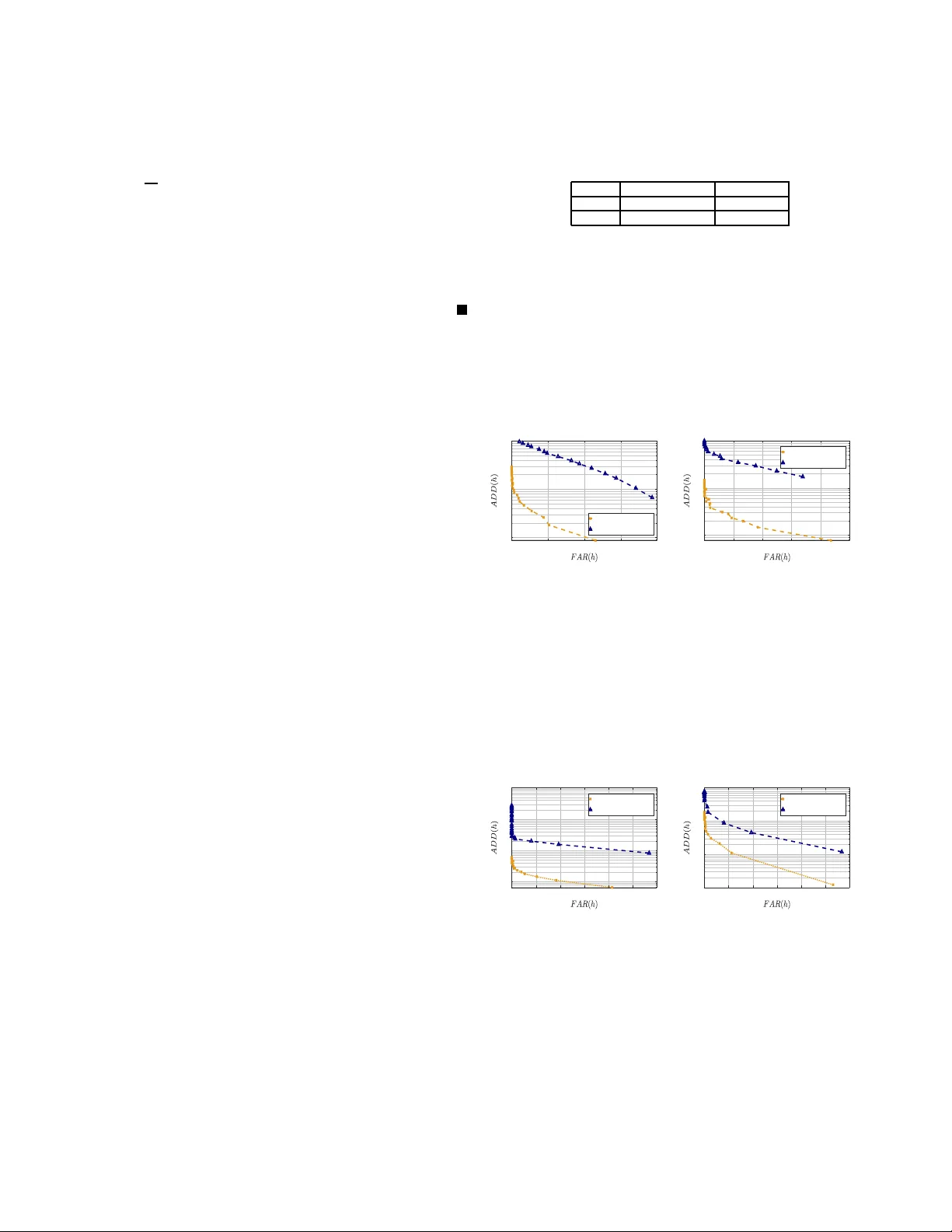
OT - D E T E C T : Optimal tr anspor t-driv en attac k detection in cyber-ph ysical systems Souvik Das and Siddhar tha Ganguly Abstract — This article presents an optimal-transpor t (O T)-driven, distributiona lly robust a ttack detection algo- rithm, OT - D E T E C T , for cyber–physi c al systems (CPS ) mod- eled as partial ly obse rved linear stochastic sy stems. The underlying de tection problem is formulated as a minmax optimization problem us i ng 1 -W asserstein ambig uity sets construc ted from o bserv er residuals unde r both t he nom- inal (attack-free) a nd a ttacked reg imes. We show that the minmax detecti on problem can be re duced to a finite- dimension al l inear program f or computin g t h e worst-case distribution (WCD). Off-suppor t residu als are handled via a ke rnel-smoothe d sc ore functio n that drives a CUSUM procedure for seque ntial detection. We also e stablish a non-asy mptotic tail b ound o n the false -positive error of the CUSUM s tatistic un der the nominal (atta ck-f ree) c ondition, under mild assumpti ons. Numerical illu strations are pro- vided to evaluate the robustne ss propertie s of O T - D E T E C T . Index T e rms — Cyber-physica l sys tems, optimal tra n s- port, attack detection I . I N T R O D U C T I O N , M OT I VA T I O N , A N D B AC K G R O U N D Cyber-physical systems (CPS) — ran ging fr om in d ustrial control loops and autono m ous vehicles to b iomedical and energy infrastructur es — m ust operate reliab ly amid uncertain - ties like sensor noise, model mismatches, and, increasingly , intelligent adversaries that tamp er with senso r o r actuator signals. In conte m porary research o n the secur ity and pr ivac y of CPSs, particularly studies fo cused o n attack d etection, the process noise is typ ic a lly assumed to be Gaussian and fu lly known to bo th the controller (or designer) and the adversary . While this assum ption is useful fo r d istinguishing inherent model unce rtainties from adversarial disturbance s, it is of ten unnatur al. More over, adversaries in CPSs are often mod eled as resource- lim ited agents governed by a predefined attack mo del. Howe ver , a strategic adversary may defy such assumption s by actively co llu ding, remaining stealthy and covert to gather informa tio n, and explo itin g th e lear ned system knowledge to mount sophisticated and large-scale attacks. A related study in this context h as been done in [1], wher e a ne w idea based o n separation of state trajecto r y was introdu ced. Residual-based d etectors for attacks typically d epend on distributional assumption s and fixed- model likelihood ratios; while effective when nom in al and attack distributions are S. Das is with the Division of Signals and S ystems , Uppsala Uni- v ersity , Sweden. S. Ganguly is with the Daniel Guggenhei m School of Aerospace Engi neering, Georgia Institute of T echnology , USA. Emails: {dsouv .ct@gmail.com, sganguly41@gatech.edu}. precisely known, they falter under distrib utional u ncertainty or whe n adversaries intentionally g uide observations into am- biguou s re gimes. This undersco res the need fo r distributionally r obust testing rules that ( i) impo se minimal assumption s o n data-gen e rating processes and (ii) explicitly incor porate worst- case d istrib utional shifts relati ve to the observed d ata. Related works: A few works employ distributionally robust optimization for attack detection. Sp ecifically , [2] uses OT - driven W asserstein a m biguity sets for the unknown disturbance distribution and op timizes a reachability-b ased performance metric, to d e sig n a par ity -space detector . [3] in stead work with moment- based ambiguity sets an d then compu te ellipsoidal attack-reach able sets ; this gives worst-case false alarm rate control under second-m o ment information , but the d e te c tor it- self remain s a co n ventional q uadratic test, with no W asserstein geometry between benign/attack distributions and no explicit min–max optimal test or sequential statistic. For sensor attacks, [4] leverages W asserstein metrics, b ut as a d istance between a ben chmark residual distribution and a sliding-window em- pirical distribution, recom puted online via a linear pr ogram; sequential detection and false po siti ve bound s were no t studied . In con trast, our ma in contributions are: ◦ An O T - driven detection: For a stochastic linear tim e- in variant ( L TI) p lant equipp ed with a steady-state observer, we devise a new d ata-driven residual-based detector, lev er- aging tools fr om O T , DR O, and hy pothesis testing . W e formu late the detection problem as a min-max hypoth esis test b etween two amb ig uity sets of prob ability measures. Drawing results from [5] an d Kantorovich–Rub instein du- ality [6], we show th at the comp utation of worst-case distribution (WCD) re d uces to a finite line a r pr ogram ( LP) ; informa lly Inf ormal Theorem A: Let Q 1 , Q 2 be the em p irical measures of residuals on the finite set b Ω : = { s ℓ } n ℓ =1 (training win d ow), an d let P k : =  P   W 1 ( P, Q k ) 6 ε k  for k ∈ { 1 , 2 } . The min max testing risk equals ε ⋆ = 1 − V ⋆ , where V ⋆ is the optimum of a finite linea r pr ogram . See Th eorem 1 f or fur ther informa tio n. ◦ Ker nel smoothing and sequential CUSUM-based test: While the LP exactly s olves the on-supp o rt d etection pr ob- lem, real-time deployment mu st e valuate the test o n new r esiduals z which may n ot be in the training set. T o extend beyond the on-support training d ata, we present a kernel- smoothing con struction that maps the discrete WCDs to continuo us densities and uses the log-den sity ratio as a continuo us scor e, attractive for sequen tial operatio n. ◦ Non-asymptot ic bounds o n the false-positive error: Be- yond algor ithmic trac ta b ility , we pr ovide non- asymptotic guarantees on the tail boun d for the f alse positiv e error; informa lly Inf ormal Theorem B: Run th e CUSUM recursion S 0 = 0 , S t = max { 0 , S t − 1 + X t } . Unde r mild condition s on the increm ents, for any threshold h > 0 : P 1 ( S t > h ) 6 2 exp  − h 2 / 8 t X i =1 σ 2 i  , where σ i > 0 known. See Th eorem 2 f or fur ther details. The key features o f this work are as follows: (a) Our detection scheme does not requir e full distributional knowledge of the process noise, only that it lies in an ambiguity set specified by 1-W asserstein distance, ensuring distributional robustness. (b) Our detectio n scheme is adversary-agnostic , with no assumptions o n the attack model nor on the policy employed by the adversary . (c) W e assume the ad versary has access to system par ameters, n ominal c ontrol policies, and sensor measuremen ts. They can learn stead y-state beh avior, ada pt to system cha nges, collude, and lau nch attacks acco rdingly to disrupt attac k-free perf ormance. I I . P R E L I M I N A R I E S A N D P R O B L E M D E S C R I P T I O N Let d ∈ N ∗ be a natu ral num ber and p ∈ [1 , + ∞ [ ; let Ω ⊂ R d with the m etric d Ω : Ω × Ω − → [0 , + ∞ [ . By P (Ω) we deno te t he set (rich enough) of Borel probability measures o n Ω . W e assume that the pro bability measures under co n sideration are absolu tely continuo us with respect to the Lebesgu e mea sure o n suitable domain s, and we id entify each such measur e with its d ensity . Thus, if µ, ν ∈ P (Ω) , we write d µ ( x ) = µ ( x ) d x and d ν ( y ) = ν ( y ) d y . Define the set of no nnegativ e and integrable tr ansport pla ns by Π( µ, ν ) : =  π   R Ω π ( x, y ) d y = µ ( x ) , R Ω π ( x, y ) d x = ν ( y )  6 = ∅ . The p -W asserstein distance is defined by [6 , Ch. 6, Def. 6.1 ] W p ( µ, ν ) : =  inf π ∈ Π( µ,ν ) Z Ω 2 d Ω ( x, y ) p π ( x, y ) d x d y  1 /p , (1) The variational p roblem o n the left-hand side of (1), for p = 1 , is the st andard Kantorovich-Rubinstein O T pro blem [6]. Th e W asserstein distance quantifies the min imal “cost” measured via d ( · , · ) (which is ty pically th e stand a rd Euclid e an distance) of transpo rting mass in Ω to transf o rm µ in to ν . The cost (1) n a turally arises in DR O; indeed, in DR O the goal is to hedg e against u ncertainty by optimizing the worst-case expected loss ov er an ambiguity set of distributions c entered around a nominal one. O T costs, such as (1), naturally emerge as a prin cipled choice for defining this ambig uity set because they quan tify distributional discrepanc ies while re sp ecting the underly ing geometry and metric stru cture o f the data space [7], [8]. This enab le s mo d eling r ealistic perturba tions, yield ing interpretab le a nd tractable robust mod els, ideal for many applications in machine and control theory [9] –[13]. In the sequel, our context will be discr e te measur es an d thus simpler . W e den ote th e standard p robability simplex by Σ d : = { ζ ∈ R d  0 | P d i =1 ζ i = 1 } . Fix natural n umbers n, m > 1 , an d let a : = ( a 1 , . . . , a m ) ⊤ ∈ Σ m and b : = ( b 1 , . . . , b n ) ⊤ ∈ Σ n . On Ω define the discrete m easures µ : = P m i =1 a i δ x i and ν : = P n j =1 b j δ y j ; where x i , y j ∈ Ω are the supp ort points. Define the set of coup lings (which is a conve x p olytope) by Π( a , b ) : =  P ∈ R m × n +     n X j =1 P ij = a i , m X i =1 P ij = b j  . Consequently , ( 1) takes the fo rm (for p = 1 ) W 1 ( µ, ν ) : = inf P ∈ Π( a , b ) m X i =1 n X j =1 P ij k x i − y j k . (2) In the detection pr oblem, we will constru ct o ur ambig uity sets e m ploying the W 1 metric (2), which is often called the Kantor ovic h-Rub instein distance [6, Chapter 6 ]. A. Stochastic linear systems Let d x , d u , d w and d y be natural nu mbers. Con sider a time- in variant d iscrete-time contro l system x t +1 = Ax t + B u t + E w t , y t = C x t + F w t , (3) with x 0 : = x g i ven and t ∈ N , along with the following data: x t ∈ R d x , u t ∈ R d u , w t ∈ R d w , and y t ∈ R d y are the vectors represen tin g the states, contr ol inputs, un certainties, and the o utput at time t , with A ∈ R d x × d x , B ∈ R d x × d u , E ∈ R d x × d w , C ∈ R d y × d x and F ∈ R d y × d w . The controller computes the state estimate, which is a func tion of the observa- tion ( y t ) t ∈ N , to estimate and mo nitor the system, and employ control actions that are a function of th e state estimate. Let L ∈ R d x × d y be a steady-state gain, we consider the estimator: b x t +1 = A b x t + B u t + L ( y t − C b x t ) , r t : = y t − C b x t , (4) with b x 0 : = b x . Moreover , L is p icked such that th e spectrum of ( A − LC ) lies in the unit circle. Assumption 1: Th e 3 -tu ple ( A, B , C ) is b oth stab ilizab le and d etectable. W e mo del the influence of the adversary by th e s tochastic process e w that enters the system throug h th e o utput channel: for t ∈ N , we have the recu rsion x a t +1 = Ax a t + B u a t + E w t , y a t = C x a t + F w t + e w t . (5) where x a 0 : = x is given. Here, the contro ller’ s ac tio n u a t at each time is based o n th e available corrup ted output ( y a t ) t ∈ N . The co r respondin g state estimator is g i ven by the recursion b x a t +1 = A b x a t + B u a t + L ( y a t − C b x a t ) with b x a 0 : = b x a , r a t : = y a t − C b x a t , (6) where L ∈ R d x × d y is the steady - state gain, chosen similarly . Under the above setting, we seek to infer whether the system’ s uncertainties are inherent, represen ted by w , o r they have bee n influenced by an external unwanted ad versarial disturbanc e denoted by e w . Inf ormally , we pose this problem as a composite hypothe sis testing pr o b lem : gi ven a samp le ω o f the residual obtained fr om (4) an d (6), we set: (H0): ω ∼ P 1 ∈ P 1 and (H 1 ): ω ∼ P 2 ∈ P 2 , where P 1 and P 2 are the sets of pro bability measures defined over a set Ω ; see (8) for a definition. I I I . T H E O P T I M A L D E T E C T O R W e are ready to formulate th e hypo th esis testing pro b lem. Recall that the underlyin g d istributions o f w and e w are not av ailable. Howe ver , we hav e acc e ss to n 1 ∈ N ∗ and n 2 ∈ N ∗ number of residual samp les as the training data . Precisely , let Ω : = R d y and we consider the data streams: Ω 1 : =  b r i ∈ Ω  n 1 i =1 and Ω 2 : =  b r a j ∈ Ω  n 2 j =1 , and let b Ω : = Ω 1 ⊔ Ω 2 = { s ℓ } n ℓ =1 with n : = n 1 + n 2 . Let α ∈ Σ n 1 , β ∈ Σ n 2 ; we construct the empirical measures Q 1 : = n 1 X i =1 α i δ b r i and Q 2 : = n 2 X j =1 β j δ b r a j , (7) with α i = 1 n 1 and β j = 1 n 2 for all ( i, j ) ∈ { 1 , . . . , n 1 } × { 1 , . . . , n 2 } . W e also define the index sets I 1 : = { 1 , . . . , n 1 } and I 2 : = { n 1 + 1 , . . . , n } with b I : = { 1 , . . . , n } . In shorthand notation, for ℓ = 1 , . . . , n 1 we hav e s ℓ = b r ℓ and for ℓ = n 1 + 1 , . . . , n , we have s ℓ = b r a ℓ − n 1 . W e expand (7) in the unified index ℓ , and to wards this end , we define f o r ℓ ∈ { 1 , . . . , n } , the empirical m easures ( Q 1 ) ℓ : = α i for ℓ ∈ I 1 , and ( Q 2 ) ℓ : = β ℓ − n 1 for ℓ ∈ I 2 under the nominal and attacked case, respectively . Note th at f or k = 1 , 2 , ( Q k ) ℓ = 0 for ℓ ∈ b I \ I k because th eir corresp o nding supports are disjoint. W e cho ose the gro und cost d Ω defined in (1) to b e the Euclidean distance ( z , z ′ ) 7→ d Ω ( z , z ′ ) : = k z − z ′ k 2 . And for some ε 1 , ε 2 > 0 , we con sider two ambiguity sets centred around e m pirical distributions Q k for k = 1 , 2 , given by P k : =  P k ∈ P (Ω)   W 1 ( P k , Q k ) 6 ε k  for k ∈ { 1 , 2 } , (8) where W 1 ( · , · ) is the 1 - W asserstein distance defined in (2). The minmax test: W e fo rmulate a min max test ba sed on the ideas advanced in [5], [14]. Recall that, given hypotheses (H0) and (H1), a rando mized test is any Borel measurab le map T : Ω − → [0 , 1 ] , which for any observation s ℓ ∈ Ω , accepts th e hyp othesis (H0) w ith probability equ al to T ( s ℓ ) and (H1) with pr obability equal to 1 − T ( s ℓ ) . 1 For a pair ( P 1 , P 2 ) ∈ P 1 (Ω) × P 2 (Ω) , define risk fun ction R  T ; P 1 , P 2  : = E 1 [1 − T ( s ℓ )] + E 2 [ T ( s ℓ )] . (9) Then, the robust testing pr oblem is inf T sup P 1 ∈P 1 ,P 2 ∈P 2 R ( T ; P 1 , P 2 ) . (10) Note that th e risk f unction (9) acco unts f or the tra de-off between likelihood o f incurring err ors by the test T ( · ) under P 1 and P 2 , r espectiv ely . 1 Throughout, we abuse nota tion by referr ing to random vecto rs and their realiz ations using the same symbols. A. LP f ormulation In [5], [ 14] it was shown that in the setting o f simple hypothe sis testing , the optimal test takes a similar form as the likelihood r atio test. More precisely: Lemma 1: For any fixed ( P 1 , P 2 ) ∈ P 1 × P 2 , consider the inner minim iz a tio n problem R( P 1 , P 2 ) : = inf T :Ω − → [0 , 1] R ( T ; P 1 , P 2 ) (11) correspo n ding to the minmax pro blem (1 0). Then the Neyman- Pearson-like rando mized rule T ⋆ ( s ℓ ) : =      1 if d P 2 d( P 1 + P 2 ) ( s ℓ ) > 1 2 0 if d P 1 d( P 1 + P 2 ) ( s ℓ ) < 1 2 p ∈ [0 , 1 ] otherwise (12) is optima l f o r the (11) with the risk R( P 1 , P 2 ) = 1 − TV ( P 1 , P 2 ) . ♦ T o find the worst-case distributions (WCD), we need to look at the inner suprem um problem in (10), i.e., sup P 1 ∈P 1 ,P 2 ∈P 2 1 − TV ( P 1 , P 2 ) . (13) The variational problem (13) is infinite-dimen sional and is n ot computatio nally viable in gene r al. But due to the nature of the W 1 -ambigu ity set and the d iscreteness of the empirical measures, we can o ptimally solve (13) via a finite- dimensional tractable conve x program, which is the fo cus of th e next result. Note that (13), if it admits a solution, ensures that the overlapping distributions P 1 and P 2 correspo n ding to th e nominal condition and under-attack con d ition, h a ve to be clo se in th e total variation sense ( T V -sense), thereby co nstraining the adversarial policy . In oth er words, the adversary canno t act freely to in flict ser ious damage a n d d egrade the perfor mance to a large extent, else risk detection. Theorem 1: Recall th at the no tations established in §II. Correspon d ing to th e ground cost d Ω ( · , · ) we define the pairwise cost matrix D ∈ R n × n + with D ℓm : = d Ω ( s ℓ , s m ) . Consider th e robust testing problem ε ⋆ : = inf T sup P 1 ∈P 1 , P 2 ∈P 2 E 1 [1 − T ( s ℓ )] + E 2 [ T ( s ℓ )] , (14) where th e ambiguity sets are defined in (8). (a) Then ε ⋆ = 1 − V ⋆ . Where V ⋆ is the op timal value of the following finite linear pr ogr am with decision variables b p : = ( p 1 , p 2 , Γ 1 , Γ 2 , t ) : p 1 , p 2 ∈ R n + with P ℓ p k,ℓ = 1 , Γ 1 , Γ 2 ∈ R n × n + (optimal tr ansport couplin gs from empirical m easures Q k to p k ), and t ∈ R n + : max b p n X ℓ =1 t ℓ s . t .                P n ℓ =1 P n m =1 Γ 1 ,ℓm D ℓm 6 ε 1 , P n ℓ =1 P n m =1 Γ 2 ,ℓm D ℓm 6 ε 2 , P n m =1 Γ k,ℓm = ( Q k ) ℓ , P n ℓ =1 Γ k,ℓm = p k,m , 0 6 t ℓ 6 p 1 ,ℓ , 0 6 t ℓ 6 p 2 ,ℓ , p k,ℓ > 0 P n ℓ =1 p k,ℓ = 1 , Γ k,ℓm > 0 for all k ∈ { 1 , 2 } . (15) (b) The LP (15) is well- posed and admits a so lu tion. ♦ Proof: For any fixed ( P 1 , P 2 ) , via Lemma 1 we have inf T E 1 [1 − T ( s ℓ )] + E 2 [ T ( s ℓ )] = 1 − T V ( P 1 , P 2 ) , which imp lies ε ⋆ = 1 − inf P 1 ∈P 1 ,P 2 ∈P 2 TV ( P 1 , P 2 ) . Because Q k is discrete on b Ω , the balls P k admits the standard O T -co upling repr esentation. Indeed, since p k = P n m =1 p k,m δ s m on b Ω , u sing the duality argumen ts a nd pro p- erties of W 1 ( · , · ) via [5, Lemma 6 an d Lemma 8], th ere exists a coup ling m atrix Γ k ∈ R n × n + between Q k and p k with row s ums ( Q k ) ℓ , column sums p k,m , and cost bound ed by ε k , i.e., P n m =1 Γ k,ℓm = ( Q k ) ℓ , P n ℓ =1 Γ k,ℓm = p k,m and P ℓ,m Γ k,ℓm D ℓm 6 ε k , with D ℓm : = d Ω ( s ℓ , s m ) . Note that the finite-redu ction at at atoms s ℓ again follows fro m the Kantorovich- Rubinstein-type Duality [5, Lemma 6 ]. Since both the d istributions are discrete on the same finite support b Ω , we ha ve: T V ( p 1 , p 2 ) = 1 − P n ℓ =1 min { p 1 ,ℓ , p 2 ,ℓ } . Introd u cing v ariables t : = ( t 1 , . . . , t n ) ∈ R n + with 0 6 t ℓ 6 p 1 ,ℓ , 0 6 t ℓ 6 p 2 ,ℓ with ℓ = 1 , . . . , n , we see th a t max t ∈ R n +  n X ℓ =1 t ℓ     0 6 t ℓ 6 p 1 ,ℓ , 0 6 t ℓ 6 p 2 ,ℓ  (16) is eq ual to P n ℓ =1 min { p 1 ,ℓ , p 2 ,ℓ } . T h e precedin g arguments along with (16) yields exactly th e finite LP in the proposition , hence ε ⋆ = 1 − V ⋆ . W e show the well-posedness and existence of solu- tions to (15). Feasibility is immediate: choose p k = Q k , Γ k,ℓm : = ( Q k ) ℓ 1 m = ℓ , and t ℓ : = 0 . 2 Then by construction P m Γ k,ℓm = ( Q k ) ℓ and P ℓ Γ k,ℓm = p k,m = ( Q k ) m , also P ℓ,m Γ k,ℓm D ℓm = P ℓ ( Q k ) ℓ D ℓℓ = 0 6 θ k since D ℓℓ = d Ω ( s ℓ , s ℓ ) = 0 ; a n d t ℓ = 0 6 p 1 ,ℓ , p 2 ,ℓ . Hence, the feasible set is non empty . The feasible set is defin e d by bo unded line a r equalities and inequalities in a finite-dimen sional Eu clidean space and thu s is compa c t, an d ( p, Γ , t ) 7→ P ℓ t ℓ is contin - uous. Ex istence of a solution follo ws immed iately from the W eierstrass theorem. On sample te st: Note that, any o ptimizer of (15) pro duces the WCD, P ⋆ k : = P n ℓ =1 p ⋆ k,ℓ δ s ℓ for k ∈ { 1 , 2 } . Then the on- support op timal test values are T ⋆ ( s ℓ ) =      1 , if p ⋆ 2 ,ℓ > p ⋆ 1 ,ℓ , 0 , if p ⋆ 2 ,ℓ < p ⋆ 1 ,ℓ , ∈ [0 , 1] , if p ⋆ 2 ,ℓ = p ⋆ 1 ,ℓ ( ties ) . (17) In case of a tie, T ∗ ( s ℓ ) choose either 1 or 0 w .p. 1 / 2 . W ith this T ∗ , we h a ve the worst-case risk ε ⋆ = P n l =1 p ⋆ 1 ,ℓ (1 − T ⋆ ( s ℓ )) + p ⋆ 2 ,ℓ T ⋆ ( s ℓ ) = 1 − P n ℓ =1 t ⋆ ℓ . B . K ernel smoothing The LP (15) identifies Th e WCD’ s P ⋆ k for k = 1 , 2 , on the training atom s b Ω and the test T ⋆ ( s ℓ ) on th ose atoms. While this fully resolves the on-suppo rt problem and also enab les sequential use when the test p oint coin c id es with an atom , in deployment, however , incom in g residuals z ∈ Ω will rarely lie exactly on b Ω . Thus, to d efine th e d e te c tor f or every z , o n e must extend T ⋆ off-support. T o this end, we adopt a kerne l smoothing tech nique, which is often p referable in practice because o f its compatibility with sequ e n tial testing. 2 Here 1 A ( · ) is the s tandard indicator function for a gi ven set A ⊂ R . K er nel smoothing and a CUSUM te st: Choose a kernel K : R d − → [0 , + ∞ [ with R R d K ( t ) d t = 1 and b a ndwidth σ > 0 . Set ξ 7→ K σ ( ξ ) : = 1 σ d K  ξ σ  . Then , for k = 1 , 2 , define Ω ∋ z 7→ f k ( z ) : = n X ℓ =1 p ⋆ k,ℓ K σ ( z − s ℓ ) . (18) Define the scor e function by z 7→ s K ( z ) : = log f 2 ( z ) f 1 ( z ) = lo g P n ℓ =1 p ⋆ 2 ,ℓ K σ ( z − s ℓ ) P n ℓ =1 p ⋆ 1 ,ℓ K σ ( z − s ℓ ) . (19) While there are many choices f or the kernel f unction, we will pick the Gaussian kernel ξ 7→ K σ ( ξ ) : =  2 π σ 2 ) − d/ 2 exp  − k ξ k 2 2 / 2 σ 2  because of its nice properties as specified in Remark 1 ahead. Remark 1 (F eatur es of the Gaussian kernel smooth ing): Note th a t ξ 7→ K σ ( ξ ) > 0 implies tha t z 7→ f k ( z ) > 0 , this makes the score fun ction (19) well-defin ed and finite ev erywhere . Gau ssian smooth ing makes f k ( · ) an d s K ( · ) smooth and from a n umerical point of vie w each lo g f k ( z ) is a log- sum-exp of q uadratic terms which is stable to compute and e a sy to trun c ate to K nearest atoms for speed. Moreover s K ( s ℓ ) − → log p ⋆ 2 ,ℓ p ⋆ 1 ,ℓ as σ ↓ 0 , which m atches the Neyman-Pearson -like test on the atoms. ♦ Define the incr ements sequence ( X t ) t ∈ N : = ( s K ( z t )) t ∈ N . W e consider the CUSUM recursion [ 15] S 0 : = 0 , S t : = ma x { 0 , S t − 1 + X t } , for t > 1 , (20) and we test S t for every time t , ag ainst some appro priately chosen thresh o ld h : ( S t > h Reject (H0) in f av or of ( H1), S t < h Reject (H1) in f av or of ( H0) . The method to cho ose the threshold is detailed in §V. W e now outline all these key steps as the following Algor ith m. OT - D E T E C T : OT -based detection algorithm for CPS. Initialize : S 0 = 0 Data : Stream of offline n o minal data b r , kernel fun ction K σ , h > 0 1 Construct th e training data b Ω 2 Solve (15) to compute the LFDs ( P ⋆ 1 , P ⋆ 2 ) on b Ω 3 Extend ( P ⋆ 1 , P ⋆ 2 ) by kernel smoothing to obtain (19) 4 for t = 1 , 2 , . . . , do 5 Compute the sequence ( S t ) t ∈ N defined in (20) 6 Raise an alarm if S t > h , else continu e Step 5 7 end I V . T H E O R E T I C A L G UA R A N T E E S W e establish n on-asymp totic guara n tees on the false positive error under (H0 ) with P 1 , incurr ed b y the algorithm , which states that un der the attack-f ree r egime the e vent { S t > h } admits a low pr o bability . During deploymen t, this error serves as a practical guid e to select an appro priate threshold ; see § V for a discussion on it is utilised to select a threshold . Theorem 2: Le t (Ω , F ) be a measurab le space and F t : = σ ( X 1 , . . . , X t ) th e natu ral filtration. Let X t ∈ R be an F t - adapted sequence with E 1 [ | X t | ] < + ∞ . Recall the CUSUM iteration in (20). For ea ch i , define th e co nditional drift and the centered incr ements µ i : = E 1 [ X i | F i − 1 ] and ξ i : = X i − µ i , and assume that under P 1 , the distribution under (H0), the condition al drift is n on-po siti ve: µ i = E 1 [ X i | F i − 1 ] 6 0 a.s. for i = 1 , . . . , t. (A1) and tha t there exists known constan ts σ 1 , . . . , σ t > 0 such that for every λ ∈ R and ev ery i = 1 , . . . , t : E 1 [exp  λξ i  | F i − 1 ] 6 exp  λ 2 σ 2 i / 2  a.s. , (A2) where E 1 is a exp e ctation under (H0 ). Define V t : = P t i =1 σ 2 i . Then f or every h > 0 , we ha ve the bo und P 1  S t > h  6 2 exp  − h 2 / 8 V t  . (21) Remark 2: Un d er the n o minal law P 1 , Assump tion A1 imposes a n on-po sitive drift cond ition on the scor e increments: condition ally on the past, X i should not, on av erage, drive the CUSUM statis tic u p ward. T h is is natu ral, since in th e no- attack regime, the detector should ha ve n o tendency to cross an appr opriately c hosen threshold. Assumption A2 is a co n- ditional s ub-Ga u ssian requireme n t on th e cente r ed increm ent ξ i = X i − µ i , and co ntrols the rando m fluctuations o f the score around its predictable drift µ i . Th e CUSUM sequenc e ( S t ) t ∈ N is com patible with standard pr eprocessing techniqu es such as satu ration or clippin g, which render the scor e function uniformly bou n ded and thus enf orce As sumption A2 b y con- struction [16]. Consequ e ntly , Assumptions A1 and A2 r emain sufficiently general to accommo d ate a wide class of score function s ( 19). ♦ Proof: [ Proof of Theo rem 2] Define A t : = P t i =1 X i with A 0 : = 0 . Then, th e CUSUM identity can b e written as S t = A t − min 0 6 k 6 t A k = max 0 6 k 6 t  A t − A k  . (22) T o see this, define B t : = A t − min 0 6 k 6 t A k with B 0 = 0 . Since min 0 6 k 6 t A k = min { min 0 6 k 6 t − 1 A k , A t } , we get B t = ma x  A t − min 0 6 k 6 t − 1 A k , 0  = ma x  B t − 1 + X t , 0  , which is exactly the CUSUM recur sio n with S 0 = 0 . Hence B t = S t . Let us now de fin e the F t − 1 -measurab le one step ahead con ditional mean of X t and the inn ov ation or centered incremen t, respective, b y µ i : = E 1 [ X i | F i − 1 ] and ξ i : = X i − µ i . Note that, since E 1 [ X i ] < + ∞ we have E 1 [ µ i ] < + ∞ ; mo reover , ξ i has zero cond itio nal me an, i.e., E 1 [ ξ i | F i − 1 ] = E 1 [ X i − µ i | F i − 1 ] . Now co nsider the cumulative innovation sequen ce M t : = P t i =1 ξ i and the predictable p r ocess D t : = P t i =1 µ i . Note that M t is a fin ite sum of integrable F i -measurab le terms, so it is F t -measurab le and in tegrab le. Moreover , we ha ve E 1 [ M t | F t − 1 ] = E 1 h M t − 1 +  X t − µ t     F t − 1 i = M t − 1 + E 1 [ X t | F t − 1 ] − µ t = M t − 1 . Thus, ( M t , F t ) is a Martingale. W e show that  D t  t > 1 is a pr edictable process [1 7, Section 1 .4]: for t > 1 , we h a ve D t = P t i =1 µ i , and eac h µ i is F i − 1 -measurab le. Becau se F i − 1 ⊆ F t − 1 when i 6 t , th e su m is F t − 1 -measurab le. Hence ( D t ) t > 0 is pr edictable, i.e., D t is F t − 1 -measurab le for t > 1 . Moreover it is integrable: indeed, we have E 1 [ µ i | 6 E 1  | X i |  < + ∞ an d conseque n tly , f or any finite hor iz o n t , E 1  | D t |  6 P t i =1 E 1  | µ i |  6 P t i =1 E 1  | X i |  < + ∞ . Finally , by definition D 0 = 0 . Th u s, all the con ditions fo r the Doob’ s decomp osition theorem [17 , Theorem 4.10 ] are met and we hav e A t = M t + D t . Also, d ue to Assum ption (A1), µ i 6 0 a.s. f or all i an d D t − D k = P t i = k +1 µ i 6 0 a.s., and th u s, D t is non- increasing. Now , u sin g (22) and A t − A k = ( M t − M k ) + ( D t − D k ) along with the preceding arguments, we see that S t = max 0 6 k 6 t ( A t − A k ) 6 max 0 6 k 6 t  M t − M k  a.s. (23) Using the fact that for any r eal n umbers x, y a nd h > 0 , x − y > h implies x > h/ 2 or − y > h/ 2 we see tha t { max 0 6 k 6 t ( M t − M k ) > h } is subset of the union n max 1 6 s 6 t M s > h 2 o ∪ n max 0 6 s 6 t ( − M s ) > h 2 o . (24) Combining ( 23)–(24), { S t > h } ⊆ n max 1 6 s 6 t M s > h 2 o ∪ n max 0 6 s 6 t ( − M s ) > h 2 o . (2 5 ) W e now show tha t, for a > 0 the c oncentration bou nd holds: P 1  max 1 6 s 6 t M s > a  6 e xp  − a 2 / 2 V t  . (26) Then we will apply the same bo und to − M s . T o this end , fix λ > 0 an d defin e the process Z s : = exp  λM s − λ 2 2 V s  , for s = 0 , 1 , . . . , t, with M 0 = 0 , V 0 = 0 , hence Z 0 = 1 . W e show that ( Z s , F s ) is a nonnegative sup ermartinga le. Indeed, writing the martingale increment: M s = M s − 1 + ξ s and V s = V s − 1 + σ 2 s , we see that Z s = exp  λ ( M s − 1 + ξ s ) − λ 2 2 ( V s − 1 + σ 2 s )  = Z s − 1 · exp  λξ s − λ 2 2 σ 2 s  . T aking co nditional expectation w .r .t F s − 1 and re calling that Z s − 1 is F s − 1 -measurab le, we get E 1 [ Z s | F s − 1 ] = Z s − 1 E 1 h exp  λξ s − λ 2 2 σ 2 s     F s − 1 i = Z s − 1 e − λ 2 2 σ 2 s E 1 h e λξ s | F s − 1 i 6 Z s − 1 , where in the last step we employed (A2). Thus ( Z s , F s ) is a nonnegative supermartin gale. W e also note th at using mon otonicity of the expon ential and using the fact that V s 6 V t for s 6 t , the event { ∃ s 6 t | M s > a } im plies {∃ s 6 t | Z s > c } where c : = exp  λa − λ 2 2 V t  . T h en we h a ve the inclusion n max 1 6 s 6 t M s > a o ⊆ n max 1 6 s 6 t Z s > c o . (27 ) Define the hitting tim e τ : = inf { 1 6 s 6 t | Z s > c } , with the conv ention τ = + ∞ if no su ch s exists. Then { max 1 6 s 6 t Z s > c } = { τ 6 t } . Define the bounded stopping time τ ′ : = min { τ , t } so that τ ′ 6 t always. Since Z s is a nonn egati ve superma rtingale and τ ′ is bou nded, o n e h as E 1 [ Z τ ′ ] 6 E 1 [ Z 0 ] = 1 . Moreover, o n th e event { τ 6 t } we have τ ′ = τ and Z τ ′ = Z τ > c . Hen ce Z τ ′ > c 1 { τ 6 t } . T a king expectation a nd recalling the fact tha t E 1 [ Z τ ′ ] 6 1 , we obtain P 1  max 1 6 s 6 t Z s > c  6 (1 /c ) . (28) From (2 7) and ( 28) we ha ve P 1  max 1 6 s 6 t M s > a  6 P 1  max 1 6 s 6 t Z s > c  6 (1 /c ) . (29) Optimizing the right-hand side of (29) with respe c t to λ > 0 giv es ¯ λ = a V t and th is yields the required bound (2 6). The identical argument ap p lied to − M s (noting that (A2) holds fo r all λ ∈ R , hence also for − ξ i ) g i ves P 1  max 0 6 s 6 t ( − M s ) > a  6 exp( − a 2 / 2 V t ) . (30) Finally , ( 26)–(30) (with a = h / 2 ) tog ether with (25) gi ves us P 1 ( S t > h ) 6 ex p  − h 2 / 8 V t  . Th e proo f is comp le te. V . N U M E R I C A L VA L I DA T I O N A N D D I S C U S S I O N W e com pare the perfor mance of o ur d etector with that of the o ptimal CUSUM detector [1 5] in Gaussian settings an d provide positive r esults in certain no n-Gaussian regimes. System description: W e con sid ered a be nchmark linearized fourth - order quadr uple-tank proc ess [18 , Eq. 1 ] for our exper- iments. Th e system param eters are given by A =    0 . 968 0 0 . 082 0 0 0 . 978 0 0 . 064 0 0 0 . 917 0 0 0 0 0 . 935    , B =    0 . 164 0 . 004 0 . 002 0 . 124 0 0 . 092 0 . 06 0    , with C = I 4 (the (4 × 4) ide ntity matrix). Perf ormance metrics: L et T at denotes the unknown but deterministic time when the attack was initiated . Let T d be the time when the algorith m de tects the a ttack, defined by T d : = inf  t ∈ N   S t > h  for a fixed thresh old h . For a giv en toler ance η ∈ ]0 , 1] , the threshold h is estimated such that P 1 ( S t > h ) = η , where η > 0 is th e pre-defined threshold on the incurred false positive error u nder (H0). W e considered the follo wing standard metr ics to assess the perfo rmance: ◦ A vera ge detectio n delay (ADD) : For a fixed th reshold h , ADD is defined by ADD( h ) : = E 2  T d − T at   T d > T at  , where th e expectatio n is d efined with respect to the probab ility m e a sure und er (H1), an d h is the thr eshold. ◦ F alse alarm r ate (F AR): Fix h , and compu te F AR as F AR( h ) : = P 2  T d < T at  , whe re the prob ability measure is defin e d with respect to (H1) . In the experim ents, we examined ADD with respect to F AR for different values of h , which reveals how quick ly the attack is detected fo r a given toler ance of F AR( h ) . Mon te-Carlo simulations were co nducted to comp u te ADD( · ) and F AR( · ) . Attack mo del: For all e xperimen ts, we considered the decep- tion attack [15] described b y the process v t = A a v t − 1 + b v t , where A a ∈ R d y × d y . The seq u ence ( b v t ) t ∈ N refers to the uncertainties associated with the adversary . W e con sidered the f ollowing two cases: (a) ( b v t ) t ∈ N is a seq uence of d y - dimensiona l Gaussian random vector with covariance Σ a ; (b) ( b v t ) t ∈ N was gen e r ated from Gaussian distribution N (0 , Σ a ) corrup ted b y Exp( λ ) , where λ > 0 is a pa r ameter . It is assumed that durin g the attack , the adversary , with approp riately chosen ( A a , Σ a ) , may co mp letely r eplace the true ou tput signal y with the corr upt data g e nerated by the process v . W e fixed th e attack starting time to b e 250 second s (considere d to be determ inistic b ut unk nown to the defender) . Parameters: Th e bandwid th σ > 0 of the Gaussian kernel was picked to be 0 . 5 . For repro ducibility , we fixed the seed to be 2 . T able I summ a r izes the ch oice of the parameters. Results: First, we considered the setting where we assumed ( ε 1 , ε 2 ) ( n 1 , n 2 ) Fig. 1 (0 . 001 , 0 . 001) (150 , 150) Fig. 2 (0 . 001 , 0 . 01) (150 , 150) T ABLE I : P arameters ch osen for d ifferent experiments. that E w t i.i.d. ∼ N (0 , 0 . 1 I d x ) , F w t i.i.d. ∼ N (0 , 0 . 05 I d y ) , and b v t i.i.d. ∼ N (0 , σ a I d y ) for every t ∈ N and σ a ∈  0 . 5 , 1 . 5 , 2 . 5  . Fig. 1 summarizes the robustness perform ance of our d etector against ( v t ) t ∈ N generated by an adversary driven by Gau ssian noise. W e observe that f or a particu lar F AR , ADD is le ss for our d etector , in d icating that our detecto r respo nds mo r e quickly to th e attack-indu ced change points. Second, we tested 0 0.2 0.4 0.6 0.8 10 0 10 1 10 2 Ours CUSUM detector 0 0.1 0.2 0.3 0.4 0.5 10 0 10 1 10 2 Ours CUSUM detector Fig. 1 : Comp a ring our detector with [15], when b v t i.i.d. ∼ N (0 , σ a I d y ) for σ a = 1 . 5 (left) and σ a = 2 . 5 (righ t). the r o bustness p erforman ce of our detector wh en b v t i.i.d. ∼ N (0 , 0 . 05 I d y ) + Exp ( λ ) for eac h t ∈ N , where λ ∈ { 0 . 5 , 1 . 5 } , fixing all other param eters. Fig. 2 reveals that ou r de te c to r outperf orms the CUSUM detector [1 5 ], in term s o f quickly respond in g to adversary-ind uced chang es for a fixed value of F AR , furth er supporting our theoretical claims. 0 0.1 0.2 0.3 0.4 0.5 0.6 10 0 10 2 Our detector CUSUM detector (a) λ = 0 . 5 0 0.1 0.2 0.3 0.4 0.5 0.6 10 0 10 1 10 2 10 3 Our detector CUSUM detector (b) λ = 1 . 5 Fig. 2 : Comp a ring our detector with [15], when b v t i.i.d. ∼ N (0 , σ a I d y ) + Exp ( λ ) for λ = 0 . 5 (left) and λ = 1 . 5 (right). Discussion and concluding remarks: This article presented OT - D E T E C T : an OT - driven framework for attack d etection in CPS with se veral attractive featu res. It does n ot requ ire exact knowledge of the nominal or attack distributions, relying instead on em pirical residual laws and W asserstein ambiguity sets. The present results shou ld be vie wed in the con text of the scope of th e curren t theo ry and experimen ts. Our theoretical framework does not r ely on any distributional k nowledge of th e a ttac k mod el. N evertheless, as the results show , our detector perfo rms better than the optimal CUSUM detector [15] designed for Gaussian settings. W e also include results for sp e cific non- G a ussian models (Gaussian models corr upted with a stro ng su b -exponential com p onent). A mo re de ta iled numerical study of the no n-Gaussian regime, which includ e testing other non-Gau ssian models that fall u nder o ur setting, along with stronger theo retical guar antees on alarm rates and detector per f ormance, is p art of our immediate f uture work. R E F E R E N C E S [1] S. Das, P . Dey , and D. Chatterje e, “ Almost sure dete ction of the pres- ence of malic ious component s in cyber-phy sical systems, ” Automatica , vol. 167, p. 111789, 2024. [2] Y . Feng, D. Lan, and C. Shang, “False data -injec tion attack dete ction in cybe r-physi cal systems: A W asserstein distribut ionall y rob ust reac habil- ity optimiz ation approach, ” 2025. [3] V . Renganatha n, N. Hashemi, J. Ruth s, and T .-H. Summers, “Distrib u- tional ly robust tunin g of anomaly detecto rs in cyber-p hysical syste ms with stealthy att acks, ” in 2020 American Contr ol Confer ence (ACC) , pp. 1247–1252, 2020. [4] D. L i and S. Martínez, “High-confide nce attack detection via Wasserstein-me tric comput ations, ” IEEE Contr ol Systems Letters , vol. 5, no. 2, pp. 379–384, 2021. [5] L. Xie, R. Gao, and Y . Xie, “Ro bust hypothesis testing with Wasserstein uncerta inty sets, ” 2021. [6] C. V ill ani, Optimal T ranspo rt: Old and New , vol. 338 of Grundlehre n der mathemati sche n W issensc haften [F undamental P rincipl es of Mathe - matical Scie nces] . Springer -V erlag, Berlin, 2009. [7] J. Bla nchet and K. Murthy , “Quantifying distributio nal model risk via optimal transport, ” Mathe matics of Operati ons Resear ch , vol. 44, no. 2, pp. 565–600, 2019. [8] J. Blanch et, D. Kuhn , J. Li, and B. T askese n, “Unifying distribut ionall y robust optimizat ion via optimal transport theory , ” 2025. [9] P . M. E sfaha ni and D. Kuhn, “Data -dri ven distrib utiona lly rob ust op- timizat ion using the W asserstein metric: Performance guarantee s and tracta ble reformulations, ” Mathemat ical Pro grammin g , vol. 171, no. 1, pp. 115–166, 2018. [10] A. Halder and E. D. B. W endel , “Finite horizon linear quadratic gaussian density re gulator with wasse rstein terminal cost, ” in 2016 American Contr ol Confere nce (ACC) , pp. 7249–7254, IEEE, 2016. [11] K. F . Calu ya and A. Halder , “W asserstein proximal algorit hms for the schrödinge r bridge problem: Densit y contro l with nonlinea r drift, ” IEEE T ransactions on Automat ic Contro l , vol. 67, no. 3, pp. 1163–1178 , 2021. [12] J. Pilipo vsky and P . Tsiotras, “Distr ibut ionall y robust density contro l with wasserste in ambig uity sets, ” in 2024 IEEE 63rd Con fer ence on Decision and Contr ol (CDC) , pp. 1081–1086 , 2024. [13] H. Nakashima, S. Ganguly , K. Morimoto, and K. Kashima, “Formation shape control using the gromov-w asserstein metric, ” in Learning for Dynamics and Contr ol (L4DC) , 2025. [14] R. Gao, L. Xie, Y . Xie, a nd H. Xu, “Robust hypothesis testing using W asserstein uncertainty sets, ” Advances in Neural Information Proce ss- ing Systems , vol. 31, 2018. [15] A. Naha, A. M. T eixe ira, A. Ahlén, and S. De y , “Quic kest dete ction of deception att acks on cyber –physic al systems with a parsimoniou s wate rmarking polic y , ” Automat ica , vol. 155, p. 111147, 2023. [16] P . J. Huber , “ A robust versio n of the probabi lity ratio test, ” The Annals of Mathematical Statistic s , v ol. 36, no. 6, pp. 1753–1758, 1965. [17] I. Karatzas and S. E. Shrev e, Br ownian Motion and Stoc hastic Calcul us , vol. 113 of G raduate T ex ts in Mathematics . Springer -V erlag, New Y ork, second ed., 1991. [18] K. H. Johansson, “The quadruple-tank process: A multiv ariable labora- tory proc ess with an adjustable zero, ” IE EE Tr ansacti ons on Contr ol Systems tec hnolo gy , vol. 8, no. 3, pp. 456–465, 2002.