HistoAtlas: A Pan-Cancer Morphology Atlas Linking Histomics to Molecular Programs and Clinical Outcomes

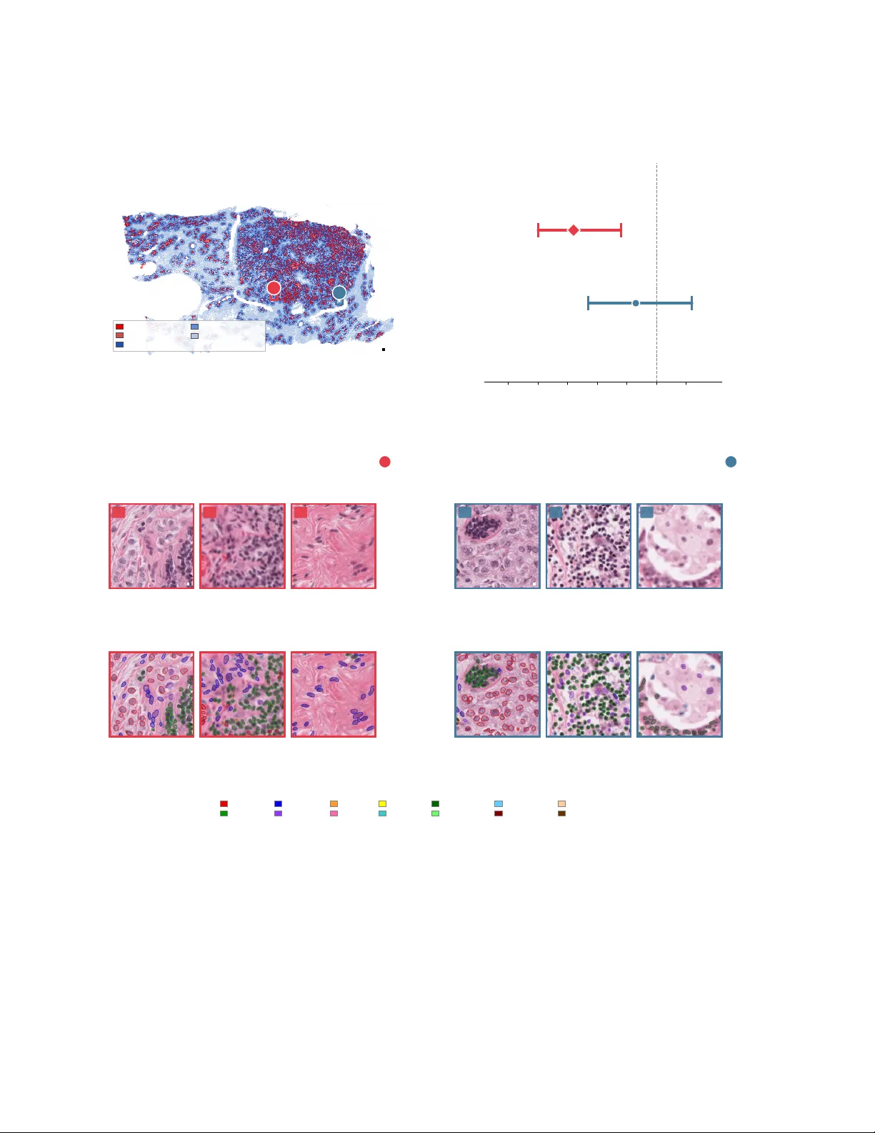
HistoAtlas: A Pan-Cancer Mor phology Atlas Linking Histomics to Molecular Pr ograms and Clinical Outcomes Pierre-Antoine Bannier W e present HistoAtlas, a pan-cancer computational atlas that extracts 38 interpretable histomic featur es from 6,745 diag- nostic H&E slides across 21 TCGA cancer types and systemat- ically links every feature to surviv al, gene expression, somatic mutations, and immune subtypes. All associations are covariate- adjusted, multiple-testing corrected, and classified into evidence- strength tiers. The atlas r ecovers known biology , from immune infiltration and prognosis to proliferation and kinase signaling, while uncov ering compartment-specific immune signals and mor - phological subtypes with diver gent outcomes. Every result is spatially traceable to tissue compartments and indi vidual cells, statistically calibrated, and openly queryable. HistoAtlas enables systematic, large-scale biomarker disco very from r outine H&E without specialized staining or sequencing. Data and an interac- tive web atlas ar e freely av ailable at https://histoatlas.com . Keyw ords: digital pathology , computational pathology , cancer his- tomics, tumor morphology , pan-cancer atlas, whole slide image, tumor microen vironment Correspondence: pierreantoine.bannier@gmail.com 1 Intr oduction Histopathological e xamination of hematoxylin-and-eosin- stained (H&E) tissue sections remains the gold standard for cancer diagnosis ( 1 , 2 ). Every diagnostic slide encodes quanti- tati ve information, from cell densities and nuclear morphology to spatial or ganization of immune infiltrates and stromal archi- tecture ( 3 ). In existing pan-cancer resources, this information is collapsed into categorical grades or discarded entirely ( 4 ). Genomics ( 5 ), transcriptomics ( 6 ), proteomics ( 7 ), and epige- nomics ( 8 ) each hav e mature pan-cancer resources that enable systematic cross-cancer comparison. Y et, histopathology , the most routinely generated cancer data modality , lacks an equiv alent quantitative atlas. The Cancer Genome Atlas (TCGA) established the paradigm for multi-omic inte gration across cancer types, cataloging somatic mutations, copy-number alterations, gene expression programs, and epigenetic landscapes ( 9 ). Thorsson et al. extended this framework to immune biology , defining six immune subtypes that stratify prognosis across 33 can- cer types using transcriptomic and genomic features ( 10 ). Nonetheless, neither resource incorporates quantitati v e mor- phological data. This is a notable omission because the spatial context of immune infiltration carries prognostic informa- tion independent of molecular subtyping, as formalized in the Immunoscore ( 11 – 13 ). Saltz et al. mapped bulk tumor infiltrating lymphocyte (TIL) density across 13 TCGA cancer types from deep-learning spatial maps ( 14 ), demonstrating the feasibility of pan-cancer morphological analysis from H&E. Howe ver , their approach reports a single bulk density score without compartment-specific resolution or linkage to gene expression programs. Computational pathology has made rapid progress in ex- tracting quantitati ve features from digitized slides ( 1 ). Early morphometric studies demonstrated that automated image features carry prognostic v alue in indi vidual cancer types ( 15 – 17 ). Deep-learning classifiers now predict molecular alter- ations ( 18 – 20 ), microsatellite instability ( 21 , 22 ), gene expres- sion ( 23 ), and surviv al ( 24 ) directly from H&E with high accu- racy . More recently , foundation models such as UNI ( 25 ), V ir- chow ( 26 ), or H0 ( 27 ), trained on large datasets of pan-tumor tissue via self-supervised learning, produce information-rich slide embeddings. Y et, these embeddings do not readily de- compose into interpretable biological features such as cell den- sities, spatial distances, or tissue compartment fractions ( 4 ). In response to this interpretability gap, se veral groups ha ve pro- posed explicit feature-based representations: Diao et al. ( 28 ) combined cell- and tissue-le vel predictions into hundreds of human-interpretable descriptors, and Abel et al. ( 29 ) deriv ed large collections of nuclear morphometric features linked to genomic instability and prognosis. These studies show that interpretable H&E features carry rich biological signal, but their emphasis on large feature spaces does not naturally orga- nize into a concise morphology atlas grounded in a small set of reproducible, compartment-resolved features. Public resources mirror this gap: cBioPortal provides molecular data without morphology ( 30 ), TCIA hosts raw slides without precomputed features ( 31 ), and the Human Pro- tein Atlas maps protein expression without quantitati ve mor- phometrics ( 32 ). These gaps leav e cancer researchers without a resource that bridges morphology and molecular biology at pan-cancer scale. Such a resource would need to com- bine interpretable histomic features with systematic molecular linkage across cancer types, e xplicit multiple-testing control, and traceability from statistical associations back to tissue compartments and individual cells. Here we present HistoAtlas, a pan-cancer morphology at- las built from 38 quantitati ve histomic features extracted from 6 , 745 TCGA diagnostic slides across 21 cancer types (plus a pooled pan-cancer analysis). W e systematically test ev ery fea- ture for association with surviv al, gene expression, mutations, copy-number variation, and immune subtypes with explicit correction families and evidence-strength badges (strong, mod- 1 erate, suggestiv e, or insufficient). All results are released as a web atlas in which e very association is spatially traceable to specific tissue compartments and individual cells (Fig. 6 ). W e demonstrate that resolving immune cells by tissue compart- ment uncov ers a stronger protective observ ational association between intratumoral lymphocyte density and survival than its stromal counterpart, a distinction diluted in bulk H&E- deriv ed TIL scoring approaches. Among morphologically dis- tinct clusters, morphology separates quiescent from hormone- driv en subgroups with di ver gent outcomes. 2 Results 2.1 A quantitative atlas of cancer mor phology W e constructed HistoAtlas from 6 , 745 H&E-stained diag- nostic slides spanning 21 TCGA solid-tumor cancer types (Supplementary T able 3). T welve additional cancer types were excluded because their dominant cell morphologies (lym- phoid, glial, melanocytic, mesench ymal, neuroendocrine, re- nal tubular , or germ cell) fall outside the training domain of the segmentation models (Supplementary T able 3). T wo automated segmentation stages con verted whole-slide images into quantitati ve measurements (§ 4.2 ). First, a UNet- based tissue segmentation model classified approximately 1.4 m 2 of tissue into fi ve compartments (tumor [mean 44.9% of tissue area], stroma [45.4%], necrosis, blood, and normal epithelium; Fig. 1 a), with tumor and stroma together account- ing for o ver 90% of the analyzed area. Second, the HistoPLUS cell detection and classification model ( 33 ) identified more than 4.4 billion individual cells belonging to nine types: tu- mor cells, lymphocytes, fibroblasts, neutrophils, eosinophils, plasmocytes, apoptotic bodies, mitotic figures, and red blood cells. From these segmentations we derived 38 histomic fea- tures org anized into fi ve cate gories: tissue composition, cell densities, nuclear morphology and kinetics, spatial or ganiza- tion, and spatial heterogeneity (definitions in Supplementary T able 1; descriptive statistics in Supplementary T able 10 ; pre- processing in § 4.3 ). W e then tested each feature for associations with surviv al and molecular programs across all 22 cohorts. For surviv al, we fitted Cox proportional-hazards models for each combination of 38 features, 22 cohorts (21 cancer types plus a pan-cancer cohort), and four endpoints (overall, disease-specific, disease- free, and progression-free surviv al), yielding 5 , 623 ev aluable associations (of a theoretical maximum of 6 , 688 ; the remain- der were excluded for insuf ficient sample size or e vents) un- der two adjustment tiers, unadjusted and adjusted for age, sex, stage, and tissue source site (§ 4.4 ). After Benjamini– Hochberg correction within predefined correction families (§ 4.9 ; Supplementary T able 6), 260 associations were signif- icant at a false discov ery rate of 0.05. All 260 passed the proportional-hazards assumption (Schoenfeld P ≥ 0 . 05 ; Sup- plementary T able 7), because associations with PH violations hav e their Cox P -values in validated before BH correction (§ 4.4 ); restricted mean survi val time (RMST) summaries are provided as complementary measures for all associations. For molecular associations, we computed 487 , 638 Spear- man rank correlations between 38 histomic features and 293 molecular targets, comprising 133 curated cancer genes assessed for both mRN A expression and cop y-number varia- tion (Supplementary T able 4), 21 Hallmark pathway acti vity scores (of the 50 Hallmark gene sets, 21 had sufficient matched data), and 6 immune cell-fraction scores, across 22 cohorts under two adjustment tiers (§ 4.5 ). After family- wise Benjamini–Hochberg correction (Supplementary T a- ble 6), 88 , 920 correlations (18.2%) were significant at a false discov ery rate of 0.05, with the highest yield among immune cell fractions (39.2%), pathway scores (30.4%), and gene expression (24.9%), and the lo west among copy-number v ariation (6.3%) (Supplementary T able 11 ). Sample sizes v ary across analyses because not all slides have matched molecular or clinical annotation; exa ct counts are reported per analysis throughout. The following subsections present what these as- sociations show , beginning with a pan-cancer morphological landscape and progressing to compartment-resolv ed surviv al signals. 2.2 The pan-cancer morphological landscape reco vers canonical biology Our pipeline e xtracts 38 quantitati ve histomic features from each diagnostic H&E slide through automated tissue segmen- tation, cell detection, and spatial analysis (Fig. 1 a). Pair - wise Spearman correlation across all 6 , 745 slides revealed structured feature modules – density features form a tight positiv e-correlation block, morphology features cluster to- gether , and cross-module anti-correlations delineate distinct biological axes (Fig. 1 b) – confirming that the 38 features cap- ture complementary aspects of tissue biology . T o visualize the morphological landscape, we projected all 6 , 745 slides into a two-dimensional UMAP embedding computed from these fea- tures (§ 4.7 ; Fig. 1 c). Cancer types occupied distinct regions of the embedding, with morphologically related types positioned adjacently: squamous carcinomas (HNSC, LUSC, CESC) clustered in a region of elev ated nuclear pleomorphism, while hormone-driv en adenocarcinomas (BRCA, PRAD) occupied a low-proliferation re gion. Unsupervised K-means clustering of the z-scored feature vector , without any molecular input, yielded 10 pan-cancer (L1) clusters ( K selected by inspection of silhouette, Calinski–Harabasz, Davies–Bouldin, and gap statistic metrics; § 4.7 ; Fig. 1 d,e) and 69 cancer -specific (L2) subclusters. Bootstrap stability analysis (50 iterations, 80% subsamples) confirmed rob ust cluster assignments (mean ad- justed Rand index = 0 . 72 , Jaccard = 0 . 81 ). The adjusted Rand index between L1 clusters and cancer-type labels was 0.15, confirming that the clusters capture morphological v ariation that is not reducible to cancer-type identity . Pathway and immune subtype enrichment analysis re- 2 vealed that these purely morphological clusters align with canonical molecular programs (§ 2.5 ). All pathway enrich- ments belo w are Cliff ’ s δ computed on Hallmark gene set scores ( 34 ) (Supplementary T able 5 ). Cluster 4 (76% THYM) exhibited strong immune rejection pathway enrich- ment ( δ = 0 . 67 , 95% CI [ 0 . 60 , 0 . 73 ] , P adj = 3 . 3 × 10 − 40 ), consistent with the activ e T -cell maturation en vironment that defines thymic biology ( 35 , 36 ). Cluster 6 (61% CO AD and READ) sho wed dominant Wnt/ β -catenin signaling ( δ = 0 . 46 , 95% CI [ 0 . 42 , 0 . 50 ] , P adj = 1 . 3 × 10 − 82 ) and C1 wound-healing immune subtype enrichment (OR = 5 . 59 , 95% CI [ 4 . 69 , 6 . 67 ] , P adj = 1 . 1 × 10 − 88 ), recapitulating the constitutiv e WNT acti v ation that characterizes colorectal tumorigenesis ( 37 ). Cluster 8 (44% BRCA, 24% PRAD) displayed estrogen response upregulation ( δ = 0 . 52, 95% CI [ 0 . 49 , 0 . 56 ] , P adj = 2 . 2 × 10 − 160 ) and proliferation suppression ( δ = − 0 . 51 , 95% CI [ − 0 . 54 , − 0 . 48 ] , P adj = 3 . 8 × 10 − 154 ), consistent with the hormone-driv en, genomically quiet phe- notype of luminal breast and prostate cancers ( 9 , 38 ). The algorithm recei ved no molecular input, yet grouped th ymomas by immune rejection pathways, colorectal cancers by WNT activ ation, and hormone-driven tumors by estrogen response. Because L1 clusters dominated by a single cancer type could trivially inherit that type’ s molecular profile, we ex- amined two additional lines of e vidence. First, Cluster 3 ( n = 1 , 012 ) spans five cancer types with no dominant con- tributor (HNSC 17.7%, ST AD 17.2%, BLCA 14.3%, LUSC 14.3%, LUAD 11.8%) yet sho wed coherent enrichment for hypoxia ( δ = 0 . 34 , 95% CI [ 0 . 30 , 0 . 38 ] , P adj = 1 . 7 × 10 − 57 ), interferon- γ response ( δ = 0 . 46 , 95% CI [ 0 . 43 , 0 . 49 ] , P adj = 1 . 3 × 10 − 105 ), and C2 (IFN- γ dominant) immune subtype (OR = 2 . 74 , 95% CI [ 2 . 37 , 3 . 17 ] , P adj = 2 . 1 × 10 − 40 ). Second, within-cancer (L2) subclusters sho wed biology beyond cancer- type identity: within BRCA alone, subcluster 2 ( n = 280 ) was enriched for C2 immune subtype (OR = 4 . 86 , 95% CI [ 3 . 58 , 6 . 59 ] , P adj = 8 . 1 × 10 − 25 ) and interferon- γ response ( δ = 0 . 47 , 95% CI [ 0 . 39 , 0 . 54 ] , P adj = 3 . 8 × 10 − 28 ), while subcluster 3 ( n = 325 ) showed estrogen response enrichment ( δ = 0 . 26 , 95% CI [ 0 . 19 , 0 . 34 ] , P adj = 1 . 2 × 10 − 9 ) and deple- tion across all six immune pathways. These within-cancer results confirm that the histomic features capture biological heterogeneity not reducible to cancer-type identity . The re- maining clusters and their surviv al associations are detailed in § 2.5 . 2.3 Spatial immune topology is associated with surviv al in a compartment-specific manner Unlike bulk TIL scoring approaches ( 14 , 39 ), HistoAtlas quan- tifies immune cell density , spatial proximity , and infiltration patterns separately in the intratumoral, stromal, and in vasi ve front compartments. All surviv al associations in this sub- section use Cox regression adjusted for age, sex, stage, and stratified by tissue source site for o verall survi v al (§ 4.4 ; pan- cancer models additionally stratified by cancer type). Pan-cancer analysis re vealed compartment-specific dif fer - ences in prognostic strength (Fig. 2 a). Intratumoral lympho- cyte density was associated with fav orable outcomes (pan- cancer hazard ratio [HR] = 0 . 87 , 95% CI [ 0 . 81 , 0 . 93 ] , P adj = 9 . 8 × 10 − 4 , n = 4 , 560 ), whereas stromal lymphocyte density showed a weaker , attenuated protectiv e effect (HR = 0 . 89 , 95% CI [ 0 . 83 , 0 . 97 ] , P adj = 0 . 031 , n = 4 , 561 ). Intratumoral lymphocyte density sho wed a protectiv e direction (HR < 1 ) in 11 of 17 ev aluable cancer types, with BRCA exhibiting the strongest effect (HR = 0 . 72 , 95% CI [ 0 . 60 , 0 . 88 ] , P adj = 0 . 018 , n = 960 ; Fig. 2 b) followed by HNSC (HR = 0 . 74 , 95% CI [ 0 . 63 , 0 . 87 ] , P adj = 3 . 9 × 10 − 3 , n = 444 ). In BRCA, stromal lymphocyte density sho wed a weaker , non-significant associa- tion (HR = 0 . 93 , 95% CI [ 0 . 77 , 1 . 12 ] , P adj = 0 . 67 ), indicating that the intratumoral compartment carries the dominant prog- nostic signal (Fig. 6 b). Aggregate TIL scores that combine both compartments dilute this compartment-specific effect. Spatial proximity features provided an additional prog- nostic axis. Tumor -lymphocyte nearest-neighbor distance at the in vasi ve front, a spatial measure of immune exclu- sion ( 40 , 41 ), in versely correlated with CD8A expression in BRCA ( ρ = − 0 . 53, P adj = 1 . 8 × 10 − 68 , n = 958; Fig. 2 c). Gene-lev el correlations validated the biological identity of these features. In BRCA, intratumoral lymphocyte density correlated with cytotoxic T -cell markers and immune check- point genes (CD8A: ρ = 0 . 59 , 95% CI [ 0 . 54 , 0 . 63 ] ; TIGIT : ρ = 0 . 63 , 95% CI [ 0 . 59 , 0 . 67 ] ; both P adj < 10 − 85 , n = 958 ; Fig. 2 d). These features also discriminated Thorsson immune subtypes ( 10 ): peritumoral immune richness (the number of distinct immune cell types detected within 50 µm of the tu- mor boundary; Supplementary T able 1) explained 13% of immune subtype variance (Kruskal–W allis η 2 = 0 . 13 , 95% CI [ 0 . 12 , 0 . 15 ] , P adj = 3 . 0 × 10 − 159 , n = 5 , 590 ; pan-cancer), consistent with concordance between histomic and transcrip- tomic immune classifications. A composite feature, interface- normalized immune pressure (lymphoc yte count within 50 µm of the tumor–stroma boundary divided by interface length, cells mm − 1 ; Supplementary T able 1), was protecti ve in HNSC (HR = 0 . 74 , 95% CI [ 0 . 63 , 0 . 86 ] , P adj = 3 . 9 × 10 − 3 , n = 444 ; a value similar to intrat umoral lymphocyte density , reflecting the high correlation between these features). Additional features showed consistent protective trends across cancer types. L ymphocyte density spatial heterogeneity was protecti ve in 14 of 17 e valuable cancer types (unadjusted model). The unadjusted associations for interface-normalized immune pressure in BRCA (HR = 0 . 72 , P adj = 7 . 6 × 10 − 3 ) and LIHC (HR = 0 . 79 , P adj = 0 . 038 ) did not survi ve cov ariate adjustment. 2.4 Morphometric featur es encode molecular programs W e next tested whether purely morphometric features serve as proxies for molecular programs. Of the 487 , 638 histomic– molecular correlations (§ 2.1 ), 88 , 920 (18.2%) were significant 3 at FDR < 0 . 05 . Under a permutation null model (100 shuffles of molecular labels within each cancer type, with per -cancer- type BH correction matching the production pipeline), 0% of pairs were significant at the same threshold, confirming that the observed 18.2% discov ery rate reflects genuine biological signal rather than statistical artifact (Supplementary Methods). The correlation structure was biologically coherent: immune density features correlated with immune pathway signatures, proliferation features with cell c ycle pathways, and in vasion features with epithelial-mesenchymal transition (EMT) scores (Fig. 3 a). Among significant pairs, the median absolute ρ was 0.18 (IQR 0.13–0.27). Fig. 3 b shows the distribution of ef fect sizes for pan-cancer adjusted-model associations, stratified by molecular data type: gene expression ( 4 , 371 / 5 , 453 sig- nificant, 80%), Hallmark pathways ( 1 , 692 / 2 , 050 , 83%), and copy-number v ariation (2 , 845/5 , 453, 52%). Three examples from breast cancer (BRCA, n = 958 ; un- adjusted model) illustrate the strength of this morphology- to-molecular correspondence. First, mitotic index correlated with canonical proliferation markers (PLK1: ρ = 0 . 56 , 95% CI [ 0 . 51 , 0 . 61 ] , P adj = 5 . 2 × 10 − 77 ; additional markers in- cluding A URKA, MKI67, CCNB1, and TOP2A). Second, in v asion depth showed modest correlations ( | ρ | = 0 . 25 – 0 . 32 ) consistent with the classical EMT axis ( 42 ), with ZEB1 as the strongest correlate ( ρ = 0 . 32 , 95% CI [ 0 . 26 , 0 . 37 ] , P adj = 8 . 4 × 10 − 23 ) and an inv erse correlation with the epithelial marker CDH1 ( ρ = − 0 . 25 , 95% CI [ − 0 . 32 , − 0 . 19 ] , P adj = 1 . 0 × 10 − 14 ). Third, nuclear pleomorphism anti-correlated with luminal dif ferentiation markers (BCL2: ρ = − 0 . 37 , 95% CI [ − 0 . 43 , − 0 . 32 ] , P adj = 8 . 1 × 10 − 32 ; ESR1: ρ = − 0 . 36 , 95% CI [ − 0 . 41 , − 0 . 30 ] , P adj = 4 . 4 × 10 − 29 ), consistent with the histological grading criteria of Elston and Ellis ( 43 ). The mitotic index–PLK1 correspondence generali zed across can- cer types (LU AD: ρ = 0 . 65 , n = 437 ; LIHC: ρ = 0 . 60 , n = 348; pan-cancer: ρ = 0 . 68, n = 5 , 875; all P adj < 10 − 27 ). In v asion depth also in versely correlated with cell cycle pathway scores in BRCA ( ρ = − 0 . 30 , 95% CI [ − 0 . 36 , − 0 . 25 ] , P adj = 4 . 6 × 10 − 21 , n = 957 ). This slide-lev el in verse associ- ation between inv asion and proliferation is consistent with the “go-or-grow” hypothesis ( 44 , 45 ), although it cannot establish single-cell-lev el mutual exclusi vity . T ogether , these correspondences confirm that histomic features capture in- terpretable aspects of kno wn biological programs, providing a morphology-to-molecular bridge that operates without specialized staining or sequencing. 2.5 Morphological clusters define molecular archetypes Beyond the pathway enrichments that independently re- cov ered canonical biology (§ 2.2 ), the 10 L1 clusters also carried distinct mutational and immune subtype profiles (Fig. 4 a,b). Mutation enrichment analysis (Fisher’ s ex- act test, FDR < 0 . 05 ) showed Cluster 6 (61% CRC) en- riched for TTN (odds ratio [OR] = 1 . 91 , 95% CI [ 1 . 58 , 2 . 31 ] , P adj = 1 . 4 × 10 − 9 ), F A T4 (OR = 1 . 91 , 95% CI [ 1 . 46 , 2 . 49 ] , P adj = 4 . 9 × 10 − 5 ), and SYNE1 (OR = 1 . 86 , 95% CI [ 1 . 47 , 2 . 35 ] , P adj = 1 . 1 × 10 − 5 ), mutations frequently ob- served in colorectal genomes. Cluster 8 (44% BRCA, 24% PRAD) was depleted for chromatin modifier mutations (KMT2D OR = 0 . 42 , 95% CI [ 0 . 31 , 0 . 55 ] , P adj = 5 . 8 × 10 − 11 ; ZFHX4 OR = 0 . 44 , 95% CI [ 0 . 33 , 0 . 58 ] , P adj = 4 . 8 × 10 − 10 ), consistent with a genomically quiet, hormone-dri ven pheno- type. Because cluster molecular enrichments partly reflect cancer-type composition (e.g., Cluster 4 is 76% THYM), within-cancer-type (L2) enrichments that control for this confound are av ailable in the web atlas. Cluster-le v el surviv al analysis used Cox re gression strati- fied by cancer type (Fig. 1 d). This analysis revealed a prog- nostically important distinction among morphologically dis- tinct clusters. Cluster 2 ( n = 607 ; 44% LIHC, 28% THCA) displayed profoundly quiescent morphology: proliferation pathway scores were suppressed relative to all other slides (Cliff ’ s δ = − 0 . 58 , P adj = 4 . 2 × 10 − 102 ; E2F targets), and it showed fa v orable surviv al (HR = 0 . 54 , 95% CI [ 0 . 40 , 0 . 73 ] , P adj = 6 . 3 × 10 − 4 ; n = 516 with e vents). Cluster 5 ( n = 488 ; 25% A CC, 20% BRCA) showed immune spatial exclusion (de- pleted cytotoxic immune activity; Cliff ’ s δ = − 0 . 54 , P adj = 2 . 3 × 10 − 62 ; allograft rejection) with near -a verage prolifera- tiv e acti vity , and a non-significant adverse trend (HR = 1 . 17 , 95% CI [ 0 . 96 , 1 . 42 ] , P adj = 0 . 28). Thorsson immune subtype ( 10 ) composition further dis- tinguished the two clusters. Cluster 5 was enriched for C4 (lymphocyte depleted; OR = 5 . 49 , 95% CI [ 4 . 23 , 7 . 11 ] , P adj = 2 . 8 × 10 − 30 ; 28% of slides) and depleted for C2 (IFN- γ domi- nant; OR = 0 . 48 , P adj = 3 . 9 × 10 − 8 ). Cluster 2 showed com- bined C4 (OR = 7 . 14 , 95% CI [ 5 . 72 , 8 . 93 ] , P adj = 1 . 3 × 10 − 56 ) and C3 (inflammatory; OR = 4 . 99 , 95% CI [ 4 . 13 , 6 . 02 ] , P adj = 1 . 6 × 10 − 60 ) enrichment (85% combined; Fig. 4 a). Although C3 is labeled “inflammatory , ” Cluster 2’ s morphology was uniformly quiescent, with suppressed lymphocyte density and proliferativ e indices, suggesting that its C3-classified tumors represent a quiescent inflammatory state rather than active immune engagement. Immune subtype labels alone classified both clusters as immune-depleted v ariants b ut did not distin- guish their div ergent proliferativ e states; the morphological axis of quiescent-cold versus hormone-driven tumors added prognostic information that transcriptomic subtyping did not capture. Cluster 8 (BRCA/PRAD, hormone-driv en) showed ad- verse survi v al (HR = 1 . 37 , 95% CI [ 1 . 15 , 1 . 62 ] , P adj = 1 . 8 × 10 − 3 , n = 1 , 112 ). The remaining clusters did not reach signif- icance after BH correction. Hazard ratios and P -values for all 10 clusters are shown in Fig. 1 d. 2.6 Reporting what the atlas detects and what it cannot HistoAtlas accompanies ev ery association with Benjamini– Hochberg-corrected ( 46 ) P -values, bootstrap confidence in- 4 tervals, effect sizes, and evidence-strength badges (Fig. 5 ; statistical details in § 4.9 – 4.11 ). W e assessed batch effects from tissue source site (TSS) using principal variance component analysis (PVCA) ( 47 ) and silhouette scores. At the pan-cancer level, PVCA attributed 44.7% of feature variance to TSS, 32.7% to cancer -type iden- tity , and 22.6% to residual (Fig. 5 a). Because TSS is partially confounded with cancer type (most sites contribute primarily one cancer type), the 44.7% TSS component includes both genuine institutional variation and cancer -type-associated mor- phological differences. W ithin individual cancer types, where batch effects could confound feature–outcome associations, per-cancer -type batch variance ranged from 2.7% (ACC) to 29.1% (ESCA), and all 20 per-cancer silhouette scores by TSS were neg ativ e (range − 0 . 18 to − 0 . 0004 ; one cancer type [CHOL] was excluded from per-cancer batch QC due to insuf- ficient TSS di versity), indicating that no cancer type e xhibited TSS-driv en sub-clustering. Spearman correlation P -values use the analytical t -test approximation ( t = r p df / ( 1 − r 2 ) ; § 4.5 ), v alidated by near - perfect concordance with a permutation-based reference ( ρ > 0 . 999 , n = 282 , 278 pairs). As a calibration check, we veri- fied that raw P -values for the weakest-signal features (those with median effect size in the bottom quartile) followed an approximately uniform distrib ution, consistent with the null expectation. T o quantify what the atlas cannot detect, we computed the minimum detectable effect size (MDES) at 80% po wer for every analysis, using the Schoenfeld–Freedman approx- imation ( 48 , 49 ) for surviv al associations and the Fisher z - transform for correlations. MDES varies across cancer types because sample sizes and e v ent counts dif fer: well-powered cancer types such as BRCA ( n = 960 for OS, 135 ev ents) can detect hazard ratios as small as 1.62, whereas underpo wered types such as cholangiocarcinoma (CHOL, n = 36 ) require hazard ratios exceeding 3.75 (Fig. 5 b). Each association recei ves an e vidence-strength badge (strong, moderate, suggestiv e, or insufficient) computed from adjusted P -value, effect size magnitude, confidence inter- val width, and sample size (§ 4.11 ). Across 5 , 623 surviv al associations (38 features × 22 cohorts × 4 endpoints × 2 ad- justment tiers, excluding combinations with insufficient data), 33 (0.6%) achiev ed strong evidence, 167 (3.0%) moderate, 577 (10.3%) suggesti ve, and 4 , 846 (86.2%) insuf ficient. The predominance of insufficient e vidence reflects the limited sta- tistical po wer of smaller cohorts: most insufficient-e vidence pairs in volv e cancer types with n < 100 , where MDES ex- ceeds clinically meaningful thresholds (Fig. 5 b). The 33 strong and 167 moderate associations span multiple cancer types and all fiv e feature categories, pro viding a curated set of high-confidence findings. Cross-endpoint replication rates for DSS, DFS, and PFS are discussed in Supplementary Note 2. 3 Discussion HistoAtlas demonstrates that interpretable, spatially resolved histomic features extracted from routine H&E slides recapit- ulate canonical molecular programs, including proliferation kinase networks, EMT transcriptional ax es, and immune cell gene signatures (Fig. 3 ), while stratifying clinical outcomes across cancer types. The central advance is not any single association but the comprehensi ve, statistically transparent linking of 38 quantitativ e features to surviv al, gene expres- sion, mutations, and immune subtypes at pan-cancer scale. W e deliver this linking as an openly queryable resource. A systematic biological plausibility audit (Supplementary T able 2 ) decomposed atlas findings into 60 atomic claims and assessed each against the literature. Of these, 42 (70%) are well-established or supported by prior studies ( 11 – 13 , 42 , 44 , 45 , 50 – 54 ), 12 (20%) are novel b ut biologically plausible, 5 (8%) are nov el with uncertain mechanisms, and 1 (2%) is an apparent contradiction that was resolved upon examination: spatial composition heterogeneity does not equate to genetic clonal div ersity ( 55 ) (Supplementary T able 2 ). No claim con- tradicted established biology , a necessary consistency check for the feature extraction and statistical frame work. Sev eral atlas-enabled findings warrant tar geted follow-up. The compartment-specific difference in prognostic strength between intratumoral and stromal lymphocyte density (strong versus weak protection, respectiv ely; Fig. 2 a) is consistent with the importance of immune cell localization within the tumor microen vironment ( 13 , 40 , 41 , 56 ). Saltz et al. scored bulk TIL density across 13 TCGA cancer types from deep- learning maps ( 14 ) but did not distinguish intratumoral from stromal compartments. T o our knowledge, the differential prognostic contribution of these compartments had not been quantified across 21 cancer types from H&E morphometrics. W e also identified morphologically distinct clusters with di- ver gent survi val outcomes: quiescent-cold (Cluster 2; hazard ratio = 0 . 54 ) versus hormone-driv en (Cluster 8; hazard ra- tio = 1 . 37 ; Fig. 1 d). This finding suggests that the binary immune-hot/immune-cold classification ( 56 ) may obscure bi- ologically and potentially clinically rele vant heterogeneity . Additional novel features showed consistent prognostic sig- nals: lymphocyte density spatial heterogeneity (coefficient of v ariation across tiles) was protecti ve in 14 of 17 e v aluable cancer types (unadjusted model) and may proxy tertiary lym- phoid structure formation ( 57 ); interface-normalized immune pressure, a composite measure of immune cell engagement at the tumor-stroma boundary , was protecti ve in HNSC (hazard ratio = 0 . 74 , P adj = 3 . 9 × 10 − 3 ); the unadjusted associations previously observed in BRCA and LIHC did not survive co- variate adjustment. TCGA lacks immunotherapy response data, so the clinical relev ance of these immune distinctions for treatment selection remains speculati ve. All findings are hypothesis-generating; none should be interpreted as estab- lished biomarkers without independent confirmation. Evaluating these findings in context requires comparing HistoAtlas to existing cancer data resources. cBioPortal ( 30 ) 5 provides comprehensi ve molecular and clinical data but lacks any morphological features. The Human Protein Atlas ( 32 ) provides semi-quantitativ e protein expression scores from immunohistochemistry with cancer-specific surviv al associ- ations ( 58 ), but does not extract continuous morphometric features from H&E-stained sections or link them to molec- ular programs beyond single-protein correlations. The Can- cer Imaging Archiv e ( 31 ) hosts raw imaging data without a statistical layer . Individual computational pathology stud- ies hav e linked H&E features to outcomes in single can- cer types ( 15 , 16 ), and Diao et al. extracted 607 human- interpretable features across fi ve cancer types ( 28 ), but most recent approaches rely on deep-learning embeddings that do not decompose into named histological features ( 25 , 26 ). His- toAtlas addresses this interpretability gap: a tissue segmenta- tion ov erlay with nine spatial zones deriv ed from fiv e tissue compartments, and cell-type annotations for nine morpholog- ical cell types enable users to trace any statistical finding to specific tissue regions and verify the underlying cell predic- tions visually (Fig. 6 a–d). Three categories of limitation constrain the current at- las. Data scope: all 6 , 745 slides deriv e from TCGA, a ret- rospectiv e con v enience cohort with institutional selection bi- ases ( 59 ). W e include 21 of 33 av ailable cancer types; the 12 excluded types harbor dominant cell populations (lymphoid, glial, melanocytic, mesenchymal, neuroendocrine, renal tub u- lar , or germ cell) outside the segmentation model’ s training domain (Supplementary T able 3). TCGA participants are pre- dominantly of European ancestry ( 9 , 59 ); generalizability to div erse populations remains untested. T reatment standards hav e ev olved since TCGA accrual (2000–2016), limiting appli- cability to contemporary regimens. F eature quality: because 13 of 21 cancer types are out-of-distribution for the cell se g- mentation model (trained on eight cancer types; § 4.2 ), feature reliability varies across the atlas, and certain cancers ( PRAD, LIHC, THCA) show elev ated mitotic and apoptotic indices from reduced cell detection. Sev en ratio features required win- sorization to mitigate gate loophole artif acts, distance features are quantized at 8 µm px − 1 resolution, and two tissue-model features carry zero signal. W e use one slide per case, sacri- ficing assessment of intratumoral heterogeneity . Analytical constraints: all surviv al models test one histomic feature at a time alongside clinical co variates; a penalized multiv ariate model (e.g., LASSO Cox) would identify which features carry independent prognostic information and is a natural next step. Sev eral features are correlated by construction (e.g., density features sharing the same denominator re gion), so the effecti ve number of independent features is lower than 38. Morphology- to-molecular correlations are modest in magnitude (median significant | ρ | = 0 . 18 , IQR 0 . 13 – 0 . 27 ); the features serve as noisy proxies for, not replacements of, molecular mea- surements. V alidation gap: we have not performed e xternal replication. All associations are internal to TCGA, and in- dependent confirmation in CPT A C ( 7 ) or MET ABRIC ( 60 ) cohorts is required before any clinical interpretation. W e hav e not benchmarked interpretable features against whole-slide foundation model embeddings ( 25 , 26 ); a direct comparison of predictiv e po wer versus interpretability would strengthen the case for handcrafted features but requires a dedicated study . Three extensions would substantially strengthen the atlas. Overlaying spatial transcriptomics data (V isium, MERFISH) onto histomic features would pro vide gold-standard validation for spatial immune metrics and could calibrate morphome- tric proxies against measured transcript distributions. Inte- grating foundation model embeddings alongside interpretable histomic features would enable direct comparison of inter- pretability versus predicti ve po wer . Extending the framework to non-TCGA cohorts would test generalizability and enable community-contributed cancer types. W e designed HistoAtlas for transparency and reuse. Every association carries an e vidence-strength badge (strong, mod- erate, suggesti ve, or insuf ficient) computed from adjusted P values, effect sizes, confidence interval widths, and sample sizes. The atlas reports the minimum detectable effect size at 80% po wer , con veying not only what it finds but also what it cannot detect. Bidirectional spatial traceability links ev ery population-le vel statistic to tissue compartment maps and indi- vidual cell annotations on the original slide, and from any slide back to population-le vel associations (Fig. 6 c,d). By making ev ery morphological association traceable, statistically cali- brated, and openly queryable by humans and machines alike, HistoAtlas provides infrastructure for systematic morphology- aware cancer analyses. All analysis code, feature metadata, and precomputed results are publicly released. 4 Methods 4.1 Data acquisition W e obtained formalin-fixed, paraffin-embedded (FFPE) hema- toxylin and eosin (H&E)-stained diagnostic whole-slide im- ages from The Cancer Genome Atlas (TCGA) via the Ge- nomic Data Commons (GDC) portal for 21 solid-tumor can- cer types (Supplementary T able 3). Slides were excluded if the viable tissue area fell belo w 1 mm 2 , if se vere processing artifacts (pen marks covering > 20% of tissue area, out-of- focus regions) were present, or if essential clinical metadata (vital status, follo w-up time) was missing. T o av oid pseudo- replication, we retained one slide per case: for each case with multiple diagnostic slides, we selected the primary tumor diagnostic slide with the largest tissue area, yielding 6 , 745 slides across 6 , 745 unique patients. T welve additional TCGA cancer types were excluded because their dominant cell mor- phologies fall outside the training domain of the cell detection model (Supplementary T able 3). Matched clinical data (ov erall surviv al, disease-specific surviv al, disease-free surviv al, and progression-free survi val; age at diagnosis, sex, pathologic stage, tissue source site [TSS], and tumor purity estimates) were obtained from the TCGA Pan-Cancer Clinical Data Resource (TCGA- 6 CDR) ( 59 ). Molecular data included RNA-seq gene expres- sion (RSEM normalized), somatic mutations from the MC3 multi-caller ensemble ( 61 ), copy-number v ariation, immune cell fraction estimates from CIBERSOR T ( 62 ) and xCell ( 63 ), tumor purity from ABSOLUTE ( 64 ), and immune subtype classifications (C1–C6) from Thorsson et al. ( 10 ). All molec- ular data were retrie ved from the GDC and P anCancerAtlas data repositories. Molecular data were matched to slides by TCGA case barcode (first 12 characters of the barcode); for cases with multiple aliquots, the primary tumor aliquot was selected. Thorsson immune subtype labels (C1–C6) were matched to slides by TCGA case barcode. Of 6 , 745 slides, 5 , 590 (82.9%) had matched immune subtype data; C5 (immunologically quiet, n = 65 ) and C6 (TGF- β dominant, n = 27) were retained but had limited statistical power . 4.2 F eature extraction W e computed 38 quantitativ e histological-morphometric (here- after “histomic”) features per slide, organized into fiv e cat- egories: tissue composition (3 features), cell densities (6), nuclear morphology and kinetics (8), spatial or ganization (18), and spatial heterogeneity (3). Complete definitions, units, and category assignments are pro vided in Supplementary T able 1 . Feature extraction used tw o segmentation stages. T issue segmentation used a CellV iT -inspired architecture ( 65 ) with a Phikon self-supervised V iT -B backbone ( 66 ), trained on the PanopTILs cro wdsourced annotation dataset ( 67 ); model weights are av ailable in the code repository . W e performed inference at 0.5 µm/px on 224 × 224 pixel tiles with 32-pixel ov erlap; the final segmentation mask was obtained by ma- jority voting in overlap regions. The model classified each tile into nine tissue classes: cancerous epithelium, stroma, necrosis, normal epithelium, TILs, junk/debris, blood, other , and whitespace (mean intersection-o ver -union = 0.72 on the PanopTILs held-out test set; note that per-class IoU varied substantially , and necrosis and normal epithelium had near- zero recall in deployment, reflecting their rarity in the training set and in resected TCGA specimens). Follo wing the Interna- tional Immuno-Oncology Biomarker W orking Group recom- mendation ( 39 ), regions classified as TILs were reclassified as stroma before all do wnstream computation, yielding fiv e ef- fecti ve compartments: cancerous epithelium, stroma, necrosis, normal epithelium, and blood. Cell segmentation and classification used the HistoPLUS model ( 33 ), which detects and classifies indi vidual cells into nine morphological types: tumor cells, lymphoc ytes, fibrob- lasts, plasmocytes, neutrophils, eosinophils, red blood cells, apoptotic bodies, and mitotic figures (mean panoptic quality [PQ] = 0.509 across cell types; per-class PQ v aried from 0.28 to 0.73, with lowest performance on rare cell types such as eosinophils and apoptotic bodies). Inference was performed on 224 × 224 pixel tiles at 40 × magnification (0.25 µm/px) when av ailable, falling back to 20 × (0.50 µm/px); the major- ity of slides were scanned at 40 × . W e extracted tiles with a 64-pixel (16 µm) overlap margin; cells detected in over - lap regions were deduplicated via a union-find algorithm that merges instances whose centroids fall within 10 µm, corre- sponding approximately to the diameter of a typical epithelial nucleus. The cell model was trained on pathologist annota- tions from eight cancer types (LUAD, LUSC, BRCA, CO AD, BLCA, O V , P AAD, MESO); the remaining 13 included cancer types were processed in an out-of-distribution (OOD) setting. T issue–cell discordance (cells in a tissue-model tumor region not classified as cancer cells by the cell model) v aried from 0% to 12% across all cancer types, with the highest rate in P AAD (12.2%) despite being in-distrib ution, likely due to the dense desmoplastic stroma and small tumor glands characteristic of pancreatic ductal adenocarcinoma. OOD cancer types sho wed additional issues, including inflated kinetic indices in PRAD, LIHC, and THCA attrib utable to reduced cell-detection sen- sitivity . Red blood cells and plasmocytes were not used in feature computation. All spatial features were computed on compartment masks resampled to a common resolution of r = 8 µm/px by nearest-neighbor interpolation to ensure scanner -in variant boundary computation. Connected components belo w A min = 2 , 048 µm 2 ( ≈ 32 pixels at 8 µm/px, equi valent to approximately 5 × 5 cell diameters) were removed per com- partment before distance transform computation to prevent noisy segmentation fragments from inflating boundary lengths. Fiv e spatial bands were defined using the signed Euclidean distance transform d T from the tumor boundary , where the tumor boundary was defined as the outer contour of the can- cerous epithelium compartment mask at 8 µm/px resolution (positiv e inside tumor, negati ve outside): tumor front B 0-50 T ( 0 ≤ d T ≤ 50 µm), tumor core B > 50 T ( d T > 50 µm), stroma near B 0-50 S ( − 50 ≤ d T < 0 ), stroma far B 50-200 S ( − 200 ≤ d T < − 50 ), and necrosis ring R 0-100 Nec (within 100 µm of the necrosis bound- ary). The 50 µm front band corresponds to approximately fiv e cell diameters; the 200 µm stroma cutoff was chosen as a heuristic approximation of the attenuation range of immune in- filtration gradients, informed by spatial immune profiling stud- ies ( 14 , 68 ). W e classified slides into growth-pattern regimes based on the tumor front fraction ϕ = A ( B 0-50 T ) / A ( Ω T ) : mass-forming ( ϕ ≤ 0 . 5 ), intermediate ( 0 . 5 < ϕ ≤ 0 . 8 ), or infiltrativ e ( ϕ > 0 . 8 ). A macro-tumor mask obtained by morphological closing (disk radius ρ = 200 µm), used solely for computing the micro_interface_ratio QC metric, detected micro-interface dominance in infiltrati ve tumors. T wo additional features (normal epithelium area fraction and tumor –normal contact fraction, both dependent on normal epithelium detection, which the tissue model did not reliably identify) were excluded from the atlas entirely due to zero signal across all slides. Sev en ratio features were suscepti- ble to gate-loophole artifacts producing e xtreme values when denominators approached zero; these were mitigated by the winsorization step described belo w . Distance-based features (nearest-neighbor distances) were quantized at 8 µm/px reso- lution owing to the tile grid spacing. 7 4.3 F eature pr epr ocessing Preprocessing of the 38 histomic features proceeded in three steps. First, 22 features with heavy right-ske w (all cell densi- ties, ratio features, distance features, and heterogeneity mea- sures including coef ficients of v ariation) were log-transformed using log ( 1 + x ) . Second, all 38 features were winsorized at the 0.5th and 99.5th percentiles (computed per feature across the full cohort) to mitigate the influence of extreme v alues arising from segmentation artif acts. Global (pan-cohort) per- centiles were used because the tar get artifacts (segmentation failures and ratio instabilities) are present across cancer types, though at v arying rates (tissue–cell discordance ranges from 0% to 12% by cancer type). Per-cancer -type winsorization was not used because the small sample sizes of sev eral co- horts (e.g., CHOL, n = 38 ) would yield unreliable percentile estimates. Third, features were z -score standardized to zero mean and unit variance. The scope of standardization var - ied by analysis: UMAP embeddings and K -means clustering used global z -scores (across all n samples), Cox regression used per-cancer -type z -scores (so hazard ratios reflect per-SD effects within each cancer type), and Spearman correlations used no z -score standardization (rank-based). Missing values ( < 2% of entries across all features) were imputed with the column median prior to standardization. Raw (untransformed) values were retained for display in the web atlas interface; all statistical models and embeddings consumed preprocessed values. 4.4 Surviv al analysis W e assessed associations between each histomic feature and four surviv al endpoints (overall surviv al [OS; designated as the primary endpoint], disease-specific surviv al [DSS], disease- free survi val [DFS], and progression-free survi val [PFS]) us- ing uni variate Cox proportional hazards (PH) re gression, im- plemented with the lifelines Python package ( 69 ) (no L2 penalization; penalizer=0.0 ). Each model tests a single histomic feature (plus cov ariates); multi variate models incor - porating multiple features simultaneously are not included in the current atlas (see Discussion). F or each feature–cancer type–endpoint combination, we fitted tw o models: (1) unad- justed (feature only); and (2) adjusted (feature + age at diagno- sis + sex + pathologic stage as cov ariates, stratified by tissue source site [TSS]). TSS w as handled as a stratification variable in Cox models ( strata=[’tss’] in lifelines ), allo wing each site to have its own baseline hazard function without consuming degrees of freedom, the standard approach for multi-center studies ( 70 ). Hazard ratios (HR) were reported per one standard de viation increase in the preprocessed fea- ture v alue, with 95% W ald confidence intervals computed as exp ( ˆ β 1 ± Φ − 1 ( 0 . 975 ) · SE ( ˆ β 1 )) , where SE was deri ved from the observed Fisher information matrix. Pan-cancer analy- ses used stratified Cox regression with cancer type as an ad- ditional stratification variable ( strata=[’cancer_type’] in lifelines ), allowing each cancer type its own baseline hazard function while estimating a single shared regression coefficient. This approach av oids confounding by differential baseline hazard rates across cancer types. Per-cancer -type results constitute the primary analyses. Features and age were standardized (z-scored) prior to fitting; categorical covari- ates (sex, stage) were one-hot encoded with the first category dropped. F or the adjusted model, we used multiple impu- tation by chained equations (MICE) with a Bayesian ridge regression imputer ( scikit-learn IterativeImputer , 5 imputations, max 10 iterations per imputation, random seed incremented per imputation). Results were pooled using Ru- bin’ s rules, yielding combined hazard ratios, standard errors, and P -values; the fraction of missing information (FMI) was recorded for each analysis. When covariate missingness ex- ceeded 20% in an y v ariable, when total sample size was belo w 30, or when fewer than 3 of 5 imputations produced v alid fits, MICE was skipped and complete-case analysis was used as a fallback. Missingness arose primarily from incomplete staging annotations and varied by cancer type (Supplementary T able 8 ). A minimum sample size of n ≥ 30 with ≥ 10 ev ents was required per feature–cancer type–endpoint combination. Models were fitted only when the residual degrees of freedom remained positiv e after accounting for all cov ariates. W e tested the proportional hazards assumption for ev- ery fitted model using Schoenfeld residuals with the Kaplan– Meier time transform ( 71 ). The PH test P -value was used to flag each association: “pass” ( P ≥ 0 . 05 ), “warn” ( 0 . 01 ≤ P < 0 . 05 ), or “fail” ( P < 0 . 01 ). The P < 0 . 01 threshold for failure was chosen to balance sensitivity against the high multiple- testing burden (hundreds of models per cancer type); we note that this threshold has asymmetric po wer: large cohorts (e.g., BRCA, n ≈ 960 ) can detect trivial PH departures, whereas small cohorts (e.g., CHOL, n = 36 ) have limited power to detect e ven substantial violations. The prev alence of PH vio- lations across cancer types and endpoints is reported in Sup- plementary T able 7. When the PH assumption was violated ( P < 0 . 05 , encompassing both “warn” [ 0 . 01 ≤ P < 0 . 05 ] and “fail” [ P < 0 . 01 ] tiers), we inv alidated the Cox hazard ratio, confidence intervals, and P -value (set to NaN), as these quan- tities are unreliable under non-proportional hazards. For BH correction, in v alidated P -v alues were set to 1.0 to preserve the correction family size without inflating f alse discov eries. As a complementary , assumption-free summary , we additionally computed the restricted mean surviv al time (RMST) differ - ence. RMST was calculated as the area under the Kaplan–Meier curve up to a cancer-type-specific time horizon, with stan- dard errors estimated using the Irwin variance formula ( 72 ). The default horizon was 1 , 095 days (3 years). For aggressi ve cancer types with short median surviv al, we used a 2-year horizon (P AAD, MESO). F or indolent cancer types, we used a 5-year horizon (THCA, PRAD). These horizons were chosen to ensure adequate follow-up and at-risk populations at the truncation point; cancer-type-specific v alues are listed in Sup- plementary T able 9 . RMST differences between high and low 8 feature groups (median split) were tested using a permutation procedure ( 5 , 000 permutations of group labels). The median split was used for interpretability and consistency with the clinical con vention of risk stratification; we acknowledge that dichotomization discards information and reduces statistical power relative to continuous methods ( 73 ). P -values were computed as P = ( # { b : | ∆ b | ≥ | ∆ obs |} + 1 ) / ( B + 1 ) . Boot- strap confidence intervals (95%) for the RMST difference were obtained from 1 , 000 bootstrap resamples of the full co- hort, using the percentile method. RMST analyses required n ≥ 20 total subjects with ≥ 5 observations per group. For cluster-lev el surviv al comparisons, a two-sided log- rank test was computed between cluster members and non- members, with BH correction applied within each combina- tion of cluster lev el, analysis type, cancer type, and endpoint. 4.5 Molecular correlations W e computed Spearman rank correlations between each of the 38 histomic features and 293 molecular targets: 133 curated genes drawn from established cancer gene panels (OncoKB ( 74 ), COSMIC Cancer Gene Census ( 75 )), im- mune checkpoint targets (TIGIT , PD-L1, CTLA4, LAG3), and EMT/stemness markers curated from Nieto et al. ( 42 ) (complete list in Supplementary T able 4), each assessed for both expression and copy-number variation (133 × 2 = 266); 21 MSigDB Hallmark pathway scores ( 34 ) (of the 50 Hallmark gene sets [Supplementary T able 5 ], 21 had sufficient matched data after intersection filtering); and 6 immune cell fraction scores from CIBERSOR T ( 62 ). Pathway activity scores were computed via single-sample Gene Set Enrichment Analysis (ssGSEA; gseapy 1.1.12) ( 76 ) using the full TCGA Pan-Cancer batch-corrected RN A-seq expression matrix ( ∼ 20,500 genes per sample, EB++AdjustP ANCAN_ IlluminaHiSeq_RN ASeqV2 from UCSC Xena ( 77 )). The 50 Hallmark gene sets (median ∼ 200 genes per pathway) provide well-characterized, non-redundant representations of biological processes with established provenance ( 34 ). Gene sets with fewer than 10 genes present in the e xpression matrix after intersection were excluded (a stricter threshold than GSEA enrichment analysis below , because per-sample ssGSEA scores are noisier with small gene sets). For unadjusted models, we computed the standard Spear- man correlation coefficient and its analytical P -value ( t - approximation) using scipy.stats.spearmanr , which is accurate for n ≥ 10 and avoids the P -value banding that oc- curs with permutation floors. Bootstrap confidence interv als (95%) were obtained from 1 , 000 resamples using the per - centile method: for each resample, observations were dra wn with replacement, ranks recomputed, and the Spearman ρ recorded. For cov ariate-adjusted models, we computed partial Spearman correlations via the follo wing procedure: (1) rank- transform both the histomic feature and the molecular tar- get, as well as all cov ariates; (2) residualize the ranked feature and ranked target against the ranked cov ariates us- ing ordinary least-squares regression; and (3) compute the Pearson correlation of the residuals, yielding the partial Spearman ρ ( 78 ). P -values for partial correlations were obtained using the standard t -test for partial correlations: t = r p df / ( 1 − r 2 ) with df = n − 2 − k , where k is the number of cov ariate columns after one-hot encoding, and a two-sided P -value from the t ( df ) distribution. This matches the ap- proach used by R’ s ppcor::pcor.test() and Python’ s pingouin.partial_corr() . Bootstrap CIs for the par - tial Spearman ρ were obtained from 1 , 000 resamples, each recomputing the full rank–residualize–correlate pipeline. A cancer type was included in the correlation analysis if it contained n ≥ 30 samples; individual feature pairs required n ≥ 10 non-missing observations. All correlations were com- puted per cancer type. Deterministic per-task random seeds were deriv ed from a hash of the cancer type, histomic feature, and molecular feature names, ensuring reproducibility across parallel ex ecutions. In total, the correlation analysis comprised 487 , 638 histomic–molecular pairs: 38 features × 293 molecular tar- gets (133 genes × 2 data types [expression and copy number] + 21 Hallmark pathway scores + 6 immune cell scores) × 22 cohorts (21 cancer types + pan-cancer), each ev aluated under two adjustment models (unadjusted and adjusted [age, sex, stage, TSS]); the stated total e xcludes combinations with in- suf ficient data. TSS was included as a grouped co variate rather than a stratification variable because the rank-residualization procedure requires explicit cov ariate columns; TSS was grouped into the five most frequent sites per cancer type, with remaining sites collapsed to “Other”, to limit the number of dummy variables in the residualization. 4.6 Categorical associations Associations between histomic features and cate gorical molec- ular variables (somatic mutations [mutant vs. wild-type], copy- number alterations [amplification/deletion vs. neutral], and immune subtypes [C1–C6]) were tested separately for each cancer type. For unadjusted models, inference used the exact or asymp- totic distribution of the test statistic as implemented in scipy .stats . T wo-group comparisons used the Mann–Whitney U test (two-sided) with Cliff ’ s δ as the effect size. Cliff ’ s δ was computed as the mean of the sign matrix sign ( x i − y j ) ov er all n 1 × n 2 pairs, with 95% bootstrap CIs ( 1 , 000 resamples); bootstrap rather than analytical CIs were used because the data contain tied values, which violate the continuity assump- tion of Clif f ’ s analytical v ariance formula ( 79 ). For variables with more than two lev els, we used the Kruskal–W allis H test with η 2 H = ( H − k + 1 ) / ( N − k ) as the effect size ( 80 ), floored at zero. Bootstrap CIs for η 2 were obtained from 1 , 000 resamples of the group arrays. For cov ariate-adjusted models, we used rank-ANCO V A with Freedman–Lane permutation inference ( 81 ). The re- sponse (histomic feature) and all covariates were rank- 9 transformed. The group effect was tested by comparing the full model (group dummies + rank-transformed cov ari- ates) to the reduced model (cov ariates only) via an F -statistic on the residual sum of squares. P -values were obtained by permuting residuals from the covariate-only model ( 1 , 000 permutations). The F -statistic null distribution is parametri- cally smooth (approximately F -distributed under the null), requiring relatively few permutations for stable P -value es- timation; with 1 , 000 permutations the minimum achiev able P -value is ≈ 0 . 001 , sufficient for BH correction within the per-cancer -type families used here. The effect size was partial η 2 = SS group / ( SS group + SS residual ) . Bootstrap CIs for partial η 2 were computed from 1 , 000 resamples. Group ordering for binary comparisons followed a de- terministic con vention: mutant before wild-type, amplifica- tion/deletion before neutral. This ensured consistent sign interpretation of Cliff ’ s δ across analyses. A minimum of n ≥ 30 total observations and ≥ 5 observations per group w as required; groups smaller than 5 were excluded. 4.7 Clustering Unsupervised morphological clustering was performed in two tiers. At the L1 (pan-cancer) level, all 6 , 745 slides were clus- tered on the full 38-dimensional preprocessed feature v ector (after log-transform, winsorization, and z -scoring). At the L2 (cancer-specific) lev el, clustering was performed inde- pendently within each cancer type using cancer-type-specific z -scores. W e used K -means clustering ( scikit-learn , n init = 10 , random state fixed at 42). For L1, clustering was computed for K ∈ { 3 , . . . , 25 } ; silhouette, Calinski–Harabasz, Davies– Bouldin, and gap statistic scores were computed for each K . K = 10 was selected based on con ver gence of silhouette (local maximum at K = 10 ), Calinski–Harabasz (plateau), Da vies– Bouldin (local minimum), and gap statistic scores, balancing cluster interpretability against granularity (the gap statistic fa vored K = 8 ; silhouette fav ored K = 10 ). K -means was chosen for its scalability and interpretability; the resulting clusters should be understood as a con venient partition of feature space rather than a claim about the true number of distinct morphological subtypes. W e did not apply PCA di- mensionality reduction before clustering; the 38-dimensional feature space was used directly to preserve interpretability of cluster feature profiles. The effecti ve dimensionality (17 components explain 90% of v ariance) suggests moderate re- dundancy , which giv es correlated features proportionally more weight. For L2, the number of clusters was selected by the elbow method: we computed inertia for K values ranging from 2 to 8 (depending on cohort size) and selected the K that maximized the perpendicular distance from each point to the line connecting the first and last ( K , inertia ) points in the normalized space ( 82 ). Cancer types with fewer than 20 samples were assigned a single cluster without optimization. For cancer types with ≥ 20 samples, this yielded K ∈ [ 2 , 7 ] (69 L2 subclusters total). Individual clusters with fewer than 10 samples were e xcluded. Internal v alidation metrics (silhouette score, Calinski–Harabasz index, and Da vies–Bouldin inde x) were computed for each candidate K and reported alongside the selected solution. Cluster stability was assessed via repeated random subsam- pling: 50 iterations of 80% subsampling without replacement, re-clustering with the same K and n init = 10 , and comparison to the original labels using the adjusted Rand index (ARI) and mean best-match Jaccard index across clusters ( 83 ). The 50-iteration count provides sufficient precision for stability estimation: at ARI = 0 . 72 , the Monte Carlo standard error is ≈ 0 . 02 , small relative to the typical gap between stable and unstable solutions. Cluster names were automatically gen- erated from a structured schema. Each cluster receiv ed an immune axis label (immune-hot, immune-cold, or immune- mixed, based on mean z -score > 0 . 5 or < − 0 . 5 across fi ve im- mune features), a stromal axis label (stroma-high, stroma-low , or stroma-mid), the label of the most extreme non-immune, non-stromal feature, and a cancer-enrichment tag when a sin- gle cancer type constituted ≥ 40% of the cluster . T wo-dimensional visualization was performed using UMAP (uniform manifold approximation and projection) with n neighbors = 15 , min_dist = 0 . 1 , Euclidean metric, and random state 42, applied to the z -scored feature matrix after median imputation of missing v alues ( 84 ). UMAP was used for visualization only; no statistical inference was drawn from the embedding coordinates, and all clustering was performed in the original 38-dimensional feature space, so UMAP hyperparameter sensiti vity does not af fect statistical conclusions. 4.8 Cluster enrichment Mutation enrichment. Mutation enrichment for each clus- ter was tested using Fisher’ s exact test on 2 × 2 contingency tables (mutated vs. wild-type × in-cluster vs. out-of-cluster), with odds ratios (OR) and exact 95% confidence intervals. Fisher’ s exact test conditions on both margins and is therefore conservati ve when only the row mar gin (cluster membership) is fixed; we accepted this conserv atism in exchange for e xact P -values without distributional assumptions. A minimum of 20 total observations and 5 mutated samples were required per test. Pathway enrichment. Pathway enrichment was assessed using two complementary approaches. First, for each clus- ter , we compared the distrib ution of pathway activity scores (in-cluster vs. out-of-cluster) using the Mann–Whitney U test with Cliff ’ s δ as the effect size and 1 , 000 -resample boot- strap CIs. Second, we performed gene set enrichment anal- ysis (GSEA) ( 85 ) with phenotype permutation. Gene-le vel t -statistics were computed from W elch’ s t -test comparing in- cluster to out-of-cluster expression. The enrichment score (ES) was calculated as the weighted running sum statistic us- ing absolute t -statistics as weights. Significance was assessed 10 by permuting sample phenotype labels ( 1 , 000 permutations). P -values were computed separately for positi ve and ne gativ e enrichment: P = ( ( # { b : ES + b ≥ ES obs } + 1 ) / ( # { ES + b } + 1 ) if ES obs > 0 , ( # { b : ES − b ≤ ES obs } + 1 ) / ( # { ES − b } + 1 ) if ES obs < 0 , where ES + b and ES − b denote the positiv e and negati ve tails of the null distrib ution, respectiv ely . Normalized enrichment scores (NES) were obtained by di viding the observ ed ES by the mean of the positi ve or negati v e tail of the null distribu- tion. F alse discovery rates (FDR q -values) were computed using the pooled null NES distribution across all gene sets, following the standard GSEA procedure ( 85 ). Gene sets with FDR q < 0 . 25 were considered significant. The FDR q < 0 . 25 threshold follows the original GSEA con vention ( 85 ), reflect- ing the exploratory nature of pathway enrichment and the lower statistical power of rank-based enrichment relative to parametric tests used elsewhere. Leading-edge genes (up to 20 per pathway) were recorded. Gene sets with fe wer than 3 genes present in the expression matrix after intersection were excluded. Immune subtype enrichment. Immune subtype enrich- ment (Thorsson C1–C6 classification) was tested per cluster using Fisher’ s exact test on 2 × 2 tables (subtype present/absent × in-cluster/out-of-cluster), with odds ratios, exact 95% CIs, and observed-to-e xpected ratios. 4.9 Multiple testing correction All P -values were corrected for multiple comparisons using the Benjamini–Hochberg (BH) procedure ( 46 ) applied within explicitly defined correction families. Each family was defined to group biologically coherent tests while av oiding excessi v e conserv atism from pooling unrelated analyses (Supplementary T able 6 lists the e xact family definition for each analysis type). For example, surviv al correction families were defined per cancer type × endpoint × adjustment model, ensuring that BH correction pools only the 38 feature-level tests within a single biological context. GSEA used its own canonical FDR proce- dure based on pooled null NES distrib utions rather than BH correction ( 85 ). Every adjusted P -value w as stored alongside the correction family identifier and the number of tests in the family ( correction_family_id , n_tests_in_family ) to enable post hoc verification. OS was designated as the primary surviv al endpoint; DSS, DFS, and PFS are reported as sensiti vity analyses. BH cor- rection was applied independently per endpoint rather than pooling across endpoints, which is appropriate because the endpoints hav e partially ov erlapping e vent definitions (OS and DSS share ev ents) and thus violate the independence assump- tion of joint correction. Cross-endpoint replication (i.e., the fraction of OS-significant associations that also reach signifi- cance for DSS or PFS) is reported as an informal consistency check rather than a formal multiplicity-controlled comparison. Statistical con ventions. Permutation P -values (RMST , rank-ANCO V A) used the add-one correction of Phipson and Smyth ( 86 ): P = ( B + + 1 ) / ( B + 1 ) . Bootstrap confidence interv als ( 1 , 000 resamples, percentile method) were computed for all effect sizes; CIs were reported only when ≥ 90% of resamples produced valid estimates (a resample w as in valid when zero-variance columns or singular cov ariate matrices prev ented model fitting). One thousand resamples provide adequate precision for central tendency estimation (Monte Carlo SE < 0 . 01 for moderate effect sizes); tail coverage may be imprecise for e xtreme quantiles. Permutation counts were set to 5 , 000 for RMST (where permutation is the sole inference method), 1 , 000 for GSEA (with 1 , 000 permutations the minimum achiev able P -value is ≈ 0 . 001 , sufficient for the BH correction applied within per-cluster families), and 1 , 000 for rank-ANCO V A (where the F -statistic null distrib ution is approximately parametric, yielding stable P -value estimates with fewer permutations). Minimum sample sizes were set based on the number of parameters estimated: n ≥ 30 for regression models with cov ariates (Cox, Spearman, rank- ANCO V A), n ≥ 20 for nonparametric group comparisons (RMST , Fisher’ s exact test). T ies were handled using midrank- ing for Spearman correlations and the normal approximation with continuity correction for Mann–Whitney U tests, as implemented in scipy.stats . Throughout the text, statisti- cal significance refers to P adj < 0 . 05 (BH-corrected) unless otherwise stated. 4.10 Batch effect assessment W e assessed potential batch effects from tissue source site (TSS) using two complementary approaches. Principal vari- ance component analysis (PVCA) ( 47 ) decomposed variance in the top principal components (selected to explain ≥ 80% cumulativ e v ariance, up to 10 components) into TSS (batch), cancer type (biological), and residual fractions using mar ginal one-way ANO V A η 2 for each factor (TSS, cancer type) ap- plied independently to each principal component, weighted by explained variance ratio. Because TSS and cancer type are not orthogonal (most sites contribute predominantly one cancer type), the marginal η 2 values can sum to more than 1.0 per component; residual variance was computed as max ( 0 , 1 − η 2 batch − η 2 bio ) and all three fractions were renormalized to sum to 1.0. Feature matrices were standardized prior to PCA. PVCA was computed both globally (all slides) and per cancer type (TSS variance within each cancer type). Silhouette analysis treated TSS labels as cluster assign- ments and computed the mean silhouette score on standard- ized features (Euclidean distance), with subsampling to 5 , 000 slides for computational efficiency . A silhouette score near zero or negati ve indicated minimal TSS-driven clustering. Scores above 0.25 were flagged as moderate batch effects, and scores abov e 0.5 as strong batch ef fects. Per-batch mean silhouette scores identified specific sites with anomalous fea- ture distributions. W e visually inspected UMAP embeddings 11 colored by TSS to confirm that slides did not cluster by source site after controlling for cancer type. 4.11 Po wer analysis and evidence badges W e computed the minimum detectable effect size (MDES) at 80% power ( α = 0 . 05 , tw o-sided) for ev ery analysis to charac- terize the sensitivity limits of each cancer-type cohort. For sur - viv al associations, MDES used the Schoenfeld–Freedman ap- proximation ( 48 , 49 ); for correlations, the Fisher z -transform; for categorical associations, simulation-based power curves ( 2 , 000 simulated datasets with binary-search con ver gence). Formulas are pro vided in Supplementary Methods. Every association in the atlas was assigned an evidence- strength badge: strong ( P adj < 0 . 01 , eff ect size above thresh- old, narro w CI, n ≥ 100 ), moderate ( P adj < 0 . 05 , ef fect size abov e threshold, narrow or moderate CI, n ≥ 50 ), suggestive ( P adj < 0 . 10 or CI excludes null [HR = 1 , ρ = 0 , δ = 0 , or η 2 = 0 ], n ≥ 30 ), or insufficient ( n < 30 or missing statis- tics). Ef fect-size thresholds were set at two tiers guided by con ventional benchmarks ( 87 ). Strong thresholds (Cohen’ s medium): HR ≥ 1 . 5 (or ≤ 0 . 667 ), | ρ | ≥ 0 . 3 , | Clif f ’ s δ | ≥ 0 . 3 , η 2 ≥ 0 . 06 . Moderate thresholds (Cohen’ s small): HR ≥ 1 . 18 (or ≤ 0 . 847 ), | ρ | ≥ 0 . 1 , | Clif f ’ s δ | ≥ 0 . 15 , η 2 ≥ 0 . 01 . CI width was categorized as “narro w” (ratio CI < 2 × ; additiv e CI width < 0 . 3 ), “moderate” ( < 4 × ; < 0 . 6 ), or “wide” (other - wise). Sample size thresholds were n ≥ 100 for strong, n ≥ 50 for moderate, and n < 30 for insufficient e vidence. 4.12 W eb application The HistoAtlas web atlas is b uilt using Astro (static site gen- erator) with React interacti ve components. All precomputed statistical results, feature profiles, cluster metadata, and vi- sualization data are serialized as static JSON files during the build process. No backend computation server is required at runtime, enabling deployment on static hosting infrastructure. The interface provides pan-cancer and per-cancer views of UMAP embeddings, feature distributions, surviv al associa- tions, molecular correlations, and cluster profiles. Users can filter by cancer type, feature category , evidence badge, and statistical significance. Spatial interpr etability . The interface provides three com- plementary visualization layers. First, a tissue compartment map displays a spatial segmentation o verlay per slide showing fiv e tissue compartments mapped to nine spatial zones (tumor front, tumor core, peritumoral stroma at three distance bands [0–50 µm, 50–200 µm, >200 µm], necrosis ring, necrosis, nor- mal epithelium, and background), enabling users to identify any pix el’ s anatomical region by hov ering (Fig. 6 a). Second, for each of the 38 histomic features, the interface displays the top-5 ranked 224 × 224 pixel tiles from the slide, scored by the feature’ s computation strategy . Each tile includes exact pixel coordinates on the whole-slide image, a 10 µm scale bar, and a toggleable cell-type prediction ov erlay showing 14 cell types in distinct colors (Fig. 6 c,d). Third, bidirectional navi- gation links statistical results to the slides and tissue regions that generated them: from surviv al hazard ratios and molec- ular correlations to feature pages, and from feature pages to specific tiles on specific slides. 4.13 Implementation and repr oducibility All analyses were implemented in Python 3.11 and orches- trated by a Snakemak e workflo w ( 88 ) that defines a directed acyclic graph of computational dependencies. Ke y library versions: lifelines 0.29.0, scipy 1.12.0, scikit-learn 1.4.0, umap-learn 0.5.5, gseapy 1.1.12, statsmodels 0.14.1, numpy 1.26.4, pandas 2.2.0. All random processes (permutation tests, bootstrap resampling (effect-size CIs), subsampling (cluster stability), K -means initialization) used explicit random seeds. Data and code a vailability . All analysis code, precom- puted results, and the web application are av ailable at https://github.com/histoatlas/histoatlas . The interactiv e atlas is accessible at https://histoatlas.com (RRID: SCR_028056 ). Derived feature matrices, precomputed statistical results, and model weights will be deposited in a public repository with a persistent DOI prior to publication. The GDC file UUIDs for all 6 , 745 slides used in this study are listed in the code repository . Refer ences [1] Bera, K., Schalper , K. A., Rimm, D. L., V elcheti, V . & Madabhushi, A. Artificial intelligence in digital pathol- ogy — ne w tools for diagnosis and precision oncology . Natur e Reviews Clinical Oncology 16 , 703–715 (2019). [2] Kather , J. N. et al. Pan-cancer image-based detection of clinically actionable genetic alterations. Natur e Cancer 1 , 789–799 (2020). [3] Gurcan, M. N. et al. Histopathological image analysis: A re view . IEEE Reviews in Biomedical Engineering 2 , 147–171 (2009). [4] v an der Laak, J., Litjens, G. & Ciompi, F . Deep learning in histopathology: the path to the clinic. Natur e Medicine 27 , 775–784 (2021). [5] Kandoth, C. et al. Mutational landscape and significance across 12 major cancer types. Nature 502 , 333–339 (2013). [6] Hoadley , K. A. et al. Multiplatform analysis of 12 cancer types rev eals molecular classification within and across tissues of origin. Cell 158 , 929–944 (2014). 12 [7] Li, Y . et al. Proteogenomic data and resources for pan- cancer analysis. Cancer Cell 41 , 1397–1406 (2023). [8] Corces, M. R. et al. The chromatin accessibility land- scape of primary human cancers. Science 362 , eaav1898 (2018). [9] Hoadley , K. A. et al. Cell-of-origin patterns dominate the molecular classification of 10,000 tumors from 33 types of cancer . Cell 173 , 291–304.e6 (2018). [10] Thorsson, V . et al. The immune landscape of cancer . Immunity 48 , 812–830.e14 (2018). [11] Galon, J. et al. T ype, density , and location of immune cells within human colorectal tumors predict clinical outcome. Science 313 , 1960–1964 (2006). [12] Pagès, F . et al. International validation of the consensus Immunoscore for the classification of colon cancer: a prognostic and accurac y study . The Lancet 391 , 2128– 2139 (2018). [13] Fridman, W . H., Pagès, F ., Sautès-Fridman, C. & Galon, J. The immune contexture in human tumours: impact on clinical outcome. Natur e Revie ws Cancer 12 , 298–306 (2012). [14] Saltz, J. et al. Spatial organization and molecular cor- relation of tumor-infiltrating lymphocytes using deep learning on pathology images. Cell Reports 23 , 181– 193.e7 (2018). [15] Beck, A. H. et al. Systematic analysis of breast cancer morphology uncov ers stromal features associated with surviv al. Science T ranslational Medicine 3 , 108ra113 (2011). [16] Y u, K.-H. et al. Predicting non-small cell lung cancer prognosis by fully automated microscopic pathology im- age features. Nature Communications 7 , 12474 (2016). [17] Cooper , L. A. D. et al. Novel genotype-phenotype asso- ciations in human cancers enabled by advanced molecu- lar platforms and computational analysis of whole slide images. Laboratory In vestigation 95 , 366–376 (2015). [18] Echle, A. et al. Deep learning in cancer pathology: a new generation of clinical biomarkers. British Journal of Cancer 124 , 686–696 (2021). [19] Coudray , N. et al. Classification and mutation prediction from non-small cell lung cancer histopathology images using deep learning. Natur e Medicine 24 , 1559–1567 (2018). [20] Bannier , P .-A. et al. AI allows pre-screening of FGFR3 mutational status using routine histology slides of muscle-in v asiv e bladder cancer . Natur e Communica- tions 15 , 10914 (2024). [21] Kather , J. N. et al. Deep learning can predict microsatel- lite instability directly from histology in gastrointestinal cancer . Natur e Medicine 25 , 1054–1056 (2019). [22] Saillard, C. et al. V alidation of MSIntuit as an AI-based pre-screening tool for MSI detection from colorectal cancer histology slides. Natur e Communications 14 , 6695 (2023). [23] Schmauch, B. et al. A deep learning model to predict RN A-Seq expression of tumours from whole slide im- ages. Nature Communications 11 , 3877 (2020). [24] Kather , J. N. et al. Predicting surviv al from colorectal cancer histology slides using deep learning: A retrospec- tiv e multicenter study . PLOS Medicine 16 , e1002730 (2019). [25] Chen, R. J. et al. T owards a general-purpose foundation model for computational pathology . Natur e Medicine 30 , 850–862 (2024). [26] V orontsov , E. et al. A foundation model for clinical- grade computational pathology and rare cancers detec- tion. Nature Medicine 30 , 2924–2935 (2024). [27] Saillard, C. et al. H-optimus-0 (2024). URL https://github.com/bioptimus/releases/ tree/main/models/h- optimus/v0 . [28] Diao, J. A. et al. Human-interpretable image features deriv ed from densely mapped cancer pathology slides predict div erse molecular phenotypes. Natur e Communi- cations 12 , 1613 (2021). [29] Abel, J. et al. AI powered quantification of nuclear morphology in cancers enables prediction of genome instability and prognosis. npj Pr ecision Oncology 8 , 134 (2024). [30] Cerami, E. et al. The cBio cancer genomics portal: An open platform for exploring multidimensional cancer genomics data. Cancer Discovery 2 , 401–404 (2012). [31] Clark, K. et al. The Cancer Imaging Archiv e (TCIA): Maintaining and operating a public information reposi- tory . J ournal of Digital Imaging 26 , 1045–1057 (2013). [32] Uhlén, M. et al. T issue-based map of the human pro- teome. Science 347 , 1260419 (2015). [33] Adjadj, B. et al. T owards comprehensi v e cellular char- acterisation of H&E slides. arXiv preprint (2025). URL . 2508. 09926 . [34] Liberzon, A. et al. The molecular signatures database (MSigDB) hallmark gene set collection. Cell Systems 1 , 417–425 (2015). 13 [35] Radtke, F ., MacDonald, H. R. & T acchini-Cottier , F . Regulation of innate and adapti ve immunity by Notch. Natur e Reviews Immunology 13 , 427–437 (2013). [36] Radovich, M. et al. The integrated genomic landscape of thymic epithelial tumors. Cancer Cell 33 , 244–258.e10 (2018). [37] Cancer Genome Atlas Network. Comprehensiv e molec- ular characterization of human colon and rectal cancer . Natur e 487 , 330–337 (2012). [38] Perou, C. M. et al. Molecular portraits of human breast tumours. Nature 406 , 747–752 (2000). [39] Salgado, R. et al. The ev aluation of tumor-infiltrating lymphocytes (TILs) in breast cancer: recommendations by an International TILs W orking Group 2014. Annals of Oncology 26 , 259–271 (2015). [40] Joyce, J. A. & Fearon, D. T . T cell exclusion, immune pri vilege, and the tumor microen vironment. Science 348 , 74–80 (2015). [41] Chen, D. S. & Mellman, I. Elements of cancer immunity and the cancer–immune set point. Nature 541 , 321–330 (2017). [42] Nieto, M. A., Huang, R. Y .-J., Jackson, R. A. & Thiery , J. P . EMT: 2016. Cell 166 , 21–45 (2016). [43] Elston, C. W . & Ellis, I. O. Pathological prognostic factors in breast cancer . I. The v alue of histological grade in breast cancer: experience from a large study with long- term follow-up. Histopathology 19 , 403–410 (1991). [44] Giese, A., Bjerkvig, R., Berens, M. E. & W estphal, M. Cost of migration: in v asion of malignant gliomas and implications for treatment. Journal of Clinical Oncology 21 , 1624–1636 (2003). [45] Hatzikirou, H., Basanta, D., Simon, M., Schaller, K. & Deutsch, A. ‘Go-or-gro w’: the key to the emergence of in v asion in tumour biology . Mathematical Medicine and Biology 29 , 49–65 (2012). [46] Benjamini, Y . & Hochberg, Y . Controlling the false discov ery rate: A practical and powerful approach to multiple testing. Journal of the Royal Statistical Society: Series B (Methodological) 57 , 289–300 (1995). [47] Li, J., Bushel, P . R., Chu, T .-M. & W olfinger, R. D. Prin- cipal variance components analysis: Estimating batch effects in microarray gene expression data. In Scherer, A. (ed.) Batch Effects and Noise in Micr oarray Experi- ments: Sources and Solutions , 141–154 (John Wile y & Sons, 2009). [48] Schoenfeld, D. A. Sample-size formula for the proportional-hazards regression model. Biometrics 39 , 499–503 (1983). [49] Freedman, L. S. T ables of the number of patients re- quired in clinical trials using the logrank test. Statistics in Medicine 1 , 121–129 (1982). [50] Loi, S. et al. T umor-infiltrating lymphocytes and progno- sis: A pooled individual patient analysis of early-stage triple-negati ve breast cancers. Journal of Clinical On- cology 37 , 559–569 (2019). [51] Denkert, C. et al. Tumour -infiltrating lymphoc ytes and prognosis in different subtypes of breast cancer: a pooled analysis of 3771 patients treated with neoadjuv ant ther- apy . The Lancet Oncology 19 , 40–50 (2018). [52] Nigg, E. A. Mitotic kinases as regulators of cell di vision and its checkpoints. Natur e Reviews Molecular Cell Biology 2 , 21–32 (2001). [53] Carretero, R. et al. Eosinophils orchestrate cancer rejec- tion by normalizing tumor vessels and enhancing infiltra- tion of CD8+ T cells. Natur e Immunology 16 , 609–617 (2015). [54] Sahai, E. et al. A frame work for advancing our under- standing of cancer-associated fibroblasts. Nature Re- views Cancer 20 , 174–186 (2020). [55] Marusyk, A., Almendro, V . & Polyak, K. Intra-tumour heterogeneity: a looking glass for cancer? Nature Re- views Cancer 12 , 323–334 (2012). [56] Galon, J. & Bruni, D. Approaches to treat immune hot, altered and cold tumours with combination immunother- apies. Nature Reviews Drug Discovery 18 , 197–218 (2019). [57] Sautès-Fridman, C., Petitprez, F ., Calderaro, J. & Frid- man, W . H. T ertiary lymphoid structures in the era of cancer immunotherapy . Natur e Reviews Cancer 19 , 307– 325 (2019). [58] Uhlén, M. et al. A pathology atlas of the human cancer transcriptome. Science 357 , eaan2507 (2017). [59] Liu, J. et al. An integrated TCGA pan-cancer clinical data resource to driv e high-quality surviv al outcome analytics. Cell 173 , 400–416.e11 (2018). [60] Curtis, C. et al. The genomic and transcriptomic archi- tecture of 2,000 breast tumours reveals no vel subgroups. Natur e 486 , 346–352 (2012). [61] Ellrott, K. et al. Scalable open science approach for mu- tation calling of tumor e xomes using multiple genomic pipelines. Cell Systems 6 , 271–281.e7 (2018). [62] Ne wman, A. M. et al. Robust enumeration of cell subsets from tissue e xpression profiles. Natur e Methods 12 , 453– 457 (2015). 14 [63] Aran, D., Hu, Z. & Butte, A. J. xCell: digitally portray- ing the tissue cellular heterogeneity landscape. Genome Biology 18 , 220 (2017). [64] Carter , S. L. et al. Absolute quantification of somatic DN A alterations in human cancer . Natur e Biotechnology 30 , 413–421 (2012). [65] Hörst, F . et al. CellV iT: V ision transformers for precise cell segmentation and classification. Medical Image Analysis 94 , 103143 (2024). [66] Filiot, A. et al. Scaling self-supervised learning for histopathology with masked image modeling. medRxiv (2023). [67] Amgad, M., Salgado, R. & Cooper , L. A. D. A panoptic segmentation dataset for explainable scoring of tumor - infiltrating lymphocytes. npj Br east Cancer 10 , 66 (2024). [68] Keren, L. et al. A structured tumor-immune microen- vironment in triple negativ e breast cancer revealed by multiplex ed ion beam imaging. Cell 174 , 1373–1387.e19 (2018). [69] Davidson-Pilon, C. lifelines: surviv al analysis in Python. Journal of Open Source Softwar e 4 , 1317 (2019). [70] Therneau, T . M. & Grambsch, P . M. Modeling Survival Data: Extending the Cox Model (Springer, 2000). [71] Grambsch, P . M. & Therneau, T . M. Proportional haz- ards tests and diagnostics based on weighted residuals. Biometrika 81 , 515–526 (1994). [72] Irwin, J. O. The standard error of an estimate of expec- tation of life, with special reference to expectation of tumourless life in experiments with mice. J ournal of Hygiene 47 , 188–189 (1949). [73] Royston, P ., Altman, D. G. & Sauerbrei, W . Dichotomiz- ing continuous predictors in multiple re gression: a bad idea. Statistics in Medicine 25 , 127–141 (2006). [74] Chakrav arty , D. et al. OncoKB: A precision oncol- ogy kno wledge base. JCO Pr ecision Oncology 1 , 1–16 (2017). [75] Sondka, Z. et al. The COSMIC Cancer Gene Census: describing genetic dysfunction across all human cancers. Natur e Reviews Cancer 18 , 696–705 (2018). [76] Barbie, D. A. et al. Systematic RN A interference rev eals that oncogenic KRAS-dri ven cancers require TBK1. Na- tur e 462 , 108–112 (2009). [77] Goldman, M. J. et al. V isualizing and interpreting cancer genomics data via the Xena platform. Natur e Biotech- nology 38 , 675–678 (2020). [78] Conov er , W . J. Practical Nonparametric Statistics (John W iley & Sons, 1999), 3rd edn. [79] Cliff, N. Dominance statistics: Ordinal analyses to an- swer ordinal questions. Psychological Bulletin 114 , 494– 509 (1993). [80] T omczak, M. & T omczak, E. The need to report ef fect size estimates revisited. An overvie w of some recom- mended measures of ef fect size. T r ends in Sport Sciences 21 , 19–25 (2014). [81] Freedman, D. & Lane, D. A nonstochastic interpretation of reported significance levels. Journal of Business & Economic Statistics 1 , 292–298 (1983). [82] Thorndike, R. L. Who belongs in the f amily? Psychome- trika 18 , 267–276 (1953). [83] Hennig, C. Cluster-wise assessment of cluster stability . Computational Statistics & Data Analysis 52 , 258–271 (2007). [84] McInnes, L., Healy , J., Saul, N. & Großber ger , L. UMAP: Uniform manifold approximation and projec- tion for dimension reduction. J ournal of Open Source Softwar e 3 , 861 (2018). [85] Subramanian, A. et al. Gene set enrichment analysis: A kno wledge-based approach for interpreting genome- wide expression profiles. Pr oceedings of the National Academy of Sciences 102 , 15545–15550 (2005). [86] Phipson, B. & Smyth, G. K. Permutation P-values should nev er be zero: Calculating exact P-v alues when permu- tations are randomly drawn. Statistical Applications in Genetics and Molecular Biology 9 , Article 39 (2010). [87] Chen, H., Cohen, P . & Chen, S. How big is a big odds ratio? Interpreting the magnitudes of odds ratios in epi- demiological studies. Communications in Statistics – Simulation and Computation 39 , 860–864 (2010). [88] Mölder , F . et al. Sustainable data analysis with Snake- make. F1000Resear ch 10 , 33 (2021). [89] Helmink, B. A. et al. B cells and tertiary lymphoid structures promote immunotherapy response. Natur e 577 , 549–555 (2020). [90] Petitprez, F . et al. B cells are associated with survival and immunotherapy response in sarcoma. Natur e 577 , 556–560 (2020). [91] Schürch, C. M. et al. Coordinated cellular neighbor- hoods orchestrate antitumoral immunity at the colorectal cancer in v asiv e front. Cell 182 , 1341–1359.e19 (2020). [92] Aran, D., Sirota, M. & Butte, A. J. Systematic pan- cancer analysis of tumour purity . Nature Communica- tions 6 , 8971 (2015). 15 [93] Hänzelmann, S., Castelo, R. & Guinney , J. GSV A: gene set variation analysis for microarray and RN A-Seq data. BMC Bioinformatics 14 , 7 (2013). 16 a Tumor region solidity Tumor area frac. Deep intratumoral lymph. frac. Largest tumor comp. share Tumor-lymph. NN dist. Immune desert frac. Tumor-fibro. coupling Nuclear area Fibro.-lymph. proximity Mitotic index Pleomorphism index Nuclear eccentricity Nuclear irregularity Nuclear irreg. IQR Intratumoral eos. density Intratumoral neut. density Peritumoral immune richness Myeloid/lymphoid tilt Stromal inflam. tilt Tumor-stroma contact frac. Tumor front frac. Stroma area frac. Tumor-stroma interface dens. Stromal lymph. density Intratumoral lymph. density Interface immune pressure Lymph. density heterog. Cancer cell density Apoptosis/mitosis ratio Peritumoral fibro. enrich. Lymph. infiltration ratio Myeloid infiltration ratio Apoptotic index Invasion depth (p75) Fibroblast density (stroma) Stromal cell. heterog. Tumor cell density heterog. Eos./neut. ratio b -1 0 1 Spearman r c ACC BLCA BRCA CESC CHOL COAD ESCA HNSC LIHC LUAD LUSC MESO OV P AAD PRAD READ ST AD THCA THYM UCEC UCS BLCA BRCA COAD HNSC LIHC LUAD LUSC ST AD THCA UCEC 0.0 0.2 0.4 0.6 0.8 1.0 Proportion C0 (N=102) C1 (N=312) C2 (N=607) C3 (N=1,012) C4 (N=196) C5 (N=488) C6 (N=709) C7 (N=1,020) C8 (N=1,199) C9 (N=1,100) Morphological cluster BLCA UCEC HNSC ST AD UCEC ACC LIHC THCA BLCA HNSC LUAD LUSC ST AD THYM ACC BLCA BRCA COAD READ CESC HNSC LUAD BRCA PRAD THCA BRCA LUAD THCA UCEC – – ↓ – – – – – ↑ – OS d C4 C2 C5 C0 C8 C3 C9 C1 C6 C7 Largest tumor comp. share Tumor area frac. Stromal cell. heterog. Deep intratumoral lymph. frac. Tumor region solidity Interface immune pressure Intratumoral lymph. density Lymph. density heterog. Stromal lymph. density Apoptotic index Invasion depth (p75) Lymph. infiltration ratio Myeloid infiltration ratio Apoptosis/mitosis ratio Peritumoral fibro. enrich. Tumor front frac. Tumor-stroma contact frac. Stroma area frac. Tumor-stroma interface dens. Immune desert frac. Tumor-lymph. NN dist. Cancer cell density Tumor cell density heterog. Eos./neut. ratio Fibroblast density (stroma) Nuclear area Fibro.-lymph. proximity Tumor-fibro. coupling Nuclear eccentricity Pleomorphism index Nuclear irreg. IQR Nuclear irregularity Myeloid/lymphoid tilt Stromal inflam. tilt Intratumoral eos. density Intratumoral neut. density Mitotic index Peritumoral immune richness e −2.0 −1.5 −1.0 −0.5 0.0 0.5 1.0 1.5 2.0 Z-score Composition Density Morphology Spatial Heterogeneity Ratios Figure 1: The HistoAtlas pipeline and pan-cancer morphological landscape. (a) Overview of the computational pipeline. Diagnostic H&E-stained whole-slide images ( 6 , 745 slides, 21 TCGA cancer types) are segmented into tissue compartments (tumor core, stroma, in v asiv e front), followed by cell-le vel detection and classification of 9 cell types. From each slide, 38 quantitati ve histomic features are extracted spanning tissue composition, cell densities, nuclear morphology , spatial immune topology , microenvironment heterogeneity , and cell-type ratios. (b) Pairwise Spearman correlation matrix of the 38 features computed across all 6 , 745 slides. W ard-linkage hierarchical clustering reveals structured modules: density features form a tight positive-correlation block, morphology features cluster together , and cross-module anti-correlations delineate distinct biological axes. Left color bar indicates feature category . Diagonal entries are masked. (c) UMAP embedding of all 6 , 745 slides colored by cancer type. Cancer types with distinct morphological programs (e.g., THYM, THCA) occupy separated regions, while adenocarcinomas (BRCA, LU AD, ST AD) partially overlap. Gray contour lines indicate point density . (d) Cancer type composition of each L1 morphological cluster ( K = 10 , horizontal stacked bars), with cluster sizes indicated at left. Cancer types constituting more than 10% of a cluster are labeled within the bar. Right annotation shows overall survi val direction per cluster (green arrow: significantly protectiv e, HR < 1 ; red arrow: significantly adverse, HR > 1 ; gray dash: non-significant). (e) Heatmap of z-scored mean feature values per cluster , with W ard-linkage hierarchical clustering applied to both features (rows) and clusters (columns). Feature labels are colored by category . Red indicates elev ated values; blue indicates suppressed v alues relativ e to the pan-cancer mean. V alues are clipped at z = ± 2 for visualization. N = 6 , 745 slides from 21 TCGA cancer types. 17 0.4 0.5 0.6 0.8 1.0 1.2 1.5 2.0 Hazard Ratio (OS) ACC 55 BLCA 348 BRCA 960 CESC 261 CHOL 36 COAD 413 ESCA 155 HNSC 444 LIHC 353 LUAD 441 LUSC 322 MESO 70 OV 103 P AAD 134 READ 141 ST AD 369 THCA 455 UCEC 409 Pan-cancer 4560 N Protective Harmful HR=0.87 [0.81–0.93] HR=0.89 [0.83–0 .97] a Intratumoral TIL density Stromal TIL density Suggestive / insufficient 0 20 40 60 80 100 120 T ime (months) 0.0 0.2 0.4 0.6 0.8 1.0 Overall survival probability HR = 0.72 [0.60–0.88] p adj = 0.018 480 325 191 130 81 50 20 480 284 155 94 56 36 21 High Low No. at risk b BRCA — Overall Survival High intratumoral TIL (N=480) Low intratumoral TIL (N=480) −3 −2 −1 0 1 2 3 T umor–lymphocyte NN distance (z-scored) −3 −2 −1 0 1 2 3 CD8A expression (z-scored) ρ = -0.53 p adj = 9.6 × 10 −72 N = 958 c BRCA −0.4 −0.2 0.0 0.2 0.4 0.6 Spearman ρ ESR1 CCND1 PGR RET MLH1 CXCL9 CD19 CTLA4 CD8A MS4A1 PDCD1 CD79A CD3D CD3E TIGIT d BRCA, N = 953 Figure 2: Spatial immune topology rev eals compartment-specific prognostic effects. (a) Forest plot of hazard ratios (overall survi val, cov ariate-adjusted Cox regression [age, sex, stage; stratified by TSS]) for intratumoral lymphocyte density (blue circles) and stromal lymphoc yte density (orange diamonds) across cancer types and the pan-cancer cohort ( N = 4 , 560 ). Filled markers indicate moderate or strong e vidence (BH-adjusted P < 0 . 05 with adequate power); hollo w markers indicate suggestive or insuf ficient evidence. Intratumoral lymphocyte density is protectiv e (HR = 0 . 87 [ 0 . 81 , 0 . 93 ] , P adj = 9 . 8 × 10 − 4 ); stromal lymphocyte density shows a weaker protecti ve ef fect (HR = 0 . 89 [ 0 . 83 , 0 . 97 ] , P adj = 0 . 031 ). Error bars represent 95% confidence intervals. V ertical dashed line indicates HR = 1 . 0 (null). (b) Kaplan–Meier curves for intratumoral lymphoc yte density in BRCA (median split, N = 960; High: 480, Low: 480), sho wing a protectiv e association (HR = 0 . 72 [ 0 . 60 , 0 . 88 ] , P adj = 0 . 018 ). Shaded areas indicate 95% confidence intervals. Number at risk shown below . (c) T umor–lymphocyte nearest-neighbor distance at the inv asiv e front in versely correlates with CD8A expression in BRCA (Spearman ρ = − 0 . 53 , P adj = 1 . 8 × 10 − 68 , N = 958 ), demonstrating that spatial immune exclusion detected by histomics corresponds to reduced c ytotoxic T -cell gene expression. Per-slide feature values a veraged per case; both axes z-scored within BRCA. (d) T op gene correlates of intratumoral lymphoc yte density in BRCA ( N = 953 , adjusted model). Horizontal bar chart showing the top 10 positi ve and top 5 ne gativ e Spearman correlations among significantly associated genes (BH-adjusted P < 0 . 05 ). Immune checkpoint genes (TIGIT , PDCD1, CTLA4) and T -cell markers (CD3E, CD3D, CD8A, CD8B) dominate the positi ve correlates, validating the biological identity of the histomic feature. Error bars represent 95% bootstrap confidence intervals. All P -values were calculated using Cox proportional hazards regression (a, b) or Spearman correlation with analytical t -test (c, d), with Benjamini–Hochberg correction for multiple testing within each cancer type. 18 Stroma area fraction Tumor-stroma interface density Tumor-stroma contact frac. Tumor front fraction Intratumoral lymph. density Lymph. density heterogeneity Interface immune pressure Stromal lymph. density Apoptotic index Eosinophil density (tumor) Neutrophil density (tumor) Invasion depth Lymph. infiltration ratio (front) Myeloid infiltration (front) Mitotic index Nuclear pleomorphism Eosinophil/neutrophil ratio Peritumoral fibroblast enrich. Nuclear irregularity IQR Nuclear irregularity Tumor cell density heterog. Fibroblast density (stroma) Nuclear eccentricity Apoptosis/mitosis ratio Myeloid/lymphoid tilt Stromal inflammatory tilt Peritumoral immune richness Nuclear area Cancer cell density Immune desert fraction Tumor-lymph. NN distance Tumor area fraction Tumor-fibroblast coupling Deep intratumoral lymph. frac. Largest tumor component Stromal cellularity heterog. Fibroblast-lymph. proximity Tumor region solidity TNFα/NF-κB IL-2/STA T5 Apoptosis KRAS up IL-6/JAK/STA T3 Complement Inflammatory Allograft rej. IFN-α response IFN-γ response MYC targets v1 E2F targets G2M checkpoint DNA repair MYC targets v2 Spermatogenesis PI3K/AKT/mTOR ROS UV response up Cholesterol Glycolysis Mitotic spindle mTORC1 UPR Hypoxia p53 Apical surface Coagulation Apical junction Angiogenesis EMT Myogenesis TGF-β UV response dn Ox. phos. Bile acid metab. Peroxisome Adipogenesis Fatty acid metab. Heme metab. Androgen resp. Xenobiotic metab. Estrogen (late) Protein secretion Estrogen (early) Hedgehog Notch Wnt/β-catenin KRAS dn β-cells a −0.3 −0.2 −0.1 0.0 0.1 0.2 0.3 Mean Spearman ρ −0.50 −0.25 0.00 0.25 0.50 Spearman ρ (adjusted) 0 250 500 750 1000 1250 Number of associations 4,371/5,453 (80% sig.) b Gene expression NS FDR < 0.05 −0.50 −0.25 0.00 0.25 0.50 Spearman ρ (adjusted) 0 250 500 750 1000 1250 1,692/2,050 (83% sig.) Hallmark pathways −0.50 −0.25 0.00 0.25 0.50 Spearman ρ (adjusted) 0 250 500 750 1000 1250 2,845/5,453 (52% sig.) Pan-cancer · adjusted Copy number Histomic category Composition Density Morphology Spatial Heterogeneity Ratios Pathway category Immune Proliferation Signaling Metabolic Other Figure 3: Morphological features r ecapitulate molecular programs. (a) Heatmap of mean Spearman correlation (across 21 cancer types) between 38 histomic features and 50 Hallmark pathway scores (unadjusted model). Rows and columns are hierarchically clustered (W ard linkage). Left color bar indicates pathway category (Immune, Proliferation, Signaling, Metabolic, Other); top color bar indicates histomic feature cate gory (Composition, Density , Morphology , Spatial, Heterogeneity , Ratios). Structured correspondence is evident: immune cell density features cluster with immune pathway signatures; nuclear morphology and mitotic features cluster with cell cyc le and proliferation pathways; in v asion depth aligns with EMT . Colormap: RdBu_r , clipped at ρ = ± 0 . 3 . (b) Effect-size distributions for pan-cancer adjusted-model associations, stratified by molecular data type. Each histogram shows the distribution of Spearman ρ values; colored bars indicate significance at FDR < 0 . 05 , gray bars indicate non-significant associations. V ertical dashed lines at ρ = ± 0 . 3 . Gene expression: 4 , 371 / 5 , 453 significant (80%); Hallmark pathways: 1 , 692 / 2 , 050 (83%); copy-number variation: 2 , 845 / 5 , 453 (52%). The higher significance rate among pathway and expression associations, and the broader ρ distributions, reflect stronger morphology–transcriptomic coupling than morphology–genomic coupling. All correlations are Spearman with analytical P -values ( t -distribution approximation) and Benjamini–Hochberg correction. 19 C1 Wound Healing C2 IFN-γ C3 Inflammatory C4 Lymph. Depleted C6 TGF-β C0 Immune-Cold C1 Myeloid-Skewed C2 Round-Nuclei (LIHC) C3 Eosinophil-Rich C4 Lymph-Proximal (THYM) C5 Stroma-Low C6 V ariable-Irreg. (COAD) C7 Core-Dominant C8 High-Interface (BRCA) C9 Tumor-Sparse Morphological cluster • = significant (FDR < 0.05) a C0 Immune-Cold C1 Myeloid-Skewed C2 Round-Nuclei (LIHC) C3 Eosinophil-Rich C4 Lymph-Proximal (THYM) C5 Stroma-Low C6 V ariable-Irreg. (COAD) C7 Core-Dominant C8 High-Interface (BRCA) C9 Tumor-Sparse Morphological cluster Adipogenesis Bile acid metabolism Peroxisome Fatty acid metabolism Pancreas β-cells Cholesterol homeostasis Xenobiotic metabolism Coagulation Heme metabolism ROS pathway UV response (up) Glycolysis mTORC1 signaling Unfolded protein response DNA repair Oxidative phosphorylation MYC targets v2 Spermatogenesis MYC targets v1 E2F targets G2M checkpoint Wnt/β-catenin Mitotic spindle PI3K/AKT/mTOR Myogenesis UV response (dn) Estrogen response (early) Androgen response Protein secretion Estrogen response (late) Notch signaling Apical junction EMT Hypoxia Angiogenesis TGF-β signaling p53 pathway TNFα/NF-κB signaling IL-2/STA T5 signaling Apoptosis Inflammatory response Complement KRAS signaling (up) Apical surface Hedgehog signaling KRAS signaling (dn) Allograft rejection IL-6/JAK/STA T3 signaling IFN-α response IFN-γ response ● = significant (FDR < 0.05) b −5.0 −2.5 0.0 2.5 5.0 log 2 (OR) −0.4 −0.2 0.0 0.2 0.4 Cliff's δ Figure 4: Morphological clusters map to distinct molecular archetypes. (a) Immune subtype enrichment per morphological cluster (L1, pan-cancer). Heatmap of log 2 ( OR ) from Fisher’ s exact tests comparing the proportion of each Thorsson immune subtype within each cluster to the remaining cohort. Rows: 10 morphological clusters (labeled with cluster name and dominant cancer type). Columns: fiv e Thorsson immune subtypes (C1 W ound Healing, C2 IFN- γ Dominant, C3 Inflammatory , C4 L ymphocyte Depleted, C6 TGF- β Dominant). Color scale: red–blue div erging, centered at 0. Black dots indicate BH-adjusted P < 0 . 05 . Cluster 6 (CRC-enriched) is dominated by C1 W ound Healing (OR = 5 . 59 , P adj < 10 − 88 ); Cluster 2 shows combined C4 L ymphocyte Depleted (OR = 7 . 14 ) and C3 Inflammatory (OR = 4 . 99 ) enrichment (85% combined); Cluster 8 (hormone-driv en) is enriched for C3 Inflammatory . (b) Hallmark pathway enrichment (Cliff ’ s δ from Mann–Whitney U tests) per morphological cluster . Rows: 50 Hallmark pathways, hierarchically clustered (W ard linkage). Columns: 10 morphological clusters. Black dots indicate BH-adjusted P < 0 . 05 . Cluster 4 (THYM-enriched) shows strong immune rejection pathway enrichment; Cluster 8 sho ws estrogen response enrichment ( δ = 0 . 52 ) with suppressed proliferation ( δ = − 0 . 51 ); Cluster 6 sho ws Wnt/ β -catenin enrichment ( δ = 0 . 46 ) consistent with CRC composition. Colormap centered at 0, range [ − 0 . 5 , 0 . 5 ] . 20 0 20 40 60 80 100 V ariance explained (%) ACC HNSC BRCA THCA CESC THYM LUAD LIHC MESO OV ST AD COAD LUSC UCS BLCA P AAD UCEC READ PRAD ESCA Pan-cancer: 44.7% batch, 32.7% biological, 22.6% residual a Batch effect (PVCA) — N = 6,745 slides Batch (TSS) Residual 1 2 3 4 5 MDES (harmful HR) CHOL (N=36) UCS (N=53) ACC (N=55) MESO (N=69) OV (N=95) THYM (N=1 19) P AAD (N=133) READ (N=140) ESCA (N=154) PRAD (N=220) CESC (N=258) LUSC (N=300) BLCA (N=339) LIHC (N=345) ST AD (N=357) COAD (N=405) UCEC (N=409) LUAD (N=410) HNSC (N=429) THCA (N=455) BRCA (N=942) HR = 1.5 b MDES per cancer type Figure 5: Statistical framework and quality control. (a) PVCA variance decomposition per cancer type sho wing proportions of variance attributable to batch effects (tissue source site, red) and residual signal (gray). Pan-cancer analysis attrib utes 44.7% of variance to batch (TSS), 32.7% to biological signal (cancer type), and 22.6% to residual. Within indi vidual cancer types, batch effects account for a median of 20.6% of v ariance. All per-cancer silhouette scores by TSS are negati ve (range − 0 . 18 to − 0 . 0004 ), confirming minimal batch-driven clustering. (b) Minimum detectable effect size (MDES) for harmful hazard ratios across 21 cancer types, ordered by sample size (ascending from bottom). Box plots sho w the distribution of MDES across features within each cancer type. W ell-powered cancer types (BRCA, N = 960 ) can detect HR ≥ 1 . 62 ; underpowered types (CHOL, N = 36 ) require HR ≥ 3 . 75 for 80% power . Dashed line indicates the clinically meaningful threshold (HR = 1 . 5 ). N values per panel: (a) 6 , 745 slides, 21 cancer types; (b) 5 , 623 surviv al associations across 22 cohorts. 21 5 mm a Tissue compartment map Tumor front Tumor core Peritumoral stroma Stroma 50–200 µm Stroma >200 µm 1 2 0.5 0.6 0.7 0.8 0.9 1.0 1.1 Hazard ratio (OS, BRCA) Intratumoral lymph. density HR = 0.72 [0.60–0.88] p = 1.8e-02 Stromal lymph. density HR = 0.93 [0.77–1.12] p = 0.67 (n.s.) HR = 1 ← Protective Risk → b Survival association (BRCA) H&E 50 µm c T op 1 #1 Intratumoral lymphocyte density T op 2 #2 1 T op 3 #3 Cell overlay Score: 20,089 (P100) Score: 16,865 (P100) Score: 15,625 (P100) H&E 50 µm d T op 1 #1 Stromal lymphocyte density T op 2 #2 2 T op 3 #3 Cell overlay Score: 7,972 (P100) Score: 6,250 (P100) Score: 5,208 (P100) ↓ Where are these lymphocytes? ↓ Cancer cell Lymphocyte Fibroblast Macrophage Neutrophil Eosinophil Plasmocyte Endothelial Epithelial (n.c.) Mitotic figure Apoptotic body Red blood cell Necrotic cell Smooth muscle Figure 6: From statistics to cells: spatial interpretability in HistoAtlas. (a) Tissue compartment map for a representativ e BRCA slide (TCGA-A1-A0SE), showing a nine-class segmentation overlay: tumor front (red), tumor core (dark red), peritumoral stroma at three distance bands (0–50 µm, 50–200 µm, > 200 µm; blue shades), necrosis ring (brown), necrosis (gray), normal epithelium (green), and background (white). Numbered circles mark the tile regions shown in panels (c) and (d). Scale bar: 5 mm. (b) Surviv al association (cov ariate-adjusted Cox regression, ov erall surviv al) for intratumoral and stromal lymphocyte density in BRCA ( N = 960 ). Intratumoral lymphocyte density is protecti ve (HR = 0 . 72 , 95% CI [ 0 . 60 , 0 . 88 ] , P adj = 0 . 018 ); stromal lymphocyte density is not significant (HR = 0 . 93 , 95% CI [ 0 . 77 , 1 . 12 ] , P adj = 0 . 67 ). (c) T op-3 ranked tissue tiles for intratumoral lymphocyte density from the same slide, sho wn as H&E (top) and cell-type prediction overlay (bottom) pairs. Dense green (lymphocyte) annotations among red (cancer cell) annotations confirm high intratumoral immune infiltration. Scale bar: 50 µm. (d) T op-3 ranked tiles for stromal lymphocyte density . Sparser lymphocyte annotations in stromal tissue visually mirror the weaker statistical association. Cell-type overlay legend (14 cell types) is shared between panels (c) and (d). 22 Supplementary T able 1: Definition of the 40 histomic features extracted per slide (38 used in do wnstream analyses). Features are org anized into five categories: (A) tissue composition, (B) cell densities, (C) nuclear morphology and kinetics, (D) spatial or ganization, and (E) spatial heterogeneity . Ω T : tumor compartment; Ω S : stromal compartment; B 0-50 T / B 0-50 S : tumor/stromal band within 50 µm of the tumor-stroma boundary; B 50-200 S : stromal band 50–200 µm from boundary; d T : signed distance to tumor boundary (µm); L ( ∂ ) : boundary contact length (mm); ρ k ( R ) = n k ( R ) / A ( R ) : density of cell type k in region R . Features 3 and 24 carry zero signal (zero variance across all slides) and are e xcluded from all downstream analyses, reducing the w orking feature set to 38. No. Feature Formula / definition Unit (A) T issue composition 1 T umor area fraction A ( Ω T ) / A ( Ω ) fraction 2 Stroma area fraction A ( Ω S ) / A ( Ω ) fraction 3 Normal epithelium area fraction † A ( Ω Norm ) / A ( Ω ) fraction 4 Eosinophil-neutrophil ratio (peritumoral) [ n Eos ( B 0-50 S ) + ε ] / [ n Neu ( B 0-50 S ) + ε ] ratio (B) Cell densities 5 Intratumoral cancer cell density ρ TC ( Ω T ) cells mm − 2 6 Intratumoral lymphocyte density ρ L y ( Ω T ) cells mm − 2 7 Stromal lymphocyte density ρ L y ( Ω S ) cells mm − 2 8 Intratumoral neutrophil density ρ Neu ( Ω T ) cells mm − 2 9 Intratumoral eosinophil density ρ Eos ( Ω T ) cells mm − 2 10 Stromal fibroblast density ρ Fib ( Ω S ) cells mm − 2 (C) Nuclear morphology and kinetics 11 T umor nuclear area (median) median ( A i ) over tumor nuclei µm 2 12 T umor pleomorphism index IQR ( A i ) / [ median ( A i ) + ε ] unitless 13 T umor nuclear eccentricity (median) median ( e i ) over tumor nuclei unitless 14 T umor nuclear irregularity (median) median ( P 2 i / 4 π A i ) unitless 15 T umor nuclear irregularity (IQR) IQR ( P 2 i / 4 π A i ) unitless 16 Mitotic index (tumor) n Mit ( Ω T ) / n TC ( Ω T ) × 10 3 per 1 k TC 17 Apoptotic index (tumor) n Apop ( Ω T ) / n TC ( Ω T ) × 10 3 per 1 k TC 18 Apoptosis-mitosis ratio [ n Apop + ε ] / [ n Mit + ε ] in Ω T ratio (D) Spatial organization 19 Largest tumor component share max j A ( C j ) / A ( Ω T ) fraction 20 T umor region solidity A ( C max ) / A ( Hull ( C max )) unitless 21 T umor-stroma interface density L ( ∂ ( T , S )) / A ( Ω T ) mm − 1 22 T umor front fraction A ( B 0-50 T ) / A ( Ω T ) fraction 23 T umor-stroma contact fraction L ( ∂ ( T , S )) / ∑ c  = T L ( ∂ ( T , c )) fraction 24 T umor-normal contact fraction † L ( ∂ ( T , N )) / ∑ c  = T L ( ∂ ( T , c )) fraction 25 L ymphocyte infiltration ratio (front) ρ L y ( B 0-50 T ) / [ ρ L y ( B 0-50 S ) + ε ] ratio 26 Myeloid infiltration ratio (front) ρ Mye ( B 0-50 T ) / [ ρ Mye ( B 0-50 S ) + ε ] ratio 27 Deep intratumoral lymphocyte fraction n L y ( d T > 50 ) / n L y ( Ω T ) fraction 28 Peritumoral immune richness No. immune types with ≥ 5 cells in B 0-50 S count (0–4) 29 Immune desert fraction A ( { x ∈ Ω T : d L y > 200 µ m } ) / A ( Ω T ) fraction 30 Intratumoral myeloid-lymphoid tilt [ n Neu + n Eos ] / [ n L y + n Pla + ε ] in Ω T ratio 31 Interface-normalized immune pressure n L y ( B 0-50 S ∪ B 0-50 T ) / L ( ∂ ( T , S )) cells mm − 1 32 In vasion depth (75th pctl) p75 of − d T ( p i ) for TC in stroma µm 33 T umor-fibroblast coupling (front) Median NN dist., TC to Fib in B 0-50 T µm 34 T umor-lymphocyte NN distance (front) Median NN dist., TC to Ly in B 0-50 T µm 35 Peritumoral fibroblast enrichment ρ Fib ( B 0-50 S ) / [ ρ Fib ( B 50-200 S ) + ε ] ratio 36 Stromal inflammatory tilt [ n Neu + n Eos ] / [ n L y + n Pla + ε ] in Ω S ratio 37 Fibroblast-lymphocyte proximity (stroma) Median NN dist., Ly to Fib in Ω S µm (E) Spatial heter ogeneity 38 T umor cell density heterogeneity CV of ρ TC across tumor tiles CV 39 L ymphocyte density heterogeneity (tumor) CV of ρ L y across tumor tiles CV 40 Stromal cellularity heterogeneity CV of total cell density across stromal tiles CV † Zero signal across all slides; e xcluded from downstream analyses (see Methods). Abbreviations: TC, tumor cells; Ly , lymphocytes; Neu, neutrophils; Eos, eosinophils; Fib, fibroblasts; Pla, plasmocytes; Mit, mitotic figures; Apop, apoptotic bodies; Mye, myeloid cells (Neu + Eos); NN, nearest-neighbor; CV , coefficient of variation; Hull, con vex hull; ε = 10 − 6 . 23 Supplementary T able 2: Biological plausibility audit of 60 atlas-derived claims. Each atomic claim was assessed against the published literature and assigned an evidence le vel: WE = well-established ( > 3 independent confirmations); SUP = supported (1–3 prior studies consistent); NP = nov el, biologically plausible (no prior report, mechanistically coherent); NU = novel, uncertain (no prior report, mechanism unclear); C = contradicted (apparent contradiction, resolv ed by category distinction). Overall: 27 WE (45%), 15 SUP (25%), 12 NP (20%), 5 NU (8%), 1 C (2%). ID Axis Claim Evid. Ke y statistic Cancer References 1.1 Immune Higher intratumoral TIL density → better OS in BRCA WE HR = 0.72 (0.60–0.88), adj. BRCA ( 13 , 50 , 51 ) 1.2 Immune Higher intratumoral TIL density → better OS pan- cancer WE HR = 0.87 (0.81–0.93), adj. P AN ( 11 , 13 ) 1.3 Immune Stromal lymphocyte density sho ws weaker protectiv e effect than intratumoral pan-cancer SUP HR = 0.89 (0.83–0.97), adj. P AN ( 51 ) 1.4 Immune Compartment-specific prognostic strength: intratu- moral > stromal NP IT HR = 0.87 vs S HR = 0.89, adj. P AN ( 13 ) 1.5 Immune Immune desert fraction predicts worse OS in LIHC SUP HR = 1.29 (1.12–1.48) LIHC ( 56 ) 1.6 Immune Deep intratumoral lymphocyte fraction protecti ve in HNSC SUP HR = 0.79 (0.68–0.91) HNSC ( 11 ) 1.7 Immune Interface-normalized immune pressure protectiv e in HNSC (adjusted) NP HNSC HR = 0.74 HNSC ( 11 ) 1.8 Immune Peritumoral immune richness has no prognostic value NU NS all cancers P AN ( 11 ) 1.9 Immune T op gene correlates are T -cell markers and check- points WE ρ = 0.58–0.63 BRCA ( 10 ) 1.10 Immune Stromal TILs correlate with ef fector/IFN- γ genes SUP ρ = 0.49–0.53 BRCA ( 89 ) 1.11 Immune B-cell markers among top TIL correlates SUP ρ (CD79A) = 0.60 BRCA ( 89 , 90 ) 1.12 Immune Immune subtypes associate with morphometric TIL density WE η 2 = 0.12–0.13 BRCA ( 10 ) 2.1 Prolif. High mitotic index → worse OS pan-cancer WE HR = 1.25 (1.19–1.31) P AN ( 43 ) 2.2 Prolif. CCNE1 is top correlate of mitotic index in BRCA WE ρ = 0.57 BRCA 2.3 Prolif. PLK1, A URKA, BIRC5 are canonical mitotic corre- lates WE ρ = 0.52–0.65 Multi ( 52 ) 2.4 Prolif. MKI67 and TOP2A validate morphometric mitotic index WE ρ = 0.48–0.60 Multi 2.5 Prolif. Apoptotic index protectiv e in LIHC SUP HR = 0.66 (0.55–0.79) LIHC 2.6 Prolif. Apoptosis/mitosis ratio protective pan-cancer SUP HR = 0.79 (0.75–0.84) P AN 2.7 Prolif. ACC has e xtreme cell turnover sensiti vity NP Ratio HR = 0.36 (0.20–0.66) A CC 2.8 Prolif. APC ne gativ ely correlates with mitotic inde x in ST AD WE ρ = − 0.24 ST AD 2.9 Prolif. Tumor cell density heterogeneity null pan-cancer NU HR ≈ 1.00, NS P AN ( 55 ) 2.10 Prolif. Rev ersed mitotic index ef fects in COAD, ESCA, O V NU HR ≈ 0.78, NS Multi 3.1 Nuclear Larger nuclei → worse OS pan-cancer WE HR = 1.19, P = 5 × 10 − 12 P AN ( 29 , 43 ) 3.2 Nuclear Nuclear area predicts OS in HCC WE HR = 1.20 LIHC 3.3 Nuclear Pleomorphism correlates with PLK1, A URKA, CCNE1, MKI67 WE ρ = 0.40–0.49 BRCA ( 52 ) 3.4 Nuclear Pleomorphism inversely correlates with BCL2 and ESR1 WE ρ = − 0.36 to − 0.37 BRCA 3.5 Nuclear Nuclear eccentricity has opposing tissue-specific ef- fects NP UCEC HR = 0.70; LIHC HR = 1.32 Multi ( 29 ) 3.6 Nuclear Nuclear irregularity IQR predicts OS only in LIHC NP HR = 1.41 LIHC 3.7 Nuclear Nuclear irregularity protecti ve in HNSC NU HR = 0.78 HNSC 4.1 Inv asion Greater inv asion depth → worse OS pan-cancer WE HR = 1.11 P AN 4.2 Inv asion Inv asion depth correlates with EMT markers WE ρ (ZEB1) = 0.32 BRCA ( 42 ) 4.3 Inv asion Inv asion depth correlates with ALDH1A1 SUP ρ = 0.21 BRCA 4.4 Inv asion TGFB1 correlates with inv asion in BRCA and P AAD WE ρ = 0.29 Multi ( 42 ) 4.5 Inv asion Inv asion depth in versely correlates with proliferation SUP ρ (E2F tar gets) = − 0.30 BRCA ( 44 , 45 ) 4.6 Inv asion T umor–stroma interface density protectiv e pan-cancer NP HR = 0.85, P = 1 × 10 − 8 P AN 4.7 Inv asion Fibroblast coupling at front predicts OS in LIHC SUP HR = 1.48, P = 7 × 10 − 5 LIHC ( 54 ) 5.1 Stromal Eosinophil infiltration protecti ve in BRCA and HNSC WE BRCA HR = 0.63; HNSC HR = 0.77 Multi ( 53 ) 5.2 Stromal Eosinophil density correlates with cytotoxic T -cell signatures WE ρ (GZMB) = 0.40 BRCA ( 53 ) 5.3 Stromal Neutrophil density is context-dependent WE NS pan-cancer P AN 5.4 Stromal Eosinophil/neutrophil ratio captures innate immune polarization NP BRCA HR = 0.65 BRCA 5.5 Stromal Fibroblast density non-prognostic pan-cancer SUP HR = 0.97 P AN ( 54 ) 5.6 Stromal Stromal inflammatory tilt non-prognostic NU NS all cancers P AN 6.1 Spatial L ymphocyte density at inv asive front predicts im- proved OS WE HR = 0.85, P = 1 × 10 − 8 P AN ( 11 , 12 ) 6.2 Spatial NN distance captures spatial immune exclusion SUP ρ (cytotoxic) = − 0.54 BRCA ( 91 ) 6.3 Spatial Greater NN distance → worse gene expression signa- tures WE ρ (CD8A) = − 0.53 BRCA ( 41 , 91 ) 6.4 Spatial Myeloid-to-lymphoid tilt adversely prognostic SUP HR = 1.10, P = 3 × 10 − 5 P AN ( 10 ) 6.5 Spatial L ymphocyte infiltration at front correlates with B-cell signatures SUP ρ (B-cell) = 0.49 BRCA ( 89 , 90 ) 6.6 Spatial Myeloid infiltration at front independently protectiv e NP HR = 0.92 P AN 6.7 Spatial NN distance at front associated with worse OS in LU AD (unadjusted only) NP HR = 1.29 (unadj); NS ad- justed LU AD 7.1 Tissue T umor area fraction is a proxy for tumor purity WE ρ (prolif) = 0.40 P AN ( 92 ) 7.2 Tissue Normal epithelium near-zero in resected tumors WE – P AN 7.3 Tissue L ymphocyte density heterogeneity (spatial CV) is pro- tectiv e NP HR = 0.74 (LIHC); HR = 0.82 (HNSC) Multi ( 57 ) 7.4 Tissue Stromal cellularity heterogeneity protective in UCEC NP HR = 0.61 UCEC Continued on next page 24 Supplementary T able 2 continued ID Axis Claim Evid. Ke y statistic Cancer References 7.5 Tissue Morphological heterogeneity is protectiv e (contradicts ITH paradigm) C Protectiv e in 11/15 cancers (adjusted) P AN ( 55 ) 7.6 Tissue T umor area fraction non-prognostic pan-cancer WE HR = 1.01, NS P AN ( 92 ) 8.1 Cluster Immune-hot clusters enriched for C2 (IFN- γ ) WE Clusters 3, 4, 7 all C2+ P AN ( 10 ) 8.2 Cluster Proliferative clusters hav e worse surviv al WE r ≈ 0 . 85 across clusters P AN ( 43 ) 8.3 Cluster Tissue-specific clusters recapitulate organ pathways WE THYM → immune rejection; CRC → Wnt/ β -catenin P AN ( 36 , 37 ) 8.4 Cluster Mutation enrichment reflects TMB, not specific driv ers SUP Binary enrich/deplete pattern P AN 8.5 Cluster T wo distinct immune-cold phenotypes with opposite surviv al NP C2: HR = 0.54; C8: HR = 1.37 P AN 25 Supplementary T able 3: TCGA cancer types included and excluded from the HistoAtlas analysis. T wenty-one solid-tumor cancer types were included. T welve additional cancer types were excluded because their dominant cell morphologies fall outside the training domain of the cell detection model. Abbreviation Full name N slides Status A CC Adrenocortical carcinoma 227 Included BLCA Bladder urothelial carcinoma 417 Included BRCA Breast inv asiv e carcinoma 1 , 037 Included CESC Cervical squamous cell carcinoma 279 Included CHOL Cholangiocarcinoma 38 Included COAD Colon adenocarcinoma 441 Included ESCA Esophageal carcinoma 158 Included HNSC Head and neck squamous cell carcinoma 471 Included LIHC Liver hepatocellular carcinoma 365 Included LU AD Lung adenocarcinoma 511 Included LUSC Lung squamous cell carcinoma 357 Included MESO Mesothelioma 82 Included O V Ov arian serous cystadenocarcinoma 107 Included P AAD Pancreatic adenocarcinoma 146 Included PRAD Prostate adenocarcinoma 353 Included READ Rectum adenocarcinoma 157 Included ST AD Stomach adenocarcinoma 400 Included THCA Thyroid carcinoma 473 Included THYM Thymoma 180 Included UCEC Uterine corpus endometrial carcinoma 459 Included UCS Uterine carcinosarcoma 87 Included DLBC Diffuse lar ge B-cell lymphoma – Excluded (lymphoid cells) GBM Glioblastoma multiforme – Excluded (glial cells) KICH Kidney chromophobe – Excluded (renal tub ular) KIRC Kidney renal clear cell carcinoma – Excluded (renal tubular) KIRP Kidney renal papillary cell carcinoma – Excluded (renal tubular) LAML Acute myeloid leukemia – Excluded (myeloid blasts) LGG Brain lower grade glioma – Excluded (glial cells) PCPG Pheochromocytoma and paraganglioma – Excluded (neuroendocrine) SARC Sarcoma – Excluded (mesenchymal) SKCM Skin cutaneous melanoma – Excluded (melanocytes) TGCT T esticular germ cell tumors – Excluded (germ cells) UVM Uveal melanoma – Excluded (melanocytes) 26 Supplementary T able 4: Curated gene panel (133 genes) used for molecular correlation analysis. Genes were selected from established cancer gene panels, immune checkpoint targets, and EMT/stemness markers. Functional categories are provided for annotation; genes may participate in multiple pathw ays. Category Genes Immune / checkpoint (36) CD274 (PD-L1), PDCD1 (PD-1), PDCD1LG2 (PD-L2), CTLA4, LAG3, TIGIT , HA VCR2 (TIM-3), IDO1, CD8A, CD8B, CD4, CD3D, CD3E, FO XP3, CD19, CD79A, MS4A1 (CD20), CD14, CD68, CD163, CD40, CD80, CD86, ITGAM, NKG7, IFNG, GZMA, GZMB, PRF1, TNF , IL6, IL10, IL2, CXCL9, CXCL10, TGFB1 Proliferation / cell cycle (15) MKI67, TOP2A, PCN A, CCNB1, CCND1, CCNE1, CDK1, CDK2, CDK4, CDK6, PLK1, A URKA, BIRC5, MCM2, E2F1 EMT / in vasion / stemness (15) CDH1, CDH2, VIM, SNAI1, SN AI2, ZEB1, ZEB2, TWIST1, FN1, A CT A2, ALDH1A1, CD44, SOX2, N ANOG, PR OM1 Apoptosis / DNA damage (19) TP53, BCL2, BCL2L1, MCL1, BAX, CASP3, CASP8, F AS, BRCA1, BRCA2, A TM, CHEK1, CHEK2, RAD51, P ARP1, MLH1, MSH2, MSH6, CDKN2A Signaling / oncogenes (27) EGFR, ERBB2 (HER2), MET , KRAS, NRAS, HRAS, BRAF , NF1, PIK3CA, PTEN, AKT1, MTOR, NOTCH1, FBXW7, CTNNB1, APC, SMAD4, RB1, MYC, ALK, RET , FGFR1, FGFR2, FGFR3, KIT , PDGFRA, J AK2 Hormone receptors (3) ESR1, PGR, AR Epigenetic / chromatin (6) ARID1A, SMARCA4, IDH1, IDH2, SETD2, BAP1 Metabolism / hypoxia (5) VEGF A, HIF1A, LDHA, SLC2A1, CA9 Other (7) NFE2L2, KEAP1, STK11, NF2, VHL, MGMT , TER T Gene names follow HUGO Gene Nomenclature Committee (HGNC) con ventions. Common aliases are shown in parentheses. 27 Supplementary T able 5: 50 MSigDB Hallmark pathways used for ssGSEA scoring. Pathway activity scores were computed via single-sample Gene Set Enrichment Analysis (ssGSEA) ( 76 , 93 ) using the 50 Hallmark gene sets from MSigDB ( 34 ) (collection identifier: h.all , av ailable at https://www. gsea- msigdb.org/gsea/msigdb/collection_details.jsp ). Each Hallmark gene set contains ∼ 200 genes (range: 32–200) and represents a well- characterized biological process or state. Gene sets with fewer than 10 genes present in the expression matrix after intersection were excluded. Full gene lists for all 50 Hallmark pathways are av ailable from MSigDB (Liberzon et al., 2015). MSigDB Hallmark pathway Biological category HALLMARK_ADIPOGENESIS Metabolic HALLMARK_ALLOGRAFT_REJECTION Immune HALLMARK_ANDR OGEN_RESPONSE Hormonal HALLMARK_ANGIOGENESIS Dev elopment HALLMARK_APICAL_JUNCTION Cellular component HALLMARK_APICAL_SURF ACE Cellular component HALLMARK_APOPTOSIS Proliferation HALLMARK_BILE_A CID_MET ABOLISM Metabolic HALLMARK_CHOLESTER OL_HOMEOST ASIS Metabolic HALLMARK_COA GULA TION Immune HALLMARK_COMPLEMENT Immune HALLMARK_DNA_REP AIR DNA damage HALLMARK_E2F_T ARGETS Proliferation HALLMARK_EPITHELIAL_MESENCHYMAL_TRANSITION Dev elopment HALLMARK_ESTR OGEN_RESPONSE_EARL Y Hormonal HALLMARK_ESTR OGEN_RESPONSE_LA TE Hormonal HALLMARK_F A TTY_ACID_MET ABOLISM Metabolic HALLMARK_G2M_CHECKPOINT Proliferation HALLMARK_GL YCOL YSIS Metabolic HALLMARK_HEDGEHOG_SIGNALING Signaling HALLMARK_HEME_MET ABOLISM Metabolic HALLMARK_HYPO XIA Metabolic HALLMARK_IL2_ST A T5_SIGNALING Immune HALLMARK_IL6_J AK_ST A T3_SIGNALING Immune HALLMARK_INFLAMMA TOR Y_RESPONSE Immune HALLMARK_INTERFER ON_ALPHA_RESPONSE Immune HALLMARK_INTERFER ON_GAMMA_RESPONSE Immune HALLMARK_KRAS_SIGNALING_DN Signaling HALLMARK_KRAS_SIGNALING_UP Signaling HALLMARK_MITO TIC_SPINDLE Proliferation HALLMARK_MTORC1_SIGN ALING Signaling HALLMARK_MYC_T ARGETS_V1 Proliferation HALLMARK_MYC_T ARGETS_V2 Proliferation HALLMARK_MYOGENESIS Development HALLMARK_NO TCH_SIGNALING Signaling HALLMARK_O XIDA TIVE_PHOSPHORYLA TION Metabolic HALLMARK_P53_P A THW A Y Proliferation HALLMARK_P ANCREAS_BET A_CELLS Dev elopment HALLMARK_PER OXISOME Metabolic HALLMARK_PI3K_AKT_MTOR_SIGN ALING Signaling HALLMARK_PR OTEIN_SECRETION Cellular component HALLMARK_REA CTIVE_OXYGEN_SPECIES_P A THW A Y Metabolic HALLMARK_SPERMA TOGENESIS Dev elopment HALLMARK_TGF_BET A_SIGNALING Signaling HALLMARK_TNF A_SIGNALING_VIA_NFKB Immune HALLMARK_UNFOLDED_PR OTEIN_RESPONSE Cellular component HALLMARK_UV_RESPONSE_DN DNA damage HALLMARK_UV_RESPONSE_UP DNA damage HALLMARK_WNT_BET A_CA TENIN_SIGNALING Signaling HALLMARK_XENOBIO TIC_MET ABOLISM Metabolic 28 Supplementary T able 6: Benjamini–Hochberg correction family definitions by analysis type. Each family groups biologically coherent tests to control the false discov ery rate within meaningful contexts. Every adjusted P -value is stored alongside its correction family identifier and the number of tests in the family . Analysis type Family definition T ypical family size Surviv al (Cox) Cancer type × endpoint × model 36–38 Surviv al (RMST) Cancer type × endpoint × model 36–38 Molecular correlations Cancer type × target set × method × model 133–293 Categorical associations Cancer type × variable × test type × model 36–38 Cluster surviv al (Cox) Cluster level × analysis type × cancer × endpoint × model 10–69 Cluster surviv al (log-rank) Cluster level × analysis type × cancer × endpoint 10–69 Cluster enrichment (mutation) Cluster lev el × cancer type 50–133 Cluster enrichment (pathway) Cluster level × cancer type 50 GSEA Canonical FDR (pooled null NES) All gene sets 29 Supplementary T able 7: Proportional hazards assumption violation prevalence. For each cancer type and survival endpoint, the fraction of fitted Cox models classified as “pass” ( P ≥ 0 . 05 ), “warn” ( 0 . 01 ≤ P < 0 . 05 ), or “fail” ( P < 0 . 01 ) based on the Schoenfeld residual test. When the PH assumption failed, restricted mean surviv al time (RMST) w as computed as a complementary summary . V alues shown for the adjusted model (age, sex, stage; stratified by tissue source site); unadjusted models show similar patterns. Cancer type N models Pass (%) W arn (%) Fail (%) A CC 114 112 (98) 2 (2) 0 (0) BLCA 152 145 (95) 7 (5) 0 (0) BRCA 152 141 (93) 9 (6) 2 (1) CESC 152 135 (89) 8 (5) 9 (6) CHOL 114 109 (96) 5 (4) 0 (0) COAD 152 145 (95) 4 (3) 3 (2) ESCA 152 142 (93) 9 (6) 1 (1) HNSC 152 144 (95) 6 (4) 2 (1) LIHC 152 140 (92) 5 (3) 7 (5) LU AD 152 145 (95) 6 (4) 1 (1) LUSC 152 135 (89) 12 (8) 5 (3) MESO 114 112 (98) 2 (2) 0 (0) O V 152 142 (93) 7 (5) 3 (2) P AAD 152 151 (99) 1 (1) 0 (0) PRAD 76 69 (91) 4 (5) 3 (4) READ 114 113 (99) 1 (1) 0 (0) ST AD 152 136 (89) 13 (9) 3 (2) THCA 113 110 (97) 3 (3) 0 (0) THYM 38 35 (92) 2 (5) 1 (3) UCEC 152 147 (97) 5 (3) 0 (0) P ANCAN 152 107 (70) 16 (11) 29 (19) T otal 2 , 811 2 , 615 (93.0) 127 (4.5) 69 (2.5) N models: number of adjusted Cox regressions (features × endpoints av ailable for each cancer type). UCS is excluded because the adjusted model did not conv erge for this cohort. Not all endpoints are ev aluable in all cancer types; see Supplementary T able 9 for horizon definitions. Pass: Schoenfeld P ≥ 0 . 05; W arn: 0 . 01 ≤ P < 0 . 05; Fail: P < 0 . 01. Unadjusted models show similar patterns. The pan-cancer cohort exhibits the highest violation rate because cancer-type heterogeneity introduces non-proportional baseline hazards. 30 Supplementary T able 8: Sample sizes per cancer type and model tier for overall survi val. Sample sizes for the unadjusted (feature only) and adjusted (feature + age + sex + stage; TSS-stratified) models. When MICE imputation was used, sample sizes reflect the imputed dataset; differences between tiers reflect cancer types where the adjusted model was not fitted due to insuf ficient cov ariate data. Cancer type n (unadjusted) n (adjusted) MICE used A CC 55 55 Y es BLCA 348 348 Y es BRCA 960 960 Y es CESC 261 261 No ‡ CHOL 36 36 No COAD 413 413 Y es ESCA 155 155 Y es HNSC 444 444 Y es LIHC 353 353 Y es LU AD 441 441 Y es LUSC 322 322 Y es MESO 70 70 No O V 103 103 No ‡ P AAD 134 134 Y es READ 141 141 Y es ST AD 369 369 Y es THCA 455 455 Y es UCEC 409 409 Y es ‡ UCS 53 – – P ANCAN 5 , 957 4 , 560 No PRAD and THYM are omitted because OS was not ev aluable for these cancer types (see Supplementary T able 9 ). UCS is marked “–” because the adjusted model did not conv erge for this cohort. For cancer types where MICE was used, the n (adjusted) reflects the imputed dataset (5 imputations, pooled via Rubin’ s rules); the n (unadjusted) column uses complete cases for the feature and surviv al outcome only . ‡ CESC, O V , and UCEC use age and sex only as covariates (pathologic stage w as unav ailable); all other adjusted models include age, sex, and stage. P ANCAN uses complete-case analysis (no MICE); the reduced n (adjusted) reflects exclusion of cases with missing stage data. 31 Supplementary T able 9: Cancer-type-specific RMST time horizons. The restricted mean survival time (RMST) was computed using cancer -type-specific truncation horizons chosen to ensure adequate follow-up and at-risk populations. Cancer type Horizon (days) Rationale P AAD 730 (2 yr) Aggressi ve; short median surviv al MESO 730 (2 yr) Aggressiv e; short median surviv al THCA 1825 (5 yr) Indolent; long median survi val PRAD 1825 (5 yr) Indolent; long median survi val All others 1095 (3 yr) Default 32 Supplementary T able 10: Descriptive statistics for the 38 histomic features across 6 , 745 slides. Feature numbering follows Supplementary T able 1; features 3 and 24 (zero variance) are e xcluded. Cell density , nearest-neighbor distance, and heterogeneity features are reported on a log e -transformed scale (see Methods, § 4.3 ). IQR: interquartile range (Q1–Q3). No. Feature Min Max Mean Std Median IQR (A) T issue composition 1 T umor area fraction 0.04 0.93 0.45 0.20 0.43 0.29–0.60 2 Stroma area fraction 0.02 0.92 0.45 0.22 0.46 0.28–0.62 4 Eos/neu ratio (peritumoral) 0.00 2.70 0.40 0.47 0.22 0.09–0.52 (B) Cell densities (log scale) 5 Cancer cell density (IT) 5.15 9.39 8.37 0.58 8.47 8.10–8.75 6 L ymphocyte density (IT) 2.52 10.01 6.03 1.40 6.00 5.08–6.96 7 L ymphocyte density (S) 3.81 7.92 6.11 0.82 6.17 5.56–6.73 8 Neutrophil density (IT) 0.00 6.87 2.39 1.58 2.14 1.09–3.47 9 Eosinophil density (IT) 0.00 5.25 1.41 1.31 0.98 0.30–2.32 10 Fibroblast density (S) 5.69 8.94 7.41 0.53 7.42 7.09–7.74 (C) Nuclear morphology and kinetics 11 Nuclear area (median) 16.59 72.24 38.72 9.93 37.50 31.75–44.75 12 Pleomorphism index 0.33 1.19 0.67 0.15 0.66 0.58–0.76 13 Nuclear eccentricity 0.52 0.81 0.71 0.05 0.72 0.69–0.75 14 Nuclear irregularity (median) 1.06 1.33 1.16 0.05 1.15 1.13–1.19 15 Nuclear irregularity (IQR) 0.05 0.45 0.18 0.07 0.17 0.14–0.21 16 Mitotic index 0.00 2.42 0.75 0.66 0.61 0.13–1.27 17 Apoptotic index 0.99 6.61 3.35 0.93 3.33 2.76–3.89 18 Apoptosis/mitosis ratio 0.82 8.12 3.59 1.61 3.31 2.33–4.66 (D) Spatial organization 19 Largest tumor component 0.01 0.99 0.32 0.26 0.24 0.11–0.46 20 T umor region solidity 0.21 0.84 0.50 0.13 0.49 0.41–0.58 21 T –S interface density 0.46 89.50 25.59 18.19 21.85 11.64–35.66 22 T umor front fraction 0.04 1.00 0.54 0.26 0.55 0.32–0.76 23 T –S contact fraction 0.01 0.80 0.34 0.18 0.34 0.20–0.47 25 L y infiltration ratio (front) 0.09 2.16 0.73 0.40 0.67 0.44–0.95 26 Myeloid infilt. ratio (front) 0.03 1.76 0.44 0.27 0.39 0.25–0.56 27 Deep IT lymphocyte fraction 0.00 0.96 0.39 0.24 0.35 0.19–0.56 28 Peritumoral immune richness 0.02 0.88 0.34 0.22 0.29 0.15–0.52 29 Immune desert fraction 0.00 0.41 0.03 0.06 0.01 0.00–0.03 30 IT myeloid–lymphoid tilt 0.00 1.11 0.08 0.16 0.02 0.01–0.08 31 Interface immune pressure 0.77 6.34 3.21 1.00 3.23 2.53–3.86 32 In vasion depth (p75) − 0.76 123.70 33.77 21.16 29.28 20.56–41.34 33 TC–Fib coupling (front) 2.79 4.81 3.56 0.36 3.53 3.31–3.76 34 TC–L y NN distance (front) 1.96 5.71 3.95 0.56 3.96 3.65–4.26 35 Peritumoral Fib enrichment 0.38 1.28 0.72 0.14 0.71 0.63–0.79 36 Stromal inflammatory tilt 0.00 1.06 0.12 0.17 0.06 0.02–0.16 37 Fib–L y proximity (stroma) 2.04 3.82 2.67 0.26 2.65 2.52–2.80 (E) Spatial heter ogeneity (log scale) 38 TC density heterogeneity 0.00 9.32 7.94 1.13 8.06 7.69–8.46 39 L y density heterogeneity (IT) 0.00 9.45 4.63 2.77 5.37 4.44–6.34 40 Stromal cell. heterogeneity 6.46 9.01 7.68 0.45 7.66 7.38–7.97 Abbreviations: IT , intratumoral; S, stromal; T –S, tumor–stroma; L y , lymphocyte; TC, tumor cell; Fib, fibroblast; NN, nearest-neighbor; Eos, eosinophil; Neu, neutrophil; CV , coefficient of v ariation. 33 Supplementary T able 11: Significant Spearman correlations per cancer type and molecular data type. Each cell shows the number of significant correlations (false discov ery rate < 0 . 05 after Benjamini–Hochberg correction within predefined families) out of the total tested. T otals include all adjustment models. Significance rates v ary with sample size: P ANCAN ( n = 4 , 654 ) and BRCA ( n = 953 ) show the highest yield, while small cohorts (UCS, n = 53 ; CHOL, n = 36) have lo w power . Cancer n Expression CNV Pathway Immune T otal % A CC 52 370/ 10 , 640 0/ 10 , 640 139/ 4 , 000 62/ 480 571/ 25 , 760 2.2 BLCA 344 3 , 916/ 10 , 640 421/ 10 , 640 1 , 718/ 4 , 000 299/ 480 6 , 354/ 25 , 760 24.7 BRCA 953 6 , 547/ 10 , 906 2 , 967/ 10 , 906 2 , 735/ 4 , 100 346/ 492 12 , 595/ 26 , 404 47.7 CESC 259 1 , 052/ 5 , 320 1/ 5 , 320 444/ 2 , 000 83/ 240 1 , 580/ 12 , 880 12.3 CHOL 36 168/ 10 , 640 0/ 10 , 640 0/ 0 39/ 480 207/ 21 , 760 1.0 COAD 405 2 , 856/ 10 , 640 429/ 10 , 640 1 , 214/ 4 , 000 238/ 480 4 , 737/ 25 , 760 18.4 ESCA 141 890/ 10 , 374 0/ 10 , 374 254/ 3 , 900 92/ 468 1 , 236/ 25 , 116 4.9 HNSC 412 2 , 889/ 10 , 640 843/ 10 , 640 1 , 069/ 4 , 000 185/ 480 4 , 986/ 25 , 760 19.4 LIHC 328 3 , 543/ 10 , 640 217/ 10 , 640 2 , 080/ 4 , 000 317/ 480 6 , 157/ 25 , 760 23.9 LU AD 436 3 , 549/ 10 , 906 391/ 10 , 906 1 , 628/ 4 , 100 246/ 492 5 , 814/ 26 , 404 22.0 LUSC 319 1 , 948/ 10 , 640 125/ 10 , 640 930/ 4 , 000 178/ 480 3 , 181/ 25 , 760 12.3 MESO 71 616/ 10 , 640 0/ 10 , 640 312/ 4 , 000 102/ 480 1 , 030/ 25 , 760 4.0 O V 69 296/ 5 , 320 2/ 5 , 320 229/ 2 , 000 41/ 240 568/ 12 , 880 4.4 P AAD 129 187/ 10 , 640 3/ 10 , 640 116/ 4 , 000 33/ 470 339/ 25 , 750 1.3 PRAD 316 1 , 113/ 5 , 320 7/ 5 , 320 598/ 2 , 000 63/ 240 1 , 781/ 12 , 880 13.8 READ 138 778/ 10 , 906 111/ 10 , 906 282/ 4 , 100 99/ 492 1 , 270/ 26 , 404 4.8 ST AD 353 3 , 159/ 10 , 906 545/ 10 , 906 1 , 381/ 4 , 100 208/ 492 5 , 293/ 26 , 398 20.1 THCA 452 5 , 501/ 10 , 640 669/ 10 , 640 2 , 274/ 4 , 000 348/ 480 8 , 792/ 25 , 760 34.1 THYM 116 1 , 638/ 5 , 320 58/ 5 , 320 720/ 2 , 000 81/ 200 2 , 497/ 12 , 840 19.4 UCEC 407 777/ 5 , 320 120/ 5 , 320 466/ 2 , 000 95/ 240 1 , 458/ 12 , 880 11.3 UCS 53 1/ 5 , 187 0/ 5 , 187 2/ 1 , 950 0/ 234 3/ 12 , 558 0.0 P ANCAN 4 , 654 8 , 854/ 10 , 906 5 , 800/ 10 , 906 3 , 397/ 4 , 100 420/ 492 18 , 471/ 26 , 404 70.0 All – 50 , 648/203 , 085 12 , 709/203 , 091 21 , 988/72 , 350 3 , 575/9 , 112 88 , 920/487 , 638 18.2 34 Supplementary Note 2: Cr oss-Endpoint Replication of Survi val Associations T o assess the robustness of overall survi v al (OS) findings to endpoint definition, we ev aluated replication across three secondary endpoints: disease-specific surviv al (DSS), progression-free survi val (PFS), and disease-free survi val (DFS). Starting from the 60 feature–cancer pairs that reached FDR < 0 . 05 for OS (unadjusted model), we asked how man y also reached FDR < 0 . 05 for each secondary endpoint, with hazard ratio direction matching OS (T able 12 ). Supplementary T able 12: Cross-endpoint replication of OS-significant surviv al associations. Replication requires the same HR direction and FDR < 0 . 05 for the secondary endpoint. DFS is excluded from per-pair counts because it was not a vailable in the get_endpoint_concordance output for this analysis. Endpoint A vailable pairs Replicated ( n ) Replication rate OS (reference) 60 60 100% DSS 59 37 62.7% PFS 60 32 53.3% DSS & PFS 59 29 49.2% a a Fraction of pairs with both DSS and PFS av ailable that replicated in both secondary endpoints simultaneously . OS/DSS concordance is inflated by o verlapping e vent definitions. Overall survi v al and disease-specific survi v al share a similar event definition (death from any cause vs. death attributable to cancer), differ mainly in the censoring of non-cancer deaths, and are computed from ov erlapping follow-up windo ws. Consequently , the 62.7% DSS replication rate o verstates true biological cross-validation; the two endpoints are not independent. The 53.3% PFS replication rate provides a more conservati ve, clinically orthogonal measure of reproducibility , as PFS captures disease recurrence and progression rather than mortality . Direction concordance without significance threshold. Among the 60 OS-significant pairs, all DSS-replicated and PFS- replicated associations agreed in HR direction with OS. When we relaxed the FDR threshold and examined direction alone (regardless of DSS or PFS significance), a lar ger fraction of associations pointed in the same direction across endpoints, consistent with genuine biological signal attenuated by reduced event counts in secondary endpoints. Attenuation is expected because DSS and PFS e vent counts are systematically lo wer than OS e vent counts in most TCGA cohorts (especially in cancer types with good long-term prognosis, such as BRCA and THCA), reducing statistical power belo w the FDR threshold even when the underlying effect persists. F eature-lev el patterns. Associations with the strongest OS ef fect sizes sho wed the highest replication rates across all endpoints. For e xample, intratumor al lymphocyte density replicated for both DSS and PFS in BRCA, HNSC, and the pan-cancer analysis; intratumor al apoptotic index and tumor pleomorphism index replicated across all three endpoints in LIHC; and mitotic index replicated for both DSS and PFS in MESO. In contrast, associations with OS ef fect sizes near the FDR threshold (HR ≈ 0 . 80 – 0 . 85) frequently failed to reach significance for PFS, consistent with po wer limitations rather than directional inconsistency . 35