SympFormer: Accelerated attention blocks via Inertial Dynamics on Density Manifolds

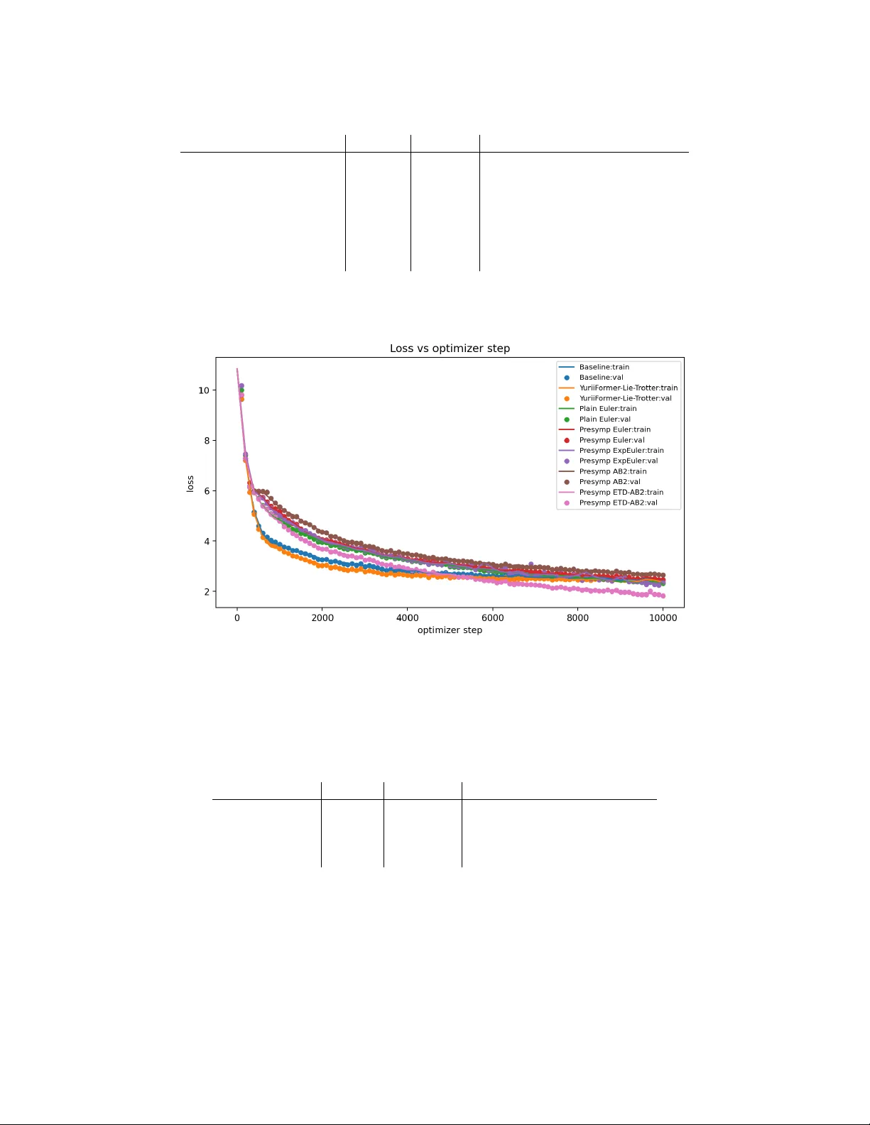
SympF ormer: A ccelerated atten tion blo c ks via Inertial Dynamics on Densit y Manifolds Viktor Stein ∗ , W uc hen Li † , Gabriele Steidl ∗ Marc h 18, 2026 Abstract T ransformers o we muc h of their empirical success in natural language pro cessing to the self-atten tion blo c ks. Recent p erspectives in terpret atten tion blocks as in teracting particle sys- tems, whose mean-field limits corresp ond to gradient flows of interaction energy functionals on probabilit y densit y spaces equipp ed with W asserstein- 2 -type metrics. W e extend this viewpoint b y in tro ducing accelerated atten tion blocks derived from inertial Nesterov-t yp e dynamics on densit y spaces. In our proposed arc hitecture, tokens carry b oth spatial (feature) and velocity v ariables. The time discretization and the approximation of accelerated density dynamics yield Hamiltonian momen tum attention blo c ks, which constitute the prop osed accelerated attention arc hitectures. In particular, for linear self-attention, we sho w that the atten tion blo c ks ap- pro ximate a Stein v ariational gradien t flo w, using a bilinear k ernel, of a p oten tial energy . In this setting, we pro ve that elliptically contoured probability distributions are preserved by the accelerated attention blo cks. W e present implementable particle-based algorithms and demon- strate that the prop osed accelerated atten tion blo c ks con verge faster than the classical atten tion blo c ks while preserving the num b er of oracle calls. Keyw ords: T ransformers; Self-atten tion blo ck; Optimal transp ort; Nesterov’s accelerated gradient metho d; Densit y manifold; Kernel; Hamiltonian dynamics; Symplectic integrators. 1 In tro duction T ransformers [37] underpin mo dern large-scale sequence mo dels and hav e driv en substantial progress in language pro cessing, with large language mo dels, suc h as ChatGPT and Gemini, b ecoming part of ev eryday tools. Despite their empirical success, the mathematical principles underlying the stabilit y , scalabilit y , and training efficiency of transformers remain only partially understo od [7, 13, 14]. The key nov elty of the transformer architecture is the atten tion blo ck, whic h is defined by three linear pro jections of the tok en features: queries, keys, and v alues. Eac h tok en is up dated as a w eighted aggregation of v alue vectors with weigh ts determined by the pairwise similarity b et w een queries and ke ys by a softmax op erator. ∗ Institute of Mathematics, T ec hnische Universität Berlin, Straße des 17. Juni 136, 10623 Berlin, Germany , {stein,steidl}@math.tu-berlin.de , https://tu.berlin/imageanalysis . † Department of Mathematics, Univ ersity of South Carolina, Columbia. 1523 Greene St, Colum bia, SC 29208, USA, wuchen@mailbox.sc.edu . 1 Recen t dev elopments suggest that transformers, and in particular attention blo c ks, can b e in- terpreted as discrete-time in teracting particle dynamics. Eac h la yer up date may b e viewed as a time- and particle-discretization of non-linear evolution equations in probability density spaces ov er high-dimensional feature spaces for tokens. Under suitable choices of attention lay ers, the evolution of tokens resembles gradient descent of an in teraction energy functional. Consequen tly , the proba- bilit y density function of the tokens follows the gradient flow of an energy functional in a probability space equipp ed with a W asserstein-2-t yp e metric, where the mobilit y function is induced by the softmax op erator applied to query , key , and v alue vectors. Gradien t flows in W asserstein spaces ha ve been extensively studied in optimal transp ort theory , including con vergence analysis and numerical sc hemes; for an ov erview, see, e.g. [2, 29, 26]. A classic example is the F okker-Planc k equation [20], which is the gradient flow of the free energy in W asserstein- 2 space. More recent works extend the W asserstein spaces and gradient flows with general mobilit y functions [6, 8], whic h are also within the scop e of dynamical densit y functional theory [36]. How ev er, the analytical and computational prop erties of atten tion-induced mobilities and their asso ciated interaction energies are still under inv estigation. Moreov er, b ey ond the archi- tecture’s gradien t-flow interpolation, training itself corresp onds to an optimization pro cedure ov er the space of probabilit y densities. These observ ations motiv ate a systematic mathematical mo del of transformers based on v ariational principles in probability density spaces. F rom an optimization p erspective, the Nestero v acceleration metho d [24, 25] arises b y introduc- ing momentum into gradient descent. This metho d reduces oscillations and conv erts slow gradient motion into inertial motion, thereby improving the con vergence rate of conv ex optimization in the discrete-time setting from O (1 /k ) to O (1 /k 2 ) . In contin uous time, it corresp onds to a second-order dynamical system related to heavy-ball or damp ed Hamiltonian dynamics [33, 34]. Suc h acceler- ated dynamics hav e recently b een studied on densit y manifolds endow ed with W asserstein- 2 type metrics, including accelerated W asserstein gradient flo ws and accelerated Stein v ariational gradi- en t flows [32, 31]. Existing connections b etw een transformers and interacting particle systems [23] do not y et provide an inertial mec hanism, except for the very recen t work [41]. An acceleration principle arises from the geometry of the probability space go verning tok en evolution. If standard transformers corresp ond to gradient flows on density manifolds, then accelerated transformers may b e constructed from inertial dynamics on density manifolds. This observ ation motiv ates tw o nat- ural questions: What ar e “ac c eler ate d attention blo cks”? Can this ac c eler ate d me chanism impr ove the tr aining pr o c e dur e, at le ast numeric al ly? This work presents our initial ideas for formulating accelerated transformer architectures based on accelerated dynamics on density manifolds. W e apply the fact that transformer lay ers can be in terpreted as particle discretizations of W asserstein-type gradien t flo ws of in teraction energies. W e then deriv e a second-order extension, expressed in terms of momentum and Hamiltonian transformer blo c ks, in which tokens carry b oth feature and velocity v ariables. The resulting dynamics corresp ond to inertial evolution equations in the probabilit y space. W e consider it as an analog of Nesterov’s con tinuous-time acceleration metho ds for constructing accelerated attention blo cks. In the literature, several researc h directions ha ve in vestigated the mathematical prop erties of transformers using optimal transp ort gradient flows. One is Sinkformer [7], which establishes a con- nection b etw een transformers, the Sinkhorn algorithm, and PDEs in the density space. Motiv ated b y [27, 7, 22], a transformer structure has b een studied, which results in the regularized W asser- stein proximal op erator for sampling algorithms [17, 18, 35]. The other direction [14, 12] studies the classical transformer architecture from the p erspective of generalized W asserstein-2 gradient flows. Recen tly , [7] inv estigated transformer PDEs as interacting particle systems. The transformer PDE 2 itself is a gradient flo w with respect to the W asserstein-2 metric with non-linear mobility . This pap er follo ws the second direction by developing accelerated gradient flows and then designing ac- celerated attention blo c ks. More closely to this pap er, w e b ecame aw are of recent work [41], which also addresses a Nesterov-st yle accelerated transformer that preserves the same attention and Mul- tila yer p erceptron (MLP) oracles. How ever, in contrast to our work, the authors of [41] study the “classical” Nesterov acceleration in Euclidean space, which does not consider the damp ed Hamilto- nian dynamics in densit y manifolds. W e included a n umerical comparison with their approac h in this pap er, and sho w the adv antage in terms of the cross-en tropy loss. This pap er is organized as follo ws. In Section 2, w e review Nestero v’s acceleration metho d on Euclidean spaces and in probability density spaces, and geometric integrators for damp ed Hamilto- nian systems. Then, Section 3 recalls the transformer architecture and, in particular, the attention blo c ks from the p ersp ectiv e of a v ariational flow on a probability space. W e deal with linear atten- tion la y ers in Section 4. W e will show that the associated transformer PDE is the Stein gradient flo w of a quadratic p otential energy . This flo w preserves elliptically con toured distributions. W e pro vide a Lagrangian spatial discretization that yields a second-order-in-time inertial in teracting particle system. Section 5 deals with the practically more relev ant softmax self-atten tion. Here, the transformer PDE is a gradient flo w in the softmax-self-atten tion-mobility W asserstein space. W e deriv e the accelerated gradien t flow and pro vide a second-order-in-time inertial interacting particle system. Finally , we demonstrate the p erformance of our accelerated transformer flo ws by numerical examples in Section 6. All pro ofs and deriv ations are provided in App endix A. Implementation details are deferred to Section B. 2 Nestero v’s A cceleration Metho d In this section, w e briefly review Nesterov accelerated gradien t flo ws in Euclidean space and in the space of probability densities equipp ed with the W asserstein- 2 metric or the Stein-W asserstein metric. Nestero v acceleration [24] is a well-kno wn technique for improving the conv ergence rate of gra- dien t descent metho ds. Consider the optimization problem: min x ∈ R d F ( x ) , (1) where F ∈ C 1 ( R d ; R ) is an objective function. The gradient descent sequence starting at x 0 ∈ R d is x ( k +1) = x ( k ) − τ ∇ F ( x ( k ) ) , x (0) = x 0 , where k ∈ N is the iteration step and τ > 0 is a step size. Nesterov’s accelerated gradient descent is obtained by choosing an extrap olation co efficien t, as in the left part of (2). Substituting t = k √ τ and letting τ → 0 , Nestero v’s metho d can b e in terpreted through a contin uous-time dynamical system [33]:        x ( k +1) = y ( k ) − τ ∇ F ( y ( k ) ) , y ( k +1) = x ( k +1) + (1 − 3 k +3 )( x ( k +1) − x ( k ) ) , x (0) = x 0 , y (0) = x 0 .    ¨ x ( t ) + 3 t ˙ x ( t ) + ∇ F ( x ( t )) = 0 , x (0) = x 0 , ˙ x (0) = 0 . (2) 3 F or a conv ex function F and any step size τ ∈ (0 , 1 L ) , where L is the Lipsc hitz constant of ∇ F , the discrete sc heme exhibits a conv ergence rate F ( x ( k ) ) − F ∗ ≤ O ( ∥ x 0 − x ∗ ∥ τ k 2 ) , where x ∗ is a minimizer of F and F ∗ = F ( x ∗ ) . This rate is optimal among all methods having only information ab out the gradient of F at consecutive iterates [25]. F or the con tinuous dynamics, w e ha ve similarly F ( x ( t )) − F ∗ ≤ O ( ∥ x 0 − x ∗ ∥ t 2 ) . In tro ducing the momentum v ariable p t , the second-order ODE (2) can also b e rewritten as the first-order system ˙ x t = p t , ˙ p t = − α t p t − ∇ F ( x t ) , x t | t =0 = x 0 , p 0 = 0 , (3) where α t : = 3 t . Interestingly , it w as observed in [34] that with the Hamiltonian function and its deriv atives H ( x, p ) = 1 2 ∥ p ∥ 2 + F ( x ) , ∇ p H ( x, p ) = p, ∇ x H ( x, p ) = ∇ F ( x ) , the first-order system (3) b ecomes a damp ed Hamiltonian flow  ˙ x t ˙ p t  +  0 α t p t  −  0 I d − I d 0   ∇ x H ( x t , p t ) ∇ p H ( x t , p t )  = 0 , x t | t =0 = x 0 , p 0 = 0 . (4) In [38], the damp ed Hamiltonian flow (4) was directly generalized for accelerating gradien t flo ws on the probability density space. Let Ω = R d and P (Ω) : = { ρ ∈ C ∞ > 0 (Ω) : Z Ω ρ ( x ) d x = 1 } . F or densities ρ ∈ P (Ω) , w e denote the tangent space at ρ by T ρ P (Ω) = { σ ∈ C ∞ (Ω) : Z Ω σ d x = 0 } , and its cotangent space by T ∗ ρ P (Ω) ∼ = C ∞ (Ω) / R . F or an y densit y function ρ ∈ P (Ω) , a metric tensor is an inv ertible mapping op erator G ρ : T ρ P (Ω) → T ∗ ρ P (Ω) , whic h defines a metric on T ρ (Ω) b y ⟨ σ 1 , σ 2 ⟩ ρ : = Z Ω σ 1 G ρ [ σ 2 ] d x = Z Ω Φ 1 G − 1 ρ [Φ 2 ] d x, where σ i = G − 1 ρ Φ i , i = 1 , 2 with σ i ∈ T ρ P (Ω) and Φ i ∈ T ∗ ρ P (Ω) . In this pap er, we are mainly in terested in the following metrics: W asserstein : ( G W ρ ) − 1 Φ : = −∇ · ( ρ ∇ Φ) , Stein : ( G S ρ ) − 1 Φ : = −∇ ·  ρ Z Ω k ( · , y ) ∇ Φ( y ) ρ ( y ) d y  , (5) where k : Ω × Ω → R is a symmetric, in tegrally strictly p ositiv e definite kernel with R Ω k ( x, x ) d x < ∞ . Then, w e study the minimization problem of a functional F : P (Ω) → R in the probability densit y space: min ρ ∈P (Ω) F ( ρ ) . The gradient flow of energy functional F ( ρ ) in the probabilit y density space ( P (Ω) , G ) satisfies ∂ t ρ t = − G − 1 ρ t h δ F ( ρ t ) δ ρ t i . (6) 4 Here, δ F ( ρ t ) δ ρ t ∈ T ∗ ρ P (Ω) denotes the L 2 first v ariation of functional F ( ρ ) at the density ρ defined by Z Ω δ F ( ρ t ) δ ρ t φ d x = lim ε → 0 1 ε ( F ( ρ + ϵφ ) − F ( ρ )) , for all φ ∈ C ∞ (Ω) with mass zero for which ρ + ϵφ ∈ P (Ω) . Then the acceleration dynamics (4) in ( P (Ω) , G ) , suggested in [38], satisfies ∂ t  ρ t Φ t  +  0 α t Φ t  −  0 I − I 0  δ δ ρ t H ( ρ t , Φ t ) δ δ Φ t H ( ρ t , Φ t ) ! = 0 , ρ t | t =0 = ρ 0 , Φ 0 = 0 , (7) where ρ 0 ∈ P (Ω) is a given initial density function, I denotes the identit y op erator on T ∗ ρ P (Ω) , and the Hamiltonian functional H : P (Ω) × T ∗ ρ P (Ω) → R satisfies H ( ρ t , Φ t ) : = 1 2 Z Ω Φ t G − 1 ρ t [Φ t ] d x + F ( ρ t ) . (8) Indeed, this accelerated gradient method relies on tw o ingredients, namely the functional F and the metric tensor G ρ . The system (7) can b e rewritten as    ∂ t ρ t − G − 1 ρ t [Φ t ] = 0 , ρ t | t =0 = ρ 0 , ∂ t Φ t + α t Φ t + 1 2 δ δ ρ t  R Ω Φ t G − 1 ρ t [Φ t ] d x  + δ F δ ρ t = 0 , Φ 0 = 0 . (9) F or example, the accelerated gradient flow (9) in these density manifolds b ecomes W asserstein:    ∂ t ρ t + ∇ · ( ρ t ∇ Φ t ) = 0 , ρ t | t =0 = ρ 0 , ∂ t Φ t + α t Φ t + 1 2 ∥∇ Φ t ∥ 2 2 + δ F ( ρ t ) δ ρ t = 0 , Φ 0 = 0 . (10) Stein:    ∂ t ρ t + ∇ ·  ρ t ( x ) R Ω k ( x, y ) ρ t ( y ) ∇ Φ t ( y ) d y  = 0 , ρ t | t =0 = ρ 0 , ∂ t Φ t + α t Φ t + R Ω ∇ Φ t ( x ) T ∇ Φ t ( y ) k ( x, y ) ρ t ( x ) d x + δ F ( ρ t ) δ ρ t = 0 , Φ 0 = 0 . (11) This formalism is only rigorous on compact manifolds; w e treat the case of Ω = R d only formally . A fruitful av enue for future research is to mo del lay er normalization as a projection onto the sphere, thereb y placing the dynamics on a compact manifold. W e will discretize certain accelerated gradient flo ws by appro ximating the density ρ t b y the empirical measure 1 N P N j =1 δ X i ( t ) and setting Y i ( t ) : = ∇ Φ t ( X i ( t )) , yielding a finite-dimensional linearly damped Hamiltonian system in Euclidean space (4). Later, w e will leverage that (4) can b e rewritten as the undamp e d Hamiltonian system ( ˙ x ( t ) = ∂ P ˜ H  t, x ( t ) , P ( t )  , x (0) = x 0 , ˙ P ( t ) = − ∂ q ˜ H  t, x ( t ) , P ( t )  , P (0) = 0 , (12) with the time-dep endent Hamiltonian ˜ H ( t, q , P ) : = e η ( t ) H ( q, e − η ( t ) P ) , t ≥ t 0 , using the chan ge of v ariables P = e η ( t ) p, (13) see, e.g., [10, App. B] and also [39]. 5 Time Discretizations of Linearly Damp ed Hamiltonian Systems Let η : [ t 0 , ∞ ) → R , t 7→ R t t 0 α ( s ) d s b e a w ell-defined antideriv ative for α , for some fixed t 0 ≥ 0 . F or example, if α ( t ) ≡ µ > 0 , then we can pick t 0 = 0 and then η ( t ) = µt , whereas if α ( t ) = 3 t , then we will choose t 0 > 0 and obtain η ( t ) = 3 ln ( t/t 0 ) . F urther, let h k > 0 denote the step sizes. W e use the time grid t k +1 : = t k + h k for k ∈ N for some t 0 ≥ 0 and denote by σ k : = exp  − R t k +1 t k α ( s ) d s  the discrete damping co efficien t for k ∈ N , whic h mimics the contin uous-time dissipation [1]. F or common damping schedules α , the damping co efficien t is av ailable in closed form. Explicit Euler metho d The most simple time discretization of (4) is a plain explicit forwar d Euler discretization with step size τ > 0 , which do es not take any geometry into account. Its k -th iteration is ( x ( k +1) = x ( k ) + h k ∇ p H ( x ( k ) , p ( k ) ) , p ( k +1) = α k p ( k ) − h k ∇ x H ( x ( k ) , p ( k ) ) , (14) where α k = k − 1 k +2 or α k is constant. This Nesterov-st yle discretization is not conformally symplectic [10, 11]. Conformally symplectic Euler metho d A geometric approac h [15, 4] is to split the vector field ( ∂ p H , − αp − ∂ q H ) driving the evolution (4) into its conserv ative part ( ∂ p H , − ∂ q H ) and the dissipativ e part (0 , − αp ) . W e apply a Lie-T rotter split: integrate the dissipative part exactly and use a symplectic integrator for the conserv ative part. This is known as the c onformal ly symple ctic Euler or “kick then damp” scheme , which reads ( p ( k +1) = σ k  p ( k ) − h k ∇ x H ( x ( k ) , p ( k ) )  , x ( k +1) = x ( k ) + h k ∇ p H ( x ( k ) , p ( k +1) ) . (15) Exp onen tial Euler metho d F or a simple Hamiltonian, whose kinetic energy term is just 1 2 ∥ p ∥ 2 , the dynamics (4) can b e written as ˙ p + αp − ∇ x H ( x, p ) = 0 . Hence, w e can use the exp onential Euler metho d [19] applied to this simplified evolution to approximately discretize (4) for general Hamiltonians. The exp onen tial Euler up date for fixed step size h k = h > 0 reads as follows: ( p ( k +1) = σ k p ( k ) − h R h 0 exp  − R h s α ( z ) d z  d s ∇ x H ( x ( k ) , p ( k ) ) , x ( k +1) = x ( k ) + h ∇ p H ( x ( k ) , p ( k ) ) . (16) F or α ( s ) = r s , the weigh t in front of ∇ x H in the first up date equation b ecomes h r +1 and for α ( s ) = m , it b ecomes 1 − e − mh m . F or the log-linear damping α ( s ) = r s + m , it can b e expressed in terms of the confluen t hypergeometric function 1 F 1 . F or the accelerated transformer arc hitecture presented in Sections 4 and 5, we need time dis- cretizations that require a small num b er of function ev aluations (also called oracle calls). First-order time-discretizations ev aluate the function only once p er iteration. Multi-step metho ds can achiev e higher orders of accuracy than first-order metho ds b y reusing function v alues from previous iter- ations, thereby preserving the oracle budget. In contrast, higher-order single-step metho ds like R unge-Kutta-4 need four oracle calls p er step. 6 A dams-Bashforth (AB-2) metho d The tw o-step Adams-Bashforth (AB-2) [3] is an explicit linear multistep metho d of or der two – the b est order ac hiev able by an explicit tw o-step multistep metho d [16, Chp. 3]. W e can write (4) abstractly as an ODE of the form y ′ ( t ) = f ( t, y ( t )) , where y = ( x, p ) . The AB-2 metho d then is y ( k +1) = y ( k ) + h k  2 h k − 1 + h k 2 h k − 1 f ( t ( k ) , y ( k ) ) − h k 2 h k − 1 f ( t ( k − 1) , y ( k − 1) )  . (17) Here h k > 0 is a stepsize. T o obtain the v alue y (1) from the giv en initial v alue y (0) , we p erform an explicit Euler step: y (1) = y (0) + h 0 f ( t 0 , y (0) ) . 3 T ransformers In this section, we briefly review transformers from the viewp oin t of PDEs on the space of probabilit y densities; for details, see, e.g. [7, 14]. T ransformers mo dify tok en configurations ( X 1 , . . . , X N ) ∈ ( R d ) N using t wo essential compo- nen ts, namely self-atten tion la yers, whic h com bine information across tokens, and MLP la yers, whic h p erform indep enden t non-linear transforms on each tok en. Let Q, K ∈ R m × d and V ∈ R d × d , m ≤ d , b e query , key , and v alue matrices, which usually differ in each lay er of the transformer, and set A : = K T Q ∈ R d × d . W e assume that A is a symmetric matrix. In this pap er, we are interested in functions κ = κ A : R d × R d → R in one of the following forms: κ ( X i , X j ) =      exp ( ( X j ) T AX i ) P N ℓ =1 exp(( X ℓ ) T AX i ) = softmax j  ( X T ℓ AX i ) N ℓ =1  softmax self-attention , ( X j ) T AX i linear self-attention . (18) Recall that the softmax function is defined b y softmax ( w ) : =  exp( w i ) / P d j =1 exp( w j )  d i =1 , for w ∈ R d . Then, one lay er of a transformer consists of the subla yers: Self-atten tion la yer : X ( k +1) i = X ( k ) i + h N X j =1 κ ( X ( k ) i , X ( k ) j ) V X ( k ) j . (19) MLP la y er : X ( k +1) i = X ( k ) i + hW σ ( ˜ W X ( k ) i + b ) , (20) where we denote the input tok ens as ( X 0 1 , · · · , X 0 N ) , h > 0 is a step size, k ∈ N is the depth of the la yer, W, ˜ W ∈ R d × d are the w eight matrices, and the bias vector b ∈ R d differs in general in each la yer, and σ : R → R is a non-linear function applied comp onen twise. This description assumes that the matrices Q , K , and V are the same in each lay er (“w eight sharing”), whic h is the case for some transformer arc hitectures, such as ALBER T [21]. W e next presen t an ODE system only for the attention lay er describ ed ab ov e. As the step size h → 0 , w e obtain the following ODE system. Giv en input tok ens X (0) = ( X 1 (0) , . . . , X N (0)) ∈ ( R d ) N , their evolution through an attention lay er can b e mo deled as a dynamical system ˙ X i ( t ) = Γ X ( t ) ( X i ( t )) , 1 ≤ i ≤ N , (21) 7 where Γ X : R d → R d denotes the atten tion vector field determined b y the query , key , and v alue matrices Q , K , V for the current total tok ens X ( t ) . In the case of softmax self-atten tion, the v ector field takes the form: Γ X ( x ) : = N X j =1 exp  Qx · K X j  P N ℓ =1 exp  Qx · K X ℓ  V X j , for x ∈ R d . Eac h tok en in (21) evolv es as a similarit y-weigh ted av erage of the v alue v ectors, whic h follo ws a non-linear interacting particle system. By [7, 14], see also [5, 13, 28, 40], the mean-field limit of the in teracting particle system (21) with only self-attention blo c ks can b e expressed for Ω = R d as ∂ t ρ t = −∇ · ( ρ t Γ ρ t ) , t > 0 , (22) where the velocit y field is a probabilit y densit y dep enden t vector function satisfying: Γ ρ : R d → R d , x 7→ Z V y κ ρ ( x, y ) ρ ( y ) d y . In this pap er, we are in terested in the following tw o atten tion lay ers: κ ρ ( x, y ) : =    exp( y T Ax ) R exp( z T Ax ) ρ ( z ) d z softmax self-attention , y T Ax, linear self-attention . As sho wn for accelerating the gradient flow (6) in the previous section, we prop ose to accelerate the flo w (22). W e start with the simple linear self-attention in Section 4 and then consider the softmax self-atten tion in Section 5. 4 A ccelerated T ransformers with Linear A tten tion In this section, for the linear self-atten tion, we sho w that the asso ciated transformer PDE is the Stein v ariational gradien t flo w of a quadratic p oten tial energy . W e pro ve that this flo w preserv es elliptically contoured distributions and pro vide a spatial discretization that yields a second-order- in-time inertial in teracting particle system. In this section, w e assume that A is symmetric and p ositiv e definite. 4.1 A ccelerated Flo w F or the linear attention, the transformer PDE (22) reads as ∂ t ρ t = −∇ ·  ρ t ( x ) Z y T Ax V y ρ t ( y ) d y  . (23) Assume that V is symmetric. F or the p oten tial energy F lin : P ( R d ) → R ∪{±∞} given by F lin ( ρ ) : = − 1 2 Z y T V y ρ ( y ) d y , 8 w e hav e that h δ F lin ( ρ ) δ ρ i ( y ) = − 1 2 y T V y , ∇ y h δ F lin ( ρ ) δ ρ i = − V y . Th us, defining the inv erse metric tensor by ( G lin ρ ) − 1 [Φ] : = −∇ ·  ρ ( x ) Z y T Ax ∇ Φ( y ) ρ ( y ) d y  , w e conclude that ∂ t ρ t = − ( G lin ρ t ) − 1 " δ F lin ( ρ t ) δ ρ t # . This transformer PDE is exactly the Stein v ariational gradient flow (5) with resp ect to the energy functional F lin with kernel k ( x, y ) : = y T Ax . F or the linear self-attention, the accelerated gradien t flo w in (9) can b e specified as in the follo wing prop osition. The pro of is given in App endix A. Prop osition 4.1 (A ccelerated linear atten tion PDE) . The ac c eler ate d line ar self-attention tr ans- former flow in (9) satisfies ( ∂ t ρ t ( x ) + ∇ ·  ρ t ( x ) R y T Ax ∇ Φ t ( y ) ρ t ( y ) d y  = 0 , ρ t | t =0 = ρ 0 ∂ t Φ t ( x ) + α t Φ t ( x ) + R ⟨∇ Φ t ( x ) , ∇ Φ t ( y ) ⟩ y T Axρ t ( y ) d y − 1 2 x T V x = 0 , Φ 0 = 0 . (24) Her e, ( α t ) t> 0 ar e non-ne gative damping p ar ameters. 4.2 Preserv ation of Elliptically Con toured Distributions W e sho w that if the initial density ρ 0 is elliptically contoured, e.g., a Gaussian distribution, then the solution ρ t of (24) will remain so for all times. A probabilit y densit y ρ on R d is called el liptic al ly c ontour e d [30, Sec. 5] [9, Sec. 3]. W e write ρ = E ( m, Σ , g ) , if ρ can b e expressed as det(Σ) − 1 2 g  ( · − m ) T Σ − 1 ( · − m )  , for some m ∈ R d , Σ ∈ Sym + ( R ; d ) and some smo oth, integrable function g : [0 , ∞ ) → (0 , ∞ ) fulfilling i) normalization: R ∞ 0 r d 2 − 1 g ( r ) d r = Γ ( d 2 ) π d 2 ; ii) finite exp ectation: R ∞ 0 r d − 1 2 g ( r ) d r < ∞ ; iii) finite v ariance: R ∞ 0 r d 2 g ( r ) d r < ∞ . W e study elliptically contoured distributions b ecause this family is inv ariant under the pushfor- w ard mapping function b y affine linear functions: given the affine linear map f ( x ) : = Ax + b for a matrix A ∈ R d × d and a v ector b ∈ R d , we hav e that ρ = E ( m, Σ , g ) implies that the pushforward densit y of ρ by f is elliptically contoured, namely E ( Am + b, A Σ A T , g ) , see [9, p. 279]. 9 Example 4.2 (Elliptically contoured distributions) . F or g ( x ) = (2 π ) − d 2 e − 1 2 x , we obtain Gaussian distributions, and for g ( x ) = Γ ( v + d 2 ) Γ ( v 2 ) ( v π ) − d 2  1 + 1 v x  − v + d 2 , we get the multivariate Student-t distri- butions with v > 2 de gr e es of fr e e dom. Ther e ar e also other less-known examples, such as lo gistic distributions, even p ower-exp onential distributions, and gener alize d hyp erb olic distributions, se e [30, Se c. 6]. The exp ectation v alue and the v ariance of an elliptic distribution are, resp ectively E X ∼ E ( m, Σ ,g ) [ X ] = m, V X ∼ E ( m, Σ ,g ) [ X ] = κ g Σ , where κ g : = 1 d Z ∥ y ∥ 2 g ( ∥ y ∥ 2 ) d y . F or Gaussian distributions, w e hav e κ g = 1 and for the Student- t distribution with v degrees of freedom κ g = v v − 2 . By the following prop osition, whose pro of is given in App endix A, the accelerated linear trans- former PDE (24) preserves elliptically contoured distributions. Prop osition 4.3 (Preserv ation of elliptically contoured distributions) . L et ( ρ t , Φ t ) t ≥ 0 satisfy (24) and ρ 0 = E ( m, Σ , g ) . Then it holds ρ t = E ( m t , Σ t , g ) and Φ t ( x ) = 1 2 x T P t x, with m t and Σ t , P t ∈ Sym ( R ; d ) determine d by ( ˙ m t = C t m t , m t | t =0 = m 0 , ˙ Σ t = Σ t C T t + C t Σ t , Σ t | t =0 = Σ 0 , (25) wher e C t : = P t ( κ g Σ t + m t m T t ) A and ( ˙ P t = − α t P t − ( C T t P t + P t C t ) + V , t > 0 , P 0 = 0 . (26) If the initial density ρ 0 has zero mean, then we obtain the follo wing more simple evolution of ρ t . Corollary 4.4 (Preserv ation of centered elliptically contoured distributions) . L et ( ρ t , Φ t ) t ≥ 0 satisfy (24) and ρ 0 = E (0 , Σ , g ) . Then, ρ t = E (0 , Σ t , g ) and Φ t ( x ) = 1 2 x T P t x, with Σ t , P t ∈ Sym ( R ; d ) determine d by ˙ Σ t = κ g (Σ t A Σ t P t + P t Σ t A Σ t ) , and ( ˙ P t = − α t P t − κ g ( A Σ t P 2 t + P 2 t Σ t A ) + V , t > 0 , P 0 = 0 . (27) 10 4.3 A ccelerated Linear Atten tion Dynamics W e now discretize (24) in space. F or t > 0 , w e appro ximate the densit y ρ t b y the empirical measure 1 N P N j =1 δ X i ( t ) . In App endix A, we provide the follo wing discretization result. Prop osition 4.5. The deterministic inter acting p article system asso ciate d to (24) is ( ˙ X i ( t ) = 1 N P N j =1 Y j ( t ) X j ( t ) T AX i ( t ) , X i (0) = X i, 0 , ˙ Y i ( t ) = − α t Y i ( t ) − 1 N P N j =1 ⟨ Y i ( t ) , Y j ( t ) ⟩ AX j ( t ) + V X i ( t ) , Y i (0) = 0 , wher e Y i ( t ) = ∇ Φ t ( X i ( t )) . In the matrix form, the ab ove system satisfies ( ˙ X ( t ) = 1 N X ( t ) A X ( t ) T Y ( t ) , X (0) = X 0 , ˙ Y ( t ) = − α ( t ) Y ( t ) − 1 N Y ( t ) Y ( t ) T X ( t ) A + X ( t ) V , Y (0) = 0 . (28) The explicit Euler discretization (14) with step sizes ( h k ) k ∈ N of (28) is ( X ( k +1) = X ( k ) + h k N X ( k ) A ( X ( k ) ) T Y ( k ) , X (0) = X 0 , Y ( k +1) = α k Y ( k ) − h k N Y ( k )  Y ( k )  T X ( k ) A + X ( k ) V , Y (0) = 0 . 5 A ccelerated T ransformers with Softmax atten tion In this section, we present the main result of this pap er. F or the softmax self-attention, we briefly review that the transformer PDE is a gradien t flow in a softmax self-attention mobility W asserstein sp ac e ( P , G SM ρ ) [14]. W e then deriv e the accelerated gradient flow in ( P , G SM ρ ) , for which we provide first- and second-order-in-time inertial interacting particle systems for the softmax self-atten tion la yer. 5.1 A ccelerated Flo w F or the softmax self-attention, the transformer PDE (22) reads as ∂ t ρ t = −∇ ·  ρ t ( x ) Z V y exp( y T Ax ) R exp( z T Ax ) ρ t ( z ) d z ρ t ( y ) d y  . F or the energy F SM : P ( R d ) → R ∪{±∞} given by F SM ( ρ ) : = − 1 2 Z Z exp( y T Ax ) ρ ( x ) ρ ( y ) d x d y , (29) w e hav e that h δ F SM ( ρ ) δ ρ i = − Z exp  y T Ax  ρ ( y ) d y , (30) ∇ x h δ F SM ( ρ ) δ ρ i = − Z exp  y T Ax  Ay ρ ( y ) d y . (31) 11 Th us, defining the inv erse metric tensor by ( G SM ρ ) − 1 [Φ] : = −∇ ·  ρ V A − 1 ∇ x Φ R exp ( z T Ax ) ρ ( z ) d z  . (32) W e observ e that the transformer PDE satisfies ∂ t ρ t = − ( G SM ρ t ) − 1 " δ F SM ( ρ t ) δ ρ t # . Assume that B : = V A − 1 , is symmetric and p ositiv e definite. Then the transformer PDE resembles the W asserstein-2 type gradien t flow with a nonlinear mobility matrix function χ : P (Ω) → C ∞ (Ω) d × d : ∂ t ρ t = ∇ ·  χ ( ρ t ) ∇ h δ F SM ( ρ t ) δ ρ t i , χ ( ρ )( x ) : = ρ ( x ) R exp ( z T Ax ) ρ ( z ) d z V A − 1 . F urthermore, we introduce the notation ∥ v ∥ 2 B : = ⟨ v , B v ⟩ , v ∈ R d . The following proposition sp ecifies the accelerated gradient flow in (9) for the softmax self-attention la yer. The pro of is provided in A. Prop osition 5.1 (Accelerated softmax attention PDE) . The ac c eler ate d softmax attention flow in (9) satisfies                        ∂ t ρ t ( x ) + ∇ ·  ρ t ( x ) V A − 1 ∇ Φ t ( x ) R exp ( z T Ax ) ρ t ( z ) d z  = 0 , ρ t | t =0 = ρ 0 , ∂ t Φ t ( x ) + α t Φ t ( x ) + 1 2 ∥∇ Φ t ( x ) ∥ 2 B R exp ( z T Ax ) ρ t ( z ) d z − 1 2 Z exp  y T Ax  ∥∇ Φ t ( y ) ∥ 2 B  R exp ( z T Ay ) ρ t ( z ) d z  2 + 2 ! ρ t ( y ) d y = 0 , Φ 0 = 0 . (33) 5.2 A ccelerated Softmax Atten tion Dynamics F or t > 0 , we appro ximate the density ρ t b y the empirical measure 1 N P N j =1 δ X i ( t ) . In App endix A, w e prov e the following discretization result. Prop osition 5.2. The deterministic inter acting p article system asso ciate d to (33) is for i = 1 , . . . , N given by              ˙ X i ( t ) = N B Y i ( t ) P N j =1 M i,j ( t ) , ˙ Y i ( t ) = − α t Y i ( t ) + N 2 A N X j =1 X j ( t ) M i,j ( t )    ∥ Y i ( t ) ∥ 2 B  P N k =1 M i,k ( t )  2 + ∥ Y j ( t ) ∥ 2 B  P N k =1 M j,k ( t )  2 + 2    , wher e Y i ( t ) : = ∇ Φ t ( X i ( t )) and M i,j ( t ) : = exp  X i ( t ) T AX j ( t )  . 12 Remark 5.3. L et X ( t ) ∈ R N × d have the r ows X i ( t ) ∈ R d , and Y ( t ) b e define d analo gously. F ur- ther, set M ( t ) : = ( M i,j ( t )) N i,j =1 , R : = diag  ( Y ⊙ Y B T ) 1 d ⊘  ( M 1 ) ⊙ ( M 1 )  , and let { R , M } : = RM + MR denote the anti-c ommutator. F urther, denote elementwise multiplic ation and division by ⊙ and ⊘ , r esp e ctively. Then, we c an write the ab ove system c omp actly as fol lows: ( ˙ X ( t ) = N diag ( M ( t ) 1 ) − 1 Y ( t ) B T , ˙ Y ( t ) = − α t Y ( t ) + N 2  { R ( t ) , M ( t ) } + 2 M ( t )  X ( t ) A. (34) Consider the c onservative p art of (34) , i.e., (34) without the term α ( t ) Y ( t ) . A Hamiltonian for the system is H SM : R N × d × R N × d → R , ( X , Y ) 7→ N 2 tr(diag( M 1 ) − 1 Y B T Y T ) − N 2 1 T M 1 . (35) The se c ond summand of H SM is a c onstant multiple of the p article appr oximation of the p oten- tial ener gy (29) . This Hamiltonian is non-sep ar able: its first summand dep ends on Y and on X simultane ously, r esulting in a major differ enc e b etwe en our work and the scheme fr om [41]. W e no w apply the time discretizations outlined in Section 2 to the accelerated transformer with softmax self-atten tion (34). W e view the discretized time up date as the accelerated softmax atten tion lay er. Example 5.4. The time-dep endent Hamiltonian b elonging to the c onservative softmax-Hamiltonian (35) for (34) is ˜ H SM : R × R N × d × R N × d → R , ( t, Q , P ) 7→ N 2  e − η ( t ) tr  diag( M ( Q ) 1 ) − 1 P B T P T  − e η ( t ) 1 T M ( Q ) 1  . (36) Example 5.5. F or softmax self-attention, the plain explicit Euler metho d (14) b e c omes          M ( k ) = exp  X ( k ) A ( X ( k ) ) T  , X ( k +1) = X ( k ) + τ N diag ( M ( k ) 1 ) − 1 Y ( k ) B T , R ( k ) = diag  Y ( k ) ⊙ Y ( k ) B ) 1 d ⊘  ( M ( k ) 1 ) ⊙ ( M ( k ) 1 )  , Y ( k +1) = − α k Y ( k ) + τ 2 N  { R ( k ) , M ( k ) } + 2 M ( k )  X ( k +1) A. F urther, the exp onential Euler metho d (16) satisfies            M ( k ) = exp  X ( k ) A ( X ( k ) ) T  , X ( k +1) = X ( k ) + hN diag( M ( k ) 1 ) − 1 Y ( k ) B T , R ( k ) = diag  Y ( k ) ⊙ Y ( k ) B ) 1 d ⊘  ( M ( k ) 1 ) ⊙ ( M ( k ) 1 )  , Y ( k +1) = σ k Y ( k ) + h R h 0 exp  − R h s α ( z ) d z  d s N 2  { R ( k ) , M ( k ) } + 2 M ( k )  X ( k ) A. 6 Numerical Results Finally , we demonstrate the numerical performance of our method 1 . The goal of the deco der- only causal nanoGTP-style transformer is to predict the next token. All mo dels end with a final 1 The co de repro ducing the exp erimen ts is av ailable on GitHub: https://github.com/ViktorAJStein/SympFormer . 13 x ℓ y ℓ ¯ x ℓ LN µ att ℓ Attn ℓ + + LN Y x ℓ + 1 2 y ℓ + 1 2 ζ 1 ,ℓ h X ℓ F ℓ h Y ℓ ζ 2 ,ℓ G ℓ ˜ x ℓ LN m MLP ,ℓ MLP ℓ + LN Y y ℓ +1 + x ℓ +1 β MLP ,ℓ γ MLP ,ℓ · d ℓ Figure 1: The accelerated atten tion blo c k follow ed by an accelerated MLP blo c k as described in Algorithm 1. La yerNorm and a linear head, and eac h lay er learns the matrices Q , K , and V . While the theory ab o v e models only single-head self-attention, in our implementation of the accelerated softmax- atten tion, the score matrices are av eraged across attention heads b efore exp onen tiation. T o ev aluate p erformance, w e use a cross-entrop y loss. W e observ e that the oracle-preserving SympF ormer outperforms the baseline and the Y uri- iformer architecture, achieving low er v alidation loss at higher wall-time costs for the same num b er of iterations. 6.1 The SympF ormer arc hitecture In the follo wing, we explain the differences b et w een the mathematical formalism introduced ab o ve and the implemen tation. The precise implemen tation details are deferred to Section B. Simplified time discretization Let us denote the right-hand sides of the tw o up date equations in (34) resp. (28) b y F ( X , Y ) and G ( X , Y ) , resp ectiv ely , ignoring the damping term α ( t ) Y ( t ) . In terms of compute, the b ottlenec k of the transformer architecture is ev aluating the self-attention k ernel κ from (18). T o limit the num b er of computations of κ , the SympF ormer uses a simultane ous forw ard Euler up date on b oth X and Y instead of the conformally symplectic Euler sc heme (15), in which the momentum is up dated first, and then the p osition up date uses the new momen tum. T o construct a learnable but principled damping sc hedule, we c ho ose the log-linear damping sc hedule α ( t ) = r t + m [10] for p er-la yer learnable parameters r, m > 0 . Heuristically , this ch oice of damping schedule ensures that the damping decreases ov er time, as in the usual Nesterov sc heme, and also sets a “damping flo or” m to preve nt the damping from b ecoming to o small at later times. In tuitively , for large v alues of t > 0 , the particles should b e in a region where the ob jectives F SM resp. F lin is strongly conv ex, so an approximately constant damping is the correct schedule. W e also learn separate step sizes h k,X and h k,Y for the p osition and momen tum up dates, re- sp ectiv ely , giving the optimizer indep endent control ov er b oth. In the implementation, eac h lay er carries its own attention-step parameters and its own damping sc hedule. Hence, the MLP substep reuses the attention momen tum stream as its look-ahead velocity . W e summarize the architecture in Algorithm 1 and visualize it in Figure 1. 6.2 Comparisons on the Tin yStories data set Both for softmax atten tion and for linear attention, we compare the v anilla transformer architecture (“Baseline”) and the Lie-T rotter Nesterov v ariant of the Y uriiformer architecture [41] with a plain Euler forward discretization (“Plain Euler”), the presymplectic Euler metho d (“Presymp Euler”), 14 Algorithm 1: F orward pass through the SympF ormer – an accelerated transformer. Input: Batch size B ∈ N , token indices idx ∈ { 0 , . . . , V − 1 } B × N , initial time t 0 L blo c ks, each with learned scalar parameters h X ℓ , h Y ℓ > 0 (p osition/momen tum step sizes), MLP scalars m MLP ,ℓ , β MLP ,ℓ ∈ (0 , 1) , γ MLP ,ℓ > 0 learned damping co efficien ts c log , c lin > 0 with η ( t ) = c log ln t + c lin t , which are all used to build the co efficien ts ζ 1 ,ℓ , ζ 2 ,ℓ , defined in table 4, dep ending on the time discretization. Output: Logits ∈ R B × N × V . 1 x ← T okEmb(idx) + P osEmb(pos) // token features 2 y ← 0 // attention momentum 3 for ℓ = 0 , 1 , . . . , L − 1 do 4 ev aluate oracles F and G (right hand side in (34) or (28)) // Accelerated attention step 5 6 α ℓ ← c log /t ℓ + c lin // instantaneous damping rate ˙ η ( t ℓ ) 7 8 y ← ζ 1 ,ℓ y + h Y ℓ ζ 2 ,ℓ G // forward step on y 9 10 x ℓ + 1 2 ← x + h X ℓ F // forward step on x 11 12 y ℓ + 1 2 ← LN Y ( y ) // momentum LayerNorm 13 // Accelerated MLP step 14 ˜ x ℓ ← x ℓ + 1 2 + m MLP ,ℓ y ℓ + 1 2 15 d ℓ ← MLP ℓ (LN( ˜ x ℓ )) 16 y ← LN V  β MLP ,ℓ y ℓ + 1 2 + γ MLP ,ℓ d ℓ  17 x ← x ℓ + 1 2 + y 18 t ← t + h X ℓ 19 logits ← LN f ( x ) W ⊤ lm // final layer norm and linear head 20 return logits the presymplectic exp onential Euler (“Presymp ExpEuler”), and the AB-2 scheme (17) applied to (4) (“Presymp AB2”) and to (12) (“Presymp ETD-AB2”). W e rep ort numerical results on the TinyStories data set, which contains the text from o ver 2000 short stories in T able 1. The exact configurations (num b er of lay ers, num b er of heads, embedding dimension, etc.) are listed in Section B. 15 mo del last ( ↓ ) b est ( ↓ ) wall clo c k time (seconds) ( ↓ ) Baseline 2.4687 2.4473 2409.4 Y uriiF ormer-Lie-T rotter 2.4041 2.3872 2835.2 Plain Euler 2.3247 2.3234 5036.1 Presymp Euler 2.4728 2.4592 4979.0 Presymp ExpEuler 2.3579 2.2523 5623.4 Presymp AB2 2.6653 2.6546 5249.4 Presymp ETD-AB2 1.8386 1.8386 5798.2 T able 1: V alidation loss on the tinystories data set after 10000 optimization steps. Figure 2: V alidation loss (circles) and training loss (lines) on the tinystories data set after 10000 optimization steps, illustrating the results from T able 1. Lastly , w e also rep ort results for the SympF ormer with linear attention in T ables 2 and 3. Again, the exact configurations (n umber of lay ers, num b er of heads, embedding dimension, etc.) are listed in Section B. mo del last ( ↓ ) b est ( ↓ ) w all clo c k time (seconds) ( ↓ ) Baseline 3.0830 2.961427 486.7 Y uriiF ormer 2.8783 2.765975 749.6 plain Euler 3.0399 2.920602 809.3 Presymp Euler 2.8467 2.731363 1172.8 T able 2: V alidation loss of the SympF ormer with linear atten tion (smaller configuration) on the Tin yStories data set after 10000 optimization steps. 16 mo del last ( ↓ ) b est ( ↓ ) w all clo c k time (seconds) ( ↓ ) Baseline 3.0118 2.917168 8956.8 Y uriiF ormer 2.8486 2.765023 9601.3 plain Euler 2.7483 2.656692 10806.5 Presymp Euler 2.7862 2.690885 12620.0 T able 3: V alidation loss of the SympF ormer with linear atten tion (larger configuration) on the Tin yStories data set after 10000 optimization steps. 7 Conclusion and Outlo ok In this work, we introduce a new transformer architecture inspired by accelerated optimization algo- rithms on density manifolds. Viewing the attention blo c k up date as a time and space discretization of a gradien t flow in probability density space enabled us to construct the asso ciated “accelerated” atten tion PDEs with a “self-attention-induced Hamiltonian functional” . After approximating the PDE using particles, we outlined different time discretizations that resp ect the underlying damp ed Hamiltonian dynamics. Our n umerical exp erimen ts sho wed that our no vel SympF ormer arc hitec- ture outp erforms the v anilla transformer architecture on small datasets while requiring the same n umber of oracle calls. In future work, we shall explore other forms of self-attention la yers by formulating the asso ciated transformer PDE as a gradient flow in a suitable generalized W asserstein geometry and then apply- ing analogous acceleration procedures. W e intend to put this framew ork on a rigorous theoretical fo oting and understand the conv ergence prop erties of the prop osed algorithms. Lastly , larger-scale exp erimen ts of accelerated attention dynamics and the ev aluation on do wnstream tasks are still needed to further cement the utility of our metho d. A ckno wledgments. The pap er w as started during a visit of W. Li to the TU Berlin supp orted b y the SPP 2298 “Theoretical F oundations of Deep Learning” in Summer 2025. W. Li’s w ork is supp orted b y the AFOSR YIP a w ard No. F A9550-23-1-0087, NSF R TG: 2038080, NSF DMS- 2245097, and the McCausland F aculty F ello w in Universit y of South Carolina. GS ac knowle dges funding from the DF G Cluster of Excellence MA TH+ and from the CNRS as a CNRS fello w am bassador 2026. V.S. ackno wledges funding from the Europ ean Research Council (ERC) under the Europ ean Union’s Horizon Europ e research and innov ation programme (grant agreement No. 101198055, pro ject acron ym NEIT ALG). Views and opinions expressed are, how ever, those of the author(s) only and do not necessarily reflect those of the Europ ean Union or the Europ ean Research Council Executive Agency . Neither the Europ ean Union nor any of the aforementioned gran ting authorities can b e held resp onsible for them. 17 References [1] S. Allais and M.-C. Arnaud. The dynamics of conformal Hamiltonian flows: dissipativit y and conserv ativity . R evista Matemátic a Ib er o americ ana , 40(3):987–1021, 2024. [2] L. Am brosio, N. Gigli, and G. Sa v aré. Gr adient flows: in Metric Sp ac es and in the Sp ac e of Pr ob ability Me asur es . Springer Science & Business Media, 2 edition, 2008. [3] F. Bashforth and J. C. A dams. A n attempt to test the the ories of c apil lary action: by c omp aring the the or etic al and me asur e d forms of dr ops of fluid . Univ ersity Press, 1883. [4] M. Betancourt, M. I. Jordan, and A. C. Wilson. On symplectic optimization. arXiv preprint arXiv:1802.03653, 2018. [5] M. Burger, S. Kabri, Y. Korolev, T. Roith, and L. W eigand. Analysis of mean-field mo dels arising from self-attention dynamics in transformer arc hitectures with la yer normalization. Philosophic al T r ansactions A , 383(2298):20240233, 2025. [6] J. A. Carrillo, S. Lisini, G. Sav aré, and D. Slepčev. Nonlinear mobilit y contin uit y equations and generalized displacement con vexit y . Journal of F unctional A nalysis , 258(4):1273–1309, 2010. [7] V. Castin, P . Ablin, J. A. Carrillo, and G. Peyré. A unified p erspective on the dynamics of deep transformers. arXiv preprint arXiv:2501.18322, 2025. [8] J. Dolb eault, B. Nazaret, and G. Sa v aré. A new class of transport distances betw een measures. Calculus of V ariations and Partial Differ ential Equations , 34(2):193–231, 2009. [9] G. F rahm, M. Junker, and A. Szima yer. Elliptical copulas: applicability and limitations. Statistics & Pr ob ability L etters , 63(3):275–286, 2003. [10] G. F rança, M. I. Jordan, and R. Vidal. On dissipative symplectic integration with applications to gradien t-based optimization. Journal of Statistic al Me chanics: The ory and Exp eriment , 2021(4):043402, 2021. [11] G. F rança, J. Sulam, D. Robinson, and R. Vidal. Conformal symplectic and relativistic opti- mization. A dvanc es in Neur al Information Pr o c essing Systems , 33:16916–16926, 2020. [12] B. Geshk ovski, C. Letrouit, Y. Poly anskiy , and P . Rigollet. The emergence of clusters in self- atten tion dynamics. In H. Larochelle, M. Ranzato, R. Hadsell, M. F. Balcan, and H. Lin, editors, A dvanc es in Neur al Information Pr o c essing Systems 36 , pages 57026–57037, 2023. [13] B. Geshk ovski, C. Letrouit, Y. P olyanskiy , and P . Rigollet. The emergence of clusters in self-atten tion dynamics. A dvanc es in Neur al Information Pr o c essing Systems , 2024. [14] B. Geshko vski, C. Letrouit, Y. Poly anskiy , and P . Rigollet. A mathematical persp ectiv e on transformers. Bul letin of the A meric an Mathematic al So ciety , 62(3):427–479, 2025. [15] S.-i. Goto and H. Hino. F ast symplectic integrator for Nesterov-t yp e acceleration metho d. Jap an Journal of Industrial and A pplie d Mathematics , 42(1):331–372, 2025. 18 [16] E. Hairer, G. W anner, and S. P . Nørsett. Solving or dinary differ ential e quations I: Nonstiff pr oblems . Springer, 1993. [17] F. Han, S. Osher, and W. Li. Sparse transformer arc hitectures via regularized Wasserstein pro ximal op erator with L 1 prior. arXiv preprin t arXiv:2510.16356, 2025. [18] F. Han, S. Osher, and W. Li. Splitting regularized W asserstein proximal algorithms for nons- mo oth sampling problems. arXiv preprint arXiv:2502.16773, 2025. [19] M. Hoch bruck, A. Ostermann, and J. Sc hw eitzer. Exp onen tial Rosen bro c k-type methods. SIAM Journal on Numeric al A nalysis , 47(1):786–803, 2009. [20] R. Jordan, D. Kinderlehrer, and F. Otto. The v ariational form ulation of the Fokk er–Planck equation. SIAM Journal on Mathematic al A nalysis , 29(1):1–17, 1998. [21] Z. Lan, M. Chen, S. Go odman, K. Gimp el, P . Sharma, and R. Soricut. Albert: A lite b ert for self-sup ervised learning of language representations, 2020. [22] W. Li, J. Lu, and L. W ang. Fisher information regularization schemes for W asserstein gradient flo ws. Journal of Computational Physics , 416:109449, 2020. [23] Y. Lu, Z. Li, D. He, Z. Sun, B. Dong, T. Qin, L. W ang, and T.-Y. Liu. Understanding and impro ving transformer from a m ulti-particle dynamic system p oin t of view. arXiv preprint arXiv:1906.02762, 2019. [24] Y. Nestero v. A metho d for solving the conv ex programming problem with conv ergence rate O ( k − 2 ) . Doklady Akademii Nauk SSSR , 269:543, 1983. [25] Y. Nesterov. Intr o ductory L e ctur es on Convex Optimization: A Basic Course . Klu wer Aca- demic Publishers, 2004. [26] F. Otto. The geometry of dissipative ev olution equations: the p orous medium equation. Com- munic ations in Partial Differ ential Equations , 26(1-2):101–174, 2001. [27] G. P eyré. Entropic approximation of W asserstein gradien t flo ws. SIAM Journal on Imaging Scienc es , 8(4):2323–2351, 2015. [28] M. E. Sander, P . Ablin, M. Blondel, and G. P eyré. Sinkformers: Transformers with doubly sto c hastic atten tion. In International Confer enc e on A rtificial Intel ligenc e and Statistics , pages 3515–3530. PMLR, 2022. [29] F. Santam brogio. Optimal T ransp ort for applied mathematicians. Birkäuser , 2015. [30] R. Schmidt. T ail dep endence for elliptically contou red distributions. Mathematic al Metho ds of Op er ations R ese ar ch , 55(2):301–327, 2002. [31] V. Stein and W. Li. T ow ards understanding accelerated Stein v ariational gradient flow – analy- sis of generalized bilinear kernels for Gaussian target distributions. arXiv preprin t 2509.04008. [32] V. Stein and W. Li. A ccelerated Stein v ariational gradien t flow. In F. Nielsen and F. Barbaresco, editors, Ge ometric Scienc e of Information. 7th International Confer enc e, GSI 2025, Saint- Malo, F r anc e, Octob er 29–31, 2025, Pr o c e e dings , v olume 16033 of L e ctur e Notes in Computer Scienc e , pages 80–90, Cham, 2026. Springer Nature Switzerland. 19 [33] W. Su, S. Boyd, and E. J. Candes. A differential equation for mo deling Nesterov’s accelerated gradien t metho d: Theory and insights. Journal of Machine L e arning R ese ar ch , 17(153):1–43, 2016. [34] A. T aghv aei and P . Mehta. Accelerated flo w for probabilit y distributions. In K. Chaudh uri and R. Salakhutdino v, editors, Pr o c e e dings of the 36th International Confer enc e on Machine L e arning , v olume 97 of Pr o c e e dings of Machine L e arning R ese ar ch , pages 6076–6085. PMLR, 09–15 Jun 2019. [35] H. Y. T an, S. Osher, and W. Li. Noise-free sampling algorithms via regularized Wasserstein pro ximals. R ese ar ch in the Mathematic al Scienc es , 11:65, 2024. [36] M. te V rugt, H. Lö wen, and R. Wittk owski. Classical dynamical densit y functional theory: from fundamentals to applications. A dvanc es in Physics , 69(2):121–247, 2020. [37] A. V aswani, N. Shazeer, N. P armar, J. Uszkoreit, L. Jones, A. N. Gomez, L. Kaiser, and I. P olosukhin. A ttention is all you need. In I. Guy on, U. V. Luxburg, S. Bengio, H. W al- lac h, R. F ergus, S. Vish wanathan, and R. Garnett, editors, A dvanc es in Neur al Information Pr o c essing Systems , volume 30, pages 5998–6008. Curran Asso ciates, Inc., 2017. [38] Y. W ang and W. Li. Accelerated information gradient flow. Journal of Scientific Computing , 90:1–47, 2022. [39] A. Wibisono, A. C. Wilson, and M. I. Jordan. A v ariational p erspective on accelerated metho ds in optimization. pr o c e e dings of the National A c ademy of Scienc es , 113(47):E7351–E7358, 2016. [40] Y. D. Zhong, T. Zhang, A. Chakrab orty , and B. Dey . A neural ODE in terpretation of trans- former lay ers. arXiv pr eprint arXiv:2212.06011 , 2022. [41] A. Zimin, Y. Poly anskiy , and P . Rigollet. Y uriiformer: A suite of Nestero v-accelerated trans- formers. arXiv preprin t arXiv:2601.23236, 2026. 20 A Pro ofs Pro of of Prop osition 4.1 It remains to compute δ δ ρ 1 2 R Φ( G lin ρ ) − 1 [Φ] d x = δ δ ρ Ψ( ρ ) , where Ψ( ρ ) : = 1 2 Z Φ( x )  −∇ ·  ρ ( x ) Z y T Ax ∇ Φ( y ) ρ ( y ) d y  d x. Applying integration by parts, we see that Ψ( ρ ) = 1 2 Z Z ⟨∇ Φ( x ) , ∇ Φ( y ) ⟩ y T Axρ ( x ) ρ ( y ) d x d y . This is an interaction energy , whose functional deriv ative is kno wn to b e h δ Ψ δ ρ ( ρ ) i ( x ) = Z ⟨∇ Φ( x ) , ∇ Φ( y ) ⟩ y T Ax ρ ( y ) d y . □ Pro of of Prop osition 4.3. Let ρ t , t ≥ 0 b e pro duced by (24), where ρ 0 = E ( m 0 , Σ 0 , g ) . 1. First, w e show that the ellipticit y is preserved along the flo w. The velocity field for the ev olution of ρ t giv en by u t : R d → R d , x 7→ Z ∇ Φ t ( y ) y T ρ t ( y ) d y Ax = : C t x (37) is a linear map. By [2, Lemma 8.1.6] w e hav e ρ t = ( X t ) # ρ 0 for all t ≥ 0 , where X t : R d → R d solv es ( ˙ X t ( x ) = C t X t ( x ) , t > 0 , X 0 ( x ) = x. (38) The solution of this linear ODE is given by X t ( x ) = G t x with ( ˙ G t = C t G t , t > 0 , G 0 = I d . Then, ρ t = E ( G t m 0 , G t Σ 0 G T t , g ) . F urther, m t = G t m 0 and Σ t = G t Σ 0 G T t fulfill (25). 2. Now, we prov e the expression for Φ t . In our notation, the second equation of (24) b ecomes ∂ t Φ t ( x ) + x T C T t ∇ Φ t ( x ) = − α t Φ t ( x ) + 1 2 x T V x. (39) Since Φ 0 = 0 , the function Φ t will b e a quadratic function for all t > 0 and we can make the ansatz Φ t ( x ) = 1 2 x T P t x + b T t x + c t . Since P 0 = 0 and V is symmetric, P t is symmetric for all t > 0 . Hence, ∂ t Φ t ( x ) = 1 2 x T ˙ P t x + ˙ b T t x + ˙ c t and ∇ Φ t ( x ) = P t x + b t , so that (39) b ecomes 1 2 x T ˙ P t x + ˙ b T t x + ˙ c t + x T C T t P t x + x T C T t b t = − α t  1 2 x T P t x + b T t x + c t  + 1 2 x T V x. Comparing co efficien ts yields      ˙ P t + C T t P t + P t C t = − α t P t + V , P 0 = 0 , ˙ b t + C T t b t = − α t b t , b 0 = 0 , ˙ c t = − α t c t , c 0 = 0 . 21 Th us, b t ≡ 0 and c t ≡ 0 , so Φ t remains a “purely quadratic” function: Φ t ( x ) = 1 2 x T P t x . 3. No w, w e can derive the system (26). Giv en the closed-form expression for Φ t , w e can simplify the velocity field (37) as C t = Z R d ∇ Φ t ( y ) y T ρ t ( y ) d y A = P t Z R d y y T ρ t ( y ) d y A = P t ( κ g Σ t + m t m T t ) A. □ Pro of of Prop osition 4.5 The first equation follows exactly as in the pro of of Proposition 5.2. W e ha ve ∂ t ∇ Φ t ( x ) = − α t ∇ Φ t ( x ) − Z R d  ⟨∇ Φ t ( x ) , ∇ Φ t ( y ) ⟩ Ay + ∇ 2 Φ t ( x ) ∇ Φ t ( y ) x T Ay  ρ t ( y ) d y + V x. Plugging in x = X i ( t ) and ρ t ↔ 1 N P N j =1 δ X j ( t ) yields ˙ Y i ( t ) = ( ∂ t ∇ Φ t )( X i ( t )) + ∇ 2 Φ t ( X i ( t )) ˙ X i ( t ) = − α t Y i ( t ) − 1 N N X j =1 ⟨ Y i ( t ) , Y j ( t ) ⟩ AX j ( t ) − 1 N ∇ 2 Φ t ( X i ( t )) N X j =1 Y j ( t ) X i ( t ) T AX j ( t ) + V X i ( t ) + ∇ 2 Φ t ( X i ( t )) 1 N N X j =1 Y j ( t ) X j ( t ) T AX i ( t ) = − α t Y i ( t ) − 1 N N X j =1 ⟨ Y i ( t ) , Y j ( t ) ⟩ AX j ( t ) + V X i ( t ) . □ Pro of of Prop osition 5.1 The first equation follows directly from (32). Let φ ∈ C ∞ (Ω) with mass zero such that ρ + tφ ∈ P (Ω) for all sufficiently small t ∈ R . F rom the in tegration by parts, we hav e d d t     t =0 Z Φ( x )( G SM ρ + tφ ) − 1 [Φ]( x ) d x = Z ∇ Φ( x ) ·  d d t     t =0 ρ ( x ) + tφ ( x ) R exp ( z T Ax ) ( ρ ( z ) + tφ ( z )) d z V A − 1 ∇ Φ( x )  d x = Z ∇ Φ( x ) ·  φ ( x ) R exp ( z T Ax ) ρ ( z ) d z − ρ ( x ) R exp  z T Ax  φ ( z ) d z  R exp ( z T Ax ) ρ ( z ) d z  2  V A − 1 ∇ Φ( x )  d x = Z ⟨∇ Φ( x ) , V A − 1 ∇ Φ( x ) ⟩ R exp ( z T Ax ) ρ ( z ) d z φ ( x ) d x − Z Z exp  y T Ax   R exp ( z T Ax ) ρ ( z ) d z  2 ⟨∇ Φ( x ) , V A − 1 ∇ Φ( x ) ⟩ ρ ( x ) φ ( y ) d x d y , 22 so that δ δ ρ  Z Φ( x )( G SM ρ + tϕ ) − 1 [Φ]( x ) d x  ( x ) = ∥∇ Φ( x ) ∥ 2 B R exp ( z T Ax ) ρ ( z ) d z − Z exp  x T Ay   R exp ( z T Ax ) ρ ( z ) d z  2 ∥∇ Φ( y ) ∥ 2 B ρ ( y ) d y . Substituting b oth expressions together with (30) in to (9) yields the assertion. □ Pro of of Prop osition 5.2 Using Y i ( t ) : = ∇ Φ t ( X i ( t )) , the first equation in (33) b ecomes ˙ X i ( t ) = V A − 1 Y i ( t ) 1 N P N j =1 exp ( X j ( t ) T AX i ( t )) , see also [2, Lemma 8.1.6]. F or the second equation, we use a similar ansatz as in [32, 31, App. C.1]. First, we compute ˙ Y i ( t ) = ( ∂ t ∇ Φ t )( X i ( t )) + ∇ 2 Φ t ( X i ( t )) ˙ X i ( t ) . (40) The first term on the righ t-hand side can b e rewritten as follo ws: T aking the spatial gradient in the second equation of (33) yields (skipping the index for simplicity) ( ∂ t ∇ Φ t )( X t ) = − α t ∇ Φ t ( X t ) − ∇ 2 Φ t ( X t ) B ∇ Φ t ( X t ) R exp ( y T AX t ) ρ t ( y ) d y | {z } = ˙ X t + 1 2 1  R exp ( y T AX t ) ρ t ( y ) d y  2 ∥∇ Φ t ( X t ) ∥ 2 B Z Ay exp  y T AX t  ρ t ( y ) d y + 1 2 Z exp  y T AX t  ∥∇ Φ t ( y ) ∥ 2 B  R exp ( z T Ay ) ρ t ( z ) d z  2 + 2 ! Ay ρ t ( y ) d y . Plugging this into (40), w e see that the terms inv olving ∇ 2 Φ t cancel, so we obtain ˙ Y i ( t ) = − α t Y i ( t ) + 1 2 1  R exp ( y T AX t ) ρ t ( y ) d y  2 ∥ Y i ( t ) ∥ 2 B Z Ay exp  y T AX t  ρ t ( y ) d y + 1 2 Z exp  y T AX t  ∥∇ Φ t ( y ) ∥ 2 B  R exp ( z T Ay ) ρ t ( z ) d z  2 + 2 ! Ay ρ t ( y ) d y = − α t Y i ( t ) + N 2 A N X j =1 X j ( t ) M i,j ( t )    ∥ Y i ( t ) ∥ 2 B  P N j =1 M i,j ( t )  2 + ∥ Y j ( t ) ∥ 2 B  P N k =1 M j,k ( t )  2 + 2    , where M i,j ( t ) : = exp  X j ( t ) T AX i ( t )  . □ B Implemen tation details The MLP uses the GELU activ ation function with 4 × expansion, zero drop out, no bias terms, and a global grad-norm clip at 1.0. W e train in float16 and use a cosine LR sc hedule with linear w arm-up, with the minimum LR set to 0.1 × p eak. 23 The scalar parameters are jointly optimized with the MLP weigh ts using bac kpropagation and are constrained to the appropriate domain via a softplus or sigmoid parametrization. They form a separate parameter group for the optimizer, are excluded from gradient clipping, and receive a 5x learning rate b oost. W e use the GPT-2 BPE tok enizer and pad the vocabulary to V=50304. Unlike [41], we use only the Adam W optimizer rather than a mixed Adam W-Muon optimizer. Next, we list the scalar prefactors ζ 1 , ζ 2 > 0 used in Algorithm 1 by the first-order metho ds in T able 4. arc hitecture ζ 1 ζ 2 plain Euler α 1 Presymp Euler 1 − α ( t k ) h Y 1 Presymp ExpEuler e − ∆ η k 1 − e − ∆ η k α eff T able 4: Scalar prefactors ζ i for the differen t first-order time discretizations. Here, α ∈ (0 , 1) is a freely learned scalar. Hyp erparameters for each exp erimen t F or T able 1, we use 8 lay ers, 8 heads, embedding dimension 64, blo c k size 512, batch size 6, and 16 gradient accumulation steps, ev aluation batc hes of size 20, 150 warm-up steps, a minimum learning-rate ratio of 0.4, and a p eak learning rate of 0 . 0003 . The learned integrator step size is initialized with h 0 = 0 . 1 . F or the exp erimen ts in T able 2, we use 4 lay ers, 4 heads, an embedding dimension of 64, a blo c k size of 128, a batch size of 6, 12 gradien t accumulation steps, ev aluation batches of size 20, 150 w arm-up steps, a minimum learning rate ratio of 0.4, and a p eak learning rate of 3e-4, and a scalar learning rate multiplier of 100. The time steps h k are learned and initialized with h 0 = 0 . 25 for the first-order metho ds resp. h 0 = 0 . 01 for the second-order metho ds. F or the experiments in T able 3, w e use 8 la yers, 8 heads, an em b edding dimension of 64, a blo c k size of 1024, a batch size of 6, 12 gradient accumulation steps, ev aluation batches of size 20, 150 w arm-up steps, a minim um learning rate ratio of 0.4, and a peak learning rate of 3e-4. The learned scalars hav e a 100 times learning rate multiplier, and we use a look-ahead step for the presymplectic discretizations. The time steps h k are learned and initialized with h 0 = 0 . 3 for the first-order metho ds resp. h 0 = 0 . 01 for the second-order metho ds. All exp eriments are implemen ted in PyT orch and run on NVIDIA A da Generation R TX 6000 GPUs. 24